standing on the shoulders of science

Standing on the Shoulders of Science

Martin Watzinger Joshua L. Krieger Monika Schnitzer

Working Paper 21-128

Working Paper 21-128

Copyright © 2021 by Martin Watzinger, Joshua L. Krieger, and Monika Schnitzer.

Working papers are in draft form. This working paper is distributed for purposes of comment and discussion only. It may not be reproduced without permission of the copyright holder. Copies of working papers are available from the author.

Funding for this research was provided in part by Harvard Business School.

Standing on the Shoulders of Science Martin Watzinger University of Münster

Joshua L. Krieger Harvard Business School

Monika Schnitzer Ludwig Maximilian University Munich

Standing on the shoulders of science

Martin Watzinger* Joshua L. Krieger� Monika Schnitzer��

June 7, 2021

Abstract

Today's innovations rely on scienti�c discoveries of the past, yet only some corporate

R&D builds directly on scienti�c output. We analyze U.S. patents to establish three

new facts about the relationship between science and the value of inventions. First, we

show that patents which build directly on science are on average 26% more valuable

than patents in the same technology that are disconnected from science. Patents closer

to science are also more likely to be in the tails of the value distribution (i.e., greater

risk and greater reward). Based on patent text analysis, we next show that patent

novelty predicts their value. Finally, we �nd that science-intensive patents are more

novel. Overall, using science appears to help �rms capture more value through relatively

novel inventions.

JEL Codes: O30, O34, O33, O31

*Martin Watzinger: University of Münster, Am Stadtgraben 9, 48143 Münster, Germany;[email protected].

�Joshua L. Krieger: Harvard Business School, 60 N. Harvard St., Boston, MA 02163; [email protected].�Monika Schnitzer: Ludwig Maximilian University Munich, Department of Economics, Akademiestrasse

1, 80799 Munich, Germany; [email protected].�We thank Je� Furman, Fabian Gaessler and Fabian Waldinger for helpful comments and discussions. We

thank Mohammad Ahmadpoor, Ben Jones, and Bill Kerr for sharing their data. Watzinger and Schnitzergratefully acknowledge �nancial support of the Deutsche Forschungsgemeinschaft through SFB-TR 190.Watzinger thanks the REACH � EUREGIO Start-Up Center for their kind support.

1 Introduction

Science provides the foundation for modern R&D. The innovation activities in today's cor-

porations would be impossible if not for the technologies and knowledge generated with the

formal scienti�c process. While scienti�c advances are the bedrock of industrial R&D, only

some of those activities build directly on science�translating discoveries from laboratories

and scienti�c publications into novel inventions and commercial products. Other corporate

innovation e�orts rely only indirectly on science�experimenting, tinkering, optimizing and

inventing without the aid (and/or constraints) of �the republic of science," but still using

tools and technologies enabled through centuries of scienti�c advance. Firms' level of en-

gagement in science is an important component of their R&D strategy and a potential source

of talent and competitive advantage (Henderson and Cockburn, 1994; Cockburn et al., 2000;

Stern, 2004). Yet, surprisingly little is known about the extent to which �rms build on

scienti�c knowledge a�ects the value they capture from those innovations.

The canonical anecdotes of technology history are �lled with famous private sector inven-

tions that used modern science as a springboard for breakthroughs. Ferdinand Braun and

Guglielmo Marconi could not have developed the wireless telegraph before Heinrich Hertz

showed the existence of electromagnetic waves. The development of the transistor at the

Bell Laboratories would have been di�cult to imagine without the scienti�c understand-

ing of the physics of semiconductors. Similarly, the biotechnology industry was born out

of the pioneering scienti�c work of academic scientists-turned-entrepreneurs like Genentech

founder Herbert Boyer.1 However, technology and management scholars have argued that

these cases, while powerful examples, are the exception rather than the rule.2 Though �rms

and individual inventors bene�t from the cumulative knowledge of scienti�c progress, this

alternative view puts applied industrial engineering and user innovation at the center of

1Boyer published some of the the seminal papers on recombinant DNA as a professor at UniversityCalifornia San Francisco prior to cofounding Genentech alongside venture capitalist Robert Swanson.

2These skeptics assert that inventions are born from other sources outside of formal scienti�c study (Klineand Rosenberg, 1986; von Hippel, 1988).

1

the innovation process. Moreover, those that doubt the value of science to corporations

have plenty of reason to argue that novel science gets �trapped in the ivory tower,� or that

knowledge transfer from university to industry does not work e�ciently due to frictions in

knowledge �ows, intellectual property, contracting, and the reliability of academic science

(Goozner, 2005; Butler, 2008; Harris, 2011; Osherovich, 2011; Freedman et al., 2015; Bikard,

2018).

Recent trends in the corporate landscape also cast doubt on the relative value of science

on private sector innovation. Large �rms have retreated from internal scienti�c research

(Arora et al., 2018, 2020), while venture capital investments have moved towards faster ex-

perimentation and less capital-intensive software-based business models (Ewens et al., 2018).

In the cultural and business zeitgeist, slow-moving research endeavors like PhDs, postdocs

and peer review do not �t well into a technology era dominated by the famous Mark Zucker-

berg motto �move fast and break things.�3 This shift might re�ect a gradual realization that

the rewards of translating frontier science into products are not worth their challenges�or at

least in comparison to more narrowly focused applied engineering and software development

activities. Alternatively, science-based innovation might indeed provide superior expected

private value relative to other sources of innovation, in which case the corporate withdrawal

from in-house science is merely a symptom of R&D risk aversion or broader trends in the

organization of corporate innovation.4 Quantifying the relative value of inventions across

the spectrum of proximity to science is necessary to adjudicate between these di�ering nar-

ratives. Furthermore, the distributions of private value are critical information for R&D

leaders choosing how to source innovation and formulate their R&D strategies.

3While the product cycles have sped up and R&D teams have adopted �lean� methodologies at technology�rms, evidence shows that the organization of academic science has moved in a di�erent direction. Scienti�cproductivity increasingly requires more specialization, larger teams, and more resources in order to overcomethe �burden of knowledge� and navigate complex problems (Jones, 2009; Wuchty et al., 2007; Bloom et al.,2020).

4For example, the move towards �open innovation� and accessing new innovations through the markets fortechnology (Chesbrough et al., 2006; Arora et al., 2004; Gans and Stern, 2003; Mowery, 2009; Bhaskarabhatlaand Hegde, 2014) has allowed downstream �rms in some industries to forgo scienti�c research under their ownroof, while still accessing the technological o�spring of those research activities via markets for technology.

2

In this study, we provide such a quanti�cation by measuring how di�erent degrees of

building on science contributes to the private value of patents. Any attempt to measure this

contribution is complicated by the fact that science plays a larger role in some technologies

than in others (Stephan, 1996). This makes it di�cult to distinguish how much of the value

of an invention is due to science and how much of it is technology-speci�c. We solve this

challenge with the help of a metric for a patent's level of science-intensity. By comparing the

values of more and less science-intensive patents within di�erent technology classes, we can

isolate the science component and the technology component of the value of each invention.5

To classify patents with respect to their distance to science we build on Ahmadpoor and

Jones (2017). When a company �les for a patent it has to list all prior art on which the

patents build, including scienti�c articles. This provides a direct link between the patent

and the scienti�c knowledge it makes use of. A patent that directly cites a scienti�c paper

is assigned a distance of one (D=1) to science. A patent that cites a (D=1)-patent but

does not cite a scienti�c article itself has a distance of (D=2), and so on. We match this

data with the patent values from Kogan et al. (2017), which we will also refer to as KPSS

(as shorthand). KPSS derive patent values from excess stock returns of the �ling company

around the date of the patent publication. Combining these two data sets, we can calculate

the average patent value for a given distance to science for 1.2 million U.S. patents �led

between 1980 and 2009.

Our empirical analyses describe three key correlations. First, we �nd that patents directly

based on science (D=1) have an average private value that is 26% larger than patents �led

in the same technology class and year, but only loosely related to science (D=4). Patents

with a distance of two (D=2) or three (D=3) from science have private values of 18% and

5Conceptually, we view our analysis as a conservative estimate of the private value of science. Beyond thedirect value captured through patents, scienti�c knowledge may generate private value through a number ofadditional channels. For example, �rms bene�t from the productivity enhancing features of working withscience-enabled communications technologies and computing systems breakthroughs. Both patented andnon-patented inventions rely on knowledge generated by the scienti�c community, even when the practitionersinvolved do not formally cite scienti�c journal articles. For example, �rms routinely hire PhD scientists andengineers whose knowledge and techniques are products of their frontier scienti�c training, even when theirsubsequent R&D output does not link directly to published research.

3

7% greater than the (D=4) group, after controlling for technology × year. This propagation

of value generated by science to patents that are not directly science-based suggests that

scienti�c progress can be the �remote dynamo of technology innovation� throughout the

economy (Stokes, 2011, p.84) with e�ects beyond the immediately useful applications. Yet,

we also show that more science-intensive patents are more risky; i.e., more likely to end up

in the tails of the value distribution. In auxiliary results, we show that our main �ndings are

stable when using alternative measures for distance to science based on text similarity and

when using measures for patent value based on citations, patent scope, and patent litigation.

As our second �nding, we identify a signi�cant link between patent novelty and private

sector value. To establish this link, we develop a new measure of patent novelty based on

the novelty of words in the text of the patent. For this purpose, we calculate for each patent

the probability that a given combination of keywords has been used before. We call a patent

�novel� if it contains keyword combinations with low probability. We document that patent

novelty predicts the value of patents in a very similar way as patents science-intensity.

Finally, we establish that the content of more science-intensive patents is more novel

and that the novelty of the content decreases with distance to science. In addition to the

correlation between novelty and distance to science, we �nd that these characteristics appear

to both contribute independently to patent value. Patents both below and above median

novelty have average valuations increasing in proximity to science, but novel patents enjoy

slightly larger average values at each distance from science.

Our paper contributes to the literature in three main ways. First, it highlights that

science-driven R&D is associated with great value in the private sector, not only directly, but

also indirectly (i.e., D>1), and it quanti�es the respective value contributions in percentage

and dollar terms. In intent, this is close to the early surveys of Edwing Mans�eld, which

showed that in the 1980s and the 1990s around 20 percent of all newly introduced products

bene�ted substantially from recent academic science (Mans�eld, 1991, 1995, 1998). The

recent literature is primarily focused on patents that are directly science-based and on value

4

measures such as forward citations and patent renewal payments, which re�ect only indirectly

and partially the private value of the patents for the owner. Sorenson and Fleming (2004)

show that science-based patents have more follow-on citations. Poege et al. (2019) �nd

that the quality of cited scienti�c articles is positively related to various monetary and non-

monetary measures of patent value. Ahmadpoor and Jones (2017) document that forward

citations decrease with distance to science and that patents close to science are more likely

to be renewed. The bene�ts of academic science and industry seem to �ow both ways, as

academic-industry collaboration and citation boosts quality and productivity for both sides

(Bikard et al., 2019; Bikard and Marx, 2020).

By estimating the private value of science-based patents, our results shed light on �rms'

incentives to use science in the innovation process. The �ndings suggest that investments

in the �rm's ability to build o� of science is a source of competitive advantage (Cohen and

Levinthal, 1990; Henderson and Cockburn, 1994), and that established �rms still capture

great value from science-based innovations. Furthermore, our �ndings support the view

that the decline in corporate in-house R&D is more likely due to shifts in organizational

boundaries than in the private gains of science-based innovation (Arora et al., 2018).

Second, our results demonstrate a key risk-vs-reward tradeo� in science-based innovation.

Our �ndings show that not only is proximity to science associated with greater average

private patent values, but it is also associated with more risk�i.e., more likely to end up in

extreme outcomes on both ends of the value distribution. That tail-risk suggests that science-

based R&D is akin to the exploration arm of classic �explore vs. exploit� models (March,

1991; Manso, 2011; Azoulay et al., 2011; Akcigit and Kerr, 2018). Even if the expected value

of a science-based patent exceeds that of innovations more distant from science, risk-aversion

or path dependence in the internal R&D decision-making process (Cyert et al., 1963; Argote

and Greve, 2007; Hall and Lerner, 2010; Eggers, 2012; Krieger et al., 2021) might lead �rms

to shy away from science-driven R&D, even when the risk-neutral �rm would bene�t from

greater reliance on science.

5

Third, our paper takes an important step towards understanding the role of science in

patent value by showing that science and the novelty of the innovations protected by the

patent go hand in hand. Basic science is frequently credited with stimulating technological

innovations. In the context of World War I, Iaria et al. (2018) have recently shown that scien-

tists produce more patent-relevant scienti�c articles if they have access to frontier knowledge.

Fleming and Sorenson (2004) argues that science alters inventors' search processes and leads

them to useful new knowledge combinations. By linking patent novelty to patent value and

science to patent novelty we provide a rationale for why science matters for private sector

innovation.6

2 Data

Our starting point is a dataset which contains information on the monetary value of 1.8

million patents from 1926 to 2009 (Kogan et al., 2017). The private value of the patent is

estimated by studying movements in stock prices following the days that patents were issued

to the �rm. Speci�cally, the value is approximated using the abnormal stock market return

of the �ling company within a narrow window around the grant date of the patent.

We calculate for each of these patents its distance to prior scienti�c advances using the

method of Ahmadpoor and Jones (Ahmadpoor and Jones, 2017). We use information on 2.5

million patents issued by the U.S. Patent and Trademark O�ce (USPTO) from 1980 to 2010

and information on journal articles indexed by Microsoft Academic (Sinha et al., 2015). We

then locate patents that directly cite journal articles; i.e., patents where practical inventions

and scienti�c advances are directly linked (Marx and Fuegi, 2020). A patent that directly

6Thus, our study complements the indirect evidence in Fleming and Sorenson (2004), which shows thatscience increases forward citations in �elds in which it is hard to innovate. Recently, Kelly et al. (2018) haveshown that the value of patents as measured by Kogan et al. (2017) is negatively correlated with their textsimilarity to earlier patents. We add to these �ndings by demonstrating that patent novelty systematicallycorrelates with the scienti�c content of a patent, measured both by citation distance and by text similaritybetween articles and patents. In a new working paper Arora et al. (2021) use similar data to evaluate howparticipation in science and �rst-mover advantage (in building on science) a�ects the private value of patents.Di�erent from our analysis, the authors focus on within-�rm variation.

6

cites a scienti�c paper is assigned a distance of one (D=1) to science. A patent that cites

a (D=1)-patent but does not cite a scienti�c article itself has a distance of two (D=2), and

so on (see Figure A.1 in Appendix A.1). The distance for each patent to science is thus

de�ned by the minimum citation distance to the boundary where there is a direct citation

link between patent and scienti�c article.

Combining the information on patent values and citation links, we construct a dataset

that contains patent values for 1.1 million U.S. patents �led between 1980 and 2009. 21% of

all patents directly cite a scienti�c article (D=1), 55% are indirectly based on science (D=2

and D=3) and 24% are not based on science (D=4 or larger). The (unadjusted) average

value of a patent is $12.9 million in constant 1982 U.S. dollars.

Our primary measure of novelty is built from data on words in patents Arts et al. (2018).

We calculate how often a given pairwise word combination occurs relative to other patent

word combinations, up to a given year. In additional analyses we also use text-based measures

of patent similarity to scienti�c articles cited in the patent, word age, and structural novelty

of patented chemicals.

Appendix A.1 gives a detailed description of all the data construction and sources.

3 Context: Science in Patents

If all modern technology is, at least indirectly, indebted to scienti�c breakthroughs of the

past, then how might building directly on scienti�c research change the types of inventions

found in patents? For the purpose of invention, science may serve as a map for technological

search�yielding more novel combinations (and recombinations) of knowledge (Fleming and

Sorenson, 2004). Under this view, science enables more e�cient invention by documenting

both promising paths (strong �shoulders� to stand on) and dead-ends to avoid.7 However, the

7At the extreme, scienti�c articles not only provide a �map� or �foundation� for new inventions, butthey also directly produce the invention itself. Patented inventions and scienti�c projects are sometimes co-produced and co-disclosed as patent-paper pairs (Murray, 2002). These pairs describe the same (or highlysimilar) discoveries and may be best identi�ed using their overlapping language (Magerman et al., 2015).

7

�republic of science� often prizes speed, novelty and individual credit over search e�ciency

(Partha and David, 1994; Stephan, 2012). So even though science o�ers tools that push

the technology frontier to new heights, science also generates (more than) its fair share

of irreproducible �ndings and �shaky shoulders� for both scientists and inventors to build

on (Osherovich, 2011; Begley and Ellis, 2012; Begley and Ioannidis, 2015; Freedman et al.,

2015; Azoulay et al., 2015). Thus, science's incentive system pushes the methods, ideas,

and language of science towards the exploration end of the explore-exploit spectrum (March,

1991; Azoulay et al., 2011; Akcigit and Kerr, 2018). With more novelty comes both more

risk and more (potential) reward.

Speci�c examples are useful for understanding the range of inventions represented in the

data. Even among well-cited patents, we see large qualitative di�erences between patents

by their distance from science. Take Coca Cola's 1997 patent titled �Apparatus for icing

a package� (5671604). The solo-inventor patent describes a vending machine refrigeration

system, featuring a spray nozzle that cools the stored items with a water mist. It has no

citations to science, and a distance from science of �ve (D=5). The patent contains seven

�gures, all of which are detailed technical drawings of the cooling system and its 80 di�erent

enumerated components (e.g., control valves, linear actuator, vortex cooling devices).

In the same technology class as the Coca Cola vending machine patent (G07F, �Coin-

freed or like apparatus�), one can also �nd McKesson Automation's patent number 7010389,

�Restocking system using a carousel,� intended to aid in the dispensing of medical supplies.

The patent's �gures bear plenty of similarity to the Coca Cola patent. Both include detailed

drawings of a motorized storage system that brings items to a stationary user. Unlike the

soda vending machine, the McKesson patent includes a computer, printer, and hand-held

wireless device system. Further, the patent cites 15 di�erent scienti�c articles including

articles from journals such as the International Journal of Bio-Medical Computing and the

In the words of a patent attorney, such patent applications usually start by �slapping a patent coversheet�on the text of a draft scienti�c article. On average, patent-paper pairs are associated with more forwardcitations to the scienti�c article (Murray and Stern, 2007).

8

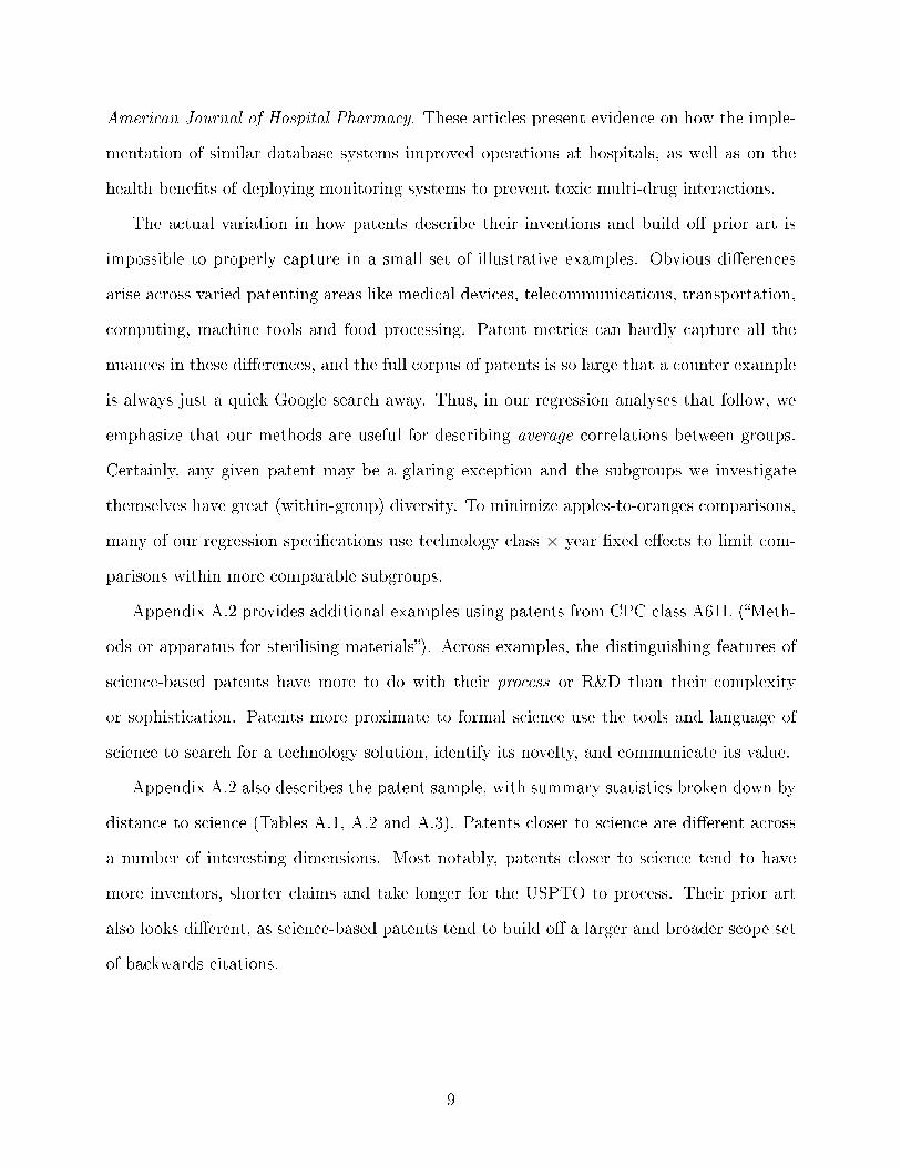
American Journal of Hospital Pharmacy. These articles present evidence on how the imple-

mentation of similar database systems improved operations at hospitals, as well as on the

health bene�ts of deploying monitoring systems to prevent toxic multi-drug interactions.

The actual variation in how patents describe their inventions and build o� prior art is

impossible to properly capture in a small set of illustrative examples. Obvious di�erences

arise across varied patenting areas like medical devices, telecommunications, transportation,

computing, machine tools and food processing. Patent metrics can hardly capture all the

nuances in these di�erences, and the full corpus of patents is so large that a counter example

is always just a quick Google search away. Thus, in our regression analyses that follow, we

emphasize that our methods are useful for describing average correlations between groups.

Certainly, any given patent may be a glaring exception and the subgroups we investigate

themselves have great (within-group) diversity. To minimize apples-to-oranges comparisons,

many of our regression speci�cations use technology class × year �xed e�ects to limit com-

parisons within more comparable subgroups.

Appendix A.2 provides additional examples using patents from CPC class A61L (�Meth-

ods or apparatus for sterilising materials�). Across examples, the distinguishing features of

science-based patents have more to do with their process or R&D than their complexity

or sophistication. Patents more proximate to formal science use the tools and language of

science to search for a technology solution, identify its novelty, and communicate its value.

Appendix A.2 also describes the patent sample, with summary statistics broken down by

distance to science (Tables A.1, A.2 and A.3). Patents closer to science are di�erent across

a number of interesting dimensions. Most notably, patents closer to science tend to have

more inventors, shorter claims and take longer for the USPTO to process. Their prior art

also looks di�erent, as science-based patents tend to build o� a larger and broader scope set

of backwards citations.

9

4 Results

In the following, we �rst map the relation between private sector value and distance to

science. We show that patents closer to science have a higher value than patents further

away from science. In a second step we show that patents that are more novel are also more

valuable. Lastly, we show that patents closer to science are also more novel, highlighting a

potential reason why science-based patents are more valuable.

4.1 The private value of patents by their distance to science

Our �rst fact documents the relationship between patent values and distance to science.

We show that more science-intensive patents are on average more valuable but also riskier;

i.e., they are more likely to be in the tails of the value distribution.

[Insert Figure 1 Here]

We start by presenting how relative dollar values of patents di�er by distance from science.

To estimate relative (%) di�erences in KPSS values across distance to science groups, we run

ordinary least squares (OLS) regressions with (D=4) as the baseline (omitted) distance to

science group.8 We then convert the regression coe�cients to percentage di�erences relative

to (D=4) average values. As shown in Panel (a) of Figure 1, a science-based patent that

directly cites an academic article (D=1) has an average value that is 82% greater than a

patent four degrees removed from science (D=4). This value decreases as the distance to

science increases. Patents with a distance of two or three have average values 44% and 14%

higher than those in (D=4), respectively. When patents have a distance from science larger

than four (D=5, D>5 or �unconnected�), their average values are between 6% and 16% less

valuable than those with distance of four. Column (1) of Table 1 presents the same results

in regression form.

8Distance to science of four as the baseline is an arbitrary choice, but one informed by the data, since therelative value premium begins to �atten after (D=4). Intuitively, the connection to scienti�c publicationsis quite tenuous at (D=4), and using this baseline group also ensures that our estimates are somewhatconservative vs. using higher degrees as the baseline.

10

[Insert Table 1 Here]

Our preferred speci�cations report patent value di�erences in relative (%) terms, but

to get a sense of the order of magnitude, we present the same results in levels ($USD) in

Appendix B.1 (Table A.5).9 We interpret the dollar magnitudes with caution, adjusting

the KPSS values downwards using the most conservative estimate of ex-ante probability of

patent grant. Doing so de�ates the values by 12%.10 Thus, we �nd that a science-based

patents that directly cites an academic article (D=1) have an average value of $15.82 million

dollars, which is $8.27 million more than the average value of patents with (D=4) and $8.69

million more than those unconnected to science.11 The average patent values decline to

$12.49, $9.90, and $8.69 million for distances of two, three and four, respectively.

The higher average value of science-based patents re�ects an upward shift in the value

distribution of patents with higher science intensity. Panel (b) of Figure 1 plots the share

of science-intensive patents (D=1, D=2 and D=3) and the share of less-science intensive

patents (D=4, D=5, D>5 and unconnected) over the percentiles of the value distribution of

all patents. If the value distribution of more science-intensive patents were the same as the

value distribution of less science-intensive patents, the share of patents at each percentile

should be 1%. Figure 1, Panel (b) shows that there are fewer science-intensive patents at

the lower end of the value distribution while there are more at the upper end. The pattern

for less-science-intensive patents is (mechanically) reversed. They are overrepresented at

9To arrive at dollar values for individual patents, (Kogan et al., 2017) makes a number of assumptionsabout the distribution of �rm returns and the (ex-ante) probability of patent grants. While the (Koganet al., 2017) results appear fairly robust to alternative distributional assumptions (see Footnote 11 in (Koganet al., 2017)), we focus on percentage di�erences as our primary results since our interest is in the relativevalue di�erences patents of di�erent characteristics. Doing so allows us to apply the consistent quantitativevaluation method of (Kogan et al., 2017), without relying too heavily on any assumptions that move themagnitude in any direction.

10Carley et al. (2015) �nd acceptance rates vary between 50% and 60% in the 1991�2001 period. We usethe low end of that range (50%) instead of the average (56%), which is used in Kogan et al. (2017). Thisadjustment de�ates all the patent dollar values by 12%. Conceptually, this adjustment provides a moreconservative set of estimates by increasing the amount of market information �surprise� associated with thepatent grant. That increased surprise could be a result of more conservative expectations about likelihoodof patent issuance, or imperfect information regarding the existence of pending patent applications. TableA.4 in Appendix B.2 shows how di�erent assumptions on patent grant probabilities a�ect patent valuations.

117.13/8.69 = 0.82%, the percent di�erence in value of a science-based patent relative to (D=4) patentmentioned above.

11

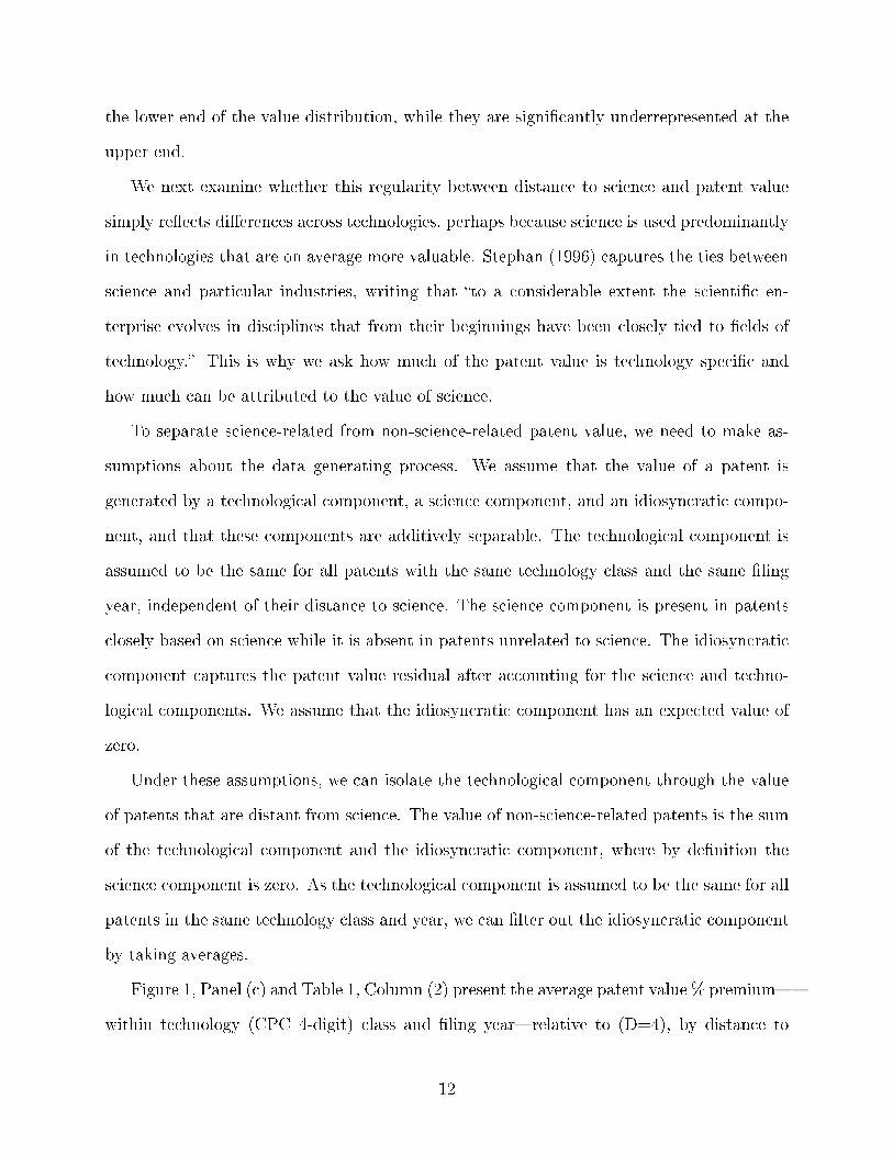
the lower end of the value distribution, while they are signi�cantly underrepresented at the

upper end.

We next examine whether this regularity between distance to science and patent value

simply re�ects di�erences across technologies, perhaps because science is used predominantly

in technologies that are on average more valuable. Stephan (1996) captures the ties between

science and particular industries, writing that �to a considerable extent the scienti�c en-

terprise evolves in disciplines that from their beginnings have been closely tied to �elds of

technology.� This is why we ask how much of the patent value is technology speci�c and

how much can be attributed to the value of science.

To separate science-related from non-science-related patent value, we need to make as-

sumptions about the data generating process. We assume that the value of a patent is

generated by a technological component, a science component, and an idiosyncratic compo-

nent, and that these components are additively separable. The technological component is

assumed to be the same for all patents with the same technology class and the same �ling

year, independent of their distance to science. The science component is present in patents

closely based on science while it is absent in patents unrelated to science. The idiosyncratic

component captures the patent value residual after accounting for the science and techno-

logical components. We assume that the idiosyncratic component has an expected value of

zero.

Under these assumptions, we can isolate the technological component through the value

of patents that are distant from science. The value of non-science-related patents is the sum

of the technological component and the idiosyncratic component, where by de�nition the

science component is zero. As the technological component is assumed to be the same for all

patents in the same technology class and year, we can �lter out the idiosyncratic component

by taking averages.

Figure 1, Panel (c) and Table 1, Column (2) present the average patent value % premium�

within technology (CPC 4-digit) class and �ling year�relative to (D=4), by distance to

12

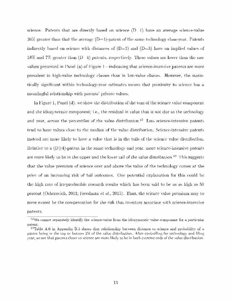
science. Patents that are directly based on science (D=1) have an average science-value

26% greater than that the average (D=4)-patent of the same technology class-year. Patents

indirectly based on science with distances of (D=2) and (D=3) have an implied values of

18% and 7% greater than (D=4) patents, respectively. These values are lower than the raw

values presented in Panel (a) of Figure 1�indicating that science-intensive patents are more

prevalent in high-value technology classes than in low-value classes. However, the statis-

tically signi�cant within technology-year estimates means that proximity to science has a

meaningful relationship with patents' private values.

In Figure 1, Panel (d), we show the distribution of the sum of the science value component

and the idiosyncratic component; i.e., the residual in value that is not due to the technology

and year, across the percentiles of the value distribution.12 Less science-intensive patents

tend to have values close to the median of the value distribution. Science-intensive patents

instead are more likely to have a value that is in the tails of the science value distribution.

Relative to a (D≥4)-patent in the same technology and year, more science-intensive patents

are more likely to be in the upper and the lower tail of the value distribution.13 This suggests

that the value premium of science over and above the value of the technology comes at the

price of an increasing risk of tail outcomes. One potential explanation for this could be

the high rate of irreproducible research results which has been said to be as as high as 50

percent (Osherovich, 2011; Freedman et al., 2015). Thus, the science value premium may to

some extent be the compensation for the risk that investors associate with science-intensive

patents.

12We cannot separately identify the science-value from the idiosyncratic value component for a particularpatent.

13Table A.6 in Appendix B.5 shows that relationship between distance to science and probability of apatent being in the top or bottom 5% of the value distribution. After controlling for technology and �lingyear, we see that patents closer to science are more likely to be in both extreme ends of the value distribution.

13

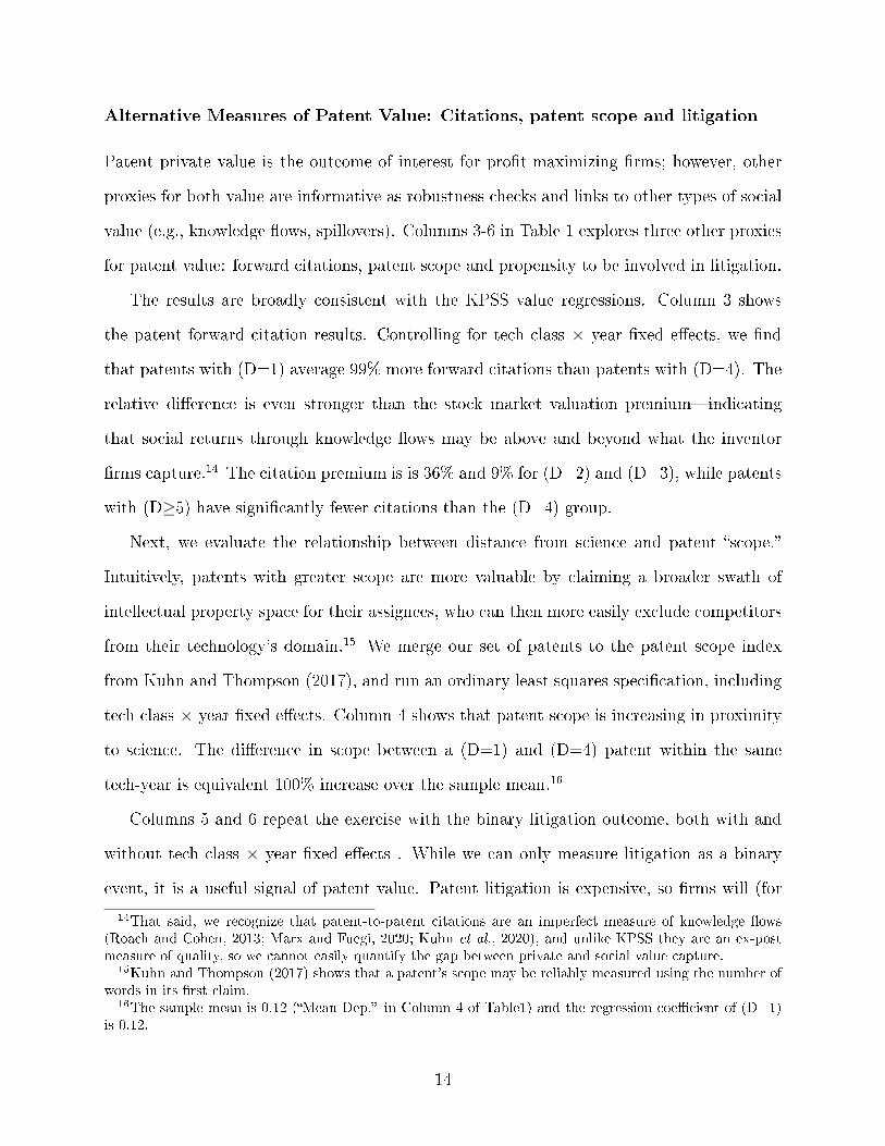
Alternative Measures of Patent Value: Citations, patent scope and litigation

Patent private value is the outcome of interest for pro�t-maximizing �rms; however, other

proxies for both value are informative as robustness checks and links to other types of social

value (e.g., knowledge �ows, spillovers). Columns 3-6 in Table 1 explores three other proxies

for patent value: forward citations, patent scope and propensity to be involved in litigation.

The results are broadly consistent with the KPSS value regressions. Column 3 shows

the patent forward citation results. Controlling for tech class × year �xed e�ects, we �nd

that patents with (D=1) average 99% more forward citations than patents with (D=4). The

relative di�erence is even stronger than the stock market valuation premium�indicating

that social returns through knowledge �ows may be above and beyond what the inventor

�rms capture.14 The citation premium is is 36% and 9% for (D=2) and (D=3), while patents

with (D≥5) have signi�cantly fewer citations than the (D=4) group.

Next, we evaluate the relationship between distance from science and patent �scope.�

Intuitively, patents with greater scope are more valuable by claiming a broader swath of

intellectual property space for their assignees, who can then more easily exclude competitors

from their technology's domain.15 We merge our set of patents to the patent scope index

from Kuhn and Thompson (2017), and run an ordinary least squares speci�cation, including

tech class × year �xed e�ects. Column 4 shows that patent scope is increasing in proximity

to science. The di�erence in scope between a (D=1) and (D=4) patent within the same

tech-year is equivalent 100% increase over the sample mean.16

Columns 5 and 6 repeat the exercise with the binary litigation outcome, both with and

without tech class × year �xed e�ects . While we can only measure litigation as a binary

event, it is a useful signal of patent value. Patent litigation is expensive, so �rms will (for

14That said, we recognize that patent-to-patent citations are an imperfect measure of knowledge �ows(Roach and Cohen, 2013; Marx and Fuegi, 2020; Kuhn et al., 2020), and unlike KPSS they are an ex-postmeasure of quality, so we cannot easily quantify the gap between private and social value capture.

15Kuhn and Thompson (2017) shows that a patent's scope may be reliably measured using the number ofwords in its �rst claim.

16The sample mean is 0.12 (�Mean Dep.� in Column 4 of Table1) and the regression coe�cient of (D=1)is 0.12.

14

the most part) only �ght in court for patents that are believed to be valuable.17 18 With and

without class by year �xed e�ects, we �nd that the likelihood of litigation is increasing in

proximity to science. Column 5 indicates that patents with (D=1) have a more than double

increased likelihood of litigation relative to D=4 patents (10.4 vs. 4.4 per 1,000 patents).

Column 6 shows that even within tech class and vintage, patents that build more directly

on science are more likely to end up in court. Taken together with the KPSS, citation and

scope results, this �nding shows patents that build more directly on science are not only

valued higher, but �rms judge them more worthy of expensive courtroom battles in the

years post-grant.

Additional Results and Robustness

Appendix B and C present a number of additional results and robustness checks. Appendix

B.3 shows results by broad (1-digit) CPC classes. Appendix B.4 shows how the distance

to science measure e�ectively captures which patents are drawing more directly on the lan-

guage and ideas of their associated scienti�c journal articles. Appendix B.5 describes the

regressions examining the tails of the value distribution. We show that the main distance

to science results hold up across di�erent percentiles of the value distribution in Appendix

B.6. Appendix B.7 shows how KPSS values vary by both distance to science and novelty.

Appendix C show robustness to alternative method choices�including di�erent distance to

science measures (Appendix C.1), using di�erent normalizations and assignee �xed e�ects

(Appendix C.2), and the intensity of citations within the (D=1) group (Appendix C.3).

17The American Intellectual Property Lawyer's Association (AIPLA) estimated litigation costs of$250,000 � $950,000 for cases with less than $1 million at risk, and between $2.4 million and $4 mil-lion for cases with more at stake (https://apnews.com/press-release/news-direct-corporation/a5dd5a7d415e7bae6878c87656e90112)

18The dependent variable comes from merging our data to the USPTO's Patent Number and Case Code Filedataset, a comprehensive link between patent litigation cases in U.S. district courts and patents between 2003and 2016. 94% of the court cases are coded as patent infringement suits, with the remaining cases involvingdisputes around ownership/inventorship, patent validity, royalties, false markings, and other proceduralissues involving patents.

15

4.2 Patent novelty and patent value

Next, we study whether the value of a patent is related to the novelty of its content. If the

goal of science is to advance knowledge by making new discoveries, then inventions relying

directly on science have the potential to introduce more novel ideas. For these analyses, we

construct a new measure of patent novelty. Using this measure, we establish the second

fact of the paper: that patent novelty predicts patent values.

Measuring patent novelty

In the history of technology and innovation, inventions are often conceptualized as the out-

come of successfully combining ideas, either by combining new ideas or by combining existing

ones in a novel way. In A History of Mechanical Inventions, Abbott Payson Usher writes:

�Invention �nds its distinctive feature in the constructive assimilation of preexisting elements

into new syntheses, new patterns, or new con�gurations of behavior� (Weitzman, 1998). Fol-

lowing this concept of invention as a novel combination of ideas or resources, we develop a

new measure for patent novelty that is based on the content of the patent. More speci�cally,

we measure how novel the combinations of words are that are used in a patent. For example,

the word �mouse� combined with the word �trap� was used in patents since at least 1870. In

contrast, the word �mouse� was combined with the word �display� for the �rst time in 1981

in the pioneering patents of Xerox.

Our measure of patent novelty is constructed as follows. In a �rst step, we count how often

a particular pairwise combination of di�erent words was used in the abstracts of previous

patents up to the �ling year. The sets of words for every patent are taken from the dataset of

Arts et al. (Arts et al., 2018). We then divide this count with the total number of pairwise

word combinations up to the �ling year of the patent. We denote this ratio as the probability

of a word combination. In a second step, we take the average over the respective probabilities

of all pairwise word combinations within a patent to determine the average probability per

patent. The smaller the average probability of pairwise word combinations, the more novel

16

are the pairwise word combinations used in the particular patent. We call patents with

a smaller average probability more novel. Appendix C.4 provides similar analyses using

alternative de�nitions of patent novelty such as new words and word age (Figure A.8), as

well as chemical novelty (Table A.7). The correlations between these alternative measures

and KPSS patent value and distance to science are quite similar to our main measure of

novelty.

Novelty and patent value

Figure 2 shows that the novelty of a patent � measured by the average probability of word

combinations � predicts the patent value and the likelihood that the value of a patent is in

the tails of the distribution. Panel (a) shows that there is a positive relationship between

novelty and patent value. The pattern suggests increasing returns to novelty, as the marginal

gains from novelty increase as word combinations become more rare. Panel (b) indicates that

a higher patent novelty is associated with an upward shift in the patent value distribution.

We split all patents into those that have a below average probability of word combinations

(i.e., higher novelty) and those that have an above average probability. Panel (b) shows that

more novel patents (i.e., patents with a low probability of word combinations) are less likely

to be at the lower end of the value distribution and more likely to be at the upper end. The

picture is reversed for patents that are less novel.


In Panel (c), we plot the relationship between patent novelty and patent value relative

to (D=4)-patent values of the same technology and the same year. We also residualize the

novelty measure (x-axis), such that x-axis values below (above) zero represent combinations

of words that are less (more) common than the average word combinations within technology-

year. Again, there is a clear positive relationship between novelty and science value.19 In

19The regression version of this analysis is reported in Columns 1 and 2 of Table 2 (without and withtechnology × year �xed e�ects). This speci�cation di�ers from the one presented in Figure 2, because here

17

Panel (d), we show the distribution of patent values for patents with below and above

average probability of word combinations relative to the probability of a (D=4)-patent in

the same technology and year. Highly novel patents are again more likely to be in both

tails of the value distribution while patents with a lower novelty are in the middle of the

value distribution, relative to its technology and year. Thus, as in the case of distance to

science, novelty is associated with a value premium over and above the technology-related

value component, but also with higher risk. Kline and Rosenberg (1986) captured the spirit

of this relationship in writing, �newness is not, by itself, an economic advantage.�

[Insert Table 2 Here]

4.3 Patent novelty and distance to science

As argued above, there are two complementary ways in which science can increase patent

novelty. First, science might provide new insights that can be combined with older ideas.

This view is akin to how Vannevar Bush described the relation between science and invention

in his in�uential 1945 report Science: The endless frontier :

Basic science (...) creates the fund from which the practical applications of knowl-

edge must be drawn. New products and new processes do not appear full-grown.

They are founded on new principles and new conceptions, which in turn are

painstakingly developed by research in the purest realms of science. Today, it

is truer than ever that basic research is the pacemaker of technological progress.

(Bush, 1945).

This description is thought to re�ect the realities in the large science-intensive corporate

laboratories of the post-war period (Smith and Hounshell, 1985; Godin, 2006).

we take the averages over all patents in a technology and year combination and not only over patents with adistance of D=4. The negatively and statistically signi�cant correlations in both speci�cations indicate thatthat patent value is decreasing in the likelihood of word combinations.

18

Second, science can guide the inventor to more fruitful combinations of known elements

(Rosenberg et al., 1990; Fleming and Sorenson, 2004). According to mathematician Henri

Poincare, �the true work of the inventor consists in choosing among (...) combinations so

as to eliminate the useless ones or rather to avoid the trouble of making them� (Weitzman,

1998).

Science can help tell which combinations not to pursue by providing an understanding of

why a combination might or might not work. For example, enormous amounts of energy and

ingenuity were wasted by alchemists on attempts to transform lead into gold before science

demonstrated that nothing short of an atomic reaction could achieve this end. Scienti�c

knowledge also guided the development of the Haber-Bosch method to synthesize ammonia.

During the �rst trial runs, Carl Bosch struggled with the problem that the hydrogen proved

to be corrosive for the high-pressure reactor chamber made of steel. Using basic chemistry,

he deduced that the problem was due to the carbon contained in the steel walls of the

chamber. His solution was to build a double wall reactor chamber with iron on the inside,

which contains no carbon, and steel on the outside (Je�reys, 2008).

In our �nal set of analyses, we explore the relationship between novel combinations of

ideas and proximity to science. The strikingly similar patterns displayed in Figures 1 and

2 suggests that the novelty of patents and their distance to science are related. Consistent

with this intuition, we establish as a third fact : patents that are more science-intensive

exhibit a higher patent novelty on average.

In Panels (a) and (b) of Figure 3, we show the novelty distributions for relatively more

science-intensive patents (D=1, D=2, D=3) and for relatively less science-intensive patents

(D=4, D=5, D>5, unconnected). As de�ned above, the lower the likelihood of a pairwise

word combination in a patent is, the more novel is the patent. Panel shows the novelty

distribution for the raw data. In Panel (b) of Figure 3, we adjust for di�erences in technology

and year. The novelty distribution for more science-intensive patents has its peak to the left

and at a higher density than the novelty distribution for less science-intensive patents, both

19

in the raw data and when controlling for technologies. This con�rms that patents closer

to science contain more novel word combinations; i.e., they are more novel (on average).

Columns 3 and 4 of Table 2 exhibit this relationship in regression form. In the averages

(Column 3) and within technology-year (Column 4), we see that novelty is decreasing with

distance to science�i.e., word combinations become, on average, as patents move further

away from connections to science.


However, we also observe that the relationship is non-linear and asymmetric. While

patents more proximate to science are less likely to be in the �less novel� half of the distribu-

tion (right tail), they are also less likely to be in the far left tail of the novelty distribution.

This asymmetry suggests that connection to science is associated with middle and above

average novelty, while the extreme novel patents are more likely to be distant from science.

Perhaps, those unconnected to science are less constrained in language (or imagination) than

inventions tethered by the norms and formalities of science. In Appendix C.4, we show that

these �ndings are robust to using the emergence of new words, the average age of words, of

patent chemical novelty as alternative novelty indicators.

Finally, we combine our measures of distance to science and novelty to assess whether

they separately contribute to patent value. The results are presented in Appendix B.7. We

interact distance to science with indicators for below and above median novelty, using the

same patent novelty measure as Figure 2 (Panels (c) and (d)). Speci�cally, patents are below

(above) median novelty if they have new word combinations that are below (above) median

for their CPC (4 digit) class and year. We then generate graphs equivalent to Figure 1

(Panels (a) and (c)) for the below median and above median novelty groups. The results

show very similar patterns for both groups. Both with and without adjusting for tech class

× year, we see that relative patent value is increasing in proximity to science. The same is

true regardless of whether we look at % di�erences or average patent dollar values (Panels

(c) and (d) of Appendix Figure A.4).

20

While the relationship between distance to science and relative patent value is quite sim-

ilar for both novelty groups, Appendix Figure A.4 shows that patent values are consistently

higher (shifted upward) for the high novelty sub-groups. Thus, novelty and science appear

to both contribute to private value. Since the two characteristics are at least partially co-

determined,20 we cannot quantify their relative in�uence on patent values. However, since

both novelty subgroups have patent values increasing in their proximity to science, novelty is

clearly not the sole mechanism behind our main results. Rather, we interpret these patterns

as evidence that using science as a tool to explore and express new ideas is a path associated

with both greater novelty and value capture.

5 Conclusion

Our study shows that building more directly on science is associated with more novel in-

ventions and capturing greater private value from those inventions. Thus, while scientists

since Isaac Newton have been known to see further �by standing on the shoulders of giants,�

our study suggests that many inventors in the private sector see further by standing on the

shoulders of science.

By their nature, our estimates provide an incomplete picture for the private value derived

from science. Beyond patented inventions, R&D organizations bene�t from applying the

tools and training born in the scienti�c community. These indirect bene�ts are possible

because �rms hire scientists and engage with the research frontier (Cohen and Levinthal,

1990; Henderson and Cockburn, 1994; Stern, 2004).

Along with the increased expected rewards from science, our results show that building

on science is a relatively risky approach to corporate innovation. We �nd that patents closer

to science and relatively novel patents are both more likely to end up in the tails of the

20In addition to the patterns found in Figure 3, Figure A.4 in Appendix B.7 demonstrates the strongcorrelation between novelty and proximity to science, as the two panels that adjust for technology × year�xed e�ects (Panels (b) and (d)) exhibit much bigger di�erences between the low vs. high novelty subgroupsthan what we see in the unadjusted raw di�erences (Panels (a) and (b)).

21

patent value distribution. This risk-reward trade o� helps explain why (risk-averse) �rms

often favor more certain technological exploitation and acquisitions over novel exploration.

Together, our results suggest science helps �rms push the technological frontier by build-

ing on more disparate ideas to introduce and combine more novel technologies�many of

which fall �at commercially, while others propel their �rm's growth. While its value is seem-

ingly available for science-driven �rms to capture, science's potential in corporate innovation

remains an important area for study. How best to access, engage with and build upon the

ever-expanding base of scienti�c knowledge and methods is an exciting challenge for both

R&D managers and scholars.

22

References

Ahmadpoor, M. and Jones, B. F. (2017). The dual frontier: Patented inventions and prior scienti�cadvance. Science, 357 (6351), 583�587.

Akcigit, U. and Kerr, W. R. (2018). Growth through heterogeneous innovations. Journal of PoliticalEconomy, 126 (4), 1374�1443.

Argote, L. and Greve, H. R. (2007). A behavioral theory of the �rm 40 years and counting: Introductionand impact. Organization Science, 18 (3), 337�349.

Arora, A., Belenzon, S. and Dionisi, B. (2021). First-mover Advantage and the Private Value of PublicScience. Tech. rep., National Bureau of Economic Research.

�, � and Patacconi, A. (2018). The decline of science in corporate r&d. Strategic Management Journal,39 (1), 3�32.

�, � and Sheer, L. (2020). Knowledge spillovers and corporate investment in scienti�c research. TheAmerican Economic Review, forthcoming.

�, Fosfuri, A. and Gambardella, A. (2004). Markets for Technology: The Economics of Innovationand Corporate Strategy. The MIT Press, MIT Press.

Arts, S., Cassiman, B. and Gomez, J. C. (2018). Text matching to measure patent similarity. StrategicManagement Journal, 39 (1), 62�84.

Azoulay, P., Furman, J. L., Krieger, J. L. andMurray, F. (2015). Retractions. Review of Economicsand Statistics, 97 (5), 1118�1136.

�, Graff Zivin, J. S., Li, D. and Sampat, B. N. (2019). Public R&D investments and private-sectorpatenting: evidence from NIH funding rules. Tech. Rep. 1.

�, � and Manso, G. (2011). Incentives and creativity: evidence from the academic life sciences. TheRAND Journal of Economics, 42 (3), 527�554.

Backman, T. W., Cao, Y. and Girke, T. (2011). Chemmine tools: an online service for analyzing andclustering small molecules. Nucleic acids research, 39 (suppl_2), W486�W491.

Begley, C. G. and Ellis, L. M. (2012). Raise standards for preclinical cancer research. Nature, 483 (7391),531�533.

� and Ioannidis, J. P. (2015). Reproducibility in science: improving the standard for basic and preclinicalresearch. Circulation research, 116 (1), 116�126.

Bhaskarabhatla, A. and Hegde, D. (2014). An organizational perspective on patenting and open inno-vation. Organization Science, 25 (6), 1744�1763.

Bikard, M. (2018). Made in academia: The e�ect of institutional origin on inventors' attention to science.Organization Science, 29 (5), 818�836.

� andMarx, M. (2020). Bridging academia and industry: How geographic hubs connect university scienceand corporate technology. Management Science, 66 (8), 3425�3443.

�, Vakili, K. and Teodoridis, F. (2019). When collaboration bridges institutions: The impact of uni-versity industry collaboration on academic productivity. Organization Science, 30 (2), 426�445.

Bloom, N., Jones, C. I., Van Reenen, J. and Webb, M. (2020). Are ideas getting harder to �nd?American Economic Review, 110 (4), 1104�44.

23

Bush, V. (1945). Science, the endless frontier: A report to the President. US Govt. print. o�.

Butler, D. (2008). Translational research: crossing the valley of death. Nature News, 453 (7197), 840�842.

Carley, M., Hedge, D. and Marco, A. (2015). What is the probability of receiving a us patent. Yale JL& Tech., 17, 203.

Chesbrough, H., Vanhaverbeke, W. and West, J. (2006). Open Innovation: Researching a NewParadigm. OUP Oxford.

Cockburn, I. M., Henderson, R. M. and Stern, S. (2000). Untangling the origins of competitiveadvantage. Strategic Management Journal, 21 (10/11), 1123�1145.

Cohen, W. M. and Levinthal, D. A. (1990). Absorptive capacity: A new perspective on learning andinnovation. Administrative Science Quarterly, 35 (1), 128�152.

Cyert, R. M., March, J. G. et al. (1963). A behavioral theory of the �rm, vol. 2. Englewood Cli�s, NJ.

Eggers, J. P. (2012). Falling �at: Failed technologies and investment under uncertainty. AdministrativeScience Quarterly, 57 (1), 47�80.

Ewens, M., Nanda, R. and Rhodes-Kropf, M. (2018). Cost of experimentation and the evolution ofventure capital. Journal of Financial Economics, 128 (3), 422 � 442.

Fleming, L. and Sorenson, O. (2004). Science as a map in technological search. Strategic ManagementJournal, 25 (8-9), 909�928.

Freedman, L. P., Cockburn, I. M. and Simcoe, T. S. (2015). The economics of reproducibility inpreclinical research. PLoS biology, 13 (6), e1002165.

Gans, J. S. and Stern, S. (2003). The product market and the market for ideas commercialization strate-gies for technology entrepreneurs. Research Policy, 32 (2), 333 � 350, special Issue on Technology En-trepreneurship and Contact Information for corresponding authors.

Godin, B. (2006). The linear model of innovation: The historical construction of an analytical framework.Science, Technology, & Human Values, 31 (6), 639�667.

Goozner, M. (2005). The $800 million pill: The truth behind the cost of new drugs. Univ of Californiapress.

Hall, B. H., Jaffe, A. B. and Trajtenberg, M. (2001). The nber patent citation data �le: Lessons,insights and methodological tools. NBER Working Paper No. 8498.

� and Lerner, J. (2010). The �nancing of r&d and innovation. In B. H. Hall and N. Rosenberg (eds.),Handbook of The Economics of Innovation, Vol. 1, Handbook of the Economics of Innovation, vol. 1,North-Holland, pp. 609�639.

Harris, G. (2011). Federal research center will help develop medicines. New York Times, (January 22).

Henderson, R. and Cockburn, I. (1994). Measuring competence? exploring �rm e�ects in pharmaceuticalresearch. Strategic Management Journal, 15 (S1), 63�84.

Iaria, A., Schwarz, C. andWaldinger, F. (2018). Frontier knowledge and scienti�c production: evidencefrom the collapse of international science. The Quarterly Journal of Economics, 133 (2), 927�991.

Jeffreys, D. (2008). Hell's cartel: IG Farben and the making of Hitler's war machine. Macmillan.

24

Jones, B. F. (2009). The burden of knowledge and the death of the renaissance man: Is innovation gettingharder? The Review of Economic Studies, 76 (1), 283�317.

Kelly, B., Papanikolaou, D., Seru, A. and Taddy, M. (2018). Measuring technological innovation overthe long run. Tech. rep., Working Paper.

Kline, S. J. and Rosenberg, N. (1986). An overview of innovation. the positive sum strategy: Harnessingtechnology for economic growth. The National Academy of Science, USA.

Kogan, L., Papanikolaou, D., Seru, A. and Stoffman, N. (2017). Technological innovation, resourceallocation, and growth. The Quarterly Journal of Economics, 132 (2), 665�712.

Krieger, J., Li, D. and Papanikolaou, D. (2021). Missing Novelty in Drug Development*. The Reviewof Financial Studies, hhab024.

Kuhn, J., Younge, K. and Marco, A. (2020). Patent citations reexamined. The RAND Journal ofEconomics, 51 (1), 109�132.

Kuhn, J. M. and Thompson, N. (2017). How to measure and draw causal inferences with patent scope.

Magerman, T., Van Looy, B. and Debackere, K. (2015). Does involvement in patenting jeopardizeone's academic footprint? an analysis of patent-paper pairs in biotechnology. Research Policy, 44 (9),1702�1713.

Mansfield, E. (1991). Academic research and industrial innovation. Research policy, 20 (1), 1�12.

� (1995). Academic research underlying industrial innovations: sources, characteristics, and �nancing.Review of Economics and Statistics, 77 (1), 55�65.

� (1998). Academic research and industrial innovation: An update of empirical �ndings. Research policy,26 (7-8), 773�776.

Manso, G. (2011). Motivating innovation. The Journal of Finance, 66 (5), 1823�1860.

March, J. G. (1991). Exploration and exploitation in organizational learning. Organization Science, 2 (1),71�87.

Marco, A. C., Tesfayesus, A. and Toole, A. A. (2017). Patent litigation data from us district courtelectronic records (1963-2015).

Marx, M. and Fuegi, A. (2020). Reliance on science: Worldwide front-page patent citations to scienti�carticles. Strategic Management Journal, 41 (9), 1572�1594.

Mowery, D. C. (2009). Plus ca change, industrial rd in the third industrial revolution. Industrial andCorporate Change, 18 (1), 1�50.

Murray, F. (2002). Innovation as co-evolution of scienti�c and technological networks: exploring tissueengineering. Research policy, 31 (8-9), 1389�1403.

� and Stern, S. (2007). Do formal intellectual property rights hinder the free �ow of scienti�c knowledge?an empirical test of the anti-commons hypothesis. Journal of Economic Behavior and Organization, 63 (4),648�687.

Osherovich, L. (2011). Hedging against academic risk. Science-Business eXchange, 4 (15), 416�416.

Partha, D. and David, P. A. (1994). Toward a new economics of science. Research policy, 23 (5), 487�521.

25

Poege, F., Harhoff, D., Gaessler, F. and Baruffaldi, S. (2019). Science quality and the value ofinventions. arXiv preprint arXiv:1903.05020.

Roach, M. and Cohen, W. M. (2013). Lens or prism? patent citations as a measure of knowledge �owsfrom public research. Management Science, 59 (2), 504�525.

Rosenberg, N. et al. (1990). Why do �rms do basic research (with their own money)? Research Policy,19 (2), 165�174.

Schmoch, U. (2008). Concept of a technology classi�cation for country comparisons. Final report to theworld intellectual property organisation (wipo), WIPO.

Sinha, A., Shen, Z., Song, Y., Ma, H., Eide, D., Hsu, B.-j. P. and Wang, K. (2015). An overview ofmicrosoft academic service (mas) and applications. In Proceedings of the 24th international conference onworld wide web, ACM, pp. 243�246.

Smith, J. K. and Hounshell, D. A. (1985). Wallace h. carothers and fundamental research at du pont.Science, 229 (4712), 436�442.

Sorenson, O. and Fleming, L. (2004). Science and the di�usion of knowledge. Research policy, 33 (10),1615�1634.

Stephan, P. E. (1996). The economics of science. Journal of Economic literature, 34 (3), 1199�1235.

� (2012). How economics shapes science, vol. 1. Harvard University Press Cambridge, MA.

Stern, S. (2004). Do scientists pay to be scientists? Management Science, 50 (6), 835�853.

Stokes, D. E. (2011). Pasteur's quadrant: Basic science and technological innovation. Brookings InstitutionPress.

Tang, J., Zhang, J., Yao, L., Li, J., Zhang, L. and Su, Z. (2008). Arnetminer: extraction and min-ing of academic social networks. In Proceedings of the 14th ACM SIGKDD international conference onKnowledge discovery and data mining, ACM, pp. 990�998.

von Hippel, E. (1988). The Sources of Innovation. Oxford University Press.

Weitzman, M. L. (1998). Recombinant growth. Quarterly Journal of Economics, pp. 331�360.

Wuchty, S., Jones, B. F. and Uzzi, B. (2007). The increasing dominance of teams in production ofknowledge. Science, 316 (5827), 1036�1039.

26

Tables & Figures

-20%

0%

20%

40%

60%

80%

100%

1 2 3 4 5 >5 unconnected

Distance to science

Mean90% confidence bounds

% more valuable than patents with distance to science of 4

(a) Averages

.4

.6

.8

1

1.2%

0 20 40 60 80 100Percentiles of the patent value distribution

D=1, D=2 and D=3 D=4, D>4 and unconn.

Share of patents

(b) Distribution

-10%

0%

10%

20%

30%


Distance to science


% more valuable than patents with distance to science of 4in same technology class and with the same filing year

(c) Averages accounting for technology and year

.4

.6

.8

1

1.2

1.4%


D=1, D=2 and D=3 D=4, D>4 and unconn.

Share of patents

(d) Distribution accounting for technology and year

Figure 1: Distance to science, patent value and risk.

Panel (a) shows the average patent value for all distances to science relative to patents with a distance offour (D=4). The values of U.S. patents are from Kogan et al. (2017). The distance to science of U.S. patentsis calculated using data from Marx and Fuegi (2020) and the method of Ahmadpoor and Jones (2017).The distance to science is de�ned by citation links. The values correspond to the coe�cients in Table 1,Column 1. Panel (b) shows the distribution of patent values across the percentiles of the value distributionof all patents for more science-intensive patents (D=1, D=2 or D=3; solid red line) and less science-intensivepatents (D>3 or unconnected; dashed blue line). The horizontal line at 1% shows the distribution of allpatents across the percentiles of the value distribution. In Panel (c), we residualize the patent value by theaverage value of a patent with the same (four-digit) CPC technology class and �ling year and a distance offour, then display relative (%) values indexed to D=4. The values correspond to the coe�cients in Table 1,Column 2. In Panel (d), we show the distribution of the patent values normalized by technology and year.

27

5

10

15

20

25

0 .1 .2 .3Likelihood of word combinations in patent x 10^6

Average value in millions $USD

(a) Raw data

.4

.6

.8

1

1.2

1.4%


Newer word combinations than averageMore common word combinations than average

Share of patents

(b) Distribution

0

1

2

3

-.1 -.05 0 .05 .1 .15Likelihood of word combinations in patent x 10^6

Average value in millions $USD rel. tech x year

(c) Accounting for technology and year

.8

.85

.9

.95

1

1.05

1.1%

0 20 40 60 80 100Percentiles of the patent value distribution rel. tech x year

Newer word combinations than averageMore common word combinations than average

Share of patents

(d) Distribution accounting for technology and year

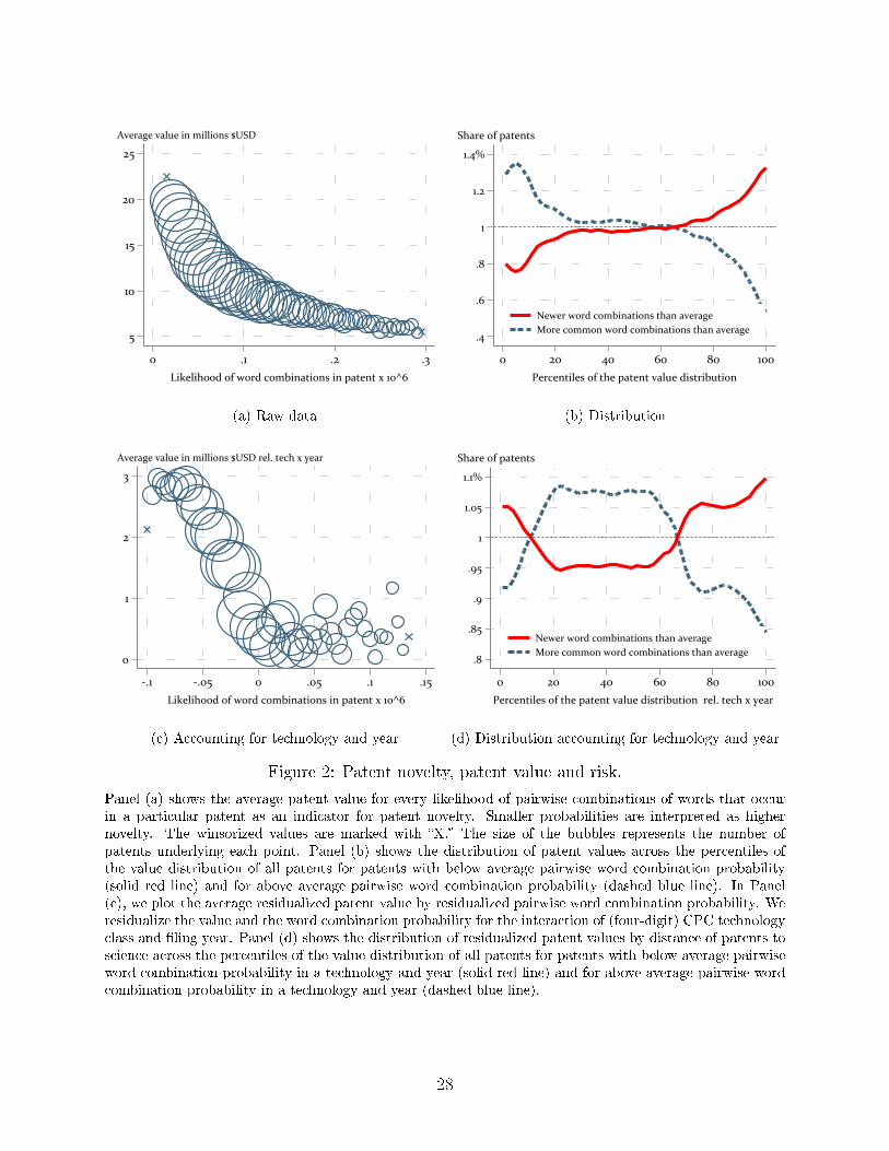
Figure 2: Patent novelty, patent value and risk.

Panel (a) shows the average patent value for every likelihood of pairwise combinations of words that occurin a particular patent as an indicator for patent novelty. Smaller probabilities are interpreted as highernovelty. The winsorized values are marked with �X.� The size of the bubbles represents the number ofpatents underlying each point. Panel (b) shows the distribution of patent values across the percentiles ofthe value distribution of all patents for patents with below average pairwise word combination probability(solid red line) and for above average pairwise word combination probability (dashed blue line). In Panel(c), we plot the average residualized patent value by residualized pairwise word combination probability. Weresidualize the value and the word combination probability for the interaction of (four-digit) CPC technologyclass and �ling year. Panel (d) shows the distribution of residualized patent values by distance of patents toscience across the percentiles of the value distribution of all patents for patents with below average pairwiseword combination probability in a technology and year (solid red line) and for above average pairwise wordcombination probability in a technology and year (dashed blue line).

28

0

2

4

6

8

0 .1 .2 .3 .4Likelihood of word combinations in patent x 10^6

D=1, D=2 and D=3D=4, D=5, D>5 and unconn.

Density

(a) Novelty distribution by science intensity

0

2

4

6

8

10

-.1 0 .1 .2 .3Likelihood of word combinations in patent rel. tech x year x 10^6

D=1, D=2 and D=3D=4, D=5, D>5 and unconn.

Density

(b) Accounting for technology and year

Figure 3: Patent novelty and distance to science.

Panel (a) shows the kernel density plot of the average likelihood of pairwise combinations of words thatoccur in a particular patent for more science-intensive patents (D=1, D=2 or D=3; red line) and for lessscience-intensive patents (D>3 or unconnected; dashed blue line). Smaller probabilities are interpreted as ahigher novelty. In Panel (b), we residualize the patent value and the likelihood of word combinations by theaverage value of a patent with the same technology class and �ling year and a distance of four.

29

(1) (2) (3) (4) (5) (6)

Patent Value

Outcome: Dollar Dollar Citations Patent Scope Prob(Litigation) x 1000

Distance 1 0.82∗∗∗ 0.26∗∗∗ 0.99∗∗∗ 0.12∗∗∗ 10.36∗∗∗ 4.40∗∗∗

(0.17) (0.04) (0.09) (0.03) (1.44) (0.62)Distance 2 0.44∗∗∗ 0.18∗∗∗ 0.36∗∗∗ 0.10∗∗∗ 6.77∗∗∗ 1.50∗∗∗

(0.11) (0.03) (0.04) (0.02) (0.60) (0.42)Distance 3 0.14∗∗∗ 0.07∗∗∗ 0.09∗∗∗ 0.07∗∗∗ 4.93∗∗∗ 0.16

(0.05) (0.02) (0.02) (0.01) (0.38) (0.34)Distance 4 4.39∗∗∗

(0.41)Distance 5 -0.06∗∗ -0.01 -0.06∗∗∗ -0.03∗ 3.88∗∗∗ -0.52

(0.03) (0.01) (0.01) (0.02) (0.40) (0.43)Distance >5 -0.16∗∗∗ -0.03∗ -0.14∗∗∗ -0.05∗∗ 3.43∗∗∗ -0.73∗

(0.04) (0.02) (0.02) (0.02) (0.30) (0.40)Unconnected -0.13∗ -0.01 -0.13∗∗∗ -0.04 2.49∗∗∗ -0.57

(0.07) (0.02) (0.03) (0.08) (0.26) (0.41)Tech x Year FE No Yes Yes Yes No YesMean Dep. 11.56 11.56 29.88 0.12 6.40 6.40Obs. 1135757 1135757 1135757 231474 1135757 1135757

Table 1: Patent Value MeasuresTable 1 reports regression results on how various patent value outcomes with the independent variableof distance to science. The calculation of distance-to-science is based on Ahmadpoor and Jones (2017).Unconnected patents are patents for which we could not �nd a citation link to any scienti�c article. Columns1�3 are generated by ordinary least squares (OLS) speci�cations, and we report the coe�cients in terms oftheir percentage increases relative to D=4. For example, the coe�cient for the �rst value in Column 1may be interpreted as an 82% increase relative to (D=4). In Column 1, the outcome is (adjusted) patentvalues from Kogan et al. (2017). In Column 2, we control for (four-digit) CPC technology class × �ling year�xed e�ects such that coe�cients represent relative di�erences within tech-year. In Column 3, the outcomevariable is the count of citing families. In Column 4, we use the within art unit patent scope index providedby Kuhn and Thompson (2017) as the outcome variable in an OLS regression. Columns 5 and 6 are bothOLS speci�cations where the outcome variable is an indicator variable for whether or not the focal patentwas ever involved in litigation (multiplied by 1000). The litigation outcome variable is based on the datafrom Marco et al. (2017). For all models, the standard errors are clustered on the CPC technology classlevel. *, ** and *** indicate that the coe�cient is signi�cantly di�erent from zero on the 10%, 5%, and 1%level.

30

(1) (2) (3) (4)

Patent value Patent novelty

Outcome: Dollar Dollar Probability of Probability ofword combination word combination

Distance 1 7.91∗∗∗ -1.69∗∗∗

(0.36) (0.18)Distance 2 9.37∗∗∗ -0.76∗∗∗

(0.28) (0.11)Distance 3 10.45∗∗∗ -0.23∗∗∗

(0.17) (0.07)Distance 4 11.90∗∗∗

(0.16)Distance 5 13.95∗∗∗ 0.30∗∗∗

(0.18) (0.07)Distance >5 16.58∗∗∗ 0.79∗∗∗

(0.20) (0.13)Unconnected 16.25∗∗∗ 0.39∗∗∗

(0.50) (0.11)Probability -43.39∗∗∗ -10.20∗∗∗

of word combinations (3.84) (1.47)Tech x Year FE No Yes No YesMean Dep. 11.56 11.56 10.45 10.45Obs. 1135669 1135669 1135669 1135669

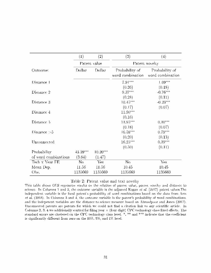
Table 2: Patent value and text noveltyThis table shows OLS regression results on the relation of patent value, patent novelty and distance toscience. In Columns 1 and 2, the outcome variable is the adjusted Kogan et al. (2017) patent values.Theindependent variable is the focal patent's probability of word combinations based on the data from Artset al. (2018). In Columns 3 and 4, the outcome variable is the patent's probability of word combinations,and the indepenent variables are the distance-to-science measure based on Ahmadpoor and Jones (2017).Unconnected patents are patents for which we could not �nd a citation link to any scienti�c article. InColumns 2, 3, 4 we additionally control for �ling year × (four-digit) CPC technology class �xed e�ects. Thestandard errors are clustered on the CPC technology class level. *, ** and *** indicate that the coe�cientis signi�cantly di�erent from zero on the 10%, 5%, and 1% level.

31

Appendices

A Data 2

A.1 Data Sources . . . . . . . . . . . . . . . . . . . . . . . . . . . . . . . . . . . 2

A.2 Patent Characteristics and Distance to Science . . . . . . . . . . . . . . . . . 6

B Additional Regressions and Robustness Results 11

B.1 Patent Value Outcomes (in Levels), by Distance to Science and Text Similarity 11

B.2 Di�erent assumptions for KPSS value estimates . . . . . . . . . . . . . . . . 12

B.3 Split by technology . . . . . . . . . . . . . . . . . . . . . . . . . . . . . . . . 14

B.4 Comparing Patent and Scienti�c Article Text . . . . . . . . . . . . . . . . . 16

B.5 Patent Tail Outcomes . . . . . . . . . . . . . . . . . . . . . . . . . . . . . . . 16

B.6 E�ects over the entire value distribution . . . . . . . . . . . . . . . . . . . . 18

B.7 Patent value by distance to science and novelty . . . . . . . . . . . . . . . . 19

C Alternative data and method choices 23

C.1 Using Ahmadpoor and Jones distance values . . . . . . . . . . . . . . . . . 23

C.2 Di�erent normalizations and assignee-�xed e�ects . . . . . . . . . . . . . . . 24

C.3 Number of citations to science and value . . . . . . . . . . . . . . . . . . . . 27

C.4 Alternative measures for novelty . . . . . . . . . . . . . . . . . . . . . . . . 29

1

A Data

A.1 Data Sources

For our analysis, we calculate distance to science for each patent following the method of

Ahmadpoor and Jones (2017). We then match this data with patent values calculated by

Kogan et al. (2017) and with patent characteristics from a variety of sources. We use all

patents that have a non-missing patent value and in whose technology class and �ling year

there is at least one patent with a distance to science of four.

Distance=1

D=2

D=2

D=3

Papers Patents

Figure A.1: Distance to science

This �gure is adapted from (Ahmadpoor and Jones, 2017). It shows the distance to science for patentsbased on citation proximity to scienti�c articles.

Distance to science: Ahmadpoor and Jones (2017) de�ne a patent's distance to science

using citation links.21 A patent that directly cites a scienti�c paper has a distance to science

of one (D=1). Patents cite academic articles or other patents to give credit to prior art on

which the technology disclosed in the patent is based. Patent-to-article citations are used

in many recent papers to capture the link between science and innovation, e.g. Arora et al.

(2020) and (Azoulay et al., 2019).22 A patent that cites a (D=1)-patent but no scienti�c

article has a distance of two (D=2), and so on (Figure A.1). Citing another patent that is

21We thank Mohammad Ahmadpoor and Ben Jones for sharing their data.22Roach and Cohen (Roach and Cohen, 2013) suggest that patent-to-article citations re�ect knowledge

�ows from academia to the private sector better than the commonly used patent-to-patent citation.

2

based on a scienti�c article provides evidence that the citing patent is also based to some

degree on science, but less directly so.

To determine the distance-to-science of individual patents we use data from Marx and

Fuegi Marx and Fuegi (2020), which provides a link from academic articles in Microsoft

Academic to patents. Then we use data in PATSTAT to obtain patent-to-patent citations.

We cross-check the values of our distance-to-science measure based on Marx and Fuegi (2020)

with the values calculated by Ahmadpoor and Jones (2017). In cases where Ahmadpoor and

Jones (2017) arrive at a smaller distance to science, we substitute their values.

Sources:

https: // www. openicpsr. org/ openicpsr/ project/ 108362/ version/ V12/ view

https: // www. microsoft. com/ en-us/ research/ project/ academic/

https: // www. epo. org/ searching-for-patents/ business/ patstat. html\

#tab-1

Patent value: We match the distance-to-science information with the data on patent

values of Kogan et al. (2017). Kogan et al. (2017) use abnormal stock market returns around

the publication date of the patent to infer the value of a patent. Therefore, the data measures

the ex-ante expected net present value of the patent for the �ling company. This dataset

contains patent values for 1.8 million U.S. patents �led between 1926 and 2009.

Source: https: // iu. app. box. com/ v/ patents

Patent novelty: For our novelty measure, we use information on words in patents from

Arts et al. (2018). Arts et al. (2018) tokenize the titles and abstract texts of patents, clean

and alphabetically sort the resulting words. The resulting word vector contains on average

37 words per patent and in sum 526,561 words. For the novelty measure, we count how often

a particular pairwise word combination occurs in a patent abstract and standardize it with

3

the total number of pairwise word combinations up to this year. We also calculate for each

word how common it is. To do this, we count for each word how often it was used in the

past and standardize it with the total number of words used.

Source: https: // dataverse. harvard. edu/ dataverse/ patenttext

As an alternative measure of patent novelty, we take the subset of patents which describe

chemical compounds and calculate their compound novelty. For any given patent, we calcu-

late the pairwise similarity between each one of its described chemical structures' similarity

to all compounds represented in prior patents in the same 3-digit CPC class. One minus

the maximum of those pairwise similiarities is a patent's �chemical patent novelty score.�

To do so, we use the crosswalk of patents-to-compounds from SureChEMBL, which extracts

the standardized (SMILES code) chemical structures represented in patents. To calculate

the pairwise similarity scores, we use the ChemmineR package (Backman et al., 2011). We

describe these analyses in Appendix C.4.

Sources:

http: // chembl. blogspot. com/ 2015/ 03/ the-surechembl-map-file-is-out.

html

https: // chemminetools. ucr. edu/

https: // www. bioconductor. org/ packages/ devel/ bioc/ vignettes/ ChemmineR/

inst/ doc/ ChemmineR. html

Other patent characteristics:

� Text similarity: We calculate the pairwise text similarity between a patent and

the articles cited in the patent. Then we take the maximum over all the similarities

of a patent to its cited articles to determine the distance to the closest article. To

calculate the similarity between the abstracts of the article and of the patent we use

4

the �term frequency-inverse document frequency� (tf-idf) method. We use the �gensim�

implementation in Python for our calculations (https://radimrehurek.com/ gensim/).

Article abstracts are from the OpenAcademic Graph (Tang et al., 2008; Sinha et al.,

2015) and patent abstracts are from Patstat. For each term used in the abstracts of

the patent and the article, tf-idf measures how often this word appears in the abstract

and then standardizes this value with the probability that this term appears in general.

Using the tf-idf value for each term, we can build a word vector for each of the abstracts.

Then we determine the similarity between the abstracts of the patent and the article

abstract by calculating the correlation between the two-word vectors. If a patent cites

several articles, we take the maximum in similarity.

Source: https: // www. openacademic. ai/ oag/ 1

� Patent scope is from Kuhn and Thompson (Kuhn and Thompson, 2017). Speci�cally,

we use the z-score within art unit for our results.

Source: http: // jeffreymkuhn. com/ index. php/ data/

� Patent Litigation is from the USPTO's Patent Litigation Docket Reports Data

(Marco et al., 2017).

Source: https: // www. uspto. gov/ learning-and-resources/ electronic-data-products/

patent-litigation-docket-reports-data

� All other patent characteristics are from Patstat�including application dates and

(four digit patent classes.

Source: https: // www. epo. org/ searching-for-patents/ business/ patstat.

html

5

A.2 Patent Characteristics and Distance to Science

The following tables describe characteristics of patents in our data set. All the variables

relate to characteristics at the time of patent issuance, rather than subsequent outcomes like

stock market reaction, forward citations, and litigation.

20.7% of patents in our data directly cite scienti�c publications. Among those (D=1)

patents, they average 6.1 citations to scienti�c journal articles, and the average age of those

journal articles is 8.04 years prior to the patent's publication. Appendix Tables A.1, A.2 and

A.3 present descriptive statistics for patents in our sample, by distance to science. We �nd

that more recent patents are more likely to cite science. In our analysis data, the average

patent issuance year of 2001.8 for (D=1) patents, and steadily descends with distance to

science all the way to 1989.2 for unconnected patents. Patents closer to science also tend to

have larger teams, more patents in their patent �family,�23 take longer for the patent o�ce to

process (from application to publication), and have fewer words in their claims. Appendix

Table A.3 shows that these relationships hold even after controlling for patent publication

year and CPC (four digit) technology class.

Appendix Table A.2 and Appendix Table A.3 further describe the pro�le of backward

citations, by the focal patent's distance to science. We see that patents closer to science have

more backwards citations�indicating that proximity to science involves building o� a larger

base of prior art. We �nd that science patents also build o� a wider foundation of extant

inventions, as the share of same-technology (CPC class) citations is increasing in distance

to science. Patents that are most distant to science also cite older prior art. The average

age of a cited patent is between 7.38�8.33 years old for (D=1,2,3) patents, while the range

grows to 10.9�22.0 year old for (D>3). Finally, we use the patent-to-patent text similarity

measure developed by Kuhn and Thompson (2017) to assess how distance to science corre-

lates with similarity between focal patents and their (backwards) cited patents. In both the

23A patent family is the set of patents, applied for across di�erent countries, that aim to protect the sameinvention by the same inventor(s).

6

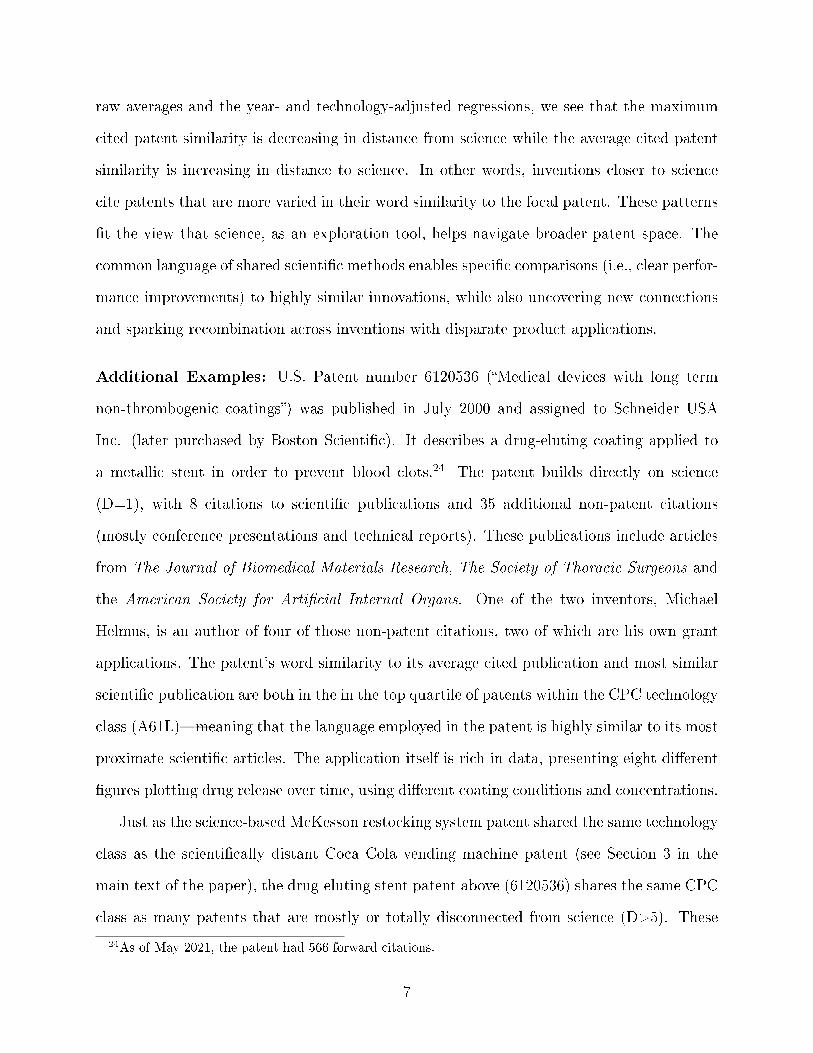
raw averages and the year- and technology-adjusted regressions, we see that the maximum

cited patent similarity is decreasing in distance from science while the average cited patent

similarity is increasing in distance to science. In other words, inventions closer to science

cite patents that are more varied in their word similarity to the focal patent. These patterns

�t the view that science, as an exploration tool, helps navigate broader patent space. The

common language of shared scienti�c methods enables speci�c comparisons (i.e., clear perfor-

mance improvements) to highly similar innovations, while also uncovering new connections

and sparking recombination across inventions with disparate product applications.

Additional Examples: U.S. Patent number 6120536 (�Medical devices with long term

non-thrombogenic coatings�) was published in July 2000 and assigned to Schneider USA

Inc. (later purchased by Boston Scienti�c). It describes a drug-eluting coating applied to

a metallic stent in order to prevent blood clots.24 The patent builds directly on science

(D=1), with 8 citations to scienti�c publications and 35 additional non-patent citations

(mostly conference presentations and technical reports). These publications include articles

from The Journal of Biomedical Materials Research, The Society of Thoracic Surgeons and

the American Society for Arti�cial Internal Organs. One of the two inventors, Michael

Helmus, is an author of four of those non-patent citations, two of which are his own grant

applications. The patent's word similarity to its average cited publication and most similar

scienti�c publication are both in the in the top quartile of patents within the CPC technology

class (A61L)�meaning that the language employed in the patent is highly similar to its most

proximate scienti�c articles. The application itself is rich in data, presenting eight di�erent

�gures plotting drug release over time, using di�erent coating conditions and concentrations.

Just as the science-based McKesson restocking system patent shared the same technology

class as the scienti�cally distant Coca Cola vending machine patent (see Section 3 in the

main text of the paper), the drug-eluting stent patent above (6120536) shares the same CPC

class as many patents that are mostly or totally disconnected from science (D>5). These

24As of May 2021, the patent had 566 forward citations.

7

include materials that prevent oxidation of medical implants (5543471, D=6), a �lm that

shrinks upon contact with excess water (patent number 5641562, D=5), and air �lters which

contain tea extracts that might deactivate viruses (5747053, D=5). Clearly, all of the above

inventions bene�t indirectly from the scienti�c advances of the modern era from physics,

chemistry and microbiology. However, as applied engineering e�orts, their search process

and method for communicating the invention's distinctive features and value is di�erent

since they do not relate their work to formal scienti�c �ndings.

8

Nb. Family Nb. Days Claim ClaimPatents Year Size Inventors Processed Words App. Words Filed

Distance 1 234946 2001.8 6.23 2.89 1100.2 110.6 166.3Distance 2 386061 2001.9 4.13 2.64 1040.9 113.4 164.3Distance 3 240145 2000.9 3.93 2.54 923.2 122.8 167.1Distance 4 105705 1997.4 3.77 2.40 795.8 137.6 175.5Distance 5 60579 1994.0 3.54 2.23 728.4 141.4 181.6Distance >5 67355 1991.5 3.39 2.07 686.5 146.0 181.8Unconbected 40966 1989.2 3.51 2.05 701.5 144.0 171.1Total 1135757 1999.7 4.39 2.57 955.5 118.9 167.2

Table A.1: Patent Characteristics, by Distance to Science

Notes: Table A.1 presents patent characteristics for patents in the analysis sample, by degree of distance

from science.

Nb. Share Share StdDev. Max. Avg.Cites Self-Cites Same-Tech Age Age Sim. Cited Sim. Cited

Distance 1 13.3 0.14 0.54 8.00 5.27 0.55 0.31Distance 2 11.8 0.14 0.56 7.38 5.18 0.54 0.32Distance 3 9.77 0.17 0.56 8.33 6.10 0.52 0.34Distance 4 9.93 0.18 0.56 10.9 8.11 0.52 0.35Distance 5 10.7 0.16 0.57 12.9 9.44 0.50 0.35Distance >5 10.2 0.14 0.60 15.0 10.9 0.48 0.36Unconnected 8.58 0.13 0.59 22.0 12.7 0.44 0.37Total 11.2 0.15 0.56 9.18 6.38 0.53 0.33

Table A.2: Backward Citations, by Distance to Science

Table A.2 describes backwards citation characteristics for patents in the analysis sample, by degree of distance

from science.

9

(1) (2) (3) (4) (5) (6) (7) (8)Nb. Processing Claim Nb. Backwards Share Avg. Age Max. Avg.

Outcome: Inventors Days Words Cites Same-Tech Cites Sim. Cited Sim. Cited

Distance 1 0.329*** 101.1*** -13.54*** 6.47*** -0.055*** -0.59*** 0.054*** -0.037***(0.00706) (10.32) (0.878) (0.085) (0.0013) (0.024) (0.00078) (0.00055)

Distance 2 0.184*** 58.03*** -12.82*** 3.43*** -0.042*** -1.22*** 0.037*** -0.025***(0.00647) (9.445) (0.800) (0.078) (0.0012) (0.022) (0.00071) (0.00050)

Distance 3 0.0796*** -4.608 -9.634*** 1.62*** -0.024*** -1.12*** 0.0076*** -0.010***(0.00657) (9.598) (0.787) (0.079) (0.0012) (0.022) (0.00072) (0.00051)

Distance 5 -0.0220** 10.47 5.677*** -1.51*** 0.014*** 1.38*** -0.011*** 1.8e-06(0.00890) (13.00) (1.343) (0.11) (0.0016) (0.030) (0.00097) (0.00069)

Distance >5 -0.0494*** 16.15 6.206*** -3.74*** 0.050*** 2.87*** -0.023*** 0.0099***(0.00887) (12.96) (1.746) (0.11) (0.0016) (0.030) (0.00097) (0.00069)

Unconnected -0.0617*** 33.51** 1.343 -4.17*** 0.055*** 9.82*** -0.052*** 0.020***(0.0106) (15.47) (2.352) (0.13) (0.0022) (0.040) (0.0014) (0.00097)

Tech x Year FE Yes Yes Yes Yes Yes Yes Yes YesObservations 1,135,747 1,135,725 232,049 1,135,747 1,114,025 1,114,025 1,108,568 1,108,568

Table A.3: Patent Characteristics and Backwards Citations, by Distance to Science (Regres-sions)

Table A.3 presents OLS regression results of distance to science on a a variety of patent characteristics. In

each regression, the omitted group is patents where degree is equal to four (D=4). The outcome variable in

Column 1 is the number of inventors listed on the patent. In Column 2, the dependent variable is number

of days between a patent's �rst application and issuance. Columns 3 show results for number of words in

patents' �rst claim in the issued patent. Column 4's outcome is the total number of backwards citations to

other patents. Column 5 uses the share of each patent's backward citations that go to same (4-digit) CPC

technology class as the focal patent. Column 6 reports results for the average age of backwards citations.

Column 7 and 8's outcomes are the maximum and average similarity of the focal patent's text to the text

of it's cited patents. All models include patent issuance year and technology class (4-digit CPC code) �xed

e�ects. *** p<0.01, ** p<0.05, * p<0.1.

10

B Additional Regressions and Robustness Results

We further investigate the relationship between patent values and distance to science using

additional regression speci�cations.

B.1 Patent Value Outcomes (in Levels), by Distance to Science and

Text Similarity

Columns 1�3 of Appendix Table A.5 are analogous to those Table 1, but with coe�cients

that correspond to level di�erences rather than percentage di�erences. This table generates

the patent value magnitudes that we report in Section 4.1. We report the same estimates as

Table 1 for Columns 4�6, which show the patent scope and litigation outcomes as alternative

measures of value. Appendix Table A.5 also has two additional Columns (7 and 8) which

report the text similarity between the focal patent and it's most similar scienti�c journal

articles as described above in Appendix A.1 and B.4.

11

B.2 Di�erent assumptions for KPSS value estimates

This section shows the sensitivity of our patent value measures to di�erent assumptions

about probability of patent grant. Our primary measure of patents' private value is from

Kogan et al. (2017) [KPSS]. While we primarily use the KPSS values as a measure of relative

value across distance from science and novelty groups (e.g., see Figure 1 and Table 1), we

also report dollar magnitudes adjusted for conservative estimates of patent grant rates (see

Section 4.1). An important assumption in the KPSS patent valuation method is choosing

the value for a patent's ex-ante probability of success, π. Using a higher probability of patent

success mechanically increases all patent values since the method scales all patent values by

(1− π)−1. The intuition is that a big positive stock market response is even more indicative

of a valuable patent is the market was already expecting that the patent had a decent chance

of approval.

Appendix Table A.4 shows how various adjustments to the KPSS values change the dollar

magnitudes of average patent values by distance to science. Columns 1 and 2 of Appendix

Table A.4 report the average patent values, by distance to science, based on the adjusted

values used throughout the main body of the paper, without and with technology × year

�xed e�ects. As described in Section 4.1, these �new baseline� estimates de�ate all KPSS

values by 12% to match the most conservative end of the spectrum for probability of patent

grant. In other words, conditional on the market being aware of a patent application, we

assume the greatest average market �surprise� for patent publication events. For contrast,

Columns 4 and 5 show the same regressiosn using the undadjusted (�old baseline�) KPSS

values.

Columns 5 and 6 use a more extreme adjustment: assuming that the market had no

information about a patent application prior to patent publication. This alternative shows

a 40%-50% drop in average patent values with this approach [Column (1) vs. Column (5)],

but the general relationship between distance from science and relative value holds. We

think this additional analysis is useful for o�ering a sort of lower-bound, however reality

12

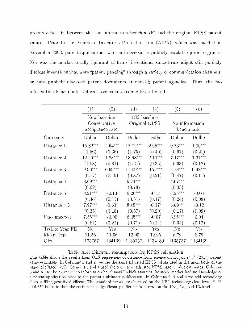
probably falls in between the �no information benchmark� and the original KPSS patent

values. Prior to the American Inventor's Protection Act (AIPA), which was enacted in

November 2002, patent applications were not necessarily publicly available prior to grants.

Nor was the market totally ignorant of �rms' inventions, since �rms might still publicly

disclose inventions that were �patent pending� through a variety of communication channels,

or have publicly disclosed patent documents at non-US patent agencies. Thus, the �no

information benchmark� values serve as an extreme lower bound.

(1) (2) (3) (4) (5) (6)

New baseline Old baselineConservative Original KPSS No information

acceptance rate benchmark

Outcome: Dollar Dollar Dollar Dollar Dollar Dollar

Distance 1 15.82∗∗∗ 2.64∗∗∗ 17.72∗∗∗ 2.95∗∗∗ 9.73∗∗∗ 1.90∗∗∗

(1.56) (0.36) (1.75) (0.40) (0.97) (0.21)Distance 2 12.49∗∗∗ 1.88∗∗∗ 13.98∗∗∗ 2.10∗∗∗ 7.47∗∗∗ 1.31∗∗∗

(1.08) (0.31) (1.21) (0.35) (0.68) (0.18)Distance 3 9.90∗∗∗ 0.69∗∗∗ 11.09∗∗∗ 0.77∗∗∗ 5.78∗∗∗ 0.48∗∗∗

(0.77) (0.19) (0.87) (0.21) (0.47) (0.11)Distance 4 8.69∗∗∗ 9.74∗∗∗ 4.67∗∗∗

(0.62) (0.70) (0.33)Distance 5 8.21∗∗∗ -0.13 9.20∗∗∗ -0.15 4.25∗∗∗ -0.04

(0.46) (0.15) (0.51) (0.17) (0.24) (0.08)Distance >5 7.27∗∗∗ -0.33∗ 8.15∗∗∗ -0.37∗ 3.69∗∗∗ -0.12

(0.33) (0.18) (0.37) (0.20) (0.17) (0.09)Unconnected 7.55∗∗∗ -0.06 8.45∗∗∗ -0.07 3.85∗∗∗ 0.04

(0.64) (0.22) (0.71) (0.24) (0.34) (0.12)Tech x Year FE No Yes No Yes No YesMean Dep. 11.56 11.56 12.95 12.95 6.79 6.79Obs. 1135757 1134139 1135757 1134139 1135757 1134139

Table A.4: Di�erent assumptions for KPSS calculationThis table shows the results from OLS regressions of distance from science on Kogan et al. (2017) patentvalue estimates. In Columns 1 and 2, we use the same adjusted KPSS values used in the main body of thepaper (de�ated 12%). Columns 3 and 4 used the original unadjusted KPSS patent value estimates. Columns5 and 6 use the extreme �no information benchmark� which assumes the stock market had no knowledge ofa patent application prior to the patent's ultimate publication. In Columns 2, 4 and 6 we add technologyclass × �ling year �xed e�ects. The standard errors are clustered on the CPC technology class level. *, **and *** indicate that the coe�cient is signi�cantly di�erent from zero on the 10%, 5%, and 1% level.

13

B.3 Split by technology

One concern might be that the observed e�ects are driven by a single technology that bene�ts

particularly from science. This is not the case. In Figure A.2, we show the main graph

separately for broad technology categories measured by one-digit CPC classes. Panels (a)

and (b) show the raw data. In Panels (c) and (d) we normalize by the average values

of patents in the same four-digit CPC technology classi�cation and �ling year. For all

technologies, there is a decrease in value by distance to science, most pronounced for drugs

and chemicals. Results by other technology classi�cations such as the classi�cation in Hall

et al. (Hall et al., 2001) and Schmoch (Schmoch, 2008) are available from the authors on

request.

14

-60%

-40%

-20%

0%

20%

40%

60%

80%

100%


Distance to science

A Human necessitiesB Performing operationsC ChemistryD Textiles; paper


(a) Value by broad patent class A-D

-20%

0%

20%

40%


Distance to science

A Human necessitiesB Performing operationsC ChemistryD Textiles; paper


(b) Accounting for technology× year

-40%

-20%

0%

20%

40%

60%

80%

100%

120%

140%


Distance to science

E Fixed constructionsF Mechanical engineeringG PhysicsH Electricity


(c) Value by broad patent class E-G

-20%

0%

20%

40%

60%

80%


Distance to science

E Fixed constructionsF Mechanical engineeringG PhysicsH Electricity


(d) Accounting for technology × year

Figure A.2: Sample splits by technology

In this �gure, we split patents by broad technology �elds measured by one-digit CPC classes. In Panels (a)and (c) we show the raw data. In Panels (b) and (d) we normalize by the average patent value of a patentin the same four-digit CPC class and �ling year with a distance of four.

15

B.4 Comparing Patent and Scienti�c Article Text

One potential concern one might have about our estimation of the science premium of patents

is that the distance to science calculated by citations might measure not only how much a

patent uses science but also the quality of the inventor. A high-quality inventor might be

more aware of scienti�c research and therefore include more citations, but without actually

using science.

To see whether patents close to science make use of its content, we compare the texts of

scienti�c articles and the text of patents. We calculate the pairwise text similarity between

a patent and the articles cited in the patent. Then we take the maximum over all the

similarities of a patent to its cited articles to determine the distance to the closest article.

To calculate the similarity between the abstracts of the article and of the patent we use the

�term frequency-inverse document frequency� (tf-idf) method.25

The results presented in Column 7 of Table A.5 show that patents with a citation distance

of D=1 have a higher text similarity to scienti�c articles than patents more distant to science.

This suggests that citation distance re�ects indeed how much a patent is related to science.

Consistent with the idea that patents with more scienti�c content have a higher value,

Column 8 shows that the value of a patent increases with its text similarity to scienti�c

articles. This suggests that the relation between citation distance and patent value presented

as our main result above is not a result of a spurious correlation driven by third factors that

are unrelated to the scienti�c content of the patent.

B.5 Patent Tail Outcomes

Our primary regression results look at how average patent values vary with distance from

science (Table 1). However, as we see in Figure 1 (Panels (b) and (d)) The increase in

value due to science also comes with an increased likelihood of tail outcomes accounting

25We use the �gensim� implementation in Python for our calculations (see: https://radimrehurek.com/gensim/).

16

for technology and year. In Columns 5 and 6 of Appendix Table A.6, we investigate the

likelihood that a patent is in the top 5% or bottom 5% of the distribution of the science

component as an outcome. The distribution is taken over all patents. Patents that are closer

to science have a higher likelihood to be in the tails of this distribution. So, accounting for

the technological component, science-based patents show a larger variance in values.

17

B.6 E�ects over the entire value distribution

The main paper shows that average patent values decrease with distance to science relative

to the average value of a patent with the same �ling year and the same (four-digit) CPC technology

classi�cation with a distance of four. This pattern is already visible in the raw data in Figure

A.3a. In Figure A.3b we show the value by distance of science over the 25th, 50th and

75th percentile of the value distribution. We residualize each percentile with the same

percentile of patents with D=4.26 The patent values are falling with distance to science over

all percentiles. This con�rms that our results are not driven by outliers.

(a) Raw data

-2

0

2

4

6


Distance to science

p75p50p25

Percentiles

Average Dollar value in millions

(b) Value percentiles residualized with same percentilein D=4

Figure A.3: E�ects over the value distribution

Panel (a) shows the raw data for patent values by distance to science data for a 10% sample of patents. Thevalues of U.S. patents are from Kogan et al (Kogan et al., 2017). The distance to science of U.S. patents iscalculated with Marx and Fuegi Marx and Fuegi (2020) and Patstat using the method of Ahmadpoor andJones (Ahmadpoor and Jones, 2017). The distance to science is de�ned by citation links. A patent thatdirectly cites an academic article has a distance of D=1. A patent that cites a (D=1)-patent but not anacademic article has a distance of D=2. Patents are de�ned as �Unconnected� if there is no citation link toan academic article. In Panel (b), we show the average patent value for all distances to science along withthe number of patents in each distance. Panel (b) shows the 25th, 50th and 75th percentiles of the patentvalue distribution by distance to science normalized by its percentile at a distance of four.

26Here, we do not account for technology and year, as for many technology-�ling year combinations thereare not enough patents to obtain a distribution for every distance to science.

18

B.7 Patent value by distance to science and novelty

Distance to science and novelty are correlated, however within distance to science group, we

still observe variation in novelty of word combinations. This variation allows us to explore

how patent value di�ers if we turn novelty �on� or �o�.� In Appendix Figure A.4 we compare

patent values by both distance to science and novelty. Speci�cally, we regress patent value

on interactions between distance to science and an indicator for whether patents are below

or above median novelty. Novelty is measured by the likelihood of pairwise combinations of

words that occur in a particular patents after account for technology class and �ling year

(i.e., the same novelty measure as Figure 2, Panels (c) and (d)). In Appendix Figure A.4,

Panels (a) and (b) graph patent values as percentage di�erences relative to the (D=4), low

novelty group, with and without technology × year �xed e�ects. Panels (c) and (d) show the

equivalent regression results, but reporting coe�cients in levels (millions of $USD), rather

than percentage di�erences.

We discuss the results at the end of Section 4.3.

19

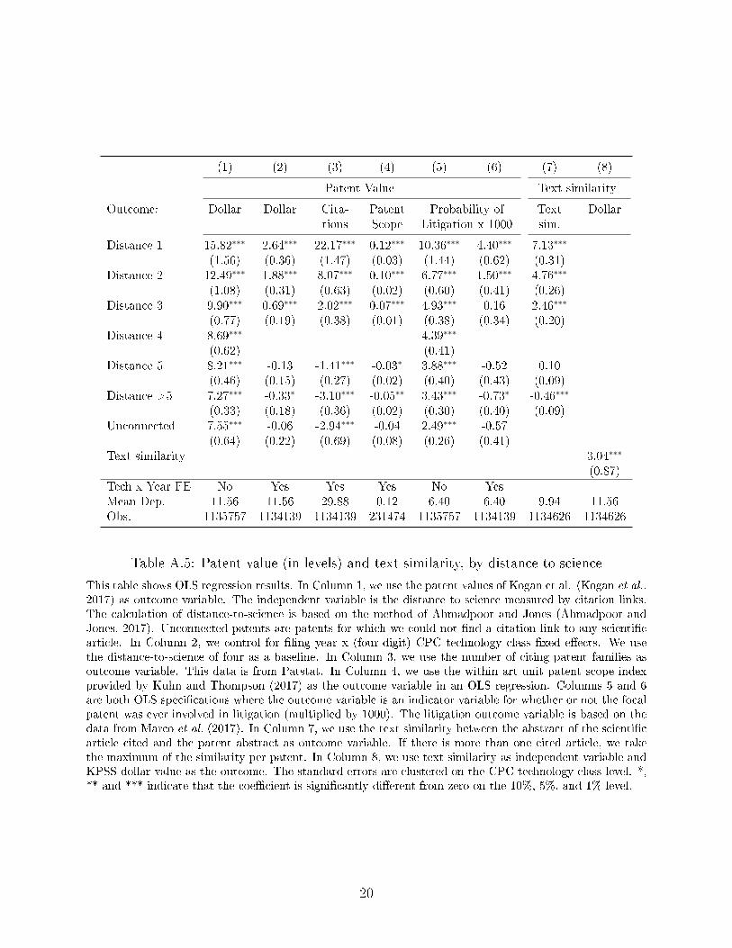
(1) (2) (3) (4) (5) (6) (7) (8)

Patent Value Text similarity

Outcome: Dollar Dollar Cita- Patent Probability of Text Dollartions Scope Litigation x 1000 sim.

Distance 1 15.82∗∗∗ 2.64∗∗∗ 22.17∗∗∗ 0.12∗∗∗ 10.36∗∗∗ 4.40∗∗∗ 7.13∗∗∗

(1.56) (0.36) (1.47) (0.03) (1.44) (0.62) (0.31)Distance 2 12.49∗∗∗ 1.88∗∗∗ 8.07∗∗∗ 0.10∗∗∗ 6.77∗∗∗ 1.50∗∗∗ 4.76∗∗∗

(1.08) (0.31) (0.63) (0.02) (0.60) (0.41) (0.26)Distance 3 9.90∗∗∗ 0.69∗∗∗ 2.02∗∗∗ 0.07∗∗∗ 4.93∗∗∗ 0.16 2.46∗∗∗

(0.77) (0.19) (0.38) (0.01) (0.38) (0.34) (0.20)Distance 4 8.69∗∗∗ 4.39∗∗∗

(0.62) (0.41)Distance 5 8.21∗∗∗ -0.13 -1.41∗∗∗ -0.03∗ 3.88∗∗∗ -0.52 0.10

(0.46) (0.15) (0.27) (0.02) (0.40) (0.43) (0.09)Distance >5 7.27∗∗∗ -0.33∗ -3.10∗∗∗ -0.05∗∗ 3.43∗∗∗ -0.73∗ -0.46∗∗∗

(0.33) (0.18) (0.36) (0.02) (0.30) (0.40) (0.09)Unconnected 7.55∗∗∗ -0.06 -2.94∗∗∗ -0.04 2.49∗∗∗ -0.57

(0.64) (0.22) (0.69) (0.08) (0.26) (0.41)Text similarity 3.04∗∗∗

(0.87)Tech x Year FE No Yes Yes Yes No YesMean Dep. 11.56 11.56 29.88 0.12 6.40 6.40 9.94 11.56Obs. 1135757 1134139 1134139 231474 1135757 1134139 1134626 1134626

Table A.5: Patent value (in levels) and text similarity, by distance to science

This table shows OLS regression results. In Column 1, we use the patent values of Kogan et al. (Kogan et al.,2017) as outcome variable. The independent variable is the distance to science measured by citation links.The calculation of distance-to-science is based on the method of Ahmadpoor and Jones (Ahmadpoor andJones, 2017). Unconnected patents are patents for which we could not �nd a citation link to any scienti�carticle. In Column 2, we control for �ling year x (four-digit) CPC technology class �xed e�ects. We usethe distance-to-science of four as a baseline. In Column 3, we use the number of citing patent families asoutcome variable. This data is from Patstat. In Column 4, we use the within art unit patent scope indexprovided by Kuhn and Thompson (2017) as the outcome variable in an OLS regression. Columns 5 and 6are both OLS speci�cations where the outcome variable is an indicator variable for whether or not the focalpatent was ever involved in litigation (multiplied by 1000). The litigation outcome variable is based on thedata from Marco et al. (2017). In Column 7, we use the text similarity between the abstract of the scienti�carticle cited and the patent abstract as outcome variable. If there is more than one cited article, we takethe maximum of the similarity per patent. In Column 8, we use text similarity as independent variable andKPSS dollar value as the outcome. The standard errors are clustered on the CPC technology class level. *,** and *** indicate that the coe�cient is signi�cantly di�erent from zero on the 10%, 5%, and 1% level.

20

(1)

(2)

(3)

(4)

(5)

(6)

(7)

(8)

PatentValue

PatentValuerelative

toD=4bytech

and�lingyear

Outcom

e:Probability

ofTop

5%Bottom

5%Top

5%Bottom

5%Top

5%Bottom

5%Top

5%Bottom

5%

Distance

17.8∗

∗∗3.1∗

∗∗1.3∗

∗∗-0.6

∗∗

(1.1)

(0.5)

(0.2)

(0.2)

Distance

25.5∗

∗∗4.8∗

∗∗0.9∗

∗∗-0.5

∗∗∗

(0.6)

(0.5)

(0.2)

(0.2)

Distance

34.1∗

∗∗6.6∗

∗∗0.3∗

∗-0.3

∗∗∗

(0.4)

(0.6)

(0.1)

(0.1)

Distance

43.3∗

∗∗6.2∗

∗∗

(0.3)

(0.7)

Distance

52.7∗

∗∗5.6∗

∗∗-0.0

0.1

(0.2)

(0.8)

(0.1)

(0.1)

Distance

>5

2.0∗

∗∗5.3∗

∗∗-0.2

0.2∗

∗

(0.2)

(0.8)

(0.1)

(0.1)

Unconnected

2.2∗

∗∗4.0∗

∗∗0.0

0.3∗

∗∗

(0.3)

(0.5)

(0.1)

(0.1)

Probability

ofword

combinations

-26.7∗

∗∗25.1

∗∗∗

-4.8

∗∗∗

1.0∗

∗

(2.7)

(4.5)

(0.8)

(0.5)

MeanDep.

5.00

5.00

5.00

5.00

5.00

5.00

5.00

5.00

Obs.

1135757

1135757

1135669

1135669

1135757

1135757

1135669

1135669

TableA.6:Distribution

ofpatentvalue

Thistableshow

sthedistributionofpatentvalues

bydistance

toscience

andbypatentnovelty.In

columns1and3,weuse

thepatentvalues

ofKogan

etal.(K

oganet

al.,2017)to

assignto

each

patentanindicatorequalto

oneifitsvalueisin

thetop5%

ofallpatentvalues.In

columns2and4,

weassignanindicatorequalto

oneifthepatentisin

thebottom

5%

ofthepatentvaluedistribution.In

columns1and2,theindependentvariable

isthedistance

toscience

measuredbycitationlinks.

Unconnectedpatents

are

patents

forwhichwecould

not�ndacitationlinkto

anyscienti�c

article.In

columns3and4,weuse

anovelty

indicator-theaverageprobabilityof2-tupleword

combinationofeach

patent-asanoutcomevariable.

Incolumns5to

8,weuse

insteadofthedistributionofallpatentvalues

thedistributionofthescience

valuecomponentto

calculate

thetopand

bottom

5%

ofthedistribution.Thescience

valuecomponentisderived

bycalculatingtheresidualofthepatentvalueandtheaveragepatentvalue

ofapatentin

thesametechnologyandyearwithadistance

offour.

Thestandard

errors

are

clustered

ontheCPCtechnologyclass

level.*,**and

***indicate

thatthecoe�

cientissigni�cantlydi�erentfrom

zero

onthe10%,5%,and1%

level.

21

-20%

0%

20%

40%

60%

80%

100%

120%


Distance to science

Below median noveltyAbove median novelty


(a) % di�erences

-10%

0%

10%

20%

30%


Distance to science



(b) % di�erence, accounting for tech and year

0

5

10

15

20


Distance to science

Below average noveltyAbove average novelty


(c) Averages ($ levels)

0

1

2

3

4


Distance to science


Average difference in value in millions $USD than patents with D=4in same technology class and with the same filing year

(d) $ level di�erences, accounting for tech and year

Figure A.4: Patent value by distance from science and novelty

Panel (a) shows the average patent value for all distances to science relative to patents with a distance of(D=4), and separates by patents with above and below median novelty. Novelty is measured by the likelihoodof pairwise combinations of words that occur in a particular patents and we account for technology classand �ling year. The values of U.S. patents are from Kogan et al. (Kogan et al., 2017). The distance toscience of U.S. patents is calculated with Microsoft Academic and Patstat using the method of Ahmadpoorand Jones (Ahmadpoor and Jones, 2017). The distance to science is de�ned by citation links. The 90%con�dence bounds are based on standard errors clustered by (four-digit) CPC technology class. In Panel (b),we residualize the patent value by the average value of a patent with the same (four-digit) CPC technologyclass and �ling year and a distance of four. We again plot seperate values for patents with above and belowaverage novelty. Panel (c) shows the average dollar value of patents in levels for all distances to science forboth below and above average novelty patents. Panel (d) residualizes dollar patent values by the averagevalue of a patent with the same (four-digit) CPC technology class and �ling year and a distance of four.

22

C Alternative data and method choices

In this section, we discuss the results using alternative data and methodological choices.

C.1 Using Ahmadpoor and Jones distance values

In Figures A.5a and A.5b, we use the distance-to-science measure based on the data of

Ahmadpoor and Jones (Ahmadpoor and Jones, 2017). The data of Ahmadpoor and Jones

(Ahmadpoor and Jones, 2017) is based on Web of Science while our measure is based on

the data of Microsoft Academic. There are two main di�erences. First, Ahmadpoor and

Jones (Ahmadpoor and Jones, 2017) have many more unconnected patents (165 thousand

unconnected patents out of 0.8 million overall patents) than we do (54 thousand unconnected

patents out of 1.1 million overall patents). Second, we aggregate the patents with a distance

larger than 5 as the number of patents goes down dramatically for larger distances. We �nd

the same overall pattern; i.e., the patent values decrease in percent relative to D=4 with

distance to science.

23

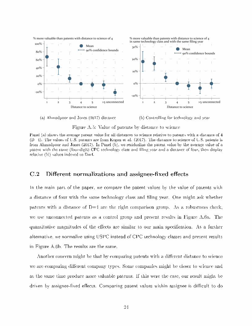
-20%

0%

20%

40%

60%

80%

100%


Distance to science



(a) Ahmadpoor and Jones (2017) distance

-10%

0%

10%

20%

30%


Distance to science



(b) Controlling for technology and year

Figure A.5: Value of patents by distance to science

Panel (a) shows the average patent value for all distances to science relative to patents with a distance of 4(D=4). The values of U.S. patents are from Kogan et al. (2017). The distance to science of U.S. patents isfrom Ahmadpoor and Jones (2017). In Panel (b), we residualize the patent value by the average value of apatent with the same (four-digit) CPC technology class and �ling year and a distance of four, then displayrelative (%) values indexed to D=4.

C.2 Di�erent normalizations and assignee-�xed e�ects

In the main part of the paper, we compare the patent values by the value of patents with

a distance of four with the same technology class and �ling year. One might ask whether

patents with a distance of D=4 are the right comparison group. As a robustness check,

we use unconnected patents as a control group and present results in Figure A.6a. The

quantitative magnitudes of the e�ects are similar to our main speci�cation. As a further

alternative, we normalize using USPC instead of CPC technology classes and present results

in Figure A.6b. The results are the same.

Another concern might be that by comparing patents with a di�erent distance to science

we are comparing di�erent company types. Some companies might be closer to science and

at the same time produce more valuable patents. If this were the case, our result might be

driven by assignee-�xed e�ects. Comparing patent values within assignee is di�cult to do

24

with the Kogan et al. (Kogan et al., 2017) data. The reason is that all patents published by

the same assignee at the same date have the same value as their evaluation is based on the

same abnormal stock market returns. This is why for this exercise we use forward citations

as an outcome variable. In Figure A.6c, we normalize the number of forward citations by

each combination of assignee, �ling year and technology class. This implies that we look

only at citation di�erences within the same assignee. We �nd the same pattern as in our

main result.

25

-10%

0%

10%

20%

30%


Distance to science


% more valuable than unconnected patentsin same technology class and with the same filing year

(a) Relative to unconnected

-10%

0%

10%

20%

30%


Distance to science



(b) Based on USPC instead of CPC-technology class

-10%

0%

10%

20%

30%

40%

50%

60%

70%

80%


Distance to science


% more forward citations than patents with distance to science of 4in same technology class and with the same filing year and assignee

(c) Forward citations and assignee �xed e�ect

Figure A.6: Di�erent normalizations and assignee-�xed e�ects

Panel (a) shows the average value of patents normalized by the value of patents that were �led in the sameyear but are unconnected to science. Panel (b) shows results using USPC patent classes instead of CPCpatent classes. In Panel (c), we use forward citations instead of patent values as the outcome and adjust forassignee-�xed e�ects.

26

C.3 Number of citations to science and value

Our primary measure of distance to science does not account for the intensity of citations to

science. A patent that cites one single scienti�c article and a patent citing dozens of journal

articles both end up in the (D=1) group. To investigate whether the number of citations to

scienti�c articles is correlated with patents' private value, we use number of cited articles as

an alternative distance to science measure.

Appendix Figure A.7 shows the results of this analysis. Both panels graph Kogan et al.

(2017) values for di�erent numbers of citations to scienti�c articles. The size of each obser-

vation circle is proportional to the number of observations for each value of �number of cited

articles.� The modal patent has no citations to science. Panel (a) displays the raw averages

and shoes a fairly steady increase in average value as the number of cited articles increase.

In Panel (b), we residualize values using the average value of patents in the same tech-

nology class and �ling year. The residualized values show a similar pattern up until seven

cited articles, after which the values move more erratically. Notably, patents with more than

10 cited articles have an average value closest to patents with merely one scienti�c citation.

We cannot pinpoint the exact reason for the drop o� in residualized values beyond 10

citations, but we can speculate. Within some technology classes, a large number of scien-

ti�c citations may be indicative of a patent being a more incremental innovation. Relying

extensively on a series of past discoveries could mean that the patent is situated in a more

mature and crowded technological space. While reliance on science is generally valuable in

those technology classes, excessive citations might signal a narrowness or lack of novelty that

reduces the patent's private value. Such a pattern is in line with Krieger et al. (2021), who

�nd that drug candidates that are highly similar in structure to prior drugs have lower KPSS

patent values.

More generally, the number of scienti�c cites among the (D=1) is a noisy measure of how

reliant a paper is on science. Some sub�elds simply have a norm of more citations Marx and

Fuegi (2020). Additional citations in those �elds are more likely to be ceremonial in nature.

27

In such high citation scienti�c areas, we do not expect more citations to correlate with higher

private value, nor relying any more on science than in areas where citing patterns are more

selective.

8

10

12

14

16

18

20

22

0 1 2 3 4 5 6 7 8 9 10 >10

Number of cited articles


(a) Averages

0

1

2

3

4

5

0 1 2 3 4 5 6 7 8 9 10 >10

Number of cited articles

Average value in millions $USDcontrolling for technology class and filing year

(b) Averages accounting for technology and year

Figure A.7: Number of articles cited and patent values

Panel (a) shows the average patent value and patents are split by the number of scienti�c articles cited inthe patent. The data on non-patent citations is from Marx and Fuegi (2020). In Panel (b), we residualizethe patent value by the average value of a patent with the same (four-digit) CPC technology class and �lingyear and a distance of four.

28

C.4 Alternative measures for novelty

New words and word age

In our main speci�cation, we measure how likely or unlikely the word combinations used in

a patent are to determine the novelty of a patent. In Figures A.8a and A.8b, we use the

data of Arts et al (Arts et al., 2018) to calculate two alternatives measures for novelty. The

�rst measure indicates whether a patent has a new word. A word is new if it was not used in

any patent before. Figure A.8a shows that the share of patents with a new word decreases

monotonically with its distance to science. The second measure is the average age of words

used in a patent. We calculate the age of a word by calculating the di�erence between the

�ling year and the �ling year of the patent in which it was �rst used. The average word age

is systematically lower for patents that are closer to science (Figure A.8b). If word age is

indicative for the age of the ideas they encode, patents closer to science contain more novel

ideas.

Both of the alternative novelty measures are positively related to patent value. Figure

A.8c compares the patent value for patents with and without new words for each year,

controlling for technology × year �xed e�ects. From 1980�1998, we see that patents with

new words have a positive (average) value premium over those without new words. Then,

from 1998�2000, patents with new words are actually less valuable on average. Presumably

this period featured a lot of highly valued, but (relatively) low novelty software patents

without new words. Firms may have been able to capture value from �jumping on the

bandwagon� with software patents in that brief period, but the �bursting� of the dot com

bubble in 2000 suggests that many of those software patents were indeed overvalued in the

longer run.

Figure A.8d shows the relation between the average age of words of a patent relative to

the year and technology class and the residualized patent value. We see a negative relation

between patent value and the average age of words.

29

Chemical Patents and Compound Novelty

A potential shortcoming of measuring novelty with text analysis is that inventors and patent

lawyers have many degrees of freedom in choosing words. Word or word combination novelty

might re�ect the author's preferences or popular tech buzzwords, moreso than innate qual-

ities of the invention. Endogenous language choices might erroneously hide or suggest true

novelty (e.g., consider the use and abuse of word combinations involving terms like �crypto�

and �arti�cial intelligence� over time). To avoid the pitfalls of using language to measure

novelty, ideally innovation scholars would have standardized and quanti�able measures of

technological similarity for all technology classes over time.

While such standardized novelty measures do not exist for most technologies, chemical

patents allow for such structured measures of invention qualities. We use the crosswalk of

patents-to-compounds from SureChEMBL, which extracts the standardized (SMILES code)

chemical structures represented in patents.27 Patents often have more than one chemical

described in their claims, and these chemicals need not be the central component of the the

new invention.

One way that chemists quantify the similarity of two given molecules is to calculate their

share of overlapping fragments as a �Tanimoto� (or Jaccard) chemical similarity score from

zero (no overlap) to one (total overlap). Using the general approach described in Krieger

et al. (2021) and with the aid of the ChemmineR package (Backman et al., 2011), we calculate

all the maximum pairwise (backwards) similarity between each of the compounds in a given

patent and all previously patented chemicals from the same 3-digit CPC class. The average

maximum similarity to prior patent chemicals is 0.86 with a median of 1. This general lack of

novelty is unsurprising since patents contain multiple compounds and inventive novelty might

come from recombination of existing compounds or complementary technologies claimed by

the patent. Thus, our chemical similarity measure is a conservative measure of novelty.

27The data includes 187,958,584 patent-compound pairs from 1960�2014. For more information on thedata see: http://chembl.blogspot.com/2015/03/the-surechembl-map-file-is-out.html.

30

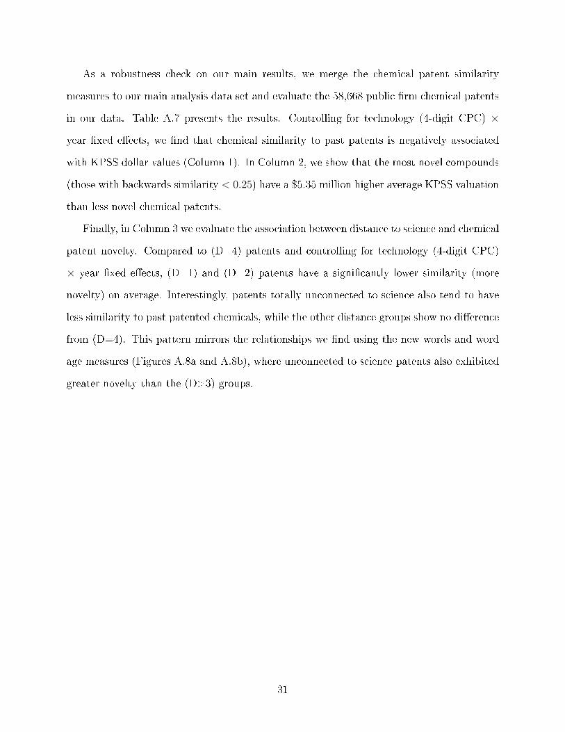
As a robustness check on our main results, we merge the chemical patent similarity

measures to our main analysis data set and evaluate the 58,668 public �rm chemical patents

in our data. Table A.7 presents the results. Controlling for technology (4-digit CPC) ×

year �xed e�ects, we �nd that chemical similarity to past patents is negatively associated

with KPSS dollar values (Column 1). In Column 2, we show that the most novel compounds

(those with backwards similarity < 0.25) have a $5.35 million higher average KPSS valuation

than less novel chemical patents.

Finally, in Column 3 we evaluate the association between distance to science and chemical

patent novelty. Compared to (D=4) patents and controlling for technology (4-digit CPC)

× year �xed e�ects, (D=1) and (D=2) patents have a signi�cantly lower similarity (more

novelty) on average. Interestingly, patents totally unconnected to science also tend to have

less similarity to past patented chemicals, while the other distance groups show no di�erence

from (D=4). This pattern mirrors the relationships we �nd using the new words and word

age measures (Figures A.8a and A.8b), where unconnected to science patents also exhibited

greater novelty than the (D>3) groups.

31

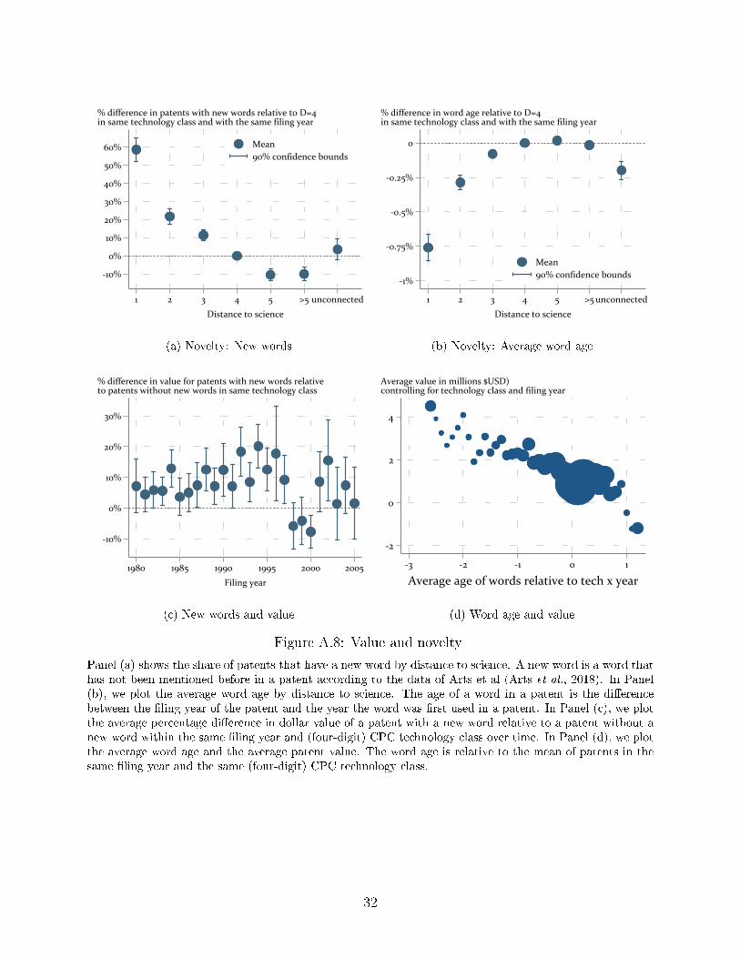
-10%

0%

10%

20%

30%

40%

50%

60%


Distance to science


% difference in patents with new words relative to D=4in same technology class and with the same filing year

(a) Novelty: New words

-1%

-0.75%

-0.5%

-0.25%

0


Distance to science


% difference in word age relative to D=4in same technology class and with the same filing year

(b) Novelty: Average word age

-10%

0%

10%

20%

30%

1980 1985 1990 1995 2000 2005

Filing year

% difference in value for patents with new words relativeto patents without new words in same technology class

(c) New words and value

-2

0

2

4

-3 -2 -1 0 1

Average age of words relative to tech x year

Average value in millions $USD)controlling for technology class and filing year

(d) Word age and value

Figure A.8: Value and novelty

Panel (a) shows the share of patents that have a new word by distance to science. A new word is a word thathas not been mentioned before in a patent according to the data of Arts et al (Arts et al., 2018). In Panel(b), we plot the average word age by distance to science. The age of a word in a patent is the di�erencebetween the �ling year of the patent and the year the word was �rst used in a patent. In Panel (c), we plotthe average percentage di�erence in dollar value of a patent with a new word relative to a patent without anew word within the same �ling year and (four-digit) CPC technology class over time. In Panel (d), we plotthe average word age and the average patent value. The word age is relative to the mean of patents in thesame �ling year and the same (four-digit) CPC technology class.

32

(1) (2) (3)Outcome: Dollars Dollars Chemical Similarity

Chemical Similarity -4.85**(2.36)

Most Novel Compounds 5.35***(1.99)

Zero Novelty Compounds -0.48(0.74)

Distance 1 -0.037***(0.014)

Distance 2 -0.012*(0.0069)

Distance 3 -0.00081(0.0044)

Distance 5 0.0052(0.0058)

Distance >5 -0.0012(0.0060)

Unconnected -0.060***(0.020)

Tech x Year FE Yes Yes YesObservations 60,009 60,009 60,009

Table A.7: Chemical novelty, patent value and distance to science

Notes: Table A.7 presents OLS regressions for the subset of patents associated with one or more chemical

structure. The patent to chemical crosswalk comes from SureChEMBL (www.surechembl.org), and chemical

similarity is calculated from zero (no similarity) to one (total structural overlap) based on Tanimoto scores.

Most novel compound patents are those with at least one compound with a maximum chemical similarity

to previously granted patents of zero or less than 0.25. Zero novelty compounds patents are those which

have no compounds with a backwards similarity less than 1. The omitted category is for patents with

between 0.25 and 0.99 chemical similarity to prior patents. The dependent variable in Columns 1 and 2 is

the (adjusted) KPSS patent dollar value. Column 3 presents the correlations between distance to science

and patent maximum chemical similarity to prior patented chemicals. All models have technology (4-digit

CPC) × year �xed e�ects. *** p<0.01, ** p<0.05, * p<0.1.

33

standing on the shoulders of science

Documents