standard for terrestrial ecosystem mapping in british columbia · standard for terrestrial...
TRANSCRIPT

Standard forTerrestrial Ecosystem Mappingin British Columbia
Prepared byEcosystems Working Group
Terrestrial Ecosystems Task ForceResources Inventory Committee
May 1998

© The Province of British ColumbiaPublished by theResources Inventory Committee
Canadian Cataloguing in Publication Data
Main entry under title:
Standard for terrestrial ecosystem mapping in British Columbia[computer file]
Available through the Internet.Issued also in printed format on demand.Includes bibliographical references: p.ISBN 0-7726-3552-8
1. Environmental mapping - Standards - British Columbia. 2.Biotic communities - British Columbia. 3. Ecological surveys -Standards - British Columbia. I. Resources Inventory Committee(Canada). Ecosystems Working Group.
QH541.15S95S73 1998 577'.09711 C98-960125-0
Additional Copies of this publication can be purchased from:
Superior Repro#200–1112 West Pender StreetVancouver, BC V6E 2S1Tel: (604) 683-2181Fax: (604) 683-2189
Digital Copies are available on the Internet at:
http://www.for.gov.bc.ca/ric

Abstract
May 1998 iii
Abstract
This report describes British Columbia standards for ecosystem mapping at scales of 1:5000 to1:50 000. The information here has been developed for, and approved by, the ResourcesInventory Committee (RIC), a provincial committee responsible for developing inventorystandards for the province.
These mapping standards use a three-level classification hierarchy of ecological units,including ecoregion units and biogeoclimatic units at broader levels, and site units andvegetation developmental stages (combined as ecosystem units) at a more detailed scale.Ecoregion classification is hierarchical, with five levels of generalization; the lowest level,ecosection, is used here. Biogeoclimatic classification includes four levels, including zone,subzone, variant, and phase. Ecoregion and biogeoclimatic units are broad-level delineationsderived from provincial maps. Within these broader units, site-level polygons describeecosystem units composed of site series, site modifiers, and structural stages.
At the first stage of ecosystem mapping, ecosystem units are delineated on aerial photographsfollowing a bioterrain approach. To draw and label polygons, the mapper considersvegetation, topographic, and terrain (surficial geology) features. Site, vegetation and terrainattributes are recorded in a polygon database, and final map completed. The polygons aredigitized and compiled in a geographic information system, and stored in a provincial database.
Outlined here are the standards established for ecosystem unit characterization, symbology,sampling, mapping procedures, interpretations and legends. Core data attributes to be collectedfor all ecosystem mapping projects in British Columbia are also described, in addition to otherattributes that are recommended in order to support interpretations for various landmanagement activities.

Standard for Terrestrial Ecosystem Mapping
iv May 1998

Acknowledgments
May 1998 v
Acknowledgments
Funding of the Resources Inventory Committee work, including the preparation of thisdocument, is provided by the Corporate Resource Inventory Initiative (CRII) and by ForestRenewal BC (FRBC). Preliminary work of the Resources Inventory Committee was fundedby the Canada-British Columbia Partnership Agreement of Forest Resource DevelopmentFRDA II.
The Resources Inventory Committee consists of representatives from various ministries andagencies of the Canadian and the British Columbia governments as well as from First Nationspeoples. RIC objectives are to develop a common set of standards and procedures for theprovincial resources inventories, as recommended by the Forest Resources Commission in itsreport “The Future of our Forests.”
For further information about the Resources Inventory Committee and its various TaskForces, please contact:
The Executive SecretariatResources Inventory Committee840 Cormorant StreetVictoria, BC V8W 2R1
Tel: (250) 920-0661Fax: (250) 384-1841
http://www.for.gov.bc.ca/ric
Terrestrial Ecosystem Task Force
This report was developed by the Ecosystems Working Group, part of the TerrestrialEcosystems Task Force under the Resources Inventory Committee (RIC). Substantialcontributions for this report have been provided by Barbara von Sacken, Robert Maxwell, TedLea, and Carmen Cadrin of the BC Ministry of Environment, Lands and Parks, and DelMeidinger and Allen Banner of the BC Ministry of Forests. Corey Erwin, Jo-Anne Stacey,and Tracy Fleming assisted with final preparation of the document. Richard Sims ofGeomatics International provided materials on map reliability, assessment, and qualityassurance. Many discussions were held and comments received from Ministry of ForestsRegional Ecologists Tom Braumandl, Ray Coupé, Craig DeLong, Dennis Lloyd, FredNuszdorfer, and Ordell Steen. Thanks also go to participants (consultants, industry, andprovincial government personnel) at a November 1996 workshop in Victoria, BC, who aided infinalizing the standards. As well, many practitioners were originally consulted as to whatattributes were required for developing interpretations from ecosystem maps.
Appreciation goes to Georgina Montgomery for editing the text, TM Communications Inc. andDebbie Webb for graphics and desktop publishing, and to Louise Gronmyr, Christina Stewart,Claudia Jones and Jean Stringer for final edit changes. Appreciation also goes to Rick Pawlasand Sean LeRoy for their graphic and desktop publishing work on the original review draft.

Standard for Terrestrial Ecosystem Mapping
vi May 1998
This report has borrowed extensively from previous mapping methodology papers that arecited in the text. We would like to acknowledge the technical contributions of Bob Mitchell,Bob Green, Graeme Hope, Karel Klinka, Dennis Demarchi, Ted Lea, Mike Fenger, andAndrew Harcombe who documented previous methods for ecosystem mapping in BritishColumbia. We also acknowledge the co-operation and leadership of RIC co-chairs, DaveGilbert, Mike Bonnor, and Jim Mattison, and the Terrestrial Ecosystems Task Force co-chairs,Imre Spandli, Bruce Pendergast, and A.Y. Omule. The Ecosystems Working Group consistsof the following individuals: Allen Banner, Carmen Cadrin, Dave Campbell, David Kilshaw,Ted Lea, Herb Luttmerding, Barry McDougall, Shirley Mah, Robert Maxwell, Del Meidinger,and Barbara von Sacken.

Table of Contents
May 1998 vii
Table of Contents
ABSTRACT ................................................................................................................... iii
ACKNOWLEDGEMENTS ..............................................................................................v
TABLE OF CONTENTS ............................................................................................... vii
LIST OF TABLES .......................................................................................................... ix
LIST OF FIGURES..........................................................................................................x
1.0 INTRODUCTION.....................................................................................................1
2.0 CLASSIFICATION AND MAPPING CONCEPTS ...................................................5
2.1 Ecoregion Units ......................................................................................................6
2.2 Biogeoclimatic Units................................................................................................6
2.3 Ecosystem Units .....................................................................................................7
2.3.1 Site series.........................................................................................................8
2.3.2 Site modifiers....................................................................................................8
2.3.3 Vegetation developmental units..........................................................................9
2.4 Terrain Units ........................................................................................................ 10
3.0 MAPPING CONVENTIONS .................................................................................. 11
3.1 Ecoregion/Biogeoclimatic Units.............................................................................. 11
3.2 Ecosystem Units ................................................................................................... 12
3.2.1 Site series....................................................................................................... 13
3.2.2 Site modifiers.................................................................................................. 18
3.2.3 Vegetation developmental units........................................................................ 20
3.2.4 Alternate methods for assigning site modifiers and structural stage ..................... 25
3.2.5 Naming ecosystem units.................................................................................. 26
3.3 Ecosystem Map Units ........................................................................................... 26
3.4 Terrain and Soil Attributes ..................................................................................... 27
3.5 Polygon Boundaries............................................................................................... 27
3.6 Options for Ecoregion/Biogeoclimatic Map Unit Symbols ......................................... 27
3.7 Options for Ecosystem Map Unit Symbols .............................................................. 28
4.0 POLYGON DATA AND INTERPRETATIONS ..................................................... 29
4.1 Core Polygon Data................................................................................................ 30
4.2 Polygon Data for Additional Interpretations............................................................. 30

Standard for Terrestrial Ecosystem Mapping
viii May 1998
5.0 MAP LEGENDS..................................................................................................... 33
6.0 MAPPING AND FIELD SURVEY PROCEDURES................................................ 37
6.1 Project Planning.................................................................................................... 37
6.1.1 Defining objectives and developing a working plan ............................................ 37
6.1.2 Compiling existing data .................................................................................... 39
6.1.3 Conducting field reconnaissance ...................................................................... 39
6.1.4 Developing the working legend ........................................................................ 40
6.2 Pre-typing of Aerial Photographs ........................................................................... 41
6.2.1 Conducting initial ecoregion/biogeoclimatic mapping .......................................... 41
6.2.2 Conducting initial ecosystem mapping............................................................... 43
6.3 Field Sampling....................................................................................................... 47
6.3.1 Establishing survey intensity............................................................................. 47
6.3.2 Designing a sampling plan................................................................................ 50
6.3.3 Conducting field inspections and plot sampling................................................... 51
6.4 Data Synthesis and Analysis .................................................................................. 56
6.5 Final Mapping....................................................................................................... 56
6.6 Interpretive Mapping ............................................................................................. 58
6.7 Quality Assurance, Correlation, and Map Reliability................................................. 61
6.7.1 Quality assurance and correlation..................................................................... 61
6.7.2 Map reliability................................................................................................. 63
7.0 SUMMARY OF METHODS AND STANDARDS .................................................. 65
7.1 Summary.............................................................................................................. 65
7.2 TEM Standards..................................................................................................... 66
REFERENCES .............................................................................................................. 69
APPENDIX A: GLOSSARY......................................................................................... 75
APPENDIX B: DATA SOURCES ................................................................................ 89
APPENDIX C: NATURAL DISTURBANCE TYPES................................................... 99

List of Tables
May 1998 ix
List of TablesTable 3.1 Codes and definitions for non-vegetated, sparsely vegetated, and
anthropogenic units......................................................................................... 14
Table 3.2 Site modifiers for atypical conditions ................................................................ 18
Table 3.3 Structural stages and codes............................................................................. 21
Table 3.4 Stand structure modifiers and codes................................................................. 23
Table 3.5 Stand composition modifiers and codes ............................................................ 24
Table 3.6 Example seral community types for the BWBSmw2......................................... 25
Table 4.1 Core polygon attributes required for terrestrial ecosystem mapping .................... 31
Table 4.2 Possible Terrestrial Ecosystem Mapping interpretations andthe associated attributes.................................................................................. 32
Table 5.1 Minimum data to be included on map legends ................................................... 33
Table 6.1 Example working legend for mapping ecosystem units ...................................... 41
Table 6.2 Criteria for delineating ecosystem map units on aerial photographs..................... 46
Table 6.3 Survey intensity levels for ecosystem mapping.................................................. 48
Table 6.4 Field inspection density for selected survey intensity/map scale combinations...... 49
Table 6.5 Minimum data collection requirements for Ecosystem Field Forms (FS882) ........ 53
Table 6.6 Minimum data collection requirements for ground inspections ............................ 55
Table 6.7 Ratings table for site productivity of Dog Creek TEM project............................ 58
Table 6.8 Ratings table for Mountain Goat suitability........................................................ 60
Table 7.1 TEM standards manuals, field forms, databases, and training courses................. 66
Standard for Terrestrial Ecosystem Mapping
x May 1998
List of Figures
Figure 1.1 Hierarchy of ecological land classifications in British Columbia .............................2
Figure 2.1 Levels of ecosystem integration and classification in terrestrial ecosystem mapping.5
Figure 2.2 Hierarchy of TEM classification levels ...............................................................8
Figure 3.1 Symbols for Biogeoclimatic Units ..................................................................... 11
Figure 3.2 Symbols for Ecosection and Biogeoclimatic Units.............................................. 12
Figure 3.3 Symbology for Ecosystem Units....................................................................... 12
Figure 3.4 Example ecosystem map of Dog Creek............................................................ 12
Figure 3.5 RIC and Ministry of Forests Site Series codes................................................... 13
Figure 3.6 Use of site modifiers in mapping site series ....................................................... 20
Figure 3.7 Structural stage modifiers. ............................................................................... 24
Figure 3.8 Compound map units. ...................................................................................... 26
Figure 3.9 Standardized polygon boundary line weights. ..................................................... 27
Figure 4.1 Examples of possible interpretations from ecosystem map.................................. 29
Figure 5.1 Example of Map Legend ................................................................................. 35
Figure 6.1 Summary of mapping and field survey procedures ............................................. 38
Figure 6.2 Delineation of Alpine Tundra and parkland subzone ........................................... 42
Figure 6.3 Integrated delineation criteria for developing Ecosystem Map Unit polygons........ 44
Figure 6.4 A landscape profile for the ESSFwk1............................................................... 45
Figure 6.5 Site productivity interpretive map for portion of Dog Creek TEM project ............ 59
Figure 6.6 Habitat suitability interpretive map for Mountain Goat........................................ 61
1.0 Introduction
May 1998 1
1.0 Introduction
The purpose of this report is to provide standards for terrestrial ecosystem mapping (TEM) inBritish Columbia. These standards should be used for all medium- and large-scale ecologicalmapping projects, to ensure that a consistent approach is applied. Common scales ofecological mapping are 1:20 000 to 1:50 000, though larger scales—such as 1:10 000 or1:5000—may be carried out to support specific interpretations. This report is a product of theResources Inventory Committee (RIC), whose objective is to provide integrated standards forall resource inventories in the province.
Ecosystem mapping is the stratification of a landscape into map units, according to acombination of ecological features, primarily climate, physiography, surficial material,bedrock geology, soil, and vegetation. Ecosystem mapping provides:
• a biological and ecological framework for land management;
• a means of integrating abiotic and biotic ecosystem components on one map;
• basic information on the distribution of ecosystems from which managementinterpretations (e.g., broad-scale landscape planning, site-specific interpretations) can bedeveloped;
• a basis for rating values of resources or indicating sensitivities in the landscape;
• a historic record of ecological site conditions that can be used as a framework formonitoring ecosystem response to management; and
• a demonstration tool for portraying ecosystem and landscape diversity.
Ecosystem maps, along with associated interpretations, supply valuable information for manyuses, particularly planning resource allocation. The maps are used, for example, to meet manyForest Practices Code-related needs, including landscape unit planning, forest developmentplanning, range use planning and the development and application of biodiversity guidelines,riparian guidelines, and the proposed identified wildlife management strategy.
Data requirements are outlined for interpretations related to five broad subject areas: forestmanagement, range management, wildlife management, biodiversity management, andterrain/soils.
This methodology has evolved from two previous methods manuals produced by the Ministryof Forests (Mitchell et al., 1989) and the Ministry of Environment, Lands, and Parks(Demarchi et al., 1990), and recent experience with application of 1995 standards (RIC,1995). It builds on the collective experience with mapping and field methods that have beentested and proven effective in different parts of the province over the last 20 years.
The approach to the mapping described here combines aspects of the biogeoclimaticecosystem classification (BEC) of the Ministry of Forests with aspects of the ecoregionclassification of the Ministry of Environment, Lands, and Parks. Regional, local, anddevelopmental ecosystems from four classifications are mapped: ecoregion (ecoregion units),

Standard for Terrestrial Ecosystem Mapping
2 May 1998
zonal (biogeoclimatic units), site (site series), and vegetation developmental (structuralstages and seral community types). Figure 1.1 illustrates the relationship between thesefour classifications.
Figure 1.1 Hierarchy of ecological land classifications in British Columbia
Ecoregion and biogeoclimatic polygons represent broad level regional and climatic landscapeunits. Maps typically depict ecosections and biogeoclimatic zones, subzones, and variants.Within this framework, site level units, termed “ecosystem units,” are defined based on theintegration of vegetation, terrain (surficial material), topography and soil characteristics.Ecosystem units are generally derived from the site series classification within the BEC, bybeing further differentiated based on more specific site conditions (e.g., site modifiers ),structural developmental stages, and (sometimes) seral community types.

1.0 Introduction
May 1998 3
The ecosystem units are mapped using a bioterrain approach, a procedure that focuses onobservable site and biological features assumed to determine the function and distribution ofplant communities on the landscape. Map units are delineated using a combination ofaerial photograph interpretation and field sampling to verify ecosystem identificationand boundaries.
Presented here is information about terrestrial ecosystem unit characterization and mapping,symbology, polygon attributes, interpretations, legends, and mapping and field surveyprocedures. Core polygon attributes to be recorded for all ecosystem mapping projects arealso described, in addition to other attributes that are recommended for specificinterpretations. Maps produced using this methodology should be incorporated intoGeographic Information Systems (GIS). These digital maps and their associated databasesallow the storage and retrieval of much larger amounts of polygon-based data than can bevisually portrayed on a single map itself. The use of GIS also facilitates the integration ofterrestrial ecosystem mapping with other resource inventories, contributing towards aprovincial map database.

Standard for Terrestrial Ecosystem Mapping
4 May 1998

2.0 Classification and Mapping Concepts
May 1998 5
2.0 Classification and Mapping Concepts
Ecosystem classification provides the taxonomic framework for describing the nature andpattern of ecological units within a landscape. Ecosystem mapping uses the classification todepict the spatial distribution of the ecological units. This section describes the classificationhierarchy and how it is used in TEM.
Three ecosystem integration levels are combined in TEM (Figure 2.1): the regionalecosystem level, where the classification units are ecosections and biogeoclimatic subzonesand variants; the local ecosystem level, where site series is the classification; and thevegetation developmental level, where structural stages and seral community types are used.
Ecosystem units, described in more detail below, are a conceptual group of sites that are similarenough to be grouped together as one mapping individual. In TEM, this is a combination of siteand vegetation developmental units. It is important to remember however, that the ecosystemunit is an abstract unit of classification, which, each time it is mapped, will have a certain rangeof characteristics that make it unique from other ecosystem units.
Map units represent mapped portions of the landscape (Valentine, 1986). Each unit isestablished as a result of applying a classification to a map polygon. Ecosystem maps containthree kinds of map units: ecoregion map units, biogeoclimatic map units, and ecosystem mapunits. An ecosystem map unit contains either predominantly one mapping individual (simplemap unit) or more than one (compound map unit). Each may also contain a certain proportionof other ecosystem units which are unmappable at the scale of mapping (Valentine, 1986).Ecoregion and biogeoclimatic map units are always mapped as simple map units.
Figure 2.1 Levels of ecosystem integration and classification in terrestrial ecosystem mapping

Standard for Terrestrial Ecosystem Mapping
6 May 1998
2.1 Ecoregion Units
The ecoregion classification developed and mapped for British Columbia provides asystematic view of the broad geographic relationships of the province (Demarchi et al., 1990;Demarchi, 1993). This “regional” classification is based on the interaction of macroclimaticprocesses (Marsh, 1988) and physiography (Holland, 1976; Mathews, 1986). It is ahierarchical system, stratifying the province according to five levels:
Ecodomain This is an area of broad climatic uniformity (e.g., the Humid TemperateEcodomain is one of three ecodomains occurring in British Columbia).
Ecodivision This is an area of broad climatic and physiographic uniformity (e.g., the HumidMaritime and Highlands is one of seven ecodivisions occurring within BritishColumbia).
Ecoprovince This is an area with consistent climate, relief, and plate tectonics (e.g., the Coastand Mountains Ecoprovince is 1 of 10 ecoprovinces occurring in BritishColumbia).
Ecoregion This is an area with major physiographic and minor macroclimatic variation (e.g.,the Pacific Ranges is one of 39 terrestrial ecoregion units occurring in BritishColumbia).
Ecosection This is an area with minor physiographic and macroclimatic variation (e.g., theEastern Pacific Ranges is one of 101 terrestrial ecosection units occurring inBritish Columbia).
Ecodomains and ecodivisions are very broad and place British Columbia in a global context.Ecoprovinces, ecoregions, and ecosections are progressively more detailed and narrow inscope and relate the province to other parts of North America, or segments of the province toeach other.
The ecosection is the classification unit depicted in terrestrial ecosystem mapping .At present, British Columbia is mapped to the ecosection level at two scales of presentation:1:2 000 000 (Demarchi, 1993) and 1:250 000 (BC Ministry of Forests, 1995).
Ecosections represent map delineations at the highest level of ecosystem generalization on aterrestrial ecosystem map, and are mapped as simple units that stratify the landscape intobroad physiographically and climatically uniform units. Ecosections are named after specificgeographic or physiographic features.
2.2 Biogeoclimatic Units
The biogeoclimatic ecosystem classification (BEC) is a hierarchical classification scheme thatincludes separate zonal (climatic) and site classifications. Meidinger and Pojar (1991) andPojar et al. (1987) describe the system in detail. Biogeoclimatic units represent geographicareas under the influence of the same regional climate. The biogeoclimatic subzone is thebasic unit. Subzones are then grouped into zones and divided into variants and phases,reflecting similarities and differences in regional climate.

2.0 Classification and Mapping Concepts
May 1998 7
A biogeoclimatic subzone consists of unique sequences of geographically relatedecosystems. Its climatic climax ecosystems are members of the same zonal plantassociation. Such sequences are influenced by one type of regional climate. To date, about100 subzones are recognized in British Columbia (Meidinger and Pojar, 1991).
Subzones with similar climatic characteristics and zonal ecosystems are grouped intobiogeoclimatic zones. A zone is a large geographic area with a broadly homogeneousmacroclimate. Fourteen biogeoclimatic zones are recognized in British Columbia (Meidingerand Pojar, 1991).
Subzones contain considerable variation and can be divided into biogeoclimatic variants,which reflect further differences in regional climate. Variants are generally recognized forareas that are slightly drier, wetter, snowier, warmer, or colder than other areas in thesubzone. These climatic differences result in corresponding differences in vegetation, soil, andecosystem productivity. The differences in vegetation are evident as a specific climax plantsubassociation on zonal sites.
In the regional climate of subzones and variants, biogeoclimatic phase accommodates thevariation resulting from local relief. Phases are useful in designating significant areas that are,for topographic or topo-edaphic reasons, atypical for the regional climate. Examples could beextensive areas of grassland occurring only on steep, south-facing slopes in an otherwiseforested subzone, or valley-bottom, frost-pocket areas in mountainous terrain. To date, only afew phases are recognized in the province.
Biogeoclimatic subzones and variants are the units mainly used in TEM. Phases are mappedwhen present. British Columbia is mapped to the biogeoclimatic zone level at 1:2 000 000and at the subzone/variant level for all forest regions at scales ranging from 1:100 000 to 1:500000.
2.3 Ecosystem Units
Within ecosection and biogeoclimatic units, local and vegetation developmental level unitstermed ecosystem units , are defined. Ecosystem units are generally derived from the siteseries classification of BEC, by being further differentiated according to more specific siteconditions (thus defining more homogeneous site units) and structural developmental stages(thus defining more homogeneous vegetation structural stages) (Figure 2.2). Additionalattributes, such as seral community type or stand composition, can be added to map symbolsto serve the needs of a particular client.

Standard for Terrestrial Ecosystem Mapping
8 May 1998
Figure 2.2 Hierarchy of TEM classification levels
2.3.1 Site series
Variation in site conditions encountered within a biogeoclimatic unit is accommodated withinthe site classification of BEC. The site series describe all land areas capable of supportingspecific climax vegetation. This can usually be related to a specified range of soil moisture andnutrient regimes within a subzone or variant, but sometimes other factors, such as aspector disturbance history, are important determinants as well. Ecologically similar site seriesoccurring under more than one climatic regime (e.g., in more than one subzone or variant) aregrouped together to form a site association (see Meidinger and Pojar, 1991 for moredetails). A classification of site series for most of the biogeoclimatic units of the province hasbeen developed by the BC Ministry of Forests and is presented in regional field guides.
2.3.2 Site modifiers
Ecosystems with the same vegetation potential are grouped and classified to the site serieslevel. However, compensating effects of different environmental characteristics can result insome site series having a wide range of physical site conditions. In TEM, this variation is dealtwith by defining the “typical” conditions for a site series (RIC, 1997b) and then using sitemodifiers (see Table 3.2), a set of descriptive terms for certain site conditions, to describeconditions outside those considered typical. The typical environmental conditions weredetermined by reviewing each of the Ministry of Forests Regional Field Guides and selectingthe “typical” characteristics of each site series.

2.0 Classification and Mapping Concepts
May 1998 9
2.3.3 Vegetation developmental units
While the site series describes site potential, actual stand conditions will vary considerably,depending on disturbance history, stand age, species composition, and chance. Many studyareas will contain a complex of early to late seral and climax vegetation units. The level ofdetail required in descriptions of seral communities will be largely determined by the surveyobjectives and sampling intensity. Several attributes, outlined below, can be used to describeseral and structural variation in plant communities. Section 3.2.3 describes the standard codingto be used for each attribute in more detail.
The structural stage is the only mandatory vegetation developmental unit. The more detailedmodifiers and seral community types will only be used to serve specific project objectives.
Structural stages
For studies emphasizing structural habitat characteristics, the structural stage category willgenerally be sufficient to describe seral variation within a site series. Structural stagesdescribe the existing dominant stand appearance or physiognomy for the ecosystem unit, andare derived from the seral and stand structure classifications recommended by Hamilton(1988), and Oliver and Larson (1990). Stand structure substages and additional modifiers canbe used to better differentiate non-forested categories (e.g., forb-dominated versus graminoid-dominated herb stage) and forested categories (e.g., single storied, multi-storied, coniferousversus broadleaf forests). Forested structural stage modifiers and stand compositionmodifiers are useful for developing wildlife and silvicultural interpretations, and will be usedwherever specific project objectives require them.
Seral community types
Within BEC, the seral association describes present vegetation where the plant associationis not in a climax or near-climax state. Seral associations represent non-climax plantassociations belonging to the successional sequence of ecosystems within one or more siteseries. A formal, correlated classification of seral associations has not yet been developed forthe province, although efforts are under way in some of the forest regions.
In mapping projects requiring differentiation of successional communities, a less formalapproach will generally be taken in describing seral vegetation. Seral community types will bedefined, describing more generalized seral units dominated by a similar group of species, oftenin the upper strata (tree and/or shrub layers in the case of forest and shrub communities), butbeing more variable in understory composition. By examining site and soil characteristics, andidentifying soil moisture and nutrient regimes, it should be possible to identify the site series towhich the seral community type belongs (e.g., site potential). However, seral communitiestypically span a much broader range of site characteristics than do site series, and thus thesame seral community type may belong to the successional sequence of more than one siteseries.
The data collected in mapping projects and used to develop preliminary seral community typeswill be useful in eventually developing a correlated provincial classification of seral

Standard for Terrestrial Ecosystem Mapping
10 May 1998
associations. Such a classification would be developed within the site series framework, withassociations being differentiated using a diagnostic combination of species.
2.4 Terrain Units
In TEM, terrain (surficial geology) classification follows Howes and Kenk (1997), while soildrainage classification follows the Canada Soil Survey Committee (1978). Terrain featuresand soil drainage are used as delineation criteria and to describe characteristics ofecosystems. Attributes considered include surficial material, terrain texture , surfaceexpression, qualifying descriptor, geomorphological processes, and soil drainage(RIC, 1994; Howes and Kenk, 1997).

3.0 Mapping Conventions
May 1998 11
3.0 Mapping Conventions
The following rules and standards apply to TEM in British Columbia. A list of core polygonattributes, which must be captured in the map database, are presented in Section 4.1.
3.1 Ecoregion/Biogeoclimatic Units
Ecoregion and biogeoclimatic polygons are labeled according to the ecoregion andbiogeoclimatic units they represent. Ecosection units are given a three-letter code.Biogeoclimatic units receive codes of up to nine characters in length (Figure 3.1). Bothecosection and biogeoclimatic unit codes are available on the TEM website (see Appendix B).
Figure 3.1 Symbols for Biogeoclimatic Units
The ecosection unit symbol is generally presented above the biogeoclimatic unit symbol, withboth enclosed by a circle (see Figure 3.2). A new symbol is placed on the map whenever oneor both of the units change.

Standard for Terrestrial Ecosystem Mapping
12 May 1998
Figure 3.2 Symbols for Ecosection and Biogeoclimatic Units
3.2 Ecosystem Units
Each component of the ecosystem unit is described in this section. The label for a simpleecosystem map unit is portrayed in Figure 3.3. An example ecosystem map is presented inFigure 3.4.
Figure 3.3 Symbology for Ecosystem Units
Figure 3.4 Example ecosystem map of Dog Creek

3.0 Mapping Conventions
May 1998 13
3.2.1 Site series
Site series is the first component of an ecosystem unit. A list oftwo-letter codes for all site series currently defined is providedon the TEM website (see Appendix B). Site series codes areunique within a subzone/variant (see Figure 3.5). Generally inforested ecosystems, the first letter of the code refers to thetree species. In all other cases, the codes represent thecommon names of dominant and/or indicator species.
Figure 3.5 RIC and Ministry of Forests site series codes
Unclassified site units
Additional site series will be developed as inventory and classification of the provincecontinues. These will be for areas that were not well sampled in the initial BEC program, orfor particular kinds of ecosystems like grasslands, non-forested wetlands , parkland, andalpine areas. New site series for a particular area must be accepted by the RegionalEcologist of the Ministry of Forests, Forest Sciences Section, before being mapped.
In many projects, plant communities which cannot be identified by the existing site series willbe encountered. At the level of sampling being conducted, however, it may not be possible toclassify them rigorously through the BEC system. In these cases (e.g., non-forestedcommunities, such as meadows and alpine, as well as high-elevation subalpine forestedcommunities), a more generalized classification will need to be developed for mappingpurposes. Broader units will be defined using dominant species and general landscape type(e.g., Mountain–heather–Partridgefoot subalpine meadow). Regional Ecologists of theMinistry of Forests should be consulted for help in defining these units. The new units will beadded to the Provincial Site Series Mapping Codes and Typical EnvironmentalConditions, located on the TEM website (see Appendix B), to ensure correlation betweenmapping projects.

Standard for Terrestrial Ecosystem Mapping
14 May 1998
Combining site series
In some subzones, site series have been defined that may be difficult to distinguish one fromanother through aerial photograph interpretation. In such cases, the code for the mostcommon site series expected on a particular kind of site should be used, and any other siteseries that may be defined within the ecosystem unit indicated in the map legend. If actualfield sampling allows for confirmation of the site series for specific polygons, then the mappershould indicate in the attribute database part of the “Comments” field that a sample orinspection has been done for that component of the map unit, and that the ecosystemcomponent is confirmed as one or the other site series.
Non-vegetated, sparsely vegetated, and anthropogenic site units
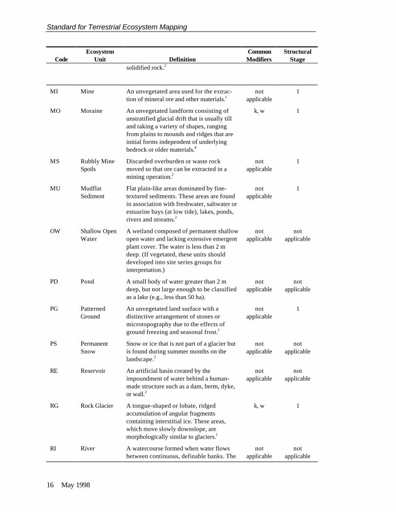
Units that occur in the landscape but are not defined site series, such as rock outcrops, cliffs,talus, urban/suburban areas, cultivated fields, and water bodies, are also mapped using a two-letter code. Standardized codes and definitions for these are listed in Table 3.1, as are sitemodifiers and structural stages. Some units, such as lakes (LA), will not have site modifiersor structural stages. If a site series code occurs that is the same as one of the codes below,the site series code takes precedence and a new code must be used for the non-vegetated,sparsely vegetated, or anthropogenic unit.
Table 3.1 Codes and definitions for non-vegetated, sparsely vegetated, andanthropogenic units
CodeEcosystem
Unit DefinitionCommonModifiers
StructuralStage
AL Alkaline Pond A body of fresh water with a pH greaterthan 7 and a depth less than 2 m.1
notapplicable
notapplicable
BA Barren Land devoid of vegetation due to extremeclimatic or edaphic conditions.1
k, r, w 1
BE Beach The area that expresses sorted sedimentsreworked in recent time by wave action. Itmay be formed at the edge of fresh or saltwater bodies.2
notapplicable
1
BF Blockfields,Blockslopes,Blockstreams
Level or gently sloping areas that arecovered with moderately sized or large,angular blocks of rock derived from theunderlying bedrock or drift by weatheringand/or frost heave, and that have notundergone any significant downslopemovement.1
k, r, w 1
CA Canal An artificial watercourse created fortransport, drainage, and/or irrigationpurposes.
notapplicable
notapplicable
CB Cutbank A part of a road corridor or river coursesituated upslope of the road or river, whichis created by excavation and/or erosion ofthe hillside.2
k, w 1

3.0 Mapping Conventions
May 1998 15
CodeEcosystem
Unit DefinitionCommonModifiers
StructuralStage
CF CultivatedField
A flat or gently rolling, non-forested, openarea that is subject to human agriculturalpractices (including plowing, fertilizationand non-native crop production) whichoften result in long-term soil andvegetation changes.
notapplicable
1, 2, 3
CL Cliff A steep, vertical or overhanging rock face.3 q, z 1
CO CultivatedOrchard
An agricultural area composed of single ormultiple tree species planted in rows.Pruning maintains low, bushy trees.
notapplicable
3
CV CultivatedVineyard
An agricultural area composed of single ormultiple species of grapes planted in rows,usually supported on wood or wiretrellises.
notapplicable
3
ES Exposed Soil Any area of exposed soil that is notincluded in any of the other definitions. Itincludes areas of recent disturbance, suchas mud slides, debris torrents, avalanches,and human-made disturbances (e.g.,pipeline rights-of-way) where vegetationcover is less than 5%.2
k, r, w 1
GB Gravel Bar An elongated landform generated bywaves and currents and usually runningparallel to the shore. It is composed ofunconsolidated small rounded cobbles,pebbles, stones, and sand.
notapplicable
1
GC Golf Course Flat to gently rolling grass-coveredthroughways and open areas set out forthe playing of golf. The fairways areusually separated by isolated rows orpatches of trees, shrubs and small bodiesof water (forested areas and water bodiesto be mapped as separate units).
notapplicable
2–7
GL Glacier A mass of perennial snow and ice withdefinite lateral limits. It typically flows in aparticular direction.2
notapplicable
notapplicable
GP Gravel Pit An area exposed through the removal ofsand and gravel.2
k,w 1
LA Lake A naturally occurring static body of water,greater than 2 m deep in some portion. Theboundary for the lake is the natural highwater mark.2
notapplicable
notapplicable
LB Lava Bed An area where molten rock has flowed froma volcano or fissure and cooled to form
k, r, w 1
Standard for Terrestrial Ecosystem Mapping
16 May 1998
CodeEcosystem
Unit DefinitionCommonModifiers
StructuralStage
solidified rock.2
MI Mine An unvegetated area used for the extrac-tion of mineral ore and other materials.1
notapplicable
1
MO Moraine An unvegetated landform consisting ofunstratified glacial drift that is usually tilland taking a variety of shapes, rangingfrom plains to mounds and ridges that areinitial forms independent of underlyingbedrock or older materials.4
k, w 1
MS Rubbly MineSpoils
Discarded overburden or waste rockmoved so that ore can be extracted in amining operation.2
notapplicable
1
MU MudflatSediment
Flat plain-like areas dominated by fine-textured sediments. These areas are foundin association with freshwater, saltwater orestuarine bays (at low tide), lakes, ponds,rivers and streams.2
notapplicable
1
OW Shallow OpenWater
A wetland composed of permanent shallowopen water and lacking extensive emergentplant cover. The water is less than 2 mdeep. (If vegetated, these units shoulddeveloped into site series groups forinterpretation.)
notapplicable
notapplicable
PD Pond A small body of water greater than 2 mdeep, but not large enough to be classifiedas a lake (e.g., less than 50 ha).
notapplicable
notapplicable
PG PatternedGround
An unvegetated land surface with adistinctive arrangement of stones ormicrotopography due to the effects ofground freezing and seasonal frost.1
notapplicable
1
PS PermanentSnow
Snow or ice that is not part of a glacier butis found during summer months on thelandscape.2
notapplicable
notapplicable
RE Reservoir An artificial basin created by theimpoundment of water behind a human-made structure such as a dam, berm, dyke,or wall.2
notapplicable
notapplicable
RG Rock Glacier A tongue-shaped or lobate, ridgedaccumulation of angular fragmentscontaining interstitial ice. These areas,which move slowly downslope, aremorphologically similar to glaciers.1
k, w 1
RI River A watercourse formed when water flowsbetween continuous, definable banks. The
notapplicable
notapplicable

3.0 Mapping Conventions
May 1998 17
CodeEcosystem
Unit DefinitionCommonModifiers
StructuralStage
flow may be intermittent or perennial. Anarea that has an ephemeral flow and nochannel with definable banks is notconsidered a river.2
RM ReclaimedMine
A mined area that has plant communitiescomposed of a mixture of agronomic ornative grasses, forbs, and shrubs.
k, r, w 1, 2, 3
RN RailwaySurface
A roadbed with fixed rails for possiblysingle or multiple rail lines.2
notapplicable
notapplicable
RO Rock Outcrop A gentle to steep, bedrock escarpment oroutcropping, with little soil developmentand sparse vegetative cover.
k, r, w 1
RP Road Surface An area cleared and compacted for thepurpose of transporting goods andservices by vehicles.2
notapplicable
notapplicable
RR Rural Any area in which residences and otherhuman developments are scattered andintermingled with forest, range, farm land,and native vegetation or cultivated crops.(Forested areas and cultivated fieldsshould be mapped as separate units.)1
notapplicable
notapplicable
RU Rubble Rubble is common on the ground surfacein and adjacent to alpine areas, onridgetops, gentle slopes and flat areas dueto the effects of frost heaving.2, 4
k, r, w 1
SW Saltwater Any body of water that contains salt or isconsidered to be salty.2
notapplicable
notapplicable
TA Talus Angular rock fragments of any sizeaccumulated at the foot of steep rockslopes as a result of successive rock falls.It is a type of colluvium.2, 4
k, r, w 1
TS Mine Tailings Solid waste materials directly produced inthe mining and milling of ore.2
notapplicable
1
UR Urban/Suburban
An area in which residences and otherhuman developments form an almostcontinuous covering of the landscape.These areas include cities and towns,subdivisions, commercial and industrialparks, and similar developments bothinside and outside city limits. (Forestedareas, such as parks, should be mapped asseparated units.)1
notapplicable
notapplicable
1 Dunster and Dunster (1996)2 Resources Inventory Committee (1997a)3 Sinnemann (1992)4 Howes and Kenk (1997)

Standard for Terrestrial Ecosystem Mapping
18 May 1998
3.2.2 Site modifiers
Each site series within the Ministry of Forests biogeoclimaticecosystem classification has been described by a “typical” set ofenvironmental conditions focusing specifically on important site,soils, and terrain characteristics (see Provincial Site SeriesMapping Codes and Typical Environmental Conditions TEMwebsite in Appendix B). The variation within some site series may be well described by thetypical conditions; for others, the typical conditions may describe only one possible set. InTEM, site modifiers (presented in Table 3.2) are used to describe these atypical conditions foreach ecosystem. Site modifiers provide additional descriptors for an ecosystem, and, ifapplicable, are displayed as the second component of an ecosystem unit.
If a site series occurs over a considerable range of site conditions in the landscape, sitemodifiers will be used for mapping the entire range of sites that do not meet the typicalsituation for that site series, within the limits of the modifiers described in Table 3.2. Forexample, the zonal site series for a particular biogeoclimatic unit usually occurs on gentleslopes with deep, medium-textured soils and mesic moisture regime. As an example, thesymbol LP would be used for the zonal FdPl–Pinegrass–Feathermoss site series in theIDFdk3 biogeoclimatic subzone. If this site series was found to occur on cool aspects withdeep soils, it would be mapped as LPk (Figure 3.6). If it also occurred on shallow soils of coolaspects, it would then be mapped as LPks. Up to two site modifiers can be used in defining anecosystem unit in the map labels. If more site modifiers are applicable, they can be added inthe database comments field. Site modifiers should be listed alphabetically in map symbols.
Table 3.2 Site modifiers for atypical conditions
Code Criteria
Topography
a active floodplain1 – the site series occurs on an active fluvial floodplain (level or very gentlysloping surface bordering a river that has been formed by river erosion and deposition),where evidence of active sedimentation and deposition is present.
g gullying1 occurring – the site series occurs within a gully, indicating a certain amount ofvariation from the typical, or the site series has gullying throughout the area beingdelineated.
h hummocky1 terrain (optional modifier) – the site series occurs on hummocky terrain,suggesting a certain amount of variability. Commonly, hummocky conditions are indicated bythe terrain surface expression but occasionally they occur in a situation not described byterrain features.
j gentle slope – the site series occurs on gently sloping topography (less than 25% in theinterior, less than 35% in the CWH, CDF, and MH zones).
k cool aspect – the site series occurs on cool, northerly or easterly aspects (285°–135°), onmoderately steep slopes (25%–100% slope in the interior and 35%–100% slope in the CWH,CDF and MH zones).
n fan1 – the site series occurs on a fluvial fan (most common), or on a colluvial fan or cone.
q very steep cool aspect – the site series occurs on very steep slopes (greater than 100%

3.0 Mapping Conventions
May 1998 19
Code Criteria
slope) with cool, northerly or easterly aspects (285°–135°).
r ridge1(optional modifier) – the site series occurs throughout an area of ridged terrain, or itoccurs on a ridge crest.
t terrace1 – the site series occurs on a fluvial or glaciofluvial terrace, lacustrine terrace, or rockcut terrace.
w warm aspect – the site series occurs on warm, southerly or westerly aspects (135°–285°), onmoderately steep slopes (25%–100% slope in the interior and 35%–100% slope in the CWH,CDF and MH zones).
z very steep warm aspect – the site series occurs on very steep slopes (greater than 100%) onwarm, southerly or westerly aspects (135°–285°).
Moisture
x drier than typical (optional modifier) – describes part of the range of conditions forcircummesic ecosystems with a wide range of soil moisture regimes or significantly differentsite conditions. For example, SBSmc2/01 (Sxw–Huckleberry) has three site phases described,and the submesic phase can be labeled with the “drier than average” modifier (e.g., SBx). Thiscode should be applied only after consultation with the Regional Ecologist.
y moister than typical (optional modifier) – describes part of the range of conditions forcircummesic ecosystems with a wide range of soil moisture regimes or significantly differentsite conditions. For example, SBSmk1/06 (Sb–Huckleberry–Spirea) is “typically” described assubmesic to mesic. When this site series is found on subhygric or hygric sites, the “y”modifier is used (e.g., BHy). This code should be applied only after consultation with theRegional Ecologist.
Soil
c coarse-textured soils 2 – the site series occurs on soils with a coarse texture, including sandand loamy sand; and also sandy loam, loam, and sandy clay loam with greater than 70%coarse fragment volume.
d deep soil – the site series occurs on soils greater than 100 cm to bedrock.
f fine-textured soils 2 – the site series occurs on soils with a fine texture including silt and siltloam with less than 20% coarse fragment volume; and clay, silty clay, silty clay loam, clayloam, sandy clay and heavy clay with with less than 35% coarse fragment volume.
m medium-textured soils – the site series occurs on soils with a medium texture, including sandyloam, loam and sandy clay loam with less than 70% coarse fragment volume; silt loam and siltwith more than 20% coarse fragment volume; and clay, silty clay, silty clay loam, clay loam,sandy clay and heavy clay with more than 35% coarse fragment volume.
p peaty material – the site series occurs on deep organics or a peaty surface (15–60 cm)3 overmineral materials (e.g., on organic materials of sedge, sphagnum, or decomposed wood).
s shallow soils – the site series occurs where soils are considered to be shallow to bedrock(20–100 cm).
v very shallow soils – the site series occurs where soils are considered to be very shallow tobedrock (less than 20 cm).
1 Howes and Kenk 19972 Soil textures have been grouped specifically for the purposes of ecosystem mapping.3 Canada Soils Survey Committee, 1987

Standard for Terrestrial Ecosystem Mapping
20 May 1998
Figure 3.6 Use of site modifiers in mapping site series
3.2.3 Vegetation developmental units
Structural stages
Structural stage numbers (Table 3.3) must be indicated foreach ecosystem unit (including non-forested units) except asnoted in Table 3.1. Additional substages are used to furtherdifferentiate structural stages 1 through 3 according to lifeform, layers and relative cover of individual strata. Substages 1a, 1b and 2a–d should be usedif photo interpretation is possible, otherwise, stage 1 and 2 should be used. Substages 3a, and3b should be used for permanent shrub communities (e.g., krummholz), and for detailedmapping projects where this differentiation is required for interpretations. Structural stagesand substages are described in Table 3.3.

3.0 Mapping Conventions
May 1998 21
Table 3.3 Structural stages and codes1
Structural Stage Description
Post-disturbance stages or environmentally induced structural development
1 Sparse/bryoid2 Initial stages of primary and secondary succession; bryophytes and lichensoften dominant, can be up to 100%; time since disturbance less than 20 yearsfor normal forest succession, may be prolonged (50–100+ years) where thereis little or no soil development (bedrock, boulder fields); total shrub and herbcover less than 20%; total tree layer cover less than 10%.
Substages
1a Sparse2 Less than 10% vegetation cover;
1b Bryoid2 Bryophyte- and lichen-dominated communities (greater than 1/2 of totalvegetation cover).
Stand initiation stages or environmentally induced structural development
2 Herb2 Early successional stage or herbaceous communities maintained byenvironmental conditions or disturbance (e.g., snow fields, avalanche tracks,wetlands, grasslands, flooding, intensive grazing, intense fire damage);dominated by herbs (forbs, graminoids, ferns); some invading or residualshrubs and trees may be present; tree layer cover less than 10%, shrub layercover less than or equal to 20% or less than 1/3 of total cover, herb-layercover greater than 20%, or greater than or equal to 1/3 of total cover; timesince disturbance less than 20 years for normal forest succession; manyherbaceous communities are perpetually maintained in this stage.
Substages
2a Forb-dominated2 Herbaceous communities dominated (greater than 1/2 of the total herb cover)by non-graminoid herbs, including ferns.
2b Graminoid-dominated2
Herbaceous communities dominated (greater than 1/2 of the total herb cover)by grasses, sedges, reeds, and rushes.
2c Aquatic2 Herbaceous communities dominated (greater than 1/2 of the total herb cover)by floating or submerged aquatic plants; does not include sedges growing inmarshes with standing water (which are classed as 2b).
2d Dwarf shrub2 Communities dominated (greater than 1/2 of the total herb cover) by dwarfwoody species such as Phyllodoce empetriformis, Cassiope mertensiana,Cassiope tetragona, Arctostaphylos arctica, Salix reticulata, andRhododendron lapponicum. (See list of dwarf shrubs assigned to the herblayer in the Field Manual for Describing Terrestrial Ecosystems) .
3 Shrub/Herb3 Early successional stage or shrub communities maintained by environmentalconditions or disturbance (e.g., snow fields, avalanche tracks, wetlands,grasslands, flooding, intensive grazing, intense fire damage); dominated byshrubby vegetation; seedlings and advance regeneration may be abundant;tree layer cover less than 10%, shrub layer cover greater than 20% or greaterthan or equal to 1/3 of total cover.

Standard for Terrestrial Ecosystem Mapping
22 May 1998
Structural Stage Description
Substages
3a Low shrub3 Communities dominated by shrub layer vegetation less than 2 m tall; may beperpetuated indefinitely by environmental conditions or repeateddisturbance; seedlings and advance regeneration may be abundant; timesince disturbance less than 20 years for normal forest succession.
3b Tall shrub3 Communities dominated by shrub layer vegetation that are 2–10 m tall; maybe perpetuated indefinitely by environmental conditions or repeateddisturbance; seedlings and advance regeneration may be abundant; timesince disturbance less than 40 years for normal forest succession.
Stem exclusion stages
4 Pole/Sapling4 Trees greater than 10 m tall, typically densely stocked, have overtoppedshrub and herb layers; younger stands are vigorous (usually greater than10–15 years old); older stagnated stands (up to 100 years old) are alsoincluded; self-thinning and vertical structure not yet evident in the canopy –this often occurs by age 30 in vigorous broadleaf stands, which are generallyyounger than coniferous stands at the same structural stage; time sincedisturbance is usually less than 40 years for normal forest succession; up to100+ years for dense (5000–15 000+ stems per hectare) stagnant stands.
5 Young Forest4 Self-thinning has become evident and the forest canopy has begundifferentiation into distinct layers (dominant, main canopy, and overtopped);vigorous growth and a more open stand than in the pole/sapling stage; timesince disturbance is generally 40–80 years but may begin as early as age 30,depending on tree species and ecological conditions.
Understory reinitiation stage
6 Mature Forest4 Trees established after the last disturbance have matured; a second cycle ofshade tolerant trees may have become established; understories become welldeveloped as the canopy opens up; time since disturbance is generally80–140 years for biogeoclimatic group A5 and 80–250 years for group B.6
Old-growth stage
7 Old Forest4 Old, structurally complex stands composed mainly of shade-tolerant andregenerating tree species, although older seral and long-lived trees from adisturbance such as fire may still dominate the upper canopy; snags andcoarse woody debris in all stages of decomposition typical, as are patchyunderstories; understories may include tree species uncommon in thecanopy, due to inherent limitations of these species under the givenconditions; time since disturbance generally greater than 140 years forbiogeoclimatic group A5 and greater than 250 years for group B.6
1 In the assessment of structural stage, structural features and age criteria should be considered together. Broadleaf stands will generallybe younger than coniferous stands belonging to the same structural stage.
2 Substages 1a, 1b and 2a–d should be used if photo interpretation is possible, otherwise, stage 1 and 2 should be used.3 Substages 3a and 3b may, for example, include very old krummholz less than 2 m tall and very old, low productivity stands (e.g.,
bog woodlands) less than 10 m tall, respectively. Stage 3, without additional substages, should be used for regenerating forestcommunities that are herb or shrub dominated, including shrub layers consisting of only 10–20% tree species, and undergoingnormal succession toward climax forest (e.g., recent cut-over areas or burned areas).
4 Structural stages 4–7 will typically be estimated from a combination of attributes based on forest inventory maps and aerialphotography. In addition to structural stage designation, actual age for forested units can be estimated and included as an attribute inthe database, if required.
5 Biogeoclimatic Group A includes BWBSdk, BWBSmw, BWBSwk, BWBSvk, ESSFdc, ESSFdk, ESSFdv, ESSFxc, ICHdk,ICHdw, ICHmk1, ICHmk2, ICHmw3, MS (all subzones), SBPS (all subzones), SBSdh, SBSdk, SBSdw, SBSmc, SBSmh,SBSmk, SBSmm, SBSmw, SBSwk1 (on plateau), and SBSwk3.
6 Biogeoclimatic Group B includes all other biogeoclimatic units (see Appendix C).

3.0 Mapping Conventions
May 1998 23
Structural stage modifiers (optional attribute) are used when required for furtherdifferentiation of structural stages 3 to 7. These modifiersdescribe five stand structure types based on the relativedevelopment of overstory, intermediate, and suppressed crownclasses (Table 3.4, Figure 3.7).
Table 3.4 Structural stage modifiers1 and codes2
Modifier Description
s single storied Closed forest stand dominated by the overstory crown class(dominant and co-dominant trees); intermediate and suppressedtrees account for less than 20% of all crown classes combined3;advance regeneration in the understory is generally sparse.
t two storied Closed forest stand co-dominated by distinct overstory andintermediate crown classes; the suppressed crown class is lackingor accounts for less than 20% of all crown classes combined3;advance regeneration is variable.
m multistoried Closed forest stand with all crown classes well represented; eachof the intermediate and suppressed classes account for greaterthan 20% of all crown classes combined3; advance regenerationis variable.
i irregular Forest stand with very open overstory and intermediate crownclasses (totaling less than 30% cover), and well-developedsuppressed crown class; advance regeneration is variable.
h shelterwood Forest stand with very open overstory (less than 20% cover) andwell-developed suppressed crown class and/or advanceregeneration in the understory; intermediate crown class isgenerally absent.
1 Adapted from Weetman et al. (1990). Stand structure types and crown classes are further described and illustrated inFigure 3.7.
2 Structural stage modifiers should be used as in the following examples: 5s for young forest stage with single-storiedstructure or 7m for old forest with multistoried structure. The only structural stage modifier, other than singlestoried, generally applicable to structural stage 3 is “h” (for shelterwood). This can be used to describe recentlyregenerated stands with a very open overstory (less than 20% cover of mature trees or vets) and a (usually dense)understory of seedlings and saplings.
3 Based on either basal area or percent cover estimates.

Standard for Terrestrial Ecosystem Mapping
24 May 1998
Figure 3.7 Structural stage modifiers
Stand composition modifiers (optional attribute) are usedas required for further differentiation of structural stages 3 to 7.These modifiers differentiate coniferous, broadleaf, and mixedstands (Table 3.5).
Table 3.5 Stand composition modifiers1, 2 and codes
Modifier Description
C coniferous Greater than 3/4 of total tree layer cover3 is coniferous
B broadleaf Greater than 3/4 of total tree layer cover3 is broadleaf
M mixed Neither coniferous or broadleaf account for greater than 3/4 of total treelayer cover3
1 Adapted from RIC, 1997a.2 Stand composition modifiers should be used as in the following examples: 6C for mature forest of coniferous
composition, 7mM for old forest with multistoried structure and mixed composition, 3bC for tall shrub communitydominated by coniferous saplings.
3 Stand composition modifiers emphasize overstory and intermediate tree layers, since these are the most visible onaerial photographs.

3.0 Mapping Conventions
May 1998 25
Seral community types1 (optional attribute)
Seral community types (Table 3.6) are an optional ecosystemattribute that should only be used in mapping where projectobjectives and survey intensity level warrant this level ofdetail. For instance, if seral floristic differences are relevant (as,for example , in the assessment of forage species or competingvegetation complexes) a floristic classification of seral community types may be required ina mapping project. A description of seral plant communities is useful for determining wherethe current plant community falls on the scale between early seral and potential naturalcommunity climax for any community type. (Province of BC, 1995b).
Given lack of data on seral ecosystems, there is not a current standard list of seral communitytypes for the province. Therefore, classification and mapping of seral community types mustbe approved by the Regional Ecologist during a mapping project. This will help to ensure somedegree of standardization and correlation of seral units as they are proposed. A list ofcurrently used seral community types and their codes is being maintained with the ProvincialSite Series Mapping Codes and Typical Environmental Conditions on the TEM website(see Appendix B). Seral community types are named using two or three typical or dominantspecies (e.g., trembling aspen–creamy peavine), and are given a two-letter lower-case code(e.g., ap).
Table 3.6 Example seral community types for the BWBSmw2
Seral Community Code Seral Community Name (DeLong, 1988)
ap At – creamy peavine
ak At – kinnikinnick
as At – soopolallie
al At – Labrador tea
ab At – black twinberry
ao At – oak fern
ac Ac – cow parsnip
3.2.4 Alternate methods for assigning site modifiers and structural stage
Site modifiers are usually estimated from air photographs. However, an alternative tointerpreting these attributes is to model them from existing digital data sources. For example,TRIM data can be used to determine aspect modifiers and terrain attributes could be used toassign certain other site modifiers. Modelling is acceptable if it provides results similar to airphoto interpretation.
1 We limit the term “seral” here to the developmental stages of an ecological succession not including the climax
community (Lincoln et al., 1982). We recognize that, in the ecological literature, climax communities are alsotechnically considered part of the sere.

Standard for Terrestrial Ecosystem Mapping
26 May 1998
Similarly, structural stage, structural stage modifiers, and stand composition modifiers areusually estimated from air photos. Alternatively, the forest cover database (specifically theage, species composition, and stocking criteria) is a useful source of information for assigningthese attributes. In fact, it should be possible, using this database in combination with somefield verification, to model structural stage for a given study area and assign structural stage toecosystem polygons using GIS programming algorithms . Modelling of a dynamic attributesuch as structural stage may better facilitate future updates from the forest cover mapping.However, modelling requires expertise and software that may not be readily available to allmapping contractors. Where modelling of structural stage is used, it may be preferable forinterpretations to keep it as a separate layer within the GIS.
3.2.5 Naming ecosystem units
Ecosystem units are named according to the site series name, site modifiers, and structuralstage. For example, the ICHvk/01: CwHw–Devil’s club–Lady fern unit, with the map codeRD, would be given the ecosystem unit name “CwHw–Devil’s club–Lady fern; typic.” Thesame site series on cool aspect sites and in mature forest (e.g., RDk6) would be named“CwHw–Devil’s club–Lady fern; cool aspect; mature forest.”
3.3 Ecosystem Map Units
Ecosystem map units are either simple, containing one ecosystem unit, or compound,containing up to three ecosystem units (for which one or all of the three attributes: site series,site modifier, and structural stage differ one from the other) (see Figure 3.8). The proportionof ecosystem units is indicated with “deciles.” Ecosystem map units may also have minorinclusions that are too small to map at the scale of the survey.
Figure 3.8 Compound map units
An ecosystem map unit should have a limited range of characteristics, so that it can beinterpreted and treated uniformly (e.g., it should not contain highly contrasting ecosystem unitsunless one is of minor extent and cannot be feasibly mapped as a separate simple unit). Theobjectives of the survey will often determine which characteristics are important.
Only ecosystem units that occupy 20% or more of a polygon are typically indicated in the maplabel. Those that occupy less than 20% of the polygon (e.g., a small wetland) can be indicatedin the map label if they are particularly significant for an interpretation. Another option is toindicate these ecosystem units in the database comments field or as an on-site symbol. The

3.0 Mapping Conventions
May 1998 27
intent of this guideline is to minimize compound map units and encourage delineation of newpolygons where there is considerable complexity.
The inclusion of three ecosystem units in a compound map unit should be done sparingly.Nevertheless, it is recognized that in some study areas with a complex distribution of eco-systems, ecosystem units are difficult to separate and compound map units cannot be avoided.
Minimum Polygon Size
A minimum polygon size of 0.5 cm2 (e.g., 0.7 × 0.7 cm ) is recommended. This polygon sizecorresponds to a land area of: 0.5 ha, at a scale of 1:10 000; 2.0 ha, at 1:20 000; and 12.5 ha,at 1:50 000.
3.4 Terrain and Soil Attributes
Conventions for displaying terrain and soil drainage symbology on air photographs and in theterrestrial ecosystem map database should follow Howes and Kenk (1997), RIC (1994), andthe Canada Soil Survey Committee (1978) listed in Appendix B. The proportion of terraincomponents is indicated with deciles.
3.5 Polygon Boundaries
Figure 3.9 provides the standardized polygon boundary line weights—or, alternatively, colourboundaries—that should be used for final presentation of ecosystem mapping.
Figure 3.9 Standardized polygon boundary line weights
3.6 Options for Ecoregion/Biogeoclimatic Map UnitSymbols
On a map, the ecosection unit symbol should generally be presented above the biogeoclimaticunit symbol, with both enclosed by a circle (see Figure 3.2). A new symbol should be placedon the map whenever one or both of the two units change. Although this is the standard,alternative methods may work in special circumstances based on the approval of the projectecologist.

Standard for Terrestrial Ecosystem Mapping
28 May 1998
3.7 Options for Ecosystem Map Unit Symbols
With the use of GIS and a colour plotter, there are many alternatives for displaying theecosystem unit components on a terrestrial ecosystem map. The standard is presented inFigure 3.9 above. The alternatives are generally dictated by the needs of the clients ofthe map.
For example, if forestry staff are familiar with the site series numbers presented in theMinistry of Forests regional guides, they can produce maps with the two-digit numbers ratherthan the two-character codes. However, not all map units are site series. In these cases,accepted site series could be given the two-digit code (e.g., 01 for the zonal ecosystem), whilenon-correlated, generalized, grouped, or other ecosystem units could keep their appropriatetwo-letter code. Since ecosystem units have both alphabetic and numeric codes, it issuggested that a separator be used to distinguish the components. This alternative couldappear as follows and for this example, the components are separated by a period:
Simple unit: 01.7 Describes one site series andstructural stage, with no site modifier
Compound unit: 4.01.7–3.03.sw.5–3.RO.w.1
Describes a combination of site seriesand other units

4.0 Polygon Data and Interpretations
May 1998 29
4.0 Polygon Data and Interpretations
The greatest value of ecosystem unit characterization and mapping is in providinginterpretations for a variety of disciplines (for examples, see Klinka, 1976; Lindeburgh andTrowbridge, 1985; Lea et al., 1990; Cichowski and Banner, 1993; and BC Ministry of Forestsregional field guides) (Figure 4.1). The importance of interpretive mapping lies in theopportunities it gives users to evaluate the landbase for its land use values and sensitivities.The Forest Practices Code requires a number of land based interpretations related tooperational and strategic level planning. Landscape unit planning, forest development planningand biodiversity requirements for maintaining forest ecosystem networks (including retentionof old growth, the temporal and spatial distribution of cutblocks, and rare and endangered plantcommunities) are all examples of interpretations that can be accommodated by TEM.
Figure 4.1 Examples of possible interpretations from ecosystem map
For each mapping project, a digital map with an associated polygon database must beproduced. Some examples of polygon attributes included in the database are polygonnumber, site series, structural stage, and genetic material. The number of individual dataattributes that could be recorded for each map polygon is very large, especially compared tothe information actually portrayed in a map unit label. The interpretative capabilities of anygiven map are based on the amount of data associated with each mapped polygon. Through

Standard for Terrestrial Ecosystem Mapping
30 May 1998
the use of GIS, ecosystem map units may be combined to form interpretative or treatmentunits, where they share similar characteristics with regard to a specific resource value ormanagement interpretation. As well, ecosystem maps can be readily combined with other datasources (such as bedrock geology maps and soils mapping) to allow further resourceinterpretations.
To ensure standardization of baseline ecological information, minimum data standards (corepolygon attributes) have been developed for those data attributes common to manyinterpretations (Table 4.1). Additional attributes may be required to make specificinterpretations for a particular project. Based on discussions with potential ecosystem mapusers, interpretations and corresponding data attributes have also been identified and groupedinto five broad subject areas: biodiversity management, terrain and soils management, forestmanagement, range management and wildlife management. Table 4.2 provides examples ofpossible interpretations under each of these areas. Terrain stability mapping is not aninterpretation from TEM mapping, but is a separate mapping procedure.
4.1 Core Polygon DataThe attributes listed in Table 4.1 must be recorded for each map polygon. These coreattributes constitute the minimum information that must be included when 1:50 000 and largerscale ecological inventories are conducted in the province.2 Core attributes are primarilyinterpreted attributes. Some, such as structural stage and a few site modifiers, can bemodeled or derived from other sources. Others, such as Project name and ecosystemmapper are applied universally to the data file rather than interpreted for each polygon.Attributes such as ecosection and biogeoclimatic map unit designations need only be recordedonce for each ecosystem map unit, while ecosystem and terrain attributes may be recorded upto three times for compound polygons.
4.2 Polygon Data for Additional InterpretationsEcosystem mapping projects often focus on specific topics such as wildlife habitat suitabilityor forest site productivity. Ecological interpretations for such projects may require informationabout attributes not on the core attribute list. For example, information about tree crownclosure , stand composition modifiers, and site disturbance may be required to rate habitatcapability and suitability for certain wildlife species. These attributes would therefore have tobe included in the database so that the ecosystem map could be interpreted adequately. Adifferent data set (including soil and humus form attributes) would be required to determineforest site sensitivity.
Additional attributes that may be useful to enhance specific interpretations are presented inTable 4.2. The attributes are listed below the column heading for each particular type ofinterpretation. For example, detailed interpretations for site productivity may require infor-mation about some, or all, of the additional attributes listed under that column heading. Wildlifesuitability and capability interpretive mapping will require a separate set of data attributes, andeach species may even require different attributes. In most cases, more than one management 2 A standardized coding format for core polygon data should follow “Standards for Digital Terrestrial Ecosystem
Mapping (TEM) Data Capture in British Columbia.”

4.0 Polygon Data and Interpretations
May 1998 31
interpretation will be required to meet a project’s objectives. Careful planning at the outset willensure that all necessary data attributes are collected to meet these requirements.
The lists presented in Table 4.2 provide guidelines only. An initial step in every mappingproject should be to determine the desired uses of an ecological map and the interpretationsrequired. Data attributes for specific projects should be worked out with the client and otherusers at the early project planning stages. Ecological mappers can choose to collect (inconjunction with the core polygon information) data for an entire subject area (e.g., forestmanagement), or only data associated with a specific interpretation (e.g., forest sitesensitivity). The data requirements should always be determined by the scope and objectivesof the project.
Table 4.2 shows only a sample of potential management interpretations. The attributesincluded are based on our existing knowledge and understanding of ecosystem complexities.Required data attributes may also vary by region, locality, or, in the case of wildlife, by theparticular species of interest. Other forestry interpretations not listed here might be pestsusceptibility or potential growth-limiting factors for individual tree species. As mentionedabove, selected wildlife species or species groups may also necessitate the collecting of dataattributes not listed (e.g., arboreal lichen abundance, a significant forage requirement forcaribou in certain areas). Other attributes and interpretations will undoubtedly be consideredas we increase our knowledge of biodiversity and ecosystem dynamics.
Table 4.1 Core polygon attributes required for terrestrial ecosystem mapping
Project- or Mapsheet-Specific Attributes – repeated for all polygons
Project nameEcosystem mapperTerrain mapperSurvey intensity level
Polygon-Specific Attributes – unique for each polygon
Record one of each of the following elements or classes per polygon:Mapsheet numberPolygon numberData sourceEcosection unitBiogeoclimatic unit (zone and subzone; variant and phase required if present)Geomorphological processes (when present)Soil drainages
Record up to three ecosystem and/or terrain units per polygon (see Figure 3.8):Ecosystem attributes• Decile• Site series• Site modifier(s)• Structural stageTerrain attributes• Decile• Terrain texture (optional but should be done where possible; record up to three for each component)• Surficial material (record one for each component; could include a surficial subtype)• Qualifiers (when present, record one for each component)• Surface expression (record up to three for each component)

Standard for Terrestrial Ecosystem Mapping
32 May 1998
Table 4.2 Possible Terrestrial Ecosystem Mapping interpretations and the associatedattributes
GE
NE
RA
LIZ
ED
INT
ER
PR
ET
AT
ION
SE
cosy
stem
Rep
rese
ntat
ion
Pla
nt C
omm
unity
Con
serv
atio
nE
cosy
stem
Rar
ityG
ap A
naly
sis
Land
scap
e pl
anni
ng (
FE
NS
)R
ipar
ian
& W
etla
nd M
anag
emen
t
Soi
l & S
ite S
ensi
tivity
Mun
icip
al S
ettle
men
t Pla
nnin
gG
enet
ic M
ater
ials
& D
epth
Sur
face
Ero
sion
Pot
entia
lF
lood
ing
& H
igh
Wat
erW
indt
hrow
Haz
ard
Rec
reat
ion
Site
Sen
sitiv
ityS
ite In
dex/
Pro
duct
ivity
Veg
etat
ion
Pot
entia
lV
eget
atio
n C
ompl
exS
ite P
repa
ratio
nTr
ee S
peci
es S
elec
tion
Exi
stin
g C
attle
Cap
acity
Crit
ical
Wild
life
Hab
itat
Wild
life
Cap
abili
tyW
ildlif
e S
uita
bilit
yId
entif
ied
Wild
life
For
age
Pot
entia
l
SUBJECT AREAS Biodiversity Terrain/Soils Forestry Range Wildlife OPTIONAL ATTRIBUTES
Anthropogenic Sites* ü ü ü ü ü ü
Area of Polygon ü ü ü ü ü ü ü ü ü ü
Bedrock Type* ü ü ü ü ü
Coarse Fragments >2mm ü ü ü ü ü ü ü ü
Coarse Woody Debris ü ü ü ü ü ü ü üComposition of Leading species by Layer ü ü ü ü ü ü ü ü
Depth of Forest Floor ü ü ü ü ü ü üDepth to Root Restricting Layer ü ü ü ü ü ü ü ü ü üDepth to Water Table ü ü ü ü ü ü ü ü ü ü
Ecosystem Condition ü ü ü üEcosystem Defensibility ü ü ü ü
Ecosystem Viability ü ü ü üElevation ü ü ü ü ü ü ü ü ü ü ü
Flooding Regime* ü ü ü ü ü ü ü ü ü ü ü ü ü üForage Species ü ü ü ü ü ü
Humus Form ü ü ü ü ü ü üHydrogeomorphology ü ü ü ü ü ü ü ü
Hydrologic Classification* ü ü üLand Cover Classification (VRI)* ü üMicrosites (Avalanche, Cliffs, Wetlands) ü ü ü ü ü ü ü ü ü üMoisture Regime ü ü ü ü ü ü ü
Nutrient Regime ü ü ü ü ü ü ü üPartial Cover Flag (3) ü ü ü ü ü ü ü ü ü ü ü ü ü
Plant Community ü ü ü ü ü ü ü ü ü ü ü ü ü ü ü üPolygon Adjacency ü ü ü ü ü ü ü
Seral Community Type ü ü ü ü ü ü ü üShrub Crown Closure ü ü ü ü ü ü
Site Disturbance ü ü ü ü ü ü ü ü ü ü ü ü ü ü
Slope ü ü ü ü ü ü
Slope (Meso) Position ü ü ü
Soil Bulk Density (1)(2) ü ü ü ü ü ü

5.0 Map Legends
May 1998 33
5.0 Map Legends
A map legend provides a summarized description of all map unit components and mapsymbols, together with other supporting information including survey objectives, surveyintensity, location, field sampling, other data sources, aerial photograph reference numbers,and map credits.
The recommended type of legend for terrestrial ecosystem maps has an open format andinvolves a list of ecosystem units and symbols that may be mapped as simple or compoundmap units. A large number of unique map units can potentially result from this open legendformat. Mitchell et al., (1989) present further details on open and closed legend formats.
As a minimum, the items described in Table 5.1 should be included in all ecosystem maplegends. Figure 5.1 presents an example. The specific layout and the amount of spaceallocated to each category may vary by project, and other categories may be added asrequired (e.g., interpretive information for ecosystem units). It is important to keep in mindthat the map legend should contain only summary information that is generally expanded in thereport (called an “expanded legend”) accompanying the map.
Most agencies have specific requirements as to what must be in the expanded legend.Generally, an expanded legend will contain descriptive information for each mappedecosystem. This includes the site series name, all related coding, a description of typicalenvironmental characteristics, and the features that characterize atypical site series asidentified by the site modifiers. The expanded legend will also describe the vegetation relatedto structural stages and any important associated features. Presentation of the information canbe in a variety of formats. Examples of expanded legends can be found on the TEM website(see Appendix B).
Table 5.1 Minimum data to be included on map legends
Item Minimum Requirements Comments
1. Title Include:• Study area name• Map sheet number/s (NTS, BCGS)• Map scale• Date
Example: Ecosystem Units ofthe Date Creek ResearchArea, Prince Rupert ForestRegion, portion of map sheet93M 009 (1:20 000), February1992
2. Introduction Include:• Objectives of the mapping project (including
interpretations to be supported by the map)• Study area• Mapping standards (include reference to this
document and survey intensity level)
Sampling followed SurveyIntensity Level 4 (RIC 1995).
3. Map LabelFormat
Provide example labels of ecosection,biogeoclimatic, and ecosystem units components,clearly indicated.

Standard for Terrestrial Ecosystem Mapping
34 May 1998
Item Minimum Requirements Comments
4. MapBoundaries
Provide examples of all line types used todelineate polygons (see section 3.5), includingstudy area boundary and sample plot locations.
5. EcoregionUnits
List all applicable ecosections or ecoregions andtheir codes.
6. Biogeo-climaticUnits
List all applicable biogeoclimatic units and theircodes.
7. Site Units Provide a description of site units, including siteseries names, two-letter codes and site seriesnumbers, typical situations and moisture regime,assumed site modifiers and mapped site modifiers.
Detailed descriptions of siteunits should be provided in aseparate report.
8. Site Modifiers List mapped site modifier and code. Only modifiers used in themapping project need to belisted.
9. StructuralStages andModifiers
List structural stages, structural stage modifiersand codes.
List and describe all structuralstages, including the agecriteria specific to eachbiogeoclimatic subzone(see Table 3.3.)
10. Data Sources Include lists of all data sources in the project:• aerial photos (year, scale, all photo numbers,
colour or black and white)• all previously available data and maps, such
as forest cover, satellite imagery, base maps,etc.
• percent polygons and/or ha per inspectionchecked
• number and type of samples
11. Credits Include:• names of all mappers and field personnel• name of project supervisor• names of correlators and reviewers• co-ordinating and funding agencies• GIS personnel
12. Citation Provide the citation as it should be referenced inother reports.

5.0 Map Legends
May 1998 35
TERRESTRIAL ECOSYSTEM MAPPING OF THE PURCELL WILDERNESS CONSERVANCYMap sheets 82K/038, 039, 040, 048, 049, 050
Scale 1:20 000 December 1998
Introduction
This project provides detailed ecosystem mapping of the southeast corner of the Purcell Wilderness Conservancy, located in southeast BritishColumbia, east of Kootenay Lake.
Wildlife capability and suitability mapping will be produced for grizzly bear, elk, and mountain goat. Recreation opportunity and sensitivitymapping will also be completed. Detailed ecosystem mapping will provide the frame-work for appropriate resource management for these, andother wildlife species occurring within the management zone.
Mapping was completed following the methods as outlined in Standard for Terrestrial Ecosystem Mapping in British Columbia (RIC, 1998).Fieldwork was completed in August of 1998 using survey intensity level 4.
Ecosection and Biogeoclimatic Units Label Ecosystem Unit Label
Map Boundaries
Ecosection Study area boundary
Biogeoclimatic Unit Plot location symbol u
Ecosystem Unit
Ecosections: Biogeoclimatic Units
AT Alpine Tundra ZoneEPR: Eastern Purcell Mountains ESSFdk Dry Cool Engelmann Spruce Subalpine Fir
ESSFdkp Dry Cool Engelmann Spruce Subalpine Fir Parkland
Site ModifiersCode Criteria Code Criteriac coarse-textured soils m medium-textured soilsd deep soils (> 100 cm to bedrock) p peaty materialf fine-textured soils s shallow soils (20-100 cm to bedrock)j gentle slope (slope <25%) v very shallow (< 20 cm to bedrock)k cool aspect (285°–135°, slope >25%) w warm aspect (135°–285°, slope >25%)
Structural Stage Stand CompositionCode Structural Stage Code Description1 Sparse/Bryoid C coniferous2 Herb B broadleaf2d Dwarf Shrub M mixed3 Shrub/Herb3a Low Shrub3b Tall Shrub Structural Stage Modifiers4 Pole/Sapling s single-storied5 Young Forest (generally 40–80 years but may begin as early as age t two-storied
30, depending on tree species and ecological conditions.) m multistoried6 Mature Forest (ESSFdk is Group A, 80-140 yrs). i irregular7 Old Forest (ESSFdk is Group A, >140 yrs). h shelterwood
Figure 5.1 Example of Map Legend

Standard for Terrestrial Ecosystem Mapping
36 May 1998
Ecosystem UnitsAT Alpine Tundra ZoneMap
CodeSite
Series #Site Series Name1 Assumed
ModifiersTypical Conditions Moisture
RegimeMapped
ModifiersAW 00 White mountain
avens–Snow willowj gentle to moderate
slopesmesic k, s, w
HP 00 Heather–Woollypussytoes
j gentle to moderateslopes
submesic c, s, w
SP 00 Black alpine sedge–Woolly pussytoes
j moderate slopes,receiving sites
subhygric k, w
ESSFdk Dry Cool Engelmann Spruce Subalpine FirMap
CodeSite
Series #Site Series Name1 Assumed
ModifiersTypical Conditions Moisture
RegimeMapped
ModifiersDM 02 Fd–Douglas maple–
Soopolallied, m, w significant slope, warm
aspect, deep med-textured soils
xeric –subxeric
s
FA 01 Bl–Azalea–Foamflower
d, j, m gentle slope, deep, med-textured soils
mesic c, f, k, s
FG 03 Bl–Azalea–Grouseberry
d, j, m gentle, deep, med-textured, non-calcareous soils
subxeric–mesic
c, k, v
FH 06 Bl–Azalea–Horsetail d, j, m gentle to level slope,receiving sites, deepmed-textured soils
subhygric–hygric
c, f
FM 05 Bl–Azalea–Step moss d, j, m gentle, lower slope,moisture receiving,med-textured soils
subhygric c, f, k
FS 04 Bl–Azalea–Soopolallie d, j, m gentle slope, deep, med-textured, calcareoussoils
submesic–mesic
c
WS 07 Willow–Sedge d, j, m mineral wetland, deepmed-textured soils
subhydric f, p
ESSFdkp Dry Cool Engelmann Spruce Subalpine Fir ParklandMap
CodeSite
Series #Site Series Name1 Assumed
ModifiersTypical Conditions Moisture
RegimeMapped
ModifiersFV 00 Subalpine-fir–Willow–
Sitka valeriansteep slopes, snowavalanched
mesic–subhygric
j, k, w
HP 00 Heather–Woollypussytoes
d, j, m gentle slopes, deep med-textured soils
submesic k, w
WC 00 Willow–Cinquefoil j gentle slopes, receivingsites
subhygric k, w
1 Includes unclassified ecosystem unitsData SourcesThis mapping project is based on 1:20 000 black and white stereo aerial photography from Geographic Data BC taken in June of 1994. Basemap is from Terrain Resource Inventory Mapping (TRIM) from Geographic Data BC Forest cover maps (1994) from the Ministry ofForests, Nelson Region. A total of 22% polygon inspection was achieved. 27 full plots 107 ground inspections and 400 visual checks werecompleted.
CreditsMapped by Jill Forest and Jack Moss of Moss Mapping Limited, Pemberton, BC. Field data collection: Jill Forest, Jack Moss, Tom Hawthorne,Roberta Wolfe. Project supervisor: Roberta Wolfe. GIS personnel: Cynthia Smith. Correlation and Edit by: D.R. Brown and R.K. Bark,Resources Inventory Branch, Ministry of Environment, Lands & Parks, Victoria, BC. Funding provided by Forest Renewal British Columbia(FRBC), the Ministry of Environment, Lands & Parks, Nelson Region, and SPRUCE TREES, Kootenay Division.
CitationForest, J. & J. Moss. 1998. Ecosystem Mapping of the Purcell Wilderness Conservancy. Prepared for BC Environment, Nelson Region, inpartnership with FRBC and SPRUCE TREES, Kootenay Div. 6, 1:20 000 Maps.
Figure 5.1 Example of Map Legend (cont.)

6.0 Mapping and Field Survey Procedures
May 1998 37
6.0 Mapping and Field SurveyProcedures
Outlined here are the major steps required to develop an ecosystem map, from the projectplanning stage to production of the final map (Figure 6.1). Clearly understanding and adheringto all of these steps is critical to ensure the final map and interpretative products meet theproject objectives, fulfill the needs of clients, and conform to provincial standards.
6.1 Project Planning
Project planning is the most important step in a mapping and inventory project. It sets thescene for the entire mapping project from defining objectives for the study and ensuring theinvolvement of all necessary individuals and clients, to determining what map andinterpretative products are needed and deciding how those will be achieved.
6.1.1 Defining objectives and developing a working plan
The following guidelines can help the mapper develop a work plan for a mapping project:
• Define the purpose and objectives of the project.
• Determine the products required by clients (e.g., maps, interpretations, reports, legends,database, summary statistics, etc.).
• Plot study area boundaries on an overview map.
• Determine the scale and survey intensity level to use.
• Develop sampling plan.
• Determine the attributes to be collected and mapped.
• Determine project personnel, budgets, and scheduling of fieldwork and productcompletion.
• Determine GIS/digital requirements.
• Follow provincial standards set out for data collection, classification, mapping andpresentation.
Objectives of a mapping project should be determined through co-ordination and consultationwith clients, regional and provincial co-ordinators, and the mapping team. The objectives of anecosystem mapping project need to be clearly defined and documented, to ensure theyaddress the specific needs of the clients and meet provincial mapping standards. Well-definedobjectives serve as benchmarks for contract managers and mapping personnel.
Once survey objectives are defined, a decision about scale of mapping and survey intensitymust be made. Both must ensure that a balance is achieved between the desired map product

Standard for Terrestrial Ecosystem Mapping
38 May 1998
and available budget. Section 6.3.1 provides some guidelines for determining appropriatesurvey intensity levels for ecosystem mapping.
Figure 6.1 Summary of mapping and field survey procedures

6.0 Mapping and Field Survey Procedures
May 1998 39
6.1.2 Compiling existing data
The following guidelines can help the mapper compile existing data for a study area:
• Determine what resource information and maps exist for the study area and adjacentareas, and assess their utility.
• Determine the appropriate base map to use (keeping in mind that TRIM is the preferredbase where available).
• Review available aerial photography and obtain photographs that provide the appropriatescale, coverage, and quality.
• Review ecosystem classification and data relevant to the study area, including itsecoregion and biogeoclimatic classification (using appropriate regional field guides).
• Contact the Ministry of Forests Regional Ecologist for assistance in understanding thedistinguishing characteristics between biogeoclimatic units and similar site series, and inunderstanding how well defined the ecosystem classification is for the study area.
After an area has been selected for ecosystem mapping, all relevant map and point sourcedata must be compiled. This should include information on vegetation ecology, climate, forestcover, Vegetation Resource Inventory (if available), bedrock and surficial geology, soils,hydrology, satellite imagery, topography, and other resource information required to serve theobjectives of the project. Appendix B outlines the common data sources available and wherethey may be obtained.
Aerial photographs, of the kind and scale specified in the work plan, must be obtained. It ispreferable to have photographs that are equal to, or larger than, the scale at which the finalmap will be presented. Data points should be transferred from previous ecological sampling tothe alternate (non-typed) aerial photographs. Adjacent mapping projects of similarmethodology and scale should be reviewed and, if appropriate, the borders matched betweenthe two study areas. Satellite imagery can provide additional overview information of thetypes of landscapes and general vegetation cover present in the study area.
6.1.3 Conducting field reconnaissance
A field reconnaissance is essential to begin establishing relationships between aerialphotograph features and ecosystem characteristics on the ground. Field reconnaissanceshould be carried out after all relevant information has been collated and aerial photos havebeen obtained. Field reconnaissance gives the mapper time to develop a preliminaryunderstanding of:
• ecosystem (site series) distribution and observable landscape features in the study area(e.g., microclimate effects, soils, bedrock geology, surficial geology, vegetation succession,disturbance history);
• biogeoclimatic and ecoregion relationships in the study area;
• relationships between aerial photograph features and ground features; and
• access and logistics for field sampling.

Standard for Terrestrial Ecosystem Mapping
40 May 1998
The reconnaissance is also an opportunity for obtaining information on ecological classificationand sampling requirements and planning the tentative location of sampling transects. Someaerial photo pre-typing is necessary before field reconnaissance (see section 6.2).
The project objectives and working plan may have to be adjusted depending on the complexityinitially observed. It is important that the entire mapping team take part in the initialreconnaissance so that members can correlate observations of ecological processes in thestudy area. Even in remote areas where access is difficult and costly, field reconnaissance isrecommended.
6.1.4 Developing the working legend
The following guidelines can help the mapper create a working legend:
• Develop an initial list of ecosystem units (site series, site modifiers, structural stages, etc.)present or expected in a study area, and identify their relationships to topographic andterrain features in the area.
• Complete landscape sketches, portraying ecosystem and landform relationships, to helpdevelop mapping concepts and ensure consistency in mapping.
• Initiate discussions with Regional Ecologists regarding existing ecological classificationand defining new units for study area.
Field reconnaissance and pre-typing provide the basis for development of the working legend.Once the field reconnaissance has been completed, a tentative legend can be established,linking ecosystem units to recognizable terrain, landscape, and biological characteristics.These include such terrain and landscape attributes as surficial material and surfaceexpression, soil drainage, soil depth, slope , aspect, and slope position, and such biologicalcharacteristics as overstory tree species and stand density. The working legend should list allecosystem units that are expected to occur in the study area, and should include codes andnames (Table 6.1).

6.0 Mapping and Field Survey Procedures
May 1998 41
Table 6.1 Example working legend for mapping ecosystem unitsECOSECTION BIOGEOCLIMATIC BIOTERRAIN ECOSYSTEM
UNIT Landscape Position Surficial Material Soil Depth/Texture/Drainage UNITSOB BGxh1 Level areas Floodplain CDSouthern Okanagan Very Dry Terrace Coarse-textured ANOkanogan Hot Bunchgrass SWcBasin PA
Medium-textured SWFine-textured SWf
Organic not definedModerate Slopes Moraine Average Moisture Fine-textured SWf
Medium-textured SWCoarse-textured SWc
Moist PRColluvium Deep SW
Shallow WSVery Shallow WSv
Glaciofluvial Coarse-textured SWcMedium-textured SW
Glaciofluvial Deep ANwShallow WSw
Colluvial Deep SWwSteep Southerly Slopes Shallow WSw
Moraine Shallow WSwDeep SWwShallow WSw
Steep Northerly Aspect Colluvial SWkSWckPWkPWck
Glaciofluvial ANkSWck
Moraine SWk
6.2 Pre-typing of Aerial Photographs
Production of an ecosystem map begins with the pre-typing of aerial photographs. Theprocedure, which should involve all members of a mapping team, is the first step in helping theteam understand the ecosystem/terrain/topography relationships within the study area. Somepre-typing should be completed before field reconnaissance, to clarify relationships betweenphoto and ground features (see sections 6.1.3 and 6.1.4). The remaining aerial photos shouldbe typed before field sampling begins. Where mapping that follows the same standards andscale has been previously completed on adjacent areas, the aerial photos from that projectshould be obtained and border-matched with the new typing.
6.2.1 Conducting initial ecoregion/biogeoclimatic mapping
Existing ecoregion and biogeoclimatic maps and reports should be consulted during the pre-typing stage, and the latest biogeoclimatic line work should be redrawn at the project mapscale, using elevational models and obvious east–west or north–south boundaries. RegionalEcologists should be consulted to ensure that up-to-date information is being used. Because itis often very difficult to accurately delineate ecoregion and biogeoclimatic unit boundaries onaerial photos, the final mapping of most of these boundaries is usually done after field work iscomplete.
At the pre-typing stage, Alpine Tundra and subalpine parkland boundaries and approximateboundaries for the other biogeoclimatic units are mapped on aerial photos. The Alpine Tundraand subalpine parkland lines should be drawn before ecosystem map units are delineated. Thisprovides an initial boundary from which the other ecosystem map units can then be drawn.Other biogeoclimatic map unit boundaries can be drawn either on the typed or non-typed

Standard for Terrestrial Ecosystem Mapping
42 May 1998
photos, using a different colour than the ecosystem map units. These boundaries will need tobe confirmed in the field and finalized after fieldwork.
Delineating Alpine Tundra zone
By definition, the Alpine Tundra zone has alpine vegetation on zonal sites. The Alpine Tundrazone boundary is usually the upper elevation of discontinuous forest (parkland, includingkrummholz) or in the case of the Spruce–Willow–Birch (SWB) zone, the upper elevationallimit of extensive deciduous scrub (which is considered to be subalpine vegetation). The alpineboundary will have to be generalized at a consistent elevation (varying with aspect), becausecliffs , rock outcrops, and avalanche chutes often dissect the alpine/subalpine transition (e.g.,shrubby avalanche chutes are common in wetter subalpine forested subzones). Trees inkrummholz form (prostrate or low in stature) may occur in the alpine zone, but they are ofvery low cover. Some larger krummholz patches may occur in sheltered, non-zonal sites. Theplacement of the Alpine Tundra zone boundary is shown in Figure 6.2. Glaciers areconsidered to be in the biogeoclimatic zone that is expected at that elevation (e.g., glaciersoften extend into the subalpine and lower elevations).
Figure 6.2 Delineation of Alpine Tundra and parkland subzone
Delineating subalpine parkland
Where possible, parkland subzones of the Mountain Hemlock and Engelmann Spruce–Subalpine Fir and scrub subzones of the Spruce–Willow–Birch zones should be mapped. Theyare recognized as a distinct elevational transition from closed or continuous forest to thetreeless Alpine Tundra. Parkland is characterized by forest clumps interspersed with opensubalpine meadows, shrub thickets, and krummholz (Figure 6.2). However, parkland varies inthe proportion of treed patches versus open vegetation. It is often discontinuous andintermixed with rock outcrops, cliffs, or talus. Recognition of a distinct parkland subzone ismost obvious in gently rising plateau areas or rounded mountains of relatively gentle relief(e.g., the Quesnel Highlands). As with alpine, the parkland boundary will have to begeneralized at a consistent elevation.
In some areas, especially steep-sided coastal valleys, it is difficult to map subalpine parklandsubzones as continuous elevational bands. Parkland in these areas is very narrow and

6.0 Mapping and Field Survey Procedures
May 1998 43
discontinuous, and often dominated by sparsely vegetated ecosystems. In these cases, theentire subalpine subzone would be mapped as forested. Parkland-like ecosystems could thenbe delineated within the forested subzone as ecosystem units. For example, the biogeoclimaticunit could be designated as MHmm1 (implying that it is a forested unit), but much of the areamapped is sparsely vegetated rock, cliffs, and talus interspersed with patches of forest andheath. In such areas, tree growth is limited more by substrate (steep terrain and lack of soil)than by climate.
Even where a parkland subzone is mapped, parkland-like ecosystems may also occur in theforested subzone below, in areas (such as cirque basins) that receive cold air drainage, or inareas that have long snow duration and wet soils. These non-forested meadow and shrubcommunities, interspersed with forest patches, should be mapped as parkland-like ecosystemunits within the forested subzone; the parkland subzone boundary should not be brought downin elevation to include these ecosystems.
6.2.2 Conducting initial ecosystem mapping
Terrestrial ecosystem mapping integrates vegetation, terrain (surficial geology), and soilfeatures, both in terms of delineation criteria and database attributes. This “bioterrain”approach results in map units that portray ecosystem units (site series, site modifiers andstructural stages) with their associated terrain attributes (genetic material, surface expression,qualifiers , geomorphological process, soil drainage).
The interpretative value that results from this bioterrain approach to ecosystem mapping isgreatly increased over that of a pure vegetation, soils or terrain map. Since many terrain andlandscape features correlate well with ecosystem properties, ecosystem polygons aredelineated on aerial photos using a combination of recognizable permanent terrain andlandscape features, biological characteristics, and inferences related to significant changes inthe landscape (Figure 6.3). Refer to Table 6.2 for further explanation of delineation criteria.The resulting ecosystem map units can be developed in various ways, depending on theexperience of the mappers, but polygon delineation is most effectively carried out using aninterdisciplinary approach.
In order to develop a common understanding of ecosystem/terrain/landscape relationships, it isessential that the mapping team, usually composed of a vegetation ecologist and terrain/soilspecialist, work together on representative photographs. Delineation can then be carried outby either specialist, in a consistent manner, as long as feedback occurs throughout the rest ofthe pre-typing process.
A useful approach to the initial pre-typing of photographs is to mentally divide the study areainto broad landscape areas that have similar, repeatable map units and relationships(Figure 6.4). These areas can be determined from the working legend and consideration ofecosystem/site relationships in broad landscapes such as alpine, mountain slopes, valley floors,plateaus and plains. This frames the mapping process before more detailed terrain andvegetation features are considered.

Standard for Terrestrial Ecosystem Mapping
44 May 1998
Figure 6.3 Integrated delineation criteria for developing Ecosystem Map Unit polygons.
Table 6.2 outlines the main criteria that should be used to delineate ecological polygons andassign core ecosystem and terrain attributes for ecosystem map units. Note that individualpolygon attributes (e.g., site series, structural stage) are interpreted from one to many physicalor biological criteria (e.g., slope position, vegetation composition and structure) that are eitherdirectly observable on the photo (e.g., slope position) or inferred from visual photo features orcharacteristics (e.g., vegetation composition and structure are inferred from tone, texture,colour, shape, pattern). The assessment of any one attribute is thus an integrated process,whereby many criteria are being observed and processed simultaneously in order to predictthe attribute. Depending on the survey intensity level, a portion of the polygons will eventuallyhave their attributes confirmed through ground sampling.
An attempt should be made to consider all of the criteria from Table 6.2. As mappers gaingreater experience, this will become second nature. Other useful aids to aerial photointerpretation are the Vegetation Resources Inventory Photo Interpretation ProceduresManual (RIC 1997c), Howes and Kenk (1997), and Keser (1982).
Photo criteria can be integrated in many different ways, depending on the experience andbackground of the mapper. Some ecosystem or terrain boundaries, such as the edge of afloodplain or terrace, may be sharp (or “hard”) and clearly defined; other boundaries may begradational (or “soft”). The latter can be determined by combining attributes of theecosystems themselves with presumed terrain unit boundary features. The question ofwhether to lump or split polygons (e.g., to add or omit a boundary) is largely a matter ofjudgment, scale of mapping, and project objectives. Thus, if two or more experienced mappers

6.0 Mapping and Field Survey Procedures
May 1998 45
were to independently map the same area, some boundary positions would correspond exactly,some would be fairly similar, and some would differ markedly. For example , a mature,coniferous forest on an active floodplain in the SBS biogeoclimatic zone, representing aSpruce–Horsetail site series, would be delineated in likely the same way by different mappers.However, the extent of the same site series occurring on subdued morainal terrain in the SBSmight only be detected through a mapper recognizing subtle differences in speciescomposition, crown closure, stand age, structure, and landscape characteristics.Interpretations of these criteria would vary among mappers as would polygon delineations.
The mapping team must work out how it will approach these less well-defined areas, toensure a consistent approach to mapping is used. Where possible, the mappers should firstdelineate the hard terrain boundaries (these, in most cases, will coincide with ecosystemboundaries). Soft terrain boundaries can then be located either where there are subtlechanges in the physical conditions that influence ecosystems (such as surface expression, soildrainage, and geomorphological processes) or where there is a vegetation change suggesting achange in ecosystem unit.
During the pre-typing phase, mappers should label map units with initial terrain and soildrainage symbols (using deciles) following Howes and Kenk (1997). They should alsoindicate ecosystem attributes (e.g., one to three ecosystem units) for a considerable portion ofthe project area. However, if they are limited by time or a lack of familiarity with theecosystems in the map area, some mappers may only pre-type polygons with terrain labels.When this approach is taken, it is recommended that some attempt to label ecosystem mapunits for a portion of the study area be completed before field sampling, so that relationships ofecosystems to terrain attributes can be assessed in the field. The preferred system is to startwith field reconnaissance so that initial ecosystem map units can be assigned to most polygonsat the pre-typing stage.
Figure 6.4 A landscape profile for the ESSFwk1.

Standard for Terrestrial Ecosystem Mapping
46 May 1998
Table 6.2 Criteria for delineating ecosystem map units on aerial photographs1
CriteriaObservable Feature/Photo Characteristic
Applicable Mapped Attribute
Vegetation
Tree species composition Tone, texture, colour, size, shape,shadow
Site series2, structural stage(seral community type)
Understory or non-forestedvegetation composition orcharacteristics
Tone, texture, colour, Site series, structural stage(seral community type)
Canopy characteristics(including crown closure)
Tone, texture, colour, shape,shadow, size, pattern (open,closed, layered, clumpy)
Site series, structural stage(seral community type)
Height of stand (relativeproductivity)
Texture, size, pattern, tone,density
Site series, structural stage(seral community type)
Topography
Landscape position and shape Shape and three dimensionalcharacteristics
Site series, site modifier, soildrainage
Aspect Shape, three dimensionalcharacteristics and direction
Site series, site modifier
Slope Shape and three dimensionalcharacteristics
Site series, site modifier, soildrainage
Drainage pattern Shape, pattern and threedimensional characteristics
Site series, site modifier, soildrainage
Terrain
Landform/parent materialincluding surface expression,qualifiers, terrain texture (e.g.,active processes)
Topographic position,observable drainage and terrainpatterns, shape, topography,tone, colour (disturbance)
Inferred terrain texture, geneticmaterial, surface expression,qualifiers, site series, sitemodifier, soil drainage
Geomorphological process Patterns Geomorphological process, siteseries, site modifier
Soils
Soil drainage Tone, drainage patterns,topography
Soil drainage, site series, sitemodifier
Soil depth Colour, tone, texture, topography Soil drainage, site series, sitemodifier
Gradients/Patterns
Relationship to other map units Pattern, juxtaposition, sizeand edges
Various
Adjacent map units Pattern, juxtaposition, shapeand edges
Various
Polygon shape and orientation Pattern, juxtaposition, shape,edges and direction
Various
1 Refer to Vegetation Resources Inventory Photo Interpretation Procedures Manual (RIC, 1997c) for moreinformation on interpreting physical and biological attributes from aerial photographs.
2 Criteria used for site series assessment are by default also used for assessment of soil moisture and nutrient regimes,but these are not core attributes.

6.0 Mapping and Field Survey Procedures
May 1998 47
During pre-typing, structural stages may be interpreted from aerial photographs or taken fromother sources such as forest cover (or Vegetation Resource Inventory) maps, or a combinationof these two methods. The best approach should be determined by the date that the aerialphotographs were taken and by whether major disturbances have occurred since then.
The mapper should use judgment in delineating small polygons and should limit the complexityof polygon symbols, so that the mapping on the photos remains neat and legible. Photointerpretation is a skill that improves only with much practice, particularly in combination withground truthing to calibrate the eyes. The mapper needs to develop a mental model of how allthe pieces of information relate to the ecosystems that actually occur on the ground (Figure6.3). This model will have to be “recalibrated” for each new study area, as well as for eachbiogeoclimatic unit within a study area. These relationships are developed throughout allstages of the project, from initial reconnaissance, and pre-typing, through field sampling and onto final typing and labelling.
6.3 Field Sampling
Sampling is required to confirm ecosystem and terrain map unit designations and boundaries,to collect data for ecosystem descriptions in reports, and to develop or refine the classificationof ecosystem units. Sample types can be of varying detail, depending on their purpose. Theintensity of sampling should be related to project objectives and funding. Sample transects andplots provide site-specific information on the distribution and characteristics of plantcommunities, landforms/parent materials, soils, and on the interrelationships among theseecosystem components. This information can then be used to interpret ecosystemrelationships in the areas or polygons not sampled.
Determining sample intensity, sample detail, and location of transects and sample points isdiscussed in this section.
6.3.1 Establishing survey intensity
Survey intensity is a measure of sampling density and can be characterized either as thepercentage of polygons that have been field inspected, or as the actual density of fieldinspections on an area basis (hectares per field inspection). Table 6.3 defines six surveyintensity levels for ecosystem mapping and some of the factors to consider when planning amapping project. Table 6.4 translates each of the survey intensity/map scale combinations intoactual field inspection densities (hectares per field inspection). The table can be used toestimate how many field inspections would be required for study areas of various sizes, tomeet each of the survey intensity level requirements. Basing field sampling requirements onminimum density values rather than polygon inspection percentages is recommended, becausethe total number of polygons is usually not known until after field sampling.

Table 6.3 Survey intensity levels for ecosystem mapping
SurveyIntensity
Level
Percentageof PolygonInspections
Ratio ofFull Plots:
Ground Insp.:Visual Checks1
SuggestedScales
(K =1000)
AreaCovered by
0.5 cm2Range of Study Area
(ha) Interpretation Examples
1 76–100% 2 : 15 : 83 1:5 K to 1:10 K 0.25–0.5 ha 20–500 Site specific silviculture prescription; soilsensitivity to erosion, soil compaction, etc.
2 51–75% 3 : 17 : 80 1:10 K to 1:20 K 0.5–2 ha 100–10 000 Silviculture planning; tree species selection.
3 26–50% 5 : 20 : 75 1:10 K to 1:50 K 0.5–12.5 ha 5 000–50 000 Vegetation potential; forest productivity;habitat enhancement prescriptions.
42 15 – 25% 5 : 20 : 75 1:20 K to 1:50 K 2–12.5 ha 10 000–500 000 Forestry, wildlife capability; ecosystemrepresentation; general forest productivity;local resource planning; landscapemanagement planning.
53 5–14% 5 : 20 : 75 1:20 K to 1:50 K 2–12.5 ha 10 000–1 000 000 Forestry, wildlife capability; ecosystemrepresentation; general forest productivity;local resource planning; landscapemanagement planning.
R3,4 0–4% 0 : 25 : 75 1:20 K to 1:50 K 12.5–306 ha 50 000–1 000 000 + Regional planning; broad landscapemanagement planning.
1 Inspection ratios are guidelines; actual project ratio should be set by project ecologists responsible for administering project.2 Survey intensity level recommended for most mapping. This provides a reasonable balance of cost and reliability.3 Survey intensity level recommended when Level 4 is too costly and lower reliability is acceptable.4 Level R (reconnaissance) ecosystem mapping should only be conducted by ecologists who have considerable field experience in the ecosystems of the study area.

6.0 Mapping and Field Survey Procedures
May 1998 49
Table 6.4 Field inspection density for selected survey intensity/map scalecombinations
Hectares per inspection
Survey
intensity level1
1:5000
(940 ha/sheet)
1:10 000
(3800 ha/sheet)
1:20 000
(15 100 ha/sheet)
1:50 000
(60 400 ha/sheet2)
1 0.9–1.2 3.8–5 15–19 91–120
2 1.3–1.8 5.1–9 20–29 121–178
3 1.9–3.7 8–14 30–59 182–350
4 3.8–6.3 15–25 60–100 364–607
5 6.4–19 26–76 101–302 650–1820
R 18–94+ 77–370+ 303–1500+ 2275–9100+1 Values are guidelines only and are based on an average polygon size of 3–4 cm2. Mapsheet areas and hectares per
field inspection are based on an average map size; actual values will vary somewhat, depending on latitude.2 Based on new 1:50 000 mapsheets (blocks of four 1:20 000 maps)
The survey intensity used in the preparation of an ecosystem map should be determined byproject objectives and the proposed use of the map. If the map is to be used for makingspecific management decisions about portions of land (e.g., soil sensitivity to harvestingequipment, site preparation options, tree species selection), then the map needs to bevery reliable. Increased reliability is usually achieved through a higher survey intensity andselection of a larger map scale. However, both of these factors increase the cost of themapping project. If the map is to be used only for general land planning, then a lower surveyintensity is appropriate and mapping can be done at a smaller scale. A low survey intensitydoes not necessarily mean that a map will be less reliable, although this is generally the case.Other factors influencing reliability are ecosystem complexity, relationship of ecologicalvariation to readily identifiable aerial photo attributes, and surveyor knowledge and experience.
For example, in balancing cost and reliability of ecosystem mapping for landscape planningand wildlife capability/suitability, it is recommended that most mapping be conducted at level4. The appropriate scale would be 1:20 000 or 1:50 000, depending on the complexity ofecosystems and the requirement for accuracy. At 1:20 000, this translates into a minimum ofone inspection per 100 ha. If a lower cost and reliability is acceptable to the user, ecosystemmapping at level 5 or level R could be conducted.
Survey intensity level is not always related to scale; any intensity level can be conducted atany scale. However, smaller scale maps are generally used for land management planningand the higher costs of a more intense survey level are not usually warranted for broadmanagement planning. Table 6.3 includes scale as a guide only to determine intensity level.
Another consideration in selecting mapping scale is the scale of the aerial photographs andother imagery to be used. The final map scale should not be significantly larger than the photoscale, as it will be difficult (maybe even impossible) to recognize and delineate smallecosystems on the photos that should be delineated at the map scale.

Standard for Terrestrial Ecosystem Mapping
50 May 1998
6.3.2 Designing a sampling plan
A sampling plan is critical for focusing field work during brief sampling periods, and helpsensure that sampling occurs where it should. Field work is costly but important. Well-plannedfield sampling is more cost-effective and productive and results in more reliable map products.
In preparing a sampling plan, the mapper should consider the following elements for the studyarea:
• Size of study area
• Topography
• Previous ecological sampling (number, type, and location)
• Existing information (e.g., biogeoclimatic units, site series classification, adjacent ecosystemmapping, geology, terrain, and soils)
• Additional data collection requirements for samples (e.g., wildlife, coarse woody debris,mensuration, range) and polygon database attributes
• Interpretations to be produced from the mapping
• Survey intensity level
• Sampling ratio of full plots, ground inspections, and visual checks
• Possibility for “new” site units
• Access (using topographic, forest recreation, forest cover, and forest development maps,recent aerial photos, latest access information from Ministry of Forests District Office)
• Questions from pre-typing or development of working legend
• Knowledge level and experience of field crews and mappers in the ecosystems of the area.
The sampling plan needs to integrate this known information to design field transects anddemarcate potential sample plot locations. This will ensure that the project objectives are met,plots and inspections are well distributed and focused on objectives, and enough informationwill be compiled to finalize the pre-typing of the aerial photos.
A useful procedure to developing a sampling plan is to assess how all the above elementsmight affect the number and location of plots and inspections, and then start compiling theinformation on a set of maps at a smaller scale than the final mapping is to be (e.g., 1:50 000or 1:100 000). All known information that can be displayed at the map scale should bemapped (e.g., ecosection boundaries, biogeoclimatic subzone/variant boundaries, roads,helicopter access points, bedrock geology, areas of “uncommon” structural stages or siteconditions, existing plots). From this summary and evaluation, development of the samplingplan can begin.
Various sampling designs are possible for confirming and refining the pre-typing of polygons(see Forbes et al., 1982; Gillison and Brewer, 1985; Valentine, 1986; Mitchell et al., 1989).However, the most commonly used method of sampling in ecosystem mapping projects is theestablishment of field inspections along transects. The transects can be randomly located, butare more often selected to cover the greatest number and variety of polygons in the leastamount of field time. Sample points can be established systematically, at set distances along atransect, but are generally established subjectively.

6.0 Mapping and Field Survey Procedures
May 1998 51
Clear objectives for all field inspections should be articulated in the sampling plan. Someinspections may be to sample homogeneous areas for descriptive purposes, others to assesspolygon boundaries, or assess ecosystem unit proportions within polygons. Because of theircost, detailed plots and ground inspections should focus on uniform sites within polygons andavoid transitional areas. Sampling at slope, moisture, or soil boundaries makes it very difficultto ascertain ecological determining factors, unless numerous plots are establishedsystematically across the gradient. Visual checks can be planned to assess boundaries,confirm questionable areas from photo interpretation, or do whatever is necessary to confirmecosystem designations and to meet project objectives. Again, it is best to have some focusfor all plot inspections so that field crews are clear about their sampling objectives.
Sampling is required to characterize common and widespread ecosystem units, as well asthose units that occur infrequently, such as wetlands and riparian ecosystems . Samplingintensity may consider the relative confidence in local biogeoclimatic mapping or focus on siteseries that are difficult to identify at the pre-typing phase. Intensive sampling may be done inecosystems that are considered more valuable or more sensitive than others. For example, in arange mapping project, more sampling may have to be done in productive grasslandcommunities and in forests with open canopies and higher forage values. Similarly, for wildlifestudies, areas that are known winter ranges or are important for biological diversity (such asriparian ecosystems) may require more intensive sampling.
Using the set of maps with the compilation of resource information, and with the objectives ofeach of the sample types clearly articulated, the mapper should then plan where the transectswill be located. It is important to keep in mind that the sampling plan is only a plan—improvisation in the field will be required, as some transects may not sample as planned oraccess may be restricted (e.g., by road washouts, bad weather). Therefore, more transectsthan required should be planned. Flexibility is the key. A tally sheet should be designed tokeep track of what is sampled and what is still needed, and all information should becommunicated to crews to ensure they know what is required.
After the sampling plan is developed, it should be reviewed by the Regional Ecologist orproject ecologist to confirm that it meets the project objectives. The information(e.g., transects, required inspections) should then be transferred to the non-typed set of fieldphotos to make it easier to use in the field. A well-thought-out sampling design will greatlyincrease field efficiency.
6.3.3 Conducting field inspections and plot sampling
Field inspections are of three types: full plot, ground inspection, and visual check. Togetherthey are usually carried out in a 5:20:75 proportion, respectively (see Table 6.3). Full plots andground inspections are done at specific locations (point samples), guided by the sample plan.Ground inspections are less detailed than full plots and visual checks are less detailed thanground inspections. Visual checks may be completed either at specific sampling points or fora boundary or an entire polygon.

Standard for Terrestrial Ecosystem Mapping
52 May 1998
Full plots
Full plots, recorded on the Ecosystem Field Form (FS882 [1-7]), provide the most detailedecological data for a point sample and are intended for classification of site series,confirmation or classification of biogeoclimatic units, and development of ecosystem unitdescriptions and summary statistics. Whether samples are selective or designedsystematically along a transect, the boundaries of the actual sample plot should encompass ahomogeneous ecosystem in terms of soil and vegetation properties. This ensures that thedescriptive parameters and statistics recorded for individual ecosystems will be meaningful,and the characteristics of ecosystem units synthesized from the data accurate (Daubenmire,1968; Mueller-Dombois and Ellenberg, 1974).
A plot is a point sample and can only be considered representative of an entire polygon if thatpolygon is very uniform and of one ecosystem. In large or heterogeneous polygons, wheretwo or more ecosystem units occur, the surveyor could sample one ecosystem in detail andthen do ground inspections or visual checks in the others. Plot size should usually be 400 m2
in forested communities, but smaller plot sizes (100 m2) may be appropriate in uniform,species-poor, non-forested habitats such as occurs in some wetlands, grasslands, or alpineareas. Plots may be circular (11.3 m radius), square (20 × 20 m), or rectangular (e.g., 10 × 40m). Circular plots are generally easier to lay out using a plot radius cord and flagging a fewtrees to mark the circumference. However, a plot with dense understory of tall shrubs ortrees can impede vision and may be easier to mark in a rectangular shape. Plot shape mayvary to ensure that the plot encompasses a homogeneous unit.
Data collection procedures for full plots should follow the Field Manual for DescribingTerrestrial Ecosystems (BC Ministry of Forests and BC Ministry of Environment, 1998a).That guide updates some sections of Luttmerding et al. (1990) and is in a field guide format.Data describing the site, soil, vegetation, and mensuration or other required fields must berecorded on the Ecosystem Field Forms (FS882). Minimum data requirements for ecosystemmapping projects are shown in Table 6.5. For some projects, additional fields will have to becompleted to acquire the necessary data for interpretations.
As full plots account for only a small proportion of the inspections and are the most costly toestablish, they need to be carefully selected. The sampling plan should clearly set criteria forestablishment of these plots (e.g., one sample of each site series, two in each zonal site seriesto confirm biogeoclimatic units, three or more in a new site series).

6.0 Mapping and Field Survey Procedures
May 1998 53
Table 6.5 Minimum data collection requirements for Ecosystem Field Forms (FS882)
Site Form
1. Date (Y/D/M)2. Plot number3. Project Identification4. Surveyor(s)5. General location (should be specific enough
to find plot again easily)6. Forest region7. Mapsheet8. UTM (zone, easting and northing) or
latitude and longitude9. Air photo no. (incl. Flight line)10. Co-ordinates (X and Y)11. Site diagram12. Plot representing13. Biogeoclimatic unit14. Site series
15. Ecosection16. Moisture regime17. Nutrient regime18. Successional status19. Structural stage20. Realm/class (for wetlands only)21. Site disturbance22. Elevation23. Slope24. Aspect25. Meso slope position26. Surface topography27. Exposure type (if applicable)28. Surface substrates (organic matter, decaying
wood, bedrock, rocks, mineral soil, water)
Soil Form
1. Plot number2. Surveyor(s)3. Bedrock (at least to general level, where
significant to site)4. Coarse fragment lithology (at least to
general level)5. Terrain texture, surficial material, surface
expression, geomorphological process6. Soil classification (to subgroup)7. Humus form (at least to group)8. Hydrogeomorphic unit (at least to system)9. Rooting depth10. Rooting zone particle size11. Root restricting type and depth (if
applicable)12. Water source (if applicable)13. Seepage depth (if applicable)14. Drainage
15. Flooding regime (if applicable) Organic horizons/layers; for each:
horizon/layer code and depth mycelial abundance fecal abundance von Post (for organic soils)
Mineral horizons/layers; for each:horizon/layer code and depth colour (when required for diagnostic
purposes) colour aspect (when colour entered) soil texture (< 2 mm fraction) % coarse fragments (gravel, cobbles,
stones, and total) comments (especially mottles)
Profile diagram Notes
Vegetation Form
1. Surveyor(s)2. Plot Number3. Species list “complete” or “partial”4. % cover by layer (A, B, C, D)
5. Species by layer6. % cover for each species by layer and
sublayers7. Notes
Mensuration Form
1. Surveyor(s)2. Plot number3. For three largest diameter trees of dominant tree species (if stands meet SIBEC standards)
• tree number species code dbh height calculations
• height to dbh total height Breast height age suppression
• pathological indicators damage site series

Standard for Terrestrial Ecosystem Mapping
54 May 1998
The standards indicate that about 5% of sample plots should be full plots (see Table 6.3). Thisnumber is a guideline and the number required for a project depends on the survey intensitylevel and the assessment of a few criteria for the area. The following questions should beasked:
• Is there an existing site series classification?
• How well does the existing classification fit the project area?
• Do biogeoclimatic boundaries require extensive revision?
• How many existing full plots are there?
• What descriptive data is needed for a report?
• Is there a possibility of new site series or biogeoclimatic units being identified?
The project ecologist responsible for administering the project should assess the full samplerequirements before the sampling plan is developed and/or a contract let for the project.Another criterion that is important in determining the number of full plots is the surveyor’sknowledge and experience in the study area. With contract mapping, however, this isgenerally not known until after the bidding.
Full plots are essential for describing new ecosystems (site series). To be added to theprovincial vegetation classification, the new data must first be evaluated by the RegionalEcologist in the area, and then compared with other site series. Therefore, the full plot dataneed to be carefully collected according to the standards outlined in Field Manual forDescribing Terrestrial Ecosystems (BC Ministry of Forests and BC Ministry ofEnvironment, 1998a) with a complete species list, all species confirmed, and good soils andsite data. An adequate number of samples is also required, preferably five or more (minimumof three) for each new site series. It is very important that the appropriate Regional Ecologistbe consulted and new site series names and labels be approved before the map is finalized.
Ground inspections
Ground inspections are abbreviated plots from which data are recorded to confirm theidentification of the ecosystem unit or polygon designation, or determine polygon boundaries.They also provide some data for characterizing ecosystem attributes (e.g., abbreviated specieslists can be used to characterize structural stages). These plots should make up about 20% ofinspections at most survey intensity levels (see Table 6.3) (about one inspection per 375 ha forlevel 4, 1:20 000 mapping). Data should be recorded on the Ground Inspection Form (GIF).Minimum data requirements for ground inspections are listed in Table 6.6.
Ground inspections are point samples. Although plot size and shape are the same as for fullplots, for speed of recording, plot boundaries are rarely marked. The data collected should besufficient to confirm the ecosystem unit: site series, site modifiers, and structural stage.Dominant and indicator plant species should be recorded. These are generally all species onthe main substrate above approximately 3–5% cover (so-called “dominants”) and thosespecies listed in the vegetation tables of the Ministry of Forests field guides (indicatorspecies). Although a soil description need not be completed, data required on terrainclassification, humus form, rooting zone texture, seepage water, and root-restricting depth, andso on, means that a small soil pit must be excavated.

6.0 Mapping and Field Survey Procedures
May 1998 55
Ground inspections are likely to be the main form of sampling for wetlands, alpine, and othernon-forested ecosystems. Ground inspection forms completed on these ecosystems need toinclude notes on type of wetland or alpine ecosystem, so that this information can be used inmapping. In wetlands, for example, an indication as to whether the ecosystem is a marsh,swamp, fen, bog, etc., is essential. In alpine areas, an indication of site conditions like talusslope, wind-swept ridge, meadow, etc., is useful.
Table 6.6 Minimum data collection requirements for ground inspections
1. G (Ground) vs V (Visual)2. Air photo number3. Date4. Project ID5. Surveyor(s)6. Mapsheet7. Plot no.8. Polygon no.9. Lat./Long. or UTM10. Aspect11. Elevation12. Slope13. Soil moisture regime14. Soil nutrient regime15. Meso slope position16. Drainage – mineral or organic soils17. Mineral or organic soil texture18. Surface organic horizon thickness
19. Humus form (to order level)20. Depth to and type of restricting layer
(if applicable)21. Coarse fragment content22. Terrain texture, surficial material, surface
expression, and geomorphological processes23. BCG unit24. Ecosection25. Site series26. Site modifiers27. Structural stage28. Crown closure29. Total % cover by stratum30. Dominant/indicator plant species31. % cover of dominant/indicator species32. Complete or partial33. Notes
Visual checks
Visual checks are the least detailed and also the predominant form of field inspection. Theyshould account for approximately 75% of inspections (about one inspection per 100 ha at level4, 1:20 000 mapping), and can take the form of notes on photos or maps, notes in a field book,notes recorded on tape, or polygon summaries on Ground Inspection Forms. These checksare intended to be quick inspections for mapping purposes and can include one or more of thefollowing: confirm site series, site modifiers, structural stage, terrain attributes, soil texturesand soil depths, briefly describe vegetation, assess biogeoclimatic mapping, record ecosystemor terrain component percentages, evaluate polygon boundaries, or note special features.They do not have to be entered in a database, but should be summarized in spreadsheetformat for ease of use and presentation to project administrators or correlators.
Visual checks can be conducted on the ground, from the air (helicopter), or from viewscapes.Emphasis should be on the ground as air calls and viewscapes are limited in the types ofinformation which can be confirmed. Map reliability is most likely to be improved if moreground is covered during field work.
Visual checks can also be used to supplement full plot or ground inspection data. They alsocan be used to provide information for ecosystems adjacent to areas that were sampled with amore complete inspection. For example, they could be used to characterize the series ofwetland communities around a small pond or depression.

Standard for Terrestrial Ecosystem Mapping
56 May 1998
6.4 Data Synthesis and Analysis
After field work is complete, vegetation and environment data are tabulated and analyzed, andecosystem units are finalized for the study area. Vegetation and environment data from fullplots is computer coded in the VENUS (Vegetation and Environment NexUS) program (BCMinistry of Forests and BC Ministry of Environment, 1997). The ground inspection dataneeds to be entered into a set database format, or entered using the GRAVITI (Ground AndVisual Inspection TEM Interface) data entry program (BC Ministry of Forests and BCMinistry of Environment, 1998b). Data from visual checks can be entered in a spreadsheet ordatabase or using GRAVITI. Templates for data entry in an Excel spreadsheet or a dBaseformat database (dBase and Foxpro) that import into GRAVITI are available from the BCMinistry of Forests, Research Branch, in Victoria.
After data has been entered, tables summarizing vegetation or environment data may berequired for classification or review purposes. VENUS will produce some basic tables fordata from full plots, or more sophisticated (e.g., hierarchical) tables can be prepared byexporting the data to VTAB (Kayahara, 1992; Britton et al., 1995). Vegetation andenvironment summary tables should be produced for each ecosystem unit. Copies of theVENUS, VTAB, and GRAVITI data entry and analysis software are also available from theMinistry of Forests (see Appendix B).
Microsoft Windows-based VENUS is the standard for entering data for vegetation analysis.Other vegetation analysis programs, such as TWINSPAN and DECORANA (Hill, 1979a andb), ORDIFLEX (Gauch, 1977), CERO (Ceska and Roemer, 1971), SYNTAX (Podani, 1994),and PC ORD (McCune and Mefford, 1995), may also be used to analyze and summarize plotdata, depending on the quantity of data and the objectives of the project.
6.5 Final Mapping
Before final photo typing and map labelling, all relevant information should be at hand,including pre-typed air photos, field data, and other existing maps for the area(e.g., ecosection, biogeoclimatic, forest cover, terrain, soils, bedrock geology, topographic, andsatellite imagery). Typing should be corrected based on field surveys and the synthesis offield inspection data. Bioterrain and ecosystem map unit lines completed during pre-typingshould be adjusted on the photos after field work is completed.
Biogeoclimatic boundaries should already have been refined to project scale from Ministry ofForests maps (1:500 000 to 1:100 000 scales) during pre-typing, assessed during field sampling,and if significant changes are anticipated, discussed with the Regional Ecologist. Theboundaries may then be further refined, using sampling and observations along groundtransects, as well as other sources of information such as forest cover maps . Specialattention should be paid to data from zonal sites (Meidinger and Pojar, 1991), and vegetationand soil characteristics should be compared against subzone/variant descriptions in regionalfield guides. Distribution of other ecosystems can also be useful in refining biogeoclimaticboundaries. Overstory forest species can help guide the placement of subzone boundaries forcertain subzones (e.g., ICH vs. ESSF).Where ground information is lacking, subzone/variantlines may be extrapolated from known elevational boundaries elsewhere in the study area.

6.0 Mapping and Field Survey Procedures
May 1998 57
Because transitions from one biogeoclimatic unit to another are often gradual, adjustments tobiogeoclimatic map unit boundaries to make them follow ecosystem map unit boundariesshould only be made if the lines are nearly coincident. Any proposed change to existingbiogeoclimatic boundaries must be approved beforehand by the appropriate Ministry ofForests, Regional Ecologist.
Adjusting ecosection boundaries to follow biogeoclimatic boundaries and ecosystem map unitboundaries can also be done during this final stage of mapping. Ecosection boundaries are notdistinct, especially at medium and large scales of mapping. Such generalization of ecosectionboundaries to follow biogeoclimatic and ecosystem map unit boundaries must be done toprevent the creation of polygon slivers.
Final labelling and attributing of ecosystem unit polygons is completed through the re-evaluation of polygons on the photos (including the bioterrain information) and examination offield data and other sources of information (e.g., forest cover maps may be helpful indetermining structural stage). An ecosystem unit polygon may contain up to three ecosystemunits and the percentage of the polygon occupied by each component is estimated. Refer toSection 3.0 for more detail on these mapping standards.
Where ecosystem mapping has been completed on adjacent mapsheets, border matchingshould be carried out during this final mapping stage.
During the final photo typing, the attributes for the polygon database should be assessed andentered. The recommended approach is to first transfer the photo typing to the base map, andthen to assign polygon numbers and labels and create the attribute file. This approach ispreferred because the topographic information on the base map allows for better integration ofbiogeoclimatic and ecosystem unit boundaries. Base maps also provide a broader landscapeview of the study area, allowing for better delineation of biogeoclimatic boundaries than canbe done on individual air photos. Attribute data is entered using ecosystem and terraindatabase formats available on the TEM website (see Appendix B) and should be provideddigitally in ArcInfo compatible format. This database will then contain all the data required forproducing the final map and any interpretive map products. The database should be reviewedto ensure it is error-free. Common problems are missing information, deciles not adding up to10, and incorrect codes. An input program with validation routines will soon be available.
An alternate approach is to record polygon data in an attribute file before photo typing hasbeen transferred to a base map. In this approach, the air photo number and a tentativepolygon number must be assigned to each polygon. This should only be used for small projectareas, occurring within one biogeoclimatic unit.
Once polygon labelling and attribute coding is completed, a thorough edit of the database andmap against the original air photo polygons is essential. A digital map and attribute file shouldbe produced as a final product. Digitizing may be done directly from air photos or from theplotted mylar map. A final edit of the digital map against the plotted map and/or air photos isalso necessary.

Standard for Terrestrial Ecosystem Mapping
58 May 1998
The final map legend should be produced according to the standards described in Section 5.0.The content of an expanded legend is client-driven, but should be specified at the outset of aproject to ensure the appropriate data is collected.
6.6 Interpretive Mapping
The polygon attribute files should contain a complete set of core attributes (Table 4.1) plusany project-specific attributes. The full capability of the ecosystem maps is realized when allthe data is compiled in GIS. Users can produce maps colour-themed for any number ofpurposes, as well as outputting summary statistics.
Interpretive maps can be in many forms (see Table 4.2). They may simply be maps combiningspecific attributes to display broader management units, or they may be the result of analgorithm combining many attributes in the database. Examples of interpretive productsinclude maps with any of the following themes:
• terrain attributes• dominant site series• structural stages• crown closure• uncommon ecosystems less than a specified area• ecosystem unit and slope class• wildlife capability or suitability for selected species• site productivity
Two example algorithms are presented, one for the site productivity of the Dog Creek projectarea (Table 6.7); and one for habitat suitability for Mountain Goats (Table 6.8). The resultingmaps are presented in Figure 6.5 and Figure 6.6.
The information in Table 6.7 is used with the attribute database to determine an area-weightedsite index average for each polygon that results from an overlay of the ecosystem map withthe forest cover map. The site index value for the dominant tree species in each resultingecosystem/forest cover polygon is determined from the ratings table. Polygons with the samesite index class are then grouped together for the final map.
Table 6.7 Ratings table for site productivity of Dog Creek TEM project
IDF dk3 Site Series Tree Species
Code Name Fd Pl Sx
LP FdPl – Pinegrass – Feathermoss 15 18
DK Fd – Juniper – Kinnikinnick 12 12
DJ Fd – Juniper – Peltigera 12 15
DW Fd – Bluebunch wheatgrass – Needlegrass 12
DM Fd – Feathermoss – Step moss 15 15
DP Fd – Pinegrass – Aster 15 15
SR SxwFd – Prickly rose – Sedge 18 18 18
SS SxwFd – Prickly rose – Sarsaparilla 18 18 18

6.0 Mapping and Field Survey Procedures
May 1998 59
SH Sxw – Horsetail – Glow moss 18 15
Notes: Values for tree species in table are site index @ age 50 (breast height age). Assumptions for site productivity interpretation: SIBEC table results (BC Ministry of Forests, 1997) apply to studyareasite productivity for a polygon is determined by site series and leading tree species combination site index classes willadequately represent the variability
In developing most interpretations, the mapper has two requirements: a “ratings” table, wherethe values for selected attributes (e.g., site series) are tabulated; and a set of assumptions.For the “site productivity for forestry” interpretation, Table 6.7 is the ratings table. Theassumptions for the analysis are appended to the table.
Figure 6.5 Site productivity interpretive map for portion of Dog Creek TEM project

Standard for Terrestrial Ecosystem Mapping
60 May 1998
The “Mountain Goat suitability” interpretive map is shown in Figure 6.6 The ratings table andassumptions are presented in Table 6.8.
Table 6.8 Ratings table for Mountain Goat suitability
EC
O_S
EC
BE
C_Z
ON
E
BE
C_S
UB
ZO
N
BE
C_V
RT
BE
C_P
HA
SE
SIT
E_S
SIT
E_M
STR
CT_
S
STR
CT_
M
SE
RA
L
MO
RA
M_L
I_G
_FD
MO
RA
M_L
I_G
_SH
SAH AT TA k 1 6 3SAH AT TA w 1 6 3SAH AT SH 2 3 3SAH AT SH k 2 3 3SAH AT SH w 2 2 3SAH AT AW 2 2 2SAH ESSF wk 2 AC 2 4 5SAH ESSF wk 2 AC k 2 4 5SAH ESSF wk 2 AC w 2 3 5SAH ESSF wk 2 AT 2 4 6SAH ESSF wk 2 LA 6 6SAH ESSF wk 2 FO 2 2 6SAH ESSF wk 2 FO 3 3 6SAH ESSF wk 2 FO 4 4 6SAH ESSF wk 2 FO 5 4 6SAH ESSF wk 2 FO 6 4 6SAH ESSF wk 2 FO k 7 4 6SAH ESSF wk 2 FO w 2 2 6
...several rows omitted...
SAH SBS vk RB 2 3 6SAH SBS vk RB n 2 0 0SAH SBS vk RH 6 4 6SAH SBS vk RI 6 6SAH SBS vk RO s 3 2SAH SBS vk RT n 0 0SAH SBS vk SD 2 3 6SAH SBS vk SF 2 3 6SAH SBS vk SF 3 3 6SAH SBS vk SF 6 4 6SAH SBS vk SF f 2 3 6SAH SBS vk SF f 3 3 6SAH SBS vk SF f 4 3 6SAH SBS vk SF f 6 3 6SAH SBS vk SS 2 3 6Notes: Habitat suitability in Figure 6.6 was determined by calculating a weighted average of food and security within each polygon.
Security habitat was weighted 4:1 over feeding habitat.
Subsequently, all polygons with security ratings less than moderately high were assigned a suitability rating of nil.

6.0 Mapping and Field Survey Procedures
May 1998 61
Figure 6.6 Habitat suitability interpretive map for Mountain Goat
6.7 Quality Assurance, Correlation, and Map Reliability
Quality and reliability of the ecosystem maps and associated databases are extremelyimportant in TEM. Maps are costly and time-consuming to produce, and users expect them tobe well produced and reliable. Time taken during mapping, sampling, data entry, andcompilation will result in a map product and database that will benefit the client and manyusers in future years. Principles and procedures to ensure high quality mapping are presentedin this section.
6.7.1 Quality assurance and correlation
This report provides standards to ensure that all ecosystem mapping in the province followsthe same methods and is compatible from project to project, using the same ecosystem unitcharacterization and symbology. Similarly, the Field Manual for Describing TerrestrialEcosystems (BC Ministry of Forests and BC Ministry of Environment, 1998a) provides datacollection standards for sampling site, soils, vegetation, trees and wildlife habitat. Forassistance in applying mapping and sampling standards, the BC Ministry of Forests’ Regionaland Research Branch Ecologists and BC Environment’s Provincial Correlators with theResources Inventory Branch should also be consulted.
The goals of the TEM correlation process are to: 1) improve TEM mapping by giving themappers technical support before, during, and after the field season, providing them withcomments on interim products, and offering them constructive criticism; 2) furnish a criticalevaluation and quality assurance function to ensure that the RIC standards for TEM are

Standard for Terrestrial Ecosystem Mapping
62 May 1998
promoted and enforced; and 3) provide a feedback mechanism for the continued evaluation,improvement, and evolution of TEM.
For each project, a project ecologist should be identified to ensure that project members aremapping consistently and meeting quality standards. Periodic reviews are required to evaluatethe sampling plan, pre-typing, field data collection, final mapping process, map legends, andreports describing the ecosystem units that are mapped. The project ecologist should use theexpertise of Regional and Provincial Ecologists, terrain specialists of the BC Ministry ofForests and BC Environment, and project clients, to ensure timely and on-going review.Reviews conducted throughout the mapping process are more likely to result in qualityproducts for the least cost. Where interpretive maps and databases are being produced, theyshould also be reviewed by appropriate specialists.
If mapping is done under contract, the agreement should outline the review requirements foreach deliverable of TEM. Those requirements can be summarized as follows:
1. Sampling plan. The sampling plan, including working legend (based on existinginformation), should be reviewed for the timing of field sampling; consideration of access(hike-in/road/helicopter) and relative costs; strategy for sampling ecosystems, structuralstages, parent materials; etc.
2. Preliminary mapping (pre-typing). A preliminary set of photos should be reviewed beforefieldwork, to assess ecosystem unit and/or bioterrain delineations and provide feedback tothe mappers. This step includes an assessment of alpine and parkland biogeoclimaticboundaries (if these units occur in the area) as they are important to subsequentdelineations.
3. Field sampling. Correlation during field sampling allows for assessment of field samplingprocedures (e.g., plots in appropriate locations, forms completed correctly andaccurately); and determination of whether site series are identified and mapped andwhether biogeoclimatic units are mapped reasonably at the larger scale.
4. New site series. If new site series are recognized, they will require approval by theRegional Ecologist. In order to review this stage, the ecologist should be supplied with allappropriate field data, vegetation and environment tables by sites series, and brief notesjustifying any proposed new site series.
5. Biogeoclimatic boundaries. The linework should be reviewed before final mapping, asthese lines are critical to subsequent ecosystem mapping and sampling.
6. Draft ecosystem map. A review of an early draft of the ecosystem map and databasesmay identify errors or inconsistencies that are more easily corrected than at the end of theproject. At this time, all aspects of the mapping should be reviewed. This meansdetermining that ecosystem unit symbology, designations, proportions, and total ofproportions are correct; use of “non-vegetated” or “anthropogenic” types is appropriate;each polygon is closed and properly matched to photo borders; site modifiers are usedwhere appropriate; and linework, map legend, GIS spatial data, databases, and attributesfollow standards. Final terrain attributes will also be reviewed, and when bioterrain is theinitial base mapping for ecosystem, it should be evaluated prior to completion ofecosystem mapping.

6.0 Mapping and Field Survey Procedures
May 1998 63
7. Final mapping. This is the last opportunity to review the TEM project. A final review ofphoto interpretation, mapping, and databases, (as in item 6), should be conducted beforeacceptance. This should be a less rigorous review than that of the draft map, to confirmthat recommendations have been incorporated.
8. Final report. If produced, the report should be reviewed to ensure it is accurate andconsistent with the map, standards for labelling, etc. All projects with a wildlife componentrequire an expanded legend.
To ensure a quick and efficient review, all necessary project materials should be provided tothe reviewer.
6.7.2 Map reliability
An assessment of map reliability is an evaluation of how accurately the map and legendrepresent the landscape. Both qualitative and quantitative assessments of map reliabilityare useful.
Qualitative assessment
The map and the process of preparing the map are qualitatively assessed during thecorrelation procedure outlined in Section 6.7.1. In addition, there may be specific field-basedqualitative reliability assessments after mapping. These trips would entail comparing mapdelineations and labels with what is observed on the ground. The differences between aqualitative assessment and the quantitative assessment outlined below are in aspects such asselection of sample points and compilation of results. The qualitative approach may still besystematic and focused, but does not rely, for example, on selecting random polygons orplotting transects within polygons. Rather, its emphasis is on assessing as many polygons aspossible within the time frame available, using whatever access is possible (e.g., roadtransects, visual observations, helicopter hovers). The compiled results are used to assesswhether the map is reliable for the intended interpretations and can be used to focus asubsequent quantitative assessment.
Quantitative assessment
A sample of map polygons should be assessed in the field by the mapping project supervisoror correlator. The objective of this assessment is to provide some statistics on the accuracyof the polygon designations and to “audit” the mapping project. The process of assessing mapreliability quantitatively is discussed in Steers and Hajak (1979), Wang (1982), Forbes et al.(1982), Valentine (1986), and Gopal and Woodcock (1994). Although a standard procedurehas not yet been developed, the following principles should be followed in any assessment:
1. Identify aspects of the project that require a quantitative assessment. It may be a generalassessment of all ecosystem unit components, or a focus on specific problems identifiedfrom the qualitative assessment. For example, the focus may be site modifier designations,the assessment of ecosystem unit proportions, the placement of polygon boundaries, or themapping of one or two site series.

Standard for Terrestrial Ecosystem Mapping
64 May 1998
2. Identify specific attributes to be assessed at each ground sample to be audited (e.g., siteseries, site modifier, structural stage, or ecosystem unit proportion) and determine theallowable variation from the measured value. This will usually involve setting anassessment scale where “almost” right answers get intermediate values. For example: ifabsolutely wrong, a value of 1 might be applied; if understandable, but wrong, a value of 2;if a reasonable result, a value of 3; if a good answer, a value of 4; and if absolutely right, avalue of 5.
3. Randomly select a sample of polygons. This can be done for the total map or for astratified sample of polygons addressing the “problem” being assessed. The maximum sizeof the subset of polygons depends on the size of the population, the issues beingaddressed, and the resources available. However, it should not be less than 30 polygons.Depending on the focus of the assessment, an efficient field procedure might involverandomly selecting a set of polygons and deciding a priori to sample the surrounding twoto three polygons at the same time.
4. Plot line transects. Within each polygon, a transect that will cross all significant landscapefeatures should be plotted. Mark 10–20 sample sites at a fixed interval along the transect.Again, an effective field procedure would be to plot the transect through the cluster ofpolygons to allow for efficient travel.
5. Sample along each transect. Each sample site should be assessed using the ground-truthing attributes selected above.
6. Analyze the data and generate statistics. The data for each polygon should be assessedand the observed values compiled into a value that can be compared to the mapped value.The polygon can then be evaluated and scored, using the chosen assessment scale.
Other useful procedures for assessment are to assess other polygons (of the same population)by helicopter hover or photo interpretation. The results of these assessments can also be usedin the analysis of the problem or project.
As mapping is somewhat of an art, it is often difficult to determine whether a mapped attributeis clearly right or wrong. Therefore, a “fuzzy analysis” of the data is recommended. Gopal andWoodcock (1994) outline several options. For example, the so-called “RIGHT” function canbe used if the objective is to determine the nature and distribution of errors. Other functionscan determine magnitude or significance, source, or the nature of errors.
Determining a pass/fail grade requires setting certain minimum values. For example, using theRIGHT function, a minimum passing value might be set at 65% for each map categoryassessed and 75% overall. The proportion of polygons meeting the quantitative criteria willvary according to survey intensity level. At the lowest intensity level, perhaps only 60% of thepolygons will pass, whereas at the highest level, most polygons should.

7.0 Summary of Methods and Standards
May 1998 65
7.0 Summary of Methods and Standards
7.1 Summary
The Terrestrial Ecosystem Mapping methodology integrates the climatic, vegetative, andphysical attributes of British Columbia’s diverse ecosystems into one map product. Themethodology emphasizes the relationship between topographic, terrain and soil features of thelandscape, and the vegetation and vegetation development stages of each ecosystem unit.Recommended for ecosystem mapping at scales of 1:5000 to 1:50 000, the methodologydescribes standards for ecosystem unit development, symbology, sample types, mappingprocedures, required data attributes, legends, and summaries of potential interpretive products.
In order to achieve consistency in the products of TEM mapping, this methodology has beenprepared for and approved by the Resources Inventory Committee for use in BritishColumbia. The goal is to ensure the delivery of high quality, consistent map products throughstandards, correlation and quality assurance.
A three-level classification hierarchy of ecological units is embedded within the methodology.At the broadest level, both ecoregion and biogeoclimatic classifications are utilized. Site unitsand vegetation developmental units depict terrestrial ecosystems at a more detailed level. Atthese detailed levels, individually mapped polygons are described by ecosystem units, whichare composed of site series, site modifiers and structural stage. Each polygon may contain upto three ecosystem units; the proportions of the units are indicated by deciles preceding eachsite series (see Figure 3.8).
Mapping terrestrial ecosystems is an integrative process where specialists from each of themajor disciplines combine their expertise to capture the spatial representation of ecosystems ina project area. The approach to mapping begins with consideration of the existingclassifications for the area (ecoregion, biogeoclimatic, and site), and their relationships totopography, terrain, and developmental patterns on the landscape. All related land informationdata and maps are collected and analyzed for their usefulness with the mapping. Onceappropriate imagery is obtained, ecosystem map polygons are delineated.
Ecosystems are pre-typed on the photos, and subsequently checked in the field. Field samplingprovides the information required to confirm biogeoclimatic unit boundaries, describe the siteseries as they occur within the study area, classify new ecosystems, and describe structural andvegetation characteristics of younger structural stages. To maximize the efficiency of the fieldcrews, the methodology recommends developing a detailed sampling plan to guide field work.Field data are of three types: 1) full plots; 2) ground inspections; and 3) visual checks. For mostterrestrial ecosystem projects these sampling types should follow the ratios outlined for surveyintensity level 4 (see Table 6.3). However, in some cases and for special purposes, othersurvey intensity levels and sampling ratios may be used.
Ecosystem mapping provides spatial data for a multitude of ecological interpretations. Sincethe final map is digital, in a geographic information system, the attribute files can be accessedand models developed to display or summarize interpretive information. In addition, thepolygon-based data can be integrated with other resource inventories to develop even more

Standard for Terrestrial Ecosystem Mapping
66 May 1998
interpretations. As the TEM provincial database is developed, it will facilitate many aspects ofnatural resource management.
Ecosystem mapping in British Columbia has evolved from several similar but disparatemethods to what is now called Terrestrial Ecosystem Mapping. TEM itself has undergone arapid evolution in the past few years, but the intent now is to stabilize the methodology forseveral years. There will always be new ideas on various aspects of mapping ecosystems.The intent of this standard is not to stop development, but to control it so that a provincialdatabase of ecosystem mapping can be developed and used for management interpretationswherever required in BC.
7.2 TEM StandardsThe following table (Table 7.1) lists manuals, field forms, databases, and training coursespertinent to TEM projects. Most of these are available on the TEM website. Additional datasources related to TEM (e.g., air photos, terrain maps) are listed in Appendix B.
Table 7.1 TEM standards manuals, field forms, databases, and training courses
Standards Description
Provincial Site Series Mapping Codesand Typical Environmental Conditions.(1997a) RIC, Ecosystems WorkingGroup
Provides the two-letter codes for all provincial sites seriesand site series-like map units, as well as descriptions oftypical conditions, typical site modifiers, and moistureregime.
Formerly called Appendix J in the Standards for TerrestrialEcosystem Mapping in BC (1995), this is now a stand-alonedocument. This Excel 4 file will be updated every fewmonths as new units are defined; a notice of the update willbe sent out via “ecomapper.”
Ecoregions and Ecosections of BritishColumbia. (1997). D. Demarchi
Provides the 1997 list and codes of ecoregions andecosections.
Biogeoclimatic Units of BritishColumbia. (1997). D. Meidinger
Provides the 1997 codes and names for BGC levels fromzone to variant.
Terrain Classification System forBritish Columbia, Version 2. (1997). D.Howes and E. Kenk
Provides the system for classification of surficial materials,landforms , and geological processes of BC This documenthas had minor revisions and updates from the 1988 version.
Field Manual for DescribingTerrestrial Ecosystems. (BC Min. of For.and BC Min. of Env., 1998a).
A pocket-size field guide to filling out 1998 Ecosystem FieldForms (FS882 [1–7]). Printed on waterproof paper
Ecosystem Field Forms (FS882 [1–7]).(1998). Province of BC
These are the updated version of the 1996 FS882 forms.They are field guide size, and printed on waterproof paper.Forms included are:• Site – FS882 (1)• Soil – FS882 (2)• Vegetation – FS882 (3)• Mensuration – FS882 (4)• Wildlife habitat assessment – FS882 (5)• Tree attributes for wildlife – FS882 (6)• Coarse woody debris – FS882 (7)
Ground Inspection Forms (GIF) and These forms are designed for ground inspections or visual

7.0 Summary of Methods and Standards
May 1998 67
Coding (1998). RIC, EcosystemsWorking Group
checks for sites or polygons.
Training Courses Description
Introduction to Terrestrial EcosystemMapping Techniques.
This is a five-day course geared towards trainingindividuals in all steps of producing terrestrial ecosystemmaps. It presents the classification and methodologicalconcepts outlined in this manual.
Describing Terrestrial Ecosystems in theField.
This is a five-day course designed to train individuals in thefield identification and coding standards of all componentsfound on the Ecosystem Field Forms (FS882).
An Introduction to BiogeoclimaticEcosystem Classification.
This is a two- to three-day course intended to familiarizeindividuals with the Biogeoclimatic EcosystemClassification framework, while providing hands-on practicedescribing, identifying, and interpreting sites.
Databases Description
Standards for Digital TerrestrialEcosystem Mapping (TEM) DataCapture in British Columbia. (1998). RIC,Ecological Data Committee, EcosystemsWorking Group.
This document sets out procedures and rules for capturing,storing, and distributing ecological data for the GIS andother database systems. Further edits will be made, basedon user comments and review. (Includes terrain databaseinformation.)
VENUS (1997) Version 3.0, RIC,Ecosystems Working Group
This is a database and analysis package for field data(Ecosystem Field Form – FS882). It is called VENUS(Vegetation and Environmental data NexUS). The currentversion is 3.0 but the program could be subject to change.The TEM website should be consulted for the latestversion.
Please register that you are a VENUS user so that you canbe contacted when the program is improved or updated.
GRAVITI (1998a). RIC, EcosystemsWorking Group
This is a digital database format for recording, storing, andanalyzing site and polygon information collected on the1998 Ground Inspection Form (GIF).
Draft Procedures Description
Terrain Supplement to TerrestrialEcosystem Mapping (TEM) (1998) RIC,Ecosystems Working Group
This document will provide guidelines for ecosystem-terrainmapping. It is based on Appendix B of the Standards forTerrestrial Ecosystem Mapping in BC (RIC 1995).
Now a stand-alone document.
Data Capture for GeographicInformation System (GIS). RIC,EcosystemsWorking Group
This program will provide data entry and validation routinesfor polygon data for terrestrial ecosystem mapping in GIS.
Available in 1998.
Draft Procedures for TerrestrialEcosystem Mapping. RIC, EcosystemsWorking Group
Provides detailed procedures for terrestrial ecosystemmapping at scales of 1:5000–1:50 000

Standard for Terrestrial Ecosystem Mapping
68 May 1998

References
May 1998 69
References
Agriculture Canada. 1990. Index of Soil Surveys in British Columbia. 1990. pamphlet.
Agriculture Canada Expert Committee on Soil Survey. 1987. The Canadian System of SoilClassification. 2nd ed. Agric. Can. Publ. 1646. Supply and Services Canada. Ottawa,Ont. 164 pp.
Agriculture Canada. 1976. Glossary of Terms in Soil Science. Publ. 1469. Ottawa. 66 pp.
Avers, P. et al. 1993. National Hierarchical Framework of Ecological Units. Ecomap, USDAForest Service. Washington, DC. 20 pp.
Banner, A., W. MacKenzie, S. Haeussler, S. Thomson, J. Pojar and R. Trowbridge. 1993. Afield guide to site identification and interpretation for the Prince Rupert Forest Region.Land Manage. Handb. 26. BC Min. For., Victoria, BC.
BC Ministry of Forests. 1997. Site index estimates by site series for coniferous tree species inBritish Columbia. Forest Renewal BC and BC Ministry of Forests, Victoria, BC. 265p.
BC Ministry of Forests. 1995. Provincial digital biogeoclimatic subzone/variant mappingVersion 1.0 (95/03/31) documentation. Ministry of Forests, Research Branch.Victoria, BC.
______.1985. Forest Inventory Manual, Glossary of Terms. BC Min. For. Planning andInventory Branch. Victoria, BC.
BC Ministry of Forests and BC Ministry of Environment. 1998a. Field manual for describingterrestrial ecosystems. BC Min. For. and BC Min. Environ., Lands and Parks,Victoria, BC.
______. 1998b. GRAVITI: Ground and Visual Inspection TEM Interface. BC Min. For.,Research Branch. Victoria, BC.
______. 1997. VENUS: Vegetation and Environment NExus. BC Min. For., ResearchBranch. Victoria, BC.
Braumandl, T. and M.P. Curran. 1992. A field guide for site identification and interpretation forthe Nelson Forest Region. Land Manage. Handb. 20., BC Min. For., Victoria, BC.
Britton, G., D.V. Meidinger and A. Banner. 1995. ‘Development of an EcologicalClassification Database System for the Microcomputer Environment.’ In Proceedingsof Global to Local, Ecological Land Classification Conference. August 1994. ThunderBay, Ont.
Canada Department of Agriculture. 1972. Glossary of Terms in Soil Science. Publ. 1459.Ottawa, Ont.
Ceska, A. and H. Roemer. 1971. ‘CERO – a computer program for identifying species-relevant groups in vegetation studies,’ Vegetatio 23, 255–277.
Cichowski, D.B. and A. Banner. 1993. Management Strategy And Options For TheTweedsmuir – Entiako Cariboo Winter Range. Land Manage. Rep.No. 83. BC Min.For. Victoria, BC.

Standard for Terrestrial Ecosystem Mapping
70 May 1998
Daubenmire, R. 1968. Plant Communities: A Textbook Of Plant Synecology. Harper andRow. New York.
Delong, C. 1988. A field guide for identification and interpretation of seral aspen ecosystemsof the BWBSc1, Prince George Forest Region. Land Manage. Handb. 16. BC Min.For. Victoria, BC.
Delong, C., A. MacKinnon and L. Jang. 1990. A field guide for identification andinterpretation of ecosystems of the northeast portion of the Prince George ForestRegion. Land Manage. Handb. 22. BC Min. For. Victoria, BC.
Demarchi, D.A. 1996. Introduction to ecoregions of British Columbia. Ministry ofEnvironment, Lands and Parks, Wildlife Branch. Victoria, BC (available on MOEwebsite).
Demarchi, D.A. 1995. Ecoregions of British Columbia (Fourth Edition). 1:2 000 000 Map. BCMin. Environ., Lands and Parks. Victoria, BC.
Demarchi, D.A., E.C. Lea, M.A. Fenger and A.P. Harcombe. 1990. Biophysical HabitatMapping Methodology (unpubl. draft). BC Min. Environ. Lands and Parks, WildlifeBranch. Victoria, BC.
Dunster, J. and K. Dunster. 1996. Dictionary of Natural Resource Management. UBC Press.Vancouver, BC.
Forbes, T., D. Rossitter and A. Van Wambeke. 1982. Guidelines for Evaluating the Adequacyof Soil Resource Inventories. S.M.S.S. Tech. Monog. No.4. Soil Manage.SupportServices, S.C.S. U.S. Dep. Agric. Washington, DC.
Gauch, H.G. Jr. 1977. ORDIFLEX – a flexible computer program for four ordinationtechniques: weighted averages, polar ordination, principle components analysis, andreciprocal averaging. Ecology and Systematics. Ithaca, N.Y: Cornell University,Department of Ecology.
Gillison, A.N. and K.R.W. Brewer. 1985. The use of gradient directed transects or gradsectsin natural resource surveys. J. Environmental Management 20: 103–127.
Gopal, S. and C. Woodcock. 1994. Theory and methods for accuracy assessment of thematicmaps using fuzzy sets. In Photogrammetric Engineering and Remote Sensing.60(2):181–188.
Green, R.N. and K. Klinka. 1994. A Field Guide to Site Identification and Interpretation forthe Vancouver Forest Region. Land Manage. Handb. 28. BC Min. For. Victoria, BC.
Hamilton, E. 1988. A System for the Classification of Seral Ecosystems within theBiogeoclimatic Ecosystem Classification system. First Approximation. Res. Rep.RR87004-HQ. BC Min. For. Victoria, BC. 13 pp.
Hill, M.O. 1979a. DECORANA – a FORTRAN program for arranging multivariate data in anordered two-way table by classification of the individuals and attributes. Ithaca, N.Y.
____. 1979b. DECORANA – A FORTRAN program for detrended correspondence analysisand reciprocal averaging. Ithaca, N.Y.: Cornell University. Department of Ecologyand Systematics. Cornell University. Department of Ecology and Systematics.

References
May 1998 71
Holland, S.S. 1976. Landforms of British Columbia: a physiographic outline. 2nd. Ed. Bull. No.48. BC Dep. of Mine and Petroleum Resources. Victoria, BC.
Howes, D.E. and E. Kenk (ed.). 1988. Terrain Classification System for British Columbia.Revised Edition. MOE Manual 10. BC Min. Environ. and BC Min. Crown Lands.Victoria, BC.
____. 1997. Terrain Classification System for British Columbia. Version 2. MOE Manual 10.BC Updated by Resources Inventory Branch, BC Min. Environ., Lands and Parks.Victoria, BC.
Kayahara, G.J. 1992. PC – VTAB 1.4 Users Guide. Unpublished Report. BC Min. For.Victoria, BC.
Keser, Nurettin. 1982. Interpretation of Landforms fro Aerial Photographs. BC Min. For.,Victoria, BC.
Klinka, K. 1976. Ecosystem Units – Their Classification, Interpretation and Mapping in theUniversity of British Columbia Research Forest. Ph.D. Thesis. Faculty of Forestry.University of British Columbia. Vancouver, BC.
Lea, E.C., D.A. Demarchi and L.E.H. Lacelle. 1990. Biophysical Analysis of the SheepMountain Wildlife Area. Wildlife Bulletin No. B-66. BC Min. Environ., WildlifeBranch. Victoria, BC.
Lincoln, R.J., G.B. Boxwell, and P.F. Clark. 1982. A dictionary of ecology, evolution, andsystematics. Cambridge University Press, Cambridge.
Lindeburgh, S. and R. Trowbridge. 1985. Production of Forestry Interpretive Maps andManagement Summaries from Ecologically Based Polygons. Res. Rep. RR85001 –PR. BC Min. For. Victoria, BC.
Lloyd, D., K. Angrove, G. Hope and C. Thompson. 1990. A Guide to Site Identification andInterpretation for the Kamloops Forest Region. Land Manage. Handb. 23. BC Min.For. Victoria, BC.
Luttmerding, H., D.A. Demarchi, E.C. Lea, D.V. Meidinger, T. Vold. 1990. DescribingEcosystems in the Field. MOE Manual 11, 2nd Edition. BC Min. Environ., and BCMin. For. Victoria, BC.
McCune, B. and M.J. Medford. 1995. PC-ORD, Multivariate Analysis of Ecological Data,Version 2.0. MjM Software Design, Gleneden Beach, Oregon, USA.
MacKenzie, W. 1998. Ecosystem Classification of Wetlands and Related Ecosystems inBritish Columbia – Draft Report. unpubl.
MacKenzie, W. and A. Banner. 1998. A Wetland and Riparian Ecosystem ClassificationFramework (WREC) for British Columbia – Draft Report. unpubl.
MacKinnon, A., C. DeLong and D. Meidinger. 1990. A Field Guide for Identification andInterpretation of Ecosystems of the Northwest Portion of the Prince George ForestRegion. Land Manage. Handb. 21. BC Min. For. Victoria, BC.
Marsh, R.D. 1988. Macroclimatic regions of British Columbia. In Land/Wildlife IntegrationWorkshop No. 3. Mont. Ste. Marie, Que. Sept. 16–19, 1985.

Standard for Terrestrial Ecosystem Mapping
72 May 1998
Mathews, W.H. (compiler). 1986. Physiographic Map of the Canadian Cordillera. Map1701A. Geological Survey of Canada. Surveys and Mapping Branch. Ottawa, Ont.
Meidinger, D. and J. Pojar (compilers and editors). 1991. Ecosystems of British Columbia. BCMin. For. Special Report Series 6. Victoria, BC. 330 pp.
Mitchell, W.R., R.N. Green, F.D. Hope and K. Klinka. 1989. Methods for BiogeoclimaticEcosystem Mapping. BC Min. For. Res. Rep. RR89002-KL. Victoria, BC. 33 pp.
Mueller-Dombois, D. and H. Ellenberg. 1974. Aims and Methods of Vegetation Ecology. JohnWiley and Sons. Toronto, Ont. 547 pp.
Mumford, C. 1997. Standards for cattle interpretations for Terrestrial EcosystemClassification and Mapping. Review Draft. unpublished report.
Newton, M. and P.G. Comeau. 1990. Control of Competing Vegetation. Chp. 19. In D.P.Lavender, R. Parish, C.M Johnson, G. Montgomery, A. Vyse, R.A. Willis and D.Winston. Regenerating British Columbia’s Forests. For. Can. and BC Min. For. UBCPress. Vancouver, BC.
Oliver, C.D. and B.C. Larson. 1990. Forest Stand Dynamics. Biological ResourceManagament Series. McGraw-Hill. New York, N.Y.
Podani, J. 1993. SYN – TAX 5.0, Computer programs for Multivariate Data Analysis inEcology and Systematics, Version 5.0, Scientia Publishing, Budapest Hungary.
Pojar, J., K. Klinka and D.V. Meidinger. 1987. Biogeoclimatic Ecosystem Classification inBritish Columbia. Forest Ecology and Management 22: 119–154.
Province of British Columbia. 1995a. Forest Practices Code (FPC) of British Columbia Act.Operational Planning Regulation. BC Min. For. and BC Environ. Victoria, BC.
_____. 1995b. FPC of British Columbia Biodiversity Guidebook. BC Min. For. and BCEnviron. Victoria, BC.
_____. 1995c. FPC of British Columbia Range Management Guidebook, Second Edition. BCMin. For. and BC Environ. Victoria, BC.
Range Term Glossary Committee. 1974. A Glossary of Terms Used in Range Management,2nd Edition. Society for Range Management. Denver, CO.
Resources Inventory Committee (RIC). 1996. Guidelines and Standards to Terrain GeologyMapping in British Columbia. Victoria, BC.
____. 1995. Standards for Terrestrial Ecosystem Mapping in British Columbia. EcosystemsWorking Group of Terrestrial Ecosystem Task Force. Victoria, BC.
____. 1996. Procedures for terrestrial ecosystem mapping. Draft. Ecosystems WorkingGroup. Victoria, BC.
____. 1997a. British Columbia Land Cover Classification, March 1997. TerrestrialEcosystems – Vegetation Series. Victoria, BC.
____. 1997b. Provincial site series mapping codes and typical environmental conditions.Ecosystems Working Group. Victoria, BC.
____. 1997c. Vegetation Resources Inventory Photo Interpretation Procedures Manual.Vegetation Resources Inventory. Victoria, BC.

References
May 1998 73
____. 1998. Standards for wildlife habitat capability and suitability ratings for BritishColumbia: Review Draft. Wildlife Interpretations Subcommittee. Victoria, BC.
Sinnemann, C. 1992. Cliff Evaluation in the South Okanagan. University of Victoria WorkTerm Report for the BC Min. Environ. Victoria, BC.
Soil Conservation Society of America. 1982. Glossary of Terms.
Souther, J.G., D.A. Brew and A.V. Okulitch. 1979. Iskut River, British Columbia – AlaskaSheet 104, 114. Geological Atlas (Scale). Map 1418A. Geological Survey of Canada.
Steen, O.A. And R. Coupe. 1998. A Field Guide To Forest Site Identification For The CaribooForest Region: Draft. BC Min. For., Research Branch, Cariboo Forest Region.
Steer, C.A. and B.C. Hajak. 1979. Determination of map unit composition by randomselection of transects. Soil Sci. Soc. Am. J. 43:156–160.
Valentine, K.W.G. 1986. Soil Resource Survey for Forestry: Soil, Terrain and Site Mapping inBoreal and Temperate Forests. Monographs on Soil and Resources Survey: No. 10.Oxford University Press. 147 pp.
Wang, C. 1982. Application of a transect method to soil survey problems. Land ResourcesRes. Inst. Agric. Can. LRRI Contrib. No. 82 – 02.
Weetman, G.F., et al. 1990. Assessment of opportunities for alternative silviculture systems inthe SBS, ICH and ESSF biogeoclimatic zones of the Prince Rupert Forest Region.BC Min. For. Smithers, BC.
Wilde, S.A. 1958. Forest Soils: Their Properties and Relation to Silviculture. Ronald.New York.

Standard for Terrestrial Ecosystem Mapping
74 May 1998

Appendix A: Glossary
May 1998 75
Appendix A: GlossaryFor legal and/or strict technical definitions, refer to the Forest Practices Code definitions and registeredglossaries where applicable. The definitions below are mainly to provide readers with an understandingof the terms used in this manual. Glossary items appear in bold the first time they used in the test ofthis manual.
Aerial photograph: A photograph of the earth’s surface taken from the air. It is usually a vertical view,and one of a series of photos taken from an aircraft flying a systematic pattern at a given altitude inorder to obtain continuous photo coverage for mapping purposes (RIC, 1997c).
Air call: A site description usually made from a low-flying helicopter. The data may consist of one ormore significant attributes confirming an observation. The information is recorded on a map or aerialphotograph as a permanent record (BC Ministry of Forests, 1985).
Air photo number: The number recorded on each photo, assigning the flightline and the frame number.
Algorithm: A set of mathematical instructions or problem-solving procedures designed to provideanswers to complex problems. It is used in modelling applications to portray the interrelationshipsbetween different sets of data (e.g., timber supply yield tables, wildlife habitat, or fire spread) (Dunsterand Dunster, 1996). Also a series of commands that specifically assign habitat use values andhierarchies to ecosystem unit polygons, based on assumptions, ratings and adjustments for an animalspecies (RIC, 1998). An algorithm may also be a simple set of statements.
Alpine: Non-forest land that, owing to its elevation, is above the tree line. Alpine vegetation on zonalsites is dominated by low shrubs, herbs, bryophytes and lichens. Alpine is considered to be above thekrummholz and parkland forest, although treeless by definition, rare stunted (krummholz) trees mayoccur. Much of the alpine will be non-vegetated, covered primarily by rock and ice (RIC, 1996).
Anthropogenic sites: Sites modified by human activities to the extent that their initial physicalproperties (e.g., structure, cohesion, consolidation) have been drastically altered. Includes, for example,spoil heaps, fill, waste water, and archaeological sites.
Area of polygon: The total area (ha2) on the ground covered by a polygon boundary.
Aspect: The orientation of a slope by means of compass points; indicates whether the slope is exposedto the north, south, east, west, or any point between. Aspect is measured in degrees (Luttmerdinget al., 1990).
Attribute: A characteristic required for describing or specifying some entity (Dunster and Dunster,1996), that is associated with an ecosystem map unit.
Bedrock: The solid rock, usually older than Quaternary (except rock formed by the cooling of lava),underlying soil and the regolith or exposed at the surface (Agriculture Canada, 1976).
Bedrock type: A rock type from one of three bedrock groups, Sedimentary, Igneous, or Metamorphic.Examples of bedrock types are calcareous sandstone ‘ks’ or granite ‘gr.’ They are explained and listedin Terrain Classification for British Columbia Version 2.0 (Howes and Kenk, 1997).
Biogeoclimatic phase: Accommodates the variation, resulting from local relief, in the regional climate ofsubzones and variants. Phases are useful in designating significant, extensive areas of ecosystems thatare, for topographic or topo-edaphic reasons, atypical for the regional climate. Examples could be

Standard for Terrestrial Ecosystem Mapping
76 May 1998
extensive areas of grassland occurring only on steep, south slopes in an otherwise forested subzone, orvalley-bottom, frost-pocket areas in mountainous terrain. For example, ICHmc1a refers to the coastal (a)phase of the Nass (1) variant of the moist cold (mc) subzone of the Interior Cedar–Hemlock (ICH) zone.(Meidinger and Pojar, 1991).
Biogeoclimatic subzone: A more site specific level of the biogeoclimatic classification system than thebiogeoclimatic zone. The subzone describes the zonal/or climax vegetation, and corresponding climateand soil. For example:
ESSFmm – Moist Mild Engelmann Spruce-Subalpine firESSFdc – Dry Cold Engelmann Spruce-Subalpine firESSFdcp – Dry Cold Parkland Engelmann Spruce–Subalpine Fir
Biogeoclimatic units: A general term referring to any level of Biogeoclimatic zones, subzones, variantsor phases. Biogeoclimatic units are inferred from a system of ecological classification based on afloristic hierarchy of plant associations. The recognized units are a synthesis of climate, vegetation, andsoil data. (Pojar et al., 1987).
Biogeoclimatic variant: A further subdivision of biogeoclimatic subzone reflecting further differencesin regional climate. Variants are described as warmer, colder, drier, wetter, or snowier than the “typical”subzone (e.g., ESSFmm1–Moist Mild Raush Engelmann Spruce–Subalpine Fir).
Biogeoclimatic zone: Geographical areas having similar patterns of energy flow, vegetation and soils asa result of a broadly homogeneous macroclimate. Biogeoclimatic zones are comprised of biogeoclimaticsubzones with similar zonal climax ecosystems. For example:
ESSF – Engelmann Spruce-Subalpine fir biogeoclimatic zoneBG – Bunchgrass biogeoclimatic zoneIDF – Interior Douglas-fir biogeoclimatic zone
Capability: Ability of the habitat, under optimal natural (seral) conditions to provide life requisites of aspecies, irrespective of its current conditions (RIC, 1997c).
Cliffs: Steep, vertical or overhanging rock faces. Cliffs provide the physical protection for wildlife andmay concentrate a variety of reptiles, birds, and mammals into relatively small but stable environments(Sinnemann, 1992).
Climax ecosystem: The final and relatively stable stage in plant succession for a given environmentwhere the species present perpetuate themselves in the absence of disturbance (BC Ministry ofForests, 1985).
Closed legend: A map where every single or combined symbol in a delineation corresponds to an entryin the legend is said to have a “closed” legend. The map delineations are grouped into a finite numberof map units, each with a unique symbol (Mitchell, 1989).
Coarse fragments>2mm: Soil particles > 2 mm in size; they are classed as gravels, cobbles, or stonesand are described by size, dominant type, and volume of each class in each soil horizon. Coarsefragments are defined as percent by volume (Luttmerding et al., 1990).
Coarse fragment lithology: The rock types that make up the coarse fraction, gravels, cobbles andstones, of the soils material. Lithologies include such types as argillite ‘ar’ or granite ‘gr’.

Appendix A: Glossary
May 1998 77
Coarse woody debris: Refers to large (> 7.5 cm in diameter) dead and down woody material at variousstages of decomposition, located above the soil, and not self-supporting. Trees and stumps areconsidered self-supporting. It is described by five decay classes, with 1 being the least deterioratedand 5 the most deteriorated (RIC, 1997a).
Composition of leading species: A list of dominant vegetation species, described as the total percent(%) cover of each species, in each vegetation layer. Vegetation layers are described and defined inField Manual for Describing Terrestrial Ecosystems (BC Ministry of Forests and BC Ministry ofEnvironment, 1998a).
Critical wildlife habitat: Part or all of an ecosystem occupied by wildlife species, or a population ofsuch species, that is recognized as essential for the maintenance and long-term survival of thepopulation (Dunster and Dunster, 1996).
Data source: The source of the data used to determine map units. Describes how data that is mappedand/or described in databases has been collected. Data sources can be air photo interpretation, full plotinspections, ground inspections, visual checks, and previous sampling data or maps.
Decile: The proportion (in tenths), of a polygon covered by a particular ecosystem unit.
Depth of forest floor (LFH): The depth of the uppermost layer of organic soil (LFH) measured incentimeters until a mineral soil layer is reached. Describes the organic horizons developed primarily fromthe accumulation of leaves, twigs and woody materials with or without a minor component of mosses(Luttmerding et al., 1990).
Depth to root restricting layer: The depth (cm) at which a soil layer or condition severely restricts rootpenetration. A root restricting layer results in no greater than “few” roots being present. Examples ofroot restricting layers include pans, cemented horizons, compact parent materials, chemicalconcentrations such as salts, bedrock, and saturated soil conditions (Luttmerding et al., 1990).
Depth to water table: The measured depth (cm) of the water table at the time of sampling, as indicatedby the surface of the zone of saturation (Luttmerding et al., 1990).
Dominant species: Those species of plants that have the highest cover values in an ecosystem and/orrepresent the majority of the biomass.
Ecological land classification and mapping: “A hierarchical, multi-factor approach to categorizing anddelineating at different levels of resolution, areas of land having similar capabilities and potential formanagement. These areas of land are characterized by unique combinations of the physicalenvironment, biological communities and human dimension” (Avers et al., 1993).
Ecological processes: The actions or events that link organisms and their environment, such asmutualism, successional development, nutrient cycling, carbon sequestration, primary productivity, anddecay (Avers et al., 1993).
Ecoregion: Areas with major physiographic, minor macroclimatic, or oceanographic differences withineach Ecoprovince (Demarchi, 1996). Ecoregions can be used to group biogeoclimatic or marine zones forthe determination of historical and potential distribution of vegetation and wildlife.
Ecosection: Areas with minor physiographic and macroclimatic or oceanographic differences, defined atthe sub-regional level (Demarchi, 1996).

Standard for Terrestrial Ecosystem Mapping
78 May 1998
Ecosystem (terrestrial): A volume of earth-space that is composed of non-living parts (climate, geologicmaterials, groundwater, and soils) and living or biotic parts, which are all constantly in a state of motion,transformation, and development. No size or scale is inferred. For the purposes of terrestrial ecosystemmapping, an ecosystem is characterized by a ‘plant community’ (a volume of relatively uniformvegetation) and the ‘soil polypedon’ (a volume of relatively uniform soil) upon which the plantcommunity occurs (Pojar et al., 1987).
Ecosystem condition: Describes the extent of damage or alteration from the community’s optimalcondition and character (regardless of structural stage). Consideration is given to the type and extentof human-induced disturbances or land use, presence of non-native plants, or any other factor thatwould result in loss of species or ecological function.
Ecosystem defensibility: Describes the extent to which the ecosystem occurrence can be protected fromextrinsic human factors that might otherwise degrade or destroy it. Considers the surrounding land useand degree of fragmentation of surrounding landscape.
Ecosystem map unit: Map units represent mappable portions of the landscape (Valentine, 1986). Theyare established as a result of applying a classification to map polygons. Ecosystem map units includesite series, site modifiers, and vegetation developmental units (structural stages and seral community).An ecosystem map unit contains either predominantly one mapping individual (simple map unit) ormore than one (compound map unit). Each may contain a certain proportion of other ecosystem unitsthat are unmappable at the scale of mapping (Valentine, 1986).
Ecosystem rarity: Provides a comparative measure of whether an ecosystem is uncommon or commonin a given area (e.g., the number of occurrences of a specific ecosystem in a given project area).
Ecosystem unit: Classification units that are generally derived from the site series of biogeoclimaticecosystem classification by further differentiating the units based on more specific site conditions (e.g.,site modifiers), in order to define more homogeneous site units, and vegetation developmental units, inorder to define more homogeneous structural stages.
Ecosystem viability: Describes the long-term prospects for continued existence of the community,considering the effects of surrounding land use and the immediate/near future threats to the site.
Elevation: The vertical distance from a datum, typically mean sea level, to a point or object on theEarth’s surface, measured in metres (Dunster and Dunster, 1996).
Existing cattle capacity: The ability of the land in its current state to support cattle (Mumford, 1997).
Expanded legend: An expanded legend is a report that will generally contain descriptive information foreach mapped ecosystem. This includes the site series name, all related coding, a description of typicalenvironmental characteristics, and the features that characterize atypical site series as identified by thesite modifiers. The vegetation related to structural stages and any important associated features arealso described. Presentation of the information can be in a variety of formats. Most agencies havespecific requirements as to what must be in the expanded legend.
Flooding/high water: Flooding hazards relate to overflow by rivers, creeks, and streams. Interpretationaids in identification of areas that are prone to this type of flooding. High water relates to thefluctuating of the water table due to periodically high ground water tables and poorly drainedcatchments (Luttmerding et al., 1990).
Flooding regime: The immersion of substrate by water (saturated peats not covered by surface waterare NOT considered flooded). Flooding regime on sites can vary in occurrence (annually to never) andin duration (winter flooding to diurnal flooding) (Mackenzie and Banner, 1998).

Appendix A: Glossary
May 1998 79
Forage potential: The potential amount of available forage (kg/ha) for a specific species on a particularsite over a given amount of time.
Forage species: Important plant species used for forage by either domestic or native animal species;listed to show the presence and percent cover.
Forest cover map: Shows relatively homogeneous forest stands or cover types; produced by the BCMinistry of Forests and the forest industry from the interpretation of aerial photographs andinformation collected in field surveys. Information commonly displayed on forest cover maps includestree species, height class, and age class. These maps are being replaced by Vegetation ResourceInventory (VRI) maps.
Full plot: Full plots, recorded on the Ecosystem Field Form (FS882), provide the most detailed ecologicaldata for a point sample and are intended for classification of site series, confirmation or classification ofbiogeoclimatic units, and development of ecosystem unit descriptions and summary statistics.
Gap analysis: The analysis of ecological types that are not sufficiently protected or are not inconservation areas. Defines areas considered to be of significant biodiversity value in terms of plant,animal and habitat uniqueness, overall diversity, and species richness and rarity; estimates how muchof these areas are protected; then ranks them and makes recommendations for ensuring a certainpercentage of each type of area are protected. Gap analysis can be measured at a coarse filter orlandscape level, or at a fine filter or ecosystem level.
Genetic materials: see surficial materials.
Geomorphological process: The natural mechanisms of weathering, erosion, and deposition that resultin the modification of the surficial materials and landforms at the earth’s surface (e.g., mass movementprocesses such as snow avalanches, slow mass movement, or rapid mass movements (Howes andKenk, 1997).
Ground inspection: Ground inspections are abbreviated plots (either point or polygon samples) fromwhich data are recorded to confirm the identification of the ecosystem unit. They also provide somedata for characterizing ecosystem attributes (e.g., abbreviated species lists can be used to characterizestructural stages). They should make up about 20% of inspections at most survey intensity levels.Data should be recorded on the Ground Inspection Form (GIF).
Humus form: The group of possible horizons (L, F, H and O) located above the soil surface which haveformed from organic material, and/or soil fauna and may be intermixed with mineral soil. Describes thedegree of decomposition and mineralization of soil organic material (Luttmerding et al., 1990). TheOrders include Mor, Moder and Mull; an example of a Group is Mormoder.
Hydrogeomorphic classification: A system that classifies the physical state of a wetland or ripariansite by broad hydrological processes and concurrent geomorphological patterns (MacKenzie andBanner, 1998).
Hydrogeomorphology: The broad hydrological processes characterizing landscape units andecosystems by water sources and hydrodynamics. Described by patterns of waterflow, water coursesand connectivity in the landscape (RIC, 1997a).
Identified wildlife: Those species at risk that the Deputy Minister of Environment, Lands and Parks, or aperson authorized by that Deputy Minister, and the chief forester, agree will be managed through ahigher level plan, wildlife habitat area or general wildlife measure (Province of BC, 1995a).

Standard for Terrestrial Ecosystem Mapping
80 May 1998
Inclusions: Ecosystem units that represent, generally, less than 20% of the polygon or an area too smallto delineate at the scale of mapping. Inclusions as small as 10% of the polygon may be mapped if theyrepresent important elements required to achieve the project objective. In some cases inclusions maybe represented by “on-site symbols.”
Indicator species: A plant species that is closely correlated with a particular environmental condition orhabitat/ecosystem type such that its presence or absence can be used as an indicator of environmentalconditions.
Krummholz: Scrubby, stunted growth form of trees, often forming a characteristic zone at the loweredge of the alpine zone, just above the timberline in subalpine forests (Dunster and Dunster, 1996).
Land cover classification: A revision of the forest cover classification that incorporates non-forestedcomponents such as wetlands, uplands, alpine areas, estuaries, heath, and krummholz in its delineationof landscape units (RIC 1997a).
Landscape planning: Broad scale planning aimed at ensuring the continued maintenance and health ofecological systems in the landscape (e.g., Landscape Unit Planning, Forest Development Planning,Forest Ecosystem Networks, or Range Unit Plans, as defined in the Forest Practices Code.)
Map legend: For terrestrial ecosystem maps, the map legend is generally an open format which providesa summarized description of all map unit components and map symbols, together with other supportinginformation including survey objectives, survey intensity, location, field sampling, other data sources,aerial photograph reference numbers, and map credits. The specific layout and the amount of spaceallocated to each category may vary by project, and other categories may be added as required (e.g.,interpretive information for ecosystem units).
Mapsheet number: The BCGS (British Columbia Geographic System) or NTS (National TopographicSeries) location, identification for each mapsheet at all scales (e.g., 92F.057).
Microsite: Small but potentially important habitat features such as seepage areas, which are importantto a number of wildlife species.
Mineral horizon: A soil horizon containing 17% or less organic carbon (about 30% organic matter) byweight. Mineral horizons may be one or all of A, B, and C horizons, and may have varying proportionsof sand, silt, clay, coarse fragments, and organic matter. A soil horizon is approximately parallel to theland surface and has characteristics altered by processes of soil formation (Agriculture Canada ExpertCommittee on Soil Survey, 1987).
Moisture regime: Indicates, on a relative scale, the available moisture for plant growth in terms of thesoil’s ability to hold, lose, or receive water. Described as moisture classes from Very Xeric (0) to Hydric(8) (Luttmerding et al., 1990).
Municipal settlement planning: Soil and terrain characteristics that may affect municipal planning interms of development, road building, hazard assessments, resource extraction, greenspaces, etc.
Nutrient regime: Indicates the available nutrient supply for plant growth on a site, relative to thesupply on all surrounding sites. Nutrient regime is based on a number of environmental and bioticfactors, and is described as classes from Oligotrophic (A) to Hypereutrophic (F) (Luttmerding et al.,1990).

Appendix A: Glossary
May 1998 81
On-site symbol: Symbols that are graphic representations used to display linear, point or polygonfeatures not portrayed by the ecosystem or terrain symbols. They may be manually or digitally created.Examples of features which might be displayed using on-site symbols are eskers, springs and cliffs(Howes and Kenk, 1997).
Open legend: A map has an open legend when the map delineations are not classified into map units.The legend serves to summarize the list of symbols that may be used singly or in combination on a mapdelineation. Map labels are flexible, depending on the component site units (Mitchell, 1989).
Organic horizons: Found in organic soils and commonly at the surface of mineral soils; they may occurat any depth beneath the surface in buried soils (river flooding, for example), or overlying geologicdeposits. Organic horizons contain more than 17% organic C (approximately 30% organic matter) byweight. Two groups of these horizons are recognized: the O horizons (for wetlands) and the L, F, Hhorizons (for terrestrial humus forms) (Canada Soil Survey Committee, 1978).
Parkland: Subalpine area characterized by forest clumps interspersed with open subalpine meadowsand shrub thickets. Vegetation cover may vary in the proportion of treed patches, meadows, and shrubthickets. The term parkland can also be used for lower elevation forest that are open due to restrictedmoisture availability, such as occurs in the Ponderosa Pine zone.
Partial Cover Flag: Indicates that the overlying material in the terrain component only partially coversthe underlying material. Eolian veneer is an example.
Plant community: An assemblage of plants which occurs in areas of equivalent environmentalconditions. Plant communities are characterized by certain species which are inconspicuous orunrepresented in other communities. Fundamentally, communities are the result of differingenvironmental tolerances of the various taxa which compromise the flora, and the heterogeneity of theenvironment (Daubenmire, 1968).
Plant community conservation: The preservation/conservation of examples of all possible natural plantcommunities at their climax state. It includes conservation of both common and restricted types ofnatural plant communities.
Plot number: A unique identifier recorded on field forms. The same number must be recorded on eachfield form component (e.g., Site, Soil, and Vegetation) and be located and referenced on a map and/orairphoto.
Polygon: Delineations that represent discrete areas on a map, bounded by a line. On an ecosystemmap, polygons depicting ecosystem map units are nested within larger polygons containing thebiogeoclimatic and ecoregion map units. Polygons depicting ecosystem units represent areas from lessthan one hectare to several hundred hectares, depending on the scale of mapping.
Polygon adjacency: A determination that provides a measure of how similar the habitats of adjacentpolygons are. The relative closeness of one habitat to another can be important for particular species.
Polygon number: A unique identifier for each map polygon, and also serves to link the polygon to theassociated database (e.g., 0001).
Potential natural community (PNC): The biotic community that would establish itself on an ecologicalsite if all successional sequences were completed, without interference by humans, under the presentenvironmental conditions. Natural disturbances are inherent in PNC development. The PNC mayinclude acclimatized or naturalized non-native species (Range Term Glossary Committee, 1974). Thisterm is not used by all agencies.

Standard for Terrestrial Ecosystem Mapping
82 May 1998
Polygon sliver: A small aerial feature commonly occurring along the borders of polygons following theoverlay of two or more coverages.
Pre-typing: Tentative delineations mapped on aerial photographs using patterns in tone, texture,shadows and relief on the photos to distinguish physiographic features (slope, aspect, slope position),overstory vegetation, and parent materials. Map delineation boundaries should be established wherechanges occurring in air photo features correspond to changes in relevant site units (Mitchell, 1989).
Project name: Text characters to give a unique name to a project; used on field forms such as GroundInspection Forms, and in databases. Usually appears in the top right corner of field forms used for theparticular project (e.g., TEM_Beaver Cove).
Qualifiers: Provide additional information about the mode of geologic formation and/or thedepositional environment of surficial materials and about the status of activity of geological processes.Two distinct types of qualifiers are: glacial qualifying descriptors (G), and activity-qualifyingdescriptors, which are either (A) active or (I) inactive (Howes and Kenk, 1997).
Recreation: The ecological assessment of the land’s ability to support recreational activities (e.g., trailbuilding, campsite locations, natural hazards, soil erosion).
Riparian classification: The systematic arrangement or groupings of riparian ecosystems based onestablished criteria (Mackenzie and Banner, 1998).
Riparian ecosystem: Terrestrial areas where the vegetation complex and microclimate conditions areproducts of the combined presence and influence of perennial and/or intermittent water, associatedhigh water tables and soils that exhibit some wetness characteristics. Normally used to refer to the zonewithin which plants grow rooted in the water table of rivers, streams, lakes, ponds reservoirs springsmarshes, seeps, bogs, and wet meadows (Dunster and Dunster, 1996). Ecosystems that occur next tostreams and lakes and are influenced by flooding, sedimentation, erosion and/or subterranean irrigation(McKenzie, 1998).
Riparian/wetland management: Managing riparian and wetland ecosystems in order to ensure themaintenance and health of a diversity of viable riparian and/or wetland habitats within the landscape.
Root restricting type: See “Depth to root restricting type.”
Scale: The degree of resolution at which ecological processes, structure, and changes across space andtime are observed and measured (Avers, 1993). Common scales of terrestrial ecosystem mapping are1:20 000 and 1:50 000.
Seepage depth: The depth, in a “soil pit,” of temporary or permanent subsurface water, measured fromthe ground surface to water level, at the time of sampling.
Seral association: It is based on identification and prediction of the sequences of seral plantassociations and structural/developmental stages that occur over time on a site in preclimax condition(Hamilton, 1988). The seral association describes the vegetation at the present time.
Seral community type: Generalized seral units dominated by a similar group of plant species, often inthe upper strata (tree and/or shrub layers in the case of forest and shrub communities; shrub or herblayers, in the case of shrub steppe or grassland communities), but being more variable in understorycomposition than occurs in true seral associations.
Shrub crown closure: A measure of the area covered by the total shrub layer within a specified areaand expressed as percentage.

Appendix A: Glossary
May 1998 83
Site association: Site associations are all ecosystems capable of producing vegetation belonging to thesame plant association (or subassociation, in some cases) at climax. A site association is a group ofecosystems physically and biologically similar enough that they have or would have similar vegetationat climax (Meidinger and Pojar, 1991).
Site disturbance: Disruption to a site as a result of either natural events or human activities, such thatthe resulting vegetation and soil characteristics of the site differ from those expected at climax.Examples include fire, forest harvesting, wildlife browsing, and avalanching.
Site index/productivity: Describes the relative productivity of forest sites for growth of trees. Site indexrelationships are used to determine forest site productivity.
Site modifiers: Site modifiers are used to characterize site conditions more specifically where they differsignificantly from the typical conditions described for a site series in the Provincial Site SeriesMapping Codes And Typical Environmental Conditions (RIC, 1997b). A list of standard site modifiershas been developed and others may be added on a project specific basis. The standard list of sitemodifiers is based on topography, moisture, and/or soil factors. Up to two modifiers can be used persite series (e.g., HFsw indicates a HwCw–Falsebox–Feathermoss site series that is atypical in that itoccurs on shallow soils and warm aspects).
Site preparation: Any planned measure to prepare a site for the favorable reception and satisfactorygrowth of naturally disseminated seed, sown seed, or planted seedlings.
Site sensitivity: see soil and site sensitivity.
Site series : Describes all land areas capable of producing the same late seral or climax plant communitywithin a biogeoclimatic subzone or variant (Banner et al., 1993). Site series can usually be related to aspecified range of soil moisture and nutrient regimes within a subzone or variant, but other factors, suchas aspect or disturbance history may influence it as well. Site series form the basis of ecosystem units.
Slope: Recorded as a (%) percent gradient of the land (Province of BC, 1998).
Slope (meso) position: The position of a site relative to a local catchment area. Slope position rangesfrom crest or ridge positions to level ground (Province of BC, 1998).
Soil and site sensitivity: Describes the potential negative impacts that could affect an ecosystem inresponse to resource extraction, road building, or other human activities. Site sensitivities arecategorized by the following (Province of BC, 1995b):
• Soil Compaction Hazard• Mineral Soil Displacement Hazard• Surface Erosion Hazard• Mass Wasting Hazard• Forest Floor Displacement Hazard
Soil bulk density: (also called apparent density) The mass of dry soil per unit of bulk volume. The bulkvolume is determined before the soil is dried to constant weight at 105o C (Canada Department ofAgriculture, 1972).
Soil classification: The systematic arrangement of soils into categories on the basis of their similarcharacteristics, such as acidity, degree of slope, texture, structure, land use capability, etc. (CanadaDepartment of Agriculture, 1972). Soil classification taxonomy follows the Canadian System of SoilClassification (Canada Soil Survey Committee, 1978).

Standard for Terrestrial Ecosystem Mapping
84 May 1998
Soil compaction: The process by which the soil grains are rearranged to decrease void space and bringthem into closer contact with one another, thereby increasing the weight of solid material per cubic foot(Soil Conservation Society of America, 1982). Soil compaction can be interpreted once soil texture, soilmoisture, and soil class are known. This information is important to range, agriculture, forestryinterpretations.
Soil depth: The depth (cm) of soil material that plant roots can penetrate readily to obtain water andplant nutrients; the depth (cm) to a layer that differs sufficiently from the overlying material in physicalor chemical properties to prevent or seriously retard the growth of roots (e.g., Depth to Root RestrictingLayer, Depth to Water Table, etc.) (Soil Conservation Society of America, 1982).
Soil drainage: “The rapidity and extent of water removal from the soil in relation to additions, especiallyby surface runoff and by percolation downwards through the soil” (RIC, 1994). Note: the soil drainagerating must consider the climatic regime to better estimate the ‘additions’ to the soil system. Forexample, in the Coastal Western Hemlock zone and other similar “wet” areas, rainfall and snowfall play amajor role. As such, moderately well-drained and imperfectly drained classes are common. Soil drainageis not a permeability rating per se.
Soil infiltration rate: Determines the rate with which moisture is absorbed by a soil type. For example, asandy soil has a very rapid infiltration rate, while a clay soil has a much slower infiltration rate.
Soil moisture holding capacity: Refers to the percentage of water by volume retained in the soil after ithas been saturated and then allowed to drain for 24 hours (Wilde, 1958).
Soil perviousness: The degree to which the total volume of a soil, sediment, or rock is permeated withpores or cavities, generally expressed as a percentage of the whole volume unoccupied by solidparticles (Soil Conservation Society of America, 1982).
Soil salinity: The amount of soluble salts in a soil, expressed in terms of percentage, parts per million, orother convenient ratios (Canada Department of Agriculture, 1972).
Soil nutrient regime: Indicates on a relative scale the available nutrient supply for plant growth (withemphasis on soil pH and the exchangeable cations Ca, Mg, Na, and K) The soil’s nutrient regimeintegrates many environmental and biotic parameters which, in combination, determine the actualamounts of available nutrients. It is a dynamic property, characterized by inputs and losses, withseasonal variations. The aim of the assessments is to derive an estimate of the available nutrientsupply for a site which will characterize it relative to all other sites within the respective biogeoclimaticsubzone or other biogeoclimatic unit (Luttmerding et al., 1990).
Soil texture: The relative proportions (%) of the various soil separates in a soil as described by theclasses of soil texture (e.g., sand, silt, clay) (Canada Department of Agriculture, 1972). Soil textures aredefined on a soil textural triangle and differ from the “terrain” texture classes.
Stand composition modifiers: Used to differentiate structural stages. Stand composition modifiersdifferentiate coniferous, broadleaf, and mixed stands.
Structural stage modifiers: Used to differentiate structural stages. Non-forested structural stagemodifiers provide further differentiation based on life form and relative cover of individual state.Forested structural stage modifiers describe stand structure types based on the relative development ofoverstory, intermediate and suppressed, crown classes.

Appendix A: Glossary
May 1998 85
Structural stage: Describes the existing dominant stand appearance or physiognomy for a land area.Factors such as disturbance history, stand age, species composition and chance all influence structuralstage. Structural stages range from non-vegetated to old forests. The additional modifiers of standcomposition and stand structure can be used to further differentiate structural stage categories.
Suitability: The ability of the habitat in its current condition to provide the life requisites of a species(RIC, 1997c).
Surface erosion potential: The potential for detachment and movement of soil or rock fragments bywater, wind, ice, or gravity. The land surface may be worn away by running water, wind, ice, or othergeological agents, including such processes as gravitational creep.
Surface expression: The form and patterns of forms expressed by surficial material at the land surface.The three-dimensional shape of the material is equivalent to “landform” used in a non-genetic sense(e.g., ridges, plain) Surface expression also describes the manner in which unconsolidated surficialmaterials relate to the underlying unit (e.g., veneer, blanket, hummock and terrace) (Howes and Kenk,1997).
Surficial (genetic/parent) material: The non-lithified, unconsolidated sediments occurring on theearth’s surface. They are materials produced by weathering, biological accumulation, human, andvolcanic activity. They include: residual materials weathered from rock in situ; transported materialscomposed of mineral, rock and organic fragments deposited by water, wind, ice, gravity, or anycombination of these agents; accumulated materials of biological origin including human-madedeposits; and unconsolidated pyroclastic sediments. Depths of surficial material are mainlydesignated by surface expression codes (see Surface Expression); ‘b’ blankets indicate materials greaterthan 1 metre; ‘v’ veneers indicate materials less 1 metre; and ‘x’ indicates very shallow materials(2–20 cm deep). In general surficial materials are of young geologic age and make up the parent materialof most soils. (Howes and Kenk, 1997).
Survey intensity level: A measure of sampling density, expressed as a percentage of the map polygonsthat have been field inspected or as the number of hectares per field inspections.
Terrain texture: Describes the size, roundness and sorting of particles in unconsolidated clasticsediments, and the proportion and degree of decomposition of plant fibre in unconsolidated organicsediments. Specific clastic terms include blocks, boulders, cobbles, pebbles, sand, silt, and clay.Common clastic terms include mixed fragments, angular fragments, gravel, rubble, mud, and shells.Organic terms include fibric, mesic, or humic (Howes and Kenk, 1997).
Threatened/endangered species: A plant or animal species is classified as threatened if it isexperiencing definite noncyclical decline throughout all or a major portion of its British Columbia rangesor has an extremely restricted distribution in a habitat with a high probability of environmentaldegradation. A plant or animal species is classified as endangered if it is an indigenous species that, onthe basis of the best available scientific evidence, is indicated to be threatened with imminentextirpation or extinction. These species are identified as “red and blue listed” by the Ministry ofEnvironment, Lands and Parks.
Tree crown closure: A measure of the area covered by the forest canopy, within a specified area andexpressed as percentage.
Tree species selection: Tree species for regeneration of mapped unit. Based on biogeoclimatic and siteunit along with specific site features.

Standard for Terrestrial Ecosystem Mapping
86 May 1998
TRIM (Terrain Resource Information Management): A base map produced, both in digital and hardcopy form, for display at a scale of 1:20 000. Includes contour, water body, and other features for areasin British Columbia, including roads, pipelines and towns.
UTM (Universal Transverse Mercator): A grid present on most topographic maps and used forquantitative descriptions of locations (RIC, 1994).
Vegetation complex: Describes classes of post-disturbance vegetation communities. Twenty-twovegetation complexes are currently defined by Newton and Comeau (1990).
Vegetation potential: Describes the relative magnitude of the potential of a site to produce post-logging(or post-disturbance) vegetation that may, at high volumes, affect crop trees, as well as provide foragefor cattle and wildlife and habitat for certain wildlife species.
Vegetation resource inventory (VRI) maps : A map showing relatively homogeneous forest stands orvegetation cover types, produced from the interpretation of aerial photos and information collected infield surveys, by the BC Ministry of Forests and the forest industry. Information commonly displayedon forest cover maps includes tree species, height class, age class, and land cover classes for non-forested units.
Visual check: Visual checks are the least detailed and also the predominant form of field inspection,accounting for approximately 75% of inspections, and can take the form of notes on photos or maps,notes in a field book, notes recorded on tape, or polygon summaries on Ground Inspection Forms.These checks are intended to be quick inspections for mapping purposes and can include one or moreof the following: confirm site series, site modifiers or structural stage, terrain attributes, soil textures andsoil depths, briefly describe vegetation, assess biogeoclimatic mapping, record ecosystem or terraincomponent percentages, evaluate polygon boundaries, or note special features. Visual checks can beeither point or polygon samples.
Water source: The most influential source of water on a site (e.g., precipitation, groundwater andothers), usually determined qualitatively (Province of BC, 1998).
Wetland: Semi-terrestrial sites where the water table is at, near, or above the soil surface and soils arewater-saturated for a sufficient length of time that excess water and resulting low soil oxygen levels areprincipal determinants of vegetation and soils development. Wetlands must have either plantcommunities characterized by species that normally grow in soils water-saturated for a major portion ofthe growing season (“hydrophytes”), or soils with surface peat (“O”) horizons or gleyed mineralhorizons (Bg or Cg) within 30 cm of the soil surface (Mackenzie, 1998).
Wetland classification: The systematic grouping or arrangement of wetland ecosystems based onestablished criteria (Mackenzie and Banner, 1998).
Wetland realm/class: Realm is the broadest level of distinction that delineates major biotic types, whichreflect gross site differences in water abundance, quality, and source. The Class is an ecosystemclassification unit describing sites that have broadly similar vegetation physiognomy, hydrology, andwater quality (Mackenzie, 1998).
Wildlife capability: see Capability
Wildlife suitability: see Suitability

Appendix A: Glossary
May 1998 87
Wildlife trees: A standing live or dead tree with special characteristics that provide valuable habitatfor the conservation or enhancement of wildlife. Characteristics include large diameter and height forthe site, current use by wildlife, declining or dead condition, value as a species, valuable location, andrelative scarcity (Province of BC, 1995b).
Windthrow hazard: An assessment of terrain and soil limitations (drainage, texture, effective rootingdepth, etc.) and the relationship to tree root stability. Ratings are based on soil limitations only and donot account for winds, stand composition, or other management practices.
Working legend: A tentative legend established once the field reconnaissance has been completed,linking ecosystem units to recognizable terrain, landscape, and biological characteristics, includingsuch terrain and landscape attributes as surficial material and surface expression, soil drainage, soildepth, slope, aspect, and slope position, and such biological characteristics as overstory tree speciesand stand density. The working legend should list all ecosystem units that are expected to occur in thestudy area, and should include codes and names.
Zonal: Refers to the climatic climax plant community; that which best reflects the mesoclimate orregional climate of an area and is independent of local relief and soil parent material (Meidinger andPojar, 1991).

Standard for Terrestrial Ecosystem Mapping
88 May 1998

Appendix B: Data Sources
May 1998 89
Appendix B: Data Sources
A variety of data sources exist which can provide valuable information for all stages of anecological mapping project including:
1. information prior to beginning any ecological mapping project.2. information used during map production.3. information incorporated into the ecological database.
Data sources such as air photographs, TRIM base maps, and biogeoclimatic maps, providebaseline data necessary to undertake and complete any level of mapping. The specific datasources which are needed, as well as the level of information needed from each of them isdetermined by:
1. the project objectives,2. how the map data is to be used, and3. the level of detail desired.
The following provides a general overview of data sources available for producing ecologicalmaps, and where they maybe located.
TEM Website
The Terrestrial Ecosystem Mapping (TEM) website is currently under construction and willcontain links to many of the data sources described in this Appendix. It will include updates tomaterial related to TEM as well as a section for frequently asked questions. This site shouldbe visited regularly in order to keep up to date with current TEM developments.
TEM website: http://www.env.gov.bc.ca/rib/wis/tem
Ecomapper
‘Ecomapper’ is a mailing list meant to provide a forum for discussion on issues and ideasrelated to implementing the Terrestrial Ecosystem Mapping (TEM) methodology in BritishColumbia and to answer questions from mappers. The list will forward all questions,comments, and replies to all subscribers.
All questions to the methodology committee will be answered, however some reasonable timeperiod may be required to prepare a proper response. Feel free to use this list to discussanything related to TEM.
To subscribe to this list, send an e-mail message to:
[email protected] the following command in the body of the message and no signature:
subscribe ecomapping OR subscribe ecomapping [email protected]

Standard for Terrestrial Ecosystem Mapping
90 May 1998
where the [email protected] is an optional field containing the addresswhich you are subscribed to the list with (e.g., [email protected]).
If you would like to unsubscribe from this list, just send an e-mail message to:
[email protected] the following command in the body of the message and no signature:
unsubscribe ecomapping OR unsubscribe ecomapping [email protected] the [email protected] is an optional field containing the addresswhich you are subscribed to the list with. This optional field comes in handy whenyou are trying to unsubscribe from a different address than the one on the subscriberslist.
To send a message to the list (all other subscribers), send mail to
[email protected] you have any additional questions about the list, please send a message to the listowners at
Training
Training to prepare and interpret terrestrial ecosystem mapping is available through the BCForestry Continuing Studies Network. Currently there is a five-day TEM course, Introductionto Terrestrial Ecosystem Mapping Techniques, which is geared towards training individuals inall steps of producing terrestrial ecosystem maps. It presents the classification andmethodological concepts outlined in this manual. There is also a two-day TEM course,Deriving Interpretations from Ecosystem Maps, which is designed to show how ecosystemmapping can be used to develop interpretations for forestry, range, biodiversity, terrain, andwildlife management issues within the scope of the Forest Practices Code (FPC)requirements. It is intended for those individuals who administer, use, and interpret ecosystemmapping projects and products. Another five-day course, Describing Terrestrial Ecosystems inthe Field, has been developed. It is designed to train individuals in the field identification andcoding standards of all components found on the Ecosystem Field Forms (FS882), based onthe 1998 standards.
A course on the Standards and Procedures for Wildlife Habitat Capability and SuitabilityRatings will be piloted in the spring of 1998. It will be designed to train individuals in thestandards and procedures for wildlife habitat capability and suitability ratings. This course willinclude use of the wildlife habitat assessment portion of the Ecosystem Field Form (FS882).Additional TEM related courses are also offered including Field Identification of SoilProperties and Classification, Understanding and Using Terrain Maps and An Introduction toBiogeoclimatic Ecosystem Classification. Please contact Kandy Akselson of the BC ForestryContinuing Studies Network, at (250) 365-7292 ext. 377 for further information regarding anyof the above courses.

Appendix B: Data Sources
May 1998 91
Aerial Photography and Remote Sensing Data
Aerial photographs can be purchased from Geographic Data BC at a variety of scales. It isthe scale which determines the amount of detail the image provides, therefore it is notrecommended that the scale of the photo be smaller than the scale of the mapping project.The variety of display choices range from black and white, colour, vertical, oblique, toorthophotos. Colour photos are the recommended choice if available.
Baseline thematic mapping depicts land use, ground cover and topographic features at 1:400Kand 1:250K scale, based on satellite imagery interpretations. This information is useful for ageneral overview of a given study area but is not recommended for ecosystem mapping atmuch larger scales.
Ministry of Environment, Lands, and ParksGeographic Data BC BranchCustomer Support3rd. Fl., 1802 Douglas St.,Victoria, BCCanada, V8V 1X4Tel: (250) 387-1441Fax: (250) 356-3022
Bedrock Geology
Bedrock geology maps describing the various geologic eras in which the bedrock types wereformed can be obtained from the Geologic Survey of Canada, and the British ColumbiaGeological Survey Branch. A one to one million Geologic Atlas compiled by Souther et al.(1979), Roddick et al. (1979), Tipper et al. (1979), Hutchison et al. ( 1979), and Price et al.(1977) provides a detailed and consistent overview of the bedrock types of British Columbia.Other sources of geologic data are the Geologic Survey of Canada 1981, 1982, 1985, and 1987indices of geology reports and maps for British Columbia.
Ministry of Employment and InvestmentGeological Survey BranchPO Box 9320, Stn Prov Gov’t5th floor, 1810 Blanshard StreetVictoria, BC V8W 9N3Tel: (250) 952-0429Fax: (250) 952-0381
Natural Resources CanadaGeologic Survey of Canada101 – 605 Robson StreetVancouver, BCTel: (604) 666-0529Fax: (604) 666-1337 (Sales)

Standard for Terrestrial Ecosystem Mapping
92 May 1998
Biogeoclimatic Zonation and Site Series
Biogeoclimatic maps for the six forest regions are available from the regional Ministry ofForests offices at the following scales: 1:500 000 for Prince Rupert, 1:250 000 for PrinceGeorge, Cariboo, Nelson, and Vancouver, and 1:100 000 for Kamloops. Digital copies of thesemaps are available through the Ministry of Forests Research Branch. There is also a1:2 000 000 Provincial Biogeoclimatic Map available from Ministry of Forests Publications,(250) 387-6719.
The publication Ecosystems of British Columbia (Meidinger and Pojar, 1991) provides anoverview of the biogeoclimatic classification system and which biogeoclimatic zones,subzones, and variants have been described to date. The 1997 list of codes and names for theBEC zones, subzones and variants is available on the Ministry of Environment, Lands, andParks ftp site (address below). A word document titled, BEC97.doc. As well, each of the sixForest Regions have produced field guides for the identification and interpretation of site levelecosystems. These field guides can be obtained from Crown Publications.
All of the site units (ecosystem units) have been given two-letter codes, unique to eachsubzone and variant; as well as brief descriptions of the typical situations in which each unitoccurs. A table listing all of the ecosystem units, including two-letter codes, typical situations,typical moisture regimes, and site modifiers is available on the Ministry of Environment, Landsand Parks ftp site. The excel table is called map_code.xls. It will be updated to include anynew codes in the spring and fall of each year. A notice will be sent out on ecomapper oncethe table has been updated.
Ministry of Environment, Lands, and Parks ftp site:IP address: 142.36.8.37UserId: anonymousPassword: guestor URL ftp://wldux2.env.gov.bc.ca/pub/TEM
The ftp directory is pub/TEM and the file names are BEC97.doc (Word 6.0) andmap_code.xls (Excel 4.0).
or TEM website: http://www.env.gov.bc.ca/rib/wis/tem
Ministry of ForestsResearch BranchP.O. Box 9519, Stn Prov Gov’tVictoria, BCCanada, V8W 9C2Tel: (250) 387-6721Fax: (250) 387-0046Website: http://www.res.for.gov.bc.ca/
Crown Publications Inc.521 Fort StreetVictoria, B.C V8W 1E7Tel: (250) 386-4636Fax: (250) 386-0221

Appendix B: Data Sources
May 1998 93
E-mail: [email protected]: http://vvv.com/crownpub/
Ecoregions
The 1997 list of ecoregions and ecosections with appropriate codes can be found on theMinistry of Environment, Lands, and Parks ftp site. The word document is titled97Ecoreg.doc.
Ecoregions have been mapped for the entire province at scales of 1:2 000 000 and 1:500 000.The 1:2 000 000 ecoregion map (available from the Ministry of Environment) exists as anoverlay and can be used to accompany the 1:2 000 000 provincial biogeoclimatic map. ThePrince Rupert (1:500 000) and Vancouver (1:250 000) biogeoclimatic maps include Ecoregionand Ecosection designations.
Ministry of Environment, Lands, and Parks ftp site:IP address: 142.36.8.37UserId: anonymousPassword: guest
or URL ftp://wldux2.env.gov.bc.ca/pub/TEM
The ftp directory is pub/TEM and the file name is 97Ecoreg.doc (Word 6.0).
Ministry of Environment, Lands and ParksResources Inventory BranchWildlife Inventory SectionP.O. Box 9344, Stn Prov Gov’tVictoria, BC V8W 9M1Website: http://www.env.gov.bc.ca/rib/wis/tem
Soils
Most soil and soil/landform maps are produced at scales ranging from 1:20 000 to 1:50 000.These maps and reports are available from Geographic Data BC Information on soil surveysmay also be obtained from Agriculture Canada. Some soils surveys have been digitized ineither federal (CANSIS) or Provincial (CAPMAP) computerized soil information systems(Agriculture Canada 1990). These systems are no longer in use and conversion to modernGIS systems is underway in the BC Ministry of Agriculture, Food, and Fisheries.
Another series of maps were produced by the Canada Land Inventory (CLI) programbetween 1965 and 1990, based on reconnaissance and detailed soil surveys. Mapping themesincluded soil capability for agriculture, land capability for forestry, land capability for ungulates(wildlife), land capability for waterfowl, and land capability for recreation. Scales of mappingrange between 1:20 000 and 1:250 000. Most titles are out of print but some may be availablethrough Geographic Data BC or the Canada Map Office.
Ministry of Environment, Lands, and ParksGeographic Data BC BranchCustomer Support3rd. Fl., 1802 Douglas St.,
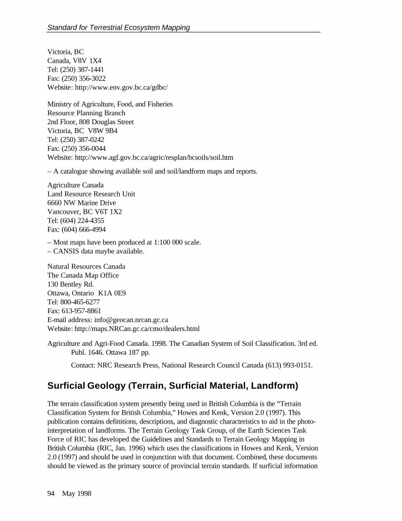
Standard for Terrestrial Ecosystem Mapping
94 May 1998
Victoria, BCCanada, V8V 1X4Tel: (250) 387-1441Fax: (250) 356-3022Website: http://www.env.gov.bc.ca/gdbc/
Ministry of Agriculture, Food, and FisheriesResource Planning Branch2nd Floor, 808 Douglas StreetVictoria, BC V8W 9B4Tel: (250) 387-0242Fax: (250) 356-0044Website: http://www.agf.gov.bc.ca/agric/resplan/bcsoils/soil.htm
– A catalogue showing available soil and soil/landform maps and reports.
Agriculture CanadaLand Resource Research Unit6660 NW Marine DriveVancouver, BC V6T 1X2Tel: (604) 224-4355Fax: (604) 666-4994
– Most maps have been produced at 1:100 000 scale.– CANSIS data maybe available.
Natural Resources CanadaThe Canada Map Office130 Bentley Rd.Ottawa, Ontario K1A 0E9Tel: 800-465-6277Fax: 613-957-8861E-mail address: [email protected]: http://maps.NRCan.gc.ca/cmo/dealers.html
Agriculture and Agri-Food Canada. 1998. The Canadian System of Soil Classification. 3rd ed.Publ. 1646. Ottawa 187 pp.
Contact: NRC Research Press, National Research Council Canada (613) 993-0151.
Surficial Geology (Terrain, Surficial Material, Landform)
The terrain classification system presently being used in British Columbia is the “TerrainClassification System for British Columbia,” Howes and Kenk, Version 2.0 (1997). Thispublication contains definitions, descriptions, and diagnostic characteristics to aid in the photo-interpretation of landforms. The Terrain Geology Task Group, of the Earth Sciences TaskForce of RIC has developed the Guidelines and Standards to Terrain Geology Mapping inBritish Columbia (RIC, Jan. 1996) which uses the classifications in Howes and Kenk, Version2.0 (1997) and should be used in conjunction with that document. Combined, these documentsshould be viewed as the primary source of provincial terrain standards. If surficial information

Appendix B: Data Sources
May 1998 95
has already been mapped for a project area, it appropriateness will need to be assessed inrelation to the objectives and standards of the current project.
Surficial Geology maps are available from a wide variety of sources and are described in anequally disparate manner, a few of which are listed below. A discussion of the descriptionsand sources can be found in RIC Jan. 1996.
Ministry of Employment and InvestmentGeological Survey BranchPO Box 9320, Stn Prov Gov’tVictoria, BC V8W 9N3Tel: (250) 952-0429Fax: (250) 952-0381Website: http://www.ei.gov.bc.ca/geosmin/mapinv/surfical.htm
– Historical bedrock information– Digital Terrain and/or Soils and Landform maps available at 1:20 000, 1:50 000 1:100 000
and/or 1:250 000.
Natural Resources CanadaGeologic Survey of Canada101 – 605 Robson StreetVancouver, BCTel: (604) 666-0529Fax: (604) 666-1337 (sales)
Crown Publications Inc.521 Fort StreetVictoria, BC V8W 1E7Tel: (250) 386-4636Fax: (250) 386-0221E-mail address: [email protected]: http://vvv.com/crownpub/
– Provides information on bedrock and surficial materials produced federally and provincially.– An index of the reports and maps produced for BC is updated periodically
Topography
Topographic maps are available at a variety of scales (1:20 000, 1:50 000, 1:100 000,1:250 000) for the province and are usually gridded using the NTS (National TopographicalSystem) and the BCGS (British Columbia Geographic System). UTM and Latitude/ Longitudegrids are usually included on these maps. For the purposes of Terrestrial Ecosystem Mapping,BCGS maps are preferred.
TRIM (Terrain Resource Information Mapping ) maps and reports at 1:20 000 and Ministry ofEnvironment maps at 1:250 000 can be ordered from Geographic Data BC. TRIM maps at1:50 000 for selected areas are also available from the Ministry of Forests, Forest Practices

Standard for Terrestrial Ecosystem Mapping
96 May 1998
Branch. Where available , TRIM maps should be used as the standard for topographicinformation.
Ministry of Environment, Lands, and ParksGeographic Data BC BranchCustomer Support3rd. Fl., 1802 Douglas St.,Victoria, BCCanada, V8V 1X4Tel: (250) 387-1441Fax: (250) 356-3022Website: http://www.env.gov.bc.ca/gdbc/
– 1:20000 TRIM maps available
Ministry of ForestsForest Practices BranchP.O. Box 9513, Stn. Prov. Gov’tVictoria, BC V8W 9C3Tel: (250) 387-6656Fax: (250) 387-6751
Crown Publications Inc.521 Fort StreetVictoria, BC V8W 1E7Tel: (250) 386-4636Fax: (250) 386-0221E-mail address: [email protected]: http://vvv.com/crownpub/
– 1:50 000 NTS maps available
Natural Resources CanadaThe Canada Map Office130 Bentley Rd.Ottawa, Ontario K1A 0E9Tel: 800-465-6277Fax: 613-957-8861E-mail address: [email protected]: http://maps.NRCan.gc.ca/cmo/dealers.html
Vegetation
Vegetation maps, including forest cover maps, are used to aid in the delineation of map unitsbased on major vegetation and stand structure attributes. Vegetation maps have beenproduced in the past at a variety of scales by variety of sources, including the Ministry ofEnvironment. Some of these maps may be available from Geographic Data BC. Furtherinformation on vegetation can be gathered from forest cover maps, such as tree species, standage, and disturbance history. With the implementation of the new Ministry of Forests

Appendix B: Data Sources
May 1998 97
Vegetation Resources Inventory, information on understory vegetation, structural stages,coarse woody debris, and snags will also be available.
Forest Cover Maps are available in hardcopy or digital form from Ministry of Forests. ForestCover maps can also be accessed as digital files off of the BCSYS Network.
Ministry of ForestsResources Inventory BranchDigital Data Sales Distribution CentrePO Box 9516, Stn Prov Gov’tVictoria, BC V8W 9C2Tel: (250) 387-1314Fax: (250) 387-5999Website: http://www.for.gov.bc.ca/resinv/products/DigData/brochure.htm
– Forest Cover information is also available from the Ministry of Forests District offices.
Ministry of Forests, Resources Tenure and Engineering BranchPO Box 9510, Stn Prov Gov’tVictoria, BC V8W 9C2Tel: (250) 387-5291Fax: (250) 387-6445Website: http://www.for.gov.bc.ca/RTE/rtehome.htm
– Forest Atlas (1:20000 scale) provides spatial information regarding forest tenures, forestryand logging roads, trails, harvesting history, and gravel pits.
Database Formats
Ecosystem map database manuals, including formats for polygon database development andfor GIS specifications have been developed by the Ministry of Environment, Lands, and Parksand are available on the ftp site. These manuals outline the standards and procedures forcapturing, storing, and distributing ecological and terrain data for GIS as well as otherdatabase systems.
Currently there is a database and analysis package for field data available; it is called VENUS(Vegetation and Environmental data NexUS). The current version is 3.0 but the programcould be subject to change so the TEM website should be consulted for the latest version ofVENUS. Further information regarding the VENUS 3.0 or earlier versions of the VENUSdata entry program and tabling software, can be obtained from:
Ministry of Forests ftp site:IP address: 142.36.191.210UserId: anonymousPassword: guestThe ftp directory is pub/VENUS
OR
URL address: ftp://cowichan.for.gov.bc.ca/pub/VENUS

Standard for Terrestrial Ecosystem Mapping
98 May 1998
OR
TEM website:http://www.env.gov.bc.ca/rib/wis/tem
If you encounter problems downloading the program or entering data, or simply have questionsregarding VENUS, please contact Greg Britton, Ecology Data Analyst, at the ResearchBranch, Ministry of Forests.
Tel:(250) 387-6717.Fax: (250) 387-0046e-mail address: [email protected]
Resources Inventory Committee. 1997. Data Standards for Terrestrial Ecosystem Mapping inBritish Columbia. Resources Inventory Committee, Victoria, BC.
Contact: Ministry of EnvironmentTEM website: http://www.env.gov.bc.ca/rib/wis/tem
Data Forms
Guidelines for the field collection of ecological data has been well documented in the FieldManual for Describing Terrestrial Ecosystems (BC Ministry of Forests and BC Ministry ofEnvironment, 1998a). This document includes information, guidelines, and field forms (FS882)required for coarse woody debris and wildlife tree data collection, along with site, soil,vegetation, mensuration, and wildlife habitat data collection. There is also a revised field formfor doing ground inspections, and visual checks. This form is called the Ground InspectionForm (GIF).
The above data collection guidelines and the associated field forms should be viewed as thestandard for all ecological data collection in the field. Information about ordering thesedataforms can be found on the TEM website.
Other Data Sources
The list of potential sources of data useful for ecological mapping is extensive. The above listcomprises the recommended data sources for some of the primary data needs of ecologicalmapping projects.
Web browsers are also available which provide further information regarding the differentmap products and publications that are available, along with their sources.
These include:
Geographic Data BC Branch site at: http://www.env.gov.bc.ca/gdbc/Land Data BC site at: http://www.landdata.gov.bc.ca/Resources Inventory Committee at: http://www.for.gov.bc.ca/RIC

Appendix C: Natural Disturbance Types
May 1998 99
Appendix C: Natural Disturbance Types
Natural disturbance types (NDTs) as outlined in the Forest Practices Code BiodiversityGuidelines (1995) characterize areas with different natural disturbance regimes. Naturaldisturbance regimes include fire, wind, insects and disease. The following five naturaldisturbance regimes are recognized in the Forest Practices Code Biodiversity Guidebook:
NDT DefinitionNDT1 Ecosystems with rare stand-initiating eventsNDT2 Ecosystems with infrequent stand-initiating eventsNDT3 Ecosystem with frequent stand-initiating eventsNDT4 Ecosystem with frequent stand-maintaining eventsNDT5 Alpine Tundra and Subalpine Parkland ecosystems
All of the Biogeoclimatic subzones and variants recognized provincially have been classed intoone of the above natural disturbance types. These natural disturbance types have been usedin the Standard for Terrestrial Ecosystem Mapping to help define structural stages for matureand old forests. This document recognizes that because of their frequent stand initiatingevents, ecosystems falling under NDT3 should be considered mature and old sooner than allof the other NDTs. As outlined in Table 3.3, ecosystems falling within the Biogeoclimaticsubzones/variants listed under NDT3 are recognized as being mature starting at 80–120 years,and old at greater than 140 years (100 years for BWBS). Other ecosystems within NDT1,NDT2, NDT 4 and NDT5 are considered mature starting at 80–120 years, and old greaterthan 250 years. For simplification the table below lists all subzone/variants recognized underNDT3, and calls them Subzone Group A. All subzone/variants recognized under NDT1,NDT2, NDT 4 and NDT5 are listed under, Subzone Group B.

Standard for Terrestrial Ecosystem Mapping
100 May 1998
GROUP A & B BIOGEOCLIMATIC ZONES IN BRITISH COLUMBIA
Group A Subzones: NDT1 Group B Subzones: NDT2, 3, 4, & 5Zones (Old at greater than 140 years.) (Old at greater than 250 years.)
BG BGxh (all variants) BGxw (all variants)BWBS BWBSdk (all variants) BWBSvk
BWBSmw (all variants) BWBSwk (all variants)CDF CDFmmCWH CWHdm CWHwm
CWHds (all variants) CWHws (all variants)CWHmm (all variants) CWHvh (all variants)CWHms (all variants) CWHvm (all variants)CWHwh (all variants) CWHxm (all variants)
ESSF ESSFdc (all variants) ESSFdv ESSFmc ESSFwk (all variants)ESSFdk ESSFxc ESSFmk ESSFwv
ESSFmm (all variants) ESSFvcESSFmw ESSFvv
ESSFmv (all variants) ESSFxv ESSFwm All ESSF parkland variants ESSFwc (all variants)
ICH ICHdk ICHmk2 ICHmm ICHwcICHdw ICHmw3 ICHmc (all variants) ICHwk (all variants)ICHmk1 ICHmk3 ICHvc
ICHmw1 ICHvk (all variants)ICHmw2 ICHxw
IDF IDFdk (all variants) IDFxh (all variants)IDFdm (all variants) IDFxmIDFmw (all variants) IDFxwIDFww
MH MHmm (all variants)MHwh (all variants)All MH parkland variants
MS MSdc MSxkMSdk MSxvMSdm (all variants)
PP PPdh (all variants) PPxh (all variants)SBPS SBPSdc SBPSmk
SBPSmc SBPSxcSBS SBSdh (all variants) SBSmk (all variants) SBSwk1 mountain SBSvk
SBSdk SBSmm SBSwk2SBSdw (all variants) SBSmwSBSmc (all variants) SBSwk1 plateauSBSmh SBSwk3
SWB SWBdk SWBmksSWBmk SWBvksSWBdks