stable operations in generalized cohomologyhopf.math.purdue.edu/boardman/stabop.pdf1 introduction 1...

Stable Operations in Generalized Cohomology

J. Michael Boardman

January 1995

[To appear in Handbook of Algebraic Topology,ed. I. M. James, Elsevier (Amsterdam, 1995)]

TABLE OF CONTENTS

1 Introduction 1

2 Notation and five examples 3

3 Generalized cohomology of spaces 6

4 Generalized homology and duality 13

5 Complex orientation 16

6 The categories 21

7 Algebraic objects in categories 28

8 What is a module? 35

9 E-cohomology of spectra 43

10 What is a stable module? 50

11 Stable comodules 56

12 What is a stable algebra? 64

13 Operations and complex orientation 71

14 Examples of ring spectra for stable operations 73

15 Stable BP -cohomology comodules 83

Index of symbols 87

References 89

1 Introduction

For any space X, the Steenrod algebra A of stable cohomology operations acts onthe ordinary cohomology H∗(X;Fp) to make it an A-algebra. Milnor discovered [22]that it is useful to treat H∗(X;Fp) as a comodule over the dual of A, which becomesa Hopf algebra. Adams extended this program in [1, 3] to multiplicative generalizedcohomology theories E∗(−), under appropriate hypotheses. The coefficient ring E∗

is now graded, and E∗(X) is an E∗-algebra.Our purpose is to describe the structure of the stable operations on E∗(−) in a

manner that will generalize in [9] to unstable operations. Unlike some treatments, we

JMB – 1 – 23 Feb 1995

Stable cohomology operations

impose no finiteness or connectedness conditions whatever on the spaces and spectrainvolved, only a single freeness condition on E. We emphasize universal propertiesas the appropriate setting for many results. An early version of some of the ideas ispresented in [8], which is limited to ordinary cohomology, MU , and BP .

For general E, the stable operations form the endomorphism ring A = E∗(E, o)of E (in our notation). For each x ∈ E∗(X), we have the E∗-module homomorphismx∗:A → E∗(X) given by x∗r = ± rx. The key idea is (roughly) that given an E∗-module M , we define SM as the set of all E∗-module homomorphisms A → M ; thisis to be thought of as the set of candidates for the values of all operations on a typicalelement of M .

Generally, we encode the action of A on a stable module M as the functionρM :M → SM given by (ρMx)r = ± rx. There is an E∗-module structure on SM

(different from the obvious one) that makes ρM a homomorphism of E∗-modules. Thisis not yet enough; composition of operations makes the functor S what is known asa comonad , and we need (M, ρM ) to be a coalgebra over this comonad. When M isan E∗-algebra, so is SM , and we can similarly define stable algebras.

This work serves as more than just a pattern for the promised unstable theory of[9]. To compare unstable structures with the analogous stable structures, we shallthere construct suitable natural transformations; this is far easier to do when boththeories are developed in the same manner. Much of the basic category theory is thesame for either case; we keep it all here for convenience. Finally, we need specificstable results for later use.

Outline In §2, we introduce five assorted ring spectra E, which will serve through-out as our examples. We review some elementary category theory and set up notation.

In §§3, 4, we study E-(co)homology in enough detail to suggest what categories touse. In §9, we consider (co)homology in the stable homotopy category of spectra. Itis essential for us to work in the correct categories, in order to make our categoricalmachinery run smoothly; otherwise it does not run at all. We therefore take pains in§6 to say precisely what our categories are.

In §7, we discuss the various kinds of algebraic object, such as group, module, andring, that we need in general categories. In §8, we rework the definition of a moduleover a ring until we find a way that will generalize to the unstable context.

In §10, we discuss stable modules from several points of view. We introduce thecomonad S, and define a stable module as an S-coalgebra. Theorem 10.16 shows thatE∗(X) is (more or less) a stable module.

In §11, we make the homology E∗(E, o) a coalgebra (in a sense), provided onlythat it is a free E∗-module. A stable module then becomes a comodule over it;indeed, Thm. 11.13 shows that the theories of stable modules and stable comodules areentirely equivalent. Theorem 11.14 provides a useful universal property of E∗(E, o).Theorem 11.35 shows that our structure on E∗(E, o) agrees with that introduced byAdams [1].

Everything mentioned so far works for spectra X, too. In §12, we take account ofthe multiplication present on E∗(X) when X is a space by making SM an E∗-algebrawhenever M is. This leads to the definition of a stable algebra. Again, there is an

JMB – 2 – 23 Feb 1995

§2. Notation and five examples

equivalent comodule version.All our examples of E-cohomology come with a complex orientation. This has

standard implications for the structure of E∗(CP∞) etc., which we review in §5. In§13, we study the consequences for operations.

In §14, we present the structure on E∗(E, o) in detail for each of our five examplesE. We do not actually construct the operations, which are all well known. It is clearthat many other examples are available.

In §15, we study the special case of BP -cohomology in greater depth. For ageneral introduction, see Wilson [37]. Stable BP -operations are well established; ashort early history would include Landweber [17], Novikov [28], Quillen [30], Adams[3], Zahler [41, 42], Miller-Ravenel-Wilson [21], and more recently, Ravenel’s book[31]. We review Landweber’s filtration theorem, for imitation in [9].

An index of symbols is included at the end.

Acknowledgements We thank Dave Johnson and Steve Wilson for making thispaper necessary. As noted, it serves chiefly as a platform for [9]. It incorporatesseveral suggestions of Steve Wilson, especially the use of corepresented functors in§8. We also thank Nigel Ray for pointing out some useful references.

2 Notation and five examples

Our five examples of commutative ring spectra E are:

H(Fp) The Eilenberg-MacLane spectrum, for a fixed prime p ≥ 2, which representsordinary cohomology H∗(−;Fp) and is a ring spectrum (see e. g. Switzer [34,13.88]);

BP The Brown-Peterson spectrum, for a fixed prime p ≥ 2 (which is suppressedfrom the notation), a ring spectrum by Quillen [29];

MU The unitary (or complex) cobordism Thom spectrum, which is a ring spec-trum (see e. g. Switzer [34, 13.89]);

KU The complex Bott spectrum (often written K), which represents topologicalcomplex K-theory and is a ring spectrum [ibid., 13.90];

K(n) The Morava K-theory spectrum, for a fixed prime p > 2 (again suppressedfrom the notation), and any n ≥ 0. (We take p > 2 in order to ensure thatthe multiplication is commutative as well as associative; see Morava [26],and especially Shimada-Yagita [33, Cor. 6.7] or Wurgler [38, Thm. 2.14].See [16] for background information.)

In particular, K(0) = H(Q) (for any p), and K(1) is a summand of KU-theory mod p.

Indeed, all our ring spectra are understood to be commutative. Each E definesa multiplicative cohomology theory E∗(X) and homology theory E∗(X), which wediscuss in §§3, 4. They have the same coefficient ring E∗.

Because we deal almost exclusively in cohomology, we assign the degree n tocohomology classes in En(X) and elements of En; this forces homology classes in

JMB – 3 – 23 Feb 1995


En(X) to have degree −n. Note that under this convention, elements of BP ∗ andMU∗ are given negative degrees.

For any space X, E∗(X) and E∗(X) are E∗-modules. We therefore adopt E∗ as ourground ring throughout, and all tensor products and groups Hom(M,N) are takenover E∗ unless otherwise specified. Except for (co)homology, we generally follow thepractice of [25] in writing a graded group with components Mn as M rather than M∗.When we do write M∗ (e. g. E∗ as above), we mean the whole graded group, not atypical component.

All our rings and algebras are associative and are presumed to have a unit element1, which is to be preserved by homomorphisms. Dually, coalgebras are assumed tobe coassociative.

Summations are often understood as taken over all available values of the index.We do not attempt to give each construct a unique symbol. For example, all mul-

tiplications are named φ, which we decorate as φS etc. only as needed to distinguishdifferent multiplications. All actions are named λ and all coactions are named ρ. Tocompensate, we generally specify where each equation takes place.

Signs We follow the convention that a minus sign should be introduced whenevertwo symbols of odd degree become transposed for any reason. As explained in [7],this is a purely lexical convention, which depends only on the order of appearanceof the various symbols, not on their meanings. The principle is that consistency willbe maintained provided one starts from equations that conform and performs only“reasonable” manipulations on them. The main requirement is that each symbolhaving a degree should appear exactly once in every term of an equation.

Category theory Our basic reference is MacLane’s book [20], which also providesmost of our notation and terminology.

In any category A, the set of morphisms from X to Y is denoted A(X, Y ), or occa-sionally Mor(X, Y ). If A is a graded category (always assumed additive), An(X, Y )denotes the abelian group of morphisms from X to Y of degree n. Unmarked ar-rows are intended to be the obvious morphisms. We write p1:X × Y → X andp2:X × Y → Y for the projections from the product X × Y to its factors, and duallyi1:X → X q Y and i2:Y → X q Y for coproducts. We also write q:X → T for theunique morphism to a terminal object T .

We denote by I:A→ A the identity functor of A. We sometimes find it useful towrite a natural transformation α between functors F, F ′:A → B as

α:F → F ′:A → B .If A and B are graded, we can have deg(α) = m 6= 0; in this case, we requireαY Ff = (−1)mdeg(f)F ′f αX for each morphism f :X → Y . In contrast, ourgraded functors invariably preserve degree.

If α′:F ′ → F ′′ is another natural transformation, we have the composite naturaltransformation α′ α:F → F ′′. There is the identity natural transformation 1: F →F . Given also G:B → C, we denote the composite functor as GF :A → C (neverG F ), and define the natural transformation Gα:GF → GF ′:A → C by (Gα)X =G(αX). Similarly, given β:G→ G′, we define βF :GF → G′F :A → C by (βF )X =

JMB – 4 – 23 Feb 1995

§2. Notation and five examples

β(FX). We also have βα = βF ′ Gα = G′α βF :GF → G′F ′:A → C (or ±G′α βFin the graded case).

We make incessant use of Yoneda’s Lemma [20, III.2].

Adjoint functors It should be no surprise that we have numerous pairs of adjointfunctors. Suppose given a functor V :B → A (which is usually, but not necessarily,some forgetful functor) and an object A in A.

Definition 2.1 We call an object M in B V-free on A, with basis i:A → VM , amorphism in A, if for each B in B, any morphism f :A → V B in A “extends” toa unique morphism g:M → B in B, called the left adjunct of f , in the sense thatV g i = f :A→ V B.

In the language of [20, III.1], i is a universal arrow , which induces the bijectionB(M,B) ∼= A(A, V B). The free object M is unique up to canonical isomorphism,but there is no guarantee that one exists. In the favorable case when we have a freeobject FA for each A in A, with basis ηA:A→ V FA, there is a unique way to defineFh for each morphism h in A to make η natural; then F becomes a functor and theisomorphism

B(FA,B) ∼= A(A, V B), (2.2)

is natural in both A and B. Explicitly, we recover f :A→ V B from g:FA→ B as

f = V g ηA:A −−→ V FA −−→ V B in A. (2.3)

For any B, we define εB:FV B → B in B as extending 1:V B → V B. Thenε:FV → I is also natural, and we may construct the left adjunct g of f as

g = εB Ff :FA −−→ FV B −−→ B in B. (2.4)

The fact that this is inverse to eq. (2.3) is neatly expressed by the pair of identities

(i) V ε ηV = 1:V −−→ V :B −−→ A(ii) εF Fη = 1:F −−→ F :A −−→ B

(2.5)

We summarize the basic facts about adjoint functors from [20, Thm. IV.1.2].

Theorem 2.6 The following conditions on a functor V :B → A are equivalent:

(i) V has a left adjoint F :A → B;

(ii) V is a right adjoint to some functor F :A→ B;

(iii) There is a functor F :A → B and an isomorphism (2.2), natural in A andB;

(iv) For all A in A, we can choose a V-free object FA and a basis ηA of it;

(v) There is a functor F :A → B with natural transformations η: I → V F andε:FV → I that satisfy eqs. (2.5).

In view of the symmetry in (v), or between (i) and (ii), we have the dual result,which we do not state. Nevertheless, we do give the dual to Defn. 2.1.

Definition 2.7 The object N in B is V-cofree on A, with cobasis p:V N → A,a morphism in A, if for each B in B, any f :V B → A in A “lifts” uniquely to amorphism g:B → N in B, called the right adjunct of f , in the sense that p V g = f .

JMB – 5 – 23 Feb 1995


3 Generalized cohomology of spaces

In this section and the next, we review multiplicative cohomology theories E∗(−)and their associated homology theories E∗(−) in sufficient depth to decide what ob-jects our categories should contain. We also establish much of our notation.

Spaces We find we have to work mostly with unbased spaces. The most convenientspaces are CW-complexes. We denote by T the one-point space. It is sometimes usefulto allow also spaces that are homotopy equivalent to CW-complexes, so that we canform products and loop spaces directly. A pair (X,A) of spaces is assumed to be aCW-pair (or homotopy equivalent, as a pair, to one).

Ungraded cohomology For our purposes, an ungraded cohomology theory is ahomotopy-invariant contravariant functor h(−) that assigns to each space X anabelian group h(X), and satisfies the usual two axioms:

(i) h(−) is half-exact: If X = A∪B, where A and B are well-behavedsubspaces (e.g. subcomplexes of a CW-complex X), and y ∈ h(A)and z ∈ h(B) agree in h(A ∩ B), there exists x ∈ h(X) (not ingeneral unique) that lifts both y and z;

(ii) h(−) is strongly additive: For any topological disjoint union X =∐αXα, the inclusions Xα ⊂ X induce h(X) ∼= ∏

α h(Xα).

(3.1)

For a space X with basepoint o ∈ X, we may define the reduced cohomologyh(X, o) by the split short exact sequence

0 −−→ h(X, o)⊂−−→ h(X) −−→ h(o) −−→ 0. (3.2)

We recover the absolute cohomology h(X) by constructing the disjoint union X+ ofX with a (new) basepoint; by (ii), h(X+) ∼= h(X)⊕ h(o) and the inclusion X ⊂ X+

induces an isomorphismh(X+, o) ∼= h(X) . (3.3)

For a good pair (X,A) of spaces, we may define the relative cohomology as

h(X,A) = h(X/A, o), (3.4)

and these groups behave as expected. We generalize eq. (3.2).

Lemma 3.5 If A is a retract of X, we have the split short exact sequence

0 −−→ h(X,A) −−→ h(X) −−→ h(A) −−→ 0.

If A has a basepoint o, we have also the split short exact sequence

0 −−→ h(X,A) −−→ h(X, o) −−→ h(A, o) −−→ 0.

With no basepoints, we have to be a little careful in representing h(−). Let Ho bethe homotopy category of spaces that are (homotopy equivalent to) CW-complexes.

Theorem 3.6 Let h(−) be an ungraded cohomology theory as above. Then:

(a) h(−) is represented in Ho by anH-space H, with a universal class ι ∈ h(H, o) ⊂h(H) that induces an isomorphism Ho(X,H) ∼= h(X) of abelian groups by f 7→ h(f)ιfor all X;

JMB – 6 – 23 Feb 1995

§3. Generalized cohomology of spaces

(b) For any cohomology theory k(−), operations θ:h(−) → k(−) correspond toelements θι ∈ k(H).

Proof What Brown’s representation theorem [10, Thm. 2.8, Ex. 3.1] actually pro-vides is a based connected space (H ′, o), which represents h(−, o) on based connectedspaces (X, o) only. Then West [35] shows that h(−, o) is represented on all basedspaces by the product space

H = h(T )×H ′, (3.7)

where we treat the group h(T ) as a discrete space. By eq. (3.3), H also representsh(−) in the unbased category Ho.

The map ω:T → H that corresponds to 0 ∈ h(T ) furnishes H with a (homotopi-cally well-defined) basepoint, and the exact sequence (3.2) shows that ι ∈ h(H, o).Yoneda’s Lemma represents the addition

Ho(X,H×H) ∼= h(X)× h(X)+−−→ h(X) ∼= Ho(X,H)

by an addition map µ:H ×H → H which makes H an H-space, and also gives (b).(Lemma 7.7(a) will tell us much more about H.)

Example: KU For finite-dimensional spaces X, the ungraded cohomology theoryKU(X) is defined (e. g. Husemoller [15]) as the Grothendieck group of complex vectorbundles over X. The class of the vector bundle ξ is denoted [ξ], and every elementof KU(X) has the form [ξ] − [η]. The trivial n-plane bundle is denoted simply n.Addition is defined from the Whitney sum of vector bundles, [ξ] + [η] = [ξ ⊕ η], andmultiplication from the tensor product, [ξ][η] = [ξ ⊗ η]. In particular, KU(T ) ∼= Z,as a ring.

Let (X, o) be a based connected space, still finite-dimensional. Because any vectorbundle ξ over X has a stable inverse η such that ξ ⊕ η is trivial, every element ofKU(X, o) can be written in the form [ξ]−n for some n-plane vector bundle ξ, providedn is large enough. The bundle ξ has a classifying map X → BU(n) ⊂ BU , whichleads to the representation Ho(X,BU) ∼= KU(X, o). As in the proof of Thm. 3.6, thisextends to an isomorphism Ho(X,Z×BU) ∼= KU(X), valid for all finite-dimensionalspaces X.

To extend KU(−) to all spaces as an ungraded cohomology theory, we must defineKU(X) = Ho(X,Z×BU). It remains true that any vector bundle ξ over X definesan element [ξ] ∈ KU(X), but in general, not all elements of KU(X) have the form[ξ]− [η].

Splittings All our splittings depend on the following elementary result.

Lemma 3.8 Assume that θ:h(−) → h(−) is an idempotent cohomology operation,θ θ = θ. Then the image θh(−) also satisfies the axioms (3.1).

Proof For (i), given y ∈ θh(A) and z ∈ θh(B) that agree in h(A ∩ B), the half-exactness of h yields an element x ∈ h(X) that lifts y and z. Because θ is idempotent,θx ∈ θh(X) also lifts y and z, to show that (i) holds.

For (ii), we need only the naturality of θ. Given elements xα = θx′α ∈ θh(Xα),axiom (ii) for h provides x′ ∈ h(X) that lifts each x′α. Then x = θx′ ∈ θh(X) liftseach xα, and is unique because h satisfies (ii).

JMB – 7 – 23 Feb 1995


We immediately deduce the standard tool for constructing splittings. Theorem3.6(b) allows us to write the identity operation as ι.

Lemma 3.9 Let θ be an additive idempotent operation on the ungraded cohomologytheory h(−). Then:

(a) ι− θ is also idempotent;

(b) We can define ungraded cohomology theories

h′(X) = Ker[θ:h(X) −−→ h(X)] = Im[ι− θ:h(X) −−→ h(X)]

andh′′(X) = Ker[ι− θ:h(X) −−→ h(X)] = Im[θ:h(X) −−→ h(X)];

(c) We have the natural direct sum decompositon h(X) = h′(X)⊕ h′′(X);

(d) If the H-spaces H ′ and H ′′ represent h′(−) and h′′(−) as in Thm. 3.6(a), thenH ′ ×H ′′ represents h(−).

For future use in [9], we extend this result to certain nonadditive idempotentoperations. To emphasize the nonadditivity, we retain the parentheses in θ(−).

Lemma 3.10 Assume the nonadditive operation θ on the ungraded cohomology the-ory h(−) satisfies the axioms:

(i) θ(0) = 0;

(ii) θ(x+ y − θ(y)) = θ(x) for any x, y ∈ h(X).(3.11)

Then:

(a) θ and ι− θ are idempotent;

(b) We can define the kernel cohomology theory h′(−) = Ker θ = Im(ι−θ) as asubgroup of h(−);

(c) We can define the coimage cohomology theory h′′(X) = Coim θ = h(X)/h′(X)as a quotient of h(X), with projection π:h(X)→ h′′(X);

(d) We have the natural short exact sequence of ungraded cohomology theories

0 −−→ h′(X)⊂−−→ h(X)

π−−→ h′′(X) −−→ 0; (3.12)

(e) θ induces a nonadditive operation θ:h′′(X) → h(X) which splits (3.12) andinduces the bijection of sets h′′(X) = Coim θ ∼= Im[θ:h(X)→ h(X)];

(f) The short exact sequence (3.12) is represented by a fibration of H-spaces andH-maps

H ′ −−→ H −−→ H ′′

in which H → H ′′ admits a section (not an H-map) and H ' H ′ ×H ′′ as spaces.

Remark Note the asymmetry of the situation. It is necessary to distinguish (cf. [20,VIII.3]) between the coimage of θ, which is a quotient group of h(X), and the imageof θ, which in interesting cases is only a subset of h(X), not a subgroup (otherwiseLemma 3.9 would be available).

Proof For (a), we put x = θ(y) in (ii) to see that θ is idempotent. If we put x = 0instead, we see that θ(y − θ(y)) = 0, which implies that ι− θ is idempotent.

JMB – 8 – 23 Feb 1995


For (b), we have just seen that Im(ι−θ) ⊂ Ker θ. The opposite inclusion is trivial,because if θ(x) = 0, we can write x = (ι−θ)(x).

To see that h′(X) is a subgroup, we first note that 0 ∈ h′(X) by (i). Take anyz ∈ h′(X), which we may write as z = y − θ(y). Then by (ii), x + z ∈ h′(X) if andonly if x ∈ h′(X). Therefore by Lemma 3.8 (which did not require θ to be additive),h′(−) is a cohomology theory.

This allows us to define the coimage h′′(X) in (c) as an abelian group. By (ii) and(b), θ in (e) is well defined and provides the inverse bijection to Im θ ⊂ h(X)→ h′′(X).By Lemma 3.8, Im θ and hence h′′(−) satisfy the axioms (3.1), and h′′ is a cohomologytheory. Then (d) combines (b) and (c).

For (f), we represent π by a fibration H → H ′′, which is an H-map of H-spaces.Then θ is represented by a section. It follows from the short exact sequence (3.12)that the fibre of π represents h′.

Graded cohomology A graded cohomology theory E∗(−) consists of an ungradedcohomology theory En(−) for each integer n, connected by natural suspension iso-morphisms

Σ:En(X) ∼= En+1(S1 ×X, o×X) (3.13)

of abelian groups, much as in Conner-Floyd [12, §4]. By Lemma 3.5, there is a splitshort exact sequence

0 −−→ En+1(S1×X, o×X) −−→ En+1(S1×X) −−→ En+1(o×X) −−→ 0. (3.14)

For a based space (X, o), Σ induces, with the help of eq. (3.4), the commutativediagram of split exact sequences

En(X, o) En(X) En(o)

En+1(ΣX, o) En+1

(S1×Xo×X , o

)En+1(S1×o, o)

-p

p

p

p

p

p

p

p

p?

∼= Σ

-

?

∼= Σ

?

∼= Σ

- -

(3.15)

whose bottom row comes from Lemma 3.5, where the suspension of X is

ΣX = S1 ∧X =S1×XS1 ∨X

∼= S1×Xo×X

/S1×o .

We deduce the more commonly used reduced suspension isomorphism Σ:En(X, o) ∼=En+1(ΣX, o). In view of eq. (3.3), we recover eq. (3.13) as a special case.

By iteration of eq. (3.13), or analogy, there are k-fold suspension isomorphisms forall k > 0

Σk:En(X) ∼= En+k(Sk ×X, o×X) . (3.16)

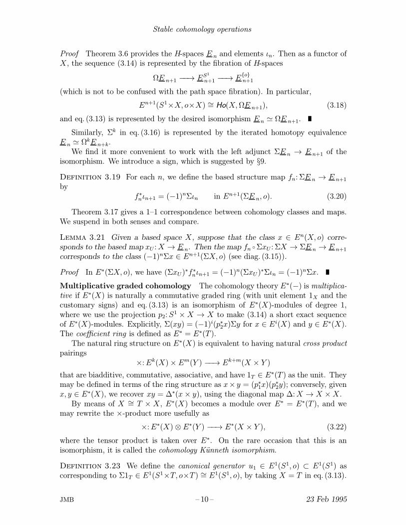
Theorem 3.17 Any graded cohomology theory E∗(−) is represented in Ho by anΩ-spectrum n 7→ E n, consisting of H-spaces E n equipped with universal elementsιn ∈ En(E n, o) ⊂ En(E n) and isomorphisms (in Ho) of H-spaces E n ' ΩE n+1.

JMB – 9 – 23 Feb 1995


Proof Theorem 3.6 provides the H-spaces E n and elements ιn. Then as a functor ofX, the sequence (3.14) is represented by the fibration of H-spaces

ΩE n+1 −−→ ES1

n+1 −−→ Eon+1

(which is not to be confused with the path space fibration). In particular,

En+1(S1×X, o×X) ∼= Ho(X,ΩE n+1), (3.18)

and eq. (3.13) is represented by the desired isomorphism E n ' ΩE n+1.

Similarly, Σk in eq. (3.16) is represented by the iterated homotopy equivalenceE n ' ΩkE n+k.

We find it more convenient to work with the left adjunct ΣE n → E n+1 of theisomorphism. We introduce a sign, which is suggested by §9.

Definition 3.19 For each n, we define the based structure map fn: ΣE n → E n+1

byf ∗nιn+1 = (−1)nΣιn in En+1(ΣE n, o). (3.20)

Theorem 3.17 gives a 1–1 correspondence between cohomology classes and maps.We suspend in both senses and compare.

Lemma 3.21 Given a based space X, suppose that the class x ∈ En(X, o) corre-sponds to the based map xU :X → E n. Then the map fn ΣxU : ΣX → ΣE n → E n+1

corresponds to the class (−1)nΣx ∈ En+1(ΣX, o) (see diag. (3.15)).

Proof In E∗(ΣX, o), we have (ΣxU )∗f ∗nιn+1 = (−1)n(ΣxU )∗Σιn = (−1)nΣx.

Multiplicative graded cohomology The cohomology theory E∗(−) is multiplica-tive if E∗(X) is naturally a commutative graded ring (with unit element 1X and thecustomary signs) and eq. (3.13) is an isomorphism of E∗(X)-modules of degree 1,where we use the projection p2:S1 ×X → X to make (3.14) a short exact sequenceof E∗(X)-modules. Explicitly, Σ(xy) = (−1)i(p∗2x)Σy for x ∈ Ei(X) and y ∈ E∗(X).The coefficient ring is defined as E∗ = E∗(T ).

The natural ring structure on E∗(X) is equivalent to having natural cross productpairings

×:Ek(X)× Em(Y ) −−→ Ek+m(X × Y )

that are biadditive, commutative, associative, and have 1T ∈ E∗(T ) as the unit. Theymay be defined in terms of the ring structure as x× y = (p∗1x)(p∗2y); conversely, givenx, y ∈ E∗(X), we recover xy = ∆∗(x× y), using the diagonal map ∆:X → X ×X.

By means of X ∼= T × X, E∗(X) becomes a module over E∗ = E∗(T ), and wemay rewrite the ×-product more usefully as

×:E∗(X)⊗ E∗(Y ) −−→ E∗(X × Y ), (3.22)

where the tensor product is taken over E∗. On the rare occasion that this is anisomorphism, it is called the cohomology Kunneth isomorphism.

Definition 3.23 We define the canonical generator u1 ∈ E1(S1, o) ⊂ E1(S1) ascorresponding to Σ1T ∈ E1(S1×T, o×T ) ∼= E1(S1, o), by taking X = T in eq. (3.13).

JMB – 10 – 23 Feb 1995


Then by naturality, for any x ∈ En(X) we have

Σx = u1 × x in En+1(S1×X, o×X). (3.24)

Similarly, Σkx = uk × x in eq. (3.16), where the canonical generator uk ∈ Ek(Sk, o)corresponds to Σk1T .

Theorem 3.25 A multiplicative structure on the graded cohomology theory E∗(−)is represented by multiplication maps φ:E k × Em → E k ∧ Em → E k+m and a unitmap η:T → E 0, such that:

(a) The cross product of x ∈ Ek(X) and y ∈ Em(Y ) is

x× y:X × Yx×y−−−→ E k × Em

φ−−→ E k+m; (3.26)

(b) The unit element of E∗(X) is 1X = η q:X → T → E 0;

(c) Given v ∈ Eh, the module action v:Ek(−) → Ek+h(−) is represented by themap

ξv:E k∼= T × E k

v×1−−−→ E h × E k

φ−−→ E k+h; (3.27)

(d) The structure map ΣE n → E n+1 of Defn. 3.19 is

fn: ΣE n = S1 ∧ E n

(−1)nu1∧1

−−−−−−−→ E 1 ∧ E n

φ−−→ E n+1. (3.28)

Proof We take ιk × ιm ∈ Ek+m(E k×Em) as φ and 1T ∈ E0(T ) as η; then (a) and(b) follow by naturality. By definition, vx corresponds to v × x ∈ Ek+h(T×X).Thus by eq. (3.26), scalar multiplication by v in E∗(X) is represented by eq. (3.27);equivalently, we use the identity vx = (v1)x in E∗(X). By eq. (3.24), the map (3.28)takes ιn+1 to (−1)nΣιn and is therefore fn.

From now on, we shall assume that E∗(−) is multiplicative. We shall have muchmore to say (in Cor. 7.8) about the spaces E n, once we have the language.

Example: KU The key to making a graded cohomology theory out of KU(−)is Bott periodicity, in the following form. (See Atiyah-Bott [6] or Husemoller [15,Ch. 10] for an elegant proof that is close to our point of view.) It gives us everythingwe need to build a periodic graded cohomology theory.

Theorem 3.29 (Bott) The Hopf line bundle ξ over CP 1 ∼= S2 induces an isomor-phism

([ξ]− 1)×−:KU(X) ∼= KU(S2×X, o×X)

for any space X.

Definition 3.30 We define the graded cohomology theory KU∗(−) as having therepresenting spaces KU 2n = Z × BU and KU 2n+1 = U for all integers n, so thatKU2n(X) = Ho(X,Z×BU) = KU(X) and KU2n+1(X) = Ho(X,U).

In odd degrees, we use the suspension isomorphism

KU2n+1(X) ∼= KU2n+2(S1×X, o×X) ∼= Ho(X,Ω(Z×BU)) (3.31)

represented by U ' ΩBU = Ω(Z×BU). In even degrees, rather than specifyΣ:KU2n(X) ∼= KU2n+1(S1×X, o×X) directly, we use the double suspension iso-morphism Σ2:KU2n(X) ∼= KU2n+2(S2×X, o×X) provided by Thm. 3.29.

JMB – 11 – 23 Feb 1995


The ring structure on KU(X) makes KU∗(X) multiplicative, with the help ofeq. (3.31). (The only case that presents any difficulty is

KU2m+1(X)×KU2n+1(X) −−→ KU2(m+n+1)(X),

which requires another appeal to Thm. 3.29.)The coefficient ring is clearly Z[u, u−1], where we define u ∈ KU−2 = KU(T ) = Z

as the copy of 1. To keep the degrees straight, all we have to do is insert appropri-ate powers un everywhere. (It is traditional to simplify matters by setting u = 1,thus making KU∗(−) a Z/2-graded cohomology theory; however, this strategy is notavailable to us, as it would allow only operations that preserve this identification.)For example, Thm. 3.29 provides the canonical element

u2 = u−1([ξ]− 1) in KU2(S2, o) ⊂ KU2(S2). (3.32)

The skeleton filtration The cohomology E∗(X) is usually uncountable for infi-nite X, which makes Kunneth isomorphisms (3.22) unlikely without some kind ofcompletion. This suggests that it ought to be given a topology.

Given any space X (which we take as a CW-complex), the skeleton filtration ofE∗(X) is defined by

F sE∗(X) = Ker[E∗(X) −−→ E∗(Xs−1)] = Im[E∗(X,Xs−1) −−→ E∗(X)] (3.33)

for s ≥ 0, where Xn denotes the n-skeleton of X, and this filtration is natural. It isa decreasing filtration by ideals,

E∗(X) = F 0E∗(X) ⊃ F 1E∗(X) ⊃ F 2E∗(X) ⊃ . . .

Moreover, it is multiplicative,

(F sE∗(X))(F tE∗(X)) ⊂ F s+tE∗(X) (for all s,t), (3.34)

because Xs−1×X ∪ X×X t−1 contains the (s+t−1)-skeleton of X × X, as in [34,Prop. 13.67].

When X is connected, with basepoint o, we recognize F 1E∗(X) from the exactsequence (3.2) as the augmentation ideal

F 1E∗(X) = E∗(X, o) = Ker[E∗(X) −−→ E∗(o) = E∗]. (3.35)

Filtered modules We need to be somewhat more general.

Definition 3.36 Given any E∗-module M filtered by submodules F aM , the asso-ciated filtration topology on M has a basis consisting of the cosets x + F aM , for allx ∈M and all indices a.

For this to be a topology, we need the directedness condition, that given F aMand F bM , there exists c such that F cM ⊂ F aM ∩ F bM .

We consider the projections M → M/F aM . We observe that M is Hausdorff ifand only if the induced homomorphism M → limaM/F aM is monic, and that M iscomplete (in the sense that all Cauchy sequences n 7→ xn ∈M converge) if and onlyif it is epic. (A Cauchy sequence is one that satisfies xm−xn → 0. However, its limitis unique only if M is Hausdorff.)

JMB – 12 – 23 Feb 1995

§4. Generalized homology and duality

Definition 3.37 We define the completion of the filtered module M as M =limaM/F aM . The projections M → M/F aM lift to define the completion mapM → M .

We shall observe in §6 that M has a canonical filtration that makes it completeHausdorff.

In particular, we have the skeleton topology on E∗(X). It is of course discretewhen X is finite-dimensional. Since E∗(X)/F sE∗(X) ⊂ E∗(Xs−1), Milnor’s shortexact sequence [24, Lemma 2]

0 −−→ lims

1Ek−1(Xs) −−→ Ek(X) −−→ limsEk(Xs) −−→ 0 (3.38)

may be written in the form

0 −−→ F∞Ek(X) −−→ Ek(X) −−→ limsEk(X)/F sEk(X) −−→ 0, (3.39)

where F∞Ek(X) =⋂s F

sEk(X) and we recognize the limit term as the completionof Ek(X). Thus the skeleton filtration is always complete, but examples show thatit need not be Hausdorff. The elements of F∞Ek(X) are called phantom classes. Inthis case, the completion is simply the quotient of Ek(X) by the phantom classes.

Remark The terminology is unfortunate, but standard. The word “complete” issometimes understood to include “Hausdorff”, which would leave us with no word todescribe our situation. Here, completion is really Hausdorffification.

4 Generalized homology and duality

Associated to each of our multiplicative cohomology theories E∗(−) is a multi-plicative homology theory E∗(−), whose coefficient ring E∗(T ) we can identify withE∗(T ) = E∗. In this section, we study the relationship between them. We shall seein §9 that the situation is quite general. In line with a suggestion of Adams [1], wehave two main tools: a Kunneth isomorphism, Thm. 4.2, and a universal coefficientisomorphism, Thm. 4.14. (With our emphasis on cohomology, we never write E∗ forE∗ or E−n for En, as is often done.)

Homology too has external cross products

×:E∗(X)⊗ E∗(Y ) −−→ E∗(X × Y ), (4.1)

that make E∗(X) an E∗-module. This is more often than (3.22) an isomorphism.

Theorem 4.2 Assume that E∗(X) or E∗(Y ) is a free or flat E∗-module. Thenthe pairing (4.1) induces the Kunneth isomorphism E∗(X×Y ) ∼= E∗(X)⊗ E∗(Y ) inhomology.

Proof See Switzer [34, Thm. 13.75]. Assume that E∗(Y ) is flat. The idea is thatas X varies, (4.1) is then a natural transformation of homology theories, which is anisomorphism for X = T and therefore generally.

This is particularly useful for E = K(n) or H(Fp), for then all E∗-modules arefree. When E∗(X) is free (or flat), we can define the comultiplication

ψ:E∗(X)∆∗−−−→ E∗(X ×X)

∼=←−− E∗(X)⊗ E∗(X), (4.3)

JMB – 13 – 23 Feb 1995


which, together with the counit ε = q∗:E∗(X)→ E∗(T ) = E∗ induced by q:X → T ,makes E∗(X) an E∗-coalgebra.

The homology analogue of Milnor’s exact sequence (3.38) is simply [24, Lemma 1]

En(X) = colims

En(Xs) . (4.4)

Duality Our only real use of homology is the Kronecker pairing

〈−,−〉:E∗(X)⊗E∗(X) −−→ E∗,

which is E∗-bilinear in the sense that 〈vx, z〉 = v〈x, z〉 = (−1)hi〈x, vz〉 for x ∈ Ei(X),z ∈ E∗(X), and v ∈ Eh. We convert it to the right adjunct form

d:E∗(X) −−→ DE∗(X) (4.5)

by defining (dx)z = 〈x, z〉. Here, DM denotes the dual module Hom∗(M,E∗) of anyE∗-module M , defined by (DM)n = Homn(M,E∗). (But we still like to write theevaluation as 〈−,−〉:DM ⊗M → E∗.) This is the correct indexing to make DM anE∗-module and d a homomorphism of E∗-modules. It is reasonable to ask whether dis an isomorphism. We shall give a useful answer in Thm. 4.14.

There is an obvious natural pairing ζD:DM ⊗DN → D(M⊗N), defined by

〈ζD(f ⊗ g), x⊗ y〉 = (−1)deg(x) deg(g)〈f, x〉〈g, y〉 in E∗. (4.6)

All these structure maps fit together in the commutative diagram

E∗(X)⊗E∗(Y ) DE∗(X)⊗DE∗(Y ) D(E∗(X)⊗ E∗(Y ))

E∗(X × Y ) DE∗(X × Y )

-d⊗d

?

×

-ζD

-d

6D× (4.7)

which, algebraically, states that 〈x×y, a×b〉 = ±〈x, a〉〈y, b〉. Its significance is that ifany four of the maps are isomorphisms, so is the fifth.

We need more. We need a topology on DE∗(X) to match the topology on E∗(X).There is an obvious candidate. (We stress that the homology E∗(X) invariably hasthe discrete topology.)

Definition 4.8 Given any E∗-module M , we define the dual-finite filtration onDM = Hom∗(M,E∗) as consisting of the submodules FLDM = Ker[DM → DL],where L runs through all finitely generated submodules of M . It gives rise byDefn. 3.36 to the dual-finite topology on DM .

This filtration is obviously Hausdorff, and we see it is complete by writing DM =limLDL, the inverse limit of discrete E∗-modules. It certainly makes d continuous,because any finitely generated L ⊂ E∗(X) lifts to E∗(X

s) for some s, by eq. (4.4).

The profinite filtration The skeleton filtration is adequate for discussing spacesof finite type (those having finite skeletons), but not all our spaces have finite type.We need a somewhat coarser topology that has better properties and a better chanceof making d in (4.5) a homeomorphism.

JMB – 14 – 23 Feb 1995

§4. Generalized homology and duality

Definition 4.9 Given a CW-complex X, we define the profinite filtration of E∗(X)as consisting of all the ideals

F aE∗(X) = Ker[E∗(X) −−→ E∗(Xa)] = Im[E∗(X,Xa) −−→ E∗(X)],

where Xa runs through all finite subcomplexes of X. We call the resulting filtrationtopology (see Defn. 3.36) the profinite topology.

The particular indexing set is not important and we rarely specify it. The idealsF aE∗(X) do form a directed system: given F a and F b, there exists Xc such thatF c ⊂ F a ∩ F b, namely Xc = Xa ∪Xb.

This is our preferred topology on E∗(X), for all spaces X. It is natural in X:given a map f :X → Y , f ∗:E∗(Y ) → E∗(X) is continuous, because for each finiteXa ⊂ X, there is a finite Yb ⊂ Y for which fXa ⊂ Yb, so that f ∗(F b) ⊂ F a. Indeed,it is the coarsest natural topology that makes E∗(X) discrete for all finite X.

Of course, it coincides with the skeleton topology whenX has finite type. However,it has one elementary property that the skeleton topology lacks.

Lemma 4.10 For any disjoint union X =∐αXα, the profinite topology makes

Ek(X) ∼= ∏αE

k(Xα) a homeomorphism.

Definition 4.11 For any space X, we define its completed E-cohomology E∗(X )as the completion of E∗(X) with respect to the profinite filtration.

A result of Adams [2, Thm. 1.8] shows that the profinite topology is always com-plete, that

E∗(X) −−→ limaE∗(X)/F aE∗(X) ⊂ lim

aE∗(Xa)

is surjective, which allows us to identify canonically

E∗(X ) = E∗(X)/⋂a

F aE∗(X) ∼= limaE∗(Xa) (4.12)

for all spaces X. This completed cohomology is not at all new; it was discussed atsome length by Adams [ibid.].

As before, the topology on E∗(X) need not be Hausdorff. The intersection⋂a F

aE∗(X) (which contains F∞E∗(X)) need not vanish, and its elements arecalled weakly phantom classes. In practice, one hopes there are none, so thatE∗(X ) = E∗(X).

Strong duality We note that the morphism d in eq. (4.5) remains continuous withthe profinite topology on E∗(X).

Definition 4.13 We say the space X has strong duality if d:E∗(X)→ DE∗(X) in(4.5) is a homeomorphism between the profinite topology on E∗(X) and the dual-finite topology on DE∗(X) (see Defn. 4.8).

Theorem 4.14 Assume that E∗(X) is a free E∗-module. Then X has strong duality,i. e. d:E∗(X) ∼= DE∗(X) is a homeomorphism between the profinite topology onE∗(X) and the dual-finite topology on DE∗(X). In particular, E∗(X) is completeHausdorff.

JMB – 15 – 23 Feb 1995


This is best viewed as a stable result, and will be included in Thm. 9.25.

Kunneth homeomorphisms The cohomology Kunneth homomorphism (3.22) israrely an isomorphism, but our chances improve if we complete it. Generally, givenE∗-modules M and N filtered by submodules F aM and F bN , we filter M ⊗N by thesubmodules

F a,b(M ⊗N) = Im[(F aM⊗N)⊕ (M⊗F bN) −−→M ⊗N ]

= Ker[M ⊗N −−→ (M/F aM)⊗ (N/F bN)](4.15)

where the second form follows from the right exactness of ⊗. (Often, but not always,F aM ⊗ N and M ⊗ F bN are submodules of M ⊗ N .) We construct the completedtensor product M ⊗N as the completion of M ⊗N with respect to this filtration.

The filtration makes ×-multiplication (3.22) continuous, because given Zc ⊂ Z =X × Y , the inverse image of F cE∗(Z) contains F a,b(E∗(X)⊗E∗(Y )), provided Zc ⊂Xa × Yb. We may therefore complete it to

×:E∗(X) ⊗E∗(Y ) −−→ E∗(X × Y ) (4.16)

and ask whether this is an isomorphism. Again, we need more than a bijection.

Definition 4.17 If the pairing (4.16) is a homeomorphism and E∗(X×Y ) =E∗(X×Y ), we call the resulting homeomorphism E∗(X×Y ) ∼= E∗(X) ⊗E∗(Y ) aKunneth homeomorphism. (Note that we require E∗(X×Y ) to be already Hausdorff.)

Similarly, ζD:DM ⊗ DN → D(M⊗N) is continuous. We therefore completediag. (4.7) to

E∗(X) ⊗E∗(Y ) DE∗(X) ⊗DE∗(Y ) D(E∗(X)⊗E∗(Y ))

E∗(X×Y ) DE∗(X×Y )

-d⊗d

?

×

-ζD

-d

6D× (4.18)

Theorem 4.19 Assume that E∗(X) and E∗(Y ) are free E∗-modules. Then we havethe Kunneth homeomorphism E∗(X×Y ) ∼= E∗(X) ⊗E∗(Y ) in cohomology.

Proof The hypotheses, with the help of Thms. 4.2 and 4.14, make (4.18) a diagramof homeomorphisms. (For ζD, we may appeal to Lemma 6.15(e).)

5 Complex orientation

All five of our examples of cohomology theories E∗(−) are equipped with a complexorientation. This will provide Chern classes and a good supply of spaces with freeE-homology.

The Chern class of a line bundle Denote by M(ξ) the Thom space of a vectorbundle ξ. A complex orientation (for line bundles) assigns to each complex line bundle

JMB – 16 – 23 Feb 1995

§5. Complex orientation

θ over any space X a natural Thom class t(θ) ∈ E2(M(θ)), such that for the linebundle 1 over a point, t(1) = u2 ∈ E2(S2).

Remark We assume here a specific homeomorphism between S2 and the one-pointcompactification of C, as determined by some orientation convention. In some con-texts, it is useful to allow the slightly more general normalization t(1) = λu2, whereλ ∈ E∗ may be any invertible element; but then λ−1t(θ) is a Thom class in the strictersense. We have no need here of this extra flexibility.

For our purposes, a closely related concept is more useful.

Definition 5.1 Given E, a line bundle Chern class assigns to each complex linebundle θ over any space X a class x(θ) ∈ E2(X), called the (first) E-Chern class ofθ, that satisfies the axioms:

(i) It is natural : Given a map f :X ′ → X and a line bundle θ over X, for theinduced line bundle f ∗θ over X ′ we have x(f ∗θ) = f ∗x(θ) in E2(X ′);

(ii) It is normalized : For the Hopf line bundle ξ over CP 1 ∼= S2, we havex(ξ) = u2 ∈ E2(S2), the canonical generator of E∗(S2).

It is easy to see that x(θ) = i∗t(θ) satisfies the axioms, where i:X ⊂M(θ) denotesthe inclusion of the zero section. (Conversely, Connell [11, Thms. 4.1, 4.5] shows thatevery line bundle Chern class arises in this way, from a unique complex orientation.)

For E = KU , it is obvious from eq. (3.32) that

x(θ) = u−1([θ]− 1) ∈ KU2(X) (5.2)

is a line bundle Chern class.

Complex projective spaces Of course, Chern classes need not exist for generalE. As the Hopf line bundle ξ over CP∞ = BU(1) is universal, it is enough to havex = x(ξ) ∈ E2(CP∞). We start with CP n.

Lemma 5.3 (Dold) Assume that the Hopf line bundle ξ over CP n has the Chernclass x = x(ξ) ∈ E2(CP n), where n ≥ 0. Then:

(a) E∗(CP n) = E∗[x : xn+1 = 0], a truncated polynomial algebra over E∗;

(b) We have the duality isomorphism d:E∗(CP n) ∼= DE∗(CP n);

(c) E∗(CP n) is the free E∗-module with basis β0, β1, β2, . . . , βn, where βi ∈E2i(CP n) is defined as dual to xi.

Proof See Adams [3, Lemmas II.2.5, II.2.14] or Switzer [34, Props. 16.29, 16.30].The idea is that the presence of x forces the Atiyah-Hirzebruch spectral sequences forboth E∗(CP n) and E∗(CP n) to collapse. (There is of course no topology on E∗(CP n)to check.) One has to verify that xn+1 = 0 exactly. In terms of the skeleton filtration,x ∈ F 2E∗(CP n). Then by eq. (3.34), xn+1 ∈ F 2n+2E∗(CP n) = 0.

The result for CP∞ follows immediately, by eq. (4.4) and Thm. 4.14, and alsoclarifies exactly how non-unique a complex orientation is. Similarly named elementscorrespond under inclusion.

JMB – 17 – 23 Feb 1995


Lemma 5.4 (Dold) Assume that we have the Chern class x = x(ξ) ∈ E2(CP∞).Then:

(a) E∗(CP∞) = E∗[[x]], the algebra of formal power series in x over E∗, filteredby powers of the ideal (x);

(b) We have strong duality d:E∗(CP∞) ∼= DE∗(CP∞);

(c) E∗(CP∞) is the free E∗-module with basis β0, β1, β2, β3, . . ., where βi ∈E2i(CP∞) is dual to xi for i ≥ 0.

Chern classes of a vector bundle We proceed to BU by way of CP∞ = BU(1) ⊂BU . A useful intermediate step is the torus group T (n) = U(1)×. . .×U(1), for whichBT (n) = BU(1)× . . .×BU(1). We have Kunneth isomorphisms

E∗(BT (n)) ∼= E∗(CP∞)⊗ E∗(CP∞)⊗ . . .⊗E∗(CP∞)

in homology by Thm. 4.2, and

E∗(BT (n)) = E∗[[x1, x2, . . . , xn]] ∼= E∗(CP∞) ⊗ . . . ⊗E∗(CP∞) (5.5)

in cohomology by Thm. 4.19, where xi = p∗ix(ξ) = x(p∗i ξ).

Lemma 5.6 Assume E has a line bundle Chern class. Then:

(a) E∗(BU) = E∗[[c1, c2, c3, . . .]], where ci ∈ E2i(BU) restricts to the ith elemen-tary symmetric function of the xj ∈ E∗(BT (n)) for any n ≥ i, and E∗(BU(n)) =E∗[[c1, c2, . . . , cn]] is the quotient of this with ci = 0 for all i > n;

(b) We have strong duality d:E∗(BU) ∼= DE∗(BU) and d:E∗(BU(n)) ∼=DE∗(BU(n)), and in particular, E∗(BU) and E∗(BU(n)) are Hausdorff;

(c) E∗(BU) = E∗[β1, β2, β3, . . .], where βi is inherited from βi ∈ E2i(CP∞) byCP∞ = BU(1) ⊂ BU and β0 7→ 1, and E∗(BU(n)) ⊂ E∗(BU) is the E∗-free submod-ule spanned by all monomials of polynomial degree ≤ n in the βi.

Proof See Adams [3, Lemma II.4.1] or Switzer [34, Thms. 16.31, 16.32].

From this it is immediate, as in Conner-Floyd [12, Thm. 7.6], Adams [3, LemmaII.4.3], or Switzer [34, Thm. 16.2], that general Chern classes exist. The axiomsdetermine them uniquely on BT (n), and this is enough.

Theorem 5.7 Assume E has a complex orientation. Then there exist uniquely E-Chern classes ci(ξ) ∈ E2i(X), for i > 0 and any complex vector bundle ξ over anyspace X, that satisfy the axioms:

(i) Naturality: ci(f∗ξ) = f ∗ci(ξ) ∈ E2i(X ′) for any vector bundle ξ over X and

any map f :X ′ → X;

(ii) For any n-plane bundle ξ, ci(ξ) = 0 for all i > n;

(iii) For any line bundle ξ, c1(ξ) = x(ξ);

(iv) For any vector bundles ξ and η over X, we have the Cartan formula

ck(ξ ⊕ η) = ck(ξ) +k−1∑i=1

ck−i(ξ)ci(η) + ck(η) in E∗(X).

JMB – 18 – 23 Feb 1995

§5. Complex orientation

The unitary groups We study the unitary group U by means of the Bott mapb: Σ(Z×BU)→ U , one of the structure maps of the Ω-spectrum KU . The Hopf linebundle θ over CP n−1 defines the unbased inclusion

CP n−1 ⊂ CP∞ = BU(1) ⊂ BU ∼= 1×BU ⊂ Z×BU. (5.8)

Its fibre over the point A ∈ CP n−1 is HomC(A,C), where we also regard A as a linein Cn.

When we apply Bott periodicity as in Thm. 3.29, we obtain the element

([ξ]−1)× [θ] = [(ξ⊗θ)⊕ θ⊥]− n in KU(S2×CP n−1),

where θ⊥ denotes the orthogonal complement bundle having the fibre HomC(A⊥,C)over A ∈ CP n−1. The n-plane bundle (ξ⊗θ)⊕θ⊥ is, by design, trivial over D2×CP n−1

for any 2-disk D2 ⊂ S2, and its clutching function

h:S1 × CP n−1 −−→ U(n) (5.9)

induces the Bott map b, restricted as in (5.8). Here, S1 ⊂ C is to be regarded as thecircle group. We read off that (for suitable choices of orientation) h(z, A):Cn → Cnis the well-known map that preserves A⊥ and on A is multiplication by z; explicitly,on any vector Y ∈ Cn, it is

h(z, A)Y = Y + (z−1) 〈Y,X〉X in Cn, (5.10)

where X is any unit vector in A. (From the group-theoretic point of view, the imageof h is the union of all the conjugates of U(1) ⊂ U(n).)

In [40], Yokota used (essentially) this map h and the multiplication in U(n) toconstruct explicit cell decompositions of SU(n) and hence U(n), and deduce theirordinary (co)homology. The method works equally well for E-(co)homology.

Lemma 5.11 Assume that E has a line bundle Chern class. Then E∗(U(n)) is a freeE∗-module with a basis consisting of all the Pontryagin products γi1γi2 . . . γik , wheren > i1 > i2 > . . . ik ≥ 0, k ≥ 0 (we allow the empty product 1), γi = h∗(z×βi) ∈E2i+1(U(n)) with h as in eq. (5.9), and z ∈ E1(S1) is dual to u1.

Proof Because we are decomposing U(n) rather than SU(n), we use a slightly dif-ferent (and simpler) decomposition. We regard U(n) as a principal right U(n−1)-bundle over S2n−1, with projection map π:U(n) → S2n−1 given by πg = gen, whereen = (0, 0, . . . , 0, 1) ∈ Cn and we recognize U(n−1) as the subgroup of U(n) thatfixes en. Given g ∈ U(n) − U(n−1), so that πg 6= en, it is easy to solve eq. (5.10),as in [40], for a unique pair (z, A) such that h(z, A)en = πg, which allows us to writeg = h(z, A)g′ for some g′ ∈ U(n−1). Moreover, z 6= 1 and A /∈ CP n−2; in otherwords, π h identifies the top cell of S1 ×CP n−1 with S2n−1 − en.

It follows that the map

S1 ×CP n−1 × U(n−1)h×1−−−→ U(n)× U(n−1)

µ

−−→ U(n)

induces the isomorphism in the commutative square

E∗(S1×CP n−1)⊗ E∗(U(n−1)) E∗(U(n))

E∗(S1×CP n−1, K)⊗ E∗(U(n−1)) E∗(U(n), U(n−1))

-

? ?-∼=

JMB – 19 – 23 Feb 1995


where K = S1×CP n−2∪ 1×CP n−1. From Lemma 5.3, we deduce that both verticalarrows are split epic and obtain the decomposition

E∗(U(n)) ∼= E∗(U(n−1))⊕ γn−1E∗(U(n−1))

of E∗(U(n)) as the direct sum (with a shift) of two copies of E∗(U(n−1)), as themultiplication by γn−1 is an embedding. The result now follows by induction on n,starting from U(1) = S1.

Alternatively, we apply the Atiyah-Hirzebruch homology spectral sequence to themap h, to deduce that the spectral sequence for E∗(U(n)) collapses whenever thatfor E∗(CP n−1) does.

Corollary 5.12 Assume that E has a line bundle Chern class, and that E∗ hasno 2-torsion. Then E∗(U) = Λ(γ0, γ1, γ2, . . .), an exterior algebra on the generatorsγi = b∗(z×βi), where b: Σ(Z×BU)→ U denotes the Bott map and βi ∈ E2i(Z×BU)is inherited from CP∞ by the inclusion (5.8).

Proof We let n→∞ in the Lemma and use eq. (4.4). The homotopy commutativityof U gives γjγi = −γiγj and hence γ2

i = 0.

The formal group law Conspicuous by its absence is any formula for ci(ξ ⊗ η).For line bundles, the universal example is p∗1ξ⊗p∗2ξ over CP∞×CP∞, where ξ denotesthe Hopf line bundle. In view of eq. (5.5), there must be some formula

x(ξ ⊗ η) = x(ξ) + x(η) +∑i,j

ai,j x(ξ)ix(η)j = F (x(ξ), x(η)) (5.13)

that is valid in the universal case, and therefore generally, where

F (x, y) = x+ y +∑i,j

ai,j xiyj in E∗[[x, y]] (5.14)

is a well-defined formal power series with coefficients ai,j ∈ E−2i−2j+2 for i > 0 andj > 0. (In the common case that the series is infinite, it may be necessary to interpreteq. (5.13) in the completion E∗(X ) of E∗(X).) By use of the splitting principle(working in BT (n)) and heavy algebra, one can in principle determine formulae forci(ξ ⊗ η) for general complex vector bundles.

The series F (x, y) is known as the formal group law of E (or more accurately, ofits Chern class x(−)). It satisfies the three identities:

(i) F (x, y) = F (y, x);

(ii) F (F (x, y), z) = F (x, F (y, z));

(iii) F (x, 0) = x .

(5.15)

The first two reflect the commutativity and associativity of ⊗. The last comes fromξ ⊗ ε ∼= ξ for a trivial line bundle ε, and shows that F (x, y) has no terms of the formai,0x

i other than x.In the case E = KU , we can write down

x(ξ ⊗ η) = x(ξ) + x(η) + ux(ξ)x(η) in KU∗(X) (5.16)

directly from eq. (5.2), since x(ξ ⊗ η) = u−1([ξ][η] − 1); in other words, the formalgroup law for KU is F (x, y) = x+ y + uxy.

JMB – 20 – 23 Feb 1995

§6. The categories

6 The categories

In this section we introduce the major categories we need, based on the discussionin §3. We also fix some terminology and notation. Our basic reference for categorytheory is MacLane [20]. The ground ring throughout is our coefficient ring E∗, acommutative graded ring.

Aop denotes the dual category of any category A. It has a morphism fop:Y → Xfor each morphism f :X → Y inA. IfA is graded (and therefore additive), deg(fop) =deg(f) and composition in Aop is given by f op gop = (−1)deg(f) deg(g)(g f)op.

Set denotes the category of sets. Cartesian products serve as products and disjointunions as coproducts. The one-point set T is a terminal object, and the empty set isan initial object.

Ho denotes the homotopy category of unbased spaces that are homotopy equivalentto a CW-complex. This will be our main category of spaces. Milnor proved [23,Prop. 3] that it admits products X×Y , with never any need to retopologize. The one-point space T is a terminal object. Arbitrary disjoint unions serve as coproducts; inparticular, any space is the disjoint union of connected spaces. We identify Ek(X) =Ho(X,E k) according to Thm. 3.17.

Of course, any equivalent category will serve as well. We reserve the option oftaking any specific space to be a CW-complex, extending constructions to the rest ofHo by naturality.

Ho′ denotes the homotopy category of based spaces as in Ho, where the basepointo is assumed to be non-degenerate; all maps and homotopies are to preserve thebasepoint. Although this category is more common, we use it only rarely. Milnorproved [23, Cor. 3] that the loop space ΩX of such a space X again lies in the category.Finite cartesian products remain products, but the one-point space T becomes azero object and arbitrary wedges (one-point unions) serve as coproducts. The exactsequence (3.2) identifies Ek(X, o) = Ho′(X,E k).

Stab denotes the stable homotopy category (in any of various equivalent versions,e. g. [3]). It is an additive category, and has the point spectrum as a zero object.Arbitrary wedges of spectra serve as coproducts. It is equipped with a stabilizationfunctor Ho′ → Stab, which we suppress from our notation. There is a biadditivesmash product functor ∧: Stab×Stab→ Stab, which (up to coherent isomorphisms) iscommutative and associative, has the sphere spectrum T+ as a unit, and is compatiblewith the smash product in Ho′. We define the suspension ΣX = S1 ∧ X, which istherefore compatible with Σ: Ho′ → Ho′.

Stab∗ denotes the graded stable homotopy category; it has the same objects asStab, with maps of any degree as morphisms. It is a graded additive category. Wewrite Stabn(X, Y ) = X, Y n for the group of maps of degree n (in the conventions of§2). Given a fixed choice of one of the two isomorphisms S1 ' T+ in Stab∗ of degree1, we define the canonical natural desuspension isomorphism

ΣX = S1 ∧X ' T+ ∧X ' X (6.1)

JMB – 21 – 23 Feb 1995


of degree 1 for any spectrum X. (We do not give it a symbol.) Composition with ityields isomorphisms, for any n ≥ 0:

X,ΣnY ∼= X, Y n; X, Y −n ∼= ΣnX, Y ;which express Stab∗ in terms of Stab and Σ.

However, there is a difficulty with smash products. Given maps f :X → X ′ andg:Y → Y ′ of degrees m and n, the diagram

X ∧ Y X ′ ∧ Y

(−1)mn

X ∧ Y ′ X ′ ∧ Y ′

-f∧Y

?

X∧g

?X′∧g

-f∧Y ′

commutes only up to the indicated sign (−1)mn, owing to the necessity of shufflingsuspension factors. Consequently, the graded smash product is a functor defined noton Stab∗×Stab∗, but on a new graded category (which might be called Stab∗⊗Stab∗)with the biadditivity and signs built in. All we need to know is how to compose: givenalso f ′:X ′ → X ′′ of degree m′ and g′:Y ′ → Y ′′, we have

(g′ ∧ f ′) (g ∧ f) = (−1)m′n(g′ g) ∧ (f ′ f):X ∧ Y −−→ X ′′ ∧ Y ′′. (6.2)

From the topological point of view, this is the source of the principle of signs(see §2). For example, a map f :X → Y of degree n induces, for any W and Z, thehomomorphisms of graded groups of degree n:

f∗: Stab∗(W,X)→ Stab∗(W,Y ) given by f∗g = f g;

f ∗: Stab∗(Y, Z)→ Stab∗(X,Z) given by f ∗g = (−1)n deg(g)g f .(6.3)

Ab denotes the category of abelian groups. It is the prototypical abelian categoryand needs no review here.

Ab∗ denotes the graded category of graded abelian groups, graded by all integers(positive and negative).

Mod denotes the additive category of (necessarily graded) E∗-modules, in whichthe morphisms are E∗-module homomorphisms of degree 0. Degreewise direct prod-ucts

∏αMα and sums

⊕αMα serve as products and coproducts. It is equipped with

the biadditive functor ⊗: Mod ×Mod → Mod (taken over E∗), which is associative,commutative, and has E∗ as unit (up to coherent isomorphisms).

We note that the homology functor E∗(−): Ho → Mod preserves arbitrary co-products, i. e. is strongly additive.

Mod ∗ denotes the graded category of E∗-modules, in which homomorphisms ofany degree are allowed. That is, Mod ∗(M,N) is the graded group whose componentModn(M,N) in degree n is the group of E∗-module homomorphisms f :M → N ofdegree n, with components f i:M i → N i+n that satisfy f i+h(vx) = (−1)nhv(f ix) forx ∈M i and v ∈ Eh. The sign must be present if the algebra is to imitate the topology.

JMB – 22 – 23 Feb 1995

§6. The categories

Moreover, Mod∗(M,N) is an E∗-module in the obvious way, with vf defined by(vf)x = v(fx) = ±f(vx) for v ∈ E∗. Given E∗-module homomorphisms g:L′ → L

and h:M →M ′, we define Hom(g, h): Mod∗(L,M)→ Mod∗(L′,M ′) by

Hom(g, h)f = Mod∗(g, h)f = (−1)deg(g)(deg(f)+deg(h))h f g:L′ −−→M ′, (6.4)

to make it a homomorphism of E∗-modules. Similarly for tensor products: givenmorphisms f :L→ L′ and g:M →M ′, we define the morphism f⊗g:L⊗M → L′⊗M ′in Mod∗ by

(f ⊗ g)(x⊗ y) = (−1)deg(g) deg(x)fx⊗ gy .If also f ′:L′ → L′′ and g′:M ′ →M ′′, composition is given, like (6.2), by

(g′⊗f ′) (g⊗f) = (−1)deg(f ′) deg(g)(g′ g)⊗ (f ′ f):L⊗M −−→ L′′ ⊗M ′′ . (6.5)

We imitate the suspension isomorphisms (3.13) and (3.16) algebraically by intro-ducing suspension functors into Mod and Mod ∗.

Definition 6.6 Given an E∗-module M and any integer k, we define the k-foldsuspension ΣkM of M by shifting everything up in degree by k: (ΣkM)i is a formalcopy of M i−k, consisting of the elements Σkx for x ∈M i−k.

To make the function Σk:M → ΣkM an isomorphism of E∗-modules of degree k,we must define the action of v ∈ Eh on ΣkM by

v(Σkx) = (−1)hkΣk(vx) in ΣkM . (6.7)

Further, Σk:M ∼= ΣkM becomes a natural isomorphism I ∼= Σk of degree k of func-tors on Mod∗ if we define Σkf : ΣkM → ΣkN by (Σkf)(Σkx) = (−1)knΣk(fx) on amorphism f :M → N of any degree n. (Here, Σ denotes both a natural isomorphismand a functor.)

Alg denotes the category of commutative E∗-algebras. It admits arbitrary degree-wise cartesian products

∏αAα as products. The tensor product A ⊗ B of algebras

serves as the coproduct of A and B, and E∗ is the initial object.

Categories of filtered objects The discussion in §§3, 4 strongly suggests that forcohomology, we need filtered versions of Mod , Mod ∗, and Alg.

FMod denotes the category of complete Hausdorff filtered E∗-modules and con-tinuous E∗-module homomorphisms of degree 0. An object M is an E∗-module M ,equipped with a directed system of E∗-submodules F aM , and hence a topology as inDefn. 3.36. (We do not require the indexing set to be the integers, or even countable.)These are required to satisfy M = limaM/F aM , to make the topology completeHausdorff. The category remains an additive category.

The forgetful functor V : FMod → Mod simply discards the filtration. Conversely,any E∗-module M may be treated as a discrete filtered module by taking 0 as theonly submodule F aM ; this defines an inclusion Mod ⊂ FMod . Generally, a filteredmodule M is discrete if and only if some F aM is zero.

JMB – 23 – 23 Feb 1995


We frequently encounter filtered E∗-modules M that are not complete Hausdorff.We defined the completion M = limaM/F aM of M in Defn. 3.37. The completionmap M → M is monic if and only if M is Hausdorff, and epic if and only if M iscomplete. Each M →M/F aM is epic, because M →M/F aM is.

We filter M in the obvious way, by F aM = Ker[M → M/F aM ]. This filters thecompletion map and induces isomorphisms M/F aM ∼= M/F aM ; it is now obviousthat M is indeed complete Hausdorff (as the terminology demands) and so an objectof FMod . If M happens to be already complete Hausdorff, M → M is an isomorphismin FMod . We make frequent use of the expected universal property: given an objectN of FMod , any continuous E∗-module homomorphism M → N factors uniquelythrough a morphism M → N in FMod . In the language of Defn. 2.1, M is V -free onM , with the completion map M → M as a basis.

If F aM ⊂ F bM , we can write F bM/F aM = Ker[M/F aM → M/F bM ]. If wenow fix F bM and apply the left exact functor lima, we see that the completion ofF bM , filtered by those F aM contained in it, is just Ker[M → M/F bM ] = F bM , asexpected.

None of the above facts requires the filtration to be countable.The obvious filtration (4.15) on the tensor product M⊗N is rarely complete, even

when M and N are. We therefore complete it to define the completed tensor productM ⊗N in FMod . In view of the second form of (4.15), it may usefully be written

M ⊗N = lima,b

[(M/F aM)⊗ (N/F bN)]. (6.8)

This makes it clear that M ⊗ N = M ⊗N , that it does not matter whether wecomplete M and N first or not. (We continue to write f ⊗ g rather than f ⊗ g forthe completed morphisms, leaving it to the context to indicate that completion isassumed.)

FMod∗ denotes the graded category of complete Hausdorff filtered E∗-modules, inwhich continuous E∗-module homomorphisms of any degree are allowed.

We give the E-cohomology E∗(X) of a space X the profinite topology fromDefn. 4.9, and complete it to E∗(X ) as in Defn. 4.11 if necessary; by Lemma 4.10,the functor E∗(−) : Hoop → FMod takes arbitrary coproducts in Ho to products inFMod . Thus cohomology remains strongly additive in this enriched sense.

As noted in §4, the profinite topology on E-cohomology makes cup and crossproducts continuous, which suggests our other main category.

FAlg denotes the category of complete Hausdorff commutative filtered E∗-algebrasA, with multiplication φ:A ⊗ A → A and unit η:E∗ → A. We filter objects as inFMod , except that the filtration is now by ideals F aA. Then φ is automaticallycontinuous, and it is sometimes useful to complete it to A ⊗A → A. We have theforgetful functor FAlg→ FMod .

Degreewise cartesian products serve as products, and we note that the cohomologyfunctor E∗(−) : Hoop → FAlg takes coproducts in Ho to products in FAlg. The initialobject is just E∗ itself. Coproducts in FAlg are less obvious.

JMB – 24 – 23 Feb 1995

§6. The categories

Lemma 6.9 The completed tensor product A ⊗B of algebras serves as the coproductin the category FAlg.

Proof We first consider the uncompleted tensor product A ⊗ B, made into an E∗-algebra in the standard way, filtered as in (4.15) by the ideals

F a,b(A⊗B) = Im[(F aA⊗B)⊕ (A⊗F bB) −−→ A⊗B].

We define continuous injections i:A→ A⊗B and j:B → A⊗B by ix = x⊗ 1 andjy = 1 ⊗ y. Given continuous homomorphisms f :A → C and g:B → C, where Cis any object in FAlg, there is a unique homomorphism of algebras h:A ⊗ B → Csatisfying h i = f and h j = g, defined by h(x ⊗ y) = (fx)(gy), thanks to thecommutativity of C. It is also continuous: given F cC ⊂ C, choose F aA and F bBsuch that f(F aA) ⊂ F cC and g(F bB) ⊂ F cC; then h(F a,b(A⊗B)) ⊂ F cC. BecauseA ⊗ B is rarely complete, we complete it, and the homomorphism h, to obtain thedesired unique algebra homomorphism h:A ⊗B → C in FAlg.

Although E∗(−) does not in general take products in Ho to coproducts in FAlg, itdoes in the favorable cases when we have the Kunneth homeomorphism E∗(X×Y ) ∼=E∗(X) ⊗E∗(Y ) as in Defn. 4.17.

The module of indecomposables If (A, φ, η, ε) is a (completed) algebra withcounit (or augmentation) ε:A→ E∗ (which is required to be a morphism of algebrasas in e. g. a Hopf algebra), the augmentation ideal A = Ker ε splits off as an E∗-module, A ∼= E∗ ⊕ A. One can define the module of indecomposables QA = A/AA,i. e. Coker[φ:A⊗A→ A ] (or Coker[φ:A ⊗A→ A ] in the completed case). A cleanerway to write this categorically is

QA = Coker[φ−A⊗ ε− ε⊗A:A⊗ A −−→ A] in Mod , (6.10)

as we see by using the splitting of A; the homomorphism here is zero on A ⊗ 1 and1⊗ A and −1 on E∗ = E∗ ⊗ E∗.

Lemma 6.11 The functor Q, defined on (completed) E∗-algebras with counit, pre-serves finite coproducts: Q(A ⊗ B) ∼= QA ⊕ QB (or Q(A ⊗B) ∼= QA ⊕ QB) andQE∗ = 0.

Proof For C = A⊗B (and similarly A ⊗B) we have the direct sum decomposition

C = (A⊗1)⊕ (1⊗B)⊕ (A⊗B).

Then φ(C ⊗C) contains AA⊗ 1 from (A⊗1)⊗ (A⊗1), 1⊗BB similarly, and A⊗Bfrom (A⊗1) ⊗ (1⊗B). The image is the direct sum of these, because the other sixpieces of C ⊗ C give nothing new. This allows us to read off the cokernel.

Coalg denotes the category of cocommutative E∗-coalgebras, with comultiplicationψ:A→ A⊗ A and counit ε:A→ E∗.

When E∗(X) is a free E∗-module, (4.3) and q∗:E∗(X)→ E∗ make it an object inCoalg.

Lemma 6.12 In the category Coalg:

JMB – 25 – 23 Feb 1995


(a) The tensor product A⊗B of two coalgebras is again a coalgebra (see e. g. [25,§2]), and serves as the product;

(b) E∗ is the terminal object;

(c) Arbitrary direct sums⊕αAα of coalgebras serve as coproducts.

There are also the slightly more general completed coalgebras A, where A is filteredas above and we have instead ψ:A → A ⊗A. If A and B are completed coalgebras,so is A ⊗B.

The module of primitives If (A,ψ, ε, η) is a (completed) coalgebra with unit (e. g.a Hopf algebra), where η:E∗ → A is required to be a morphism of coalgebras, we candefine, dually to (6.10), the module of coalgebra primitives

PA = Ker[ψ −A⊗ η − η ⊗ A:A −−→ A⊗A] ⊂ A (6.13)

in Mod (or FMod , with A ⊗A in place of A ⊗ A), a submodule of A. The dual ofLemma 6.11 holds.

Lemma 6.14 The functor P , defined on (completed) coalgebras with unit, preservesfinite products: P (A⊗B) ∼= PA⊕PB (or P (A ⊗B) ∼= PA⊕PB) and PE∗ = 0.

Dual modules We warn that the completed tensor product ⊗ does not make FModa closed category (as−⊗M admits no right adjoint). Nor do we attempt to topologizeFMod(M,N) in general.

Nevertheless, we found it useful in Defn. 4.8 to filter the dual DM = Mod∗(M,E∗)of a discrete E∗-module M by the submodules FLDM = Ker[DM → DL], where Lruns through all finitely generated submodules of M . Then DM = limLDL in FMod ,where each DL is discrete; in particular, DM is automatically complete Hausdorff.

The dual Df :DN → DM of any homomorphism f :M → N is continuous, be-cause (Df)−1(FLDM) = F fLDN . In the important case when M is free, we obtaintopologically equivalent filtrations by taking only those L that are (i) free of finiterank, or (ii) free of finite rank, and a summand of M , or (iii) generated by finitesubsets of a given basis of M .

Lemma 6.15 Let M , Mα, and N be discrete E∗-modules. Then:

(a) The canonical isomorphism D(M ⊕ N) ∼= DM ⊕ DN = DM × DN is ahomeomorphism;

(b) The canonical isomorphism D(⊕αMα) ∼= ∏

αDMα is a homeomorphism;

(c) If f :M → N is epic, then the dualDf :DN → DM is a topological embedding;

(d) The functor D takes colimits in Mod to limits in FMod ;

(e) ζD:DM ⊗DN ∼= D(M ⊗N) in FMod , if M or N is a free E∗-module.

Proof In (a), D(M ⊕N)→ DM ×DN is continuous because D is a functor. Givena basic open set FLD(M ⊕N) ⊂ D(M ⊕N), where L ⊂M ⊕N is finitely generated,there are finitely generated submodules P ⊂ M and Q ⊂ N such that L ⊂ P ⊕ Q;then F PDM⊕FQDN ⊂ FLD(M⊕N) shows that we have a homeomorphism. Moregenerally, we get (b).

JMB – 26 – 23 Feb 1995

§6. The categories

In (c), we can lift any finitely generated submodule L ⊂ N to a finitely generatedsubmodule K ⊂M such that fK = L. Then FLDN = DN ∩ FKDM in DM .

If C = Coker[f :M → N ], we have DC = Ker[Df :DN → DM ] as an E∗-module.By (c), the topology on DC is correct, so that D sends cokernels to kernels. This,with (b), gives (d).

In (e), we may assume M is free. Equality is obvious for M = E∗ and therefore,by additivity, for M free of finite rank. By (d) and (6.8), the general case is the limitin FMod of the isomorphisms DL ⊗ DN ∼= D(L ⊗ N) as L runs through the freesubmodules of M of finite rank that are summands of M .

The evaluation e:DL⊗ L→ E∗, which we write as e(r ⊗ c) = 〈r, c〉, is standard.The dual concept, of a homomorphism E∗ → DL⊗L for suitable L, is far less known,even for finite-dimensional vector spaces.

Lemma 6.16 Let L be a discrete free E∗-module. We can define the universal ele-ment u = uL ∈ DL ⊗L by the property that for any r ∈ DL = Mod∗(L,E∗), thehomomorphism

DL ⊗〈r,−〉:DL ⊗L −−→ DL⊗E∗ ∼= DL

takes u to r. It induces the following isomorphisms of E∗-modules:

(a) Mod∗(L,M) ∼= DL ⊗M for any discrete E∗-module M , by f 7→ (DL ⊗ f)u,with inverse r ⊗ x 7→ [c 7→ (−1)deg(c) deg(x)〈r, c〉 x];

(b) FMod∗(DL,N) ∼= N ⊗L for any object N of FMod , by g 7→ (g ⊗ L)u, withinverse y ⊗ c 7→ [r 7→ (−1)e〈r, c〉 y], where e = deg(r) deg(c) + deg(r) deg(y) +deg(c) deg(y);

(c) FMod∗(DL,E∗) ∼= E∗ ⊗ L ∼= L, by g ↔ c, where c = (g ⊗ L)u and gr =(−1)deg(r) deg(c)〈r, c〉.Remark We are not claiming to have isomorphisms in FMod . Indeed, for reasonsalready mentioned, we do not even topologize FMod∗(DL,N) etc. In any case, theobvious E∗-module structures are the wrong ones for our applications.

Proof In terms of an E∗-basis cα:α ∈ Λ of L, u is given by

u = uL =∑α

(−1)deg(cα)c∗α ⊗ cα ∈ DL ⊗L,

where c∗α denotes the linear functional dual to cα, given by 〈c∗α, cα〉 = 1 and 〈c∗α, cβ〉 = 0for β 6= α. In effect, (a) generalizes the definition of u, and is clearly an isomorphismwhen L has finite rank, with inverse as stated.

For general L, we let K run through all the free submodules of L of finite rank.The functor Mod∗(−,M) automatically takes the colimit L = colimK K to a limit.On the right, the functor −⊗M preserves the limit DL = limK DK by (6.8).

Similarly, (b) is obvious when L has finite rank and N is discrete. For general Land discrete N , any continuous homomorphism DL→ N must factor through someDK, so that on the left, we have the colimit colimK Mod∗(DK,N). On the right, wealso have a colimit, N ⊗L = colimK N ⊗K (as no completion is needed). This gives(b) for discrete N and general L. For general N , we observe that both sides preservethe limit N = limbN/F

bN , with the help of (6.8).

JMB – 27 – 23 Feb 1995


In the special case (c) of (b), the defining property of u implies by naturality thatgr = ±〈r, (g ⊗ L)u〉 for any r ∈ DL and any g:DL→ E∗.

It will be convenient to rearrange the signs in (b).

Corollary 6.17 The general element∑α(−1)deg(yα) deg(cα)yα⊗cα ∈ N ⊗L of degree

k corresponds to the general morphism DL→ N of degree k given by

r 7→ (−1)k deg(r)∑α

〈r, cα〉 yα .

7 Algebraic objects in categories

It has been known for a long time (e. g. Lawvere [19]) how to define algebraic ob-jects in general categories. We are primarily interested in abelian group objects andgeneralizations, especially E∗-module and E∗-algebra objects, where E∗ is a fixed com-mutative graded ring. We review the material on categories we need from MacLane’sbook [20, Chs. VI, VII].

Group objects Let C be any category having a terminal object T and (enough)finite products. (Recall that T is the empty product.)

A group object in C is an object G equipped with a multiplication morphismµ:G × G → G, a unit morphism ω:T → G, and an inversion morphism ν:G → G,that satisfy the usual axioms, expressed as well-known commutative diagrams (whichmay be viewed in [32, §1]). Then for any object X, C(X,G) becomes a group (as wesee generally in Lemma 7.7), whose unit element is ω q:X → T → G. In the groupC(G,G), ν is the inverse of 1G.

An abelian group object G has µ commutative (another diagram); in this case,we call µ the addition and ω the zero morphism. Then the group C(X,G) is abelian.

If H is another group object in C, a morphism f :G→ H is a morphism of groupobjects if it commutes with the three structure morphisms; as is standard for setsand true generally (again by Lemma 7.7), it is enough to check µ. Thus we form thecategory Gp(C) of all group objects in C; one important example is Gp(Ho).

Example In the category Set, one writes the structure maps of an abelian groupobject as µ(x, y) = x + y, ω(a) = 0, and ν(x) = −x, where T = a. Then theaxioms take the form (x + y) + z = x + (y + z), x + 0 = x, x + (−x) = 0, andx+ y = y + x, the usual axioms for an abelian group.

Example An (abelian) group object A in Coalg is a cocommutative Hopf algebraover E∗, with (commutative) multiplication φ:A⊗ A → A and unit η:E∗ → A; thecanonical antiautomorphism χ:A → A is by [25, Defn. 8.4] the inversion ν. (Recallfrom Lemma 6.12(a) that A⊗A is the product in Coalg.)

Dually, a cogroup object in C is simply a group object G in the dual category Cop.That is, we use coproducts instead of products, an initial object I instead of T , andreverse all the arrows; so that G is equipped with a comultiplication G → G q G,counit G→ I, and inversion G→ G, satisfying the evident rules.

JMB – 28 – 23 Feb 1995

§7. Algebraic objects in categories

Example A commutative Hopf algebra A over E∗ may be regarded as a cogroupobject in Alg with comultiplication ψ:A → A ⊗ A, counit ε:A → E∗, and inversionχ:A→ A. (As in Lemma 6.9, A⊗ A is the coproduct.)

Example In the based homotopy category Ho′, the circle S1, and hence the suspen-sion ΣX, are well-known cogroup objects.

In any additive category, we have abelian group objects for free.

Lemma 7.1 In a (graded) additive category C:(a) Every object admits a unique structure as abelian group object and as abelian

cogroup object;

(b) Every morphism is a morphism of abelian (co)group objects;

(c) The (graded) abelian group structure on C(X, Y ) resulting from the groupobject Y or the cogroup object X is the given one.

Proof The zero object is terminal, which forces ω = 0. The sum G ⊕ G serves asboth product and coproduct. The axioms force µ = p1 + p2 and ν = −1G:G → G,and these choices work. The dual of an additive category is again additive.

The product G×H of two group objects is another group object, with the obviousmultiplication

µ:G×H ×G×H ∼= G×G×H ×Hµ×µ−−−→ G×H, (7.2)

unit ω × ω:T ∼= T × T → G×H, and inversion ν × ν:G×H → G×H. This servesas the product in the category Gp(C). The trivial group object T , with the uniquestructure morphisms, serves as the terminal object.

This allows one to define group objects in Gp(C), as follows. To say that G isan object of Gp(C) means that it is equipped with a multiplication µG, unit ωG, andinversion νG that make it a group object in C. In diag. (7.2) we made G×G an objectof Gp(C). Then G is a group object in Gp(C) if it is equipped also with morphismsµ:G × G → G, ω:T → G, and ν:G → G in Gp(C) that satisfy the axioms. Thefollowing useful result is well known.

Proposition 7.3 Let G be a group object in the category Gp(C). Then the twogroup structures on G coincide and are abelian.

Proof Lemma 7.7 will show that it is sufficient to consider the case C = Set, wherethe result is a standard exercise (e. g. [20, Ex. III.6.4]).

Module objects A graded group object M in C is a function n 7→Mn that assignsto each integer n (positive or negative) an abelian group object Mn in C. (Note thatthe infinite product

∏nM

n and coproduct are irrelevant.)An E∗-module object in a (graded) category C is a graded group object n 7→ Mn

that is equipped with morphisms ξv:Mn →Mn+h of abelian group objects (of degreeh) for all v ∈ E∗ and all n, where h = deg(v), subject to the axioms:

(i) ξ(v+v′) = ξv + ξv′ in the group C(Mn,Mn+h), for v, v′ ∈ Eh;

(ii) ξ(vv′) = ξv ξv′ for all v, v′ ∈ E∗;(iii) ξ1 = 1:Mn →Mn.

(7.4)

JMB – 29 – 23 Feb 1995


It follows that the inversion ν = ξ(−1) = −1 in C(Mn,Mn).In an additive category, Lemma 7.1 shows that all we need is a graded object

n 7→Mn equipped with morphisms ξv:Mn →Mn+h that satisfy the axioms (7.4). IfC is graded, we often (but not always) have only a single object M , with Mn = M forall n; then the definition reduces to a graded ring homomorphism ξ:E∗ → End∗C(M).

In a graded category, the concept of E∗-module object is self-dual, thanks to thecommutativity of E∗ (provided we watch the signs and indexing): n 7→ Mn is anE∗-module object in C, with v acting by ξv:Mn → Mn+h, if and only if n 7→ M−n

is an E∗-module object in Cop, with v acting by (ξv)op:Mn+h → Mn in Cop. (Butwe note that this observation fails in general in ungraded additive categories, becausethe required signs are absent.)

Algebra objects A (commutative) monoid object in C is an object G equippedwith a multiplication morphism φ:G× G→ G and a unit morphism η:T → G thatsatisfy the axioms for associativity, (commutativity,) and unit. Apart from the lackof inverses and a change in notation, this is like a group object.

A graded monoid object is a graded object n 7→Mn, equipped with multiplicationsφ:Mk×Mm →Mk+m and a unit η:T →M0, that satisfy the axioms for associativityand unit. (There is a problem in defining commutativity for graded monoid objects,because extra structure is needed to handle the signs.)

An E∗-algebra object in C is an E∗-module object that is also a graded monoidobject, with the two structures related by three commutative diagrams that interpretthe two distributive laws and (vx)y = v(xy) = ±x(vy). It is commutative if yx =±xy, interpreted as another diagram. Here, the sign (−1)n becomes ξ((−1)n).

It is often useful to replace the v-action ξv:Mn →Mn+h in an E∗-algebra objectby the simpler morphism ηv = ξv η:T →Mh, so that η1 = η; the diagram

T ×Mn M0 ×Mn Mh ×Mn

MnMn+h

-η×Mn

QQQQQQQs

∼=

-ξv×Mn

?

φ

?

φ

-ξv

shows that we can recover ξv from ηv as the composite

ξv:Mn ∼= T ×Mnηv×Mn

−−−−−→Mh ×Mnφ−−→Mn+h. (7.5)

Equivalently, we have interpreted the identity vx = (v1)x.

General algebraic objects Other kinds of algebraic object can be defined simi-larly, provided they are (or can be) described in terms of operations α:G×n(α) → Gsubject to universal laws, where G×n = G×G× . . .×G, with n factors. Frequently,our algebraic object lies in the dual category Cop and is the corresponding coalgebraicobject in C. Our general results extend without difficulty (except notationally) to thedual and graded variants, and we omit details.

The following observation is quite elementary but extremely useful.

JMB – 30 – 23 Feb 1995


Lemma 7.6 Let G be an algebraic object in C that is equipped with operationsα:G×n(α) → G, and V : C → D be a functor.

(a) If V preserves (enough) finite powers of G, then V G is an algebraic object inD of the same kind, equipped with the operations

α: (VG)×n(α) ∼= V (G×n(α))V α−−−→ V G;

(b) If f :G → H is a morphism of algebraic objects in C, where H is anotheralgebraic object of the same kind, and V preserves (enough) powers of G and H,then V f :V G→ V H is a morphism of algebraic objects in D;

(c) If θ:V → W is a natural transformation, where W : C → D is another functorthat preserves (enough) powers of G, then θG:V G→WG is a morphism of algebraicobjects in D.

More precisely, V and W do not need to preserve all finite powers, only the powersof G and H that actually appear in the operations and laws (including the terminalobject T , if used).

Example As S1 is a cogroup object in Ho′, (a) shows that the loop space ΩX onany based space X becomes a group object in Ho′, and hence in Ho. If X is alreadya group object in Ho′, (a) provides a second group object structure on ΩX; but byProp. 7.3, these two group structures coincide and are abelian.

One common case where this lemma applies trivially is when V is an additive func-tor between additive categories. There are other functors of interest that automati-cally preserve products: for any objectX in C, the corepresented functor C(X,−): C →Set preserves products by definition, and dually, C(−, X) = Cop(X,−): Cop → Settakes coproducts in C to products in Set. Then Lemma 7.6 gives parts (a), (b), and(c) of the following.

Lemma 7.7 Let G and H be fixed objects in the category C, and V and W be thecontravariant represented functors C(−, G), C(−, H): Cop → Set (or dually, covariantcorepresented functors C(G,−), C(H,−): C → Set).

(a) If G is a (co)algebraic object in C, then for any object X in C, V X is naturallyan algebraic object in Set of the same kind;

(b) With G as in (a), then for any morphism f :X → Y in C, V f :V Y → V X (orV f :V X → V Y ) is a morphism of algebraic objects in Set;

(c) Any morphism f :G→ H of (co)algebraic objects in C induces a natural mor-phism C(X, f):V X → WX (or C(f,X):WX → V X) of algebraic objects in Set;

(d) Conversely, if V X has a natural algebraic structure, it is induced as in (a)by a unique (co)algebraic structure on G of the same kind, provided the necessary(co)powers of G exist in C;

(e) Any natural transformation of algebraic objects V X →WX (or WX → V X)in Set is induced as in (c) by a unique morphism f :G→ H of (co)algebraic objectsin C.

JMB – 31 – 23 Feb 1995


Proof In (d), we may identify C(X,G)×n with C(X,G×n). Then by Yoneda’s Lemma,each natural transformation α: C(−, G)×n → C(−, G) is induced by a unique mor-phism, which we also call α:G×n → G; the uniqueness shows that the same lawsapply, thus making G an algebraic object. Part (e) is similar.

This allows us to clarify Thm. 3.17.

Corollary 7.8 We have the E∗-algebra object n 7→ E n in the category Ho; inparticular, each E n is an abelian group object in Ho. Moreover, each equivalenceE n ' ΩE n+1 is an isomorphism of group objects.

Proof We apply (d) and (e) to the cohomology functors En(−): Hoop → Set, repre-sented according to Thm. 3.17 by the spaces E n. Part (e) also gives the last assertion;by Prop. 7.3, the group structure on ΩE n+1 is well defined.

Symmetric monoidal categories The theory presented so far is not generalenough. In order to express the multiplicative structures, we need symmetricmonoidal categories. We review the few basic facts we need from MacLane [20,Ch. VII].

A (symmetric) monoidal category (C,⊗, K) is a category C equipped with a bi-functor ⊗: C × C → C and unit object K = KC. (But if C is graded, we need a moregeneral kind of bifunctor ⊗ that is biadditive and includes signs, with composition asin eq. (6.5).) It is understood (but suppressed from our notation) that the specifica-tion includes [ibid.] coherent natural isomorphisms for associativity, (commutativity,with signs if C is graded) and K ⊗X ∼= X ∼= X ⊗K.

As examples, we have (Ab,⊗Z,Z), (Mod ,⊗, E∗), (FMod , ⊗, E∗), (Stab,∧, T+),the graded versions of all these, and the dual (Cop,⊗, K) of any symmetric monoidalcategory. The original example was (C,×, T ), for any category C that admits finiteproducts (including the empty product T ).

Example We define the symmetric monoidal category (SetZ,×, T ) of graded sets. Forthis purpose, the graded set n 7→ An is best treated as the disjoint union A =

∐nA

n,equipped with the degree function A→ Z given by deg(An) = n. The product A×Bis given the degree function deg((x, y)) = deg(x) + deg(y). The unit object is the setT consisting of one point in degree zero.

The purpose (for us) of a (symmetric) monoidal category is to extend the definitionof monoid object. A (commutative) monoid object in (C,⊗, K) is an object M ofC that is equipped with a multiplication morphism φ:M ⊗ M → M and a unitmorphism η:K → M (both of degree 0 if C is graded) that satisfy the usual axiomsfor associativity, (commutativity,) and left and right unit. In (Set,×, T ), this reducesto the usual concept of (commutative) monoid; more generally, in (C,×, T ), it reducesto the concept of (commutative) monoid object as before.

A graded monoid object in (C,⊗, K) is a graded object n 7→ Mn in C equippedwith multiplications φ:Mk ⊗ Mm → Mk+m and unit η:K → M0 (with degree 0)that satisfy the axioms for associativity and two-sided unit. (Again, we defer thediscussion of commutativity.) Morphisms of monoids are defined in the obvious way.

JMB – 32 – 23 Feb 1995


A (symmetric) monoidal functor (F, ζF , zF ): (C,⊗, KC) → (D,⊗, KD) between(symmetric) monoidal categories consists of a functor F : C → D, together with anatural transformation ζF :FX ⊗ FY → F (X ⊗ Y ) and a morphism zF :KD → FKCin D. Of course, ζF and zF are required to respect the isomorphisms for associativity,(commutativity,) and unit. If M is a (commutative) monoid object in C, FM will beone in D, equipped with the obvious multiplication

φ:FM ⊗ FMζF (M,M)

−−−−−−→ F (M ⊗M)Fφ−−−→ FM

and unit Fη zF :KD → FKC → FM .We do not require ζF and zF to be isomorphisms (but if they are, so much the

better). One example is the duality functor

(D, ζD, zD): (Modop,⊗, E∗) −−→ (FMod , ⊗, E∗)defined by DM = Mod∗(M,E∗) and filtered in Defn. 4.8, where zD:E∗ ∼= DE∗ is ob-vious and ζD was originally defined in eq. (4.6) and completed later for diag. (4.18). ByLemma 6.15(e), ζD is sometimes an isomorphism. Another example is the symmetricmonoidal functor

(C(X,−), ζ, z): (C,×, T ) −−→ (Set,×, T )

used in Lemma 7.7 to map an algebraic object in C to the corresponding algebraicobject in Set; in this case, ζ and z are automatically isomorphisms.

Monoidal functors compose in the obvious way. Given another (symmetric)monoidal functor (G, ζG, zG): (D,⊗, KD) → (E ,⊗, KE), the composite (symmetric)monoidal functor (GF, ζGF , zGF ): (C,⊗, KC) → (E ,⊗, KE) uses the natural transfor-mation

ζGF :GFX ⊗GFYζG−−→ G(FX ⊗ FY )

GζF−−−→ GF (X ⊗ Y )

and morphism

zGF :KEzG−−→ GKD

GzF−−−→ GFKC .

Given two (symmetric) monoidal functors

(F, ζF , zF ), (G, ζG, zG): (C,⊗, KC) −−→ (D,⊗, KD),

a natural transformation θ:F → G is called monoidal if there are commutative dia-grams

FX ⊗ FY GX ⊗GY

F (X ⊗ Y ) G(X ⊗ Y )

-θX⊗θY

?

ζF (X,Y )

?

ζG(X,Y )

-θ(X⊗Y )

KD

FKC GKC

?

zF

@@@@@R

zG

-θKC

Thus if X is a monoid object in C, θX:FX → GX will be a morphism of monoidobjects in D.

We adapt Lemma 7.7 to monoidal functors.

Lemma 7.9 Given a graded monoid object n 7→ Cn in the (graded) monoidal cate-gory (Cop,⊗, K), write (FM)n = C(Cn,M) for any object M in C. Then:

JMB – 33 – 23 Feb 1995


(a) We can make F a monoidal functor

(F, ζF , zF ): (C,⊗, K) −−→ (SetZ,×, T ); (7.10)

(b) If the graded monoid object n 7→ Dn defines similarly the monoidal functorG, then a morphism h:C → D in Cop of graded monoid objects induces a monoidalnatural transformation θ:F → G.

Proof Let the multiplications and unit of C be φ:Ck⊗Cm → Ck+m and η:K → C0

(in Cop). We defined FM as a graded set. Given f ∈ (FM)k and g ∈ (FN)m, wedefine ζF (f, g) ∈ F (M⊗N)k+m = C(Ck+m,M ⊗N) as the composite

Ck+mφop

−−−→ Ck ⊗ Cmf⊗g−−−→M ⊗N in C. (7.11)

The morphism zF :T → (FK)0 = C(C0, K) has ηop:C0 → K as its image. In (b), wedefine (θM)n: (FM)n = C(Cn,M) → C(Dn,M) = (GM)n as composition in C withhop:Dn → Cn. The necessary verification is routine.

Additive symmetric monoidal categories We need a slightly more general cat-egorical structure, arranged in two layers. If the category C is both monoidal andadditive, it will be appropriate to use the monoidal structure (C,⊗, K) to define mul-tiplication, but to return to the additive structure of C to define addition. In thissituation, we require the bifunctor ⊗ to be biadditive. Rather than strive for greatgenerality, we limit attention to the cases we actually need. (We do not attempt todefine the tensor product of E∗-module objects.)

Because C is additive, an E∗-module object reduces simply to a graded objectn 7→ Mn equipped with morphisms ξv:Mn → Mn+h for all v ∈ E∗ and all n (whereh = deg(v)) that satisfy the axioms (7.4). Further, we can now define commutativegraded monoid objects n 7→Mn, including the expected sign.

Definition 7.12 A (commutative) E∗-algebra object in the (possibly graded) addi-tive (symmetric) monoidal category (C,⊗, K) is a graded object n 7→ Mn equippedwith:

(i) morphisms ξv:Mn → Mn+h, for all n, h, and v ∈ Eh, that make it anE∗-module object in C;

(ii) morphisms (φ, η) that make it a graded (commutative) monoid object;

in such a way that the diagrams commute up to the indicated sign:

Mk ⊗Mm Mk+m

Mk+h ⊗Mm Mk+m+h

?ξv⊗1

-φ

?ξv

-φ

Mk ⊗Mm Mk+m

(−1)kh

Mk ⊗Mm+h Mk+m+h

?1⊗ξv

-φ

?ξv

-φ(7.13)

In the commutative case, the two diagrams are equivalent.

Example An E∗-algebra object in (Ab,⊗Z,Z) is just an E∗-algebra.

JMB – 34 – 23 Feb 1995

§8. What is a module?

We can again simplify the structure by replacing the v-actions ξv by the singlemorphism ηv = ξv η:K → Mh for each v ∈ Eh; as in eq. (7.5), we recover ξv fromηv as the composite

ξv:Mn ∼= K ⊗Mnηv⊗Mn

−−−−−→Mh ⊗Mnφ−−→Mn+h.

Lemma 7.14 Let n 7→ Cn be a (commutative) E∗-algebra object in the (graded)additive (symmetric) monoidal category (Cop,⊗, K). Then the functor (7.10) becomesa (symmetric) monoidal functor

(F, ζF , zF ): (C,⊗, K) −−→ (Mod ,⊗, E∗) (or (Mod∗,⊗, E∗)).Proof For fixed L, the functor C(−, L): Cop → Ab (or Ab∗) takes the E∗-moduleobject C in Cop to the E∗-module FL, by Lemma 7.7(a). The action of v ∈ Eh on FLis the composition Mor((ξv)op, L):FL→ FL with (ξv)op:Cn+h → Cn (including signsas in eq. (6.4) if C is graded). As L varies, F takes values in Mod by Lemma 7.7(b);diags. (7.13) show that ζF :FL× FN → F (L⊗N) is E∗-bilinear, allowing us to writeζF :FL⊗ FN → F (L⊗N). We define zF :E∗ → FK on v ∈ Eh as

zFv:Ch(ξv)op

−−−−→ C0ηop

−−−→ K in C, (7.15)

to make it an E∗-module homomorphism.

8 What is a module?

In this section, we study the relationship between the category R-Mod of left R-modules and the category Ab of abelian groups from several points of view, in orderto abstract and generalize it to cover all our main objects of interest in a uniformmanner. The central theme is the classical construction by Eilenberg and Moore [13](or see MacLane [20, Ch. VI]) of a pair of adjoint functors by means of algebras incategories, except that the less familiar (but equivalent) dual formulation, in termsof comonads, turns out to be appropriate.

This will serve as a pattern for our definitions. There are of course variants forgraded categories and graded objects. Graded categories can be handled by replacingthe graded group A∗(X, Y ) by the group

⊕nAn(X, Y ), or sometimes even the disjoint

union of the setsAn(X, Y ). Graded objects can be handled by working in the categoryAZ of graded objects n 7→ Xn in A. We omit details.

The ring R is usually not commutative. Like all our rings, it is understood tohave a multiplication φ and a unit element 1R; we define the unit homomorphismη:Z→ R by η1 = 1R. The associativity and unit axioms on R take the form of threecommutative diagrams in Ab:

R⊗R⊗R R⊗R

R ⊗R R

(i)

-φ⊗R

?

R⊗φ

?

φ

-φ

Z⊗R R⊗R

R

(ii)

-η⊗R

QQQQQs

∼=

?φ

R⊗ Z R ⊗R

R

(iii)

-R⊗η

QQQQQs

∼=

?φ

(8.1)

JMB – 35 – 23 Feb 1995


In this section (only), all tensor products ⊗ and Hom groups are taken over theintegers Z.

First Answer The standard definition of a left R-module (e. g. [25, Defn. 1.2])equips an abelian group M with a left action λM :R ⊗M →M in Ab. It is requiredto satisfy the usual two axioms, which we express as commutative diagrams:

(i)

R⊗R ⊗M R⊗M

R⊗M M

-φ⊗M

?R⊗λM

?λM

-λM

(ii)

Z⊗M R⊗M

M

-η⊗M

QQQQQQs

∼=

?λM (8.2)

Second Answer We make our First Answer more functorial by introducing thefunctor T = R ⊗ −: Ab → Ab. We define natural transformations φ:TT → T andη: I → T on A by φA = φR ⊗ A:R ⊗ R ⊗ A → R ⊗ A and (ηA)x = 1⊗ x ∈ R ⊗ A.The action on M is now a morphism λM :TM → M , and the axioms (8.2) take thecleaner form

(i)

TTM TM

TM M

-φM

?TλM

?λM

-λM

(ii)

M TM

M

-ηM

@@@@R

=

?

λM (8.3)

Third Answer We have so far attempted to describe a module structure over aring without first properly defining a ring structure. In particular, we have not yetmentioned the fact that R is itself an R-module, as is evident by comparing axioms(8.2) with two axioms of (8.1). The function of the other axiom (8.1)(iii) is to ensurethat R is a free module on one generator 1R: given x ∈M , there is a unique modulehomomorphism f :R→M that satisfies f1R = x, since fr = f(r1R) = rf1R = rx.

The three axioms on R translate into commutative diagrams of natural transfor-mations in Ab:

(i)

TTT TT

TT T

-φT

?Tφ

?φ

-φ

(ii)

T TT

T

-ηT

@@@@R

=

?

φ (iii)

T TT

T

-Tη

@@@@R

=

?

φ (8.4)

Thus a ring structure on R is equivalent to what is known as a monad (or triple)structure (φ, η) on the functor T . By analogy, we call φ the multiplication and η theunit of the monad T . We recognize an R-module as being precisely what is known asa T-algebra, namely, an object M equipped with an action morphism λM :TM →Mthat satisfies the axioms (8.3).

Fourth Answer More generally, the first two axioms of (8.4) show that for anyabelian group A, the action φA:TTA → TA makes TA an R-module, which wecall FA; this defines a functor F : Ab → R-Mod . We thus have the factorization

JMB – 36 – 23 Feb 1995


T = V F , where V :R-Mod → Ab denotes the forgetful functor. We similarly factorφ = V εF :TT = V (FV )F → V F = T , where ε:FV → I is defined on the R-module M as εM = λM :R⊗M →M ; by axiom (8.3)(i), εM lies in R-Mod . In thisformulation, axiom (8.4)(i) simply defines the natural transformation V εεF :TTT =V (FV FV )F → V F = T , while the other two reduce to the identities (2.5) relatingη and ε.

All this works in any category A, as an application of Thm. 2.6(v).

Theorem 8.5 (Eilenberg-Moore) Given a monad (T, φ, η) in A, let B be the cat-egory of T-algebras, V :B → A the forgetful functor, and F :A → B the functorthat assigns to each A in A the T-algebra FA = (TA, φA). Then F is left adjointto V , B(FA,M) ∼= A(A, VM) for any M in B, and FA is V-free on A with basisηA:A→ TA = V FA (in the language of Defn. 2.1).

Proof We have already outlined most of the proof in the special case when A = Aband T = R ⊗ −, and can apply Thm. 2.6. For further details, see Eilenberg-Moore[13, Thm. 2.2] or MacLane [20, Thm. VI.2.1].

The image of F is known as the Kleisli category of all V-free objects.

Fifth Answer The problem with our answers so far is that they rely heavily onthe tensor product, which really has little to do with modules. While tensor productsare (as we shall see) convenient for computation, they are simply not available in thenonadditive context of [9].

We therefore replace the functor T = R ⊗− by its equivalent right adjoint H =Hom(R,−): Ab→ Ab. The right adjoint of φ:TT → T is the comultiplication ψ:H →HH, which is given on A as the homomorphism

ψA: Hom(R,A) −−→ Hom(R,Hom(R,A))

that sends f :R→ A to s 7→ [r 7→ f(rs)]. The right adjoint of η: I → T is the counitε:H → I, where εA: Hom(R,A) → A is simply evaluation on 1R. The axioms (8.4)dualize to

(i)

H HH

HH HHH

-ψ

?ψ

?Hψ

-ψH

(ii)

H HH

H

-ψ

@@@@R

=

?

Hε (iii)

H HH

H

-ψ

@@@@R

=

?

εH (8.6)

which state that (H,ψ, ε) is what is known as a comonad in Ab.

Similarly, we replace the action λM on a module M by the right adjunct coactionρM :M → HM = Hom(R,M). This is given explicitly by (ρMx)r = rx, which alsoshows us how to recover the action from ρM . The way to think of Hom(R,M) is asthe set of all possible candidates for the R-action on a typical element of M ; then ρM

JMB – 37 – 23 Feb 1995


selects for each x ∈M the action r 7→ rx. The action axioms (8.3) become

(i)

M HM

HM HHM

-ρM

?ρM

?ψM

-HρM

(ii)

M HM

M

-ρM

@@@@@R

=

?

εM (8.7)

which state that M is what is called a coalgebra over the comonad H. Occasionally, itis useful to evaluate the right side of (i) on a typical r ∈ R, to yield the commutativesquare

M M

Hom(R,M) Hom(R,M)

-rM

?ρM

?ρM

-Hom(r∗,M)

(8.8)

where rM :M → M denotes the action of r on M and r∗:R → R denotes rightmultiplication by r.

A homomorphism f :M → N of R-modules is now a morphism in Ab for whichwe have the commutative square

M HM

N HN

-ρM

?f

?Hf

-ρN

(8.9)

This description successfully avoids all tensor products. It too works quite gener-ally.

Theorem 8.10 Given a comonad H in A, let C be the category of H-coalgebras,V : C → A the forgetful functor, and C:A → C the functor that assigns to each A inA the H-coalgebra HA with the coaction ψA:HA→ HHA. Then C is right adjointto V , A(VM,A) ∼= C(M,CA) for all M in C, and CA = (HA,ψA) is V-cofree on Awith cobasis εA:HA = V CA→ A (in the language of Defn. 2.7).

Proof This is just Thm. 8.5 in the dual category Aop.

Sixth Answer The previous answer is certainly elegant, but we shall need analternate description of R-modules that does not use ψ and ε. The key to achievingthis is not to take adjuncts of everything.

Given an element x ∈ M , we put f = ρMx:R → M (given by fr = rx). Thencommutativity of the square

R HR

M HM

-ρR

?f

?Hf

-ρM

(8.11)

JMB – 38 – 23 Feb 1995


expresses the law (sr)x = s(rx). In other words, f :R → M is a homomorphism ofR-modules. The law 1Rx = x is expressed as f1R = x.

Seventh Answer The first level of abstraction in category theory is to avoid dealingwith the elements of a set. The next level is to avoid dealing with the objects in acategory. We have not yet used the fact that H is a corepresented functor. Givenany functor F : Ab → Ab, Yoneda’s Lemma (dualized) yields a 1–1 correspondencebetween natural transformations θ:H → F and elements (θR)idR ∈ FR, whereθR: Hom(R,R) = HR → FR and idR ∈ HR denotes the identity morphism of R.For example, ψ:H → HH corresponds to ρR ∈ HHR, the coaction on the R-moduleR, and ε:H → I corresponds to 1R ∈ R = IR. We note that ρR1R = idR.

To this end, we replace the object M by the corepresented functor FM =Hom(M,−): Ab → Ab. (We already did this for M = R, to get FR = H.) Wereplace the coaction morphism ρM :M → HM by the equivalent natural transforma-tion ρM :FM → FMH: Ab→ Ab; explicitly, ρMN :FMN → FMHN is

ρMN : Hom(M,N)H−−→ Hom(HM,HN)

Hom(ρM ,1)

−−−−−−−→ Hom(M,HN) . (8.12)

The axioms (8.7) translate into equivalent commutative diagrams of natural trans-formations

(i)

FM FMH

FMH FMHH

-ρM

?

ρM

?

FMψ

-ρMH

(ii)

FM FMH

FM

-ρM

@@@@@R

=

?

FM ε (8.13)

We observe that if we take M = R, these reduce to axioms (8.6)(i) and (ii).

Eighth Answer In our applications, we do not have the luxury of starting outwith a comonad; we have to construct it. Consequently, we are not able to invokeThm. 8.10 directly. Instead, we generalize our Sixth Answer. We have to treatmodules and rings together.

We assume that A is a category of sets with structure in the sense that we aregiven a faithful forgetful functor W :A → Set. We assume given:

(i) A functor H:A→ A;

(ii) An object R in A that corepresents H in the sense that WHM =A(R,M), naturally in M ;

(iii) An element 1R of the set WR;

(iv) A morphism ρR:R→ HR inA, which we call the pre-coaction onR,such that WρR:WR → WHR = A(R,R) in Set carries 1R ∈ WRto the identity morphism idR:R→ R of R.

(8.14)

We impose no further axioms at this point. In fact, we call any morphism ρM :M →HM a pre-coaction on M , and a morphism f :M → N a morphism of pre-coactions

JMB – 39 – 23 Feb 1995


if it makes diag. (8.9) commute. To see what it takes to make ρM a coaction, weconsider the function

WρM :WM −−→WHM = A(R,M) in Set .

Definition 8.15 Given an object M of A, a coaction on M is a pre-coactionρM :M → HM such that for any element x ∈WM , the morphism f = (WρM)x:R→M in A satisfies:

(i) f makes diag. (8.11) commute, i. e. is a morphism of pre-coactions;

(ii) Wf :WR→WM sends 1R ∈WR to x ∈WM .

We do not assume yet that ρR is itself a coaction. Lemma 8.20 will show that inthe presence of suitable additional structure, this definition does agree with previousnotions of what a coaction should be.

Ninth Answer We generalize our Seventh Answer to the category A as above. Weconvert everything to corepresented functors. We make no claims to elegance, onlythat the machinery does what we need.

We replace an object M by the corepresented functor FM = A(M,−):A → Set,and a pre-coaction ρM :M → HM by the equivalent natural transformation ρM :FM →FMH:A → Set. Explicitly, ρMN :FMN → FMHN is (cf. (8.12))

ρMN :A(M,N)H−−→ A(HM,HN)

A(ρM ,HN)

−−−−−−−→ A(M,HN) . (8.16)

In particular, we convert the pre-coaction ρR to the natural transformation ρR:WH →WHH, where ρRN :WHN →WHHN is

ρRN :A(R,N)H−−→ A(HR,HN)

A(ρR,HN)

−−−−−−−→ A(R,HN) . (8.17)

Similarly, if g:M → N is a morphism of pre-coactions, we obtain the naturaltransformation Fg:FN → FM and from diag. (8.9) the commutative square

FN FNH

FM FMH

-ρN

?Fg

?FgH

-ρM

(8.18)

We now assume that H is equipped with natural transformations:

(i) ψ:H → HH such that Wψ:WH → WHH is the natural transfor-mation ρR of (8.17);

(ii) ε:H → I such that WεR:WHR = A(R,R) → WR sends idR to1R.

(8.19)

We assume no further properties of ψ and ε. In particular, (i) implies (and bynaturality is equivalent to) the statement that

A(R,R) = WHRWψR−−−−→ WHHR = A(R,HR)

takes idR to the morphism ρR.

JMB – 40 – 23 Feb 1995


Lemma 8.20 Assume we have a category A equipped with W , H, R, ψ, and ε,satisfying the axioms (8.14) and (8.19). Then given an object M of A, a pre-coactionρM :M → HM is a coaction in the sense of Defn. 8.15 if and only if it makes diags. (8.7)commute.

Proof Since W is faithful, we may apply W to diags. (8.7) and work with diagramsof sets. Thus (i) becomes

WM WHM A(R,M)

A(R,M) WHM WHHM A(R,HM)

-WρM

?WρM

?WHρM

=

?A(R,ρM )

-= -WψM =

We evaluate on any x ∈WM and put f = (WρM)x:R→M . The upper route givesρM f :R→ HM , while the lower route gives Hf ρR:R→ HM by axiom (8.19)(i).These agree if and only if f is a morphism of pre-coactions as in diag. (8.11).

For diag. (8.7)(ii) we consider

WM WHM WHR

WM WR

-WρM

QQQQQs

=

?WεM

WHf

?WεR

Wf

The element f ∈WHM = A(R,M) lifts to idR ∈WHR = A(R,R), which by axiom(8.19)(ii) maps to 1R ∈WR. Thus (Wf)1R = x is exactly what we need.

As in our Seventh Answer, we convert the objects in diags. (8.7) to corepresentedfunctors.

Corollary 8.21 The pre-coaction ρM :M → HM is a coaction (in the sense ofDefn. 8.15) if and only if the associated natural transformation ρM :FM → FMH:A→Set makes diags. (8.13) commute.

Now we can recover the full strength of Thm. 8.10.

Lemma 8.22 Assume that ρR:R→ HR is a coaction in the sense of Defn. 8.15, andthat ψ and ε satisfy axioms (8.19). Then:

(a) ψ and ε make H a comonad in A;

(b) A pre-coaction ρM :M → HM makes M an H-coalgebra if and only if it is acoaction in the sense of Defn. 8.15.

Proof The first two axioms of (8.6) are just axioms (8.13) for M = R, which we haveby Cor. 8.21. For the third, we have to show that WεHN WψN :WHN → WHNis the identity. We evaluate on g ∈ WHN = A(R,N). From (8.17), (WψN)g =Hg ρR. We consider the diagram in fig. 1, which commutes merely because ε:H → I

is natural. We start from idR ∈ A(R,R), which maps to Hg ρR ∈ A(R,HN),1R ∈WR, idR ∈ A(R,R) (by axiom (8.14)(iv)), and hence to g ∈ A(R,N).

JMB – 41 – 23 Feb 1995


Figure 1: Diagram for the comonad H

A(R,R) WHR WR

A(R,HR) WHHR WHR A(R,R)

A(R,HN) WHHN WHN A(R,N)

-=

?A(R,ρR)

-WεR

?WHρR

?WρR

-=

?A(R,Hg)

-WεHR

?WHHg

?WHg

=

?A(R,g)

-= -WεHN =

Part (b) is then a restatement of Lemma 8.20.

Change of categories Now assume A′ is a second category, equipped similarlywith W ′, H ′, ψ′ etc. satisfying axioms (8.14) and (8.19). We assume that A andA′ are connected by a somewhat forgetful functor V :A → A′ such that W ′V = W .Then given an object M of A, there is an obvious natural transformation ωV :FM →FVMV :A → Set, defined on N in A as V :A(M,N)→ A′(VM, V N).

We assume that H and H ′ are related by a natural transformation θ:V H →H ′V :A → A′. If ρM :M → HM is a pre-coaction on M in A, we give VM thepre-coaction

ρVM :VMV ρM−−−−→ V HM

θM−−−→ H ′VM in A′. (8.23)

This we convert to the commutative diagram of natural transformations

FM FMH

FVMV H

FVMV FVMH′V

-ρM

?

ωV

?ωVH

?FVMθ

-ρVMV

Because WH is corepresented by R, the natural transformation W ′θ:WH =W ′V H →W ′H ′V is determined by a certain morphism u:R′ → V R in A′ (which willbe obvious in applications); explicitly, given M in A, W ′θM :WHM = W ′V HM →W ′H ′VM is

W ′θM :A(R,M)V−−→ A′(V R, VM)

A′(u,V M)

−−−−−−−→ A′(R′, V M) .

Lemma 8.24 Assume that u satisfies:

(i) u:R′ → V R is a morphism of pre-coactions (this uses (8.23));

(ii) W ′u:W ′R′ →W ′V R = WR sends 1R′ to 1R.

Then θ:V H → H ′V is a natural transformation of comonads, in the sense that we

JMB – 42 – 23 Feb 1995

§9. E-cohomology of spectra

have commutative diagrams

(i)

V H V HH

H ′V H

H ′V H ′H ′V

-V ψ

?

θ

?θH

?H′θ

-ψ′V

(ii)

V H

H ′V V?

θ

@@@@R

V ε

-ε′V

Proof We apply W ′ and expand all the definitions.

9 E-cohomology of spectra

In this section, we adapt the results and techniques of §§3, 4 to the graded stablehomotopy category Stab∗ of spectra. Our general reference is Adams [3]. Many resultsbecome simpler and most are well known, apart from the topological embellishments.

Cohomology Any based space (X, o) may be regarded as a spectrum, via the sta-bilization functor Ho′ → Stab. Given a spectrum E, whether X is a based spaceor a spectrum, we define the reduced E-cohomology of X as E∗(X, o) = X,E∗ =Stab∗(X,E), the graded group of morphisms in Stab∗ from X to E that has the com-ponent Ek(X, o) = X,Ek in degree k. The universal class ι ∈ E0(E, o) is thus theidentity map of E.

The suspension isomorphism E∗(X, o) ∼= E∗(ΣX, o) is that induced by the canon-ical desuspension map ΣX ' X of degree 1 in Stab∗ given by (6.1) (with signs asin eq. (6.3)). Equivalently, given x ∈ Ek(X, o), the class Σx ∈ Ek+1(X, o) is thecomposite of the maps ΣX → ΣE and ΣE ' E (with no sign).

This cohomology is the only kind available in the stable context. For compatibilitywith the unstable notation of §3, we always write the cohomology of a spectrum X,redundantly but unambiguously, as E∗(X, o).

The skeleton filtration of E∗(X, o) can be defined exactly as unstably, in eq. (3.33).It is quite satisfactory for spectra of finite type (those with each skeleton finite),which include many of our examples, but is wildly inappropriate for non-connectivespectra such as KU . We therefore give E∗(X, o) the profinite filtration and topology,exactly as in Defn. 4.9. If necessary, we complete it as in Defn. 4.11 to the completedcohomology E∗(X, o) .

A map r:E → E in Stab∗ of degree h induces the stable cohomology operationr∗:E

k(X, o)→ Ek+h(X, o). It commutes with suspension up to the sign (−1)h as infig. 2.

Spaces For a space X, it is more useful, whether or not X is based, to work withthe absolute E-cohomology of X defined by E∗(X) = E∗(X+, o), as suggested byeq. (3.3). The absolute theory is thereby included in the reduced theory. In partic-ular, the coefficient group of E-cohomology is E∗ = E∗(T ) = E∗(T+, o) = πS∗ (E, o).Conversely, every graded cohomology theory on spaces has this form.

JMB – 43 – 23 Feb 1995


Figure 2: Operations and suspension

Ek(X, o) Ek+h(X, o)

(−1)h

Ek+1(ΣX, o) Ek+h+1(ΣX, o)

-r∗

?Σ ∼=

?Σ ∼=

-r∗

Theorem 9.1 Let E∗(−) be a graded cohomology theory on Ho in the sense of §3.Then:

(a) There is a spectrum E, unique up to equivalence, that represents E∗(−) asabove;

(b) Any sequence of cohomology operations rk:Ek(X) → Ek+h(X), that are de-

fined and natural for spaces X and commute with suspension up to the sign (−1)h

as in fig. 2, is induced by a map of spectra r:E → E of degree h.

Sketch proof The representing spaces E n provided by Thm. 3.17 and the structuremaps fn: ΣE n → E n+1 from Defn. 3.19 are used to construct the spectrum E for (a).In (b), Thm. 3.6(b) provides a representing map rk:E k → E k+h for each operationrk. We take X = E k in fig. 2 and evaluate on the universal class ιk. By Lemma 3.21,the class (−1)k+h Σrkιk corresponds to the upper route fk+h Σrk in the square

ΣE k ΣE k+h

E k+1 E k+h+1

-Σrk

?fk

?fk+h

-rk+1

in Ho′ (9.2)

Meanwhile, by Defn. 3.19, rk+1 fk corresponds to the class (−1)krk+1Σιk. Thus thesquare commutes, and we may take the maps rk as the raw material for constructingthe desired map of spectra r:E → E. (However, r need not be unique.) A similarconstruction gives the uniqueness in (a). Further details depend on the choice ofimplementation of Stab∗.

Stabilization In Thms. 3.17 and 9.1 we have two ways to represent E-cohomology,in the categories Ho and Stab∗. Thus for any space X, we may identify:

(i) The cohomology class x ∈ Ek(X);

(ii) The map of spectra xS :X+ → E, of degree k, defined by x = x∗Sι;

(iii) The map of spaces xU :X → E k, defined by x = x∗U ιk.

We compare the two maps by taking x = ιk in (ii).

Definition 9.3 For each integer k, we define the stabilization map of spectraσk:E k → E by σ∗kι = ιk ∈ Ek(E k, o) ⊂ Ek(E k). It has degree k.

JMB – 44 – 23 Feb 1995


It follows immediately that for any x ∈ Ek(X), xS is the composite

xS:X+x+U−−−→ E+

k −−→ E k

σk−−→ E in Stab∗. (9.4)

If x is based, i. e. x ∈ Ek(X, o), we can simplify this to

xS :XxU−−−→ E k

σk−−→ E in Stab∗. (9.5)

In practice, we normally omit the suffixes S and U and write x for all three. (Onoccasion, this can cause some difficulty with signs, as x and xS have degree k, whilexU is a map of spaces and has no degree.)

Lemma 9.6 The structure maps fk: ΣE k → E k+1 and the stabilization maps σk arerelated by the commutative square

ΣE k E k+1

E k E

-fk

?'

?σk+1

-σk

in Stab∗

in which we use the canonical desuspension map (6.1).

Proof The upper route in the square corresponds to the class f∗k ιk+1 = (−1)k Σιk ∈E∗(ΣE k, o). If we write g: ΣE k ' E k for the desuspension, the lower route corre-sponds to (σk g)∗ι = (−1)kg∗σ∗kι = (−1)kg∗ιk = (−1)k Σιk.

These maps display E as the homotopy colimit in Stab∗ of the based spaces E n.The relevant Milnor short exact sequence (cf. diag. (3.38)) is

0 −−→ limn

1Ek−1(E n, o) −−→ Ek(E, o) −−→ limnEk(E n, o) −−→ 0 . (9.7)

Moreover, the profinite topology makes the map from Ek(E, o) an open map andtherefore a homeomorphism whenever it is a bijection. (Take the basic open setF aE∗(E, o) defined by some finite subspectrum Ea ⊂ E. This inclusion lifts (up tohomotopy) to a map of spectra (of degree −n) Ea → E n,b ⊂ E n for some n and somefinite subcomplex E n,b of E n. Then the image of F aE∗(E, o) contains F bE∗(E n).)

The maps σn also relate the stable and unstable operations in Thm. 9.1(b). Sup-pose the stable operation r of degree h is represented stably in Stab∗ by a map ofspectra rS:E → E of degree h, and unstably in Ho by the maps rk:E k → E k+h.These maps are related by the commutative square

E k E k+h

E E

-rU

?σk

?σk+h

-rS

in Stab∗ (9.8)

because by the definition of σn, both routes represent the class rιk ∈ E∗(E k, o).Cohomologically,

σ∗kr = (−1)khr σk = (−1)khrk in Ek+h(E k, o). (9.9)

JMB – 45 – 23 Feb 1995


(Without the sign, r 7→ rk is not in general an E∗-module homomorphism.)

Ring spectra Now let E be a ring spectrum, i. e. a commutative monoid object inthe symmetric monoidal category (Stab,∧, T+), with multiplication φ:E ∧ E → E

and unit η:T+ → E. (All our ring spectra are assumed commutative.)

Given x ∈ E∗(X, o) and y ∈ E∗(Y, o), we define their cross product x × y ∈E∗(X ∧ Y, o) as

x× y:X ∧ Yx∧y−−−→ E ∧E

φ−−→ E .

These products are biadditive, commutative, associative, and have η ∈ E∗(T+, o) asthe unit in the sense that under the isomorphism

E∗(T+ ∧X, o) ∼= E∗(X, o) (9.10)

induced by X ' T+ ∧X, η × x corresponds to x.

The coefficient group E∗ = E∗(T+, o) = πS∗ (E, o) becomes a commutative ring,using ×-products and T+ ' T+ ∧ T+ for multiplication; its unit element is 1T =η ∈ E0(T+, o). Then E∗(X, o) becomes a left E∗-module if we define vx ∈ E∗(X, o)for v ∈ E∗ and x ∈ E∗(X, o) as corresponding to v × x ∈ E∗(T+ ∧X, o) under theisomorphism (9.10); expanded, this is

vx:X ' T+ ∧Xv∧x−−−→ E ∧E

φ−−→ E .

Rearranging slightly, we see that scalar multiplication by v on E∗(−, o) is representedby the map

ξv:E ' T+ ∧Ev∧E−−−→ E ∧E

φ−−→ E in Stab∗, (9.11)

as in eq. (3.27). The map ξv corresponds to the class vι. We apply Lemma 7.7(d).

Lemma 9.12 The actions (9.11) make the ring spectrum E an E∗-module object inthe graded category Stab∗, which represents the E∗-module structure on cohomologyE∗(−, o).

Now that ×-products are known to be E∗-bilinear, we can write them in the morefamiliar and useful form

×:E∗(X, o)⊗E∗(Y, o) −−→ E∗(X ∧ Y, o) . (9.13)

Together with the definition z:E∗ = E∗(T+, o), they make E-cohomology a symmetricmonoidal functor

(E∗(−, o),×, z): (Stab∗op,∧, T+) −−→ (Mod ∗,⊗, E∗) . (9.14)

For spaces X and Y , we have X+ ∧ Y + ∼= (X × Y )+, and we recover the unstable×-pairing (3.22) as a special case of (9.13). The reduced diagonal map ∆+:X+ →(X×X)+ ∼= X+∧X+ and projection q+:X+ → T+ make X+ a commutative monoidobject in Stabop, so that E∗(X) = E∗(X+, o) becomes a commutative monoid objectin Mod , i. e. a commutative E∗-algebra. We have a multiplicative graded cohomologytheory in the sense of §3.

JMB – 46 – 23 Feb 1995


The stable and unstable multiplication maps are related by the commutative di-agram, similar to eq. (9.5),

E k × Em E k+m

E k ∧Em E k+m

E ∧E E

-φU

? ?=

-

?σk∧σm ?

σk+m

-φS

in Stab∗ (9.15)

However, there is a technical difficulty in extending Thm. 9.1 to make E a ringspectrum.

Theorem 9.16 Assume there are no weakly phantom classes in the groups E0(E, o),E0(E∧E, o) and E0(E∧E∧E, o). Then any natural multiplicative structure that isdefined on E∗(X) for all spaces X (as in §3) is induced by a unique ring spectrumstructure on E.

Proof Theorem 3.25 provides a compatible family of unstable multiplicationsφU :E k × Em → E k+m and the unit ηU :T → E 0. We immediately recover ηS fromηU by taking x = 1 ∈ E∗(T ) in eq. (9.4), but there is a problem with φS. We mayregard E ∧E as the homotopy colimit in Stab∗ of the spaces E n∧E n and obtain theMilnor short exact sequence

0 −−→ limn

1E−1(E n∧E n, o) −−→ E0(E∧E, o) −−→ limnE0(E n∧E n, o) −−→ 0

analogous to (9.7). It shows that there exists a lifting φS that makes diag. (9.15)commute for all k and m, but it is not unique in general. Our hypotheses simplifythe diagrams for E0(E, o), E0(E∧E, o), and the analogue for E0(E∧E∧E, o) to thelimit term only, to ensure respectively that φS: (i) has ηS as a unit; (ii) is unique andcommutative; and (iii) is associative.

Homology The companion homology theory to E∗(−) is easily defined (see G. W.Whitehead [36] or Adams [3]) in the stable context. The reduced E-homology of aspectrum or based space X is simply

E∗(X, o) = T+, E ∧X∗ = πS∗ (E ∧X, o), (9.17)

the stable homotopy of E ∧ X. (We observe that πS∗ (−, o) is itself the homologytheory given by taking E = T+, but we do not wish to write it T+

∗ (−, o).) It has thecomponent Ek(X, o) = T+, E ∧X−k = πSk (E ∧X, o) in degree −k. Again, we havethe suspension isomorphism Ek(X, o) ∼= Ek+1(ΣX, o), induced by (the inverse of) thecanonical desuspension (6.1).

For a space X, we have the absolute E-homology

E∗(X) = E∗(X+, o) = T+, E ∧X+∗,

as suggested by eq. (3.3) for cohomology, and it satisfies axioms dual to (3.1). Thecoefficient group is

E∗(T ) = E∗(T+, o) = T+, E ∧ T+∗ ∼= T+, E∗ = E∗ = πS∗ (E, o),

JMB – 47 – 23 Feb 1995


the same as E-cohomology. (But we note that Ek(T ) ∼= E−k.)When E is a ring spectrum, it too is a symmetric monoidal functor

(E∗(−, o),×, z): (Stab∗,∧, T+) −−→ (Mod ∗,⊗, E∗), (9.18)

with an obvious ×-product pairing

×:E∗(X, o)⊗E∗(Y, o) −−→ E∗(X ∧ Y, o), (9.19)

if we use the above identification z:E∗ ∼= E∗(T+, o). We can ask whether eq. (9.19)

is an isomorphism. The following two results provide all the homology isomorphismswe need.

Theorem 9.20 Assume that E∗(X, o) or E∗(Y, o) is a free or flat E∗-module. Thenthe pairing (9.19) induces the Kunneth isomorphism E∗(X ∧ Y, o) ∼= E∗(X, o) ⊗E∗(Y, o) in homology.

Proof The proof of Thm. 4.2 works just as well for spectra.

Lemma 9.21 For E = H(Fp), K(n), MU , BP , or KU , E∗(E, o) is a free E∗-module.

Remark For E = KU , this is a substantial result of Adams-Clarke [4, Thm. 2.1].

Proof For E = H(Fp) or K(n), all E∗-modules are free. For E = MU or BP , theresult is well known [3]. For KU , we defer the proof until we have a good descriptionof KU∗(KU, o), in §14.

The homology version of the Milnor short exact sequence (9.7) is simply

E∗(E, o) = colimn

E∗(E n, o), (9.22)

analogous to eq. (4.4). More generally, from the definition (9.17),

E∗(X, o) = colima

E∗(Xa, o) (9.23)

for any X, where Xa runs over all finite subspectra of X.

Strong duality The Kronecker pairing 〈−,−〉:E∗(X, o)⊗E∗(X, o)→ E∗ is easilyconstructed for spectra E and X, directly from the definitions. As in §4, it makessense to ask whether the right adjunct form

d:E∗(X, o) −−→ DE∗(X, o) (9.24)

is an isomorphism, or better, a homeomorphism. Again, one theorem is all we need.It includes the unstable result Thm. 4.14.

Theorem 9.25 Assume that E∗(X, o) is a free E∗-module. Then X has strong du-ality, i. e. d in (9.24) is a homeomorphism between the profinite topology on E∗(X, o)and the dual-finite topology on DE∗(X, o). In particular, E∗(X, o) is complete Haus-dorff.

E-modules To establish Thm. 9.25, we must take E-modules seriously. An E-module is a spectrum G equipped with an action map λG:E ∧ G → G in Stab thatsatisfies the usual two axioms (8.3), using the functor T = E ∧ −. Everything isformally identical to the R-module case, with the monoid object R in the symmetricmonoidal category (Ab,⊗,Z) replaced by E in (Stab∗,∧, T+). We form the categoryE-Mod of E-modules, and the graded version E-Mod∗.

JMB – 48 – 23 Feb 1995


Theorem 9.26 The forgetful functor V :E-Mod∗ → Stab∗ has the free functor E ∧−: Stab∗ → E-Mod ∗ as a left adjoint, and for any spectrum X and E-module G, wehave a natural homeomorphism

G∗(X) = Stab∗(X, V G) ∼= E-Mod∗(E ∧X,G) . (9.27)

Proof Theorem 8.5 provides the isomorphism. We make it trivially a homeomor-phism by topologizing E-Mod∗(E ∧X,G), not as a subspace of G∗(E ∧X), but byfiltering it by the submodules

F aE-Mod ∗(E∧X,G) = Ker[E-Mod∗(E∧X,G) −−→ E-Mod∗(E∧Xa, G)],

where Xa runs through the finite subspectra of X.

Corollary 9.28 Let g:E ∧ X → E ∧ Y be an E-module morphism (not nec-essarily of the form E ∧ f). Then for any E-module G, g∗:E-Mod∗(E∧Y,G) →E-Mod∗(E∧X,G) is continuous.

Proof The right adjunct of g is a map f :X → E ∧ Y of spectra. Given a finiteXa ⊂ X, we choose a finite Yb ⊂ Y such that f |Xa factors through E ∧ Yb; then bytaking left adjuncts, g restricts to a morphism of E-modules E ∧ Xa → E ∧ Yb. Itfollows that g∗(F b) ⊂ F a, in the notation of the Theorem.

The desired theorem follows directly, as in Adams [3, Lemma II.11.1].

Proof of Thm. 9.25 We choose a basis of E∗(X, o) consisting of maps Snα → E ∧Xof degree zero, and use them as the components of a map f :W =

∨α S

nα → E ∧X.By Thm. 9.26, the left adjunct of f is a morphism of E-modules g:E ∧W → E ∧X.By construction, g induces an isomorphism g∗:E∗(W, o) ∼= E∗(X, o) on homotopygroups, and is therefore an isomorphism in Stab. It follows formally that g is also anisomorphism in E-Mod . We factor d to obtain the commutative diagram

d:E∗(X, o) E-Mod∗(E ∧X,E) DE∗(X, o)

d:E∗(W, o) E-Mod∗(E ∧W,E) DE∗(W, o)

-∼=

?Mor(g,E)

-πS∗ (−,o)

?Dg∗

-∼= -πS∗ (−,o)

Theorem 9.26 provides the two marked homeomorphisms. By Cor. 9.28, Mor(g, E) isa homeomorphism. It is clear from Lemma 4.10 that W has strong duality. We havea diagram of homeomorphisms.

Kunneth homeomorphisms As the Kunneth pairing (9.13) is continuous, we cancomplete it to

×:E∗(X, o) ⊗E∗(Y, o) −−→ E∗(X ∧ Y, o) , (9.29)

and the symmetric monoidal functor (9.14) to another one,

(E∗(−, o) ,×, z): (Stab∗op,∧, T+) −−→ (FMod∗, ⊗, E∗), (9.30)

for completed cohomology. As in Thm. 4.19, we combine Thm. 9.25 with Thm. 9.20to deduce Kunneth homeomorphisms.

Theorem 9.31 Assume that E∗(X, o) and E∗(Y, o) are free E∗-modules. Then thepairing (9.29) induces the cohomology Kunneth homeomorphism

E∗(X ∧ Y, o) ∼= E∗(X, o) ⊗E∗(Y, o) .

JMB – 49 – 23 Feb 1995


10 What is a stable module?

In this section, we give various interpretations of what it means to have a moduleover the stable operations on E-cohomology, with a view to future generalization in[9] to unstable operations. We are primarily interested in the absolute cohomologyE∗(X) = E∗(X+, o) of a space X, and state most results for this case only. Neverthe-less, we sometimes need the more general reduced cohomology E∗(X, o) of a spectrumX.

An operation r:E∗(−, o) → E∗(−, o) is stable if it is natural on Stab∗. It isautomatically additive, Stab∗ being an additive category, but need not be an E∗-module homomorphism.

Recall from §3 (or §9) that the profinite filtration makes E∗(X) (or E∗(X, o))a filtered E∗-module. When Hausdorff, it is an object of FMod∗. We remind thatall tensor products are taken over the coefficient ring E∗ = E∗(T ) = E∗(T+, o)unless otherwise indicated, where T denotes the one-point space and T+ the spherespectrum.

First Answer Since E-cohomology E∗(−, o) is represented in Stab∗ by the spec-trum E, Yoneda’s Lemma identifies the ring A of all stable operations with theendomorphism ring End(E) = E,E∗ = E∗(E, o) of E. Its unit element is ι, theuniversal class of E. It acts on E∗(X) = E∗(X+, o) by composition,

λX :A⊗ E∗(X) = E∗(E, o)⊗ E∗(X) −−→ E∗(X) . (10.1)

In particular, for each v ∈ Eh we have the scalar multiplication operation x 7→ vxon E∗(X), which by Lemma 9.12 is represented by the map of spectra ξv:E → Eof degree h in eq. (9.11) or the element vι ∈ Eh(E, o). This defines an embedding ofrings (usually not central)

ξ:E∗ −−→ E∗(E, o) = A, (10.2)

which we used already in eq. (10.1) to make A an E∗-bimodule under compositionand λX a homomorphism of E∗-modules.

Notation Standard notation for tensor products is ambiguous here, and will soonbecome hopelessly inadequate for coping with the future plethora of bimodules andmultimodules. When it is necessary to convey detailed information about the manyE∗-actions involved, we rewrite λX as

λX :E1∗(E2, o)⊗2 E2∗(X) −−→ E1∗(X), (10.3)

which we call the E∗-action scheme of λX . Here, Ei denotes a copy of E taggedfor identification, and ⊗i indicates a tensor product that is to be formed using thetwo E∗-actions labeled by i. If desired, we can add information about the degrees bywriting

λX :E1i(E2, o)⊗2 E2j(X) −−→ E1i+j(X).

For example, the composition

A⊗A = E∗(E, o)⊗E∗(E, o)−−→ E∗(E, o) = A (10.4)

has action scheme E1∗(E2, o) ⊗2 E2∗(E3, o) → E1∗(E3, o). We promise to use thisover-elaborate notation sparingly.

JMB – 50 – 23 Feb 1995

§10. What is a stable module?

The important special case X = T of the action (10.1) gives

λT :A ∼= A⊗E∗ −−→ E∗, (10.5)

which encodes the action of A on the coefficient ring E∗ = E∗(T ).

The action (10.1) satisfies the usual two laws:

(sr)x = s(rx); ιx = x; (10.6)

for any operations s and r and any x ∈ E∗(X). This suggests that a stable modulestructure on a given E∗-module M should consist of an action λM :A⊗M −−→M thatsatisfies these laws and is a homomorphism of left E∗-modules. Because the tensorproduct is taken over E∗, this implies that λM extends the given module action of E∗

on M .

Unfortunately, this description is inadequate even for finite X. In the classical caseE = H(Fp), A is the Steenrod algebra over Fp, which is generated by the Steenrodoperations subject to explicitly given Adem relations. In general, A is uncountable,which suggests that we should make use of the profinite topology on it. We describeda filtration for tensor products in eq. (4.15). However, the tensor product in theaction (10.1) is formed using the right E∗-action on A, for which we have not defineda filtration; worse, the usual E∗-module structure on the tensor product is not theone that makes λX an E∗-module homomorphism. We have to find something else.

Second Answer In [1, 3], Adams suggested that for suitable ring spectra E, onecould avoid the various limit problems and infinite products that are inherent incohomology by replacing the action (10.1) by the dual coaction on homology. Stably,the only difference between homology operations and cohomology operations is thepossibility of weakly phantom cohomology operations; in practice, these usually do notexist. Unstably, however, the difference is vast. Our ignorance of unstable homologyoperations in general forces us to learn to live with cohomology. We therefore dualizeonly partially. We defer the details until §11.

If E∗(E, o) is a free E∗-module, we can convert the action λX in (10.1) into acoaction (after completion)

ρX :E∗(X) −−→ E∗(X) ⊗E∗(E, o) (10.7)

(whose action scheme is E2∗(X)→ E1∗(X) ⊗1E1∗(E2, o)). There is much structureon E∗(E, o), as explicated in [1, 3]. Dual to the composition (10.4) with unit (10.2)in E∗(E, o), there is a coassociative comultiplication with counit

ψ = ψS :E∗(E, o) −−→ E∗(E, o)⊗ E∗(E, o); ε = εS:E∗(E, o) −−→ E∗;

JMB – 51 – 23 Feb 1995


on E∗(E, o). The action axioms (10.6) on λX translate into the diagrams

(i)

E∗(X) E∗(X) ⊗E∗(E, o)

E∗(X) ⊗E∗(E, o) E∗(X) ⊗E∗(E, o) ⊗E∗(E, o)

-ρX

?ρX

?1⊗ψS

-ρX⊗1

(ii)

E∗(X) E∗(X) ⊗E∗(E, o)

E∗(X ) E∗(X) ⊗E∗

-ρX

? ?1⊗εS

-=

(10.8)

These are in effect the usual axioms for a comodule coaction over E∗(E, o) on E∗(X ) ,the only novelty being the two distinct E∗-actions on E∗(E, o).

Historically, the original example was developed by Milnor [22] in the case E =H(Fp), to give a description of the Steenrod operations that is both elegant and moreinformative; we summarize it in §14. Even in this case, the completed tensor productis needed in the coaction (10.7) when X is infinite-dimensional. For finite spaces orspectra X, one can use Spanier-Whitehead duality to switch between homology andcohomology. This leads to Adams’s coaction on homology [1, Lecture 3], except thathe used a left coaction in an attempt to make the E∗-actions easier to track. It turnsout that in cohomology, the right coaction, even with its notational difficulties, isboth more customary and more convenient.

Third Answer We rewrite our Second Answer in a more categorical form in orderto allow generalization. We still leave the details to §11.

As the target of ρX is complete, we lose nothing if we complete the cohomologyE∗(−) to E∗(−) everywhere. We define the functor S′: FMod∗ → FMod∗ by S ′M =M ⊗E∗(E, o). Then we can use ψS and εS to define natural transformations

ψ′SM = M ⊗ ψS:S ′M → S ′S ′M, ε′SM = M ⊗ εS:S ′M →M.

The coalgebra properties of ψS and εS will supply the necessary axioms (8.6) to makeS ′ a comonad in FMod∗.

We rewrite the coaction (10.7) as a morphism ρ′X :E∗(X ) → S ′(E∗(X ) ) in thecategory FMod∗. This converts the axioms (10.8) into diags. (8.7), which then statethat E∗(X ) is precisely an S′-coalgebra in FMod∗.

We have condensed our answer down to the single word S′-coalgebra.

Fourth Answer We are not done rewriting yet. The problem with our ThirdAnswer is that it still depends heavily on the tensor product, an essentially bilinearconstruction that is simply unavailable for operations that are not additive (not thatthis has stopped us from trying).

We therefore go back to our First Answer and convert λX to adjoint form, assuggested by §8. We treat x ∈ E∗(X) as a map of spectra x:X+ → E, and note thatthe E∗-module homomorphism x∗:A = E∗(E, o) → E∗(X) is continuous. (There isthe usual sign, x∗r = (−1)deg(x) deg(r)r x = (−1)deg(x) deg(r)rx, from eq. (6.3).)

JMB – 52 – 23 Feb 1995


For convenience, we assume that A is Hausdorff and work in FMod∗. Given anycomplete Hausdorff filtered E∗-module M (i. e. object of FMod), we define

SM = FMod∗(A,M) = FMod∗(E∗(E, o),M) . (10.9)

Then for any space X, we define the coaction

ρX :E∗(X) −−→ S(E∗(X ) ) = FMod∗(A, E∗(X ) ) (10.10)

on x ∈ E∗(X) by ρXx = x∗:A = E∗(E, o) → E∗(X ) , completing as necessary. Inthe important special case X = T , we find

ρT :E∗ = E∗(T ) −−→ FMod∗(A, E∗(T )) = SE∗(T ) = SE∗. (10.11)

Similarly, we have ρX :E∗(X, o)→ S(E∗(X, o) ) for spectra and based spaces X.

Theorem 10.12 Assume that the E∗-module A = E∗(E, o) is Hausdorff (as is truefor E = H(Fp), MU , BP , KU , or K(n) by Lemma 9.21 and Thm. 9.25). Then wecan make the functor S defined in eq. (10.9) a comonad in the category FMod ofcomplete Hausdorff filtered E∗-modules.

Now that we have a suitable comonad, the definition of stable module is clear.This is the answer that will generalize satisfactorily.

Definition 10.13 A stable (E-cohomology) module is an S-coalgebra in FMod∗,i. e. a complete Hausdorff filtered E∗-module M that is equipped with a morphism

ρM :M −−→ SM in FMod∗ (10.14)

that is E∗-linear and continuous and satisfies the coaction axioms (8.7). We thendefine the action of r ∈ Ah = Eh(E, o) on x ∈Mk by rx = (−1)kh(ρMx)r ∈M .

A closed submodule L ⊂M is called (stably) invariant if ρM restricts to ρL:L→SL. Then the quotient M/L also inherits a stable module structure.

The group SM may be thought of as the set of all candidates for the action of Aon a typical element of M . Then ρM selects for each x ∈M an appropriate action onx. The axioms (8.7) translate into the usual action axioms (10.6). If we evaluate thefirst only partially, we obtain the commutative square

M M

SM SM

-r

?ρM

?ρM

-ωrM

(10.15)

where the natural transformation ωr is defined on f ∈ SM as

(ωrM)f = (−1)deg(r) deg(f)f r∗:A −−→M,

using r∗:A = E∗(E, o) → E∗(E, o) = A. It may be viewed as the analogue ofdiag. (8.8).

Theorem 10.16 Assume that the E∗-module A = E∗(E, o) is Hausdorff (as is truefor E = H(Fp), MU , BP , KU , or K(n) by Lemma 9.21 and Thm. 9.25). Then:

JMB – 53 – 23 Feb 1995


(a) We can factor ρX (defined in eq. (10.10)) through E∗(X ) as ρX :E∗(X ) →S(E∗(X ) ), to make E∗(X ) a stable module for any space X (and similarly E∗(X, o)for spectra);

(b) ρ is universal: given an object N of FMod∗, any transformation

θX:E∗(X, o) −−→ FMod∗(N,E∗(X, o) )

(or θX:E∗(X, o) → FMod∗(N,E∗(X, o) )) of any degree, that is defined for all spec-tra X and natural on Stab∗, is induced from ρX by a unique morphism f :N → A inFMod∗ as the composite

θX:E∗(X, o)ρX−−−→ SE∗(X, o) = FMod∗(A, E∗(X, o) )

Hom(f,1)

−−−−−−→ FMod∗(N,E∗(X, o) ) .(10.17)

Proofs of Thms. 10.12 and 10.16 The discussion in §8 is intended to suggest thatthese two proofs are interlaced. The main proof is in seven steps. Lemma 9.12provides the E∗-module object E in Stab∗. We find it useful to write idA for theidentity map A → A, considered as an element of SA.

Step 1. We introduce an E∗-module structure (different from the obvious one) onthe graded group SM defined by eq. (10.9); by hypothesis, A is an object of FMod∗

and S is defined. By Lemma 7.6(a), the additive functor

FMod∗(E∗(−, o) ,M): Stab∗E∗(−,o)ˆ−−−−−−→ FMod∗op

Mor(−,M)

−−−−−−−→ Ab∗

takes the E∗-module object E to an E∗-module object in Ab∗, i. e. makes SM anE∗-module. (By Lemma 7.1(a), the additive structure on SM must be the obviousone.) As M varies, Lemma 7.7(b) shows that SM is functorial, and we have a functorS: FMod∗ → Mod∗. We enrich it later, in Step 3, to take values in FMod∗.

Step 2. We show that ρX is an E∗-module homomorphism. Given a spectrum (orspace) X, the cohomology functor E∗(−, o) : Stab∗op → FMod∗ induces the naturaltransformation of additive functors

Stab∗(X,−) −−→ FMod∗(E∗(−, o) , E∗(X, o) ): Stab∗ −−→ Ab∗ .

We apply this to the E∗-module object E in Stab∗; then Lemma 7.6(c) shows that ρXis a homomorphism of E∗-modules.

Step 3. In order to make S and ρX take values in FMod∗, we must filter SM .If M is filtered by the submodules F aM , we filter SM in the obvious way by theF a(SM) = S(F aM), which are E∗-submodules because S is a functor. We triviallyhave the exact sequence

0 −−→ SF aM −−→ SM −−→ S(M/F aM),

which we use to rewrite the filtration in the more useful form

F aSM = Ker[SM −−→ S(M/F aM)]. (10.18)

(In fact, there is a short exact sequence in all our examples. However, we do notexploit this fact because (a) it requires a stronger hypothesis on E, but more impor-tantly, (b) it does not generalize correctly.)

JMB – 54 – 23 Feb 1995


It is not difficult to see directly that SM is complete Hausdorff. Because M iscomplete Hausdorff, we have the limit M = limaM/F aM , which is automaticallypreserved by S. This yields by eq. (10.18) the inclusion

lima

SM

F aSM∼= lim

aIm

[SM −−→ S

M

F aM

]⊂ lim

aS

M

F aM= SM

in Ab∗. But this inclusion is visibly epic and therefore an isomorphism, which makesSM complete Hausdorff.

We have now defined S as a functor taking values in FMod∗ as required. Ourchoice of the profinite topology on E∗(X, o) and the naturality of ρ make it clear thatρX is continuous and factors as asserted in Thm. 10.16(a).

Step 4. We convert the object E∗(X ) of FMod∗ to the corepresented functorFX = FMod∗(E∗(X ) ,−): FMod∗ → Ab∗ (and similarly E∗(X, o) for spectra X). Assuggested by eq. (8.16), we also convert the coaction ρX to the natural transformationρX :FX → FXS: FMod∗ → Ab∗. Given M , the homomorphism

ρXM :FXM = FMod∗(E∗(X ) ,M) −−→ FMod∗(E∗(X ) , SM) = FXSM (10.19)

is defined by (ρXM)f = Sf ρX :E∗(X ) → S(E∗(X ) )→ SM .Step 5. We define the natural transformation ψ:S → SS by taking X = E in

eq. (10.19), so that

ψM :SM = FMod∗(A,M) −−→ FMod∗(A, SM) = SSM (10.20)

is given on the element f :A→M of SM as the composite

(ψM)f :A = E∗(E, o)ρE−−→ SE∗(E, o) = SA

Sf−−→ SM .

(In terms of elements, this is r 7→ [s 7→ f(r∗s) = (−1)deg(r) deg(s)f(sr)].) When wesubstitute the E∗-module object E for X in diag. (10.19), Lemma 7.6(c) shows thatψM takes values in Mod∗. Naturality in M shows that ψ is filtered and takes valuesin FMod∗, as required.

Step 6. The other required natural transformation,

εM :SM = FMod∗(A,M) −−→M, (10.21)

is defined simply as evaluation on the universal class ι ∈ A, i. e. (εM)f = fι. Onceagain, naturality in M shows that εM is filtered, but we have to verify that εMis an E∗-module homomorphism. (All proofs involving ε are necessarily somewhatcomputational, because the definition is.) Additivity is clear. Take any v ∈ Eh. ByLemma 9.12, the structure map ξv:E → E induces (ξv)∗ι = vι in E∗(E, o). Given anelement f :A = E∗(E, o)→M of SM , we defined vf = ± f (ξv)∗ in Step 1; then

ε(vf) = ± ε(f (ξv)∗) = ± f(ξv)∗ι = ± f(vι) = vfι = vεf,

using the given E∗-linearity of f .Step 7. We show that S is a comonad and that E∗(X ) is an S-coalgebra. Natu-

rality of ρ with respect to the map of spectra x:X+ → E for any x ∈ E∗(X) showsthat ρX is a coaction on E∗(X ) in the sense of Defn. 8.15, using R = A = E∗(E, o),

JMB – 55 – 23 Feb 1995


ρR = ρE, and 1R = ι. By Lemma 8.20, ρX makes E∗(X ) (or E∗(X, o) ) an S-coalgebra; we constructed ψ and ε to satisfy the conditions (8.19). Finally, S is acomonad by Lemma 8.22(a).

Yoneda’s Lemma gives Thm. 10.16(b) for θ. Because E∗(−, o) is representedby E, θ is classified by the element f = (θE)ι ∈ FMod∗(N,A) and so given byeq. (10.17). If we are given θ instead, we compose with E∗(X, o) → E∗(X, o) toobtain θ. Conversely, any θ factors through θ by naturality.

11 Stable comodules

Although the Fourth Answer of §10, in terms of stable modules, is the cleanest andmost general, the Second Answer, in terms of stable comodules, is usually availableand more practical in the cases of interest. (One could argue that this feature is whatmakes these cases interesting.) At least for E = MU or BP , such comodules arecalled cobordism comodules. This is the context for Landweber theory, as developedin [17, 18] and discussed in §15 for BP .

Rather than develop the Second and Third Answers from scratch, we deducethem from the Fourth Answer by comparing the algebraic structures on E∗(E, o) andE∗(E, o). This section is entirely algebraic in the sense that the only spectrum westudy in any depth is E. In Thm. 11.35 we show that the structure maps ηR, ψS , andεS on E∗(E, o) agree with those of Adams.

We assume later in this section that E∗(E, o) is a free E∗-module, which is true forour five examples by Lemma 9.21. The duality d:E∗(E, o) ∼= DE∗(E, o) in Thm. 9.25allows us to identify the following, with only slight abuse of notation:

(i) The cohomology operation r on E∗(−) (or E∗(−, o));(ii) The class rι ∈ E∗(E, o), which we also write simply as r;

(iii) The map of spectra r:E → E, a morphism in Stab∗;

(iv) The E∗-linear functional 〈r,−〉:E∗(E, o)→ E∗.

(11.1)

The degree of r is the same in any of these contexts (once we remember that Ei(E, o)has degree −i).The bimodule algebra E∗(E, o) As E∗(E, o) is better understood and smallerthan E∗(E, o), (iv) is the preferred choice in (11.1). There is much structure onE∗(E, o). First, like all E-homology, it is a left E∗-module.

When we apply the additive functor E∗(−, o) to the E∗-module object E inLemma 9.12, we obtain by Lemma 7.6(a) the E∗-module object E∗(E, o) in Mod ,equipped with the E∗-module homomorphism (ξv)∗ of degree h for each v ∈ Eh. Toextract a bimodule as commonly understood, we define the right action by

c · v = (−1)hm(ξv)∗c for v ∈ Eh, c ∈ Em(E, o),

to ensure that v′(c · v) = (v′c) · v, with no signs. Nevertheless, we find it technicallyconvenient to keep all functions and operations on the left and work with (ξv)∗.

The ring spectrum structure (φ, η) on E induces the multiplication

φ = φS:E∗(E, o)⊗ E∗(E, o)×−−→ E∗(E ∧ E, o)

φ∗−−→ E∗(E, o)

JMB – 56 – 23 Feb 1995

§11. Stable comodules

and left unit

η = ηS:E∗ ∼= E∗(T+, o)

η∗−−→ E∗(E, o)

for E∗(E, o). In particular, we have the unit element 1 = η1 ∈ E0(E, o).The equation vc = v(1c) = (v1)c = (ηv)c describes the left E∗-action in terms of

φ and η, and implies that η is a ring homomorphism. We shall see presently that theright action is similarly determined by its effect on 1.

Definition 11.2 We define the right unit function ηR:E∗ → E∗(E, o) on v ∈ E∗ =E∗(T+, o) by ηRv = v∗1, using the homology homomorphism v∗:E

∗ ∼= E∗(T+, o) →

E∗(E, o) induced by the map v:T+ → E in Stab∗.

We summarize all this structure. We recall that in general, the left and right unitsand E∗-actions on E∗(E, o) are quite different.

Proposition 11.3 In E∗(E, o), for any ring spectrum E:

(a) E∗(E, o) is an E∗-bimodule;

(b) The unit element 1 = η1 = ηR1 is well defined;

(c) The multiplication φ makes E∗(E, o) a commutative E∗-algebra with respectto the left or right E∗-action;

(d) η:E∗ → E∗(E, o) and ηR:E∗ → E∗(E, o) are ring homomorphisms;

(e) The left action of v ∈ E∗ is left multiplication by v1;

(f) The right action of v ∈ E∗ is right multiplication by ηRv.

Proof For (c), we apply the E-homology symmetric monoidal functor (9.18) to thecommutative monoid object E in Stab, to obtain the commutative monoid objectE∗(E, o) in Mod , i. e. commutative E∗-algebra, with respect to the left E∗-action.

We trivially have (b), because the map η:T+ → E is 1T ∈ E0(T ). For (f), weapply E-homology to (9.11), which expresses ξv in terms of the multiplication. Thisimplies that ηR is a ring homomorphism.

Remark There is a well-known conjugation χ:E∗(E, o) → E∗(E, o) which inter-changes the left and right E∗-actions. We avoid it because it does not generalize tothe unstable situation.

The functor S ′ Duality and Lemma 6.16(b) provide the natural isomorphism

S ′M = M ⊗E∗(E, o) ∼= FMod ∗(E∗(E, o),M) = SM (11.4)

for any complete Hausdorff filtered E∗-module M , with action scheme

(S ′M)2 = M1 ⊗1E1∗(E2, o) ∼= FMod∗1 (E1∗(E2, o),M1) = (SM)2 .

The functors S and S ′ are those of §10. Moreover, this is an isomorphism of filteredE∗-modules in FMod if we filter S′M as in (4.15), which is the same as filtering itby the submodules S′F aM . (We remind that E∗(E, o), like all homology, invariablycarries the discrete topology.) Explicitly, with the help of Prop. 11.3, the isomorphismof E∗-actions is expressed by

〈r (vι), c〉 = 〈r, (ηRv)c〉 for r ∈ E∗(E, o), v ∈ E∗, c ∈ E∗(E, o). (11.5)

JMB – 57 – 23 Feb 1995


In view of the proliferation of E∗-actions, one must be careful in applying du-ality; the correct way to establish all properties of S′ is to deduce them from thecorresponding properties of S in §10 by applying the isomorphism (11.4). (Once ourequivalences are well established, we shall normally omit the ′ everywhere.)

The coalgebra structure on E∗(E, o) The comonad structure (ψS, εS) on S inThm. 10.12 corresponds under (11.4) to a comonad structure on S′ consisting ofnatural transformations ψ′M :S ′M → S ′S ′M and ε′M :S ′M → M . By naturalityand the case M = E∗, ψ′M must take the form M ⊗ ψ for a certain well-definedcomultiplication

ψ = ψS:E∗(E, o) −−→ E∗(E, o)⊗E∗(E, o) (11.6)

(with action scheme E1∗(E3, o)→ E1∗(E2, o)⊗2E2∗(E3, o)). It is not cocommutative(in any ordinary sense). Similarly, ε′M must have the form

M ⊗ εS:S ′M = M ⊗E∗(E, o) −−→M ⊗ E∗ ∼= M

for some well-defined counit

ε = εS:E∗(E, o) −−→ E∗. (11.7)

(Here and elsewhere, the isomorphism M ⊗ E∗ ∼= M always involves the usual sign,x⊗ v 7→ (−1)deg(x) deg(v)vx.) Both ψS and εS are morphisms of E∗-bimodules.

Lemma 11.8 Assume that E∗(E, o) is a free E∗-module. Then the homomorphismsψS and εS in diags. (11.6) and (11.7) make E∗(E, o) a coalgebra over E∗.

Proof By taking M = E∗, the comonad axioms (8.6) for S′ translate into the coas-sociativity of ψS,

E∗(E, o) E∗(E, o)⊗E∗(E, o)

E∗(E, o)⊗E∗(E, o) E∗(E, o)⊗E∗(E, o)⊗E∗(E, o)

-ψS

?

ψS

?

1⊗ψS

-ψS⊗1

(11.9)

and the two counit axioms on εS:

E∗(E, o) E∗(E, o)⊗E∗(E, o)

E∗ ⊗ E∗(E, o)

(i)

-ψS

HHHHHHHj

∼=

?

εS⊗1

E∗(E, o) E∗(E, o)⊗E∗(E, o)

E∗(E, o)⊗ E∗

(ii)

-ψS

HHHHHHHj

∼=

?

1⊗εS

(11.10)These commutative diagrams express precisely what we mean by saying that E∗(E, o)is a coalgebra.

Comodules We are now ready to convert Defn. 10.13 of a stable module andThm. 10.16, by means of the isomorphism (11.4). The coaction ρM :M → SM

JMB – 58 – 23 Feb 1995


in (10.14) on a stable module M corresponds to a coaction ρM :M → S ′M =M ⊗E∗(E, o).

Definition 11.11 A stable (E-cohomology) comodule structure on a completeHausdorff filtered E∗-module M (i. e. object of FMod) consists of a coaction ρM :M →M ⊗E∗(E, o) that is a continuous morphism of filtered E∗-modules (i. e. morphism inFMod , with action scheme M2→M1 ⊗1E1∗(E2, o)) and satisfies the axioms

M M ⊗E∗(E, o)

M ⊗E∗(E, o) M ⊗E∗(E, o)⊗E∗(E, o)

(i)

-ρM

?ρM

?M⊗ψS

-ρM⊗1

M M ⊗E∗(E, o)

M⊗E∗

(ii)

-ρM

QQQQQQs

∼=

?M⊗εS

(11.12)

Theorem 11.13 Assume that E∗(E, o) is a free E∗-module (which is true for E =H(Fp), BP , MU , KU , or K(n) by Lemma 9.21). Then given a complete Hausdorfffiltered E∗-module M (i. e. object of FMod), a stable module structure on M in thesense of Defn. 10.13 is precisely equivalent under (11.4) to a stable comodule structureon M in the sense of Defn. 11.11.

Proof The axioms (11.12) are just the axioms (8.7) interpreted for S′.

Theorem 11.14 Assume that E∗(E, o) is a free E∗-module (which is true for E =H(Fp), BP , MU , KU , or K(n) by Lemma 9.21). Then:

(a) For any space (or spectrum) X, there is a natural coaction

ρX :E∗(X) −−→ E∗(X) ⊗E∗(E, o) (11.15)

(or ρX :E∗(X, o)→ E∗(X, o) ⊗E∗(E, o)) in FMod that makes E∗(X ) (or E∗(X, o) ) astable comodule, which corresponds by Thm. 11.13 to the coaction ρX of Thm. 10.16;

(b) ρ is universal: given a discrete E∗-module N , any transformation

θX:E∗(X, o) −−→ E∗(X, o) ⊗N (or θX:E∗(X, o) −−→ E∗(X, o) ⊗N),

that is defined and natural for all spectra X, is induced from ρX by a unique morphismf :E∗(E, o)→ N of E∗-modules, as

θX:E∗(X, o)ρX−−−→ E∗(X, o) ⊗E∗(E, o)

1⊗f−−−→ E∗(X, o) ⊗N . (11.16)

Proof For (a), we combine Thm. 11.13 with Thm. 10.16(a).However, (b) is not a translation of Thm. 10.16(b), although the proof is similar.

Because E∗(−, o) is represented in Stab∗ by E, θ is determined by the value (θE)ι ∈E∗(E, o) ⊗N , which corresponds to the desired homomorphism f :E∗(E, o) → Nunder the isomorphism E∗(E, o) ⊗N ∼= Mod∗(E∗(E, o), N) of Lemma 6.16(a).

Remark The universal property (b) shows that diags. (11.12), with M = E∗(X, o),may be viewed as defining ψS and εS in terms of ρ. Three applications of the unique-ness in (b) then show that ψS is coassociative and has εS as a counit.

JMB – 59 – 23 Feb 1995


Remark From a purely theoretical point of view, one should write the coaction(11.15) as ρX :E∗(X ) → E∗(X ) ⊗E∗(E, o), using three completions, in order to stayinside the category FMod of filtered modules at all times. This seems excessive. Theway we are writing ρX , using just the ⊗ (and that only when necessary) and leavingthe other completions implicit, conveys exactly the same algebraic and topologicalinformation after completion. But we warn that in using diag. (11.12)(ii), M ⊗E∗ ∼=M is valid if and only if M is complete Hausdorff. In particular, E∗(X) can only bea stable comodule if it is already Hausdorff.

Linear functionals Theorem 11.13 establishes the equivalence between stablemodules and stable comodules. For applications, we need to make this correspon-dence explicit. Given a stable comodule M , we recover the action of r ∈ E∗(E, o) onthe stable module M from ρM as

r:MρM−−−→M ⊗E∗(E, o)

M⊗〈r,−〉−−−−−−→M ⊗ E∗ ∼= M, (11.17)

by means of the isomorphism (11.4), whose details are supplied by Lemma 6.16(b).To make everything explicit, we choose x ∈Mk and write

ρMx =∑α

(−1)deg(xα) deg(cα)xα ⊗ cα in M ⊗E∗(E, o), (11.18)

where the sum may be infinite. (We introduce signs here to keep other formulaecleaner. It is noteworthy that in the explicit formulae of §14, these signs are invariably+1.) Then from Cor. 6.17, the corresponding element x∗ ∈ FModk(E∗(E, o),M) isgiven by

x∗r = (−1)k deg(r)∑α

〈r, cα〉 xα ,

and conversely. We rewrite this more conveniently as

rx =∑α

〈r, cα〉 xα in M , for all r (11.19)

(with no signs at all!), where we emphasize that the cα and xα depend only on x, noton r. The sums here may be infinite, but will converge because (11.18) does.

The statement that ρM is an E∗-homomorphism may be expressed as

r(vx) =∑α

〈r, (ηRv)cα〉 xα in M , for all r, (11.20)

for any v ∈ E∗, with the help of (11.5).It is important for our purposes not to require the cα to form a basis of E∗(E, o),

or even be linearly independent; but if they do form a basis, the xα are uniquelydetermined by (11.19) as xα = c∗αx, where c∗α denotes the operation dual to cα.

As εS is dual to ξ:E∗ → E∗(E, o), we see that

〈ι,−〉 = εS:E∗(E, o) −−→ E∗, (11.21)

which is obvious by comparing diag. (11.12)(ii) with (11.17). In other words, thefunctional εS corresponds to the identity operation ι in the list (11.1). In practice, εSis always easy to write down; it is ψS that causes difficulties. Of course, ψS is dualto composition (10.4), as we make explicit later in eq. (11.34).

JMB – 60 – 23 Feb 1995


The cohomology of a point Our first test space is the one-point space T . Wehave enough to determine the stable structure of E∗(T ) completely.

Proposition 11.22 Let r be a stable operation on E-cohomology and v ∈ E∗.Assume that E∗(E, o) is a free E∗-module. Then in the stable comodule E∗(T ) = E∗:

(a) The action of the operation r is given by

rv = 〈r, ηRv〉 in E∗(T ) = E∗; (11.23)

(b) The coaction ρT :E∗ → E∗⊗E∗(E, o) ∼= E∗(E, o) coincides with the right unitηR:E∗ → E∗(E, o);

(c) If we write E∗ = πS∗ (E, o) and regard r:E → E as a map of spectra, theinduced homomorphism r∗:E

∗ → E∗ on stable homotopy groups is given by r∗v =〈r, ηRv〉.Proof If we regard v as a map v:T+ → E and use Defn. 11.2, we find

rv = ± v∗r = ±〈v∗r, 1〉 = 〈r, v∗1〉 = 〈r, ηRv〉,which is (a). We compare eq. (11.19) with eq. (11.18) to rewrite this as ρTv = 1⊗ηRv,which gives (b). Parts (a) and (c) are equivalent, because both rv and r∗v are thesame morphism r v:T+ → E → E in Stab∗.

The cohomology of spheres Our second test space is the sphere Sk. By definition,stable operations commute up to sign with the suspension isomorphism, as in fig. 2in §9. In view of the multiplicativity of E and eq. (3.24), this reduces to

ρSuk = uk ⊗ 1 in E∗(Sk, o)⊗ E∗(E, o) (11.24)

for all integers k (positive or negative), where Sk denotes the k-sphere spectrumand uk ∈ Ek(Sk, o) ∼= E0 the standard generator. Equivalently, from eqs. (11.18)and (11.19), the action of any operation r is given by

ruk = 〈r, 1〉 uk in E∗(Sk, o). (11.25)

Both formulae then hold in E∗(Sk) for the space Sk, which exists for k ≥ 0. Also,eq. (11.20) gives r(vuk).

Homology homomorphisms In some applications, it is useful to regard the ele-ment x ∈ Ek(X, o) as a map of spectra x:X → E and compute the homomorphisminduced on E-homology.

Proposition 11.26 Assume that E∗(E, o) is a free E∗-module. Given x ∈ E∗(X, o),suppose that rx is given by eq. (11.19). Then the E-homology homomorphismx∗:E∗(X, o) → E∗(E, o) induced by the map of spectra x:X → E is given onz ∈ Em(X, o) by

x∗z =∑α

(−1)deg(cα)(deg(xα)+m)〈xα, z〉 cα . (11.27)

Proof For a general operation r, we have

〈r, x∗z〉 = ±〈x∗r, z〉 = 〈rx, z〉

=∑α

〈r, cα〉 vα =⟨r,∑α

(−1)deg(cα) deg(vα)vαcα

⟩,

JMB – 61 – 23 Feb 1995


where vα = 〈xα, z〉. Since this holds for all r, eq. (11.27) follows by duality.

Conversely, we can recover ρXx from x∗ when X is well behaved.

Proposition 11.28 Assume that E∗(X) is a free E∗-module. Take x ∈E∗(X). Then under the isomorphism E∗(X) ⊗E∗(E, o) ∼= Mod ∗(E∗(X), E∗(E, o))of Lemma 6.16(a), the element ρXx corresponds to the homomorphism x∗:E∗(X)→E∗(E, o) of E∗-modules.

Proof We apply Lemma 6.16(a) to eq. (11.18), using the strong duality E∗(X) ∼=DE∗(X) of Thm. 9.25, and compare with eq. (11.27).

Similarly, it is important to know the E-homology homomorphism r∗:E∗(E, o)→E∗(E, o) induced by an operation r, regarded as a map r:E → E of spectra. Thisprovides a convenient faithful representation of the operations on E∗(E, o), as it isclear that ι∗ = id and (sr)∗ = s∗ r∗. From diag. (10.15) and the isomorphism (11.4)we deduce the commutative square

M M

M ⊗E∗(E, o) M ⊗E∗(E, o)

-r

?

ρM

?

ρM

-M⊗r∗

(11.29)

We need to know how to pass between 〈r,−〉 and r∗. From the identity 〈r, c〉 =〈r∗ι, c〉 = 〈ι, r∗c〉 and eq. (11.21), we easily recover the functional 〈r,−〉 from r∗ as

〈r,−〉:E∗(E, o)r∗−−→ E∗(E, o)

εS−−→ E∗. (11.30)

The following result gives the reverse direction.

Lemma 11.31 Let r ∈ E∗(E, o) be an operation and assume that E∗(E, o) is a freeE∗-module. Then:

(a) The diagram

E∗(E, o) E∗(E, o)

E∗(E, o)⊗E∗(E, o) E∗(E, o)⊗E∗(E, o)

-r∗

?ψS

?ψS

-1⊗r∗

(11.32)

commutes; in other words, r∗ is a morphism of left E∗(E, o)-comodules;

(b) r∗:E∗(E, o) → E∗(E, o) is the unique homomorphism of left E∗-modules thatsatisfies eq. (11.30) and is a morphism of left E∗(E, o)-comodules as in (a);

(c) The homomorphism r∗ is given in terms of the functional 〈r,−〉 as

r∗:E∗(E, o)ψS−−−→ E∗(E, o)⊗ E∗(E, o)1⊗〈r,−〉−−−−−→ E∗(E, o)⊗E∗ ∼= E∗(E, o) .

(11.33)

JMB – 62 – 23 Feb 1995


Proof After applying M ⊗−, diag. (11.32) corresponds under eq. (11.4) to the square

SM SM

SSM SSM

-θrM

?ψSM

?ψSM

-θrSM

where θr:S → S is defined on f ∈ SM = FMod∗(A,M) by (θrM)f =(−1)deg(r) deg(f)f r∗. (Note that θr only takes values in Ab∗, because it fails to pre-serve the preferred E∗-module structure on SM .) Since S is corepresented by A,commutativity of this diagram reduces to the equality

ρE r∗ = Sr∗ ρE:A = E∗(E, o) −−→ SE∗(E, o) = SA

in SSA, which expresses the naturality of ρ. (Explicitly, (sr)∗ = ± r∗ s∗ for alls ∈ A, which is the associativity t(sr) = (ts)r for fixed r.)

If we compose diag. (11.32) with

1⊗ εS:E∗(E, o)⊗ E∗(E, o) −−→ E∗(E, o)⊗E∗ ∼= E∗(E, o)

and use eq. (11.30) and diag. (11.10)(ii), we obtain (c). This also establishes theuniqueness of r∗ in (b).

To summarize, eqs. (11.30) and (11.33) express r∗ and 〈r,−〉 in terms of eachother, with the help of ψS and εS. Conversely, these equations may be viewed ascharacterizing ψS and εS in terms of the r∗ and 〈r,−〉 for all r.

We can at last make explicit how ψS is dual to the composition (10.4). It isimmediate from eq. (11.30) that 〈sr,−〉 = 〈s,−〉 r∗. We substitute eq. (11.33) toobtain

〈sr,−〉:E∗(E, o)ψS−−−→ E∗(E, o)⊗E∗(E, o)

1⊗〈r,−〉−−−−−→ E∗(E, o)⊗E∗ ∼= E∗(E, o)

〈s,−〉−−−−→ E∗

(11.34)

(Note that we cannot simply write 〈s,−〉 ⊗ 〈r,−〉 here, which is undefined unless〈s,−〉 happens to be right E∗-linear.)

Remark From a more sophisticated point of view, several of our formulae may beexplained by noting that ψS makes E∗(E, o) a stable comodule, provided we use theright E∗-module action. The comodule axioms are (11.9) and (11.10)(ii). Then bycomparing eq. (11.33) with eq. (11.17), we see that the action of r on E∗(E, o) is justr∗, and diag. (11.32) becomes a special case of diag. (11.29), which in turn comes fromdiag. (8.8).

Compatibility It is clear that eqs. (11.30) and (11.33) determine εS and ψSuniquely, and that eq. (11.23) determines ηR. We now show that they agree withthe homomorphisms introduced by Adams [3, III.12].

Theorem 11.35 Assume that E∗(E, o) is a free E∗-module (which is true for E =H(Fp), BP , MU , KU , or K(n) by Lemma 9.21). Suppose that E∗(E, o) is equippedwith ψS and εS that satisfy eqs. (11.30) and (11.33), and ηR as in Defn. 11.2. Then:

JMB – 63 – 23 Feb 1995


(a) ηR must be

E∗ = πS∗ (E, o) ∼= πS∗ (T+ ∧ E, o)πS∗ (η∧E,o)−−−−−−−→ πS∗ (E ∧E, o) = E∗(E, o);

(b) εS must be

εS:E∗(E, o) = πS∗ (E ∧E, o)πS∗ (φ,o)

−−−−−→ πS∗ (E, o) = E∗;

(c) ψS must be

ψS :E∗(E, o) ∼= E∗(T+∧E, o)

E∗(η∧E)

−−−−−−→ E∗(E∧E, o) ∼= E∗(E, o)⊗E∗(E, o),

where we use the twisted Kunneth isomorphism with action scheme

E1∗(E2 ∧E3, o) ∼= E1∗(E2, o)⊗2 E2∗(E3, o).

Proof The definition ηRv = v∗1 expands to

T+η−−→ E ' E ∧ T+

E∧v−−−→ E ∧E .

We prove (a) by rearranging this as

T+ v−−→ E ' T+ ∧E

η∧E−−−→ E ∧ E .

Given r ∈ E∗(E, o) and c ∈ E∗(E, o), we may construct 〈r, c〉 as the composite

〈r, c〉:T+c−−→ E ∧ E

r∧E−−−→ E ∧E

φ−−→ E .

If we take r = ι and compare with (11.30), we obtain (b).The commutative diagram

E∗(E, o) E∗(E ∧ E, o) E∗(E, o)⊗E∗(E, o)

E∗(E, o) E∗(E ∧ E, o) E∗(E, o)⊗E∗(E, o)

E∗(E, o)

-(η∧E)∗

?

r∗

?

(E∧r)∗

?

1⊗r∗

∼=

-(η∧E)∗

HHHHHHHHj

=

?

φ∗

∼=

1⊗εS

shows, with the help of eq. (11.30), that r∗ is the composite of 1⊗〈r,−〉 with Adams’sψ, which appears as the top row. (Here, both Kunneth isomorphisms are twisted.)Since this holds for all r, comparison with eq. (11.33) gives (c).

12 What is a stable algebra?

In §10, we gave four answers for the structure of a module over the ring A =E∗(E, o) of stable operations in E-cohomology, to encode the algebraic structure

JMB – 64 – 23 Feb 1995

§12. What is a stable algebra?

present on the E∗-module E∗(X) or E∗(X, o) for a space or spectrum X. When X isa space, E∗(X) is an E∗-algebra. In this section, we enrich each answer and theoremto include this multiplicative structure.

The organizing principle of this section is to make everything symmetric monoidal.We have three symmetric monoidal categories in view: (Stab∗,∧, T+), (Mod∗,⊗, E∗),and the filtered version (FMod∗, ⊗, E∗). We also have three symmetric monoidalfunctors: E-cohomology (9.14), completed E-cohomology (9.30), and E-homology(9.18).

In this section, we generally assume that E∗(E, o) is a free E∗-module;then Thm. 9.31 provides Kunneth homeomorphisms E∗(E∧E, o) ∼= A⊗A andE∗(E∧E∧E, o) ∼= A⊗A⊗A.

First Answer For a spectrum X, we have the action (10.1)

λX :A⊗E∗(X, o) −−→ E∗(X, o).

Given an operation r, we would like to have an external Cartan formula

r(x×y) =∑α

± r′αx× r′′αy in E∗(X ∧ Y, o) (12.1)

for suitable choices of operations r′α and r′′α (and signs). For a space X, this leads tothe corresponding internal Cartan formula,

r(xy) =∑α

± (r′αx)(r′′αy) in E∗(X). (12.2)

For the universal example X = Y = E, with x = y = ι, eq. (12.1) reduces to

φ∗r =∑α

r′α × r′′α in E∗(E ∧E, o).

This requires φ∗r to lie in the image of the cross product (9.13)

×:E∗(E, o)⊗E∗(E, o) −−→ E∗(E ∧ E, o),

which rarely happens. However, the pairing becomes an isomorphism if we use thecompleted tensor product and so allow infinite sums. This is another reason to topol-ogize E∗(X).

From this point of view, a stable algebra should consist of a filtered E∗-algebra Mequipped with a continuous E∗-linear action λM :A⊗M →M that satisfies eq. (12.2)for all r. We must not forget the unit 1M of the algebra M , for which eq. (11.23)requires r1M = 〈r, 1〉 1M .

In the classical case E = H(Fp), there is a good finite Cartan formula, and this de-scription is adequate for many applications. For MU and BP , however, this approachis not very practical and must be reworked.

Second Answer We have the coaction ρX :E∗(X)→ E∗(X) ⊗E∗(E, o) from (10.7).We shall find that the rather opaque Cartan formula (12.1) translates (for spaces)

JMB – 65 – 23 Feb 1995


into the commutative diagram

E∗(X)⊗ E∗(Y ) (E∗(X)⊗E∗(E, o))⊗ (E∗(Y )⊗E∗(E, o))

E∗(X) ⊗E∗(Y ) ⊗ (E∗(E, o)⊗E∗(E, o))

E∗(X × Y ) E∗(X×Y ) ⊗E∗(E, o)

-ρX⊗ρY

?

×?

?×⊗φ

-ρX×Y

(12.3)

By taking Y = X, we deduce that ρX is a homomorphism of E∗-algebras. Thisincludes the units, which come from 1 ∈ E0(T ), since ρT is given by Prop. 11.22(b).

Explicitly, given x ∈ E∗(X) and y ∈ E∗(Y ), assume that rx and ry are given asin eq. (11.19) by

rx =∑α

〈r, cα〉 xα; ry =∑β

〈r, dβ〉 yβ; (for all r)

for suitable elements xα ∈ E∗(X), yβ ∈ E∗(Y ), and cα, dβ ∈ E∗(E, o). Evaluation ofdiag. (12.3) on x⊗ y using eq. (11.18) yields the external Cartan formula

r(x×y) =∑α

∑β

(−1)deg(dβ) deg(xα)〈r, cαdβ〉 xα×yβ in E∗(X × Y ) (12.4)

for all r. This works too for x ∈ E∗(X, o), y ∈ E∗(Y, o), and x × y ∈ E∗(X ∧ Y, o),where X and Y are based spaces or spectra. For a space X, we can take Y = X anddeduce the internal Cartan formula

r(xy) =∑α

∑β

(−1)deg(dβ) deg(xα)〈r, cαdβ〉 xαyβ in E∗(X ) , for all r. (12.5)

All this makes it clear what the definition of a stable comodule algebra should be.The following lemma makes it reasonable. As in §10, we defer most proofs until wehave our preferred definitions, at the end of the section.

Lemma 12.6 Assume that E∗(E, o) is a free E∗-module. Then the comultiplicationψ = ψS:E∗(E, o) → E∗(E, o) ⊗ E∗(E, o) and counit ε = εS:E∗(E, o) → E∗ arehomomorphisms of E∗-algebras.

As an immediate corollary of ψ1 = 1⊗ 1, we have

ψS(vw) = v ⊗ w in E∗(E, o)⊗ E∗(E, o)for any v ∈ E∗ and w ∈ ηRE∗. If we combine this with eq. (11.33), we obtain

r∗(vw) = v ηR〈r, w〉 in E∗(E, o)

for any stable operation r. What makes these formulae useful is that the elementsvw always span E∗(E, o) ⊗Q as a Q-module. Thus in the important case when E∗

has no torsion, these innocuous equations are powerful enough to determine ψS andr∗ completely.

JMB – 66 – 23 Feb 1995


Definition 12.7 We call a stable comodule M in the sense of Defn. 11.11 a stable(E-cohomology) comodule algebra if M is an object of FAlg and its coaction ρM is amorphism in FAlg.

In detail, M is a complete Hausdorff filtered E∗-algebra equipped with a coac-tion ρM :M → M ⊗E∗(E, o) that is a continuous homomorphism of E∗-algebras andsatisfies the coaction axioms (11.12), which are now diagrams in FAlg.


(a) For any space X, the coaction ρX in (11.15) makes E∗(X ) a stable comodulealgebra;

(b) ρ is universal: given a discrete commutative E∗-algebra B, any multiplicativetransformation θX:E∗(X, o) → E∗(X, o) ⊗B (or θX:E∗(X, o) → E∗(X, o) ⊗B)that is defined for all spectra X and natural on Stab∗ is induced from ρX by a uniqueE∗-algebra homomorphism f :E∗(E, o)→ B as

θX:E∗(X, o)ρX−−−→ E∗(X, o) ⊗E∗(E, o)

1⊗f−−−→ E∗(X, o) ⊗B .

Third Answer We restate our Second Answer in terms of the functor S′M =M ⊗E∗(E, o) introduced in §11. What we have really done is construct the symmetricmonoidal functor

(S ′, ζS′, zS′): (FMod , ⊗, E∗) −−→ (FMod , ⊗, E∗) (12.9)

where ζS′:S′M ⊗S ′N → S ′(M ⊗N) is given by

M ⊗E∗(E, o) ⊗N ⊗E∗(E, o) ∼= M ⊗N ⊗(E∗(E, o)⊗E∗(E, o))M⊗N⊗φ−−−−−−→M ⊗N ⊗E∗(E, o)

and zS′:E∗ → S ′E∗ is just ηR:E∗ → E∗(E, o). We saw ζS′ in diag. (12.3).

We can now reinterpret Lemma 12.6 as saying that the natural transformationsψ′:S ′ → S ′S ′ and ε′:S ′ → I are monoidal, thus making S′ a comonad in FAlg. Thendiag. (12.3) simply states that ρ is monoidal. Since E∗ = E∗(T ) by definition, theother needed axiom reduces to ρT = zS′, which we have by Prop. 11.22(b).

Fourth Answer We enrich the object SM = FMod∗(A,M) in §10 to include themultiplicative structure.

Theorem 12.10 Assume that E∗(E, o) is a free E∗-module (which is true for E =H(Fp), BP , MU , KU , or K(n) by Lemma 9.21). Then we can make S a symmetricmonoidal comonad in FMod and hence a comonad in FAlg.

The definition of stable algebra is now clear.

Definition 12.11 A stable (E-cohomology) algebra is an S-coalgebra in FAlg, i. e. acomplete Hausdorff filtered E∗-algebra M equipped with a continuous homomorphismρM :M → SM of E∗-algebras that satisfies the coaction axioms (8.7).

JMB – 67 – 23 Feb 1995


If a closed ideal L ⊂M is invariant (see Defn. 10.13), then M/L inherits a stablealgebra structure.

Theorem 12.12 Assume that E∗(E, o) is a free E∗-module (which is true for E =H(Fp), BP , MU , KU , or K(n) by Lemma 9.21). Then given a complete Hausdorfffiltered E∗-algebra M (i. e. object of FAlg), a stable comodule algebra structure onM in the sense of Defn. 12.7 is equivalent to a stable algebra structure on M in thesense of Defn. 12.11.


(a) The natural transformation ρ:E∗(−) → S(E∗(−) ) defined on spaces bydiag. (10.10) (or ρ:E∗(−, o) → S(E∗(−, o) ) for spectra) is monoidal and makesE∗(X ) a stable algebra for any space X;

(b) ρ is universal: given a cocommutative comonoid object C in FMod , any mul-tiplicative transformation

θX:E∗(X, o)→ FMod∗(C,E∗(X, o))

(or θX:E∗(X, o) → FMod∗(C,E∗(X, o) )) that is defined for all spectra X andnatural on Stab is induced from ρX by a unique morphism f :C → A of comonoidsin FMod as

θX:E∗(X, o)ρX−−−→ S(E∗(X ) ) = FMod∗(A, E∗(X ) )

Hom(f,1)

−−−−−−→ FMod∗(C,E∗(X ) ) .

Proof of Thms. 12.10 and 12.13 In proving Thm. 10.12, we made A = E∗(E, o) anE∗-module object. We add the necessary monoidal structure to S = FMod∗(A,−) infive steps.

Step 1. We construct the symmetric monoidal functor

(S, ζS, zS): (FMod∗, ⊗, E∗) −−→ (Mod ∗,⊗, E∗) . (12.14)

We start from the ring spectrum E, with multiplication φ:E ∧E → E, unit η:T+ →E, and v-action ξv:E → E, and note that it is automatically an E∗-algebra object inthe symmetric monoidal category (Stab∗,∧, T+) in the sense of Defn. 7.12. We applythe E-cohomology functor (9.14) to make A an E∗-algebra object in FMod∗op, withthe comultiplication

ψA:A = E∗(E, o)φ∗

−−→ E∗(E ∧ E, o) ∼= A⊗Aand counit εA = η∗:A = E∗(E, o) → E∗(T+, o) = E∗. Then Lemma 7.14 producesthe desired functor (12.14), with zS:E∗ → SE∗ given on v ∈ E∗ by eq. (7.15) as

zSv = η∗ (ξv)∗ = v∗:A = E∗(E, o) −−→ E∗(T+, o) = E∗. (12.15)

This identifies zS with ηR. Then S takes monoid objects in FMod∗ (i. e. objects ofFAlg) to monoid objects in Mod∗ (i. e. E∗-algebras).

JMB – 68 – 23 Feb 1995


Step 2. To prove that ρ:E∗(−, o) → S(E∗(−, o) ) is monoidal, we need to checkcommutativity of the diagram in Mod

E∗(X, o)⊗ E∗(Y, o) S(E∗(X, o) )⊗ S(E∗(Y, o) )

S(E∗(X, o) ⊗E∗(Y, o) )

E∗(X ∧ Y, o) S(E∗(X ∧ Y, o) )

-ρX⊗ρY

?

×?ζS

?S×

-ρX∧Y

(12.16)

By naturality, it is enough to take X = Y = E and evaluate on the universal elementι⊗ι. By construction, ρEι = idA ∈ SA. By the definition (7.11) of ζS, the upper routegives ψA ∈ S(A⊗A), which by definition corresponds under S× to φ∗ ∈ SE∗(E∧E, o)as required.

Because E∗ = E∗(T+, o), the other needed diagram reduces to zS = ρT , which wehave by eq. (12.15).

Step 3. For later use, we combine diag. (12.16) (still in the case X = Y = E) withthe commutative square

E∗(E, o) SE∗(E, o)

E∗(E ∧ E, o) SE∗(E ∧ E, o)

-ρE

?

φ∗

?

Sφ∗

-ρE∧E

and the definition of ψA to obtain the following commutative diagram, which involvesonly A,

A SA

A⊗A SA⊗SA S(A⊗A)

-ρE

?

ψA

?

SψA

-ρE⊗ρE -ζS

(12.17)

Step 4. The monoidality of ψ is a formal consequence of that of ρ. The twocommutative diagrams to check are

SM ⊗ SN SSM ⊗ SSN

S(SM ⊗SN)

S(M ⊗N) SS(M ⊗N)

-ψM⊗ψN

?

ζS(M,N)

?

ζS(SM,SN)

?SζS(M,N)

-ψ(M ⊗N)

(i)

E∗ SE∗

SE∗ SSE∗

-zS

?

zS

?

SzS

-ψE∗

(ii)

(12.18)

JMB – 69 – 23 Feb 1995


where we again leave some tensor products uncompleted.As (i) is natural in M and N , we may work with the universal example M = N =

A and evaluate on idA ⊗ idA. The upper route gives the element

AψA−−−→ A⊗A

ρE⊗ρE−−−−−→ SA⊗SAζS−−→ S(A⊗A)

of SS(A⊗A). The lower route gives

AρE−−→ SA

SψA−−−−→ S(A⊗A),

which we just saw in diag. (12.17) is the same.Since zS = ρT , (ii) reduces to axiom (8.7)(i) for the S-coalgebra E∗ = E∗(T ).Step 5. We next check that ε is monoidal; this too is formal. As ever, there are

two diagrams:

(i)

SM ⊗ SN

S(M ⊗N) M ⊗N?

ζS(M,N)

QQQQQQs

ε⊗ε

-ε

(ii)

E∗

SE∗ E∗?

zS

@@@@@R

=

-ε

(12.19)

Again we take M = N = A in (i) and evaluate on idA ⊗ idA. The lower route givesψAι = ι⊗ ι, by the definition of ψA. This agrees with ε⊗ ε, since ε idA = ι. For (ii),it is clear from eq. (12.15) that εzSv = v.

In Thm. 12.13(b), we are given a comonoid object C, equipped with morphismsψC :C → C ⊗C and εC :C → E∗ in FMod∗. Let us write (V, ζV , zV ) for the symmet-ric monoidal functor with V = FMod∗(C,−) that results from Lemma 7.9. Theo-rem 10.16(b) provides the unique morphism f :C → A in FMod∗ that induces V fromS as in eq. (10.17).

We compare diag. (12.16) and a similar diagram with V in place of S. Evaluationof the universal case X = Y = E on ι⊗ι shows that (f⊗f) ψC = ψA f :C → A⊗A.Since θT+ takes 1 ∈ E∗ = E∗(T ) to the unit element zV ∈ V E∗, eq. (10.17) showsthat εC = εA f .

Comodule algebras We can now fill in the missing proofs on comodule algebras.By construction, the isomorphism S′M ∼= SM in (11.4) transforms the symmetricmonoidal structure (12.9) on S′ into the symmetric monoidal structure (12.14) on S.Also, ρ′ is monoidal and we have diag. (12.3).

Proof of Lemma 12.6 If we replace S by S′ in the four diagrams (12.18) and (12.19)for M = N = E∗, we obtain exactly the diagrams we need.

Proof of Thm. 12.12 The isomorphism S′M ∼= SM is now an isomorphism of alge-bras, and the two definitions agree.

Proof of Thm. 12.8 For (a), we combine Thm. 12.13(a) with Thm. 12.12.In (b), Thm. 11.14(b) provides the unique homomorphism f :E∗(E, o) → B of

E∗-modules that induces θ from ρ as in eq. (11.16); it corresponds to the element(θE)ι under the isomorphism E∗(E, o) ⊗B ∼= Mod∗(E∗(E, o), B) of Lemma 6.16(a).

JMB – 70 – 23 Feb 1995

§13. Operations and complex orientation

If we evaluate θ(T+) on 1, we see that f1 = 1. The multiplicativity of θ is expressedas a diagram resembling (12.3) with B in place of E∗(E, o). We evaluate it in theuniversal case X = Y = E on ι⊗ ι and again use Lemma 6.16(a) to convert elementsof E∗(E ∧ E, o) ⊗B to module homomorphisms E∗(E, o) ⊗ E∗(E, o) → B, with thehelp of E∗(E ∧E, o) ∼= D(E∗(E, o)⊗E∗(E, o)) from Thms. 9.20 and 9.25. The upperroute yields φB (f⊗f):E∗(E, o) ⊗ E∗(E, o) → B. Since ι × ι = φ ∈ E∗(E ∧ E, o),the lower route yields

E∗(E, o)⊗E∗(E, o)×−−→ E∗(E ∧E, o)

φ∗−−→ E∗(E, o)f−−→ B .

Thus f is multiplicative and so is an E∗-algebra homomorphism.

13 Operations and complex orientation

In this section, we show how a complex orientation on E determines the elementsbi ∈ E∗(E, o) from our point of view. We assume that E∗(E, o) is free, so that §§11, 12apply. We pay particular attention to the p-local case, and the main relations thatapply there.

Complex projective space We recall from Defn. 5.1 that a complex orientationfor E yields a first Chern class x(θ) ∈ E2(X) for each complex line bundle θ overany space X. As the Hopf line bundle ξ over CP∞ is universal, we need only studyx = x(ξ) ∈ E2(CP∞). Thus CP∞ is our third test space. Since E∗(CP∞) =E∗[[x]] by Lemma 5.4, the coaction ρ on E∗(CP∞) is completely determined by ρx,multiplicativity, E∗-linearity, and continuity.

Definition 13.1 Given a complex orientation for E, we define the elements bi ∈E2(i−1)(E, o) for all i ≥ 0 by the identity

ρx = b(x) =∞∑i=0

xi ⊗ bi in E∗(CP∞) ⊗E∗(E, o) ∼= E∗(E, o)[[x]], (13.2)

where b(x) is a convenient formal abbreviation that will rapidly become essential.

Equivalently, according to eq. (11.19), the action of any operation r ∈ A =E∗(E, o) on x is given as

rx =∞∑i=0

〈r, bi〉 xi in E∗(CP∞) = E∗[[x]] . (13.3)

Remark Our indexing convention is taken from [32]. We warn that bi is often writtenbi−1 (e. g. in [3]), as its degree suggests; the latter convention is appropriate in thecurrent stable context, where b0 = 0 (see below), but less so in the unstable contextof [9], where (our) b0 does become non-zero.

Since the Hopf bundle is universal, eqs. (13.2) and (13.3) carry over by naturalityto the Chern class x(θ) of any complex line bundle θ over any space X (except thatwhen X is infinite-dimensional and E∗(X) is not Hausdorff, the infinite series forceus to work in the completion E∗(X ) ).

JMB – 71 – 23 Feb 1995


Proposition 13.4 The elements bi ∈ E2(i−1)(E, o) have the following properties:

(a) b0 = 0 and b1 = 1, so that b(x) = x⊗1 + x2⊗b2 + x3⊗b3 + . . . ;

(b) The Chern class x ∈ E2(CP∞, o), regarded as a map of spectra x:CP∞ → E,induces x∗βi = bi ∈ E∗(E, o), where βi ∈ E2i(CP∞) is dual to xi (as in Lemma 5.4(c));

(c) ψSbk is given by

ψSbk =k∑i=1

B(i, k)⊗ bi in E∗(E, o)⊗ E∗(E, o),

where B(i, k) denotes the coefficient of xk in b(x)i, or, in condensed notation, ψSb(x) =∑i b(x)i ⊗ bi;(d) εSbi = 0 for all i > 1, so that εSb(x) = x.

Proof We prove (a) by restricting to CP 1 ∼= S2 and comparing with eq. (11.24).Part (b) is an application of Prop. 11.26, using eq. (13.3). For (c) and (d), we takeM = E∗(CP∞) in diags. (11.12) and evaluate on x.

The formal group law Now CP∞ = K(Z, 2) is an H-space, whose multiplicationmap µ:CP∞×CP∞ → CP∞ may be defined by µ∗ξ = p∗1ξ⊗ p∗2ξ for the Hopf bundleξ. We therefore have from eq. (5.13)

µ∗x = F (x×1, 1×x) = x×1 + 1×x+∑i,j

ai,j xi×xj , (13.5)

where F (x, y) denotes the formal group law (5.14). When we apply ρ and write x forx× 1 and y for 1× x, we obtain from eq. (13.2) and naturality

b(F (x, y)) = FR(b(x), b(y)) = b(x) + b(y) +∑i,j

b(x)i b(y)j ηRai,j (13.6)

in E∗(E, o)[[x, y]], which is difficult to express without using the formal notationsb(x) and F (x, y). On the right, FR(X, Y ) is another convenient abbreviation. (Inthe language of formal groups, the series b(x) is an isomorphism between the formalgroup laws F and FR.)

The p-local case The above rather formidable machinery does simplify in commonsituations. When the ring E∗ is p-local, most of the bi are redundant.

Lemma 13.7 Assume that E∗ is p-local. Then if k is not a power of p, the elementbk ∈ E∗(E, o) can be expressed in terms of E∗, ηRE

∗, and elements of the form bpi.

Proof Consider the coefficient of xiyj in eq. (13.6), where i+j = k. On the left, there

is a term(ki

)bk from bk(x+y)k, and all other terms involve only the lower b’s. On the

right, no b beyond bi or bj occurs. If(ki

)is not divisible by p and so is a unit in E∗,

we deduce an inductive reduction formula for bk. This can be done whenever k is nota power of p, by choosing i = pm and j = k − pm, where m satisfies pm < k < pm+1.

We therefore reindex the b’s.

JMB – 72 – 23 Feb 1995

§14. Examples of ring spectra for stable operations

Definition 13.8 When E∗ is p-local, we define b(i) = bpi for each i ≥ 0.

We still need to use the internal details of Lemma 13.7 to express each ψb(k)

inductively in terms of the b(i), ai,j, and ηRai,j .

The main relations In the p-local case, it is appropriate to study instead of µ themuch simpler p-th power map ζ :CP∞ → CP∞ constructed from µ. In cohomology,it must induce

ζ∗x = [p](x) = px+∑i>0

gixi+1 in E∗(CP∞) ∼= E∗[[x]] (13.9)

for suitable coefficients gi ∈ E−2i (which are usually written ai; but we need to avoidconflict with certain other elements also known as ai that appear in §14). The formalpower series [p](x) is known as the p-series of the formal group law. The bundleinterpretation is ζ∗ξ = ξ⊗p, so that

x(θ⊗p) = px(θ) +∑i>0

gi x(θ)i+1 in E∗(Z ) (13.10)

for any line bundle θ over any space Z. (Again, completion is not necessary forfinite-dimensional Z, or if the series [p](x) happens to be finite.)

When we apply ρ, we obtain

b([p](x)) = [p]R(b(x)) = pb(x) +∑i>0

b(x)i+1 ηRgi in E∗(E, o)[[x]], (13.11)

where [p]R(X) denotes the formal power series pX +∑i(ηRgi)X

i+1. We extract therelations we need.

Definition 13.12 For each k > 0, we define the k th main stable relation in E∗(E, o)as

(Rk) : L(k) = R(k) in E∗(E, o), (13.13)

where L(k) and R(k) denote the coefficient of xpk

in b([p](x)) and [p]R(b(x)) respec-tively.

The results of §14 will show that, despite appearances, the relations (Rk) containall the information of eq. (13.6), with the understanding that the latter is used onlyto express (inductively) each redundant bj in terms of the b(i), E

∗, and ηRE∗, in

accordance with Lemma 13.7.

14 Examples of ring spectra for stable operations

In §10, we developed a comonad S that, for favorable E, expresses all the structureof stable E-cohomology operations. In §11, we described an equivalent comonad S′

in terms of structure on the algebra E∗(E, o). In this section, we give the completedescription of E∗(E, o) for each of our five examples, namely E = H(Fp), MU , BP ,KU , and K(n). (The first splits into two, and we break out the degenerate specialcase H(Q) = K(0) merely for purposes of illustration.)

JMB – 73 – 23 Feb 1995


All the results here are well known, but serve as a guide for [9]. Our purpose is toexhibit the structure of the results, not to derive them. As Milnor discovered [22] in thecase E = H(Fp), the most elegant and convenient formulation of stable cohomologyoperations is the Second Answer of §§10, 12, consisting of the multiplicative (i. e.monoidal) coaction (10.7)

ρX :E∗(X) −−→ E∗(X) ⊗E∗(E, o)for each space X (or on E∗(X, o), for a spectrum X).

The point is that the knowledge of ρX on a few simple test spaces and test mapsis sufficient to suggest the complete structure of E∗(E, o). The test spaces studiedso far include the point T in Prop. 11.22, the sphere Sk in eq. (11.24), and complexprojective space CP∞ in eq. (13.2).

In each case, we specify (when not obvious):

(i) The coefficient ring E∗;

(ii) The E∗-algebra E∗(E, o);

(iii) ηR:E∗ → E∗(E, o), the right unit ring homomorphism;

(iv) ψ:E∗(E, o)→ E∗(E, o)⊗E∗(E, o), the comultiplication;

(v) ε:E∗(E, o)→ E∗, the counit.

(See Prop. 11.3 for E∗(E, o) and ηR. By construction and Lemma 12.6, ψ and ε arehomomorphisms of E∗-algebras and of E∗-bimodules.) In most cases, the results allowus to express the universal property of E∗(E, o) very simply.

Example: H(F2) We take E = H = H(F2), the Eilenberg-MacLane spectrumrepresenting ordinary cohomology with coefficients F2. The main reference is Mil-nor [22], and many of our formulae, diagrams and results can be found there.The appropriate test space is RP∞ = K(F2, 1), an H-space with multiplicationµ:RP∞ × RP∞ → RP∞, and we use a mod 2 analogue of complex orientation.We have H∗(RP∞) = F2[t], with a polynomial generator t ∈ H1(RP∞), andµ∗t = t×1 + 1×t is forced. By analogy with Prop. 13.4(a), we must have

ρt = t⊗1 +∑i>1

ti⊗ci in H∗(RP∞) ⊗H∗(H, o) ∼= H∗(H, o)[[t]]

for certain coefficients ci ∈ H∗(H, o). The analogue of eq. (13.6) is simply

(t+u)⊗1 +∑i>1

(t+u)i⊗ci = t⊗1 +∑i>1

ti⊗ci + u⊗1 +∑i>1

ui⊗ci

in H∗(H, o)[[t, u]]. Because the left side contains the terms(ij

)ti−juj⊗ci, we must have

ci = 0 unless i is a power of 2. Imitating Defn. 13.8, we write ξi = c2i ∈ H2i−1(H, o)for i > 0, so that now

ρt = t⊗1 +∞∑i=1

t2i⊗ξi in H∗(RP∞) ⊗H∗(H, o) ∼= H∗(H, o)[[t]] . (14.1)

Because H 1 = RP∞, this formula is valid for every t ∈ H1(X), for all spaces X. Itis reasonable to define also ξ0 = c1 = 1. Milnor proved that this is all there is.

JMB – 74 – 23 Feb 1995


Theorem 14.2 (Milnor) For the Eilenberg-MacLane ring spectrum H = H(F2):

(a) H∗(H, o) = F2[ξ1, ξ2, ξ3, . . .], a polynomial algebra over F2 on the generatorsξi ∈ H2i−1(H, o) for i > 0;

(b) In the complex orientation for H(F2), b(i) = ξ2i for all i > 0, b(0) = 1, and

bj = 0 if j is not a power of 2;

(c) ψ is given by

ψξk = ξk ⊗ 1 +k−1∑i=1

ξ2i

k−i ⊗ ξi + 1⊗ ξk in H∗(H, o)⊗H∗(H, o);

(d) εξk = 0 for all k > 0.

Proof Milnor proved (a) in [22, App. 1]. The complexified Hopf line bundle overRP∞ has Chern class t2. We compare ρt2 with eq. (13.2) and read off (b). (For i nota power of 2, this is a stronger statement than Lemma 13.7 provides.) For (c) and(d), we substitute M = H∗(RP∞) into diags. (11.12) and evaluate on t.

Corollary 14.3 Let B be a discrete commutative graded F2-algebra. Assumethat the operation θ:H∗(X, o)→ H∗(X, o) ⊗B is multiplicative (i. e. monoidal) andnatural on Stab∗. Then on t ∈ H1(RP∞, o) = H1(RP∞), θ has the form

θt = t⊗1 +∞∑i=1

t2i⊗ξ′i in H∗(RP∞) ⊗B ∼= B[[t]],

where the elements ξ′i ∈ B−(2i−1) determine θ uniquely for all X and may be chosenarbitrarily.

Proof We combine the universal property Thm. 12.8(b) of H∗(H, o) with the uni-versal property of the polynomial algebra F2[ξ1, ξ2, . . .].

Example: H(Fp) (for p odd) We take E = H = H(Fp), the Eilenberg-MacLanespectrum that represents ordinary cohomology with coefficients Fp. The main refer-ence is still Milnor [22].

We have a complex orientation, therefore by Defn. 13.8 the elements b(i) ∈H2(pi−1)(H, o); b(i) is normally written ξi for i ≥ 0, where ξ0 = b(0) = 1. As inthe previous example, eq. (13.6) simplifies to show that bj = 0 whenever j is not apower of p, so that for the Chern class x = x(θ) ∈ H2(X) of any complex line bundleθ over X, eq. (13.2) reduces to

ρXx = x⊗1 +∞∑i=1

xpi⊗ξi in H∗(X) ⊗H∗(H, o) . (14.4)

We need one more test space, the infinite-dimensional lens space L = K(Fp, 1),which contains S1 and is another H-space. The cohomology H∗(L) = Fp[x]⊗Λ(u) hasan exterior generator u ∈ H1(L) which restricts to u1 ∈ H1(S1). As the polynomialgenerator x ∈ H2(L) is the Chern class of a certain complex line bundle, ρLx is givenby eq. (14.4). This leaves only ρLu, which must take the form

ρLu =∑i

xi⊗ai +∑i

uxi⊗ci

JMB – 75 – 23 Feb 1995


for certain well-defined coefficients ai, ci ∈ H∗(H, o). By restricting to S1 ⊂ L andcomparing with eq. (11.24), we see that c0 = 1 and a0 = 0.

The multiplication µ on L induces µ∗u = u×1 + 1×u and µ∗x = x×1 + 1×x.Expansion of µ∗ρLu = ρL×Lµ

∗u = (ρLu)×1 + 1×(ρLu) yields∑i

(x×1 + 1×x)i ⊗ ai +∑i

(u×1 + 1×u)(x×1 + 1×x)i ⊗ ci

=∑i

(xi×1)⊗ai +∑i

(uxi×1)⊗ci +∑i

(1×xi)⊗ai +∑i

(1×uxi)⊗ci .

For i > 0, there is no term with u × xi on the right, but there is on the left, whichforces ci = 0 for i > 0. When we take coefficients of xi×xj , we find as in Lemma 13.7that ai = 0 unless i is a power of p. Again we reindex, defining τi = api ∈ H2pi−1(H, o)for all i ≥ 0, so that now

ρLu = u⊗1 +∞∑i=0

xpi⊗τi in H∗(L) ⊗H∗(H, o) . (14.5)

Again, the elements ξn and τn give everything.

Theorem 14.6 (Milnor) For the Eilenberg-MacLane ring spectrum H = H(Fp)with p odd:

(a) As a commutative algebra over Fp,H∗(H, o) = Fp[ξ1, ξ2, ξ3, . . .]⊗ Λ(τ0, τ1, τ2, . . .),

with polynomial generators ξi = b(i) ∈ H2(pi−1)(H, o) for i ≥ 1 and exterior generatorsτi ∈ H2pi−1(H, o) for i ≥ 0;

(b) ψ:H∗(H, o)→ H∗(H, o)⊗H∗(H, o) is given by

ψξk = ξk⊗1 +k−1∑i=1

ξpi

k−i⊗ξi + 1⊗ξk

ψτk = τk⊗1 +k−1∑i=0

ξpi

k−i⊗τi + 1⊗τk;

(c) εξk = 0 for all k > 0 and ετk = 0 for all k ≥ 0.

Proof Part (a) is Thm. 2 of Milnor [22]. Parts (b) and (c) comprise Thm. 3 [ibid.],but also follow by substituting ρL into diags. (11.12) and evaluating on x and u.(Proposition 13.4 also gives ψξk and εξk.)

We have the analogue of Cor. 14.3.

Corollary 14.7 Let B be a discrete commutative graded Fp-algebra. Assume thatthe operation θ:H∗(X, o) → H∗(X, o) ⊗B is multiplicative and natural on Stab∗.Then on H∗(L) = Fp[x]⊗ Λ(u), θ has the form

θx = x⊗1 +∞∑i=1

xpi⊗ξ′i ; θu = u⊗1 +

∞∑i=0

xpi⊗τ ′i ;

where the elements ξ′i ∈ B−2(pi−1) and τ ′i ∈ B−(2pi−1) determine θ uniquely for all Xand may be chosen arbitrarily.

JMB – 76 – 23 Feb 1995


Example: H(Q) We take E = H = H(Q), the Eilenberg-MacLane spectrum thatrepresents ordinary cohomology with rational coefficients Q. There are no interestingstable operations.

Theorem 14.8 For the Eilenberg-MacLane ring spectrum H = H(Q), we haveH∗(H, o) = H∗(H(Q), o) = Q.

Example: MU Our main reference is Adams [3, II.§11]. The coefficient ring isMU∗ = Z[x1, x2, x3, . . .], with polynomial generators xn in degree −2n that are notcanonical. We have complex orientation, almost by definition, and therefore theelements bn ∈MU2n−2(MU, o).

The good description of MU∗ was given by Quillen [30, Thm. 6.5], as the universalformal group: it is generated as a ring by the coefficients ai,j ∈ MU∗ that appearin the formal group law (5.14), subject to the relations (5.15). Hence the elementsηRai,j determine ηR.

Theorem 14.9 For the unitary cobordism ring spectrum MU :

(a) As a commutative MU∗-algebra, MU∗(MU, o) = MU∗[b2, b3, b4, . . .], with poly-nomial generators bi ∈MU2(i−1)(MU, o) for i > 1;

(b) ηRai,j ∈MU∗(MU, o) is determined by eq. (13.6);

(c) ψ is given by

ψbk = bk⊗1 +k∑i=2

B(i, k)⊗bi in MU∗(MU, o)⊗MU∗(MU, o),

where B(i, k) denotes the coefficient of xk in b(x)i;

(d) εbk = 0 for all k ≥ 2.

Proof Part (a) is standard. In (b), the coefficient of xiyj in eq. (13.6) provides aninductive formula for ηRai,j . Proposition 13.4 provides (c) and (d).

As MU∗(MU, o) is a polynomial algebra, Cor. 14.3 carries over to this case.

Corollary 14.10 Let B be a discrete commutative MU∗-algebra. Assume thatthe operation θ:MU∗(X, o)→MU∗(X, o) ⊗B is multiplicative and natural on Stab∗.Then on x ∈MU2(CP∞), θ has the form

θx = x⊗1 +∞∑i=2

xi⊗b′i in MU∗(CP∞) ⊗B ∼= B[[x]],

where the elements b′i ∈ B−2(i−1) determine θ uniquely for all X and may be chosenarbitrarily.

In other words, there are no relations over MU∗ between the bi. The dualMU∗(MU, o) is known as the Landweber-Novikov algebra. The results for ψ areno longer amenable to explicit expression as in Thms. 14.2 and 14.6.

Example: BP The main reference is still Adams [3, II.§16]. The coefficient ringis now BP ∗ = Z(p)[v1, v2, v3, . . .], a polynomial algebra on Hazewinkel’s generators vi

JMB – 77 – 23 Feb 1995


of degree −2(pi−1) for i > 0. (One could instead use Araki’s generators [5] or anyother system of polynomial generators, with only slight modifications.)

We still have complex orientation, but because BP ∗ is p-local, we need only thegenerators b(i) from Defn. 13.8, where b(0) = 1. Moreover, it is sufficient to work withthe p-series (13.9), because its coefficients gi generate BP ∗ as a Z(p)-algebra (as weshall see in more detail in §15). We write wi = ηRvi ∈ BP∗(BP, o).

Theorem 14.11 For the Brown-Peterson ring spectrum BP :

(a) As a commutative BP ∗-algebra, BP∗(BP, o) = BP ∗[b(1), b(2), b(3), . . .], with poly-nomial generators b(i) = bpi ∈ BP2(pi−1)(BP, o) for each i > 0;

(b) The nth main relation (Rn) in eq. (13.13) provides an inductive formula forwn = ηRvn ∈ BP∗(BP, o);

(c) ψ is given by

ψb(k) = b(k)⊗1 +pk∑i=2

B(i, pk)⊗bi in BP∗(BP, o)⊗BP∗(BP, o),

where B(i, pk) denotes the coefficient of xpk

in b(x)i (and Lemma 13.7 is used toexpress b(x) and bi in terms of the b(j) and BP ∗);

(d) εb(k) = 0 for all k > 0.

We shall find that the generators b(i) are better suited to [9] than Quillen’s originalgenerators ti, or their conjugates hi, which were used in [8]. We have the analogue ofCor. 14.10.

Corollary 14.12 Let B be a discrete commutative BP ∗-algebra. Assume the op-eration θ:BP ∗(X, o) → BP ∗(X, o) ⊗B is multiplicative and natural on Stab∗. Thenon x ∈ BP 2(CP∞), θ has the form

θx = x⊗1 +∞∑i=2

xi⊗b′i in BP ∗(CP∞) ⊗B ∼= B[[x]]

for certain elements b′i ∈ B−2(i−1). The elements b′(i) = b′pi for i ≥ 1 determine θuniquely for all X and may be chosen arbitrarily.

Example: KU We take E = KU = K, the complex Bott spectrum, which weconstructed in §§3, 9. Its coefficient ring is the ring Z[u, u−1] of Laurent polynomialsin u ∈ KU−2, and one writes v = ηRu. The complex orientation (5.2) furnisheselements bi ∈ KU∗(KU, o), of which b1 = 1. We computed its formal group lawF (x, y) = x+ y + uxy in eq. (5.16); thus eq. (13.6) reduces to

b(x+ y + uxy) = b(x) + b(y) + b(x)b(y)v . (14.13)

This is small enough for explicit calculation. The coefficient of xyi yields the relation

(i+1)bi+1 + iubi = biv (14.14)

since on the left,

bj(x+ y + uxy)j ≡ bjyj + jbjy

j−1x(1 + uy) mod x2 .

JMB – 78 – 23 Feb 1995


(Compare [3, Lemma II.13.5].) This includes the special case 2b2 + u = v for i = 1.Generally, for i > 1 and j > 1, the coefficient of xiyj yields the relation

bibj =min(i,j)∑k=0

(i+j−k

i

)(i

k

)ukbi+j−kv

−1, (14.15)

which serves to reduce any product of b’s to a linear expression. Thus the generalexpression c in our generators may be assumed linear in the b’s. Further, for largeenough m, cvm will have no negative powers of v; if we use eq. (14.14) to remove allthe positive powers of v, c takes the form

c = uq(λ1u−1 + λ2u

−2b2 + λ3u−3b3 + . . .+ λnu

−nbn)v−m (14.16)

for some integers λi, n, and q. This suggests part (a) of the following.

Lemma 14.17 In KU∗(KU, o):

(a) Every element can be written in the form (14.16);

(b) The element c in eq. (14.16) is zero if and only if λi = 0 for all i.

This, with eq. (14.14), is a complete description of KU∗(KU, o). We shall give aproof in [9].

Theorem 14.18 For the complex Bott spectrum KU :

(a) As a commutative algebra over KU∗ = Z[u, u−1], KU∗(KU, o) has the gener-ators:

v = ηRu ∈ KU2(KU, o);

v−1 = ηRu−1 ∈ KU−2(KU, o);

bi ∈ KU2i−2(KU, o) for i > 1;

subject to the relations (14.14) and (14.15);

(b) As a KU∗-module, KU∗(KU, o) is spanned by the monomials vn and bivn, for

all i > 1 and n ∈ Z, subject to the relations (14.14) (multiplied by any vn);

(c) ψ is given by

ψbk = bk⊗1 +k∑i=2

B(i, k)⊗bi in KU∗(KU, o)⊗KU∗(KU, o),

where B(i, k) denotes the coefficient of xk in b(x)i;

(d) ε is given by εbi = 0 for all i > 1.

Proof Parts (a) and (b) follow from Lemma 14.17. Parts (c) and (d) are includedin Prop. 13.4.

Although we no longer have a polynomial algebra, we still have part of Cor. 14.10.

Corollary 14.19 Let B be a discrete commutative KU∗-algebra. Then any oper-ation θ:KU∗(X, o) → KU∗(X, o) ⊗B that is multiplicative and natural on Stab∗ isuniquely determined by its values on KU∗(CP∞).

JMB – 79 – 23 Feb 1995


The module KU∗(KU, o) What makes the description (14.16) unsatisfactory isthat m is not unique; we can always increase m and use eq. (14.14) to remove the extrav’s to obtain another expression of the same form that looks quite different. For exam-ple, (b3 + ub2)/2 = (2b4 + 3ub3 + u2b2)v−1 ∈ KU∗(KU, o), in spite of the denominator2. It is notoriously difficult to write down stable operations in KU∗(−) (equivalently,

linear functionals KU∗(KU, o) → KU∗) other than Ψ1 = id and Ψ−1[ξ] =[ξ]

(the

complex conjugate bundle). Following Adams [3], we develop an alternate descriptionfrom which the freeness of KU∗(KU, o) will follow easily.

First, we note that Lemma 14.17 implies that KU∗(KU, o) has no torsion, whichallows us to work rationally and consider

KU∗[v, v−1] ⊂ KU∗(KU, o) ⊂ KU∗[v, v−1]⊗Q .

The key idea is that if we localize at a prime p, we have available (algebraically)the Adams operation Ψk for any invertible k ∈ Z(p). Rationally, we have Ψk for allnonzero k ∈ Q. It is characterized by the properties that it is additive, multiplicative,and satisfies Ψk[θ] = [θ⊗k] = [θ]k for any line bundle θ.

To compute Ψku, we rewrite eq. (3.32) as uu2 = [ξ]−1 and apply Ψk. As stabilityrequires Ψku2 = u2, and u2

2 = 0, we find

(Ψku)u2 = [ξ]k − 1 = (1 + uu2)k − 1 = kuu2,

Hence Ψku = ku. Then eq. (11.23) becomes

〈Ψk, v〉 = Ψku = ku . (14.20)

The linear functional 〈Ψk,−〉:KU∗(KU, o) → KU∗ ⊗ Q is multiplicative becauseΨk is, as can be seen by expanding Ψk(ι×ι) by eq. (12.4). (These are precisely themultiplicative linear functionals.)

We apply 〈Ψk,−〉 to eq. (14.14) to obtain, by induction starting from b1 = 1,

〈Ψk, bn〉 = k−1(kn

)un−1. (14.21)

Alternatively, for any n > 1 we can write formally

bn =(v − u)(v − 2u) . . . (v − (n−1)u)

n!∈ KU∗[v, v−1]⊗Q (14.22)

and replace v by ku everywhere.

Lemma 14.23 An element c ∈ KU∗[v, v−1] ⊗ Q lies in KU∗(KU, o) if and only if〈Ψk, c〉 ∈ KU∗ ⊗ Z(p) for all primes p and integers k > 0 such that p does not dividek.

From this we deduce the freeness of KU∗(KU, o).

Proof of Lemma 9.21 for E = KU Denote by Fm,n the free KU∗-module with basisvm, vm+1, . . . , vn. It is enough to show that for anym, KU∗(KU, o)∩(F−m,m⊗Q) is afree KU∗-module; then any basis extends to a basis of KU∗(KU, o)∩(F−m−1,m+1⊗Q),and thence by induction to a basis of KU∗(KU, o). We may multiply by vm and workwith F0,2m instead.

JMB – 80 – 23 Feb 1995


We therefore work in degree zero and take any element

c = λ0 + λ1w + λ2w2 + . . .+ λn−1w

n−1 (14.24)

in KU0(KU, o) ∩ (F0,n−1 ⊗Q), where each λi ∈ Q and we write w = u−1v. We haveonly to find a common denominator ∆ that guarantees ∆λi ∈ Z for all i.

Given any prime p, we choose n distinct positive integers k1, k2, . . . kn, not divisibleby p; then by eq. (14.20),

〈Ψkj , c〉 =n−1∑i=0

λikij ∈ Z(p) .

We solve these n linear equations for the λi in terms of the 〈Ψkj , c〉, which requiresdivision by the Vandermonde determinant

∆(p) = deti,j

(ki−1j ) =

∏1≤j<i≤n

(ki − kj) .

Then ∆(p)λi ∈ Z(p) for all i. If p > n, the obvious choices kj = j yield λi ∈ Z(p),because then p does not divide ∆(p). We take ∆ =

∏p≤n ∆(p).

Before we establish Lemma 14.23, we need a result [3, Lemma II.13.8] whichexplains the role of the b’s.

Lemma 14.25 Let c be an element of KU∗[v, v−1] ⊗ Q. Then c is a KU∗-linearcombination of the elements 1, v = b1v, b2v, b3v, . . . if and only if 〈Ψk, c〉 ∈ KU∗ forall integers k > 0 .

Proof Necessity is clear from eq. (14.21). We may reduce sufficiency to the case whenc has degree 0 and write c as a Laurent series in w = u−1v. By taking k very large, itis clear that c has no negative powers of w; this allows us to write (see eq. (14.22))

c =n∑i=0

λi

(wi

)= λ0 +

n∑i=1

λibiv

for some n and suitable coefficients λi ∈ Q. By eq. (14.21), 〈Ψk, c〉 =∑ni=0 λi

(ki

). By

induction on k from 1 to n+1, 〈Ψk, c〉 ∈ Z yields λk ≡ (−1)kλ0 mod Z. But λn+1 = 0.Therefore λ0 ∈ Z, and λi ∈ Z for all i.

Proof of Lemma 14.23 Again, necessity is clear. For sufficiency, we assume givenc in the form eq. (14.24). Let m be the maximum exponent of any prime in thedenominators of the λi, so that pmλi ∈ Z(p) for all i and all primes p. Then pm〈Ψk, c〉 ∈Z(p) for all integers k > 0 and all primes p.

If p does not divide k, we have 〈Ψk, cwm〉 = km〈Ψk, c〉 ∈ Z(p) by hypothesis.If k = pq, we have instead km〈Ψk, c〉 = qmpm〈Ψk, c〉 ∈ Z(p), by our choice of m.Thus for each k > 0, 〈Ψk, cwm〉 ∈ ⋂

p Z(p) = Z. Then Lemma 14.25 shows thatcwm ∈ KU∗(KU, o).Example K(n) The coefficient ring is now the p-local ring K(n)∗ = Fp[vn, v−1

n ],still with deg(vn) = −2(pn−1), where p is odd. We write wn = ηRvn, as we did forBP . We have a complex orientation, and therefore elements b(i) for i ≥ 0, where

JMB – 81 – 23 Feb 1995


b(0) = 1. Although the formal group law remains complicated, it is well known [32,Thm. 3.11(b)] that over Fp, the p-series (13.9) reduces to exactly

ζ∗x = vnxpn in K(n)∗[[x]], (14.26)

so that eq. (13.11) simplifies drastically to b(vnxpn) = b(x)p

nwn. The coefficient of xp

n

yields wn = vn, and the coefficient of xpn+i

then yields

bpn

(i) = vpi−1n b(i) in K(n)∗(K(n), o). (14.27)

Lemma 14.28 Assume that k is not a power of p. Then:

(a) bk ∈ K(n)2k−2(K(n), o) can be expressed in terms of vn and the b(i);

(b) bk = 0 if k < pn.

Proof Part (a) comes from Lemma 13.7. For (b), we trivially have ai,j = 0 wheneveri+ j < pn; in this range, eq. (13.6) behaves exactly as in Thm. 14.6 for H(Fp).

We need one more test space. The infinite lens space L is not appropriate, asK(n)∗(L) = K(n)∗[x : xp

n= 0], where x is inherited from CP∞. (Because ζ is trivial

on L, we must have xpn

= 0, which makes the structure of the Atiyah-Hirzebruchspectral sequence clear.) Instead, we use the finite skeleton Y = L2pn−1, the orbitspace of the unit sphere in Cpn under the action of the group Z/p ⊂ S1 ⊂ C. Thespectral sequence for K(n)∗(Y, o) collapses because it can support no differential,to give K(n)∗(Y ) = Λ(u) ⊗ K(n)∗[x : xp

n= 0], where u ∈ K(n)1(Y ) restricts

to u1 ∈ K(n)1(S1). (This fails to define u uniquely, because we can replace u byu′ = u+ hvnux

pn−1 for any h ∈ Fp.)We know ρY x is given by eq. (13.2). We write

ρY u =pn−1∑i=0

xi⊗ai +pn−1∑i=0

uxi⊗ci, (14.29)

which defines elements ai, ci ∈ K(n)∗(K(n), o). (They are independent of the choiceof u.) By restriction to S1 ⊂ Y , we see that a0 = 0 and c0 = 1.

Unfortunately, Y is no longer an H-space. The multiplication on L restricts (aftera non-canonical deformation) to a partial multiplication on skeletons µ:L2k+1×L2m →L2(k+m)+1 = Y , whenever k +m = pn − 1. Clearly, K(n)∗(L2k+1) = Λ(u)⊗K(n)∗[x :xk+1 = 0], with the coaction ρ obtained from ρY by truncation; and similarly forK(n)∗(L2m), except that uxm = 0 also.

As x is inherited from L, we have µ∗x = x×1+1×x, for lack of any other possibleterms in degree 2. For u, we must have

µ∗u = u×1 + 1×u+ λvnuxk×xm

for some λ ∈ Fp. (The third term disappears if we replace u by u+ (−1)kλvnuxpn−1,

but in any case is harmless.) We apply ρ to µ, bearing in mind that wn = vn, andcarry out exactly the same algebra as for E = H(Fp); the coefficients of u× xj andxi × xj show that cj = 0 for all j > 0 and that ah = 0 for h not a power of p. Wetherefore reindex, as usual.

Definition 14.30 We define a(i) = api ∈ K(n)2pi−1(K(n), o), for 0 ≤ i < n.

JMB – 82 – 23 Feb 1995

§15. Stable BP -cohomology comodules

There is no a(n) because u does not lift to the next skeleton L2pn+1. In the newnotation, eq. (14.29) becomes

ρY u = u⊗1 +n−1∑i=0

xpi⊗a(i) in K(n)∗(Y )⊗K(n)∗(K(n), o). (14.31)

Having odd degree, the a(i) satisfy a2(i) = 0.

Theorem 14.32 (Yagita) For the Morava K-theory ring spectrum K(n):

(a) The commutative K(n)∗-algebra K(n)∗(K(n), o) has the generators:

a(i) ∈ K(n)2pi−1(K(n), o), for 0 ≤ i < n;

b(i) ∈ K(n)2(pi−1)(K(n), o), for i > 0;

subject to the relations (14.27);

(b) ηR is given by ηRvn = wn = vn ∈ K(n)∗(K(n), o);

(c) ψ is given by:

ψa(k) = a(k)⊗1 +k−1∑i=0

bpi

(k−i)⊗a(i) + 1⊗a(k) for 0 ≤ k < n;

ψb(k) = b(k)⊗1 +pk−1∑i=2

B(i, pk)⊗bi + 1⊗b(k) for k > 0;

where B(i, pk) denotes the coefficient of xpk

in b(x)i (and we use Lemma 14.28 toexpress b(x) and bi in terms of the b(i) and vn);

(d) εa(k) = 0 for 0 ≤ k < n and εb(k) = 0 for k > 0.

Proof The whole theorem is essentially due to Yagita [39], who used different gen-erators. We proved (b) above. For (c) and (d), we substitute ρY in diags. (11.12) asusual and evaluate on u and x.

Corollary 14.33 Let B be a discrete commutative K(n)∗-algebra. Then any op-eration θ:K(n)∗(X, o)→ K(n)∗(X, o) ⊗B that is multiplicative and natural on Stab∗

is uniquely determined by its values on K(n)∗(CP∞) and K(n)∗(Y ).

Remark For low k, the formula for ψb(k) simplifies by Lemma 14.28(b) to

ψb(k) = b(k) ⊗ 1 +k−1∑i=1

bpi

(k−i) ⊗ b(i) + 1⊗ b(k) for 0 < k ≤ n .

15 Stable BP -cohomology comodules

In this section we study stable modules in the case E = BP in more detail. We findit more practical to work with stable comodules, which by Thm. 11.13 are equivalent.This is the context in which Landweber showed [17, 18] that the presence of a stablecomodule structure on M imposes severe constraints on its BP ∗-module structure.

JMB – 83 – 23 Feb 1995


We recall that BP ∗ = Z(p)[v1, v2, v3, . . .], a polynomial ring on the Hazewinkelgenerators vn of degree −2(pn−1) (see [14]). It contains the well-known ideals

In = (p, v1, v2, . . . , vn−1) ⊂ BP ∗ (15.1)

for 0 ≤ n ≤ ∞ (with the convention that I∞ = (p, v1, v2, . . .), I1 = (p), and I0 =0.). We show in Lemma 15.8 that they are invariant under the action of the stableoperations on BP ∗(T ) = BP ∗. Indeed, Landweber [17] and Morava [27] showed thatthe In for 0 ≤ n <∞ are the only finitely generated invariant prime ideals in BP ∗.

Nakayama’s Lemma The fact that BP ∗ is a local ring with maximal ideal I∞is extremely useful. The advantage is that once we know certain modules are free,many questions can be answered by working over the more convenient quotient fieldBP ∗/I∞ ∼= Fp. We say a BP ∗-module M is of finite type if it is bounded above andeach Mk is a finitely generated Z(p)-module. (Remember that deg(vi) is negative.)

Lemma 15.2 Assume that f :M → N is a homomorphism of BP ∗-modules of finitetype, with N free. Then:

(a) f is an isomorphism if and only if f⊗Fp:M⊗Fp → N⊗Fp is an isomorphism;

(b) f is a split monomorphism of BP ∗-modules if and only if f ⊗ Fp is monic;

(c) If the conditions in (b) hold, both M and Coker f are BP ∗-free;

(d) f is epic if and only if f ⊗ Fp is epic (even if N is not free).

Proof The “only if” statements are obvious. For the “if” statements, we first con-sider f/p:M/pM → N/pN . We filter M/pM and N/pN by powers of the ideal(v1, v2, v3, . . .), so that for the associated graded groups, Gr(f/p): Gr(M/pM) →Gr(N/pN) is a module homomorphism over the bigraded ring Gr(BP ∗/(p)) =Fp[v1, v2, v3, . . .], with Gr(N/pN) free. As M and N are bounded above, these fil-trations are finite in each degree. It follows that if f ⊗ Fp is epic (or monic), so isf/p.

Then the standard Nakayama’s Lemma, applied to Z(p)-modules in each degree,gives (d). If f/p is monic and N is free, we must have Ker f ⊂ pnM for all n; as Mis of finite type, f must be monic, which gives (a) and some of (b). To see that in(c), M must be free, we lift a basis of M ⊗ Fp to M and use the liftings to definea homomorphism of BP ∗-modules g:L → M , with L free, that makes g ⊗ Fp anisomorphism. Then f g is monic by what we have proved so far, and g is epic by(d); therefore g must be an isomorphism.

To finish (b) and (c), we choose an Fp-basis of Coker(f ⊗Fp), lift it to N , and useit to define a homomorphism h:K → N of BP ∗-modules with K free. We use f andh to define M ⊕K → N , which by (a) is an isomorphism and identifies Coker f withK.

The main relations We need to make the structure of BP∗(BP, o) more explicitthan in Thm. 14.11. The first few terms of the formal group law for BP in terms ofthe Hazewinkel generators are easily found:

F (x, y) ≡ x+ y − v1xp−1y mod (xp, y2). (15.3)

JMB – 84 – 23 Feb 1995

§15. Stable BP -cohomology comodules

Also, the p-series for BP begins with

[p](x) = px+ (1−pp−1)v1xp + . . . . (15.4)

All we need to know about [p](x) beyond this is the standard fact (e. g. [32,Thm. 3.11(b)]) that

[p](x) ≡ px+∑i>0

vixpi mod I2

∞ . (15.5)

For lack of alternative, bi = 0 whenever i−1 is not a multiple of p−1, so thatb(x) = x+ b(1)x

p + . . . . The first main relation is well known and readily computedfrom Defn. 13.12, with the help of eq. (15.4), as

(R1) : v1 = pb(1) + w1 , (15.6)

or more easily, as the coefficient of xp−1y in eq. (13.6), expanded using eq. (15.3).Subsequent relations (Rk) are far more complicated and answers in closed form arenot to be expected. To handle the right side R(k), we introduce the ideal W =(p, w1, w2, . . .) ⊂ BP∗(BP, o), the analogue of I∞ for the right BP ∗-action. The rightside of eq. (13.11) simplifies by eq. (15.5) to

pb(x) +∑i

b(x)pi

wi mod W2.

When we expand b(x)pi, all cross terms may be ignored, because they contain a factor

p ∈ W, and we find

R(k) ≡ pb(k) +k−1∑i=1

bpi

(k−i)wi + wk mod W2. (15.7)

With slightly more attention to detail, we obtain a sharper, more useful result. Italso implies that W = I∞BP∗(BP, o), so that W is redundant.

Lemma 15.8 For any n > 0, we have wn ≡ vn mod InBP∗(BP, o).

Proof We show by induction on n that the relation (Rn) simplifies as stated, startingfrom eq. (15.6) for n = 1. If the result holds for all i < n, we have wi ≡ vi ≡ 0 mod Infor i < n. Then R(n) ≡ wn from eq. (15.7), as W2 contains nothing of interest in thisdegree. Meanwhile, the left side L(n) ≡ vn by eq. (15.5).

Recall from Defn. 10.13 and Thm. 11.13 that an ideal J ⊂ BP ∗ is invariant if itis a stable subcomodule of BP ∗ = BP ∗(T ); in view of Prop. 11.22(b), the necessaryand sufficient condition for this is ηRJ ⊂ JBP∗(BP, o). In this case, we have thequotient stable comodule BP ∗/J . For example, Lemma 15.8 shows that the ideals Inare invariant, and we have the stable comodules BP ∗/In ∼= Fp[vn, vn+1, vn+2, . . .] (forn > 0) and BP ∗/I0

∼= BP ∗.

Primitive elements The key idea is to explore a general stable comodule M bylooking for comodule morphisms BP ∗ → M from the (relatively) well understoodstable comodule BP ∗(T ) = BP ∗. A BP ∗-module homomorphism f :BP ∗ → M isobviously uniquely determined by the element x = f1 ∈ M , since fv = f(v1) =vf1 = vx, and we can choose x arbitrarily. In BP ∗, we clearly have ρ1 = 1⊗1, whichsuggests the following definition.

JMB – 85 – 23 Feb 1995


Definition 15.9 Given a stable comodule M , we call an element x ∈ M stablyprimitive if ρMx = x⊗ 1.

This is the necessary and sufficient condition for the above homomorphismf :BP ∗ → M to be a stable morphism. It then induces an isomorphism of stablecomodules BP ∗/Ker f ∼= (BP ∗)x. In particular, Ker f = Ann(x), the annihilatorideal of x, must be an invariant ideal. We are therefore interested in finding primi-tives.

The primitive elements of Mk clearly form a subgroup. Moreover, there is a goodsupply of primitives; if M is bounded above, axiom (11.12)(ii) forces every elementx ∈ M of top degree to be primitive. (This may be viewed as an algebraic analogueof Hopf’s theorem, that for a finite-dimensional space X, πk(X) ∼= Hk(X;Z) in thetop degree.) If x is primitive, the BP ∗-linearity of ρM gives ρM (vx) = x ⊗ ηRv forany v ∈ BP ∗. It follows that the comodule structure on BP ∗/J is unique if the idealJ is invariant (and none exists otherwise). Landweber [17] located all the primitiveelements in the stable comodule BP ∗/In.

Theorem 15.10 (Landweber) For 0 ≤ n <∞, the only nonzero primitive elementsin the stable comodule BP ∗/In are those of the form:

(i) λvin, where i ≥ 0 and λ ∈ Fp (if n > 0); or

(ii) λ, where λ ∈ Z(p) (if n = 0).

It follows easily as in [17, Thm. 2.7] that the In are the only finitely generatedinvariant prime ideals in BP ∗. This suggests that the BP ∗/In should be the basicbuilding blocks for a general stable comodule. This is the content of Landweber’sfiltration theorem (cf. [17, Lemma 3.3] and [18, Thm. 3.3′]).

Theorem 15.11 (Landweber) Let M be a stable BP -cohomology (co)module thatis finitely presented as a BP ∗-module (e. g. BP ∗(X) for any finite complex X). ThenM admits a finite filtration by invariant submodules

0 = M0 ⊂M1 ⊂M2 . . . ⊂Mm = M,

in which each quotient Mi/Mi−1 is generated, as a BP ∗-module, by a single elementxi such that Ann(xi) = Ini for some ni ≥ 0.

We outline Landweber’s proof [18] for reference. For nonzero M , Ass(M), whichhere may be taken as the set of all prime annihilator ideals of elements of M , is afinite non-empty set of invariant finitely generated prime ideals of BP ∗. The recipefor constructing a filtration of M is:

(a) Let In be the maximal element of Ass(M);

(b) Construct the BP ∗-submodule N = 0:In of M , which is defined as y ∈M :Iny = 0, and prove it invariant;

(c) Take a nonzero primitive x1 ∈ N (e. g. any element of top degree), so thatthe maximality of In forces Ann(x1) = In;

(d) Put M1 = (BP ∗)x1, so that M1 is invariant and isomorphic to BP ∗/In;

JMB – 86 – 23 Feb 1995

Index of symbols

(e) Replace M by M/M1 and repeat, as long as M is nonzero, making sure thatthe process terminates (which requires some care).

Remarks 1. The filtration of M is never a composition series. The module BP ∗/Inis not irreducible, because we have the short exact sequence

0 −−→ BP ∗/Invn−−→ BP ∗/In −−→ BP ∗/In+1 −−→ 0

of stable comodules. Thus we have no uniqueness statement.2. We cannot expect to arrange n1 ≥ n2 ≥ . . ., since in (e), Ass(M/M1) need not

be contained in Ass(M).

Index of symbols

This index lists most symbols in roughly alphabetical order (English, then Greek),with brief descriptions and references. Several symbols have multiple roles.

A augmentation ideal in algebra A.A etc. generic category.Aop dual category of A, §6.A = E∗(E, o), Steenrod algebra for E,§10.

Ab, Ab∗ category of (graded) abeliangroups, §6.

Alg category of E∗-algebras, §6.a(i) stable element for K(n), (14.31).ai,j coefficient in formal group law,

(5.14).BG classifying space of group G.B(i, k) coefficient in b(x)i, Prop. 13.4.BP Brown-Peterson spectrum, §2.b Bott map, Cor. 5.12.bi stable element, Prop. 13.4.b(i) accelerated bi, Defn. 13.8.b(x) formal power series, (13.2).C cofree functor, Thm. 8.10.C the field of complex numbers.CP n, CP∞ complex projective space.Coalg category of E∗-coalgebras, §6.ci(ξ) Chern class of vector bundle ξ,

Thm. 5.7.DM dual of E∗-module M , Defn. 4.8.d duality homomorphism, (4.5),

(9.24).E generic ring spectrum.E∗ coefficient ring of E-(co)homology,§§3, 4.

E∗(−) E-cohomology, Thm. 3.17.E∗(−) completed E-cohomology,

Defn. 4.11.E∗(−) E-homology, (9.17).E n nth space of Ω-spectrum E,

Thm. 3.17.e evaluation on DL⊗ L, §6.ei basis element of Cn.F free functor, Thms. 2.6, 8.5.F (x, y) formal group law, (5.14).F aM generic filtration submodule,

Defn. 3.36.FAlg category of filtered E∗-algebras,§6.

FLDM filtration submodule of DM ,Defn. 4.8.

FM etc. corepresented functor, §8.FMod , FMod∗ (graded) category of

filtered E∗-modules, §6.Fp field with p elements.FR(X, Y ) right formal group law,

(13.6).F sE∗(X) skeleton filtration, (3.33).f etc. generic map or homomorphism.f ∗, f∗ homomorphism induced by map

f , (6.3).fn structure map of spectrum E,

Defn. 3.19.G etc. generic group (object), §7.G E-module spectrum, Thm. 9.26.

JMB – 87 – 23 Feb 1995


Gp(C) category of group objects in C,§7.

gi coefficient in p-series, (13.9).H generic comonad, (8.6).H, H(R) Eilenberg-MacLane

spectrum, §§2, 14.Ho, Ho′ homotopy category of (based)

spaces, §6.h(−) generic ungraded cohomology

theory, §3.h Yokota clutching function, (5.9).I identity functor.In, I∞ ideal in BP ∗, (15.1).i1, i2 injection in coproduct, §2.id identity morphism.KC unit object in (symmetric)

monoidal category C, §7.K(n) Morava K-theory, §2.KU complex K-theory Bott spectrum,§2, Defn. 3.30.

L infinite lens space, §14.M etc. generic (filtered) module or

algebra.M , M completion of filtered M ,

Defn. 3.37.Mod , Mod∗ (graded) category of

E∗-modules, §6.MU unitary Thom spectrum, §2.o generic basepoint, point spectrum.−op categorical dual, §6.PA the primitives in coalgebra A,

(6.13).p fixed prime number.p1, p2 projection from product, §2.[p](x) p-series, (13.9).[p]R(x) right p-series, (13.11).QA the indecomposables of algebra A,

(6.10).Q the field of rational numbers.q map to one-point space T , §2.R generic ring.R-Mod category of R-modules, §8.RP∞ real projective space.r etc. generic cohomology operation.

〈r,−〉 E∗-linear functional defined byoperation r, (11.1).

S stable comonad, Thm. 10.12.S ′ stable comonad, (11.4).−S (subscript) stable context.S1 unit circle, as space or group.Sn unit n-sphere.Stab, Stab∗ (graded) stable homotopy

category, §6.Set category of sets, §6.SetZ category of graded sets, §7.T monad, (8.4).T the one-point space.T+ 0-sphere, T with basepoint added.T (n) torus group.t ∈ H1(RP∞), generator of

H∗(RP∞), (14.1).U , U(n) unitary group.−U (subscript) unstable context.u ∈ KU−2, after Defn. 3.30.u ∈ E1(L), exterior generator of

E∗(L), §14.u ∈ E1(Y ), exterior generator of

E∗(Y ), §14.u universal element of DL ⊗L,

Lemma 6.16.u1 canonical generator of E∗(S1),

Defn. 3.23.un canonical generator of E∗(Sn), §3.V generic (often forgetful) functor.v generic element of E∗.v = ηRu ∈ KU2(KU, o), Thm. 14.18.vn Hazewinkel generator of BP ∗,

K(n)∗, §14.W forgetful functor, §8.W ideal in BP∗(BP, o), §15.w = u−1v ∈ KU0(KU, o),

Lemma 14.23.wn = ηRvn, §14.X etc. generic space or spectrum.X+ space X with basepoint adjoined.x generic cohomology class or module

element.x ∈ E∗(CP∞), Chern class of Hopf

line bundle, Lemma 5.4.

JMB – 88 – 23 Feb 1995

References

x(θ) Chern class of line bundle θ,Defn. 5.1.

Y skeleton of lens space L, §14.Z the ring of integers.Z/p the group of integers mod p.Z(p) Z localized at p.zF morphism for a (symmetric)

monoidal functor F , §7.α etc. generic index.α generic algebraic operation, §7.βi ∈ E2i(CP n), Lemma 5.3.γi ∈ E2i+1(U(n)), Lemma 5.11.∆:X → X ×X diagonal map.ε generic counit morphism.ε:FV → I natural transformation, §2.ζ pth power map on CP∞, (13.9).ζF pairing for (symmetric) monoidal

functor F , §7.η generic monoid unit morphism.η: I → V F natural transformation, §2.η generic vector bundle.ηR right unit, Defn. 11.2.θ generic anything.θ complex line bundle, §5.θ cohomology operation (usually

idempotent), §3.ι ∈ h(H), universal class, Thm. 3.6.ι ∈ E0(E, o), universal class, §9.ιn ∈ En(E n), universal class,

Thm. 3.17.Λ(−) exterior algebra.λ generic action.

λ numerical coefficient.µ addition or multiplication in generic

group object, §7.ν inversion morphism in generic group

object, §7.ξ Hopf line bundle over CP n.ξ generic line or vector bundle.ξi stable element for H(F2), (14.1).ξi stable element for H(Fp), (14.4).ξv action of v on E∗-module, (7.4).π∗(X) homotopy groups of space X.πS∗ (X, o) stable homotopy groups of X.ρ generic coaction.ρM coaction on module M .ρX coaction on E∗(X) or E∗(X ) .Σ, Σk suspension isomorphism, (3.13),

Defn. 6.6.ΣX, ΣkX suspension of space X.ΣM , ΣkM suspension of module M ,

Defn. 6.6.σk:E k → E stabilization, Defn. 9.3.τi stable element for H(Fp), (14.5).φ generic monoid multiplication.χ canonical antiautomorphism of Hopf

algebra.Ψk Adams operation, (14.20).ψ generic comultiplication.ΩX loop space on based space X.ω zero morphism of generic group

object, §7.

References

[1] J. F. Adams, Lectures on Generalised Cohomology, Lecture Notes in Math. 99,Springer-Verlag (Berlin, 1969), 1–138.

[2] , A variant of E. H. Brown’s representability theorem, Topology 10 (1971),185–198.

[3] , Stable Homotopy and Generalised Homology, Chicago Lectures in Math.,Univ. of Chicago (1974).

[4] J. F. Adams, F. W. Clarke, Stable operations on complex K-theory, IllinoisJ. Math. 21 (1977), 826–829.

JMB – 89 – 23 Feb 1995


[5] S. Araki, Typical formal groups in complex cobordism and K-theory, Lecturesin Math., Dept. of Math., Kyoto Univ., Kinokuniya Bookstore (Tokyo, 1973).

[6] M. F. Atiyah, R. Bott, On the periodicity theorem for complex vector bun-dles, Acta Math. 112 (1964), 229–247.

[7] J. M. Boardman, The principle of signs, Enseign. Math. (2) 12 (1966), 191–194.

[8] , The eightfold way to BP -operations, Canadian Math. Soc. Proc. 2(1982), 187–226.

[9] J. M. Boardman, D. C. Johnson, W. S. Wilson, Unstable operations ingeneralized cohomology, (this volume).

[10] E. H. Brown, Jr., Abstract homotopy theory, Trans. Amer. Math. Soc. 119(1965), 79–85.

[11] E. H. Connell, Characteristic classes, Illinois J. Math. 14 (1970), 496–521.

[12] P. E. Conner, E. E. Floyd, The Relation of Cobordism to K-theories, LectureNotes in Math. 28, Springer-Verlag (Berlin, 1966).

[13] S. Eilenberg, J. C. Moore, Adjoint functors and triples, Illinois J. Math. 9(1965), 381–398.

[14] M. Hazewinkel, A universal formal group and complex cobordism, Bull. Amer.Math. Soc. 81 (1975), 930–933.

[15] D. Husemoller, Fibre Bundles, Springer-Verlag (Berlin, 1966).

[16] D. C. Johnson, W. S. Wilson, BP operations and Morava’s extraordinaryK-theories, Math. Z. 144 (1975), 55–75.

[17] P. S. Landweber, Annihilator ideals and primitive elements in complex cobor-dism, Illinois J. Math. 17 (1973), 273–284.

[18] , Associated prime ideals and Hopf algebras, J. Pure Appl. Algebra 3(1973), 43–58.

[19] F. W. Lawvere, Functional semantics of algebraic theories, Proc. Nat. Acad.Sci. U.S.A. 50 (1963), 869–873.

[20] S. MacLane, Categories for the Working Mathematician, Graduate Texts inMath., Springer-Verlag (Berlin, 1971).

[21] H. R. Miller, D. C. Ravenel, W. S. Wilson, Periodic phenomena in theNovikov spectral sequence, Ann. of Math. (2) 106 (1977), 469–516.

[22] J. W. Milnor, The Steenrod algebra and its dual, Ann. of Math. (2) 67 (1958),150–171.

[23] , On spaces having the homotopy type of a CW-complex, Trans. Amer.Math. Soc. 90 (1959), 272–280.

[24] , On axiomatic homology theory, Pacific J. Math. 12 (1962), 337–341.

[25] J. W. Milnor, J. C. Moore, On the structure of Hopf algebras, Ann. ofMath. (2) 81 (1965), 211–264.

[26] J. Morava, A product for the odd-primary bordism of manifolds with singu-larities, Topology 18 (1979), 177–186.

JMB – 90 – 23 Feb 1995

References

[27] , Noetherian localisations of categories of cobordism comodules, Ann. ofMath. (2) 121 (1985), 1–39.

[28] S. P. Novikov, The methods of algebraic topology from the viewpoint of cobor-dism theory, Math. USSR—Izv. 1 (1967) 827–913 (tr. from Izv. Akad. Nauk SSSRSer. Mat. 31 (1967), 855-951).

[29] D. G. Quillen, On the formal group laws of unoriented and complex cobordismtheory, Bull. Amer. Math. Soc. 75 (1969), 1293–1298.

[30] , Elementary proofs of some results of cobordism theory using Steenrodoperations, Adv. in Math. 7 (1971), 29–56.

[31] D. C. Ravenel, Complex Cobordism and Stable Homotopy Groups of Spheres,Academic Press (Orlando, 1986).

[32] D. C. Ravenel, W. S. Wilson, The Hopf ring for complex cobordism, J. PureAppl. Algebra 9 (1977), 241–280.

[33] N. Shimada, N. Yagita, Multiplications in the complex bordism theory withsingularities, Publ. Res. Inst. Math. Sci., Kyoto Univ. 12 (1976), 259–293.

[34] R. M. Switzer, Algebraic Topology—Homotopy and Homology, Grundlehrender math. Wissenschaften 212, Springer-Verlag (Berlin, 1975).

[35] R. W. West, On representability of contravariant functors over non-connectedCW complexes, Illinois J. Math. 11 (1967), 64–70.

[36] G. W. Whitehead, Generalized homology theories, Trans. Amer. Math. Soc.102 (1962), 227–283.

[37] W. S. Wilson, Brown-Peterson Homology—An Introduction and Sampler,Conf. Board Math. Sci. 48 (1982).

[38] U. Wurgler, On products in a family of cohomology theories associated toinvariant prime ideals of π∗(BP ), Comment. Math. Helv. 52 (1977), 457–481.

[39] N. Yagita, A topological note on the Adams spectral sequence based onMorava’s K-theory, Proc. Amer. Math. Soc. 72 (1978), 613–617.

[40] I. Yokota, On the cellular decompositions of unitary groups, J. Inst. Polytech.,Osaka City Univ., Ser. A 7 (1956), 39–49.

[41] R. Zahler, The Adams-Novikov spectral sequence for the spheres, Ann. ofMath. (2) 96 (1972), 480–504.

[42] , Fringe families in stable homotopy, Trans. Amer. Math. Soc. 224 (1976),243–253.

Department of Mathematics, Johns Hopkins University

3400 N. Charles St., Baltimore, MD 21218, U.S.A.

E-mail: [email protected]

JMB – 91 – 23 Feb 1995

stable operations in generalized cohomologyhopf.math.purdue.edu/boardman/stabop.pdf1 introduction 1...

Documents