NASA TECHNICAL NOTE

L O

i

N A S A T N 1 -

e. I D - 2 0 8 9 . -

STABILITY OF FREE-CONVECTION BOUNDARY-LAYER FLOWS

by P h i l i p R . N a c h t s h e i m

L e w i s R e s e a r c h C e n t e r C l e v e l a n d , O h i o

N A T I O N A L A E R O N A U T I C S A N D SPACE A D M I N I S T R A T I O N W A S H I N G T O N , D . C . DECEMBER 1963

I

https://ntrs.nasa.gov/search.jsp?R=19640001996 2018-09-02T10:12:01+00:00Z

/1111111 11111111 I II 1 1 1 1 1 ~ I I . I

TECH LIBRARY KAFB, NM

0354574 _ _

STABILITY OF FREE-CONVECTION BOUNDARY-LAYER FLOWS

By Phi l ip R. Nachtsheim

Lewis Resea rch Cen te r Cleveland, Ohio

NATIONAL AERONAUTICS AND SPACE ADMINISTRATION

For sale by the Office of Technical Se rv ices , Department of Commerce , Washington, D.C. 20230 - - Price $1.00

STABILITY OF FREE-CONVECTION BO"DARY-LAYER FLOWS

By P h i l i p R. Nachtsheim

SUMMARY

The s t a b i l i t y of free-convection boundary-layer flows is inves t iga ted by numerical in tegra t ion of t h e disturbance d i f f e r e n t i a l equations. cu la t ions a r e car r ied out f o r Prandt l numbers of 0.733 ( a i r ) and 6.7 (water) with and without temperature f luc tua t ions . consis t of eigenvalues (phase veloci ty , wave number, and Reynolds number), eigen- functions, and energy d i s t r i b u t i o n curves f o r n e u t r a l l y s t a b l e disturbances. Tabulations of t h e bas ic ve loc i ty and temperature p r o f i l e s f o r a Prandt l number of 6.7 a r e a l s o included.

S t a b i l i t y ca l -

Results presented f o r t hese four cases

When temperature f luc tua t ions are included, a mode of i n s t a b i l i t y i s found i n which t h e primary source of energy f o r t h e dis turbance motion arises f r o m t h e in t e rac t ion of buoyancy forces with ve loc i ty f luc tua t ions . The present s t a b i l i t y r e s u l t s are compared with ava i lab le t h e o r e t i c a l and experimental r e s u l t s .

INTRODUCTION

It i s wel l known t h a t boundary-layer flows are unstable under c e r t a i n con- d i t i ons i n t h e sense t h a t a s m a l l d is turbance imposed on t h e bas ic flow can grow i n d e f i n i t e l y i n time. This i n s t a b i l i t y i s r e l a t e d t o t h e shearing motion of t h e bas ic flow and existence of a mechanism for t r a n s f e r r i n g energy from t h e bas ic flow t o t h e disturbance motion v i a t h e Reynolds s t r e s s . It i s a l s o wel l known t h a t a s t a t i c f l u i d i n a g r a v i t a t i o n a l f i e l d i n which a constant temperature gradient i s maintained i s unstable under c e r t a i n conditions. This thermal in- s t a b i l i t y a r i s e s when t h e g rav i ty vec tor has a component p a r a l l e l t o t h e tempera- t u r e gradient . In t h i s case a supply of energy f o r t h e disturbance flow comes from t h e p o t e n t i a l energy of t h e f l u i d p a r t i c l e s i n t h e s t a t i c configuration. Both of t hese s t a b i l i t y problems have received extensive, but separate, t reat- ments i n t h e l i t e r a t u r e .

The problem of t h e s t a b i l i t y of free-convection boundary-layer flows i s an in t e re s t ing combination of t h e problems of boundary-layer s t a b i l i t y and thermal s t a b i l i t y . Since t h e free-convection flow i s a shearing motion, t h e problem of i t s s t a b i l i t y contains a l l t h e features of t h e boundary-layer s t a b i l i t y problem. However, when a temperature dis turbance i s imposed on t h e free-convection boundary-layer flow, t h e e s s e n t i a l f e a t u r e of t h e thermal s t a b i l i t y problem i s introduced, and the re i s a p o s s i b i l i t y of t r a n s f e r r i n g energy t o t h e disturbance flow i f t h e r e i s a co r re l a t ion between t h e disturbance ve loc i ty component along

t h e p l a t e and t h e disturbance temperature gradient along t h e p la te .

The determination of the s t a b i l i t y cha rac t e r i s t i c s of a given f r ee - convect ion boundary-layer f low requi res t h e determination of t h e eigenvalues occurring i n a system of complex d i f f e r e n t i a l equations of s i x t h order. This system of equations d i f fe rs from t h e well-known Orr-Sommerfeld fourth-order equation, which appl ies t o ordinary boundary-layer flows i n that t h e s ixth-order system takes account of the in t e r r ac t ion of t h e g rav i ty force with dens i ty f l u c - t u a t ions.

The e f f ec t of temperature f luc tua t ions has been neglected i n a l l previous inves t iga t ions of t h e s t a b i l i t y of free-convection boundary-layer flows. Refer- ence 1 showed that t h e neglect of temperature f luc tua t ions i s j u s t i f i e d if t h e Reynolds number i s s u f f i c i e n t l y large; however, t h e Reynolds numbers at which f i n i t e disturbances have been observed experimentally i n f ree-convect ion flows a r e not extremely l a rge numbers.

With t h e neglect of temperature f luc tua t ions t h e disturbance d i f f e r e n t i a l equation f o r free-convection boundary-layer flows reduces t o t h e Orr-Sommerfeld equation. The asymptotic techniques that were developed t o solve t h e Orr- Sommerfeld equation were used i n references 1 and 2 t o solve t h e free-convection b oundary-layer s t 2,b ilit y problem.

In asymptotic methods, t h e c r i t i c a l layer plays a c e n t r a l r o l e i n t h e anal- y s i s . The c r i t i c a l l aye r i s located a t t h a t point i n t h e boundary l aye r where t h e phase ve loc i ty of an assumed disturbance wave matches t h e ve loc i ty of t h e bas ic flow. For conventional ve loc i ty p ro f i l e s , l i n e a r l y independent so lu t ions of t h e Orr-Sommerfeld equation a r e of ten obtained i n t h e form of expansions about t h e c r i t i c a l layer . Since t h e ve loc i ty i n t h e free-convection flow i s zero a t t h e p l a t e and at l a rge dis tances from t h e p la te , each value of ve loc i ty i s a t - t a ined twice, once when t h e ve loc i ty i s increasing and once when t h e ve loc i ty i s decreasing; hence, f o r t hese p r o f i l e s t h e r e will be two c r i t i c a l l ayers o r none. I n references 1 and 2, account i s taken of t h e presence of two c r i t i c a l l ayers by obtaining so lu t ions t o t h e d i f f e r e n t i a l equation by means of expansions about each c r i t i c a l layer . However, minimum c r i t i c a l Reynolds numbers, t h a t is, t h e Reynolds numbers below which a l l disturbances should be damped, were obtained t h a t were g rea t e r t han t h e Reynolds numbers at which f i n i t e disturbances were observed experimentally ( r e f s . 1 and 2 ) .

I n order t o avoid t h e problem of expanding so lu t ions about two c r i t i c a l layers , other inves t iga tors have used d i r e c t numerical methods t o solve t h e O r r - Somerfe ld equation. A numerical method t o determine t h e s t a b i l i t y charac te r i s - t i c s of a t ransverse ve loc i ty p r o f i l e near t h e s tagnat ion point of a sweptback wing was developed i n references 3 and 4. T h i s method cons is t s e s s e n t i a l l y of using step-by-step in tegra t ion t o f i n d two l i n e a r l y independent solut ions of t h e d i f f e r e n t i a l equation that s a t i s f y t h e boundary conditions a t t h e wall. A su i t - ab le l i n e a r combination of t hese so lu t ions i s then sought by a t r ia l -and-er ror method i n order t o match t h e known free-stream so lu t ion at t h e edge of t h e bound- a r y layer . In reference 5, t h e method developed i n reference 6 was appl ied t o determine t h e s t a b i l i t y cha rac t e r i s t i c s of a free-convection ve loc i ty p r o f i l e without temperature f luc tua t ions . A minimum c r i t i c a l Reynolds number below t h e

2

Reynolds number at which f i n i t e disturbances were observed experimentally w a s obtained i n reference 5. However, none of t hese methods made use of any of t h e ana ly t i c propert ies of t h e Orr-Sommerfeld d i f f e r e n t i a l equation i n order t o s implify t h e numerical calculat ions.

In t h e present numerical method, use i s made of t h e property of t h e dis- turbance d i f f e r e n t i a l equations t h a t so lu t ions of t h e d i f f e r e n t i a l equations depend a n a l y t i c a l l y on t h e parameters appearing i n t h e equations. This method of solution, unl ike t h e asymptotic methods, does not r e l y on t h e exis tence of a c r i t i c a l layer .

The bas ic idea of t h e present method i s t o in t eg ra t e t h e d i f f e r e n t i a l equa- t i o n s by a step-by-step method f o r guessed values of t h e eigenvalues and start- ing values as i f they w e r e nonlinear equations. The boundary-value problem i s t r e a t e d as an i n i t i a l value problem f o r which not a l l t h e proper s t a r t i n g values are known so as t o s a t i s f y conditions at t h e other boundary. Equations involv- ing t h e dependent va r i ab le s a r e formulated and evaluated a t t h e edge of boundary l aye r so tha t t h e zeros of t hese equations ind ica te t h a t t h e numerical so lu t ion matches t h e known free-stream solut ion. The Newton-Raphson second-order process i s used t o obtain correct ions t o t h e eigenvalues and t h e s t a r t i n g values i n order t o s a t i s f y boundary conditions. The i t e r a t i o n process i s continued u n t i l t h e boundary conditions a r e sat isf ied. .

This general method out l ined i s described i n reference 7. The purpose of t h i s report i s t o apply t h e method t o t h e so lu t ion of t h e free-convection boundary-layer s t a b i l i t y d i f f e r e n t i a l equations and t o show how t h e ana ly t i c proper t ies of t h e d i f f e r e n t i a l equations can be used t o s implify t h e appl ica t ion of t h e general method.

DISTURBANCE EQUATIONS AND THEIR SOLUTIONS

Disturbance Equations

The disturbance equations f o r a p a r a l l e l f low as given i n reference 1 a r e as follows:

( 2 ) 2 s" - a s = iaRePr - c ) s - (FH]

(Symbols a re defined i n appendix A. )

Equations s i m i l a r t o t hese were a l s o derived i n reference 2 by means of a d i f f e ren t nondimensionalizing procedure. A b r i e f der iva t ion of equa.tions (1) and ( 2 ) i s given i n appendix B. The e f f ec t of t h e temperature f luc tua t ions appears i n t h e funct ion s, which couples equations (1) and ( 2 ) . If s' i s s e t equal t o zero, equation (1) reduces t o t h e well-known Orr-Sommerfeld equation. The boundary conditions f o r equations (1) and ( 2 ) , i n t h e case of an isothermal plate , are

3

The boundary condi t ion t h a t t h e temperature disturbance amplitude s van- i shes at t h e surface i s a reasonable one f o r me ta l l i c p l a t e s immersed i n a f l u i d such as a i r or mter, where t he p l a t e materials are highly conductive compared t o t h e f lu id .

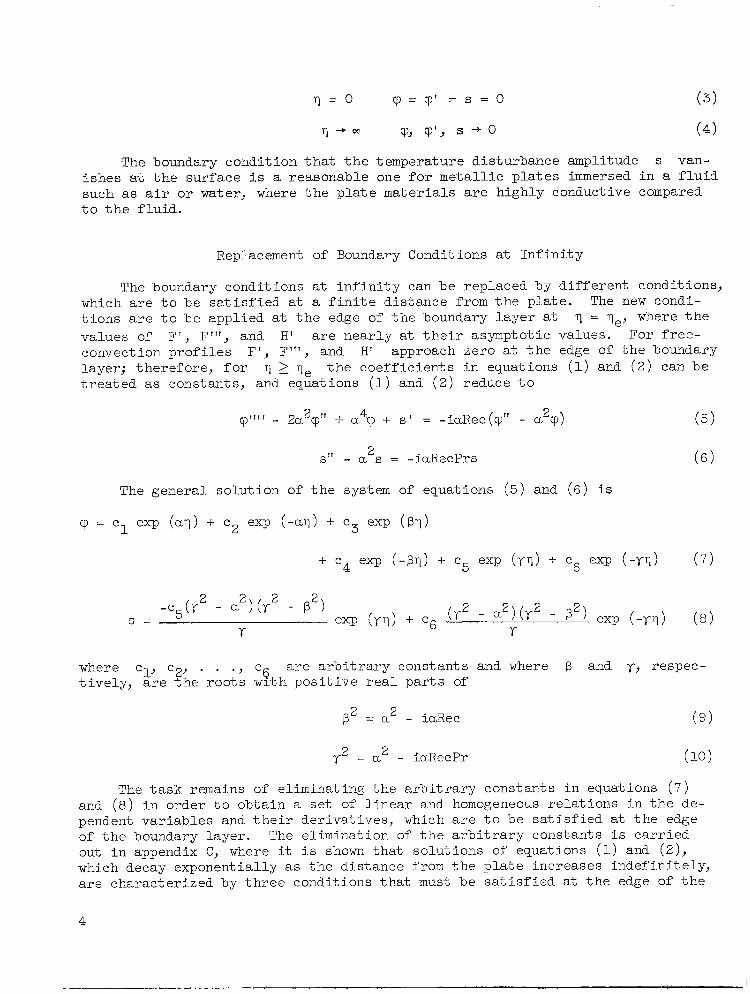
Replacement of Boundary Condit ions at I n f i n i t y

The boundary conditions at i n f i n i t y can be replaced by d i f f e ren t conditions, which a r e t o be s a t i s f i e d a t a f i n i t e d i s tance from t h e plate . The new condi- t i o n s a r e t o be appl ied at t h e edge of t h e boundary l aye r at values of F', F'", and H' a r e near ly a t t h e i r asymptotic values. For free- convection p r o f i l e s F', F"', and HI approach zero at t h e edge of t h e boundary layer; therefore , f o r t r e a t e d as constants, and equations (1) and ( 2 ) reduce t o

71 = ve, where t he

7 2 rle t h e coe f f i c i en t s i n equations (1) and ( 2 ) can be

(5) 2 4 2 cp"" - Z a , cp" + a, cp + s' = -iaRec(cp" - a c p )

(6) 2

S" - a s = -iaRecPrs

The general so lu t ion of t h e system of equations (5) and ( 6 ) is

where el, c2, . . ., c6 a r e a r b i t r a r y constants and where P and y, respec- t i ve ly , a r e t h e roots wi th pos i t i ve real p a r t s of

2 = a' - iaRec

The t a s k remains of e l iminat ing t h e a r b i t r a r y constants i n equations ( 7 ) and (8) i n order t o obtain a s e t of l i n e a r and homogeneous r e l a t ions i n t h e de- pendent var iab les and t h e i r der ivat ives , which are t o be s a t i s f i e d at t h e edge of t h e boundary layer . The elimination of t h e a r b i t r a r y constants i s ca r r i ed out i n appendix C, where it i s shown t h a t so lu t ions of equations (1) and ( 2 ) , which decay exponentially as t h e d is tance from t h e p l a t e increases indef in i te ly , a r e character ized by t h r e e conditions t h a t must be s a t i s f i e d at t h e edge of t h e

4

.... .. . . . . --I

I

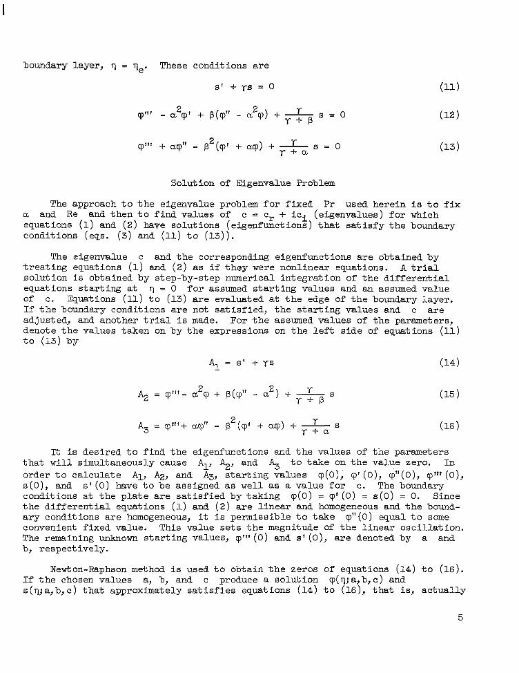
boundary layer, 11 = qe. These conditions a r e

s' + ys = 0

2 2 Cp"' - a cp' + p(cp" - a c p ) + 2 y + p s = O

2 s = o cp"' + q" - p (cp' + up) +

Solution of Eigenvalue Problem

The approach t o t h e eigenvalue problem f o r f ixed Pr used herein i s t o f i x a and R e and then t o f i n d values of c = cr + i c i (eigenvalues) f o r which equations (1) and ( 2 ) have solut ions (eigenfunctions) that s a t i s f y t h e boundary conditions (eqs. (3) and (11) t o (13)).

The eigenvalue c and t h e corresponding eigenfunctions a r e obtained by A t r i a l t r e a t i n g equations (1) and (2) as i f they were nonlinear equations.

so lu t ion i s obtained by step-by-step numerical in tegra t ion of t h e d i f f e r e n t i a l equations s t a r t i n g at 7 = 0 for assumed s t a r t fng values and an assumed value of e. Equations (11) t o (13) a r e evaluated at t h e edge of t h e boundary layer . If t h e boundary conditions a r e not s a t i s f i ed , t h e s t a r t i n g values and c are adjusted, and another t r i a l i s made. For t h e assumed values of t h e parameters, denote t h e values taken on by t h e expressions on the l e f t s ide of equations (11) t o (13) by

A = S ' + YS 1

r s 2 2 % = c p " ' - CL cp + p(cp" - a ) + - r + P

It is desired t o f i n d t h e eigenfunctions and t h e values of t h e parameters t h a t w i l l simultaneously cause Al, %, and t o t a k e on t h e value zero. In order t o ca lcu la te A1, A2, and A3, s t a r t i n g values cp(O), c p ' ( O ) , cp"(O) , cpftf(0), s ( O ) , and s ' ( 0 ) have t o be assigned as wel l as a value f o r e. The boundary conditions ak t h e p l a t e a r e s a t i s f i e d by tak ing Since t h e d i f f e r e n t i a l equations (1) and ( 2 ) a r e l i n e a r and homogeneous and t h e bound- a r y conditions a r e homogeneous, it i s permissible t o t ake cp"(0) equal t o some convenient f ixed value. This value s e t s t h e magnitude of t h e l i n e a r o sc i l l a t ion . The remaining unknown s t a r t i n g values, qff ' (0) and s ' (0), are denoted by a and b, respect ively.

cp(0) = cp'(0) = s(0) = 0.

Newton-Raphson method i s used t o obtain t h e zeros of equations (14) t o (16). If t h e chosen values ay b, and c produce a solut ion cp('q;a,b,c) and s(q;a,b,c) t h a t approximately s a t i s f i e s equations (14) t o (16), that is, ac tua l ly

5

leads t o values of AI, %, and A3 c lose t o zero, then a b e t t e r approximation i s obtained by starting with a + A, b + Ab, and c + Ac instead of a, b, and e, where La, Ab, and Ac a r e obtained as so lu t ions of

Ac (17) z- Ab + ZT aAl A + aa 0 = A1(a,b,c) +

ac F aA2 Ab + aa. ab 0 = A2(a,b,c) +

aA3 ac aA3 Ab + &- ab 0 = A (a,b,c) + 3

The quan t i t i e s A1, %, and A3 and the p a r t i a l der iva t ives evaluated at 7 = ve can be determined by in tegra t ing t h e d i f f e r e n t i a l equations (1) and ( 2 ) by a step-by-step method. be given e i t h e r by a f i n i t e difference approximation or from equations obtained by p a r t i a l d i f f e ren t i a t ion of equations (1) and ( 2 ) with respect t o a, b, and e. (The coe f f i c i en t s of eqs. (1) and ( 2 ) a r e ana ly t i c functions of 7 and depend ana ly t i ca l ly on t h e parameters a, Re, and c. Therefore, t h e solut ions of eqs. (1) and ( 2 ) have t h e same ana ly t i ca l p roper t ies and have t h e required p a r t i a l der ivat ives . ) I n t h e former method four in tegra t ions of equations (1) and ( 2 ) a r e car r ied out, one with a basic s e t a, b, and c, and th ree more, each with appropriate s m a l l increments on a, by and e. P a r t i a l d i f f e ren t i a - t i o n gives t h e same information with one integrat ion. However, i n t h i s second method, t h ree extra s e t s of d i f f e r e n t i a l equations have t o be integrated.

The p a r t i a l der iva t ives i n equations (17 ) t o (19) may

The equations f o r t h e der iva t ives with respect t o a a r e as follows:

(21 ) 2

S" - a s a = iaRePr IF' - c ) sa - 'paH'] a

with t h e i n i t i a l condit ions

The equations f o r t h e der iva t ives with respect t o b a r e a s follows:

(23) - 2a 2 q); + a 4 'pb + s ' = iaRe IF' - c ) ( ' p i - a, 2 'pb) - F1"p]

T' I b

(24) 2 s" b - a sb = iaRePr [F' - c ) s b - ' p b H j

with t h e i n i t i a l conditions

6

and the equations f o r t h e der iva t ives with respect t o c a r e as follows:

with t h e i n i t i a l conditions

In these equations the subscr ipts a, b, and c denote p a r t i a l d i f f e ren t i a - with respect t o a 3 cpl" (0), b = 8 ' ( 0 ) , and c, respectively. For example, (a/aa)(P(q;a,b,c) gives t h e r a t e of change of cp with respect t o a with and -q held constant as a function of q. The p a r t i a l der iva t ives of t h e

At s . appearing i n equations ( 1 7 ) t o (19) can now be evaluated. boundary conditions (eqs. (14) t o (16 ) ) involve c, t h e eigenvalue, through t h e intermediate var iab les /3 and y defined by equations ( 9 ) and (10). Ut i l iz ing equations (14) t o (16) r e s u l t s i n

Note that t h e

s ' 4- ysa aa= a

iaRePr 1 - s 2 r 8' + yg - ac= c

7

I l111111ll11111111l1llII IIIIIIII I I1

aA, 2 r + aq$ - p (% + arpb) + - 'b r + a ab =

For a given point (a,Re) i n t h e a,Re-plane, t h e procedure out l ined should verge t o an eigenvalue e.

Cr i te r ion f o r Convergence t o an Eigenvalue

The procedure out l ined previously f o r f inding t h e eigenvalue f o r a given

The numerical integrat ion point i n t h e a,Re-plane was programed f o r solut ion by using complex ar i thmetic on t h e IBM 7090 located at t h e Lewis Research Center. was done with t h e Runge-Kutta method, which gives fourth-order accuracy. Con- vergence t o an eigenvalue was es tabl ished by requir ing that I All + 1 A21 + 1 A31 < 5x10-6 or requir ing that \AI, 1Ab1, and 1 Acl a l l be l e s s than or equal t o 5X10-6.

2

The s t e p s i z e was externa l ly control led and s e t such t h a t t h e r e was no s ig- n i f i can t change i n t h e eigenvalue when t h e example was rerun with a s t ep s i z e equal t o one-half of t h e o r ig ina l value.

In order t o fix t h e s i z e of t h e solution, t h e eigenfunctions were normalized a f t e r each in tegra t ion so t h a t cp was s e t equal t o u n i t y at t h e edge of t h e boundary layer.

The e f f ec t on t h e r e s u l t s of t h e choice of t h e value of 7 for t h e end of For a i r qe was taken t o be 6, and for t h e range of in tegra t ion was examined.

water qe was taken t o be 5. Variations of ve from these values f o r both cases produced l i t t l e or no changes i n t h e values o f t h e eigenvalues. A s a matter of fac t , qe approximat ions t o t h e eigenvalues.

was taken t o be 3 f o r exploratory runs that resu l ted i n good

Determination of Neutral Curve

The r e s u l t s of t h e s t a b i l i t y analysis a r e usua l ly displayed i n an a,Re- diagram on which t h e curve c i = 0 is drawn. On t h i s curve Re can be consid- ered a funct ion of a. The minimum value of Re for poin ts on t h i s curve i s ca l led t h e minimum c r i t i c a l Reynolds number. The disturbances corresponding t o points i n t h e damped.

u,Re-plane with Reynolds numbers below t h e c r i t i c a l value w i l l be

8

The procedure used herein t o f i n d t h e c r i t i c a l Reynolds number consisted i n holding Re constant and p lo t t i ng t h e imaginary par t c i of t h e establ ished eigenvalues against a. The values of a f o r which c i = 0 could be read from such a graph establ ishing poin ts on t h e neu t r a l curve. For those values of R e below the c r i t i c a l Reynolds number, t h e p lo t of ci against a would not give any c i = 0. However, after t h e c r i t i c a l Reynolds number had been bracketed, a was held constant, and successive l i nea r in te rpola t ions l ed t o t h e c r i t i c a l Reynolds number. Other po in ts on t h e neut ra l curve were obtained by p lo t t i ng c i against e i t h e r a or R e and holding t h e other constant, depending on which choice proved t o be more convenient. Although th i s procedure is s t r a i g h t - forward and easy t o apply, it i s an ind i rec t way t o e s t ab l i sh points on t h e neu t r a l curve. This disadvantage can be a t t r i b u t e d t o t h e choice of t h e complex number c as an eigenvalue. The advantage of using c as an eigenvalue W i l l become apparent after examining the d i f f e r e n t i a l equations t o be integrated.

Fixing a and R e and determining t h e r e l a t i o n between t h e four param- e t e r s t o (13)) correspond t o t h e choice of (cr, c i ) as t h e unknown eigenvalue p a i r and lead t o a system of 24 f i r s t - o r d e r complex d i f f e r e n t i a l equations t o be in te - grated. Since points on t h e neut ra l curve ( c i = 0) are of primary in t e re s t , another choice i s t o s e t among t h e parameters a, Re, and C y by solving equations (17 ) t o (19) with c i = 0 and Aci = 0. Se t t ing c i = 0 leads t o t h e so lu t ion of six real equa- t i o n s i n f i v e real unknowns. In general, th is set of equations w i l l not be con- s i s t e n t unless t h e parameters a, Re, and C y are chosen properly. However, t h e proper value of t hese parameters is t h e information being sought. Since t h e value of c i has been specified, it is no longer permissible t o f i x both a i n order t o provide a consistent set of six real equations i n six real unknowns. However, t h e introduction of t h i s addi t iona l unknown requires t h e in tegra t ion of an addi t iona l set of six f i r s t - o r d e r complex d i f f e r e n t i a l equations.

a, Re, and (cr,ci) by sa t i s fy ing t h e boundary conditions (eqs. (11)

c i = 0 and then attempt t o f i n d t h e proper r e h t i o n

and Re, and t h e va r i a t ion of one of these parameters has t o be allowed f o r

Hence, t h e choice of (cr,c1) as t h e unknown eigenvalue pa i r among t h e pa- rameters t i o n s t o be integrated. This ce r t a in ly j u s t i f i e s t h e choice of c as an eigen- value for t h e case when t h e d i f f e r e n t i a l equations are solved using complex arithmetic. If t h e system of d i f f e r e n t i a l equations is wr i t ten i n real form, t h e number of equations t o b e integrated adds up t o 84. However, 72 of t hese equations involved p a r t i a l der ivat ives with respect t o t h e s t a r t i n g values and t h e eigenvalue c. The number of equations t o be in tegra ted can be reduced i f use is made of t h e property t h a t t h e solut ions of equations (1) and ( 2 ) are ana ly t ic functions of 7 and depend ana ly t i ca l ly on t h e parameters a, Re, and c. This means t h a t the information provided by t h e in tegra t ion of t h e 72 real equations given by equations (20) to (28) can be obtained by the integra- t i o n of only 36 real equations and t h e use of t h e Cauchy-Riemann re la t ions , t hus giving a t o t a l of 48 real equations t o be integrated. change of cp with respect t o ci i s given i n terms of der iva t ives with respect t o cr by r e l a t ions of t h e form: = aqr.cr and a c p r . c i = -acpi/acr. In s i s t i ng that would amount t o r e j ec t ing t h e information furnished by t h e Cauchy-Riemann re la t ions .

a, Re, and (c r ,c i ) leads t o t h e fewest number of d i f f e r e n t i a l equa-

For example, t h e rate of

Act = 0

9

Another j u s t i f i c a t i o n f o r the choice of ( C j c i ) 88 t h e unknown eigenvalue pair , thereby allowing c i t o t ake on nonzero values, is that this choice may lead t o a so lu t ion of the eigenvalue problem, whereas s e t t i n g ci = 0 at t h e outset may eliminate any solutions. case of plane Couette flow has no so lu t ion f o r

For example, t h e eigenvalue problem i n t h e c i = 0.

ENERGY BALANCE O F DISTURBANCE MOTION

After t h e eigenvalue problem has been solved and t h e eigenfunctions have been determined, t h e energy balance of t h e disturbance motion can be computed.

The time rate of increase of t h e disturbance k i n e t i c energy per un i t of volume of a f l u i d p a r t i c l e that moves with t h e bas ic flow i s

An equation governing t h e t ime rate of increase of t h e k ine t i c energy can be obtained by t h e same technique as used i n reference 8 f o r ordinary boundary layers, that is, by multiplying equation (B6) by 5 and equation (B7) by ?, adding these equations, and using equation (B5) t o simplify. T h i s procedure y ie lds

N

where = @;/ax) - (a';/ay).

O f course, a l l disturbance quan t i t i e s a r e taken t o be r e a l i n t h e energy balance equation (39). - respect t o y from y = 0 t o y = m and with respect t o x over a wavelength A of t h e disturbance i n order t o obtain t h e growth of k ine t ic energy per u n i t of time depth and area. After in tegra t ion t h e second and last terms on t h e r igh t s ide of equation (39) vanish s ince u and ? vanish f o r y = 0 and y = m

and have t h e period A with respect t o x. The equation governing t h e time r a t e of increase of k i n e t i c energy of t h e disturbance motion i s

The terms i n t h i s equation a r e t o be integrated with

r u

-

10

The first term i n t h e integrand of t h e r igh t s ide of equation (40) gives t h e '

r a t e at which t h e basic flow, i n v i r t u e of i t s shearing motion, i s working against t h e Reynolds s t r e s s e s a r i s ing frm t h e disturbance, t h e last term repre- sen ts t h e d iss ipa t ion of t h e disturbance motion, and t h e second term represents t h e work done by t h e buoyancy force.

The reference quan t i t i e s introduced i n appendix B a r e used t o transform equation (40) t o t h e following dimensionless form:

where

The disturbance quan t i t i e s i n t h e integrand on t h e r igh t s ide of equa- t i o n (41) a r e given by t h e following re la t ions :

*

N

AT t = a(s(q) exp b u ( ~ - (45)

where R e denotes t h e r e a l par t of t h e complex quantity.

The in tegra ls appearing i n equation (41) a r e evaluated through subs t i tu t ion of equations (43) t o (45) followed by in tegra t ion with respect t o 5 . It is found tha t , f o r neu t r a l disturbances,

The following designations are used t o i den t i fy t h e integrands i n equation (46) :

, , . ... .. .. . ,

e Re = -(cp;cp, -

For neu t ra l disturbances t h e energy balance gives

The s a t i s f a c t i o n of equation (50) provides a check on t h e so lu t ion of t h e eigen- value problem.

BASIC VEmCITY AND TEMPERATLTRE PROFILES FOR WATER

The P r = 0.733 ve loc i ty and temperature p r o f i l e s a r e tabula ted i n r e fe r - ence 9. However, f o r t h e case Pr = 6.7 r e s u l t s were not ava i lab le . In order t o obtain t h e Pr = 6.7 ve loc i ty and temperature prof i les , t h e free-convection boundary value problem was solved by t r e a t i n g it as an i n i t i a l value problem as described i n t h e INTRODUCTION. However, i n this case t h e r e i s no eigenvalue i n t h e equations, r a t h e r t h e proper s t a r t i n g values have t o be determined i n order t o s a t i s f y conditions at i n f i n i t y . The boundary value problem as given i n r e f e r - ence 9 cons i s t s of solving

(51) 2 F"' + 3FF" - 2 ( F ' ) + H = 0

H" -k 3PrFH' = 0 (52)

subject t o t h e boundary conditions

F(0) = F ' ( 0 ) = 0 H(0) = 1 (53)

F ' ( m ) = H ( m ) = 0 (54)

The tabula t ion of t h e Pr = 6 . 7 v e l o c i t y p r o f i l e i s given i n t a b l e I and i s shown i n f igu re 1 along with t h e Pr = 0.733 p ro f i l e .

With t h e ve loc i ty and temperature p r o f i l e s f o r both a i r and water avai lable , t h e s t a b i l i t y of t hese two free-convection boundary-layer flows can be inves t i - gated.

RESULTS AND DISCUSSION

S t a b i l i t y ca lcu la t ions were ca r r i ed out f o r t h e f r e e convection of a i r

12

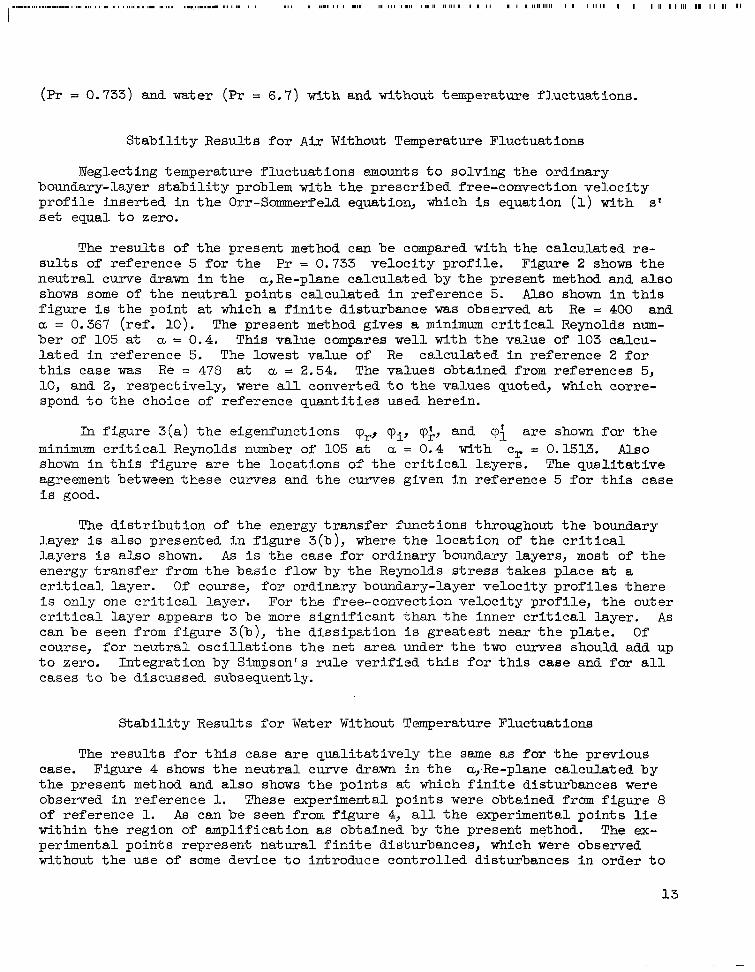
(Pr = 0.733) and water (Pr = 6.7) with and without temperature f luc tua t ions .

S t a b i l i t y Results f o r Air Without Temperature Fluctuations

Neglecting temperature f luc tua t ions amounts t o solving t h e ordinary boundary-layer s t a b i l i t y problem with t h e prescribed free-convection ve loc i ty p r o f i l e inser ted i n the Orr-Sommerfeld equation, which is equation (1) with set equal t o zero.

s f

The r e s u l t s of t h e present method can be compared with t h e calculated re- su l t s of reference 5 f o r t h e Pr = 0.733 ve loc i ty p ro f i l e . Figure 2 shows t h e neutral curve drawn i n t h e a,Re-plane calculated by the present method and a l s o shows some of t h e neu t r a l points calculated In reference 5. D o shown i n t h i s f i gu re i s t h e point at which a f i n i t e disturbance was observed at Re = 400 and a = 0.367 (ref. 10). The present method gives a minimum c r i t i c a l Reynolds num- b e r of 105 at a = 0.4. T h i s value compares w e l l with t h e value of 103 calcu- l a t e d i n reference 5. The lowest value of Re calculated i n reference 2 f o r this case was Re = 478 at a = 2.54. The values obtained from references 5, 10, and 2, respectively, were a l l converted t o t h e values quoted, which corre- spond t o t h e choice of reference quan t i t i e s used herein.

In f igu re 3(a) t h e eigenfunctions (pry (pi, (p;, and 'pi a r e shown f o r t h e minhum c r i t i c a l Reynolds number of 105 at a = 0.4 with cr = 0.1513. Also shown i n t h i s f i gu re a r e t h e locat ions of t h e c r i t i c a l layers . The q u a l i t a t i v e agreement between these curves and t h e curves given i n reference 5 f o r t h i s case i s good.

The d i s t r ibu t ion of t h e energy t r a n s f e r functions throughout t h e boundary layer is a l so presented i n f igu re 3(b) , where t h e loca t ion of the c r i t i c a l l ayers i s a l s o shown. As i s t h e case f o r ordinary boundary layers, most of t h e energy t r a n s f e r from t h e bas ic flow by t h e Reynolds stress takes place at a c r i t i c a l layer. Of course, f o r ordinary boundary-layer ve loc i ty p r o f i l e s t h e r e i s only one c r i t i c a l layer . For t h e free-convection ve loc i ty prof i le , t h e outer c r i t i c a l l ayer appears t o be more s ign i f i can t than t h e inner c r l t i c a l layer. As can be seen f rom f igu re 3(b), t h e dfssfpat ion i s g rea t e s t near t h e p la te . course, f o r neu t r a l o sc i l l a t ions t h e net a r ea under t h e two c m e s should add up t o zero. Integrat ion by Simpson's rule v e r i f i e d this f o r t h i s case and f o r a l l cases t o be discussed subsequently.

O f

S t a b i l i t y Results f o r Water Without Temperature Fluctuations

The r e s u l t s f o r this case are q u a l i t a t i v e l y t h e same as f o r t h e previous case. a,.Re-plane calculated by t h e present method and a l s o shows t h e points at which f in i te disturbances w e r e observed i n reference 1. of reference 1. As can be seen from f igu re 4, a l l t h e experimental po in ts l i e within t h e region of amplif icat ion as obtained by t h e present method. The ex- perimental points represent na tu ra l f i n i t e disturbances, which were observed without t h e Use of some device t o introduce control led disturbances i n order t o

Figure 4 shows t h e neu t r a l curve drawn i n t h e

These experimental po in ts w e r e obtained from f i g u r e 8

13

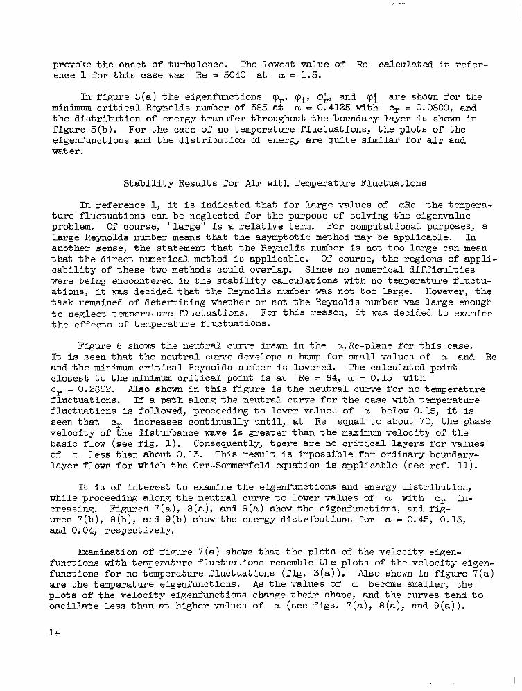
provoke t h e onset of turbulence. The lowest value of R e calculated i n refer- ence 1 f o r t h i s case was R e = 5040 at a = 1.5.

In f igure 5(a) t h e eigenfunctions rp,, Vi, cp;, and cpl are shown f o r t h e minimum c r i t i c a l Reynolds nmber of 385 at a = 0.4125 with C y = 0.0800, and the d i s t r ibu t ion of energy t r a n s f e r throughout t h e boundary layer i s shown i n f igu re 5(b) . For t h e case of no temperature f luctuat ions, t h e p l o t s of t h e eigenfunctions and t h e d i s t r i b u t i o n of energy are q u i t e s imi la r f o r air and w a t er .

S t a b i l i t y Results f o r Air With Temperature Fluctuations

In reference 1, it i s indicated that f o r l a rge values of &e the tempera- t u r e f luc tua t ions can be neglected f o r t h e purpose of solving t h e eigenvalue problem. O f course, "large" i s a r e l a t i v e term. For computational purposes, a l a rge Reynolds number means that t h e asymptotic method may be applicable. another sense, t h e statement that t h e Reynolds number i s not t o o l a rge can mean that t h e d i r e c t numerical method i s applicable. Of course, t h e regions of appl i - c a b i l i t y of these two methods could overlap. w e r e being encountered i n t h e s t a b i l i t y ca lcu la t ions with no temperature f luc tu- ations, it was decided that t h e Reynolds number was not t oo large. However, t h e t a s k remained of determining whether o r not t h e Reynolds number was la rge enough t o neglect temperature f luc tua t ions . For t h i s reason, it w a s decided t o examine t h e e f f ec t s of temperature f luctuat ions.

In

Since no numerical d i f f i c u l t i e s

Figure 6 shows the neu t r a l curve drawn i n t h e a,Re-plane f o r t h i s case. It i s seen t h a t t h e neu t r a l curve develops a hump f o r s m a l l values o f a and R e and t h e minhum c r i t i c a l Reynolds number i s lowered. c loses t t o t h e minimum c r i t i c a l point i s at R e = 64, a = 0.15 with cr = 0.2692. f luctuat ions. f luc tua t ions is followed, proceeding t o lower values of a. below 0.15, it i s seen that cr increases cont inual ly un t i l , at Re equal t o about 70, t h e phase ve loc i ty of t h e disturbance wave is grea te r t han the m a x i " ve loc i ty of t h e basic flow (see f i g . 1). of a less than about 0.13. This r e s u l t i s impossible f o r ordinary boundary- l aye r flows f o r which t h e Orr-Somerf'eld equation is appl icable ( see ref. 11).

The calculated point

Also shown i n this f igure i s t h e n e u t r a l curve f o r no temperature If a pa th along t h e neu t r a l curve f o r t h e case with temperature

Consequently, t h e r e a r e no c r i t i c a l layers f o r values

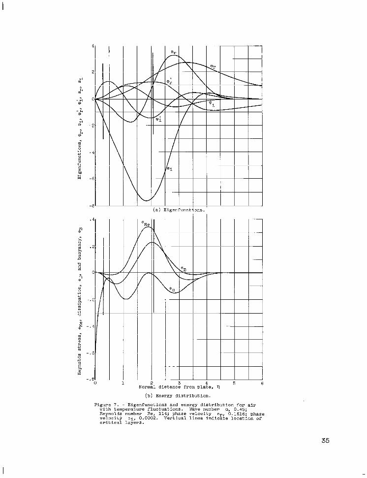
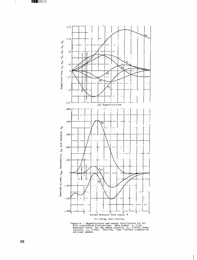
It is of i n t e r e s t t o examine t h e eigenfunctions and energy d is t r ibu t ion , while proceeding along t h e neu t r a l curve t o lower values of a with cr in- creasing. Figures 7 ( a ) , 8(a), and 9 ( a ) show t h e eigenfunctions, and f i g - ures 7(b), 8 (b) , and 9 (b ) show t h e energy d i s t r ibu t ions f o r a = 0.45, 0.15, and 0.04, respectively.

Examination of f igu re 7(a) shows tha t the p l o t s of t h e ve loc i ty eigen- f'unctions with temperature f luc tua t ions resemble t h e p l o t s of t h e ve loc i ty eigen- functions f o r no temperature f luc tua t ions ( f ig . 3 (a ) ) . Also shown i n f igu re 7 ( a ) a r e t h e temperature eigenfunctions. A s t h e values of a become smaller, t h e p l o t s of t h e ve loc i ty eigenfunctions change t h e i r shape, and t h e curves tend t o o s c i l l a t e l e s s than at higher values of a (see f i g s . 7 (a ) , 8(a), and 9 ( a ) ) .

14

Ekamination of t h e energy d i s t r ibu t ions f o r a = 0.45 ( f ig . 7 ( b ) ) shows that the outer c r i t i c a l l ayer i s s igni f icant i n that t h e peak of t h e Reynolds stress-term curve i s located near it, as is t h e case without temperature f luc tu- a t ions. It can be seen that t h e energy d i s t r ibu t ion i s qua l i t a t ive ly the same as fo r no temperature f luctuat ions, except that t h e temperature f luc tua t ion term i s reinforcing t h e Reynolds stress term.

When t h e two c r i t i c a l l ayers are almost coincident at u = 0.15, it i s seen i n f i g u r e 8(b) t h a t the c r i t i c a l l ayers have no cor re la t ion with the energy peak but t h e buoyancy term i s giving a pos i t i ve contribution as i n t h e previous case. Nott that i n t h i s case t h e Reynolds s t r e s s term is not adding energy t o t h e d i s - turbance flow, but is a c t u a l l y subtract ing energy from it. When t h e c r i t i c a l l ayer has completely disappeared as i n f igu re 9(b), it is seen that the buoyancy term i s s t i l l adding energy t o t h e disturbance flow, and again t h e Reynolds stress term i s subtracting.

From t h e previous results it appears that the neglect of temperature f luc tu- a t ions f o r t h e purpose of solving t h e eigenvalue problem can be j u s t i f i e d i n t h e v i c i n i t y of a = 0.35 t o 0.55, where t h e eigenvalues f o r t h e case without tem- perature f luc tua t ions a r e c lose t o t h e eigenvalues f o r t h i s case. However, as can be seen from f igu re 7 (a ) , t h e temperature f luc tua t ions are not negl ig ib le even i n t h i s range of a.

For values of a smaller than a = 0.35, t h e buoyancy term i n t h e energy balance is s igni f icant i n that it is t h e only term t h a t i s giving a pos i t ive contr ibut ion t o t h e energy of t h e disturbance motion, For a = 0.15 and 0.04 it can be seen that t h e Reynolds s t r e s s term i s ac tua l ly extract ing energy. It appears t h a t t h e introduct ion of temperature f luc tua t ions introduces a new mode of i n s t a b l l i t y . This new mode i s characterized by t h e buoyancy force term i n t h e energy balance assuming a dominant role . The buoyancy folrce term is inde- pendent of any property of t h e bas ic flow ve loc i ty p r o f i l e and i s proportional t o t h e g rav i t a t iona l accelerat ion.

The presence of buoyancy e f f e c t s allows the phase ve loc i ty of t h e dis turb- ance wave t o be grea te r than t h e maximum ve loc i ty of t h e bas ic f l o w . problems of hydrodynamic s t a b i l i t y where t h e energy supply t o t h e disturbance i s proport ional t o t h e g rav i t a t iona l force, t h e phase ve loc i ty is grea te r than t h e maximum ve loc i ty of t h e bas ic flow. In fac t , i n reference 1 2 it i s shown, f o r s m a l l wave numbers, that t h e phase ve loc i ty i s equal t o twice t h e maximum veloc- i t y f o r h i n a r flow down an incl ined plane.

In other

S t a b i l i t y Results f o r Water WTth Temperature Fluctuations

The amount of information obtained f o r t h i s case is s ign i f i can t ly less than f o r t h e previous case of air with temperature f luctuat ions, because numerical d i f f i c u l t i e s w e r e encountered for l a rge values of a and Re. Figure 10 shows the neu t r a l curve drawn i n t h e u,Re-plane. A l l t h e points on this curve repre- sent eigenvalues which have the property t h a t the phase ve loc i ty of t h e dis turb- ance wave i s grea te r than t h e m a x i ” ve loc i ty of t h e bas i c flow. ( f ig . 6 ) this property was obtained only for Also shown i n f igu re 10

For a i r cc < 0.13.

15

11111llIIIIlIIIIlII Ill II Ill I I

i s t h e neu t r a l curve f o r water without temperature f luc tua t ions . c u l t t o t r a c e t h e curve with temperature f luc tua t ions f o r higher values of a than shown, because t h e values of t h e eigenfunctions at t h e edge of t h e boundary l aye r changed markedly with each run even though t h e eigenvalues and s t a r t i n g values were only changing i n t h e eighth decimal place. However, even though t h e numerical method cannot produce t h e eigenfunctions, the eigenvalues s o obtained can be accepted as being r e l i a b l e (see ref. 7) . The point at a. = 0.75 and Re = 385 i n f igu re 10 is one where eigenvalues, but not t h e eigenfunctions, can be obtained. This point is on a neu t r a l curve with phase ve loc i ty = 0.1241, which i s l e s s than the maximum ve loc i ty i n t h e bas ic flow (see f i g . :y.

It was d i f f i -

The eigenfunctions f o r R e = 34 at a = 0.45 with cr = 0.1556 a r e shown i n figure l l (a ) , and t h e energy d i s t r ibu t ion f o r t h i s case is shown i n f i g - ure l l ( b ) . It can be seen that t h e two cases, air and water, with temperature f luc tua t ions a r e q u a l i t a t i v e l y t h e same i n that t h e buoyancy term i s providing most of t h e energy input i n t o t h e disturbance motion when the phase ve loc i ty i s g rea t e r than t h e m a x i m u m ve loc i ty i n t h e boundary layer.

CONCLUDING REMARKS

The d i r e c t numerical method gives a minimum c r i t i c a l Reynolds number lower than t h e Reynolds number at which f i n i t e disturbances were observed experimen- t a l l y , whereas calculat ions based on asymptotic techniques y ie ld a minimum c r i t i c a l Reynolds number higher than t h e Reynolds number at which f i n i t e dis- turbances were observed. However, t h e d i r ec t method is not un iversa l ly appl i - cable t o a l l problems for a l l ranges of t h e parameters, espec ia l ly when t h e Reynolds number i s large. Generally, the method should give r e s u l t s i n t h e lower l e f t corner of the i s usua l ly found.

a,Re-plane where t h e minimum c r i t i c a l Reynolds number

By re fer r ing t o t h e r e s u l t s of experiments w i t h na tu ra l disturbances, t h a t is, experiments conducted without t h e use of control led disturbances t o provoke t h e onset of turbulence, it can be concluded that t h e minimum c r i t i c a l Reynolds number calculated herein f o r t h e two cases without temperature f luc tua t ions pro- vides a lower bound t o t h e Reynolds number at which f i n i t e disturbances were ob- served. However, inclusion of temperature f luc tua t ions indicated t h a t t h i s mini- mum c r i t i c a l Reynolds number is not the least lower bound. Rather, t h e r e i s a lower m'lnimum c r i t i c a l Reynolds number at s m a l l values of Wave number a. This in s t ab i l i t y , f o r which t h e phase ve loc i ty of t h e disturbance wave i s g rea t e r than t h e maximum ve loc i ty of the bas ic flow i n t h e boundary layer, has not been re- ported i n t h e accounts of na tura l t r a n s i t i o n experiments.

The existence of temperature f luc tua t ions provides a new mechanism of energy t r a n s f e r t o t h e k ine t i c energy of t h e disturbance motion. This amount of energy is a s ign i f i can t contribution t o t h e energy balance i n that, for a l l cases calculated, it w a s always posi t ive, t h a t is, des tab i l iz ing .

Lewis Research Center National Aeronautics and Space Administrat ion

Cleveland, Ohio, September 19, 1963

I

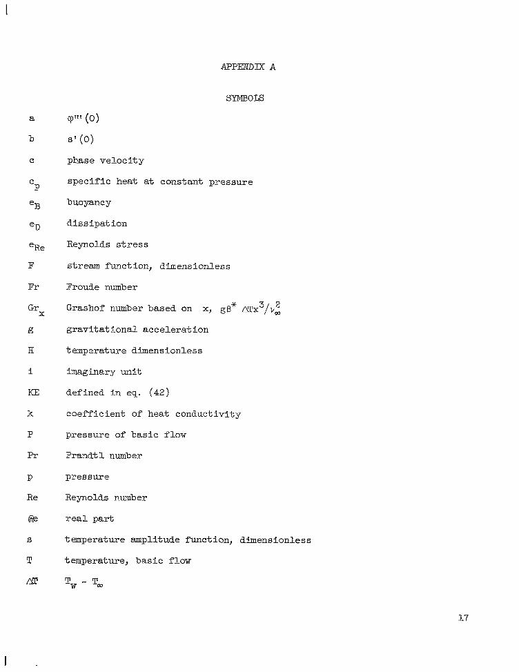
a

b

C

C P

eB

eD

eRe

F

Fr

G r

l3

H

i

m

k

P

Pr

P

Re

6?e

X

S

T

m

s p e c i f i c heat at constant pressure

buoyancy

d i s s ipa t ion

Reynolds stress

stream function, dimensionless

Froude number

Grashof number based on

g rav i t a t iona l acce lera t ion

x, gp* ECx 3 2 /v,

temperature dimensionless

imaginary uni t

defined i n eq. (42)

coef f ic ien t of heat conductivity

pressure of bas ic flow

Prandt 1 number

pressure

Reynolds number

r e a l pa r t

temperature amplitude f'unct ion, dimensionless

temperature, bas ic flow

Tw - Tco

17

I

wall temperature

ambient t emp erat ure

t emp eratur e

v e l o c i t y p a r a l l e l t o plate , bas ic flow

reference ve loc i ty p a r a l l e l to p l a t e

ve loc i ty p a r a l l e l to p l a t e

v e l o c i t y normal to plate, bas ic flow

ve loc i ty normal to p l a t e

d is tance from leading edge of p l a t e

normal d is tance from p l a t e

wave number

coef f ic ien t of volumetric expansion

reference length, -@x/ ( G r x ) 1/4

normal d is tance from plate , dimensionless

edge of boundary layer

wavelength, Zx/a, dimensionless

coef f ic ien t of v i scos i ty

kinematic v i s c o s i t y

dis tance from leading edge of plate , dimensionless

dens i ty

time, dimensionless

stream funct ion amplitude, dimensionless

stream function, dimensionless

Subscript s :

a, b, c

i r e f e r s to imaginary pak-t

denotes d i f f e r e n t i a t i o n with respect to quant i ty

18

m a x m a x i "

r r e fe r s t o r e a l par t

Superscripts:

N disturbance quant i ty

- dimensional quant i ty

I d i f f e ren t i a t ion with respect t o 7

19

.. ..... ,.,.. I,.. I I..

DERIVATION OF STABILITY EQUATIONS

The governing equations f o r a p a r a l l e l bas i c f low plus a disturbance as given i n reference 1 a r e as follows:

au + av = G a y

where

+=a+- a 2 ax2 ay2

The bas ic s teady-s ta te flow i s t h e free-convection flow about a v e r t i c a l heated p la te . has been neglected except i n t h e g rav i ty term where t h e dens i ty was taken t o de- pend l i n e a r l y on t h e temperature. I n equations (B1) t o (B4) t h e density, where it appears, i s taken t o be a constant. I n accordance with t h e paral le l - f low assumption, t h e bas ic flow can be described by T = T(y) . Superimposed upon t h e basic flow i s a two-dimensional disturbance. The disturbance equations a r e obtained by subs t i t u t ing p = P + G, and t = T + flow, and neglecting products of disturbance quan t i t i e s and t h e i r der ivat ives . The disturbance equations a r e

In t h e der iva t ion of t h e governing equations t h e va r i a t ion of t h e dens i ty

U = U(y), V = 0, P = P(y), and

u = U + u, v = ?, N

i n t h e previous equations, subtract ing out t h e bas ic

-. . . - -- . . . . . . .

20

The disturbance v e l o c i t i e s can be obtained from a stream funct ion

from which

As can be seen from equation (B9), t h e disturbance i s taken t o be per iodic i n t h e d is tance x along t h e p la te . The pos i t i ve quant i ty E i s t h e wave num- ber of a disturbance wave, and Fr, t h e real par t of F, is t h e ve loc i ty of propagation of t h e wave. The imaginary pa r t of S w i l l determine whether t h e disturbance w i l l grow (Ci > 0) o r decay (Fi < 0) i n time. turbance i s a l s o per iodic i n t h e dis tance x along t h e p l a t e and may be ex- pressed as

The temperature dis-

It is convenient t o represent t h e disturbance quan t i t i e s i n complex form in order t o s a t i s f y t h e phase r e l a t ions imposed by equations (E) t o (B8). However, physical s ign i f icance i s t o be at tached only t o t h e r e a l par t of disturbance quant i t ies .

Dimensionless var iab les a r e introduced by choosing reference quan t i t i e s i n conformity with those used i n ca lcu la t ing t h e bas ic flow as follows:

Length:

Velocity:

X

Temperature :

where

Tw - T, E A!T

Gr = gp* m x 3 X 2

v,

21

lllIlIlIlII1111IIIl II I I 1 I

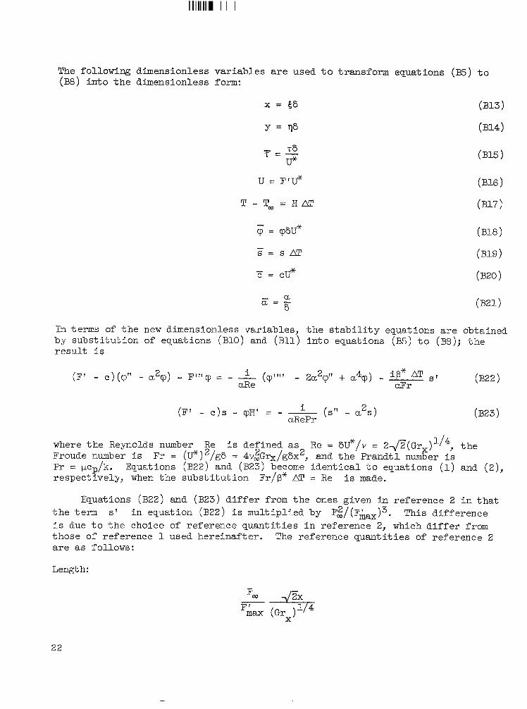
The following dimensionless var iab les are used t o transform equations (B8) i n t o t h e dimensionless form:

(E) ' to

- cp = cpFU* - s = s m

c = cu - *

In terms of t h e new dimensionless var iables , t h e s t a b i l i t y equations a r e obtained by subs t i t u t ion of equations (B10) and (B11) i n t o equations (B5) t o (B8); t h e r e s u l t i s

2 (SI' - a s ) i (F' - c ) s - cpR' = - -

aRePr

where t h e Reynolds number Re i s defined as Re = 6U*/v = 2fi(Grx)1/4, t h e Froude number i s Pr = pcp/k. respectively, when t h e subs t i t u t ion Fr/B* AT = Re i s made.

Fr = ( p ) 2 / g S = 4v2Grx /gSx 2 , and t h e Prandt l number i s Equations (B22) and (B23) become i d e n t i c a l t o equations (1) and ( 2 ) ,

Equations (B22) and (B23) d i f f e r from t h e ones given in reference 2 i n t h a t t h e term s ' i n equation (B22) i s mult ipl ied by F$/(Fhax)3. This difference i s due t o t h e choice of reference quan t i t i e s i n reference 2, which d i f f e r from those of reference 1 used hereinaf ter . The reference quan t i t i e s of reference 2 a r e as follows:

Len& h :

X

2 2

Velocity:

23

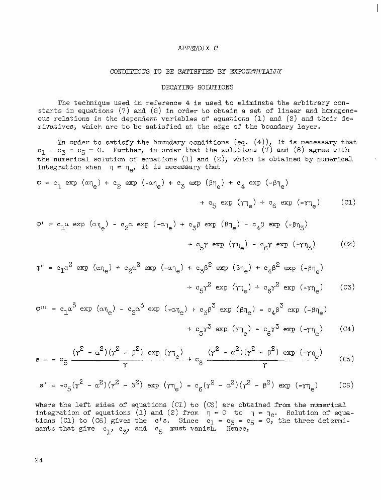
APPENDIX c

commroxs TO BE SATISFIED BY EXPONENTIALLY

DECAYING SOLUTIONS

The technique used i n reference 4 i s used t o eliminate t h e a r b i t r a r y con- s t a n t s i n equations ( 7 ) and (8) i n order t o obtain a s e t of l i n e a r and homogene- ous r e l a t ions i n the dependent var iab les of equations (1) and (2 ) and t h e i r de- r iva t ives , which a r e t o be s a t i s f i e d a t t h e edge of t h e boundary layer .

In order t o s a t i s f y t h e boundary conditions (eq. (4)), it is necessary t h a t c1 = c3 = c5 = 0. Further, i n order that t h e solut ions ( 7 ) and (8) agree with t h e numerical solut ion of equations (1) and ( Z ) , which i s obtained by numerical in tegra t ion when 7 = ve, it i s necessary tha t

where t h e l e f t s ides of equations (Cl) t o ( C 6 ) a r e obtained from t h e numerical in tegra t ion of equations (1) and ( 2 ) from 7 = 0 t o 7 = qe. Solution of equa- t i o n s ( C l ) t o ( C 6 ) gives t h e e ' s . Since nant s t h a t give

c1 = c3 = c5 = 0, t h e th ree determi- cl, c3, and c must vanish. Hence, 5

24

1 1 1 1 cp 1

a -a p - p cp' -.Y-

2 a2 a2 p2 p2 cp" Y

a -a p3 - p c p l ' l -Y 3 3 3 3

1 1 1 1 cp 1

a -a p - p cp' -Y-

2 a2 a2 p2 p2 cp" Y = o = o

Equations ( C 7 ) t o ( C 9 ) reduce to

= 0 (c7)

= 0 ( C 8 )

25

5' + ys = 0 ( c12 1 Equations (C10) t o ((212) a r e the conditions that the numerical so lu t ion m u s t sat- i s f y a t t h e edge of t h e boundary l aye r at It is convenient t o eliminate s' from equations ( C 1 0 ) and (C11) by means of equation (C12). This leads t o the somewhat simpler conditions t h a t w i l l be employed instead of equations (Cll) and (ClO), respectively, namely,

q = qe.

s = o 2 2 q'" - a, cp' + p(cp" - a c p ) + L r + P

s = o qf" + ucp" - p 2 (9' - acp) + T+a

It is c lea r that, i f equations ( C 1 2 ) t o (C14) a r e satisfied, then so a r e equa- t i o n s (C10) and ((211).

26

REFERENCES

1. Szewczyk, Albin A. : S t a b i l i t y and Transi t ion of t h e Free-Convection Layer Along a Ver t i ca l F l a t Plate . In t . Jour. of Heat and Mass Transfer, vol. 5, 1962, pp. 903-914.

2. Plapp, J. E.: I. Laminar Boundary Layer S t a b i l i t y i n Free Convection. 11. Laminar Free Convection with Variable Fluid Propert ies . Ph.D. Thesis, C. I. T., 1957.

3. Brown, W, Byron, and Sayre, Ph i l ip H.: An Exact Solution of t h e O r r - Sommerf e ld S t a b i l i t y Equation f o r Low Reynolds Numbers. Rep. BLC-43, Northrop Aircraft , Inc., May 1954.

4. Brown, W. B.: A S t a b i l i t y Cr i te r ion f o r Three-Dimensional Laminar Boundary Layers. Boundary Layer and Flow Control, vol. 2, G. V. Lachmann, ed., Pergamon Press, 1961, pp. 913-923.

5. Kurtz, Edward Fulton, Jr.: A Study of t h e S t a b i l i t y of Laminar P a r a l l e l Flows. Ph.D. Thesis, M.I.T., 1961.

6. Thomas, L. H.: The S t a b i l i t y of Plane Po i seu i l l e Flow. Phys. Rev., vol. 86, no. 5, June 1952, pp. 812-813.

7. Fox, Leslie: Some Numerical Experiments with Eigenvalue Problems i n Ordinary Di f f e ren t i a l Equations. Boundary Problems i n Di f f e ren t i a l Equations, R. E. Langer, ed., The Univ. of Wisconsin Press, 1960, pp. 243-255.

8. Schlichting, H.: Amplitude Dis t r ibu t ion and Energy Balance of Small D i s - turbances i n P l a t e Flow. NACA TM 1265, 1950.

9. Ostrach, Simon: An Analysis of Laminar Free-Convection Flow and Heat Trans- f e r About a F l a t P l a t e P a r a l l e l t o t h e Direction of t h e Generating Body Force. NACA Rep. 1111, 1953. (Supersedes NACA T N 2635. )

10. Eckert, E. R. G., S'dhngen, E., und Schneider, P. J.: Studien zum Lhschlag laminar-turbulent der f r e i e n Konvektions-Str'cjmung an e iner seckrechten P l a t t e . 50 Jahre Grenzschichtforschung, Fr iedr . Vieweg & Sohn, Braunschweig, 1955, pp. 407-418.

11. Koppel, Donald H . : Review of Three Classic Problems i n Hydrodynamic S tab i l - i t y . Tech. Rep. 86, Hudson Labs., Columbia Univ., Feb. 15, 1960, pp. 15-18.

12. Benjamin, T. Brooke: Wave Formation i n Laminar Flow Down an Incl ined Plane. Jour. F lu id Mech., p t . 6, vol. 2, Aug. 1957, pp. 554-574.

27

TABLE I. - FUNCTIONS F AND H AND DERIVATIVES

FOR P R A " NUMBER OF 6.7

H

1.0000 .e700 -7412 -6162 -4986

.3919 -2989 -2212 .1588

.1107

.0751 -0496 .0319

.0201 ,0124 .0075 -0044

-002 6 .0015 .0008 .0005

.0003

. O O O l

. O O O l . 0000

.oooo

.oooo

.oooo . 0000

.oooo

.oooo

.oooo

.oooo

.oooo .oooo .oooo .oooo

.OOOO' . 0000 . 0000 . 0000

.oooo

.oooo

71 0.

.125C -250C .375c .500C

.625C

.7SOC

.875C 1. oooc 1.125C 1.250C 1.3750 1.500C

1.6250 1.7500 1.8750 2.0000

2.1250 2.2500 2.3750 2.5000

2.6250 2.7500 2.8750 3.0000

3.1250 3.2500 3.3750 3.5000

3.6250 3.7500 3.8750 4.0000

4.1250 4.2500 4.3750 4.5000

4.6250 4.7500 4.8750 5.0000

5.1250 5.2500 5.3750 5.5000

5.6250 5.7500 5.8750 6.0000

6.1250 6.2500 6.3750 6.5000

6.6250 6.7500 6.8750 7.0000

7.1250 7 -2500 7.3750 7.5000

8.1250 .2777

I8.375oI 8.2500 .2778 .27781

,2774 .2775

18.50001 -27781

.oooo

.oooo

.oooo

.oooo . 0000 . 0000

.oooo . 0000

.oooo

.oooo

.oooo

.oooo

.oooo

.oooo

.oooo . 0000

.oooo f 0000

.oooo . 0000 . 0000

.oooo

.oooo

.oooo * 0000 .oooo

-.

F -~ ). -003: .011€ .0241 .038€

.054€

.071E

.088C -1041

.1194

.133E ,147: .159:

.1707 -181C .1904 .1986

.206E

.213E

.22oc

.2257

.2309

.2355

.2397

.2436

-2.170 .2501 .2529 .2554

.2577 .2597 -2616 .2633

-2648 .2661 .2673 .2684

.2694 .2703 -2711 .2718

.2725

.2731

.2736

.2741

.2745

.27.19

.2752

.2755

.2758

.2760

.2763

.2765

.2766

.2768

.2769 ,2771

,2772 ,2773

-

F'

1. -049, .085: .lo91 .124,

.13M

.133!

.131:

.125!

,118: .111( .lo21 .094:

.OB62

.078f

.071<

.064€

.058i -0535 .0481 .043E

.039:

.035:

.0321

.0285

.0261

.O23€

.021: -0192

-017: . Ol5f .014C .0127

-0114 .0101 .0092 .0089

.0075

.0068 -0061 -0055

.0049

.0044 .0040 .0036

.0032 ,0029 .002 6 .0023

.0021 -0019 .0017 .0015

.0013

.0012

.0011

.OOlO

.0009 -0008 .0007 ,0006

.0005

.0005

.0004 ,0004

.0003

.0003 ,0002 ,0002

F"

0.454 .337 .237 .154 .086

.034 -. 004 -. 032 -. 050

-. 060' -. 065' -. 067 - .065!

-. 0631 -. 059: -. 055: -. 0501

-. 0461 - .042! - .038' - .035:

- .0311 -.028L -. 026: - .023:

-. 021: -. 0191 -. 017: -. 015:

- .014: - . 012: -. O l l i -. 010: -. 009: -. 008E -. 007; -. 007(

-. 0062 -. 0057 -. 0051 -. 004E

- . 0042 . . 003E . .0034 . .0031

-. 0028 -. 0025 -. 0022 - .002c

-. 0018 -. 0016 . .0015 . .0013

. .0012 -. 0011 -. 0010 . ,0009

. .0008 - .0007 . .0006 . .0006

. .0005

. .0005

. .0004

. .0004

.0003

.0003 ' . 0003 . .0003

F"'

-1.0001 -. 868. -. 735: - .603: -. 477'

-. 3621 -. 262: -.178: -. 111! -. 060' -. 024(

.001:

.017.

.027:

.032: -034: -0341

.033:

.0314

.029:

.0271

.024E

.022€

.020€

.019c

.0172

.0157

.0142

.012E

.0117 . O l O f

.009 E

.OO8f

.007e

.007 1

.0064 -0058

.0052 -0047 -0042 .0038

-0035 .0031 .0028 .0025

.0023

.0021

.0019 -0017

-0015 .0014 .0012 .0011

.OOlO

.0009

.0008

.0007

.0007 ,0006 .0005 .0005

.0004

.0004 -0004 .0003

.0003

.0003 -0002 .0002

H'

1.040, 1.037 1.019 -. 975' -. 901

- . a o i -. 684 -. 559' -. 439

-. 3321 -. 2411 -. 1691 -. 115.

-. 076: -. 049( - ,030' -. 0181

-. 011; - . 006; -. 003: -. 002:

- .001: - . OOOi - . 000' - . 000:

- .0001 - .0001 . oooc . oooc . OOO( . oooc . oooc . oooc . oooc . oooc . oooc . oooc . oooc . oooc . oooc .oooc . oooc . oooc .oooo .oooo .oooo .oooo .oooo .oooo

.oooo . 0000

.oooo . 0000

. 0000

.oooo

.oooo . 0000

. 0000 . 0000 . 0000 . 0000

.oooo

.oooo . 0000 .oooo .oooo .oooo .oooo . 0000

28

I

.28

.24

.20

- .16 h

2 c) rl u 0 rl

.12

.08

.04

0

I

I

F 0.733

\ i

7 u

I -F'randtl-

number, pr

r\ 1 2 3 4 5 6 7

Normal distance from pla te , q

Figure 1. - Velocity p r o f i l e s for two Prandt l numbers.

29

-

w 0

,r-- t------------------~

16%87---

.--

I I I .lL-L-LL-L----

150 390 400 110 120 130 140 100 Reynolds number, R e

Figure 2. - Neutral curve for air without temperature f luctuat ions.

-4 0

- k 0

d e-

R 0

m 5 d .u

$ %l

M d w 8

F1

57 d 42

a d m

d a a d

a, p:

31 4 I I k E 4 I

(a) Eigenfunctions.

'Re

\ \

- '. /

2 3 4 Normal distance from plate, 11

(b) Energy distribution.

Figure 3. - Eigenfunctions and energy distribution f o r air without temperature fluctuations. Wave number a, 0.4; Reynolds number Re, 105; phase velocity cy? 0.1513; phase velocity ci, 0. Vertical lines indicate location of critical layers.

31

d

Calculated points of present method ------ 0 -

----- 560 600 640

-1. 360 - 400 440 480 520

Reynolds number, Re

Figure 4. - Neutral curve for water without temperature fluctuations.

3

2 - 4 e

- & e

$ 1

k e

: o c1 0

3 Q

tu w" -1

-2

.12

. oa

!2

z .04

c,

a d m m

d V

a 0 ld

P) p:

$ -.04 m P) - m a r( -.oa p: i

-.12

- .1E

~

A 1 2 3 Normal d is tance from p l a t e , ll-

(b) Energy d i s t r i b u t i o n .

Figure 5 . - Elgenfunctions and energy d i s t r i b u t i o n for water without temperature f luc tua t ions . Wave number a, 0.4125; Reynolds number Re, 385; phase v e l o c i t y cy, 0.800; phase ve loc i ty c i , 0. Ver- t i c a l l i n e s ind ica t e loca t ion of c r i t i c a l l aye r s .

33

i i I I

Phase velocity,

100

/ /

.

Calculated points of present method - With temperature fluctuations - - - - Without temperature fluctuations

i - - + 12 0 140 160 180 2 00

Reynolds number, Re

Figure 6. - Neutral curve for air with and without temperature fluctuations.

34

(a) Eigenfunctions.

(b) Energy distribution.

Figure 7. - Eigenfunctions and energy distribution f o r air with temperature fluctuations. Wave number a, 0.45; Reynolds number Re, 114; phase velocity cy, 0.1616; phase velocity e l , 0.0002. Vertical lines indicate location of critical layers.

35

ll1111l1ll11l1llI Illllll II IIIIIII

-.- ( a ) Elgenfunctions.

Normal distance

(b) Energy distribution.

Figure 8. - Elgenfunctions and energy distribution for air with temperature fluctuations. Wave number a, 0.15; Reynolds number Re, 64; phase velocity cy, 0.2692; phase velocity Ci, 0.0001. Vertical lines indicate location of critical layers.

36

I

1.2

.8

.4

0

-.4

-030

.020

-01c

C

-. 01c

-. 02c

(a) Eigenfunctions.

'\

N o r m a l distance from plate, q

(b) Energy distribution.

Figure 9. - Eigenfunctions and energy distribution for air with tempera- ture fluctuations. Wave number a, 0.04; Reynolds number Re, 137; phase velocity cr, 0.3414; phase velocity ci, 0.0001.

37

Phase v e l o c i t y , Cr

.8

3-0 .13bO I

d-- /

I - 0 C a l c u l a t e d p o i n t s o f p r e s e n t method I 1 // - With t e m p e r a t u r e f l u c t u a t i o n s . 7

I I _ _ _ Without t e m p e r a t u r e f l u c t u a t i o n s

\ \ I 3

- 0 50 100 150 200 250 300 350 400 450 5 00 550 600

Reynolds number, R e

F i g u r e 10. - N e u t r a l c u r v e f o r water w i t h and w i t h o u t t e m p e r a t u r e f l u c t u a t i o n s .

2

d m

L O

3 9

Lh * -2

d 9

L 9

m' -4

*-' 0 C

i 2 - 6 M irl d

- .4

-IC

1 . k

m @.I

x

m . c 2 0

P

-0 c m

5 .;

c * Y

m e .:

- a

& : m

h u m

2 -.: 2 2

r(

-..

- . f

C t l T I 8.

.ante from plate,

(b) Energy distribution

Figure 11. - Elgenfunctions and energy distrlbution for water with temperature fluctuations. 'Xave number a, 0.45; Reynolds r,,iber Re, 34; phase velocity cy, 0.1556; phase velocity cl, 0.

NASA-Langley, 1963 E-2172 39