stability of fractional-order systems … of fractional-order systems with rational orders: a survey...

STABILITY OF FRACTIONAL-ORDER SYSTEMS

WITH RATIONAL ORDERS: A SURVEY

Ivo Petras

Abstract

In this survey paper we review the methods for stability investigation ofa certain class of fractional order linear and nonlinear systems. The stabilityis investigated in the time domain and the frequency domain. The generalstability conditions and several illustrative examples are presented as well.

Mathematics Subject Classification: 26A33 (main), 93D25, 30F99Key Words and Phrases: fractional calculus, complex plane, stability,

fractional-order system, time domain, frequency domain

1. Introduction

Fractional Calculus (FC) is more than 300 years old topic. A numberof applications where FC has been used rapidly grows, especially duringlast two decades. This mathematical phenomena allow to describe a realobject more accurate that the classical “integer” methods. The real objectsare generally fractional [38, 40, 48, 66, 68], however, for many of them thefractionality is very low. The main reason for using the integer-order modelswas the absence of solution methods for fractional differential equations.

Recently, the fractional order linear time invariant (FOLTI) systemshave attracted lots of attention in control systems society (e.g. [17, 32, 40,50, 52]) even though fractional-order control problems were investigated asearly as 1960s [33]. In the fractional order controller, the fractional order

c© 2009 Diogenes Co. (Bulgaria). All rights reserved.

270 I. Petras

integration or derivative of the output error is used for the current controlforce calculation.

The fractional order calculus plays an important role in physics [43,58, 64], thermodynamics [29, 55], electrical circuits theory and fractances[6, 12, 15, 20, 38, 67], mechatronics systems [53], signal processing [54, 65],chemical mixing [39], chaos theory [60, 63], etc. It is recommended to referto (e.g. [7,37,41,57,69]) for the further engineering applications of fractionalorder systems. The question of stability is very important especially incontrol theory. In the field of fractional-order control systems, there aremany challenging and unsolved problems related to stability theory such asrobust stability, bounded input - bounded output stability, internal stability,root-locus, robust controllability, robust observability, etc.

For distributed parameter systems with a distributed delay [42], pro-vided an stability analysis method which may be used to test the stabilityof fractional order differential equations. In [13], the co-prime factoriza-tion method is used for stability analysis of fractional differential systems.In [34], the stability conditions for commensurate FOLTI system have beenprovided. However, the general robust stability test procedure and proofof the validity for the general type of the FOLTI system is still open anddiscussed in [46]. Stability has also been investigated for fractional ordernonlinear system (chaotic system) with commensurate and incomensurateorder as well [2, 60,61].

This paper is organized as follows. Section 2 is a brief introduction tothe fractional calculus. Section 3 is on fractional order systems. In Section4 the stability conditions of the fractional order systems are described. In-vestigation methods for linear systems are described in Section 5, and fornonlinear systems – in Section 6. Section 7 concludes the paper with someremarks.

2. Fractional calculus fundamentals

The idea of fractional calculus has been known since the development ofthe classical calculus, with the first reference probably being associated withLeibnitz and l’Hospital in 1695 where half-order derivative was mentioned.

Fractional calculus is a generalization of the integration and differentia-tion to non-integer order fundamental operator aD

αt , where a and t are the

limits of the operation and α ∈ R.The three definitions often used for the general fractional differinte-

gral are the Grunwald-Letnikov definition, the Riemann-Liouville and the

STABILITY OF FRACTIONAL-ORDER SYSTEMS . . . 271

Caputo definition, see e.g. [39, 48]. For our purpose we use the Caputo’sdefinition (originated from his 1967’s paper [14]), which can be written as

aDαt f(t) =

1Γ(α− n)

∫ t

a

f (n)(τ)(t− τ)α−n+1

dτ, (1)

for (n−1 < α < n). The initial conditions for the fractional order differentialequations with the Caputo’s derivatives are in the same form as for theinteger-order differential equations.

The formula for the Laplace transform of the Caputo’s fractional deriva-tive (1) for zero initial conditions has the form [48]:

L0Dαt f(t) = sαF (s), (2)

where s ≡ jω denotes the Laplace operator.Geometric and physical interpretation of fractional integration and frac-

tional differentiation was given in Podlubny’s work [49].

3. Fractional-order systems

A general fractional-order linear system can be described by a fractionaldifferential equation of the form

anDαny(t) + an−1Dαn−1y(t) + . . . + a0D

α0y(t)= bmDβmu(t) + bm−1D

βm−1u(t) + . . . + b0Dβ0u(t), (3)

where Dγ ≡ 0Dγt denotes the Riemann-Liouville or Caputo’s fractional

derivative [48], or by the corresponding transfer function of incommensuratereal orders of the following form [48]:

G(s) =bmsβm + . . . + b1s

β1 + b0sβ0

ansαn + . . . + a1sα1 + a0sα0=

Q(sβk)P (sαk)

, (4)

where ak (k = 0, . . . , n), bk (k = 0, . . . , m) are constant, and αk (k =0, . . . , n), βk (k = 0, . . . , m) are arbitrary real or rational numbers andwithout loss of generality they can be arranged as αn > αn−1 > . . . > α0,and βm > βm−1 > . . . > β0.

The incommensurate order system (4) can also be expressed in com-mensurate form by the multivalued transfer function [9]

H(s) =bmsm/v + . . . + b1s

1/v + b0

ansn/v + . . . + a1s1/v + a0, (v > 1). (5)

272 I. Petras

Note that every fractional order system can be expressed in the form (5)and domain of the H(s) definition is a Riemann surface with v Riemannsheets, [30].

In the particular case of commensurate order systems, it holds thatαk = αk, βk = αk, (0 < α < 1), ∀k ∈ Z, and the transfer function has thefollowing form:

G(s) = K0

∑Mk=0 bk(sα)k

∑Nk=0 ak(sα)k

= K0Q(sα)P (sα)

. (6)

With N > M , the function G(s) becomes a proper rational function inthe complex variable sα which can be expanded in partial fractions of thefollowing form:

G(s) = K0

[N∑

i=1

Ai

sα + λi

], (7)

where λi (i = 1, 2, ..., N) are the roots of the pseudo-polynomial P (sα) orthe system poles which are assumed to be simple without loss of generality.

Consider a control function which acts on the FODE system as follows:

an Dαnt y(t) + · · ·+ a1 Dα1

t y(t) + a0 Dα0t y(t) = u(t). (8)

By Laplace transform, we can get a fractional transfer function:

G(s) =Y (s)U(s)

=1

ansαn + · · ·+ a1sα1 + a0sα0. (9)

The analytical solution of the FODE (8) for u(t) = 0 is given by generalformula in the form [48]:

y(t) =1an

∞∑

m=0

(−1)m

m!

∑k0+k1+...+kn−2=m

k0≥0;... ,kn−2≥0

(m; k0, k1, . . . , kn−2)

×n−2∏

i=0

(ai

an

)ki

Em(t,−an−1

an; αn − αn−1, αn

+n−2∑

j=0

(αn−1 − αj)kj + 1), (10)

where (m; k0, k1, . . . , kn−2) are the multinomial coefficients and Ek(t, y;µ, ν)is the function of Mittag-Leffler type introduced by Podlubny [48]. Thefunction is defined by

Ek(t, y; µ, ν) = tµk+ν−1E(k)µ,ν(ytµ), (k = 0, 1, 2, . . .), (11)


where Eµ,ν(z) is the Mittag-Leffler function of two parameters [25]:

Eµ,ν(z) =∞∑

i=0

zi

Γ(µi + ν), (µ > 0, ν > 0), (12)

where e.g. E1,1(z) = ez, and where its k-th derivative is given by

E(k)µ,ν(z) =

∞∑

i=0

(i + k)! zi

i! Γ(µi + µk + ν), (k = 0, 1, 2, ...). (13)

The fractional-order linear time invariant (LTI) system can also be rep-resented by the following state-space model

0Dqt x(t) = Ax(t) + Bu(t)

y(t) = Cx(t), (14)

where x ∈ Rn, u ∈ Rr and y ∈ Rp are the state, input and output vectors ofthe system and A ∈ Rn×n, B ∈ Rn×r, C ∈ Rp×n, and q = [q1, q2, . . . , qn]T

are the fractional orders. If q1 = q2 = . . . = qn ≡ α, system (14) is calleda commensurate order system, otherwise it is an incommensurate ordersystem. If Caputo’s derivative is considered, the initial conditions are:

x1(0) = x(1)0 = y0, x2(0) = x

(2)0 = 0, . . .

xi(0) = x(i)0 =

y

(k)0 , if i = 2k + 1,

0, if i = 2k,i ≤ n. (15)

Similar to conventional observability and controllability concept, thecontrollability is defined as following [36]: System (14) is controllable on[t0, tfinal] if the controllability matrix

Ca = [B|AB|A2B| . . . |An−1B]

has rank n.The observability is defined following [36]: System (14) is observable on

[t0, tfinal] if the observanility matrix

Oa =[

C|CA|CA2| . . . |CAn−1]T

has rank n.

274 I. Petras

Generally, we consider the following incommensurate fractional-ordernonlinear system in the form:

0Dqit xi(t) = fi(x1(t), x2(t), . . . , xn(t), t)xi(0) = ci, i = 1, 2, . . . , n, (16)

where ci are initial conditions, or in its vector representation:

Dqx = f(x), (17)

where q = [q1, q2, . . . , qn]T for 0 < qi < 2, (i = 1, 2, . . . , n) and x ∈ Rn.The equilibrium points of system (17) are calculated via solving the

following equationf(x) = 0 (18)

and we suppose that x∗ = (x∗1, x∗2, . . . , x∗n) is an equilibrium point of system(17).

4. Stability of the fractional-order systems

The stability as an extremely important property of the dynamical sys-tems can be investigated in various domains [18]. Usual concept of boundedinput - bounded output (BIBO) or external stability in time domain can bedefined via the following general stability conditions [35]:

A causal LTI system with impulse response h(t) to be BIBO stable ifthe necessary and sufficient condition is satisfied

∫ ∞

0||h(τ)||dτ < ∞,

where output of the system is defined by convolution

y(t) = h(t) ∗ u(t) =∫ ∞

0h(τ)u(t− τ)dτ,

where u, y ∈ L∞ and h ∈ L1.Another very important domain is frequency domain. In the case of

frequency method for evaluating the stability we transform the s-plane intothe complex plane Go(jω) and the transformation is realized according tothe transfer function of the open loop system Go(jω). During the transfor-mation, all roots of the characteristic polynomial are mapped from s-planeinto the critical point (−1, j0) in the plane Go(jω). The mapping of the


s-plane into Go(jω) plane is conformal, that is, the direction and location ofpoints in the s-plane is preserved in the Go(jω) plane. Frequency investiga-tion method and utilization of the Nyquist frequency characteristics basedon argument principle were described in the paper [44].

However, we can not directly use an algebraic tool, as for exampleRouth-Hurwitz criteria for the fractional order system, because we do nothave a characteristic polynomial but pseudo-polynomial with rational power- multivalued function. It is possible only in some special cases, cf. [2].Moreover, modern control methods, as for example LMI (Linear MatrixInequality) methods [41] or other algorithms [27,28], have been already de-veloped. The advantage of the LMI methods in control theory is due to theirconnection with the Lyapunov method (existence of a quadratic Lyapunovfunction). More generally, the LMI methods are useful to test the matrixeigenvalues belong to a certain region in complex plane. A simple test canbe used, [3]. The roots of the polynomial P (s) = det(sI − A) lie inside inregion −π/2− δ < arg(s) < π/2 + δ if the eigenvalues of the matrix

A1 =

[A cos δ −A sin δA sin δ A cos δ

]≡ A⊗

[cos δ − sin δsin δ cos δ

](19)

have negative real part, where ⊗ denotes the Kronecker product. Thisproperty has been used to stability analysis of ordinary fractional order LTIsystems and also for interval fractional order LTI systems [62].

When dealing with incommensurate fractional order systems (or, in gen-eral, with fractional order systems) it is important to bear in mind thatP (sα), α ∈ R is a multivalued function of sα, α = u

v , the domain of whichcan be viewed as a Riemann surface with finite number of Riemann sheetsv, where the origin is a branch point and the branch cut is assumed atR− (see Fig. 1). The function sα becomes holomorphic in the complementof the branch cut line. It is a fact that in multivalued functions only thefirst Riemann sheet has its physical significance [26]. Note that each Rie-mann sheet has only one edge at the branch cut and not only poles andsingularities originated from the characteristic equation, but branch pointsand branch cut of given multivalued functions are also important for thestability analysis [10].

In this paper the branch cut is assumed at R− and the first Riemannsheet is denoted by Ω and defined as (see also Fig. 1)

Ω := rejφ | r > 0,−π < φ < π. (20)

276 I. Petras

Figure 1: Branch cut (0,−∞) for branch points in the complex plane.

It is well-known that an integer order LTI system is stable if all theroots of the characteristic polynomial P (s) are negative or have negativereal parts if they are complex conjugate (e.g. [18]). This means that theyare located on the left of the imaginary axis of the complex s-plane. SystemG(s) = Q(s)/P (s) is BIBO stable if

∃, ||G(s)|| ≤ M < ∞, M > 0, ∀s,<(s) ≥ 0.

A necessary and sufficient condition for the asymptotic stability is [23]:

limt→∞||X(t)|| = 0.

According to the final value theorem proposed in [24], for the fractionalorder case, when there is a branch point at s = 0, we assume that G(s) ismultivalued function of s, then

x(∞) = lims→0[sG(s)].

Example 1. Let us investigate the simplest multivalued function de-fined as follows:

w = s12 , (21)

and there will be two s-planes which map onto a single w-plane. The in-terpretation of the two sheets of the Riemann surface and the branch cut isdepicted in Fig. 2.


−1

−0.5

0

0.5

1

−1

−0.5

0

0.5

1−1

−0.5

0

0.5

1

Figure 2: Riemann surface interpretation of the function w = s12 .

Define the principal square root function as

f1(s) = |s| 12 ejφ2 = re

jφ2 ,

where r > 0 and −π < φ < +π. The function f1(s) is a branch of w. Usingthe same notation, we can find other branches of the square root function.For example, if we let

f2(s) = |s| 12 ejφ+2π

2 = rejφ+2π

2 ,

then f2(s) = −f1(s) and it can be thought of as ”plus” and ”minus” squareroot functions. The negative real axis is called a branch cut for the functionsf1(s) and f2(s). Each point on the branch cut is a point of discontinuityfor both functions f1(s) and f2(s). As has been shown in [30], the functiondescribed by (21) has a branch point of order 1 at s = 0 and at infinity.They are located at the ends of the branch cut (see also Fig. 1).

Example 2. Let us investigate the transfer function of fractional-ordersystem (multivalued function) defined as

G(s) =1

sα + b, (22)

where α ∈ R (0 < α ≤ 2) and b ∈ R (b > 0).The analytical solution of the fractional order system (22) obtained ac-

cording to relation (10) has the following form:

g(t) = E0(t,−b; α, α). (23)

278 I. Petras

The Riemann surface of the function (22) contains an infinite numberof sheets and infinitely many poles in positions

s = b1α e

j(π+2πn)α , n = 0,±1,±2, . . . , for (α > 0) and (b > 0).

The sheets of the Riemann surface are all different if α is irrational.For 1 < α < 2 we have two poles corresponding to n = 0 and n = −1,

and the poles are

s = b1α e±

iπα .

However, for 0 < α < 1 in (22) the denominator is a multivalued functionand singularity of system can not be defined unless it is made singlevalued.Therefore we will use the Riemann surface. Let us investigate transferfunction (22) for α = 0.5 (half-order system), then we get

G(s) =1

s12 + b

, (24)

and by equating the denominator to zero we have

s12 + b = 0.

Rewriting the complex operator s12 in exponential form and using the well

known relation ejπ + 1 = 0 (or ej(±π+2kπ) + 1 = 0) we get the followingformula:

r12 ej(φ/2+kπ) = aej(±π+2kπ). (25)

From relationship (25), it can be deduced that the modulus and phase (arg)of the pole are:

r = b2 and φ = ±2π(1 + k) for k = 0, 1, 2, . . .

However the first sheet of the Riemann surface is defined for range of −π <φ < +π, the pole with the angle φ = ±2π does not fall within this rangebut pole with the angle φ = 2π falls to the range of the second sheet definedfor π < φ < 2π. Therefore this half-order pole with magnitude b2 is locatedon the second sheet of the Riemann surface that consequently maps to theleft side of the w-plane (see Fig. 3). On this plane the magnitude and phaseof the singlevalued pole are b2 and π, respectively [30].


Figure 3: Correspondence between the s-plane and the w-plane.

−1

−0.5

0

0.5

1

−1

−0.5

0

0.5

1−1

−0.5

0

0.5

1

(a) Riemann surface (b) Complex w-plane

Figure 4: Correspondence between the 3-sheets Riemann surface and w-plane for equation (26).

280 I. Petras

Example 3. Analogously to the previous examples, we can also inves-tigate function

w = s13 , (26)

where in this case the Riemann surface has three sheets and each maps ontoone-third of the w-plane (see Fig. 4).

Definition 1. Generally, for the multivalued function defined as

w = s1v , (27)

where v ∈ N (v = 1, 2, 3, . . .) we get the v sheets in the Riemann surface. InFig. 5 it is shown the relationship between the w-plane and the v sheets ofthe Riemann surface, where the sector −π/v < arg(w) ≤ π/v correspondsto Ω (the first Riemann sheet).

−1

−0.5

0

0.5

1

−1

−0.5

0

0.5

1−1

−0.5

0

0.5

1

vsheets

(a) Riemann surface (b) Complex w-plane

Figure 5: Correspondence between the w-plane and the Riemann sheets.

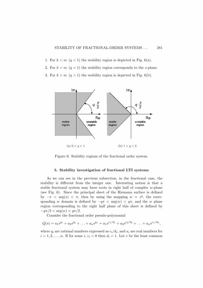
Definition 2. Mapping the poles from the sq-plane into the w-plane,where q ∈ Q such as q = k

m for k,m ∈ N and |arg(w)| = |φ|, can be doneby the following rule: If we assume k = 1, then the mapping from s-planeto w-plane is independent of k. Unstable region from s-plane transforms tosector |φ| < π

2m and stable region transforms to sector π2m < |φ| < π

m . Theregion where |φ| > π

m is not physical. Therefore, the system will be stableif all roots in the w-plane lie in the region |φ| > π

2m . The stability regionsdepicted in Fig. 6 correspond to the following propositions:


1. For k < m (q < 1) the stability region is depicted in Fig. 6(a).

2. For k = m (q = 1) the stability region corresponds to the s-plane.

3. For k > m (q > 1) the stability region is depicted in Fig. 6(b).

(a) 0 < q < 1 (b) 1 < q < 2

Figure 6: Stability regions of the fractional order system.

5. Stability investigation of fractional LTI systems

As we can see in the previous subsection, in the fractional case, thestability is different from the integer one. Interesting notion is that astable fractional system may have roots in right half of complex w-plane(see Fig. 6). Since the principal sheet of the Riemann surface is definedby −π < arg(s) < π, then by using the mapping w = sq, the corre-sponding w domain is defined by −qπ < arg(w) < qπ, and the w planeregion corresponding to the right half plane of this sheet is defined by−qπ/2 < arg(w) < qπ/2.

Consider the fractional order pseudo-polynomial

Q(s) = a1sq1 + a2s

q2 + . . . + ansqn = a1sc1/d1 + a2s

c2/d2 + . . . + anscn/dn ,

where qi are rational numbers expressed as ci/di, and ai are real numbers fori = 1, 2, . . . , n. If for some i, ci = 0 then di = 1. Let v be the least common

282 I. Petras

multiple (LCM) of d1, d2, . . . , dn, denoted as v = LCMd1, d2, . . . , dn, then( [24]):

Q(s) = a1sv1v + a2s

v2v + . . . + ans

vnv = a1(s

1v )v1 + a2(s

1v )v2 + . . . + an(s

1v )vn .(28)

The fractional degree (FDEG) of the polynomial Q(s) is defined as ( [24]):

FDEGQ(s) = maxv1, v2, . . . , vn.

The domain of definition for (28) is the Riemann surface with v Riemannsheets where origin is a branch point of order v − 1 and the branch cut isassumed at R−. The number of roots for the fractional algebraic equation(28) is given by the following proposition, [8]: Let Q(s) be a fractional orderpolynomial with FDEGQ(s) = n. Then the equation Q(s)=0 has exactlyn roots on the Riemann surface.

Definition 3. The fractional order polynomial

Q(s) = a1snv + a2s

n−1v + . . . + ans

1v + an+1

is minimal if FDEGQ(s) = n. We will assume that all fractional orderpolynomials are minimal. This ensures that there is no redundancy in thenumber of the Riemann sheets [24].

On the other hand, it has been shown, by several authors and by usingseveral methods, that for the case of FOLTI system of commensurate order,a geometrical method of complex analysis based on the argument principleof the roots of the characteristic equation (a polynomial in this particularcase) can be used for the stability check in the BIBO sense (see e.g. [35,44]).The stability condition can then be stated as follows [34,35,56]:

Theorem 1. A commensurate order system described by a rationaltransfer function (6) is stable if only if

|arg (λi)| > απ

2, for all i

with λi the i-th root of P (sα).

P r o o f. For proof see [34].For the FOLTI system with commensurate order where the system poles

are in general complex conjugate, the stability condition can also be ex-pressed as follows [34,35]:


Theorem 2. A commensurate order system described by a rationaltransfer function

G(w) =Q(w)P (w)

,

where w = sq, q ∈ R+, (0 < q < 2), is stable if only if

|arg (wi)| > qπ

2,

with ∀wi ∈ C the i-th root of P (w) = 0.

P r o o f. For proof see [35].When w = 0 is a single root (singularity at the origin) of P , the system

cannot be stable. For q = 1, this is the classical theorem of pole locationin the complex plane: have no pole in the closed right half plane of thefirst Riemann sheet. The stability region suggested by this theorem tendsto the whole s-plane when q tends to 0, corresponds to the Routh-Hurwitzstability when q = 1, and tends to the negative real axis when q tends to 2.

Theorem 3. It has been shown that commensurate system (14) is sta-ble if the following condition is satisfied (also if the triplet A, B, C isminimal) [4, 35,59–61]:

|arg(eig(A))| > qπ

2, (29)

where 0 < q < 2 and eig(A) represents the eigenvalues of matrix A.

P r o o f. For proof see [35].

Definition 4. We assume, that some incommensurate order systemsdescribed by the FODE (8) or (14), can be decomposed to the followingmodal form of the fractional transfer function (the so called Laguerre func-tions, [5]):

F (s) =N∑

i=1

nk∑

k=1

Ai,k

(sqi + λi)k(30)

for some complex numbers Ai,k, λi, and positive integer nk.A system (30) is BIBO stable if and only if qi and the argument of λi

denoted by arg(λi) in (30) satisfy the inequalities

0 < qi < 2 and |arg (λi)| < π

(1− qi

2

)for all i. (31)

Henceforth, we will restrict the parameters qi to the interval qi ∈ (0, 2). Forthe case qi = 1 for all i we obtain a classical stability condition for integer

284 I. Petras

order system (no pole is in right half plane). The inequalities (31) wereobtained by applying the stability results given in [1, 35].

Theorem 4. Consider the following autonomous system for internalstability definition:

0Dqt x(t) = Ax(t), x(0) = x0, (32)

with q = [q1, q2, . . . , qn]T and its n-dimensional representation:

0Dq1t x1(t) = a11x1(t) + a12x2(t) + . . . + a1nxn(t)

0Dq2t x2(t) = a21x1(t) + a22x2(t) + . . . + a2nxn(t)

. . .

0Dqnt xn(t) = an1x1(t) + an2x2(t) + . . . + annxn(t) (33)

where all qi’s are rational numbers between 0 and 2. Assume m be theLCM of the denominators ui’s of qi’s , where qi = vi/ui, vi, ui ∈ Z+ fori = 1, 2, . . . , n and we set γ = 1/m. Define [16]:

det

λmq1 − a11 −a12 . . . −a1a

−a21 λmq2 − a22 . . . −a2n

. . .−an1 −an2 . . . λmqn − ann

= 0. (34)

The characteristic equation (34) can be transformed to integer order poly-nomial equation if all qi’s are rational number. Then the zero solution ofsystem (33) is globally asymptotically stable if all roots λi’s of the charac-teristic (polynomial) equation (34) satisfy

|arg(λi)| > γπ

2for all i.

Denoting λ by sγ in equation (34), we get the characteristic equation inthe form det(sγI −A) = 0.

P r o o f. This assumption was proved in [16].

Corollary 1. Suppose q1 = q2 = . . . , qn ≡ q, q ∈ (0, 2), all eigenvaluesλ of matrix A in (14) satisfy |arg(λ)| > qπ/2, the characteristic equationbecomes det(sqI − A) = 0 and all characteristic roots of the system (14)have negative real parts [16]. This result is Theorem 1 of paper [34].


Remark 1. Generally, when we assume s = |r|eiφ, where |r| is modulusand φ is argument of complex number in s-plane, respectively, transforma-tion w = s

1m to complex w-plane can be viewed as s = |r| 1

m eiφm and thus

|arg(s)| = m|arg(w)| and |s| = |w|m. The proof of this statement is obvious.

The stability analysis criteria for a general FOLTI system canbe summarized as follows:

The characteristic equation of a general LTI fractional order system ofthe form:

ansαn + . . . + a1sα1 + a0s

α0 ≡n∑

i=0

aisαi = 0 (35)

may be rewritten asn∑

i=0

aisuivi = 0

and transformed into the w-planen∑

i=0

aiwi = 0, (36)

with w = skm , where m is the LCM of vi. The procedure of stability analysis

is (see e.g. [51]):

1. For given ai calculate the roots of equation (36) and find the absolutephase of all roots |φw|.

2. Roots in the primary sheet of the w-plane which have correspondingroots in the s-plane can be obtained by finding all roots which lie inthe region |φw| < π

m then applying the inverse transformation s = wm

(see Remark 1.). The region where |φw| > πm is not physical. For

testing the roots in desired region the matrix approach (19) can beused.

3. The condition for stability is π2m < |φw| < π

m . Condition for oscillationis |φw| = π

2m otherwise the system is unstable (see Fig. 5(b)). If thereis not root in the physical s-plane, the system will always be stable.

Example 4. Let us consider the linear fractional order LTI systemdescribed by the transfer function [17,48]:

G(s) =Y (s)U(s)

=1

0.8s2.2 + 0.5s0.9 + 1, (37)

286 I. Petras

and let the corresponding FODE have the following form:

0.8 0D2.2t y(t) + 0.5 0D

0.9t y(t) + y(t) = u(t) (38)

with zero initial conditions.The system (38) can be rewritten to its state space representation (x1(t) ≡

y(t)):[

0D910 x1(t)

0D1310 x2(t)

]=

[0 1

−1/0.8 −0.5/0.8

] [x1(t)x2(t)

]+

[0

1/0.8

]u(t)

y(t) =[

1 0] [

x1(t)x2(t)

](39)

The eigenvalues of the matrix A are λ1,2 = −0.3125 ± 1.0735j and then|arg(λ1,2)| = 1.8541. Because of various derivative orders in (39), Theorem3 cannot be used directly.

0 5 10 15 20 25 30 35 40 45 50−8

−6

−4

−2

0

2

4

6

8

10x 10

−3

Time (sec)

y(t)

Figure 7: Analytical solution of the FODE (38), where u(t) = 0 for 50 s andzeros initial conditions.

The analytical solution of the FODE (38) for u(t) = 0 obtained fromgeneral solution (10) has the form:

y(t) =1

0.8

∞∑

k=0

(−1)k

k!

(1

0.8

)k

Ek(t,−0.50.8

; 2.2− 0.9, 2.2 + 0.9k). (40)


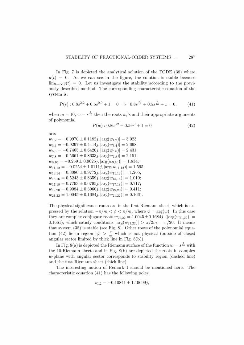
In Fig. 7 is depicted the analytical solution of the FODE (38) whereu(t) = 0. As we can see in the figure, the solution is stable becauselimt→∞y(t) = 0. Let us investigate the stability according to the previ-ously described method. The corresponding characteristic equation of thesystem is:

P (s) : 0.8s2.2 + 0.5s0.9 + 1 = 0 ⇒ 0.8s2210 + 0.5s

910 + 1 = 0, (41)

when m = 10, w = s110 then the roots wi’s and their appropriate arguments

of polynomialP (w) : 0.8w22 + 0.5w9 + 1 = 0 (42)

are:w1,2 = −0.9970± 0.1182j, |arg(w1,2)| = 3.023;w3,4 = −0.9297± 0.4414j, |arg(w3,4)| = 2.698;w5,6 = −0.7465± 0.6420j, |arg(w5,6)| = 2.431;w7,8 = −0.5661± 0.8633j, |arg(w7,8)| = 2.151;w9,10 = −0.259± 0.9625j, |arg(w9,10)| = 1.834;w11,12 = −0.0254± 1.0111j, |arg(w11,12)| = 1.595;w13,14 = 0.3080± 0.9772j, |arg(w11,12)| = 1.265;w15,16 = 0.5243± 0.8359j, |arg(w15,16)| = 1.010;w17,18 = 0.7793± 0.6795j, |arg(w17,18)| = 0.717;w19,20 = 0.9084± 0.3960j, |arg(w19,20)| = 0.411;w21,22 = 1.0045± 0.1684j, |arg(w21,22)| = 0.1661.

The physical significance roots are in the first Riemann sheet, which is ex-pressed by the relation −π/m < φ < π/m, where φ = arg(w). In this casethey are complex conjugate roots w21,22 = 1.0045±0.1684j (|arg(w21,22)| =0.1661), which satisfy conditions |arg(w21,22)| > π/2m = π/20. It meansthat system (38) is stable (see Fig. 8). Other roots of the polynomial equa-tion (42) lie in region |φ| > π

m which is not physical (outside of closedangular sector limited by thick line in Fig. 8(b)).

In Fig. 8(a) is depicted the Riemann surface of the function w = s110 with

the 10-Riemann sheets and in Fig. 8(b) are depicted the roots in complexw-plane with angular sector corresponds to stability region (dashed line)and the first Riemann sheet (thick line).

The interesting notion of Remark 1 should be mentioned here. Thecharacteristic equation (41) has the following poles:

s1,2 = −0.10841± 1.19699j,

288 I. Petras

−1

−0.5

0

0.5

1

−1

−0.5

0

0.5

1−1

−0.5

0

0.5

1

(a) 10-sheets Riemann surface

−1 −0.5 0 0.5 1 1.5−1.5

−1

−0.5

0

0.5

1

1.5

Re(w)Im

(w) π/20

−π/20

(b) Poles in complex w-plane

Figure 8: Riemann surface of function w = s110 and roots of equation (42).

in the first Riemann sheet in s-plane, which can be obtained e.g. via theMATLAB routine, as for instance:

>>s=solve(’0.8*s^2.2+0.5*s^0.9+1=0’,’s’)

When we compare |arg(w21,22)| = 0.1661 and |arg(s1,2)| = 1.661, we can seethat |arg(s1,2)| = m|arg(w21,22)|, where m = 10 in transformation w = s

1m .

The first Riemann sheet is transformed from the s-plane to the w-plane asfollows: −π/10 < arg(w) < π/10 and in order to −π < 10 arg(w) < π.Therefore from this consideration we then obtain |arg(s)| = 10 |arg(w)|.

Example 5. Let us examine an interesting example of application, theso called Bessel function of the first kind, which transfer function is ( [35]):

H(s) =1√

s2 + 1∀s, <(s) > 0. (43)

We have two branch points s1 = i, and s2 = −i and two cuts. One along thehalf line (−∞+i, i) and another one along the half line (−∞−i,−i). In thisdoubly cut complex plane, we have the identity

√s2 + 1 =

√s− i

√s + i.

The well known asymptotic expansion of equation (43) is:

h(t) ≈√

2πt

cos(t− π

4) =

√2π

t−12 E2,1

(−(t− π

4)2

).


According to the branch points and the above asymptotic expansion, we canstate that the system described by the Bessel function (43) is on boundaryof stability and has oscillation behaviour.

Example 6. Consider the closed loop system with controlled system(electrical heater)

G(s) =1

39.96s1.25 + 0.598(44)

and integer order controller

C(s) = 64.47 + 12.46s. (45)

The resulting closed loop transfer function Gc(s) becomes ( [47]):

Gc(s) =Y (s)W (s)

=12.46s + 64.47

39.69s1.25 + 12.46s + 65.068. (46)

The analytical solution (impulse response) of the fractional order controlsystem (46) is:

y(t) =12.4639.69

∞∑

k=0

(−1)k

k!

(12.4639.69

)k

× Ek(t,−65.06839.69

; 1.25, 0.25− k) (47)

+64.4739.69

∞∑

k=0

(−1)k

k!

(65.06839.69

)k

× Ek(t,−12.4639.69

; 1.25− 1, 1.25 + k)

with zero initial conditions.The characteristic equation of this system is

39.69s1.25 +12.46s+65.068 = 0 ⇒ 39.69s54 +12.46s

44 +65.068 = 0. (48)

Using the notation w = s1m , where LCM is m = 4, we obtain a polynomial

of complex variable w in the form

39.69w5 + 12.46w4 + 65.068 = 0. (49)

Solving the polynomial (49) we get the following roots and their arguments:

w1 = −1.17474, |arg(w1)| = π,

w2,3 = −0.40540± 1.0426j, |arg(w2,3)| = 1.9416,

w4,5 = 0.83580± 0.64536j, |arg(w4,5)| = 0.6575.

This first Riemann sheet is defined as a sector in w-plane within interval−π/4 < arg(w) < π/4. The complex conjugate roots w4,5 lie in this inter-val and satisfy the stability condition given as |arg(w)| > π

8 , therefore thesystem is stable. The region where |arg(w)| > π

4 is not physical.

290 I. Petras

6. Stability investigation of fractional nonlinear systems

As it has been mentioned in [34], the exponential stability cannot beused to characterize the asymptotic stability of fractional order systems. Anew definition was introduced in [41].

Definition 5. The trajectory x(t) = 0 of the system (16) is t−q

asymptotically stable if there is a positive real q such that:

∀||x(t)|| with t ≤ t0, ∃N(x(t)), such that ∀t ≥ t0, ||x(t)|| ≤ Nt−q.

The fact that the components of x(t) slowly decay towards 0 following t−q

leads to fractional systems sometimes being called long memory systems.The power law stability t−q is a special case of the Mittag-Leffler stability[31].

According to the stability theorem from [63], the equilibrium pointsare asymptotically stable for q1 = q2 = . . . = qn ≡ q if all the eigen-values λi, (i = 1, 2, . . . , n) of the Jacobian matrix J = ∂f/∂x, where f =[f1, f2, . . . , fn]T , evaluated at the equilibrium, satisfy the condition ([59,60]):

|arg(eig(J))| = |arg(λi)| > qπ

2, i = 1, 2, . . . , n. (50)

Fig. 6 shows stable and unstable regions of the complex plane for such case.Now, consider the incommensurate fractional order system q1 6= q2 6=

. . . 6= qn and suppose that m is the LCM of the denominators ui’s of qi’s,where qi = vi/ui, vi, ui ∈ Z+ for i = 1, 2, . . . , n and we set γ = 1/m. System(17) is asymptotically stable if:

|arg(λ)| > γπ

2

for all roots λ of the following equation

det(diag([λmq1 λmq2 . . . λmqn ])− J) = 0. (51)

A necessary stability condition for fractional order systems (17) to re-main chaotic is keeping at least one eigenvalue λ in the unstable region [60].The number of saddle points and eigenvalues for one-scroll, double-scrolland multi-scroll attractors was exactly described in the work [61]. Assumethat a 3D chaotic system has only three equilibria. Therefore, if the systemhas double-scroll attractor, it has two saddle points surrounded by scrollsand one additional saddle point. Suppose that the unstable eigenvalues of


scroll saddle points are: λ1,2 = α1,2 ± jβ1,2. The necessary condition toexhibit double-scroll attractor of system (17) is the eigenvalues λ1,2 remain-ing in the unstable region [61]. The condition for commensurate derivativesorder is

q >2π

atan( |βi|

αi

), i = 1, 2. (52)

This condition can be used to determine the minimum order for which anonlinear system can generate chaos [60]. In other words, when the instabil-ity measure π/2m−min(|arg(λ)|) is negative, the system can not be chaotic.

Example 7. Let us investigate the Chen’s system with a double scrollattractor. The fractional order form of such system can be described as [63]

0D0.8t x1(t) = 35[x2(t)− x1(t)],

0D1.0t x2(t) = −7x1(t)− x1(t)x3(t) + 28x2(t),

0D0.9t x3(t) = x1(t)x2(t)− 3x3(t). (53)

The system has three equilibria at (0, 0, 0), (7.94, 7.94, 21), and (−7.94,−7.94, 21). The Jacobian matrix of the system evaluated at (x∗1, x∗2, x∗3)is:

J =

−35 35 0−7− x∗3 28 −x∗1

x∗2 x∗1 −3

. (54)

The two last equilibrium points are saddle points and surrounded by achaotic double scroll attractor. For these two points, equation (51) becomesas follows:

λ27 + 35λ19 + 3λ18 − 28λ17 + 105λ10 − 21λ8 + 4410 = 0. (55)

The characteristic equation (55) has unstable roots λ1,2 = 1.2928±0.2032j,|arg(λ1,2)| = 0.1560 and therefore system (53) satisfies the necessary con-dition for exhibiting a double scroll attractor. The instability measure is0.0012.

Numerical simulation result of the system (53) for initial conditions(−9,−5, 14), obtained via approximation technique described in [17], forsimulation time 30 s and time step h = 0.0005, is depicted in Fig. 9.

292 I. Petras

−20

−10

0

10

20−20

−100

1020

30

0

5

10

15

20

25

30

35

40

x2(t)

x1(t)

x 3(t)

Figure 9: Double scroll attractor of Chen’s system (53) in state space.

7. Conclusions

In this paper we have presented the definitions for internal and externalstability condition of certain class of the linear and nonlinear fractional ordersystem of finite dimension given in state space, FODE or transfer functionrepresentation (polynomial). It is important to note that the stability andasymptotic behavior of fractional order system is not of exponential type [11]but it is in the form of power law t−α (α ∈ R), the so called long memorybehavior [34].

The results presented in this survey are also applicable in the robuststability investigation [22, 45–47], stability of delayed system [16, 21] andstability of discrete fractional order system [19, 35]. Investigation of thefractional incommensurate order systems in state space, where space is de-formed by various order of derivatives in various directions is still openproblem.

Acknowledgements

This work was partially supported by the Slovak Grant Agency for Sci-ence under Grants VEGA: 1/4058/07, 1/0365/08, 1/0404/08, and ProjectAPVV-0040-07.


References

[1] H. Akcay and R. Malti, On the completeness problem for fractionalrationals with incommensurable differentiation orders. In: Proc. of the17th World Congress IFAC, Soul, Korea, July 6-11 (2008), 15367–15371.

[2] E. Ahmed, A. M. A. El-Sayed and Hala A. A. El-Saka, On some Routh-Hurwitz conditions for fractional order differential equations and theirapplications in Lorenz, Rossler, Chua and Chen systems. Physics Let-ters A 358 (2006), 1–4.

[3] B. D. O.Anderson, N. I. Bose and E. I.Jury, A simple test for zeros ofa complex polynomial in a sector. IEEE Transactions on AutomaticControl, Tech. Notes and Corresp. AC-19 (1974), 437-438.

[4] M. Aoun, R. Malti, F. Levron and A. Oustaloup, Numerical simu-lations of fractional systems: An overview of existing methods andimprovements. Nonlinear Dynamics 38 (2004), 117-131.

[5] M. Aoun, R. Malti, F. Levronc and A. Oustaloup, Synthesis of frac-tional Laguerre basis for system approximation. Automatica 43 (2007),1640–1648.

[6] P. Arena, R. Caponetto, L. Fortuna and D. Porto, Nonlinear Nonin-teger Order Circuits and Systems - An Introduction. World Scientific,Singapore (2000).

[7] M. Axtell and E. M. Bise, Fractional calculus applications in controlsystems. In: Proc. of the IEEE 1990 Nat. Aerospace and ElectronicsConf., New York (1990), 563–566.

[8] F. M.-Bayat, M. Afshar and M. K.-Ghartemani, Extension ofthe root-locus method to a certain class of fractional-order sys-tems. ISA Transactions 48, Issue 1 (Jan. 2009), 48-53 (Elsevier,doi:10.1016/j.isatra.2008.08.001).

[9] F. M.-Bayat and M. Afshar, Extending the Root-Locus Methodto Fractional-Order Systems. Journal of Applied Mathematics,2008 (2008), Article ID 528934, 13p. (Hindawi Publ. Corp.,doi:10.1155/2008/528934).

[10] F. M.-Bayat and M. K.-Ghartemani, On the essential instabilitiescaused by multi-valued transfer functions. Math. Problems in Engi-neering 2008 (2008), Article ID 419046, 13p. (Hindawi Publ. Corp.).

[11] R. Bellman, Stability theory of differential equations. McGraw-HillBook Company, New York (1953).

294 I. Petras

[12] H. W. Bode, Network Analysis and Feedback Amplifier Design. TungHwa Company (1949).

[13] C. Bonnet and J. R. Partington, Coprime factorizations and stability offractional differential systems. Systems and Control Letters 41 (2000),167-174.

[14] M. Caputo, Linear models of dissipation whose Q is almost frequencyindependent. Geophys. J. R. Astr. Soc. 13 (1967), 529-539 (Reprintedrecently in: Fract. Calc. Appl. Anal. 11, No 1 (2008), 3–14).

[15] G. E. Carlson and C. A. Halijak, Approximation of fractional capac-itors (1/s)1/n by a regular Newton process. IEEE Trans. on CircuitTheory 11 (1964), 210–213.

[16] W. Deng, Ch. Li and J. Lu, Stability analysis of linear fractional dif-ferential system with multiple time delays. Nonlinear Dynamics 48(2007), 409-416.

[17] L. Dorcak, Numerical Models for Simulation the Fractional-Order Con-trol Systems, UEF-04-94, The Academy of Sciences, Inst. of Experi-mental Physic, Kosice, Slovakia (1994).

[18] R. C. Dorf and R. H. Bishop, Modern Control Systems. Addison-Wesley, New York (1990).

[19] A. Dzieliski and D. Sierociuk, Stability of discrete fractional orderstate-space systems. Journal of Vibration and Control 14 (2008),1543–1556.

[20] A. Charef, Modeling and analog realization of the fundamental linearfractional order differential equation. Nonlinear Dynamics 46 (2006),195-210.

[21] Y. Q. Chen and K. L. Moore, Analytical stability bound for a classof delayed fractional-order dynamic systems. Nonlinear Dynamics 29(2002), 191-200.

[22] Y. Q. Chen H. -S. Ahna and D. Xue, Robust controllability of intervalfractional order linear time invariant systems. Signal Processing 86(2006), 2794-2802.

[23] S. A. Abd El-Salam and A. M. A. El-Sayed, On the stability ofsome fractional-order non-autonomous systems. Electr. J. of Quali-tative Theory of Diff. Equations 6 (2007), 1–14.

[24] M. K. Ghartemani and F. M. Bayat, Necessary and sufficient con-ditions for perfect command following and disturbance rejection infractional order systems. In: Proc. of the 17th World Congress IFAC,Soul, Korea, July 6-11 (2008), 364–369.


[25] R. Gorenflo, Yu. Luchko and S. Rogosin. Mittag-Leffler type functions:Notes on growth properties and distribution of zeros, Preprint No. A-97-04, Freie Univ. Berlin, Germany (2004).

[26] B.Gross and E.P. Braga, Singularities of Linear System Functions.Elsevier Publishing, New York (1961).

[27] S. E. Hamamci, Stabilization using fractional-order PI and PID con-trollers. Nonlinear Dynamics 51 (2008), 329-343.

[28] Ch. Hwang and Y. -Ch. Cheng, A numerical algorithm for stabilitytesting of fractional delay systems. Automatica 42 (2006), 825-831.

[29] I. S. Jesus and J. A. T. Machado, Fractional control of heat diffu-sion systems. Nonlinear Dynamics 54, No 3 (Nov. 2008), 263–282(doi:10.1007/s11071-007-9322-2).

[30] W. R. LePage, Complex Variables and the Laplace Transform for En-gineers. McGraw-Hill (1961).

[31] Y. Li, Y.Q.Chen, I. Podlubny and Y. Cao, Mittag-Leffler stability offractional order nonlinear dynamic system. In: Proc. of the 3rd IFACWorkshop on Fractional Differentiation and its Applications, Ankara,Turkey, 05-07 November (2008).

[32] B. J. Lurie, Three-Parameter Tunable Tilt-Integral-Derivative (TID)Controller, United States Patent, 5 371 670, USA (1994).

[33] S. Manabe, The non-integer integral and its application to controlsystems. ETJ of Japan 6 (1961), 83–87.

[34] D. Matignon, Stability result on fractional differential equations withapplications to control processing. In: IMACS-SMC Proceedings, Lille- France (July 1996), 963-968.

[35] D. Matignon, Stability properties for generalized fractional differentialsystems. In: Proc. of Fractional Differential Systems: Models, Methodsand App. 5 (1998), 145–158.

[36] D. Matignon and B. D’Andrea-Novel, Some results on controllabilityand observability of finite-dimensional fractional differential systems.In: Computational Engineering in Systems Applications, Vol. 2, Lille- France (1996), 952–956.

[37] C. A. Monje, B. M. Vinagre, V. Feliu and Y. Q. Chen, Tuning andauto-tuning of fractional order controllers for industry applications.IFAC J. of Control Engineering Practice 16 (2008), 798–812.

[38] M. Nakagava and K. Sorimachi, Basic characteristics of a fractancedevice. IEICE Trans. Fundamentals E75 - A (1992), 1814–1818.

296 I. Petras

[39] K. B. Oldham and J. Spanier, The Fractional Calculus. AcademicPress, New York (1974).

[40] A. Oustaloup, La Derivation Non Entiere: Theorie, Synthese et Ap-plications. Hermes, Paris (1995).

[41] A. Oustaloup, J. Sabatier, P. Lanusse, R. Malti, P. Melchior,X. Moreau and M. Moze, An overview of the CRONE approach insystem analysis, modeling and identification, observation and control.In: Proc. of the 17th World Congress IFAC, Soul, Korea, July 6-11(2008), 14254–14265.

[42] N. Ozturk and A. Uraz, An analysis stability test for a certain classof distributed parameter systems with delay. IEEE Trans. on Circuitand Systems CAS-32 (1985), 393–396.

[43] F. J. V. -Parada, J. A. O. -Tapia and J. A. -Ramirez, Effective mediumequations for fractional Ficks law in porous media. Physica A 373(2007), 339–353.

[44] I. Petras and L. Dorcak, The frequency method for stability investiga-tion of fractional control systems, J. of SACTA, 2 (1999), 75–85.

[45] I. Petras, Y. Q. Chen and B. M. Vinagre, A robust stability test pro-cedure for a class of uncertain LTI fractional order systems. In: Proc.of the Intern. Carpathian Control Conf., Malenovice, Czech republic,May 27-30 (2002), 247–252.

[46] I. Petras, Y. Q. Chen and B. M. Vinagre, Robust stability test for in-terval fractional order linear systems. Volume 208-210, Chapter 6.5: V.D. Blondel and A. Megretski (Eds.), Unsolved Problems in the Math-ematics of Systems and Control, Princeton University Press (2004).

[47] I. Petras, Y. Q. Chen, B. M. Vinagre and I. Podlubny, Stability of lin-ear time invariant systems with interval fractional orders and intervalcoefficients. In: Proc. of the Intern. Conf. on Computation Cybernet-ics, Vienna, Austria, 8/30-9/1 (2004), 1-4.

[48] I. Podlubny, Fractional Differential Equations. Academic Press, SanDiego (1999).

[49] I. Podlubny, Geometric and physical interpretation of fractional in-tegration and fractional differentiation. Fract. Calc. Appl. Anal. 5(2002), 367-386.

[50] I. Podlubny, Fractional-order systems and PIλDµ-controllers. IEEETrans. on Automatic Control 44 (1999), 208-213.


[51] A. G. Radwan, A. M. Soliman, A. S. Elwakil and A. Sedeek,On the stability of linear systems with fractional-order elements.Chaos, Solitons & Fractals 40, Issue 5 (June 2009), 2317-2328(doi:10.1016/j.chaos.2007.10.033).

[52] H.F. Raynaud and A. Zergaınoh, State-space representation for frac-tional order controllers. Automatica 36 (2000), 1017–1021.

[53] M. F. Silva, J. A. T. Machado and A. M. Lopes, Fractional ordercontrol of a hexapod robot. Nonlinear Dynamics 38 (2004), 417-433.

[54] B. M. Vinagre, Y. Q. Chen and I. Petras, Two direct Tustin discretiza-tion methods for fractional-order differentiator/integrator. J. FranklinInstitute 340 (2003), 349–362.

[55] B. M. Vinagre, I. Petras, P. Merchan and L. Dorcak, Two digital re-alizations of fractional controllers: Application to temperature controlof a solid. In: Proc. of the ECC’01, Porto, Portugal, September 4 - 7(2001), 1764–1767.

[56] B. M. Vinagre and V. Feliu, Optimal fractional controllers for rationalorder systems: A special case of the Wiener-Hopf spectral factorizationmethod. IEEE Trans. on Automatic Control 52 (2007), 2385-2389.

[57] B. M. Vinagre, C. A. Monje, A. J. Calderon and J. I. Suarez, FractionalPID controllers for industry application. A brief introduction. J. ofVibration and Control 13 (2007), 1419–1429.

[58] J. A. O-Tapia, F. J. V. -Parada and J. A. -Ramirez, A fractional-orderDarcys law. Physica A 374 (2007), 1-14.

[59] M. S. Tavazoei and M. Haeri, Unreliability of frequency-domain ap-proximation in recognising chaos in fractional-order systems. IET Sig-nal Proc. 1 (2007), 171–181.

[60] M. S. Tavazoei and M. Haeri, A necessary condition for double scrollattractor existence in fractional-order systems. Physics Letters A 367(2007), 102–113.

[61] M. S. Tavazoei and M. Haeri, Limitations of frequency domain ap-proximation for detecting chaos in fractional order systems. NonlinearAnalysis 69 (2008), 1299–1320.

[62] M. S. Tavazoei and M. Haeri, A note on the stability of fractional ordersystems. Mathematics and Computers in Simulation 79, Issue 5 (Jan.2009), 1566–1576 (doi: 10.1016/j.matcom.2008.07.003).

[63] M. S. Tavazoei and M. Haeri, Chaotic attractors in incommensuratefractional order systems. Physica D 237 (2008), 2628–2637.

298 I. Petras

[64] P. J. Torvik and R. L. Bagley, On the appearance of the FractionalDerivative in the Behavior of real materials. Transactions of the ASME51 (1984), 294–298.

[65] Ch. -Ch. Tseng, Design of FIR and IIR fractional order Simpson digitalintegrators. Signal Processing 87 (2007), 1045-1057.

[66] J. C. Wang, Realizations of generalized Warburg impedance with RCladder networks and transmission lines. J. of Electrochem. Soc. 34(1987), 1915–1920.

[67] S. Westerlund and L. Ekstam, Capacitor theory. IEEE Trans. on Di-electrics and Electrical Insulation 1 (1994), 826–839.

[68] S. Westerlund, Dead Matter Has Memory!. Causal Consulting, Kalmar(2002).

[69] D. Xue and Y. Q. Chen, A comparative introduction of four fractionalorder controllers, In: Proc. of the 4th World Congress on IntelligentControl and Automation, Shanghai, China, June 10-14 (2002).

Technical University of Kosice Received: November 25, 2008BERG FacultyInstitute of Control and Informatization of Production ProcessesB. Nemcovej 3, 042 00 Kosice – SLOVAKIA

e-mail: [email protected]

stability of fractional-order systems … of fractional-order systems with rational orders: a survey...

Documents