stability and stabilization of networked systems · une grande influence a la fois sur la...
TRANSCRIPT

NNT : 2017SACLS186
THESE DE DOCTORATDE
L’UNIVERSITE PARIS-SACLAYPREPAREE A
L’UNIVERSITE PARIS-SUD
Laboratoire des Signaux et Systemès
Ecole Doctorale N° 580Sciences et Technologies de l’Information et de la Communication (STIC)
Spécialité : Automatique
Par
MAGHENEM Mohamed Adlene
Stability and Stabilization of Networked Systems
Thèse soutenue à Gif-sur-Yvette, le 05/07/17.
Composition du jury :
M. Hassan Khalil Professor (Université d’état de Michigan) rapporteurM. Wei Ren Professor (Université de California Riverside) rapporteurM. Jamal Daafouz Professor (Université de Lorraine) président du juryM. Dragan Nesic Professor (Université de Melbourne) examinateurM. Lorenzo Marconi Professor (Université de Bologna) examinateurM. Fréderic Mazenc Directeur de recherche INRIA examinateurMme. Elena Panteley Directeur de recherche CNRS co-directeur de thèseM. Antonio Loría Directeur de recherche CNRS directeur de thèse

2
To Antonio Lorıaand Elena Panteley
with thanks.
Acknowledgments
Firstly, I would like to express my sincere gratitude to my advisors Antonio LORIA
and Elena PANTELEY for their continuous support during my Ph.D, their precious
advice, help and motivation. Their guidance brought me into the necessary scientific
rigor to do research in automatic control and helped me to improve the presentation
of my results, especially in this thesis. I could not have imagined having a better
advisors.
Besides, I would like to thank the members of my thesis committee starting by
Prof. Hassan KHALIL for his valuable and very insightful comments he provided
on this thesis. To Prof. Wei REN, Prof. Jamal DAAFOUZ, Prof. Frederic MAZENC,
Prof. Lorenzo MARCONI and Prof. Dragan NESIC, for their insightful comments,
their encouragement and the interesting questions they posed which incented me to
enlarge my research from various perspectives.
My sincere and warm thanks goes to Prof. Kristin Y.PETTERSEN from NTNU
Trondheim for providing me a great opportunity to join her laboratory and the fruitful
collaboration with her former Ph.D students Dennis BELLETER and Claudio PALIOTTA.
My thanks also go to Prof. Emmanuel NUNO ORTEGA from CUCEI Guadalajara
for welcoming me in his research group and making my visit to Guadalajara a pleasant
stay. To his former Msc student, my friend, Abraham CASTILLO BAUTISTA.
I appreciate Prof. Hassan KHALIL from Michigan state university and Prof. Wei
REN from U.C Riverside for accepting me to visit their laboratories and giving of their
precious time to exchange with them and with their research teams.
I would like to thank Prof. Manfredi MAGGIORE, Prof. Anuradha ANNASWAMY
and Dr. francoise LAMNABHI-LAGARRIGUE for being members of my midterm
3

4
evaluation committee and for the valuable advice and encouragement. The same
thanks goes to Prof. Yacine CHITOUR, Antoine CHAILLET and Wiliam PASSIAS
LEPINE for the stimulating discussions and the encouragements.
I thank all my fellows labmates I had the chance to meet for the inspiring discus-
sions and the fun we have had in the last three years. To: Dennis, Claudio, Abraham,
Roberto, Maria Fernanda, Gustavo, Erasmo, Derubo, Xiucai, Mehmet Akif, for their
help and hospitality. A special thanks go to my friends: Rafa, Pablo, Missie, Celia,
Mattia, Lorenzo, Juan, Lucien, Jonathon, Djawad, Tahar, Karim, Mohamed, Anis and
Rahim for their company and support.
To my high-school physics’ teacher Ali CHIKAOUI for his inspiring advises and
continuous support.
Last but not the least, to my family: my parents and sister for the spiritual support,
the motivation and personal advice they provided me throughout my studies.

Contents
Apercu de la these 9
Introduction and Motivation 13
Notations 21
1 Strict Lyapunov functions for time-varying systems with persistency of exci-
tation 23
1.1 Case-study: a comparison positive system . . . . . . . . . . . . . . . . . . 25
1.2 Case-study: Cascaded systems . . . . . . . . . . . . . . . . . . . . . . . . 30
1.2.1 Chain of single integrators . . . . . . . . . . . . . . . . . . . . . . . 30
1.2.2 Multivariable cascaded linear time-varying systems . . . . . . . . 34
1.3 Case-study: spiraling systems . . . . . . . . . . . . . . . . . . . . . . . . . 38
1.3.1 Case-study: “adaptive control” systems . . . . . . . . . . . . . . . 40
1.3.2 Case-study: “skew-symmetric” systems . . . . . . . . . . . . . . . 44
1.4 Conclusion . . . . . . . . . . . . . . . . . . . . . . . . . . . . . . . . . . . . 49
2 Leader-follower formation control of nonholonomic vehicles 51
2.1 Problem formulation . . . . . . . . . . . . . . . . . . . . . . . . . . . . . . 54
2.1.1 Single follower case . . . . . . . . . . . . . . . . . . . . . . . . . . 55
2.1.2 Multiple followers case . . . . . . . . . . . . . . . . . . . . . . . . 56
2.2 Example of torque controller . . . . . . . . . . . . . . . . . . . . . . . . . . 57
2.3 Leader-follower tracking . . . . . . . . . . . . . . . . . . . . . . . . . . . . 60
2.4 Leader-follower formation tracking control . . . . . . . . . . . . . . . . . 65
2.4.1 Example . . . . . . . . . . . . . . . . . . . . . . . . . . . . . . . . . 70
2.5 Leader-follower robust stabilization control . . . . . . . . . . . . . . . . . 72
2.6 Leader-follower robust agreement control . . . . . . . . . . . . . . . . . . 79
2.6.1 Example . . . . . . . . . . . . . . . . . . . . . . . . . . . . . . . . . 82
2.7 Conclusion . . . . . . . . . . . . . . . . . . . . . . . . . . . . . . . . . . . . 85
5
6
3 Leader-follower simultaneous tracking-agreement control of nonholonomic
vehicles 87
3.1 A larger class of controllers . . . . . . . . . . . . . . . . . . . . . . . . . . 88
3.1.1 Proof of Proposition 3.1 . . . . . . . . . . . . . . . . . . . . . . . . 91
3.2 Control under relaxed conditions on the reference velocities . . . . . . . 103
3.2.1 Proof of Proposition 3.2 . . . . . . . . . . . . . . . . . . . . . . . . 105
3.3 A leader-follower formation case . . . . . . . . . . . . . . . . . . . . . . . 113
3.4 Simulations . . . . . . . . . . . . . . . . . . . . . . . . . . . . . . . . . . . 116
3.5 Conclusion . . . . . . . . . . . . . . . . . . . . . . . . . . . . . . . . . . . . 118
4 Consensus-based formation control of nonholonomic robots under delayed
interconnections 123
4.1 Network model description . . . . . . . . . . . . . . . . . . . . . . . . . . 124
4.1.1 Node dynamics . . . . . . . . . . . . . . . . . . . . . . . . . . . . . 124
4.1.2 Interconnection Topology . . . . . . . . . . . . . . . . . . . . . . . 126
4.2 Problem formulation . . . . . . . . . . . . . . . . . . . . . . . . . . . . . . 126
4.3 Control design and stability analysis . . . . . . . . . . . . . . . . . . . . . 128
4.3.1 Undelayed partial consensus problem . . . . . . . . . . . . . . . . 130
4.3.2 Delayed partial consensus problem . . . . . . . . . . . . . . . . . 133
4.3.3 Undelayed full consensus problem . . . . . . . . . . . . . . . . . . 138
4.3.4 Delayed full consensus problem . . . . . . . . . . . . . . . . . . . 142
4.4 Conclusion . . . . . . . . . . . . . . . . . . . . . . . . . . . . . . . . . . . . 150
Conclusions & Future Work 153
A Basic notions 155
A.1 Preliminaries . . . . . . . . . . . . . . . . . . . . . . . . . . . . . . . . . . . 155
A.2 Uniform Stability notions . . . . . . . . . . . . . . . . . . . . . . . . . . . 155
A.3 ISS and Lyapunov characterization . . . . . . . . . . . . . . . . . . . . . . 157
A.4 integral ISS and Lyapunov characterization . . . . . . . . . . . . . . . . . 158
A.5 Strong iISS . . . . . . . . . . . . . . . . . . . . . . . . . . . . . . . . . . . . 159
A.6 Nonlinear output injection . . . . . . . . . . . . . . . . . . . . . . . . . . . 159
A.7 PE, δ-PE and Uniform δ-PE . . . . . . . . . . . . . . . . . . . . . . . . . . 163
B Proof of auxiliary results 165
B.1 Proof of theorem 1.1 . . . . . . . . . . . . . . . . . . . . . . . . . . . . . . 165
B.2 Proof of theorem 1.4 . . . . . . . . . . . . . . . . . . . . . . . . . . . . . . 168
B.3 Proof of Proposition 1.2 . . . . . . . . . . . . . . . . . . . . . . . . . . . . . 170

Apercu de la these 7
B.4 Proof complement for Proposition 2.1 . . . . . . . . . . . . . . . . . . . . 173
B.5 Proof of Proposition 2.2 . . . . . . . . . . . . . . . . . . . . . . . . . . . . . 177
B.6 Proof of Lemma 2.1 . . . . . . . . . . . . . . . . . . . . . . . . . . . . . . . 179
B.7 Proof of Lemma 3.2 . . . . . . . . . . . . . . . . . . . . . . . . . . . . . . . 182
B.8 New Filtration Lemma . . . . . . . . . . . . . . . . . . . . . . . . . . . . . 182
B.9 Proof of theorem 4.1 . . . . . . . . . . . . . . . . . . . . . . . . . . . . . . 186
B.10 Proof of theorem 4.2 . . . . . . . . . . . . . . . . . . . . . . . . . . . . . . 195
B.11 Proof of theorem 4.3 . . . . . . . . . . . . . . . . . . . . . . . . . . . . . . 199
B.12 Proof of theorem 4.4 . . . . . . . . . . . . . . . . . . . . . . . . . . . . . . 202
Bibliography 207

8

Apercu de la these
Ce memoire presente le travail accompli au cours des trois dernieres annees sur la
coordination des systemes multi-agents et, en particulier, sur le controle en formation
des vehicules non-holonomes. En generale, resoudre un probleme de coordination
distribuee pour un systeme multi-agent consiste a synthetiser l’entree de commande
pour chaque agent afin de permettre a certaines grandeurs d’interet dans le groupe de
systemes de realiser une tache commune, par exemple, former une certaine posture
geometrique, suivre un leader commun, ou bien decrire un comportement commun
en regime permanent (synchronisation).
Selon la procedure de conception des lois de commandes, deux types d’approches
se distinguent, les approches centralisees et les approches distribuees. Dans le premier
cas, chaque systeme recoit une information globale qui consiste en le comportement
de reference qu’il est sense produire en regime permanent. Dans ce cas, le probleme de
coordination entre les differents systemes est reduit a la commande en poursuite de
chaque systeme separement vers son comportement de reference. Dans l’approche
distribuee, l’entree de commande de chaque agent est concue en utilisant unique-
ment des informations locales qui proviennent d’un certain groupe d’agents appele le
groupe de voisins. L’interaction entre les agents se caracterise, des lors, par un graphe
de communication.
Les solutions distribuees aux problemes de coordination des systemes multiagents
ont ete largement etudiees en automatique, nous citons par exemple:
[43], [93], [22], [79] and [106], la derniere reference est un etat de l’art sur le sujet.
Deux axes principaux de recherche sont identifies dans le contexte de la coordina-
tion distribuee des systemes multi-agents. Le premier apparaıt lorsqu’on considere
la commande distribuee en presence de contraintes sur le processus de communi-
cation entre les agents, ce qui inclut le cas ou le transfert d’informations est unidi-
rectionnel [102], [90], variable dans le temps, on parle dans ce cas de graph temps-
variant [104], [73], ou affecte par des retards de transmission ou des echantillonnages [1].
Le second cas survient lorsqu’on considere la dynamique individuelle des agents, par
exemple, le cas general des systemes lineaires [54], les systemes non-lineaires iden-
9

10
tiques [40], ou les systemes non-lineaires heterogenes [98], [120].
Le probleme general de la coordination distribuee du mouvement d’un groupe
d’agents mobiles a ete aussi largement etudie dans le domaine de l’ingenierie automa-
tique au cours des dernieres decennies. Un tel interet est du a l’importance d’une telle
coordination dans de nombreuses applications, nous citons par exemple le cas des
robots mobiles [29], des vehicules aeriens sans pilote [32], des vehicules sous-marins
autonomes [13], satellites [57], aeronefs et engins spatiaux [103], etc.
Parmi les problemes les plus importants en coordination distribuee, deux categories
de problemes se distinguent:
Probleme de consensus sans leader. Dans ce cas, l’objectif est de parvenir a un
arrangement entre les coordonnees des agents et de les faire converger asymptotique-
ment vers une posture commune. Les agents peuvent echanger uniquement des in-
formations avec un certain nombre de voisins. Le probleme de consensus sans leader
a ete etudie, par exemple, pour le cas des systemes lineaires de premier ordre et de
second ordre [73], [56], [109], et aussi pour le cas de certaines classes de systemes non-
lineaires [90, 92, 120]. Dans certaines applications, l’arrangement entre les etats des
systemes differe legerement du consensus classique, dans le sens ou, au lieu de faire
converger les etats vers une valeur commune, les agents devraient former une pos-
ture geometrique qui pourrait etre constante ou variable dans le temps. Ce type de
probleme est souvent appele probleme de formation a base de consensus. Il convient
de souligner qu’un changement de coordonnees est souvent adopte afin de permettre
la transformation du probleme de formation en un probleme de consensus [29].
Probleme de consensus avec leader. L’objectif, dans ce cas, est de parvenir a un
arrangement entre les agents tout en poursuivant une trajectoire commune generee
par un agent leader. Comme dans le cas precedent, seule l’information concernant les
postures des agents voisins (qui peuvent inclure le leader) est accessible pour chaque
agent. L’interaction entre les agents, incluant le leader, se caracterise par un graphe
d’interconnexion augmente. Le plus souvent, le comportement du systeme leader a
une grande influence a la fois sur la conception des lois de commande et aussi sur
l’analyse de la boucle fermee.
Dans ce document, les deux problemes decrits ci-dessus sont etudies dans le cas
ou les agents sont des robots mobiles non-holonomes. La commande du robot mobile
non-holonome a ete un domaine de recherche tres actif en automatique non-lineaire au
cours des deux dernieres decennies, voir par exemple [49] pour un etat de l’art sur la
commande de ce type de systemes; En regle generale, la commande d’un robot mobile
non-holonome consiste a resoudre l’un des trois problemes suivants:
Le probleme general de poursuite. Il consiste a definir un robot virtuel qui genere

Introduction and contributions 11
une trajectoire de reference que le robot commande est doit poursuivre. En general,
les vitesses du robot leader sont des fonctions variables dans le temps, ainsi le systeme
en boucle fermee est le plus souvent non-lineaire et temps-variant – voir les chapitres
2-3.
Le probleme de stabilisation. Il consiste a stabiliser les trajectoires du robot vers
une posture de consigne constant. Ce probleme est pertinent en raison de la con-
trainte non-holonome qui empeche la resolution du probleme en utilisant des lois de
retroaction lisses et autonomes [15]. Le probleme de stabilisation peut etre reformule
en un probleme de leader-suiveur en introduisant un leader dont les vitesses sont
egales a zero.
Le probleme de poursuite-stabilisation simultanes. Il consiste a concevoir un
controleur unifie qui resout le probleme de leader-suiveur pour le cas general des
vitesses du leader — voir Chapitre 2 pour une discussion plus detaillee.
L’extension naturelle du probleme de stabilisation d’un vehicules non-holonomes
au cas multi-agent est le probleme de consensus sans leader qui est etudie dans le
chapitre 4 sous l’hypothese d’un graphe bidirectionnel connecte et d’une communi-
cation affectee par un retard variant dans le temps et borne. Le probleme de leader-
suiveur pour un groupe de robots mobiles a egalement ete considere dans cette these.
Selon les vitesses du leader, Les chapitres 2 et 3 etudient les trois problemes suivants,
sous l’hypothese d’un graphe constant ayant une topologie particuliere qui est celle
de l’arbre generateur dirige.
1)- Probleme de poursuite leader-suiveur. Dans ce cas, on resout le probleme
de consensus leader-suiveur en supposant que les vitesses du leader decrivent une
function general variante dans le temps, de sorte que la norme de ses vitesses est un
signal a excitation permanente – voir Definition A.6.
2)- Probleme de rendez-vous robuste leader-suiveur. Dans ce cas, les vitesses du
leader convergent vers zero.
3)- Probleme de poursuite-rendez-vous simultanes. Dans ce cas, on propose un
controleur unifie qui resout le probleme de consensus leader-suiveur pour toutes les
configurations possibles des vitesses du leader.
Notre approche consiste a transformer chacun des problemes cites precedemment
en un probleme de stabilisation d’un ensemble invariant. Nos outils d’analyse re-
posent principalement sur la construction de fonctions de Lyapunov et de Lyapunov-
Krasovskii strictes pour des systemes non-lineaires variant dans le temps et/ou re-
tardes. Ces fonctions sont, par la suite, utilisees pour etablir des resultats de stabilite
uniforme et de robustesse pour le cas des robots mobiles.
Le premier chapitre de ce manuscrit presente des resultats techniques sur la sta-
12
bilite des systemes lineaires temps-variant inspirees du livre [72]. Notamment, on
presente les methodes essentielles pour la construction de fonctions de Lyapunov
strictes. Ces methodes sont employees dans tous les chapitres qui suivent pour la con-
ception des lois de commande et pour analyse de stabilite de la boucle fermee pour le
cas des robots mobiles en formation distribuee.
Introduction and Contributions
We present in this memoir the work accomplished in the last three years on multi-
agent coordination and in particular, on formation control of non-holonomic vehicles.
Generally speaking, solving multi-agent coordination problem consists on designing
the control input for each agent in order to allow certain quantities of interest in the
group of systems to realize a common task, for example, reaching a certain geomet-
ric pattern, following a common leader agent or describing a common steady state
behavior.
Depending on the control design procedure, we distinguish the centralized and the
distributed approaches. In the first approach each system receives a global information
which consists of its reference behavior. In this case, the multi-agent coordination
problem is reduced to the stabilization of each system separately toward its reference
behavior. In the distributed approach the control input for each agent is designed
using only local knowledge that is received from some agents called neighbors. The
interaction between the agents is characterized by a communication graph.
Distributed solution to multi-agent coordination, consensus or synchronization
problems have been extensively studied in the control literature, we cite for example:
[43], [93], [22], [79] and [106], where the last reference is a survey on this topic.
Two principle research axes can be identified in the context of distributed multi-
agent coordination. The first one appears when considering distributed control in
the presence of communication constraints between the agents, which include the
case when the transfer of information is unidirectional [102], [90], unreliable links
with time-varying graph topology [104], [73], delayed or sampled transfer of infor-
mation [1] to name few. The second one arises when considering individual dynamics
of the agents, for example, general linear systems [54], nonlinear homogeneous sys-
tems [40], or heterogeneous nonlinear systems [98], [120].
The general problem of distributed coordinated motion of mobile agents has been
extensively studied in control engineering during the last decades. Such an interest
is caused by importance of such a coordination in many different engineering ap-
plications, we cite here mobile robots [29], unmanned air vehicles [32], autonomous
13
14
underwater vehicles [13], satellites [57], aircraft and spacecraft [103], etc.
Among existing approaches to the coordination task we mention here the following
two problems:
Leaderless consensus problem. In this case the objective is to reach an agreement
between the agents and in particular coordinates to make them converge asymptoti-
cally to a common value. In this case, agents can exchange information only with their
neighbors. The leaderless consensus problem of multiple dynamical systems has been
extensively studied, for example, linear systems, including first, second order and
general linear systems are considered in [56,73,109], and different classes of nonlinear
systems are considered in [90, 92, 120].
In some applications, an agreement between the systems is slightly different from
the classical consensus, in the sense that instead of common value, the agents should
follow some geometric pattern that can be constant or time varying. This type of prob-
lem is often referred to as leaderless consensus problem. It should be underlined here
that an appropriate change of coordinates allows to transform the formation task into
consensus one [29].
Leader-follower consensus problem. In this case the objective is to reach an agree-
ment between the agents defined by a common trajectory generated by a leader agent.
As in the previous case only the information of the neighboring agents (and may be
the leader), is accessible to the agents. The interaction between the agents, including
the leader, is characterized by an augmented graph of interconnections. Usually, the
behavior of the leader system has a great influence both on the control design and on
the closed-loop analysis.
In this document we study the two above described problems in the case where the
agents are modeled as a nonholonomic mobile robots. The control of nonholonomic
mobile robot has been an active research field in the control community during the last
two decades see for example [49] for a survey on the control of nonholonomic vehicles;
generally speaking, controlling a nonholonomic mobile robot consists of solving one
of the following three problems.
The general leader-follower problem. It consists in defining a virtual robot that
generates a reference trajectory to be followed by the controlled robot. In general, the
velocities of the virtual robot are time varying functions, as a result the closed-loop
system is usually nonlinear and time varying–see Chapters 2-3.
The stabilization problem. It consists in stabilization of the robot trajectories to a
constant set point. This problem is relevant because of the nonholonomic restriction
that enables the use of any smooth autonomous feedback law [15]. The stabilization
problem can be recast as a leader-follower problem by introducing a leader, whose

Introduction and contributions 15
velocities are equal to zero.
The simultaneous tracking-stabilization problem. It consists in the design of a
unified controller that solves the leader-follower problem both in the case where the
leader’s velocities are either general time varying functions or equal to zero — see
Chapter 2 for more detailed discussion.
The natural extension of the stabilization problem for nonholonomic vehicles to
the multi-agent case is the leaderless consensus problem which we study in Chapter 4
under assumptions of a general bidirectional graph and time varying communication
delays. The leader-follower problem for a multiple nonholonomic mobile robots has
also been considered in this thesis. Depending on the leader’s velocities, Chapters 2
and 3 study the three following problems, respectively, under a particular constant
communication graph topology that is a directed spanning tree.
1)- Leader-follower tracking problem. In this case, we solve the leader-follower
consensus problem under the assumption that the leader vehicle describes a general
time varying path, such that, the norm of its velocities is persistently exciting,–see
Definition A.6.
2)- Leader-follower robust agreement problem. In this case, we solve the leader-
follower consensus problem when the leader’s velocities converge to zero.
3)- Simultaneous tracking-agreement problem. In this case, we design a unified
controller that solves the leader-follower consensus problem for all possible configu-
rations of the leader’s velocities.
Our approach consists in transforming each one of the problems cited above into a
stabilization problem of an invariant set. Our analysis tools are based, mainly, on the
construction of strict Lyapunov functions and strict Lyapunov-Krasovskii functionals
for nonlinear time varying and/or delayed systems. These functions are then used to
establish stability and robustness results in the area of mobile robot control.
The first chapter of this manuscript presents our basic technical results of stability
for time varying linear systems. Notably, we present therein the essential methods
for the construction of the strict Lyapunov functions. These methods we employ in
all the subsequent chapters in the control design and the analysis of mobile robots.
The Lyapunov functions that we employ follow ideas proposed in [72]. However, the
constructions that we present for the specific case-studies of time-varying systems in
Chapter 1, and for mobile robots, in the subsequent chapters, are original. Moreover,
to the best of our knowledge, for the problems of formation control for autonomous
vehicles, we are the first to provide strict Lyapunov functions.
Our contributions are described in further detail below.
16
Contributions of the thesis
We briefly summarize the main results of this thesis, chapter by chapter, and cite re-
lated publications. References correspond to the list of publications presented in p.
18.
• Chapter 1: We present some results on stability of persistently excited linear
time-varying systems with particular structures. Such systems appear in di-
verse problems, which include the analysis of model-reference adaptive systems,
persistently-excited observers, consensus of systems interconnected through time-
varying links and systems with time-varying input gain. The originality of our
statements lies in the fact that we provide smooth strict Lyapunov functions
hence, our proofs are constructive and direct. Moreover, we establish uniform
global exponential stability with explicit stability and decay estimates.
This chapter formed the subject of the following publications on: [(iv),(iii)].
• Chapter 2: We present controllers for leader-follower formation tracking and ro-
bust agreement control problems for a group of autonomous non-holonomic ve-
hicles. We consider general models composed of a velocity kinematics and a
generic force-balance equations. We assume that, each robot has a unique leader
and only the swarm leader robot knows the reference trajectory, but each robot
may have one or several followers. That is, the graph topology is a spanning
tree. For the tracking case, we establish uniform global asymptotic stability of the
closed-loop system under the assumption that the virtual vehicle velocities are
persistently exciting. The analysis relies on the construction of a strict Lyapunov
function for the position tracking error dynamics and a recursive argument for
cascaded systems. For the robust agreement case, we control the group of robots
that follow trajectories with a vanishing reference velocities. The control design
is based on a δ-persistently exciting controller (for the kinematics model) that
is robust to decaying perturbations. We construct strict Lyapunov functions to
guarantee integral input-to-state stability and small input-to state stability of the
closed-loop system at the kinematic level. At the same time we design a dynamic
level controller that ensures asymptotic convergence of the formation trajectories
even in the case when the inertia parameters are unknown.
These results were originally presented in the following publications with A.
Lorıa and E. Panteley: [(viii), (i), (xii), (v), (xiii)].
• Chapter 3: We solve the leader-follower simultaneous tracking-stabilization control

Introduction and contributions 17
problem for a force-controlled nonholonomic mobile robots, assuming that the
leader’s velocities are either integrable (parking problem) or Persistently Exciting
(tracking problem). We introduce a simple control law that allows to extend the
idea of control design proposed in [119] to a more general class of controllers and,
then, to more general scenarios of the leader’s velocities. In particular we assume
that the leader’s velocities are either converging to zero or persistently exciting.
This permits to solve the leader-follower simultaneous tracking-agreement prob-
lem for a group of force-controlled nonholonomic mobile robots, under a span-
ning tree communication topology rooted at the virtual leader. We introduce a
simple decentralized control law and establish, for each agent, convergence to
zero of the tracking errors relatively to its neighbor.
Stability proofs that we present are based on the construction of strict Lyapunov
functions for classes of nonlinear time-varying systems and robustness analysis
tools such as iISS the strong iISS notions.
Publications related to the material presented in this chapter are in preparation
with A. Lorıa and E. Panteley: [ (xviii), (xix) ].
• Chapter 4: We present a novel decentralized consensus-based formation con-
trollers for swarms of nonholonomic vehicles both for the kinematic and the dy-
namic models. We solve the leaderless consensus problem with a desired orien-
tations (partial consensus case), and the leaderless consensus problem in both po-
sitions and orientations (full consensus case). Moreover, we consider a case where
that the system interconnections are affected by time-varying delays. The net-
work is modeled as an undirected, static and connected graph. The controllers
that we propose are a smooth time-varying δ-persistently exciting controllers of
the PD and PID type. The stability analysis is carried out using a novel strict
Lyapunov function for both cases.
The material of this chapter was prepared in collaboration with E. Nuno-Ortega,
A. Bautista-Castillo, From University of Guadalajara, A. Lorıa and E. Panteley
[(ix), (xv), (xvi)].
For clarity of exposition we have decided to present in this thesis only our results
on formation control of mobile robots and related topics. Thus, some of our results,
cited below,were excluded from the manuscript, some of them are either published or
under review and the others are in preparation:
• The papers [(vi), (xvii) ] are a joint works with E. Panteley and A. Loria on
18
the synchronization of heterogeneous oscillators using singular perturbation ap-
proach.
• The papers [(xi), (xiv)] are joint work with D. Belleter, C. Paliotta, and K. Y.
Pettersen, from NTNU Trondheim, where we studied local and global path fol-
lowing problems for underactuated marine vessels in the presence of unknown
ocean currents using an observer based approach.
• The publication [(ii)] is a joint work with N. R. Chowdhury, S. Sukumar, from IIT
Bombay, and A. Lorıa where we studied consensus problem under time-varying
bidirectional graph containing a persistently exciting spanning tree.
List of publications
The following is an exhaustive list of publications written during the past three years,
that are either published, accepted for publication, or still under review. It contains
but is not restricted to the contents of this document.
Journal papers
i/ M. Maghenem, A. Lorıa, and E. Panteley, “Formation-tracking control of au-
tonomous vehicles under relaxed persistency of excitation conditions,” IEEE Trans.
on Contr. Syst. Techn., 2016. Provisionally accepted.
ii/ N. R. Chowdhury, S. Sukumar, M. Maghenem, and A. Lorıa, “On the estimation
of algebraic connectivity in graphs with persistently exciting interconnections,”
Int. J. of Contr., 2016. Pre-published online.
DOI: http://dx.doi.org/10.1080/00207179.2016.1272006.
iii/ M. Maghenem and A. Lorıa, “Strict Lyapunov functions for time-varying sys-
tems with persistency of excitation,” Automatica, vol. 78, pp. 274–279, 2017. Pre-
published online. DOI: 10.1016/j.automatica.2016.12.029.
iv/ M. Maghenem and A. Lorıa, “Lyapunov functions for persistently-excited cas-
caded time-varying systems: application in consensus analysis,” IEEE Trans. Au-
tomat. Control, 2016. Pre-published online. DOI: 10.1109/TAC.2016.2610099.

Introduction and contributions 19
Conference papers
v/ M. Maghenem, A. Lorıa, and E. Panteley, “A robust δ-persistently exciting con-
troller for formation-agreement stabilization of multiple mobile robots,” in Proc.
IEEE American Control Conference, (Seatle, WA), 2017. To appear.
vi/ M. Maghenem, E. Panteley, and A. Lorıa, “Synchronization of networked Andronov-
Hopf oscillators using singular perturbation approach,” in Proc. 55th IEEE Conf.
Decision and Control, (Las Vegas, NV, USA), 2016. To appear.
vii/ M. Maghenem, A. Lorıa, and E. Panteley, “A strict yapunovfunction for non-
holonomic systems under persistently-exciting controllers,” in IFAC NOLCOS
2016, (Monterey, CA, USA), 2016. To appear.
viii/ M. Maghenem, A. Lorıa, and E. Panteley, “Lyapunov-based formation-tracking
control of nonholonomic systems under persistency of excitation,” in IFAC NOL-
COS 2016, (Monterey, CA, USA), 2016. To appear.
ix/ M. Maghenem, A. Bautista-Castillo, E. Nuno, A. Lorıa, and E. Panteley, “Consensus-
based formation control of nonholonomic robots using a strict Lyapunov func-
tion,” in IFAC World Congress, 2017. To appear.
x/ M. Maghenem, A. Lorıa, and E. Panteley, “Global tracking-stabilization control
of mobile robots with parametric uncertainty,” in IFAC World Congress, 2017. To
appear.
xi/ M. Maghenem, D. Belleter, C. Paliotta, and K. Y. Pettersen, “Observer Based Path
Following for Underactuated Marine Vessels in the Presence of Ocean Currents:
A Local Approach,” in IFAC World Congress, 2017. To appear. See also: arXiv
preprint arXiv:1704.00573.
Technical reports
Papers under review
xii/ M. Maghenem, A. Lorıa, and E. Panteley, “A cascades approach to formation-
tracking stabilization of force-controlled autonomous vehicles,” IEEE Trans. on
Automatic Control, 2016. In review. See also: https://hal.archives-ouvertes.fr/hal-
01364791/document.
20
xiii/ M. Maghenem, A. Lorıa, and E. Panteley, “A robust δ-persistently exciting con-
troller for leader-follower tracking-agreement of multiple vehicles,” Eurpean J. of
Control, 2016. In review.
Papers in preparation
xiv/ M. Maghenem, D. Belleter, C. Paliotta, and K. Y. Pettersen, “ Observer Based Path
Following for Underactuated Marine Vessels in the Presence of Ocean Currents:
A Global Approach”.
xv/ M. Maghenem, A. Bautista-Castillo, E. Nuno, A. Lorıa, and E. Panteley, “Full
and partial consensus-based Formation Control of nonholonomic Robots using a
Strict Lyapunov function”.
xvi/ M. Maghenem, A. Bautista-Castillo, E. Nuno, A. Lorıa, and E. Panteley, “ Strict
Lyapunov-Krasovskii functional for leaderless consensus problem of non-holonomic
Robots under general time-varying delay ”.
xvii/ M. Maghenem, E. Panteley, and A. Lorıa, “ Singular-Perturbations-Based Analy-
sis of Synchronization in Heterogeneous Networks ”.
xviii/ M. Maghenem, A. Lorıa, and E. Panteley, “A universal controller for tracking and
stabilization control of nonholonomic vehicles ”.
xix/ M. Maghenem, A. Lorıa, and E. Panteley, “ A universal controller for leader-
follower formation tracking and agreement control of nonholonomic vehicles ”.
Notations
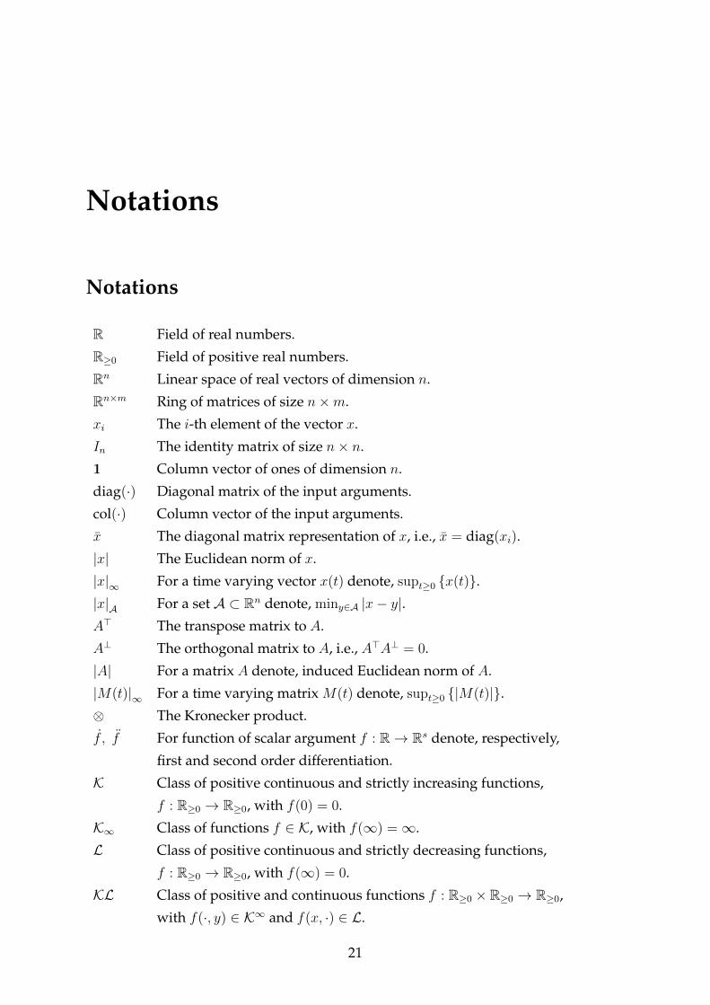
Notations
R Field of real numbers.
R≥0 Field of positive real numbers.
Rn Linear space of real vectors of dimension n.
Rn×m Ring of matrices of size n×m.
xi The i-th element of the vector x.
In The identity matrix of size n× n.
1 Column vector of ones of dimension n.
diag(·) Diagonal matrix of the input arguments.
col(·) Column vector of the input arguments.
x The diagonal matrix representation of x, i.e., x = diag(xi).
|x| The Euclidean norm of x.
|x|∞ For a time varying vector x(t) denote, supt≥0 x(t).|x|A For a set A ⊂ Rn denote, miny∈A |x− y|.A> The transpose matrix to A.
A⊥ The orthogonal matrix to A, i.e., A>A⊥ = 0.
|A| For a matrix A denote, induced Euclidean norm of A.
|M(t)|∞ For a time varying matrix M(t) denote, supt≥0 |M(t)|.⊗ The Kronecker product.
f , f For function of scalar argument f : R→ Rs denote, respectively,
first and second order differentiation.
K Class of positive continuous and strictly increasing functions,
f : R≥0 → R≥0, with f(0) = 0.
K∞ Class of functions f ∈ K, with f(∞) =∞.
L Class of positive continuous and strictly decreasing functions,
f : R≥0 → R≥0, with f(∞) = 0.
KL Class of positive and continuous functions f : R≥0 × R≥0 → R≥0,
with f(·, y) ∈ K∞ and f(x, ·) ∈ L.
21

22
Lp The space of p(> 0) integrable functions, f : R≥0 → Rn ∈ Lp⇒[∫∞
0|f(s)|p ds
] 1p <∞.
xt For x : R≥0 → Rn, denote the functional xt(θ) := xt(t+ θ), for all θ ∈ [−T, 0].
C[−T, 0] The space of functions which are continuous on [−T, 0].
|xt|A For a functional xt ∈ C[−T, 0] denote, maxθ∈[−T,0] |x(t+ θ)|A.
W [−T, 0] The space of functions which are absolutely continuous on [−T, 0],
and have square integrable first order derivatives.
‖xt‖A For a functional xt ∈ W [−T, 0] denote,
maxθ∈[−T,0] |x(t+ θ)|A + [∫ 0
−T |x(t+ s)|2 ds]1/2.
L2[−T, 0] The space of square integrable functions on [−T, 0].
For a symmetric positive semi-definite matrix L ∈ Rn×n, we define
λM(L) The maximum eigenvalue of L.
λm(L) The minimum eigenvalue of L.
λi(L) The ith eigenvalue of L greater then λm(L).
Acronyms
a.e. Almost Everywhere
PE Persistently Exciting
US Uniformly Stable
UAS Uniformly Asymptotically Stable
UES Uniformly Exponentially Stable
UGAS Uniformly Globally Asymptotically Stable
UGES Uniformly Globally Exponentially Stable
ISS Input-to-State Stability
iISS integral Input-to-State Stability
PD Proportional and Derivative
PI Proportional and Integral
PID Proportional, Integral and Derivative
SLF Strict Lyapunov Function
SLKF Strict Lyapunov Krasovskii Functional

Chapter 1
Strict Lyapunov functions for
time-varying systems with persistency
of excitation
Establishing uniform asymptotic stability of the origin for time-varying systems is a
difficult task in general, even for linear systems. For instance, for the latter, eigen-
value analysis is generally inconclusive, even for boundedness of the solutions. Much
of the control literature in which time-varying systems appear, relies on generic meth-
ods of proof that are based on “signal chasing” arguments such as Barbalat’s lemma,
properties of functions in Lp spaces, etc. In general, finding a strict Lyapunov func-
tion (that is, which is positive definite, radially unbounded and with negative definite
derivative) is an extremely challenging problem.
The notion of persistency of excitation, which was originally introduced in the con-
text of systems identification [11], is known to be necessary and sufficient for uniform
exponential stability of certain linear time-varying systems [82]. Early proofs of such
statement rely on concepts such as uniform complete observability [83], output injec-
tion arguments [7] and other (rather intricate) methods tailored specifically for linear
systems [41].
In so-called model-reference adaptive control [86], persistency of excitation plays a
fundamental role as a necessary and sufficient condition for uniform global asymptotic
stability. For functions that depend on the state and time, however, persistency of
excitation must be redefined and the stability anaysis demands a special treatment.
For instance, on occasions it appears convenient to analyse nonlinear time-varying
systems as linear time-varying [47, p. 659]. Such method of analysis renders possible
the extension of stability tools devoted to linear time-varying systems with persistency
of excitation, to the realm of nonlinear systems [63]. Nevertheless, as it is showed in
23

24
the latter reference, it is fundamental to take special care in imposing a uniform variant
of persistency of excitation, independent of the initial conditions.
More recently, new notions of peristency of excitation tailored to establish uniform
attractivity for nonlinear time-varying systems, were introduced in [50, 51, 66, 99]. In
the first two, links between persistence of excitation and detectability are established.
In the latter two, necessary and sufficient conditions for uniform global asymptotic
stability of generic nonlinear time-varying systems are given.
Beyond stability analysis, persistency of excitation plays a fundamental role in con-
trol design, as for instance, in systems in which the control input is multiplied by a
time-varying function –see [61]. Such is the case of certain systems in aerospace engi-
neering applications –see e.g., [113], [4], and [69].
Persistency of excitation appears naturally in control design when there is a struc-
tural impediment to use autonomous smooth feedback, as in the case of chain-form
systems [64, 108]. In [108], under a change of coordinates and a preliminary feed-
back, the closed-loop system is transformed into a so-called skew-symmetric system,
roughly of the form x = Ax + Bu with u ∈ R where A ∈ Rn×n is diagonal with only
one element different from zero andB ∈ Rn×n is skew-symmetric. Then, following the
design rationale from [108], in [64] uniform global asymptotic stability was established
for the closed-loop systems using controllers with persistency of excitation. Other con-
trol applications include the stabilization of parameterized time-varying systems [116]
and the analysis and design of observers for bilinear systems [14, 123].
As we shall show here, persistency of excitation also provides a naturally relaxed
condition for the solution to the so-called consensus problem [105] for systems with
time-varying interconnections. In this scenario, stating conditions of persistency of
excitation on the communication channels is particularly useful to characterize the
“minimal reliability” of the channels [115]. In much of the existing literature, how-
ever, the study of consensus under time-varying communication links makes use of
trajectory based approaches by means of a non differentiable Lyapunov functions to es-
tablish the contraction of trajectories. See for instance the seminal work of Moreau [79]
in which the communication signals take a arbitrarily positive values. Similar prob-
lems are treated, for example, in [37] and [38] under relatively relaxed conditions on
communication signals and on the graph topologies.
Furthermore, on top of stability and stabilisation one must also recognize the ques-
tion of performance. Specifically, to determine explicit exponential estimates that relate
the property of persistency of excitation to the overshoot and convergence rates. For
the so-called “gradient” systems explicit bounds were independently provided in [16]
and [63]. For more complex cases, such as that of model-reference adaptive control

Chapter 1 25
systems see [58]. It is to be noted, however, that the methods of proof in these refer-
ences are rather intricate since they do not rely on the construction of strict Lyapunov
functions.
In this first chapter we present the technical basis for the presentation of our contri-
butions in the subsequent chapters. We broach several case-studies of stability analysis
of time-varying systems:
• cascaded systems [97],
• consensus under spanning tree topology and time-varying communication links
[105],
• model-reference adaptive control [88],
• stabilization of non-holonomic systems [108],
• systems with time-varying input gain [19, 61].
For all these case-studies we establish statements of uniform global exponential sta-
bility via Lyapunov’s direct method. For each of these we give concrete examples in
which our results are useful. From a technical viewpoint, the design of our Lyapunov
functions is mostly inspired by [74] but we also use the results in [76] and [72], mainly
for the strictification of Lyapunov functions with a non-positive persistently-exciting
bounds on the time-derivatives.
Each of the case studies broached here is representative of a wide research area
hence, we do not develop them in depth. In the subsequent chapters we present part
of the work we accomplished in the period of this thesis (36 months). For clarity of
exposition we chose to focus on problems of stabilization and formation control (con-
sensus) of autonomous vehicles.
1.1 Case-study: a comparison positive system
We start with a simple statement that, in addition to setting the basis for our results, is
interesting in its own right. Consider the differential equation
v = −q(t)v, v ∈ R (1.1)
where q : R≥0 → R≥0. Invoking standard results on adaptive control – see e.g., [41], one
may conclude that the origin is UGES if and only if√q is continuous and persistently
exciting, see Definition A.6, that is, if there exist T , µ > 0 such that∫ t+T
t
q(s)ds > µ ∀ t ≥ 0. (1.2)

26
Here, we establish the same result, by providing a strict Lyapunov function. The
construction method for this and all other Lyapunov functions in this memoir is in-
spired from [72, 75]. It relies on a functional that is defined upon a locally Lipschitz
bounded persistently exciting function ψ : R≥0 → R≥0 with bounded first derivative
(a.e.), that is, we assume that there exists a constant ψ > 0, such that
max|ψ(t)|∞, |ψ(t)|∞
≤ ψ a.e. (1.3)
Then, we define the functional Υ : (R≥0 → R≥0)→ R, such that, for all ψ : R≥0 → R≥0
Υψ(t) := 1 + 2ψT − 2
T
∫ t+T
t
∫ m
t
ψ(s)ds dm (1.4)
and, for further development, we remark that this function is lower and upper bounded,
in particular,
1 ≤ Υψ(t) < Υψ := 1 + 2ψT. (1.5)
Furthermore, after the fundamental theorem of calculus, the derivative of this function
has the form
Υψ(t) = − 2
T
∫ t+T
t
ψ(s)ds+ 2ψ(t) (1.6)
then, using persistency of excitation of the signal√ψ(t), we can upperbound the
derivative of Υψ as
Υψ(t) ≤ −2µ
T+ 2ψ(t). (1.7)
Remark 1.1. The function
p(t) :=− 2
T
∫ t+T
t
∫ m
t
ψ(s)ds dm (1.8)
was first introduced in [74] under the equivalent form
p(t) =
∫ t+T
t
(s− t− T ) q(s)ds, (1.9)
which is obtained by simple change of the order of integration.
The following statement presents a strict Lyapunov function which establishes this,
otherwise well-known, result –cf. [60].
Lemma 1.1. Let q : R≥0 → R≥0 be essentially bounded and let inequality (1.2) hold. Under
these conditions, for the system (1.1), the function W : R≥0 × R→ R≥0, defined by
W (t, v) =1
2Υq(t)v
2 (1.10)
Chapter 1 27
is a strict Lyapunov function and the origin v = 0 is uniformly globally exponentially stable.
Proof. Let q be such that |q(t)| ≤ q for all t ≥ t0 and define pM := qT . defining the
function p(t) using (1.8), we obtain that q(t) ≥ 0, −pM ≤ p(t) ≤ 0, and |p(t)| ≤ pM for
all t ≥ 0 hence, W (t, v) can be bounded as
1
2v2 ≤ W (t, v) ≤
[12
+ qT]v2. (1.11)
The derivative of W along the trajectories of (1.1) yields
W (t, v) = −[q(t)Υq(t)−
Υp
2
]v2,
then using (1.5) and (1.6) we obtain
W ≤ −[
1
T
∫ t+T
t
q(s)ds
]v2 ∀t ≥ 0 (1.12)
and, in view of (1.2), we obtain that for all t ≥ t0 and v ∈ R
W (t, v) ≤ −µTv2. (1.13)
Finally, using (1.11), we also have
W (t, v) ≤ − 2µ
(1 + 2qT )TW (t, v) (1.14)
which, by integrating along the trajectories, yields
|v(t)| ≤√
1 + 2qT |v(t)|exp[− µ(t− t)
(1 + 2qT )T
]∀t ≥ t0. (1.15)
Remark 1.2. The requirement that q(t) ≥ 0 is not necessary —see [60, Lemma 1], that is,
under an extra condition on the excitation parameters (T, µ), one can establish UGES of (1.1)
under (1.2) without requiring q(t) to be positive. For example, one possible way to derive the
extra condition on the parameters (T, µ) is to decompose q(t) as q(t) := q1(t) + q2(t) where
q1(t) ≥ 0 verifies (1.9) and q2(t) is bounded, then using the Lyapunov function provided in
(1.10), in which we replace q(t) by q1(t), one can easily derive a sufficient condition, that relies
the excitation parameters (T, µ) to the upper bounds of both q1(t) and q2(t), such that the
time-derivative of (1.10), along trajectories of (1.1), is negative definite.
The simplicity of Lemma 1.1 should not eclipse its utility in stability analysis. For
28
instance, along with the comparison lemma [47, Lemma 2.5], it may be used to es-
tablish uniform global asymptotic stability, with guaranteed convergence rates, for
certain nonlinear time-varying systems. To see this, consider the equation
z = f(t, z) (1.16)
and let V : R≥0×Rn → R≥0 be positive definite, proper and decrescent, that is, assume
that there exist α1, α2 ∈ K∞ such that
α1(|z|) ≤ V (t, z) ≤ α2(|z|). (1.17)
Assume, further, that there exists a globally Lipschitz continuous function q : R≥0 →R≥0, satisfying (1.2),
V (t, z) ≤ −q(t)V (t, z). (1.18)
Then, let us define v(t) := V (t, z(t)), so that v(t) ≤ −q(t)v(t) for all t ≥ 0. In view
of the monotonicity properties of V and the comparison lemma, Lemma 1.1 directly
establishes UGAS of the origin, z = 0, with an explicit decay estimate. Indeed, from
(1.15), (1.17) and the comparison Lemma, we obtain
|z(t)| ≤ α−11
(kvα2(|z|)e−λv(t−t)
)(1.19a)
λv :=µ
k2vT, kv :=
√1 + 2qT . (1.19b)
Example: Nonlinear observer design
To illustrate further the utility of Lemma 1.1, consider the problem of designing an
observer for a bilinear system
x = A(u, y)x+B(u, y) (1.20a)
y = C(u, y)x. (1.20b)
Since the system is linear in the unmeasured variable, we may proceed with a ”Luenberger-
like” design. To that end, let x denote the state estimate and let us define its dynamics
through the equation
˙x = A(u, y)x+B(u, y)− L(u, y)C(u, y)[x− x] (1.21)
where the observer gain, L, is to be designed in order to ensure that the origin of the
estimation-errors system is UGES.

Chapter 1 29
Proposition 1.1. Consider the system (1.20) and the observer (1.21). Let L be continuous, and
let u, y be such that there exist a continuously-differentiable function P : R≥0 ×Rn → R≥0, a
continuous function qm : R≥0 → R≥0 and positive constants pm, pM , µ and T such that:
(i) defining A(t) := A(u(t), y(t)) − L(u(t), y(t))C(u(t), y(t)) and Q(t) := −P (t) −P (t)A(t)−A(t)>P (t), we have
Q(t) ≥ qm(t)I ≥ 0 ∀ t ≥ 0;
(ii) √qm is persistently exciting uniformly in y(t) and u(t) i.e., it satisfies (1.2) with µ and
T independent of the initial conditions1;
(iii) the matrix P (t) is uniformly positive definite and bounded, i.e.,
pmI ≤ P (t) ≤ pMI.
Then, the estimation errors z(t) satisfy the bound
|z(t)| ≤ kv
√pMpm|z|e−λv(t−t) (1.22)
where kv and λv are defined in (1.19b).
Proof. Let the estimation errors be defined as z := x− x hence,
z = A(t)z. (1.23)
Then, consider the function V : R≥0 × Rn → R≥0 defined by V (t, z) := z>P (t)z. This
function satisfies (1.17) with α1(s) := pms2 and α2(s) := pMs
2. Moreover, defining
q(t) := qm(t)pM
, a direct computation shows that the time-derivative of V along the trajec-
tories of (1.23) satisfies (1.18). Therefore, by Lemma 1.1, we see that
W(t, z) :=1
2Υq(t)[z
>P (t)z]2
is a Lyapunov function for the estimation error dynamics (1.23) and, moreover, (1.19a)
holds which, in this case, is equivalent to (1.22).
The statement of Proposition 1.1 generalizes some results that rely on a uniform
1See [63] for details.

30
complete observability condition, e.g., the choice:
P = −εP −[A(u, y)>P + PA(u, y)] + 2C>C (1.24a)
L := P−1C>, P (t) ≥ pmI, (1.24b)
commonly used in observer design for bilinear systems –cf. [14], guarantees that P (t),
hence Q(t) := εP (t), is positive definite and bounded, for all t ≥ T . The persistency of
excitation condition onQ, imposed in Proposition 1.1, is less restrictive than positivity;
moreover, the gain L(t) as defined in (1.24b) may reach very high values [14]. Yet, the
advantage of this choice is that it leads directly to an exponential-convergence estimate
and provides a strict Lyapunov function for the estimation error-system. That is, this
construction naturally lends itself for output-feedback high-gain designs, notably for
systems with Lipschitz non-linearities –see e.g., [2]. On the other hand, for such type
of systems, notably chaotic oscillators, the main result in [68] provides an observer of
the type of (1.21), under the less restrictive persistency of excitation condition on Q(t).
Thus, the statement of Proposition 1.1 covers all the previously mentioned results by
providing an explicit stability bound under the weaker condition of persistency of
excitation.
1.2 Case-study: Cascaded systems
We extend the result in Lemma 1.1 by establishing a statement of stability for linear
cascaded systems that are persistently excited. We broach two case-studies: first, that
of a chain of single integrators and, second, a more general case of multivariable sys-
tems.
1.2.1 Chain of single integrators
For the sake of illustration, let us start with the 2nd-order system:
x1 = −a1(t)x1 + a12(t)x2 (1.25a)
x2 = −a2(t)x2 (1.25b)
under the assumption that a1, a2 and a12 are continuous, uniformly bounded functions,
and a1, a2 non negative having persistently exciting square root.
For this system, exponential stability of the origin x1 = x2 = 0 may be assessed
following a direct cascades argument. Indeed, this follows, e.g., from the results in [97]
Chapter 1 31
observing that, by Lemma 1.1, the respective origins of
x1 = −a1(t)x1 x2 = −a2(t)x2 (1.26)
are UGES and a2(t) is bounded hence, the solutions x1(t) of equation (1.25a) are uni-
formly globally bounded. The statement also follows from the fact that (1.25a) is
ISS with Lyapunov function W (t, x1) defined by (1.10) and input x2. However, even
though the cascades argument is straightforward for the case of two interconnected
systems, the argument is hard to extend to cascades of n > 2 time-varying systems,
Σ′n :
x1 =− a1(t)x1 + a12(t)x2
x2 =− a2(t)x2 + a23(t)x3
...
xn−1 =− an−1(t)xn−1 + a(n−1)n(t)xn
xn =− an(t)xn,
(1.27)
relying purely on converse Lyapunov theorems. Our next statement removes this dif-
ficulty by providing a strict Lyapunov function.
Theorem 1.1. Consider the system (1.27) under the following hypotheses:
Assumption 1.1. (Non-negativity): ai(t) ≥ 0 for all i ≤ n and all t ≥ 0.
Assumption 1.2. (Boundedness): There exists a > 0 such that
max|ai(t)| ,
∣∣a(i−1)i(t)∣∣ ≤ a
for all t ≥ 0 and all i ≤ n.
Assumption 1.3. (Persistency of Excitation): There exist µ, T > 0 such that∫ t+T
t
ai(s)ds > µ ∀i ≤ n, ∀ t ≥ 0. (1.28)
Then, defining β1 := 1 and, for each i ≤ n,
βi :=4βi−1T
2
µ2
[(1 + 2aT ) a
]2, ∀i ≥ 2, (1.29)
the function Vn : R≥0 × Rn → R≥0, defined as
Vn(t, x) := x>P (t)x (1.30)

32
with
P (t) :=1
2diag (Υai(t)βi) ,
is a strict Lyapunov function, and
Vn(t, x) ≤ − µ
2TxTdiag (βi)x. (1.31)
Consequently, the origin is uniformly globally exponentially stable.
The proof is reported in Appendix B.1.
Remark 1.3. From the previous theorem it also follows that the trajectories of the system (1.27)
satisfy
|x(t)|2 ≤ αM |x|2e−(µ/2TαM )(t−t) ∀t ≥ t
where αM := 1 + (2T + βn)a. To see this, we observe that the Lyapunov function Vn(t, x)
satisfies (since βn > βn−1 > · · · β1 = 0)
(1/2)αM |x|2 ≥ Vn(t, x) ≥ (1/2)|x|2.
Example: consensus under spanning tree
To illustrate the utility of the case studied in Theorem 1.1, we consider a classical track-
ing consensus problem concerning n agents interconnected in a spanning-tree topol-
ogy with time-varying interconnection gains. In this case, each agent communicates
only with two neighbors. Even though here we consider that each agent communi-
cates always with the same neighbours, in general, this does not need to be the case
–cf. [6]. We limit our case-study to this topology because in concrete cases of formation
control, or follow-the-leader tracking control for that matter, using such communica-
tion topology excludes communication redundancy. This idea is pursued in Chapters
2-4 for the case of multiple nonholonomic mobile robots, where we are interested to
solve the leader-follower problem under different configurations of the leader’s veloc-
ities.
From a strictly theoretical viewpoint, however, our stability statement per se in this
section is covered by, e.g., [80]. On the other hand, as far as we know, we provide
for the first time a strict smooth Lyapunov function which, in turn, allows to establish
input-to-state stability (ISS) of the closed-loop system – see Appendix A.4.
Thus, let us consider n dynamical systems defined by
zi = fi(t, zi) + ui, zi ∈ Rm, i ≤ n (1.32)

Chapter 1 33
which are required to follow a reference trajectory z∗ : R≥0 → Rm generated by an
exogenous system z∗ := f ∗(t, z∗). We assume that only the controller for the last (n-th)
agent has access to the reference trajectory. Then, the ith agent receives information
from the i + 1st, thereby establishing a spanning-tree topology, albeit through unreli-
able channels.
To recast this consensus-tracking problem into a stabilization one we introduce the
error system with state variables xi := zi − zi+1 for all i ≤ n, with zn+1 := z∗ and
fn+1 := f ∗. That is,
xi = fi(t, xi + zi+1(t))− fi+1(t, zi+1(t)) + ui − ui+1 (1.33a)
xn = fn(t, xn + z∗(t))− f ∗(t, z∗(t)) + un. (1.33b)
With this change of coordinates, the consensus problem boils down to stabilizing the
origin x = 0, with x := [x1, · · · , xn]>, for the non-autonomous system (1.33). To do
so, we use the control inputs
ui := −γai(t)[zi − zi+1] + wi, ai(t) ≥ 0, ∀ t ≥ 0 (1.34)
where the functions ai are assumed to be bounded and persistently exciting, γ > 0 is
the interconnection strength, and wi denote “additional” inputs to be defined. Then,
the closed-loop system is
xi = −γai(t)xi + γai+1(t)xi+1 + ψi(t, xi) + vi (1.35a)
xn = −γan(t)xn + ψn(t, xn) + vn (1.35b)
with vi := wi − wi+1 and
ψi(t, xi, zi+1) := fi(t, xi + zi+1(t))− fi+1(t, zi+1(t)), i ≤ n. (1.36)
Note that the system (1.35) may be regarded as a “perturbed” version of (1.27) hence,
the following statement, which implies robust consensus-tracking of (1.32), follows as
a corollary of Theorem 1.1.
Lemma 1.2. Consider the system (1.35) under assumptions 1.1–1.3. For each i ≤ n, let vibe measurable functions, let ψi : R≥0 × Rm → Rm be such that there exist continuously-
differentiable class K∞ functions Li such that
|ψi(t, xi)| ≤ Li(|xi|). (1.37)

34
Let Ri be such that for all xi ∈ BRi , where BRi := xi ∈ R : |xi| ≤ Ri,∣∣∣∂Li∂s
(|xi|)∣∣∣ ≤ `i
and the interconnection strength γ is such that
µγ
2T> 2`i
[1 + a2T
].
Then, the system (1.35) is input-to-state-stable from the input v := [v1, · · · , vn]>, for all ini-
tial conditions t ≥ 0 and xi ∈ Rn which produce complete trajectories satisfying xi(t, t, xi) ∈BRi .
Sketch of proof:
Following the proof of Theorem 1.1 the Lyapunov function Vn defined in (1.30)
satisfies
Vn(t, x) ≤ −n∑i=1
[µγ2T− `i
[1 + a2T
] ]x2i +
[1 + a2T
]xivi (1.38)
for all xi ∈ BRi . Then, we see that inequality |vi| ≤ `i|xi| imply that
Vn(t, x) ≤ −n∑i=1
[µγ2T− 2`i
[1 + a2T
] ]x2i . (1.39)
Then, it follows that the function Vn defined in (1.30) is an ISS Lyapunov function
for all xi ∈ BRi and each i ≤ n. Hence, the system is input-to-state stable for all initial
conditions t ≥ 0, xi ∈ BRi generating complete trajectories that satisfy |xi(t, t, xi)| ≤Ri for all t ≥ t ≥ 0 and all i ≤ n.
1.2.2 Multivariable cascaded linear time-varying systems
Let us consider now, the cascade of multivariable linear-time-varying persistently-
excited systemsx1 =A1(t)x1 +B1(t)x2
...
xn−1 =An−1(t)xn−1 +Bn−1(t)xn
xn =An(t)xn, xi ∈ Rm,
(1.40)
where B(t) and A(t) : R≥0 → Rn×n are continuously differentiable, and the following
hypotheses hold:
Assumption 1.4. (Boundedness) There exists B > 0 such that |Bi|∞ ≤ B.
Chapter 1 35
Assumption 1.5. (Lyapunov Equation) There exist positive definite matrices Pi(t), positive
semi-definite matrices Qi(t), positive constants PiM , Pim and time-varying function qim :
R≥0 → R≥0, such that; for all t ≥ 0,
PimIn ≤ Pi(t) ≤ PiMIn (1.41)
0 ≤ qim(t)In ≤ Qi(t) (1.42)
Pi + A>i Pi + PiAi = −Qi(t) (1.43)
Assumption 1.6. (Persistency of excitation) There exists a positive constants µ, T , such that:∫ t+T
t
qim(s)ds > µ ∀t ≥ 0. (1.44)
This type of systems generalizes that of the single chain of integrators presented
previously. We have the following.
Theorem 1.2. Under assumptions 1.4, 1.5 and 1.6 there exists a quadratic strict differentiable
Lyapunov function for (1.40).
Proof. For each i ≤ n, let us define Vi(t, x) = x>i Pi(t)xi. The derivative of each Vi along
the trajectories of (1.40), satisfies
V1 ≤− x>1 Q1(t)x1 + 2x>1 P1B1(t)x2
...
Vn−1 ≤− x>n−1Qn−1(t)xn−1 + 2x>n−1Pn−1Bn−1(t)xn
Vn ≤− x>nQn(t)xn.
(1.45)
Then, consider the modified Lyapunov function Wi : R≥0 × Rnm → R≥0 defined by
Wi(t, x) = (Υqim(t) + 2PiM)Vi(t, x). Using (1.6) and (1.5) we obtain
W1 ≤−2µ
Tx>1 P1x1 + 2q1m(t)x>1 P1x1 − 2P1Mx
>1 Q1(t)x1 + 2 (Υq1m(t) + 2P1M)x>1 P1B1x2
...
Wn−1 ≤−2µ
Tx>n−1Pn−1xn−1 + 2qn−1m(t)x>n−1Pn−1xn−1 − 2Pn−1Mx
>n−1Qn−1(t)xn−1
+ 2(Υqn−1m(t) + 2Pn−1M
)x>n−1Pn−1Bn−1xn
Wn ≤−2µ
Tx>1 P1x1 + 2q1m(t)x>1 P1x1 − 2P1Mx
>1 Q1(t)x1
We define φi(t) := Υqim(t) + 2PiM , a nonsingular matrices νi : R≥0 → Rn×n such that
Pi(t) = νi(t)>νi(t) and Mi(t) = φi(t)νi(t)Biνi+1(t)−1. Then using Assumption 1.6, from

36
(1.45) we obtain that derivatives of the functions Wi(t, x) can be bounded as
W1 ≤−2µ
T|ν1x1|2 + 2(ν1x1)>M1(t)ν2(t)x2
...
Wn−1 ≤−2µ
T
∣∣ν>n−1xn−1
∣∣2 + 2(νn−1xn−1)>Mn−1(t)νn(t)xn
Wn ≤−2µ
T
∣∣ν>n xn∣∣2 .(1.46)
Using the inequality
2(νixi)>Miνi+1xi+1 ≤
µ
T|νixi|2 +
T
µ|Mi|2∞ |νi+1xi+1|2
to estimate cross terms in (1.46), we obtain the following bounds for the derivatives
W1 ≤−µ
T|ν1x1|2 +
T
µ|M1|2∞ |ν2x2|2
...
Wn−1 ≤−µ
T
∣∣ν>n−1xn−1
∣∣2 +T
µ|Mn−1|2∞ |νnxn|
2
Wn ≤−µ
T
∣∣ν>n xn∣∣2 .(1.47)
Finally, the strict Lyapunov function for the system (1.40) is given by
W(t, x) =n∑i=1
βiWi(t, xi)
where β1 = 1 and βi+1 = 2T 2
µ2 |Mi|2∞ βi, while its derivative satisfies the inequality
W(t, x) = −µT|ν1x1|2 −
n∑i=2
T
µβi−1 |Mi−1|∞ |νixi|
2 .
Example: master-slave synchronization
In order to illustrate the use of Theorem 1.2, let us consider the following case-study
of consensus-tracking control of Lagrangian systems,
Di(qi)qi + Ci(qi, qi)qi + gi(qi) = τi, τi, qi ∈ Rp. (1.48)
Chapter 1 37
The functions Di, Ci and gi are, respectively, the inertia matrix, the Coriolis matrix and
the potential forces vector. The control torques are denoted by τi.
We consider the problem of tracking and mutual synchronization —see [89] in
which all systems are required to follow a common exogenous trajectory t 7→ q∗. Now,
we assume that the systems are interconnected in a spanning-tree topology through
unreliable links hence, on intervals of time the nodes may be isolated.
First, to each system we apply the preliminary linearizing feedback (this is possible
because D is full rank) τi = Di(qi)ui + Ci(qi, qi)qi + gi(qi) so that the equation of each
node becomes qi = ui.
Then, emulating the unreliability of the communication channel by a square-pulse
function a : R≥0 → 0, a the control input becomes
ui = a(t)[−k1(qi − qi+1)− k2(qi − qi+1) + qi+1]
that is, the control is active only when a(t) = a > 0.
Now, for each i ≤ n, define xi := [q>i q>i ]> − [q>i+1 q>i+1]>. We see that the error
dynamics, in closed-loop, takes the form
xi = Ai(t)xi +Bi(t)xi+1 + vi(t), i ≤ n− 1
where the perturbation vi, which stems from the fact the “feedforward” term qi+1 in uiis not available all the time, is defined as vi(t) := [a(t)−1][qi+1(t)−qi+2(t)]. Furthermore,
Ai(t) :=
[0 1
−a(t)k1 −a(t)k2
], Bi(t) =
[0
a(t)
]
and, for i = n we have xn = An(t)xn + vn with vn(t) := [a(t)− 1]q∗(t).
By Theorem 1.2, for vi ≡ 0, the origin is uniformly exponentially stable and admits
a strict smooth Lyapunov function provided that Assumptions 1.4–1.6 hold. To verify
these assumptions, we follow the second construction in [61] for double integrators
with time-varying persistently-exciting input gain, x = α(t)u, and define
a(t) :=α(t)
α(t) + ε, ε ∈ (0, 1). (1.49)
In the current example we used k1 = k2 = 1 for all agents but, in general, different
gains may be used.
Following the reasoning proposed in [61], we decompose the matrices Ai (i =
1, ..., n− 1) as follows

38
Ai(t) = Ai0 +ε
ε+ α(t)Ai1, (1.50)
where
Ai0 :=
[0 1
−1 −1
], Ai1 :=
[0 0
1 1
].
We choose α(t) as a positive periodic pulse function of period T = 40s, with a duty
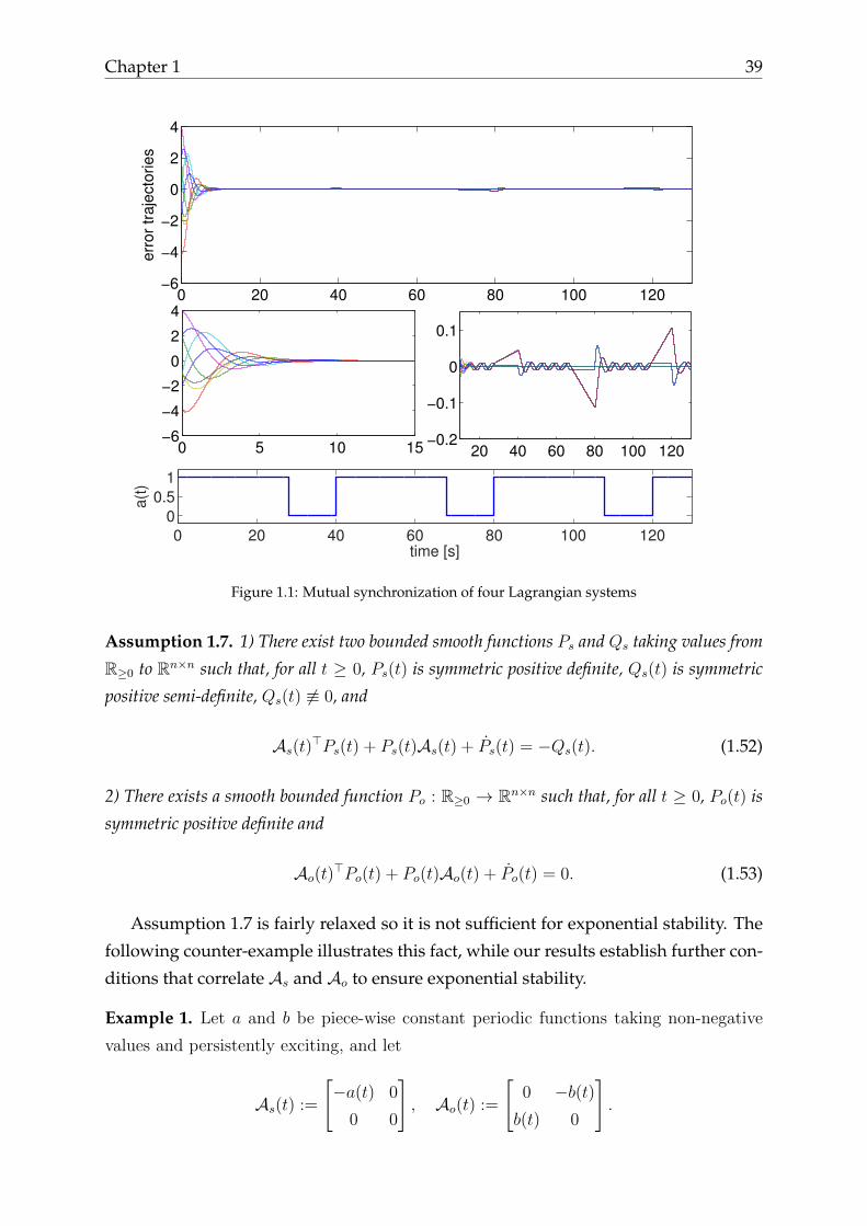
cycle of 70% and ε = 0.01. Hence, a(t) ≈ α(t) is also positive and√a(t) is persistently
exciting –see the bottom plot in Figure 1.1, thus the assumptions 1.1–1.3 hold.
The ”nominal” dynamics xi = Ai(t)xi has been studied in [61, Proposition 2]. In
our case, if we takeQi := 0.16255 I2, then there exists Pi ∈ R2 constant positive definite
such that
ATi0Pi + PiAi0 = −Qi,
and
ATi (t)Pi + PiAi(t) = −qim(t)I2.
with qim(t) ≥ 0 and qim(t) ≈ a(t). So we can see that Assumptions 1.5 and 1.6 hold for
this particular choice of α(t). Using Theorem 1.2, with vi(t) ≡ 0, we conclude UGES
hence, formation tracking control of (1.48). Input-to-state stability with respect to the
disturbance vi also may be concluded. Simulation results are presented in Figure 1.1,
for the case when all systems follow the reference trajectory q∗(t) = sin(t). The steady-
state error depicted in the zoomed portion of the figure illustrates the ISS statement.
1.3 Case-study: spiraling systems
In this second part, we address the question of stability for linear time-varying systems
of the general form
x = [Ao(t) +As(t)]x, x ∈ Rn (1.51)
where Ao and As are bounded differentiable mappings R≥0 → Rn×n. The model (1.51)
has two essential constituting parts: the so-called oscillating drift Ao(t)x and the steer-
ing drift As(t)x. In words, it is assumed that under the action of the former, the trajec-
tories of (1.51) tend to oscillate while under the action of the latter, there exists a van-
ishing output y := C(t)>x. Under a detectability argument, provided by persistency of
excitation, the trajectories tend to the origin while describing attenuated oscillations.
Hence the name of spiraling systems.
To characterize the steering and oscillating properties of the system’s dynamics
we”’ introduce the following assumption
Chapter 1 39
0 20 40 60 80 100 120−6
−4
−2
0
2
4
err
or
traje
cto
ries
0 20 40 60 80 100 120
0
0.5
1
time [s]
a(t
)
20 40 60 80 100 120−0.2
−0.1
0
0.1
0 5 10 15−6
−4
−2
0
2
4
Figure 1.1: Mutual synchronization of four Lagrangian systems
Assumption 1.7. 1) There exist two bounded smooth functions Ps and Qs taking values from
R≥0 to Rn×n such that, for all t ≥ 0, Ps(t) is symmetric positive definite, Qs(t) is symmetric
positive semi-definite, Qs(t) 6≡ 0, and
As(t)>Ps(t) + Ps(t)As(t) + Ps(t) = −Qs(t). (1.52)
2) There exists a smooth bounded function Po : R≥0 → Rn×n such that, for all t ≥ 0, Po(t) is
symmetric positive definite and
Ao(t)>Po(t) + Po(t)Ao(t) + Po(t) = 0. (1.53)
Assumption 1.7 is fairly relaxed so it is not sufficient for exponential stability. The
following counter-example illustrates this fact, while our results establish further con-
ditions that correlate As and Ao to ensure exponential stability.
Example 1. Let a and b be piece-wise constant periodic functions taking non-negative
values and persistently exciting, and let
As(t) :=
[−a(t) 0
0 0
], Ao(t) :=
[0 −b(t)b(t) 0
].

40
For each integer n ≥ 0, let Jn := (π/b)[2n+ 1, 2n+ 2]. Then, for all t ∈ Jn, let a(t) := a
and b(t) := 0 while for all t 6∈ Jn we have a(t) := 0 and b(t) := b. Hence, a(t)b(t) ≡ 0
and the trajectories generated by (1.51) satisfy the dynamics of a system whose dynamics
switches between Σa and Σb, defined as
Σa :
x1(t) =− bx2(t)
x2(t) = bx1(t),∀ t 6∈ Jn
Σb :
x1(t) =− ax1(t)
x2(t) = 0∀ t ∈ Jn.
This system satisfies Assumption 1.7 with Po = Ps = I2 and Qs(t) =
[a(t) 0
0 0
]and yet,
the analytic computation of its solutions, from the initial condition (x1, x2) = (0,−1)
shows that they do not converge. Indeed, for all t ∈ [0, π/b] the mode Σa is active, which
yields to (x1(t), x2(t)) = (sin(bt),− cos(bt)) for all t ∈ [0, π/b]. At t0 := π/b the system
switches to the mode Σb with the initial condition (x1(t0), x2(t0)) = (0, 1), the trajectories
remain constants for all t ∈ J0. by induction we can see that for all tn := (π/b)(2n+1) (tn
the initial time of each sequence Jn) we have (x1(tn), x2(tn)) = (0,±1) and the trajectories
remain constants along all the interval Jn.
Thus, additional assumptions, relating properties of the matrices Po and Ps, should
be imposed to ensure exponential stability of the origin. Below we present two re-
sults that address two case studies of spiraling systems and we present some technical
results that cover the state of the art in this topic.
1.3.1 Case-study: “adaptive control” systems
First, let us consider the case where matrix As(t) is constant, while the matrix Ao(t)is skew-symmetric. This type of systems appears in the analysis of adaptive control
systems, for example, we recover the class of systems studied in [82]. If, in particular,
Ao ≡ 0 and As(t) is negative semidefinite we recover the systems studied in [83].
A particular case of the latter are “gradient-type” adaptive systems, defined as x =
−φ(t)φ(t)>x, for which it is well known that persistency of excitation of φ is necessary
and sufficient for uniform exponential stability [83]. There are various distinct proofs
of this fact in the literature –see e.g. [16,63]; as far as we know, the first strict Lyapunov
function was provided recently in [20].

Chapter 1 41
More generally, the system (1.51) also includes the familiar equation [41, 47, 88][e˙θ
]=
[A 0
0 0
]︸ ︷︷ ︸As
[e
θ
]+
[0 −B(t)
C(t) 0
]︸ ︷︷ ︸
Ao
[e
θ
](1.54)
for which there exists P = P> > 0 such that A>P + PA < 0 (i.e., A is Hurwitz)
and C(t) := B(t)>P . In this case, Assumption 1.7 holds with Po = Ps := diag(P, I).
For such systems, which appear in the context of model-reference adaptive control (in
which case e represents tracking errors and θ estimation errors), it is well known that
if in addition B(t) is bounded with a bounded derivative, and B(t) is also persistently
exciting, the origin is uniformly exponentially stable.
Stability analysis for this adaptive control schame can be found in numerous text-
books and research monographs, see for instance [41, 47, 88]. However, the first strict
Lyapunov function for model-reference adaptive control systems was provided only
recently in [75] —see also [74]. More precisely, in this reference vectors B and C co-
incide, i.e. B(t) = C(t) and depend both on time and the state, and A := A(x1) sat-
isfies x>1 A(x1)x1 ≥ c|x1|2 for some c > 0. Our first result (Theorem 1.3) provides a
strict Lyapunov function for the case in which As in (1.54) is time-varying and satis-
fies Lyapunov equation (1.52) hence, we relax the uniform-positivity condition on A
imposed [75]. The method consists in constructing a strict Lyapunov function starting
from a non strict one that satisfies V (t, x) ≤ −q(t)V (t, x) —cf. Section 1.1.
In particular, consider the system x1 =− A(t)x1 −B(t)>x2, x1 ∈ Rn
x2 = C(t)x1, x2 ∈ Rm(1.55)
where matrices A(t) and B(t) are uniformly bounded and have uniformly bounded
derivatives (a.e.).
The following result not only ensures exponential stability of this system but also
gives a strict Lyapunov function.
Theorem 1.3. For the system (1.55) assume that B ∈ C1 and there exists a positive definite
matrix function P ∈ C1 and positive semi-definite bounded matrix function Q ∈ C1, such

42
that
PmI ≤ P (t) ≤ PMI (1.56)
P (t)− A(t)>P (t)− P (t)A(t) = −Q(t)
C(t) = B(t)P (t).
In addition, assume that the function ψ : R≥0 → R≥0 defined by
ψ(t) := λm(Q(t))√λm(B(t)B(t)>),
where λm denotes the smallest eigenvalue, is persistently exciting and satisfies (1.3). Then,
the null solution of (1.55) is uniformly exponentially stable and the system admits the strict
Lyapunov function
V (t, x) = λ2m(Q(t))x1B(t)>x2 +
1
2
[Υψ2(t) + α
] [x>1 P (t)x1 + |x2|2
]with
α ≥ (2T/µ)λ3m(Q)|B|2∞ + (8T/µ)λm(Q)λ2
m(Q) |B|2∞ + (2T/µ)λ3m(Q)|A>B>|2∞
+ λ2m(Q)|B>|∞(1 + 1/Pm) + 2λm(Q)λm(BB>)PM + 2λm(Q)
∣∣B>C∣∣∞ . (1.57)
Indeed, we have
V (t, x) ≤ −(µ/4T )[x>1 Px1 + |x2|2
].
Proof. In view of (1.5), the boundedness of B, Q, and P , as well as (1.57), V is positive
definite and radially unbounded. Indeed,
V (t, x) ≥ (α + 1)
2
[λm(P ) |x1|2 + |x2|2
]− 1
2λ2m(Q(t)) |B(t)|∞
[|x1|2 + |x2|2
]≥ 1
2
[λm(P ) |x1|2 + |x2|2
](1.58)
and
V (t, x) ≤[Υψ2 + α
] [λm(P ) |x1|2 + |x2|2
]+ λ2
m(Q(t)) |B|∞[|x1|2 + |x2|2
](1.59)
we conclude using (1.57) that there exist η1, η2 > 0 such that
η1 |x|2 ≤ V (t, x) ≤ η2 |x|2 , x = [x>1 x>2 ]>.
Chapter 1 43
The time-derivative of V along trajectories of (1.55) yields
V (t, x) = 2λm(Q)λm(Q)x>1 B>x2 − λ2
m(Q)x>1 A>B>x2 − λ2
m(Q)x>2 BB>x2
+λ2m(Q)x>1 B
>Cx1 + λ2m(Q)x>1 B
>x2 −α
2x>1 Qx1
−µT
[x>1 Px1 + |x2|2
]+ ψ2
[x>1 Px1 + |x2|2
]≤ −α
2λm(Q) |x1|2 + λ2
m(Q)λm(BB>)x>1 Px1 + λ2m(Q)x>1 B
>Cx1
−λ2m(Q)x>1 A
>B>x2 + 2λm(Q)λm(Q)x>1 B>x2 + λ2
m(Q)x>1 B>x2
−µT|x2|2 −
µ
Tx>1 Px1. (1.60)
Then, we use the inequalities
λ2m(Q)x>1 B
>x2 ≤ε
2λ4m(Q)|B|2∞ |x1|2 +
1
2ε|x2|2 ,
2λm(Q)λm(Q)x>1 B>x2 ≤ 2ελ2
m(Q)λ2m(Q) |B|2∞ |x1|2 +
1
2ε|x2|2 ,
λ2m(Q)x>1 A
>B>x2 ≤ε
2λ4m(Q)
∣∣A>B>∣∣2∞ |x1|2 +1
2ε|x2|2 ,
which hold for any ε > 0. Hence, setting ε = 2T/µ and in view of (1.57), it follows that
V ≤ −(µ/4T )|x2|2 − (µ/T )x>1 Px1.
In the particular case of planar systems, i.e. x1, x2 ∈ R, Theorem 1.3 reduces to the
following statement, which plays a key role in robustness analysis of the closed-loop
systems considered in the next chapters.
Corollary 1.1. Consider the system x1 =− a(t)x1 − b(t)x2, a(t) ≥ 0
x2 = b(t)x1,(1.61)
Then, provided that a and b satisfy (1.3) with a and b respectively. Assume, in addition, that
ψ := ab is persistently exciting. Then, the function V : R≥0 × R2 → R≥0, defined as
V (t, x) = a(t)2b(t)x1x2 +1
2
[Υa2b2(t) + α
][x2
1 + x22]
44
with
α ≥ 2ab2
[1 +
a2T
4µ(3 + a)2
](1.62)
satisfies
V (t, x) ≤ −(µ/2T )[x2
1 + x22
].
Example: Master-slave synchronization
In order to illustrate the utility of Theorem 1.3, we consider a simple example treat-
ing the master-slave synchronization problem for two harmonic oscillators, the slave
system z = A(t)z +Bu and the master system z∗ = A(t)z∗, where
A(t) :=
[0 −ω(t)
ω(t) 0
], B =
[1
0
]
That is, both oscillators spin at the same variable frequency ω(t), but out of phase.
Then, the problem consists in ensuring that z(t) → z∗(t) exponentially fast under the
assumption that the oscillators are linked through an unreliable channel.
To solve this problem the control law is designed so that the closed-loop system
has the structure given by equation (1.51): a steering drift and an oscillating drift. The
latter is natural to the harmonic oscillators while the former may be added through
the simple static output feedback u = −a(t)[z1 − z∗1 ]. Indeed, note that the closed-loop
system has exactly the form (1.61) with x1 := z1 − z∗1 , x2 := z2 − z∗2 and b(t) := ω(t).
We conclude that phase-lock synchronization is achieved provided that a and ω are
bounded, have bounded derivatives, and their product is persistently exciting.
Remark 1.4. Note that the closed-loop system in this case is similar to that in Example 1
with b(t) = ω(t). Hence, we conclude that persistency of excitation of a(t), which ensures the
steering of x1 to zero, and that of ω(t), which contributes to propagate the stabilization effect of
a(t), does not suffice alone to ensure the attractivity of the origin. For the stabilization effect to
be properly propagated from one coordinate to another it is required that the product of a(t)ω(t)
is persistently exciting.
1.3.2 Case-study: “skew-symmetric” systems
The case study addressed in this final section is motivated by stabilization problems
where non-autonomous feedback are imposed by the control problem. These include:
leader-follower tracking control [53], stabilization of non-holonomic systems [64,108],
stabilization of systems with time-varying input gain [61, 113].

Chapter 1 45
We consider a particular class of systems defined by the following ordinary differ-
ential equation
x = −b(t)2BB>x+ a(t)Ax (1.63)
where matrix A ∈ Rn×n is neutrally stable, and matrix Ao(t) = a(t)A satisfies (1.53),
that is, there exists matrix Po ∈ Rn×n, constant positive definite, such that
Ao(t)TPo + PoAo(t) = 0,
the pair (A,B) is controllable, and both a(t) and b(t) are scalar functions defined on
R≥0, such that the product a(t)2b(t) is persistently exciting. It is easy to see that under
the imposed conditions, Assumption 1.7 holds with As(t) := −b(t)2BB> and Ps = In.
Equation (1.63) intersects with the class of systems studied in [82] and covers the
class of systems studied in [19], where uniform global exponential stability is ensured
for the particular case that a(t) ≡ 1 andA is skew-symmetric. More significantly, in the
latter reference the proof is trajectory-based whereas here, we give a strict Lyapunov
function (Theorem 1.4).
Notice that the so-called skew-symmetric systems [108] represent a particular case
of the system (1.63). Indeed, the seminal work [108] on stabilization of nonholonomic
systems in chain form:
z1 = u2
zi = u1zi−1
zm = u1,
where zi ∈ R, shows that using a suitable smooth global change of coordinates z 7→ x
and a preliminary feedback u2(t, z) in the new coordinates, the system may be written
as x1
x2
...
xm−1
=
−k1 −k2u1 · · · 0
u1 0. . . ...
... . . . . . . −km−1u1
0 · · · u1 0
x1
x2
...
xm−1
(1.64)
xm = u1. (1.65)
The term skew-symmetric was introduced in [108] motivated by the fact that the matrix
in (1.64) may be written as the sum ofAs :=diag[−k1 0 · · · 0], which satisfies (1.52) with
Ps = Im, and a neutrally stable (”skew-symmetric”) matrixAo that satisfies (1.53) with

46
Po :=diag [1, k2, k2k3, · · · ,∏m−1
i=2 ki]. Alternatively, (1.64) falls in the model (1.63)
with B = [1, 0 · · · 0], b ≡√k1, and a(t) := u1(t, z(t)). Now, following the rationale
of [108] where non-uniform global asymptotic stability is proved, in [64] it is shown
that under certain persistency of excitation assumption on the control input u1, the
origin of the system (1.64) is uniformly globally asymptotically stable. The proof is
based on [63] and exploits the equation (1.64) as a linear-time-varying system obtained
by replacing the nonlinear function u1(t, z) with a parametrized, by initial conditions,
time signal u1(t, z(t)) —see the discussion in the Introduction. However, such proof
is very involved as it appeals to a recursive output-injection argument. Our approach
allows to construct a strict Lyapunov function for this system and provide a direct
proof.
Theorem 1.4. Consider the system (1.63). Let us assume that the functions a(·), b(·) and their
derivatives are bounded, i.e., there exists a and b such that (1.3) holds, and ψ(t) := a(t)b(t)
is persistently exciting. In addition, assume that the pair (A,B) is controllable and that there
exist a constant positive definite matrix P = P> ∈ Rn×n, such that:
pmIn ≤ P ≤ pMIn (1.66a)
A>P + PA = 0, (1.66b)
PBB> = BB>P := CC>. (1.66c)
Define V : R≥0 × Rn → R≥0 as
V (t, x) :=1
2[γ + Υa4b2(t)]x>Px+ b(t)2a(t)3x>PA
n∑i=1
βiΓiPx (1.67)
where γ := γ1 + γ2,
γ1 :=T b6a6
2µPm
∣∣∣∣∣n∑i=1
βiC>
i∑j=1
[AΓiP − ΓiPA]
∣∣∣∣∣2
(1.68)
γ2 :=T a4
µPm
n∑i=1
βi∣∣M>PC
∣∣2∞ + b2a3
∣∣∣∣∣P 1/2An∑i=1
βiΓiP1/2
∣∣∣∣∣ , (1.69)
Γi :=i∑
j=1
Aj−1BB>Aj−1>. (1.70)
Under controlability of (A,B), the matrix P 1/2AΓnA>P 1/2 is non singular, and we take βnI ≥
[P 1/2AΓnA>P 1/2]−1 and constants βi are defined in reverse order, i.e., for each i ∈ n −

Chapter 1 47
1, · · · , 1,
βi ≥2nT
µPm
∣∣∣[PAiB]>M ∣∣∣2[ n∑k=i+1
βk
]2
−n−1∑k=i+1
βk (1.71)
where M =[2ba + 3ba
]A + ba2A2. Then, the function V is a strict differentiable Lyapunov
function for the system (1.63) and its origin is uniformly exponentially stable.
The proof is reported in Appendix B.2.
Remark 1.5. The strict Lyapunov function provided in Theorem 1.4 serves the corestone for
the analysis approach proposed in Chapter 2. the construction of Lyapunov function for a skew-
symmetric nonlinear time-varying systems in Proposition 2.1, and to establish some robustness
results with respect to external perturbations.
The following proposition extends Corollary 1.1 and, to some extent, Theorem 1.4
to a case of “skew-symmetric” systems, defined by (1.51), with
As := diag(−a1(t)2 0 · · · 0), (1.72a)
Ao(t) :=
0 −a2(t) 0 · · · 0
a2(t) 0 −a3(t) 0...
0 a3(t) 0. . . 0
... 0. . . . . . −an(t)
0 · · · 0 an(t) 0
. (1.72b)
The following statement also generalizes [63, Theorem 2] and provides a direct proof
for it, as opposed to the recursive output-injection argument used in this reference.
Proposition 1.2. Let the functions ai(t) satisfy the bound (1.3) with a. Assume in addition
that the function ψ := Πni=1ai(t), is persistently exciting, i.e., there exists T and µ > 0, such
that, ∫ t+T
t
ψ2(s)ds ≥ µ > 0, ∀t ≥ 0.
For each i ∈ [2, n] define xi := [x1 · · ·xi]> and
Φi(t, xi) =i∑
j=2
[aj
i∏k = 2k 6= j
a2k
]xj−1xj, i ∈ [2, n].
Then, provided that αi, for i = n down to i = 2, and γ satisfy the following:
αn = 1, αn−1 = a+4n(n− 1)2a2nT
µ(1.73)
48
αi = an−i +nT
µ
[ n∑j=i+1
a2jαj
][n∑
j=i+1
αj a2(j−i)
]+
[n∑
j=i+1
αj2ia(2j−1−i)
]2(1.74)
γ ≥ T
µ(a2 + 1)
( n∑i=2
αia2i−1
)2
+
(n∑i=2
2iαia2i−1
)2+
n∑i=2
αia2i−1
+2T a
µ
[n∑i=2
αia2i−1
]2
. (1.75)
We have that the function V : R≥0 × Rn → R≥0 defined as
V (t, x) =
[1
2Υψ2(t) + γ
]|x|2 + a2
1
[n∑i=2
αiΦi(t, xi)
]
is a strict differentiable Lyapunov function for (1.51), (1.72), and its derivative satisfies
V (t, x) ≤− µ
2T|x|2.
Consequently, the origin is uniformly globally exponentially stable.
The proof of the latter statement is presented in Appendix B.3.
Example: Control of underactuated ships
To illustrate the utility of Theorem 1.4, we briefly consider the tracking control problem
for underactuated ships that is solved in [53] under the assumption that the reference
trajectories are persistently exciting. For the purpose of this chapter, we remark that
the closed-loop system in this reference has the cascaded form
x1 =[As +Ao(t)
]x1 +G(t, x1, x2)x2, x1 ∈ R4 (1.76)
x2 = Fx2, x2 ∈ R2, (1.77)
where F ∈ R2×2 is a Hurwitz constant matrix, As ∈ R4×4 is a diagonal constant matrix
with two negative elements and two zero elements, matrix G(·) has linear growth in
x1 and Ao(t) depends on the reference trajectories and satisfies the second part of As-
sumption 1.7 –see [53] for details. Following standard arguments for cascaded systems
it is possible to establish uniform global asymptotic stability of the origin, provided
that the same property holds for the nominal system x1 =[As(t) + Ao(t)
]x1. In [53]
this is established under the assumption of persistency of excitation of the reference

Chapter 1 49
velocity along with uniform-complete-observability and output-injection arguments.
Theorem 1.4 not only delivers a strict Lyapunov function to ensure exponential stabil-
ity for the nominal x1–dynamics but it also constitutes a fundamental step to carry on
a robustness analysis with respect to unmodelled perturbations.
1.4 Conclusion
We have presented original strict Lyapunov functions for uniform exponential stability
of linear time-varying systems with persistency of excitation that appear in a variety
of problems including adaptive control systems, state estimation of bilinear systems,
consensus with persistently-exciting interconnections, master-slave synchronization,
etc. The utility of our theoretical findings is briefly demonstrated through concise but
representative examples of meaningful control problems.
In the succeeding chapters we present a deeper analysis of a particular area: that of
consensus and formation control of mobile robots, using controllers with persistency
of excitation. Although many of our controllers are reminiscent of others that have
appeared in the literature, our contributions lie in the establishment of strong proper-
ties such as uniform global asymptotic stability, (integral) intput-to-state stability and,
most remarkably, in the construction of original Lyapunov functions for most of the
control problems that we solve.
We believe that the construction of strict Lyapunov functions for nonlinear time-
varying systems with structures as those investigated here may lead to a range of
open problems in stability and control theory. Notably, the problem of establishing ro-
bustness properties (Input-to-output stability) is a well-motivated avenue of research
for which our statements might be a starting point.

50

Chapter 2
Leader-follower formation control of
nonholonomic vehicles
The landmark paper [46] introduced a follow-the-leader control approach for non-
holonomic mobile robots which translates a robotics problem into a standard stabi-
lization problem for time-varying systems. The approach consists in defining a virtual
robot that generates a reference trajectory that is supposed to be followed by the con-
trolled robot. In other words, the problem boils down to stabilizing the origin of the
error dynamics between the reference and the actual robot’s coordinates. This problem
has been studied extensively in the literature; moreover, it naturally blends into the
more general framework of leader-follower formation control. In this case, a swarm of
robots is required to follow each other, thereby creating a “chain” of leaders and fol-
lowers. From a graph theory view point, they compose what is known as a spanning
tree.
Following the ideas from [46] and based on the technical tools illustrated in the
previous chapter, we study the formation control problems in a variety of ways. De-
pending on the velocities of the virtual robot, that we shall denote by vr (forward
velocity) and ωr (angular velocity), we distinguish the following:
Problem 2.1 (Tracking). It is assumed that the virtual reference vehicle describes a path with
a time schedule that defines generic continuous reference functions vr and ωr — see Section
2.3.
Problem 2.2 (Stabilization). It is assumed that the leader vehicle is static hence, vr ≡ ωr ≡ 0.
Problem 2.3 (Parking). It is assumed that the velocities of the virtual reference vehicle are
”fastly” vanishing. Strictly speaking, the velocities (vr, ωr) are assumed to be integrable. This
problem is considered in Chapter 3.
51

52
Problem 2.4 (Robust stabilization). This is a generalization of the parking problem above. As
in the previous case, velocities of the virtual vehicle are assumed to be vanishing. However, in
contrast with parking problem, here we do not impose restriction on the speed of convergence
of (vr, ωr) to zero, that is the assumption on the integrability of the leader’s velocities is not
imposed in this problem —see Section 2.5.
The robust stabilization and the parking problems are particular scenarios of the gen-
eral tracking problem, even if, technically speaking, their study is based on the study
of stabilization problem.
Problem 2.5 (Simultaneous tracking-stabilization). In this case, it is required to design a
universal controller which addresses both, the tracking and the parking problems —see Chapter
3.
The generic leader-follower problem has been addressed in hundreds of articles
since the early 1990s via a range of controllers and under distinct restrictions on the
reference velocities. For example, in [107] the control design relies on the condition
that at least one of the leader’s velocities does not converge; in [95] simple linear time-
varying controllers are given for which it is established that persistency of excitation
of the reference angular velocity is necessary and sufficient for uniform exponential
stabilization; in [21] where the translational leader’s velocity is assumed to be greater
than zero.
The stabilization problem has also been thoroughly studied; the motivation in the
community, triggered by the famous Brockett’s necessary condition which is not sat-
isfied by non-holonomic systems. This implies that the system is not stabilizable via
smooth static feedback. For example, in [10, 101] discontinuous controllers are pro-
vided, a time-varying continuous controllers are proposed in [84], and a smooth time-
varying in [108] and in [64, 67]. In the latter, uniform global asymptotic stability is
established.
In the case of the parking and the robust stabilization problems additional technical
difficulties appear from the fact that reference velocities converge to zero hence, many
of the schemes tailored for the generic tracking control problem fail in this case. Un-
der the assumption that the reference trajectories converge fast enough (they are inte-
grable) this problem was solved, for instance in —see [52], [27, 119].
It is important to stress that, most often, the constraints on the reference veloci-
ties impose a certain control design and, therefore, influence the statements that one
can establish. Hence, it is clear that the simultaneous tracking stabilization control
problem is the most challenging of all and, as far as we know, has only been treated
in [27, 52, 85, 119]
Chapter 2 53
Furthermore, the problems previously described may also be posed to the scenario
of formation control, in which a swarm of robots must advance in a coordinated man-
ner, as a single robot. Hence, the problems above have their natural counterparts in
the multi-agent framework. In order to solve the general formation tracking control
problem for a multiple non-holonomic mobile robots, two main approaches exist in
the literature, the virtual-structure and the leader-follower approach.
The virtual structure approach consists on defining a virtual formation moving
along a desired path, and then controlling each robot to reach its corresponding po-
sition on the virtual structure [39]. This approach removes the hierarchy between
agents in comparison with the leader-follower approach when the leader is not virtual,
and allows some robustness of the formation. In [117] a virtual structure approach is
adopted and a distributed coupling among agents is introduced in order to increase
robustness of the formation.
The leader-follower approach has the advantage of allowing simpler controllers
that are easily implementable. A comparison between the two methods is in [103].
In [118] a distributed virtual leader-follower formation tracking control problem is
considered under a force-controlled model and parameter uncertainty. In [29] leader-
follower formation tracking control problem is considered, for a general framework
of nonholonomic systems in chained form, under the assumption of persistence of
excitation on the rotational reference velocity, this solution has been extended in [30]
to provide a distributed solution to the same problem.
In [28] the leader-follower formation tracking control problem is solved using a
combination of the virtual structure approach in order to generate the reference trajec-
tories for each agent, then an output feedback control law is designed in order to track
each agent toward its reference trajectory. This work has been extended in [25], where
the problem with collision avoidance is considered. Under the assumption that the
robot is modeled as a point-mass (second-order integrators), time-varying formation
configurations are considered in [114].
In this Chapter we solve leader-follower formation control problem under the con-
figurations of the leader’s velocities described in Problems 2.1 and 2.4. Some of our
controllers are similar to what is proposed in the literature or inspired from it, but
our technical hypotheses are relaxed. For instance, for the tracking control problem we
assume that the sum of squares of the leader’s velocities (vr, ωr) is persistently excit-
ing. At the same time, we propose an original design for the robust stabilization control
problem, in this scenario, no restrictions are imposed on the convergence rate to zero
of the reference velocities, and still we obtain some strong robustness results.
In the case of formation control, we use a distributed approach and assume that

54
the communications graph that contains both the leader and the followers, consists in
a spanning tree. That is, each robot communicates only with one neighbouring ”fa-
ther” and transmits its coordinates to one or several neighbouring ”children”. While
this may appear restrictive from a technical viewpoint, from the robotics viewpoint
it has the clear advantage of reducing the number of sensors needed, the amount of
processed data and is more natural.
To the best of our knowledge, some of our contributions were open questions. Such
is the case, for instance, of the leader-follower robust agreement control problem, that is
solved in this Chapter.
The simultaneous tracking and robust agreement control problem, which covers all sce-
narios, is another open problem that we have solved, but this is presented in Chapter
3.
In addition, most of our proofs rely on the construction of strict Lyapunov func-
tions which, moreover, are used to establish statements of robustness in the (integral)
input-to-state stability sense. All these are original contributions of this thesis.
2.1 Problem formulation
We start by introducing the dynamic model of a mobile robot, that we use here and in
next chapter. That is, we consider force-controlled autonomous vehicles modelled by
the equations x = v cos θ
y = v sin θ
θ = ω
(2.1)
v = f1(t, v, ω, q) + g1(t, v, ω, q)u1
ω = f2(t, v, ω, q) + g2(t, v, ω, q)u2
(2.2)
The variables v and ω denote the forward and angular velocities respectively, the first
two elements of q := [x y θ]> correspond to the Cartesian coordinates of a point on
the robot with respect to a fixed reference frame, and θ denotes the robot’s orientation
with respect to the same frame. The two control inputs are the torques u1, u2.
The Equations (2.1) correspond to the kinematic model while (2.2) correspond to
the force-balance equations. The latter may take various forms, such as the Euler-
Lagrange equations [35]; see also [26] in the context of mobile robots. In this memoir,
we leave these equations undefined since our controllers are generic.
Generally speaking, the control strategy consists in designing virtual control laws
Chapter 2 55
at the kinematics level, i.e., considering v and ω as control inputs. Then, we design u1
and u2 to steer v and ω toward the ideal control laws v∗ and ω∗. That is, if v = v∗ and
ω = ω∗, the origin of the closed-loop system, for the kinematics equations is uniformly
globally asymptotically stable. Moreover, for (2.1), we establish robustness statements
in the sense of input-to-state stability hence, our statements are valid for any controller
that guarantees the stabilization of the origin at the force level —Equations (2.2). Thus,
except for the example provided in Section 2.2, we leave Equations (2.2) in generic
form.
2.1.1 Single follower case
For clarity of exposition, we start by describing the most elementary scenario, that of
leader-follower tracking control, as defined in [46]. Such problem consists in making
the robot to follow a fictitious reference vehicle modeled by
xr = vr cos θr (2.3a)
yr = vr sin θr (2.3b)
θr = ωr, (2.3c)
and which moves about with reference velocities vr(t) and ωr(t).
More precisely, it is desired to steer the differences between the Cartesian coordi-
nates to some values dx, dy, and to zero the orientation angles and the velocities of the
two robots, that is, the quantities
pθ = θr − θ, px = xr − x− dx, py = yr − y − dy.
The distances dx, dy define the position of the robot with respect to the (virtual) leader.
In general, these may be functions that depend on time and the state or may be as-
sumed to be constant, depending on the desired path to be followed. In our study, we
consider these distances to be defined as piece-wise constant functions –cf. [62].
Then, as it is customary, we transform the error coordinates [pθ, px, py] of the leader
robot from the global coordinate frame to local coordinates fixed on the robot, that is,
we define eθ
ex
ey
:=
1 0 0
0 cos θ sin θ
0 − sin θ cos θ
pθ
px
py
. (2.4)
In these new coordinates, the error dynamics between the virtual reference vehicle
56
and the follower becomes
eθ = ωr(t)− ω (2.5a)
ex = ωey − v + vr(t) cos(eθ) (2.5b)
ey = −ωex + vr(t) sin(eθ) (2.5c)
which is to be completed with Eqs (2.2).
Hence, the control problem reduces to steering the trajectories of (2.5) to zero via
the inputs u1 and u2 in (2.2), i.e.,limt→∞ e(t) = 0. As we mentioned, a natural method
consists in designing virtual control laws at the kinematic level, that is, w∗ and v∗, and
control inputs u1 and u2, depending on the latter, such that the origin (e, v, w) = (0, 0, 0)
with
v := v − v∗, ω := ω − ω∗, e = [eθ ex ey]>, (2.6)
is uniformly globally asymptotically stable.
2.1.2 Multiple followers case
The previous setting naturally extends to the case in which a swarm of n robots is
required to follow a virtual leader, advancing in formation. This may be achieved in a
variety of manners. Here, we assume that the ith robot follows a leader, indexed i− 1,
thereby forming a spanning-tree graph communication topology.
The geometry of the formation may be defined via the relative distances between
any pair of leader-follower robots, dxi, dyi and it is independent of the communications
graph (two robots may communicate independently of their relative positions). Then,
the relative position error dynamics is given by a set of equations similar to (2.5), that
is,
eθi = ωi−1(t)− ωi (2.7a)
exi = ωieyi − vi + vi−1(t) cos(eθi) (2.7b)
eyi = −ωiexi + vi−1(t) sin(eθi) (2.7c)
For i = 1 we recover the error dynamics for the case of one robot following a virtual
leader that is, by definition, v0 := vr and ω0 := ωr. Then, we introduce the virtual
controls (v∗i , ω∗i ) depending on the type of problem under study, or more precisely, on
the configuration of leader’s velocities —see Problems 2.1-2.5 described on p. 52.

Chapter 2 57
The velocities (v∗i , ω∗i ) serve as references for the actual controls u1i and u2i in
vi = f1i(t, vi, ωi, ei) + g1i(t, vi, ωi, ei)u1i (2.8a)
ωi = f2i(t, vi, ωi, ei) + g2i(t, vi, ωi, ei)u2i, i ≤ n (2.8b)
whence, the velocity errors
ωi := ωi − ω∗i , vi := vi − v∗i .
As in the case of one follower, it is required to stabilize the origin of the closed-loop
system. In particular, it is required that for all i ≤ n,
limt→∞
ei(t) = 0. (2.9)
Remark 2.1. Solving such a problem under a general directed graph remains an interesting
open question. In Chapter 4, however, we solve the problem under general bi-directional graph
and time-varying delay but only when the leader’s velocities are equal to zero. In fact, due to
the non-holonomic restriction a natural extension of the existing works on consensus problem
of first and second order systems, [81, 102], to a multiple non-holonomic mobile robots case is
not possible.
2.2 Example of torque controller
Our contributions consists in controllers and stability proofs that concern the kine-
matics equation (2.7). We establish robustness statements with respect to converging
(fastly) errors v and ω. In this section, we present an example of, an otherwise stan-
dard, control design at the force level. As we shall see, this is only one example of a
force controller that may be used with our kinematics’ controllers proposed in this and
next chapters.
Consider the following model of wheeled mobile robots –cf. [25],
qi = J(qi)νi (2.10a)
Mνi + C(qi)νi = τi (2.10b)
where τi is the torque control input; the variable νi := [ν1i ν2i] denotes the angular ve-
locities of the two wheels, M is an inertia matrix (hence positive definite, symmetric),

58
C is the matrix of Coriolis forces (which is skew-symmetric), and
J(qi) =r
2
cos θi − sin θi
sin θi cos θi
1/b −1/b
where r and b are positive constant parameters of the system. The relation between
the wheels’ velocities, νi, and the robot’s velocities in the fixed frame, qi, is given by[vi
ωi
]=
r
2b
[b b
1 −1
][ν1i
ν2i
]⇔
[ν1i
ν2i
]=
1
r
[1 b
1 −b
][vi
ωi
](2.11)
which may be used in (2.10a) to obtain the model (2.1), (2.2) with[u1i
u2i
]=
r
2b
[b b
1 −1
]M−1τi
—see [25] for more details on this coordinate transformation.
Then, using (2.11), for any given virtual control inputs v∗i and ω∗i , we can compute
ν∗i := [ν∗1i ν∗2i]> and define the torque control input
τi = Mν∗i + C(J(qi)νi)ν∗i +Dν∗i − kdνi, kd > 0
where νi := νi − ν∗i . We see that the force error equations yields
M ˙νi +[C(qi(t)) +D + kdI
]νi = 0 (2.12)
in which we have replaced qi with the trajectories qi(t) to regard this system as (linear)
time-varying, with state νi. Now, due to the skew-symmetry ofC(·) the total derivative
of
V (νi) =1
2νTi Mνi,
along the trajectories of (2.12) yields
V (νi) ≤ −kd|νi|2. (2.13)
Although this inequality holds independently of qi(t), Eq. (2.12) is valid only on the
interval of existence of qi(t), denoted [t, tmax), tmax ≤ ∞. Hence, so does (2.13) and,

Chapter 2 59
consequently,
|νi(t)| ≤ κ|νi(t)|e−λ(t−t) ∀ t ∈ [t, tmax) (2.14)
for some κ and λ > 0. From (2.11) it is clear that a similar bound holds for ηi(t) =
[vi(t) ωi(t)]. In other words, the velocity errors tend exponentially to zero uniformly in
the initial conditions and in the position error trajectories.
We assume that the inertia parameters and the constants contained in C(qi) are
unknown while r and b are considered to be known. Let M and C denote, respectively,
the estimates of M and C. Furthermore, using,[ν∗1i
ν∗2i
]=
1
r
[1 b
1 −b
][v∗i
ω∗i
], (2.15)
let us introduce the certainty-equivalence control law
τ ∗i := Mν∗i + C(qi)ν∗i − kdνi, kd > 0 (2.16)
Then, let us define M := M −M and C := C − C, so
τ ∗i := Mν∗i + C(qi)ν∗i − kdνi + Mν∗i + Cν∗i (2.17)
and, setting τi = τ ∗i in (2.10b), we obtain the closed-loop equation
M ˙νi + [C(qi) + kdI]νi = Ψ(qi, ν∗i , ν
∗i )>Θi (2.18)
where Θi ∈ Rm is a vector of constant (unknown) lumped parameters in M and C,
Θi denotes the estimate of Θi, Θi := Θi − Θi is the vector of estimation errors, and
Ψ : R3 × R2 × R2 → Rm×2 is a continuous known function. For this, we used the
property that (2.10b) is linear in the constant lumped parameters. In addition, we use
the passivity-based adaptation law –cf. [94],
˙Θi = −γΨ(qi, ν
∗i , ν
∗i )νi, γ > 0. (2.19)
Then, a direct computation shows that the total derivative of
V (νi, Θi) :=1
2
[|νi|2 +
1
γ|Θi|2
]
60
along the trajectories of (2.18), (2.19), yields
V (νi, Θi) ≤ −kd|νi|2.
Integrating the latter to infinity we obtain that ν ∈ L2 ∩ L∞ and Θi ∈ L∞. It follows,
e.g., from [41, Lemma 3.2.5], that νi → 0 and, in view of (2.11),
limt→∞|vi(t)|+ |ωi(t)| = 0. (2.20)
As it may be appreciated, the property that the velocity tracking errors converge,
i.e., (2.20) is fairly weak. Nevertheless, it is established under the realistic conditions
that the parameteres are unknown. Furthermore, the weakness of this property only
makes the significance of our next statements stronger; we show that all our controllers
are robust to the inputs v and ω → 0. In a few cases, however, it is imposed that v ∈ L2
which is also established above.
2.3 Leader-follower tracking
We address now the tracking control goal as described in Problem 2.1 under the follow-
ing relaxed assumption —cf. [34, 44, 45]
Assumption 2.1. there exist positive numbers µ and T such that∫ t+T
t
[ωr(s)2 + vr(s)
2]ds ≥ µ ∀ t ≥ 0. (2.21)
In [23], the authors proposed the controller
v∗ := vr(t) cos(eθ) + kxex (2.22a)
ω∗ := ωr(t) + kθeθ + vr(t)kyeyφ(eθ) (2.22b)
where φ is the so-called ‘sync’ function defined by
φ(eθ) :=sin(eθ)
eθ(2.23)
and establish (non-uniform) convergence of the tracking errors under the assumption
that the some of square of the leader’s velocities converge to a non null value. In this
chapter, for the same controller but under slightly relaxed conditions which is stated
in term of persistency of excitation in Assumption 2.1, we establish uniform global

Chapter 2 61
asymptotic stability for the closed-loop system and for the first time, we provide a
strict Lyapunov function.
The design of the controller (2.22), under Assumption 2.1, is motivated by the re-
sulting structure of the error dynamics for the tracking errors, which is reminiscent of
nonlinear adaptive control systems. Indeed, by setting ω = ω∗ and v = v∗, we obtaineθ
ex
ey
=
−kθ 0 −vr(t)kyφ(eθ)
0 −kx ω∗(t, e)
vr(t)φ(eθ) −ω∗(t, e) 0
︸ ︷︷ ︸
Avr(t, e)
eθ
ex
ey
(2.24)
which has the structure of (1.54) except that, here, the ”regressor” function B(·) de-
pends on time and the state, as is generally the case in model-reference-adaptive con-
trol systems [48].
We obtain the crucial property that the trivial solution for this system is uniformly
globally stable (it is uniformly stable and all solutions are uniformly globally bounded).
To see this, note that the total derivative of V1 : R3 → R≥0, defined as
V1(e) =1
2
[e2x + e2
y +1
kye2θ
](2.25)
corresponds to
V1(e) = −kxe2x − kθe2
θ ≤ 0. (2.26)
Furthermore, after [99], it may be concluded that the origin of this system is uniformly
globally asymptotically stable provided that the vector [−vr(t)kyφ(eθ) ω∗(t, e)], sub-
ject to eθ = 0, is δ-persistently exciting with respect to ey —see Appendix A.7. Roughly,
this holds provided that this vector is persistently exciting for any ey 6= 0; condition
which, actually, reduces to (2.21). Thus, our first statement is the following.
Proposition 2.1 (Kinematic model). For the system (2.24) assume that Assumption 2.1
holds and there exist ωr, ¯ωr, ν, ¯ν > 0 such that
|ωr|∞ ≤ ωr, |ωr|∞ ≤ ¯ωr, |vr|∞ ≤ vr, |vr|∞ ≤ ¯vr. (2.27)
Then, the origin is uniformly globally asymptotically stable and locally exponentially stable,
for any positive values of the control gains kx, ky, and kθ. Moreover, there exists a positive
definite radially unbounded function V : R≥0 × R3 → R≥0 defined as the functional
V (t, e) := P[3](t, V1)V1(e)− ωr(t)exey + vr(t)P[1](t, V1)eθey (2.28)

62
where P[k] : R≥0×R≥0 → R≥0 is a smooth function such that P[k](·, V1) is uniformly bounded
and P[k](t, ·) is a polynomial of degree k with non-negative coefficients. In addition, P[k](t, ·)has the property that yields the total derivative of V along the trajectories of (2.24) satisfying
V (t, e) ≤ −µTV1(e)− kxe2
x − kθe2θ. (2.29)
The contribution of Proposition 2.1 lies in its original proof which is based on Lya-
punov’s direct method and follows the method of construction proposed in Subsec-
tion 1.3.2 of Chapter 1. Next, we sketch the main proof steps that lead to the design of
V (t, e) in (2.28).
Sketch of the proof. Firstly, for any locally integrable function ϕ : R≥0 → R≥0,
such that supt≥0 |ϕ(t)| ≤ ϕ, let us introduce
Υϕ(t) := 1 + 2ϕT − 2
T
∫ t+T
t
∫ m
t
ϕ(s)dsdm (2.30)
–cf (1.4). Note that Υϕ(t) has been introduced in (1.4) and satisfies:
Υϕ(t) = − 2
T
∫ t+T
t
ϕ(s)ds+ 2ϕ(t), (2.31)
1 ≤ Υϕ(t) < Υϕ := 1 + 2ϕT
In the sequel, we use this function with ϕ = v2r + ω2
r . We also introduce several poly-
nomial functions with positive coefficients, denoted by ρi : R≥0 → R≥0. These shall be
defined as needed in a manner that the derivative of
V2(t, e) := ρ1(V1)V1 +[Υv2
r(t) + Υω2
r(t)]V1 − ωr(t)exey
+vrρ2(V1)eθey + ρ3(V1)V1, (2.32)
with V1 defined in (2.25), be negative definite. In addition, note that
V2(t, e) ≥ 1
2
eθ
ex
ey
>
ρ3(V1)/ky vrρ2(V1) 0
vrρ2(V1) ρ3(V1) −ωr0 −ωr ρ3(V1)
eθ
ex
ey
so V2 is positive definite and radially unbounded if the matrix in this inequality is
positive semidefinite. The latter holds if ρ3 satisfies
ρ3(V1) ≥ 2√kyv2
rρ2(V1)2 + ω2r .

Chapter 2 63
Finally, we introduce
V (t, e) = V2(t, e) + V1ρ4(V1) (2.33)
which is also positive definite. We shall show that for an appropriate choice of the
polynomials ρi, the total derivative of V along the trajectories of (2.24) yields
V (t, e) ≤ −µTV1(e)− kxe2
x − kθe2θ, ∀ (t, e) ∈ R≥0 × R3 (2.34)
To that end, we rewrite (2.24) in the output-injection form
e = Avr(t, e)e+ vr[φ(eθ)− 1]B(ey)e (2.35)
Avr(t, e) :=
−kθ 0 −vrky
0 −kx $vrvr −$vr 0
(2.36)
B(e) :=
0 0 −ky0 0 kyey
1 −kyey 0
(2.37)
$vr(t, e) = ωr(t) + kθeθ + vrkyey (2.38)
This partition, which facilitates the analysis, is motivated by the fact that vr[φ(eθ)−1]B(ey)e = 0 if eθ = 0.
First, we establish that V2 is a LF for e = Avr(t, e)e. Then, we evaluate V includ-
ing the output injection term vr[φ(eθ) − 1]B(ey)e. See Appendix B.4 for a detailed
development.
The value of having a strict Lyapunov function for (2.24) may not be overestimated.
Notably, this allows to carry on with a robustness analysis vis-a-vis of the dynamics
(2.2). For example, in order to solve the tracking control problem for (2.1), (2.2), using
Proposition 2.2 below, it is only left to design u1 and u2 such that, given the references
v∗ and ω∗, the origin of the closed-loop dynamics
˙v = f1cl(t, v, ω, e) (2.39a)
˙ω = f2cl(t, v, ω, e) (2.39b)
64
is globally exponentially stable uniformly in the initial conditions and in e. In Section
2.2 we presented an example of an effective force controller. However, in general, the
design of the control inputs u1 and u2 depends on the problem setting and is beyond
the scope of this thesis.
We rather emphasize that the overall error dynamics takes the convenient form
e = Avr(t, e)e+B(e)η, (2.40a)
η = Fcl(t, η, e), Fcl := [f1cl f2cl], (2.40b)
where
B(e) :=
0 −1
−1 ey
0 −ex
, η :=
[v
ω
]. (2.41)
It is worth stressing that, based on the structure of the Lyapunov function in (2.28),
one can also establish that the system in (2.40a) is integral-input-to-state stable with
respect to η —see Definition A.4.
Proposition 2.2. Consider the system (2.40a) with kx, ky, and kθ arbitrary positive gains;
assume, moreover, that the references satisfy Assumption 2.1 and (2.27). Then, the system
(2.40a) is integral input-to-state stable with respect to the ”input” η.
The proof of the last statement is reported in Appendix B.5.
Now, for the purpose of analysis, we replace the state ewith the trajectories e(t, ζ(t))
in (2.40b) so the closed-loop equations may be regarded as a cascaded nonlinear time-
varying system with state ζ := [e> η>]>. More precisely, in place of (2.40b) we write
η = Fcl(t, η)
where Fcl(t, η) = Fcl(t, η, e(t)) –cf. [59]. Then, using arguments for cascaded systems
from [96] we can establish the following proposition:
Proposition 2.3. Consider the system (2.40) with initial conditions (t, ζ) ∈ R≥0 × R5.
Assume that kx, ky, and kθ are positive and that inequalities (2.21) and (2.27) hold. In addition,
assume that the solutions are complete and the origin of (2.40b) is globally asymptotically
stable, uniformly in the initial times t ∈ R≥0 and in the error trajectories t 7→ e. Assume
further that the trajectories t 7→ η are uniformly integrable, that is, there exists φ ∈ K such
that ∫ ∞t
|η(τ)|dτ ≤ φ(|ζ|) ∀ t ≥ t ≥ 0. (2.42)
Then, the origin is uniformly globally asymptotically stable.
Chapter 2 65
Proof. From Proposition 2.1, the origin e = 0 is uniformly globally asymptotically
stable for (2.24). By assumption the same property holds for (2.40b). Since, moreover,
B is linear in e, the result follows from the main results in [96, Theorem 2].
Remark 2.2. Technically, the function Fcl is defined only on the interval of existence of e(t),
whence the assumption that the solutions exist on [t,∞). Nevertheless, this hypothesis may
be dropped if we impose that η → 0 uniformly in e(t) only on the interval of existence. This is
considered in our main result later on —see Proposition 2.4.
2.4 Leader-follower formation tracking control
We extend our previous results to the problem of multi-agent tracking control for a
group of N robots modeled by (2.1) and (2.2). Similarly to the controller proposed
previously, we define
v∗i := vi−1 cos(eθi) + kxiexi (2.43)
ω∗i := ωi−1 + kθieθi + vi−1kyieyiφ(eθi) (2.44)
which serve as references for the actual controls u1i and u2i in (2.8). Next, we use the
velocity errors
ωi := ωi − ω∗i , vi := vi − v∗i
and let us define ∆vj := vj − vr and ∆ωj := ωj − ωr for all j ≤ n (by definition,
∆ω0 = ∆v0 = 0). Then, we replace ωi with ωi + ω∗i and, respectively, vi with vi + v∗i in
(2.7), and we use
v∗i = [∆vi−1 + vr] cos(eθi) + kxiexi (2.45)
ω∗i = ∆ωi−1 + ωr + kθieθi + [∆vi−1 + vr]kyieyiφ(eθi). (2.46)
It follows that, for each pair of nodes, the error system takes the form
ei = Avr(t, ei)ei +G(t, ei, ξi)ei +B(ei)ηi (2.47)

66
–cf. (2.40a), where
ei := [eθi exi eyi ]>, ηi := [vi ωi]
>
ξi := [∆ωi−1 ∆vi−1]>
G :=
0 0 −kyg1
0 0 g2
g1 −g2 0
g1 := ∆vi−1eyiφ(eθi)
g2 := ∆ωi−1 + ky∆vi−1eyiφ(eθi)
and B is defined in (2.41) —note that G(t, ei, 0) ≡ 0. Thus, the overall closed-loop
system has the convenient cascaded form (in reverse order):
en = Avr(t, en)en +G(t, en, ξn)en +B(en)ηn (2.48a)...
e2 = Avr(t, e2)e2 +G(t, e2, ξ2)e2 +B(e2)η2 (2.48b)
e1 = Avr(t, e1)e1 +B(e1)η1 (2.48c)
and these closed-loop equations are complemented by the equations that stem from
applying the actual control inputs in (2.8), that is,
ηi = Ficl(t, ηi, ei), Ficl := [fi1cl fi2cl ] (2.49)
for all i ≤ n.
To underline the good structural properties of the system (2.48)–(2.49) and to ex-
plain the rationale of our result, let us argue as follows. By assumption, the control
inputs u1i and u2i are such that ηi → 0, independently of the behaviour of ei. Fur-
thermore, we see from Equation (2.48c) that, as η1 → 0, we recover the system (2.24).
Hence, using Proposition 2.1, we may conclude that η1 → 0 implies that e1 → 0. With
this in mind, let us observe (2.48b). We have ξ2 := [∆ω1 ∆v1]> where ∆ω1 = ω1 − ωrand ∆v1 = v1 − vr. On the other hand, by virtue of the control design, e1 = 0 implies
that ω∗1 = ωr and v∗1 = vr, in which case we have ∆ω1 = ω1 and ∆v1 = v1. It follows
that e1 → 0 and η1 → 0 imply that ξ2 → 0. In addition, as η2 → 0 (by the action of
the controller at the force level), the terms G(t, e2, ξ2)e2 +B(e2)η2 in (2.48b) vanish and
(2.48b) becomes e2 = Avr(t, e2)e2. By Proposition 2.1 we conclude that e2 also tends to
zero. Carrying on by induction, we conclude that e→ 0.
Although intuitive, the previous arguments implicitly rely on the robustness of

Chapter 2 67
ei = Avr(t, ei)ei (i.e., of the system (2.24)) with respect to the inputs ηi and ξi. More
precisely, on the condition that the solutions exist on [t,∞) and, moreover, that they
remain uniformly bounded during the transient. In the following statement, which is
presented next, we relax these (technical) assumptions.
Proposition 2.4. For each i ≤ n, consider the system (2.7), (2.8) with control inputs u1i
and u2i which are functions of (t, vi, ωi, ei, v∗i , ω
∗i ) and v∗i , ω∗i are defined in (1.40) and (2.44)
respectively. Let conditions (2.21) and (2.27) hold. Let ζi := [e>i η>i ]>. In addition, assume
that:
Assumption 2.2. for each i, there exists a function βi ∈ KL such that, on the maximal
interval of existence1 of t 7→ ei,
|ηi(t, t, η1, ei)| ≤ β(|ζi|, t− t) (2.50)
and (2.42) holds for some φi ∈ K.
Then, ζ = 0, where ζ := [ζ>1 · · · ζ>n ]>, is uniformly globally asymptotically stable.
Assumption 2.2 means that ηi(t) converge uniformly to zero while the trajectories
ei(t) exist. In particular, if the system is forward complete 2.2 imposes uniform global
asymptotic stability of (2.49). Even though this may be a strong hypothesis in a general
context of nonlinear systems —see [59], it may be easily met in the case of formation
tracking control, as we illustrate below.
Proof. The proof follows along the arguments developed below (2.49). For i = 1 the
closed-loop dynamics, composed of (2.48c) and
η1 = F1cl(t, η1, e1(t)), (2.51)
is defined on the interval of existence of e1(t), denoted [t, tmax), and has a cascaded
form. By assumption, η1 satisfies the bound (2.50) for all t ∈ [t, tmax) hence, on this
interval,
V1(e1(t)) ≤ ∂V1
∂e1
(e1(t))B(e1(t)) |η1(t)| = −ω1eθ1/ky1 − v1ex1
≤ c√V1(e1(t)) max
[t0,tmax]|η1(t)| ≤ c′V1(e1(t)) + d (2.52)
where c is a positive number of innocuous value, d > 0 and c′ > max[t0,tmax] |η1(t)|;both are independent of the initial time. Integrating on both sides of the latter from t
1If necessary, we consider the shortest maximal interval of existence among all the trajectories ei(t),with i ≤ n.
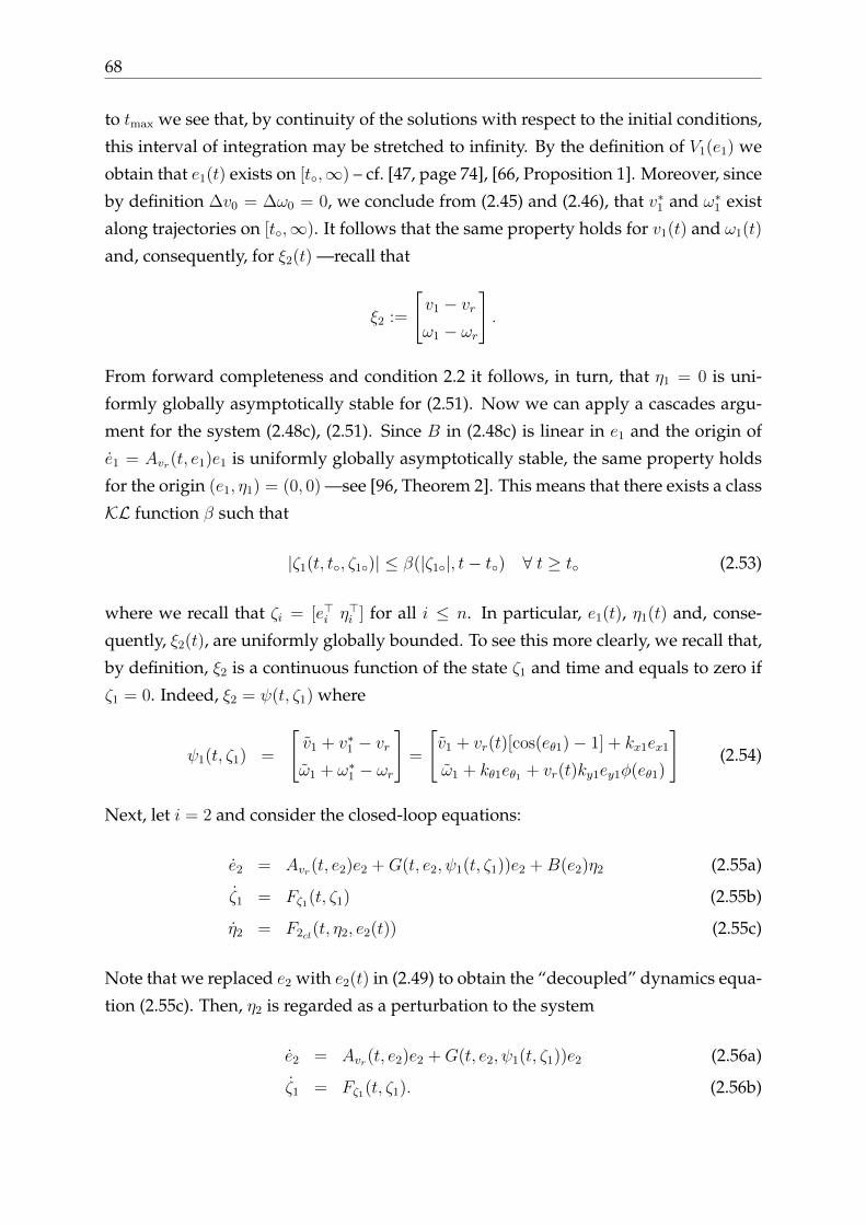
68
to tmax we see that, by continuity of the solutions with respect to the initial conditions,
this interval of integration may be stretched to infinity. By the definition of V1(e1) we
obtain that e1(t) exists on [t,∞) – cf. [47, page 74], [66, Proposition 1]. Moreover, since
by definition ∆v0 = ∆ω0 = 0, we conclude from (2.45) and (2.46), that v∗1 and ω∗1 exist
along trajectories on [t,∞). It follows that the same property holds for v1(t) and ω1(t)
and, consequently, for ξ2(t) —recall that
ξ2 :=
[v1 − vrω1 − ωr
].
From forward completeness and condition 2.2 it follows, in turn, that η1 = 0 is uni-
formly globally asymptotically stable for (2.51). Now we can apply a cascades argu-
ment for the system (2.48c), (2.51). Since B in (2.48c) is linear in e1 and the origin of
e1 = Avr(t, e1)e1 is uniformly globally asymptotically stable, the same property holds
for the origin (e1, η1) = (0, 0) —see [96, Theorem 2]. This means that there exists a class
KL function β such that
|ζ1(t, t, ζ1)| ≤ β(|ζ1|, t− t) ∀ t ≥ t (2.53)
where we recall that ζi = [e>i η>i ] for all i ≤ n. In particular, e1(t), η1(t) and, conse-
quently, ξ2(t), are uniformly globally bounded. To see this more clearly, we recall that,
by definition, ξ2 is a continuous function of the state ζ1 and time and equals to zero if
ζ1 = 0. Indeed, ξ2 = ψ(t, ζ1) where
ψ1(t, ζ1) =
[v1 + v∗1 − vrω1 + ω∗1 − ωr
]=
[v1 + vr(t)[cos(eθ1)− 1] + kx1ex1
ω1 + kθ1eθ1 + vr(t)ky1ey1φ(eθ1)
](2.54)
Next, let i = 2 and consider the closed-loop equations:
e2 = Avr(t, e2)e2 +G(t, e2, ψ1(t, ζ1))e2 +B(e2)η2 (2.55a)
ζ1 = Fζ1(t, ζ1) (2.55b)
η2 = F2cl(t, η2, e2(t)) (2.55c)
Note that we replaced e2 with e2(t) in (2.49) to obtain the “decoupled” dynamics equa-
tion (2.55c). Then, η2 is regarded as a perturbation to the system
e2 = Avr(t, e2)e2 +G(t, e2, ψ1(t, ζ1))e2 (2.56a)
ζ1 = Fζ1(t, ζ1). (2.56b)

Chapter 2 69
which, in turn, is also in cascaded form. Now, in view of the structure of G, we have
∂V1
∂eiG(t, ei, ξi)ei = 0, ∀ i ≤ n (2.57)
hence, the total derivative of V1 along the trajectories of (2.55a) yields
V1(e2(t)) ≤ c√V1(e2(t)) |η2(t)|[t0,tmax] ≤ c′V1(e2(t)) + d
with an appropriate redefinition of c and c′ –cf. Ineq. (2.52). Completeness of e2(t), and
therefore of η2(t), follows using similar arguments as for the case when i = 1. Conse-
quently, by Assumption 2.2, the origin of (2.55c) is uniformly globally asymptotically
stable.
To analyze the stability of the origin for (2.55) we invoke again [96, Theorem 2]. To
that end, we only need to establish uniform global asymptotic stability for the system
(2.56) (since B is linear and the origin of (2.55c) is uniformly globally asymptotically
stable). For this, we invoke [97, Theorem 4] as follows: first, we remark that the re-
spective origins of e2 = Avr(t, e2)e2 and (2.56b) are uniformly globally asymptotically
stable. Second, note that condition A4 in [97, Theorem 4] is not needed here since
we already established uniform forward completeness. Finally, [97, Ineq. (24)] holds
trivially with V = V1, in view of (2.57). We conclude that (e2, ζ1, η2) = (0, 0, 0) is a
uniformly globally asymptotically stable equilibrium of (2.55).
For i = 3 the closed-loop dynamics is
e3 = Avr(t, e3)e3 +G(t, e3, ψ2(t, ζ12)e3 +B(e3)η3 (2.58a)
ζ12 =: Fζ12(t, ζ12) (2.58b)
η3 = F3cl(t, η3, e3(t)) (2.58c)
where ζ12 := [ζ>1 ζ>2 ]>, ζ2 := [e>2 η>2 ], and
ψ2(t, ζ12) :=
[v2 + [ξ21 + vr(t)][cos(eθ1) + kx1ex1 − vrω2 + ξ22 + kθ1eθ1 + vr(t)ky1ey1φ(eθ1)
]
which corresponds to ξ3 —cf. (2.54). The previous arguments, as for the case i = 2,
apply now to (2.58) so the result follows by induction.
Remark 2.3. An example of torque controller for (2.2) that guarantees the integrability of the
vector [v1, ω1, ..., vN , ωN ] is presented in the first part, that is, when we assume that all the
system parameters are known, we end up with equation (2.14).
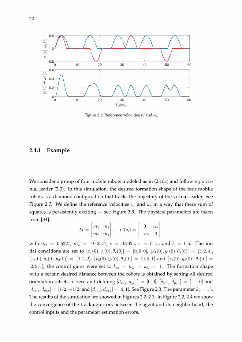
70
t(sec)0 10 20 30 40 50 60
v2 r(t)+ω2 r(t)
0
0.2
0.4
0.6
0 10 20 30 40 50 60
vr(t),ωr(t)
-0.5
0
0.5
Figure 2.1: Reference velocities vr and ωr
2.4.1 Example
We consider a group of four mobile robots modeled as in (2.10a) and following a vir-
tual leader (2.3). In this simulation, the desired formation shape of the four mobile
robots is a diamond configuration that tracks the trajectory of the virtual leader. See
Figure 2.7. We define the reference velocities vr and ωr in a way that there sum of
squares is persistently exciting — see Figure 2.5. The physical parameters are taken
from [34]:
M =
[m1 m2
m2 m1
], C(qi) =
[0 cω
−cω 0
],
with m1 = 0.6227, m2 = −0.2577, c = 0.2025, r = 0.15, and b = 0.5. The ini-
tial conditions are set to [xr(0), yr(0), θr(0)] = [0, 0, 0], [x1(0), y1(0), θ1(0)] = [1, 2, 4],
[x2(0), y2(0), θ2(0)] = [0, 2, 2], [x3(0), y3(0), θ3(0)] = [0, 5, 1] and [x4(0), y4(0), θ4(0)] =
[2, 2, 1]; the control gains were set to kxi = kyi = kθi = 1. The formation shape
with a certain desired distance between the robots is obtained by setting all desired
orientation offsets to zero and defining [dxr,1 , dyr,1 ] = [0, 0], [dx1,2 , dy1,2 ] = [−1, 0] and
[dx2,3 , dy2,3 ] = [1/2,−1/2] and [dx3,4 , dy3,4 ] = [0, 1]. See Figure 2.3, The parameter kd = 15.
The results of the simulation are showed in Figures 2.2–2.3. In Figure 2.2, 2.4 we show
the convergence of the tracking errors between the agent and its neighborhood, the
control inputs and the parameter estimation errors.

Chapter 2 71
t(sec)
0 10 20 30 40 50 60
‖ei(t)‖ i
=1,4
0
1
2
3
4
5
Figure 2.2: Exponential convergence of the relative errors (in norm) for each pair leader-follower
(xi)i=1,4(m)-2 0 2 4 6 8 10
(yi)i=
1,4(m
)
0
2
4
6
8
10
Figure 2.3: Illustration of the path-tracking in formation
t(sec)0 10 20 30 40 50 60
τi(t)
i=1,4
-100
-50
0
50
Figure 2.4: Illustration of the torque inputs for each agent

72
2.5 Leader-follower robust stabilization control
According to the robust stabilization control goal described in Problem 2.4, it is assumed
that
limt→∞|vr(t)|+ |ωr(t)| = 0 (2.59)
hence, in particular, the persistency of excitation condition, crucial to solve tracking
control problem, is violated.
Remark 2.4. The latter restriction naturally excludes control methods based on conditions of
persistency of excitation in Section 2.4 or, even more restrictive, that the references are always
separated from zero –cf. [23, 26, 67].
As we saw in Section 2.4, our control strategy consists in designing virtual control
laws v∗ and ω∗ for the kinematics equations (2.5) and, then, using them as references
for the dynamics equation (2.2). Our contribution resides in the fact that our kinemat-
ics controller is robust with respect to any controller at the force dynamics level. That
is, we establish convergence of the tracking errors for any controller [u1, u2] guarantee-
ing that v → v∗ and ω → ω∗, that is, the errors v := v − v∗ and ω = ω − ω∗ verify
limt→∞|v(t)|+ |ω(t)| = 0. (2.60)
Consider the virtual control laws
v∗ = kxex + vr(t) cos eθ (2.61a)
ω∗ = ωr(t) + kθeθ + ky[e2y + e2
x
]p(t) (2.61b)
under the standing assumption that p is persistently exciting —see Definition A.6, that
is, let there exist µ > 0 and T > 0 such that∫ t+T
t
p(s)2ds ≥ µ ∀t ≥ 0. (2.62)
This type of controller is called δ-persistently exciting —see [64, 67, 119]. For in-
stance, the term φ(t, x) := [e2y + e2
x]p(t), that appears in (2.61b), satisfies Definition A.7
with x = [ex, ey]> and p being persistently exciting. The mechanism relies on the prop-
erties of φ(t, x) which, roughly speaking, is persistently exciting as long as the tracking
errors are away from the origin.
For the controller (2.61), we establish strong integral input-to-state stability with
respect to the reference trajectories vr and ωr, as well as the velocity tracking errors
v = v − v∗ and ω = ω − ω∗. In particular, the tracking errors converge to zero for any
Chapter 2 73
reference velocities satisfying (2.59) and any converging velocity errors, even slowly-
converging.
Proposition 2.5. Consider the system (2.5) with v = v + v∗, ω = ω + ω∗, and (2.61). Let
kx, kθ, and ky > 0 and let p and p be bounded and persistently exciting. Then, the closed-loop
system is strongly integral input-to-state stable with respect to η := [vr ωr v ω]>.
Proof. We start by writing the closed-loop system (2.5) with (2.61) in the form of a
perturbed system, i.e.,
e = A(t, e)e+B(e)η (2.63)
where e := [ex ey eθ]>, η is a vanishing perturbation (due to (2.59) and (2.60)), and
A(t, e) :=
−kx ψ(t, e) 0
−ψ(t, e) 0 0
−kyp(t)ex −kyp(t)ey −kθ
,
B(e) =
0 ey −1 ey
sin(eθ) −ex 0 −ex0 0 0 −1
ψ(t, e) := kθeθ + kyp(t)[e2y + e2
x
].
Then, we carry out the analysis of stability for (2.63) in the following three steps:
1. we construct a strict Lyapunov function for the nominal system e = A(t, e)e;
2. we use this Lyapunov function to establish the small input-to-state stability prop-
erty with respect to the input η —see Appendix A.3 for the characterization of
small input-to-state stability using Lyapunov functions;
3. we establish integral input-to-state-stability of (2.63) with respect to η —see Ap-
pendix A.4 for the characterization of small input-to-state stability using Lya-
punov functions.
Remark 2.5. Proving the last three items is equivalent, by definition, to establishing the strong
input-to-state stability of (2.63) with respect to η —see Appendix A.5.
Step 1. UGAS of the nominal system e = A(t, e)e.

74
Let φm and φM > 0 and consider the positive differentiable function φ : R≥0 →[φm, φM ] satisfying
φ = −kθφ+ kyp(t). (2.64)
Such function exists because p is bounded and persistently exciting [112]. Then, con-
sider the new error coordinate
ez = eθ + φ(t)[e2y + e2
x
],
which satisfies
ez = −kθez − 2φkxe2x. (2.65)
Then, in the new coordinates, the nominal system becomes
[ex
ey
]=
[−kx φ[e2
y + e2x]
−φ[e2y + e2
x] 0
][ex
ey
]+ ez
[0 kθ
−kθ 0
][ex
ey
](2.66a)
ez = −kθez − 2φkxe2x (2.66b)
Now, since p is persistently exciting and φ satisfies the equation
φ = −kθφ+ p (2.67)
we conclude that φ is also persistently exciting [41, Lemma 4.8.3]. Based on these
properties, Lemma 2.1, below, provides a strict differentiable Lyapunov function for
(2.66).
Lemma 2.1 (set-point stabilization). Consider the following nonlinear time-varying system
[ex
ey
]=
[−kx φ[e2
y + e2x]
−φ[e2y + e2
x] 0
][ex
ey
]+ ez
[0 kθ
−kθ 0
][ex
ey
](2.68a)
ez = −kθez − 2φkxe2x (2.68b)
let kθ, kx > 0, φ : R≥0 → R, φ be persistently exciting and let
max|φ|∞, |φ|∞, |φ|∞
≤ φ

Chapter 2 75
where
|φ|∞ := ess supt≥0|φ(t)|
Then, the system (2.68) admits the following strict Lyapunov function
V3(t, e) := γ1
(V1(e)
)V1(e) + V2(t, e) + γ2
(V1(e)
)e2z (2.69)
where V1(e) := e2x + e2
y.
V2(t, e) := γ3
(V1(e)
)V1(e) + Υφ(s)2(t)V1(e)3 − φ(t)V1(e)exey (2.70)
Υφ(s)2(t) := 1 + φ2T − 1
T
∫ t+T
t
∫ m
t
φ(s)2dsdm, (2.71)
and γi : R≥0 → R≥0 are positive polynomials of V1 defined as
γ1(V1) :=µ
16TkxV 2
1 +1
2φV1 +
4kxφ2
kθγ2(V1)V1 +
1
2, (2.72)
γ2(V1) :=8T φ2kθµ
V1 + 1 (2.73)
γ3(V1) :=φ
kx
[2φV 2
1 +1
4
[3kx + 1
]V1 +
T φ
µ
[k2x + 1
]]. (2.74)
and its derivative satisfies the inequality
V3(t, e) ≤ − µ
8Te6y − kθγ2(V1)e2
z − kxe2x −
µ
4TV 3
1 . (2.75)
The proof of Lemma 2.1 is presented in the Appendix B.6, the construction of V3 is
inspired by [72].
Step 2. Small ISS property.
We recall that a system x = f(t, x, η) is said to be ”small ISS” if it is input-to-state
stable for sufficiently small values of η. See the Appendix A.3 for precise definitions.
The proof of this property for the system (2.63) relies on the function V3 constructed
in Lemma 2.1 above; specifically on the order of growth in V1. For the purpose of
76
analysis we remark that V3 in (2.69) can be written as
V3(t, e) ≡ V3(t, e, V1) (2.76)
where
V3(t, e, V1) := ρ(t, V1)V1 − φ(t)V1exey + γ2(V1)e2z (2.77)
ρ(t, V1) := [γ1(V1) + γ3(V1)]V1 + Υφ(s)2(t)V 31 (2.78)
that is, ρ : R≥0 × R≥0 → R≥0 is a smooth function, uniformly bounded in t (since
|Υφ(s)2(t)| ≤ 1 + φ2T ) and ρ(t, ·) is a polynomial of degree 2 with strictly positive
coefficients. In particular, since Υφ(s)2(t) ≥ 1,
∂ρ
∂V1
≥ 0 ∀ (t, V1) ∈ R≥0.× R≥0
Now, by Lemma 2.1 the time-derivative of V3 along the nominal system (2.66) satisfies
(2.75) hence, the time-derivative of V3 along the trajectories of (2.63) satisfies
V3 ≤−µ
4TV 3
1 − kθγ2(V1)e2z − kxe2
x −µ
8Te6y +
∂V3
∂eB(e)η. (2.79)
Now, note that B(e)η = K1(η)e+K2(η, e) where
K1(η) :=
0 ωr + ω 0
−(ωr + ω) 0 0
0 0 0
, K2(η, e) =
−v
vr sin eθ
−ω
,so using the fact that
∂V1
∂eK1(η)e = 0,
we obtain
V3 ≤ −µ
4TV 3
1 − kθγ2(V1)e2z − kxe2
x −µ
8Te6y − φ[ωr + ω]V1
[e2y − e2
x
]+∂V3
∂eK2(η, e)
≤− µ
4TV 3
1 − kθγ2(V1)e2z + φ
[|ωr|+ |ω|
]V 2
1 +
∣∣∣∣∂V3
∂e
∣∣∣∣ |K2|
− kxe2x −
µ
8Te6y. (2.80)

Chapter 2 77
On the other hand, from (2.77) and (2.76) we obtain∣∣∣∣∂V3
∂e
∣∣∣∣ ≤ 2
[∂ρ
∂V1
V1 + ρ(t, V1) + φV1
] [|ey|+ |ex|
]+ 2
∂γ2
∂V1
[|ey|+ |ex|
]e2z
+ 4γ2(V1)φ |ez|[|ey|+ |ex|
]+ 2γ2(V1)|ez|. (2.81)
Next, let us introduce the positive polynomial of second degree
γ4(V1) :=∂ρ
∂V1
V1 + ρ(t, V1) + φV1,
and the positive constant —see (2.73)
α :=∂γ2
∂V1
,
so that, using them in (2.81) and observing that |K2| ≤ |η|, we obtain
V3 ≤−µ
4TV 3
1 − kθγ2(V1)e2z + 2φ|η|V 2
1 − kxe2x −
µ
8Te6y
+ 2γ4(V1)|η|[|ey|+ |ex|
]+ 2α|η|
[|ey|+ |ex|
]e2z
+ 4γ2(V1)φ|η||ez|[|ey|+ |ex|
]+ 2γ2(V1)|η||ez|. (2.82)
Then, using the inequality |ez|[|ey|+ |ex|
]≤ e2
z + V1/2 in (2.82) we obtain
V3 ≤−µ
4TV 3
1 − kxe2x −
µ
8Te6y −
[[kθ − 4φ|η|
]γ2(V1)− 2α|η|
[|ey|+ |ex|
]− |η|
]e2z
+ 2φ|η|V 21 + 2γ4(V1)|η|
[|ey|+ |ex|
]+ 2γ2(V1)φ|η|V1 + γ2(V1)2|η|
≤ −[ µ
4TV 3
1 − Φ1(ex, ey)|η|]−[kθ
2γ2(V1)− Φ2(ex, ey)|η|
]e2z
− kxe2x −
µ
8Te6y −
kθ2γ2(V1)e2
z (2.83)
where
Φ1 := 2φV 21 + 2γ4(V1)
[|ey|+ |ex|
]+ 2γ2(V1)φV1 + γ2(V1)2,
Φ2 := 4φγ2(V1) + 2α[|ey|+ |ex|
]+ 1.
Then, since |ey|+ |ex| ≤√
2V1, γ2(V1) = O(V1), and γ4(V1) = O(V 21 ) there exist positive

78
constants ai, with i ∈ [0, 4], of innocuous values1, such that
Φ1 ≤ [a2V2
1 + a1V1 + a0][1 + a4V1/2
1 ] (2.84)
Φ2 ≤ a1V1 + a4V1/2
1 + a0. (2.85)
Furthermore, since V 1/21 ≤ a0 + a1V1 for all a0 ≥ 1, a1 ≥ 1, and V1 ≥ 0,
Φ1 ≤ a3V3
1 + a2V2
1 + a1V1 + a0 (2.86)
Φ2 ≤ a1V1 + a0. (2.87)
Now, let R > 0 and assume that η satisfies the following bound
|η| ≤ RminV1(e)3 + e2
z, 1
(2.88)
which, in particular, implies that |η| ≤ R. We see that the factor of e2z in (2.83) is non-
positive for sufficiently small R. Now, in regards to the term involving Φ1 in (2.83),
note that in case that V1 ≥ 1, since |η| ≤ R, we have Φ1|η| ≤ c1RV3
1 , and Φ2|η| ≤ c2RV1
for some c1, c2 > 0. Otherwise, if V1 ≤ 1, then there exists c3, c4 > 0 such that Φ1,2 ≤ c3,4
and, in view of (2.88),
Φ1|η| ≤ c3R [V 31 + e2
z], Φ2|η| ≤ c4R [V1 + 1] (2.89)
We conclude that, for sufficiently small R, (2.83) and (2.88) imply that
V3(t, e) ≤ −kθ4e2z − kxe2
x −µ
8Te6y
so the system is small-input-to-state stable.
Step 3. The iISS property.
The proof of Proposition 2.5 is finalized by establishing integral input-to-state sta-
bility of the system (2.63) with respect to η. To that end, consider the proper positive-
definite Lyapunov function
W (t, e) = ln(1 + V3(t, e)
)(2.90)
1Conventionally, ai (for any integer i ≥ 0) denote positive coefficients of polynomials so, withoutloss of generality, we implicitly assume that they are redefined as needed, e.g., ai := aiaj + a2i − ai . . .
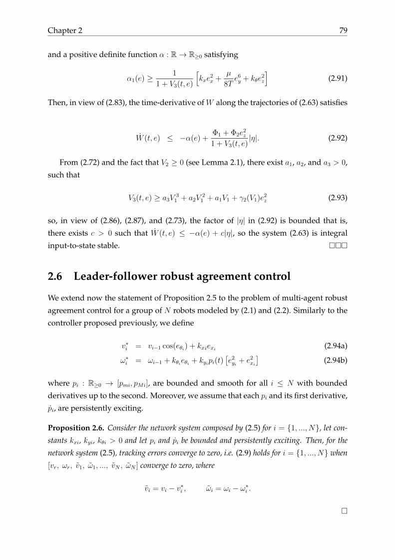
Chapter 2 79
and a positive definite function α : R→ R≥0 satisfying
α1(e) ≥ 1
1 + V3(t, e)
[kxe
2x +
µ
8Te6y + kθe
2z
](2.91)
Then, in view of (2.83), the time-derivative ofW along the trajectories of (2.63) satisfies
W (t, e) ≤ −α(e) +Φ1 + Φ2e
2z
1 + V3(t, e)|η|. (2.92)
From (2.72) and the fact that V2 ≥ 0 (see Lemma 2.1), there exist a1, a2, and a3 > 0,
such that
V3(t, e) ≥ a3V3
1 + a2V2
1 + a1V1 + γ2(V1)e2z (2.93)
so, in view of (2.86), (2.87), and (2.73), the factor of |η| in (2.92) is bounded that is,
there exists c > 0 such that W (t, e) ≤ −α(e) + c|η|, so the system (2.63) is integral
input-to-state stable.
2.6 Leader-follower robust agreement control
We extend now the statement of Proposition 2.5 to the problem of multi-agent robust
agreement control for a group of N robots modeled by (2.1) and (2.2). Similarly to the
controller proposed previously, we define
v∗i = vi−1 cos(eθi) + kxiexi (2.94a)
ω∗i = ωi−1 + kθieθi + kyipi(t)[e2yi
+ e2xi
](2.94b)
where pi : R≥0 → [pmi, pMi], are bounded and smooth for all i ≤ N with bounded
derivatives up to the second. Moreover, we assume that each pi and its first derivative,
pi, are persistently exciting.
Proposition 2.6. Consider the network system composed by (2.5) for i = 1, ..., N, let con-
stants kxi, kyi, kθi > 0 and let pi and pi be bounded and persistently exciting. Then, for the
network system (2.5), tracking errors converge to zero, i.e. (2.9) holds for i = 1, ..., N when
[vr, ωr, v1, ω1, ..., vN , ωN ] converge to zero, where
vi = vi − v∗i , ωi = ωi − ω∗i .

80
Proof. To compact the notation, let us define
V1i(ei) := e2xi
+ e2yi
(2.95)
ψi(t, ei) := kθieθi + kyipi(t)V1i
so that, replacing
vi = v∗i + vi, ωi = ωi + ω∗i , (2.96)
and (2.94) in (2.5) we obtain
exi = [ωi + ωi−1 + ψi]eyi − vi − kxiexi (2.97a)
eyi = −[ωi + ωi−1 + ψi]exi + vi−1 sin(eθi) (2.97b)
eθi = −ψi − ωi (2.97c)
which has exactly the same structure as (2.63). Indeed, the equations (2.97) may be
re-written in the compact form
ei = Ai(t, ei)ei +B(ei)ηi (2.98)
where ei := [eθi exi eyi ]>,
Ai(t, ei) :=
−kxi ψi(t, ei) 0
−ψi(t, ei) 0 0
−kyipi(t)exi −kyipi(t)eyi −kθi
ηi := [vi−1 ωi−1 vi ωi]
>.
As η in Proposition 2.5, which contains vr and ωr, ηi may also be regarded as a van-
ishing perturbation. To see more clearly, we develop some expressions for vi−1 and
ωi−1 to exhibit their dependence on vr and ωr. Using, recursively, (2.96) and (2.94a) we

Chapter 2 81
obtain
vi−1 = vi−2 cos(eθi−1) + kxi−1
exi−1+ vi−1
=[v2 + vi−3 cos(eθi−2
) + kxi−2exi−2
]cos(eθi−1
) + kxi−1exi−1
+ vi−1
= vi−1 + vi−2 cos(eθi−1) + vi−3 cos(eθi−2
) cos(eθi−1)
+ vi−4 cos(eθi−3) cos(eθi−2
) cos(eθi−1)
+ kxi−3exi−3
cos(eθi−2) cos(eθi−1
)
+ kxi−2exi−2
cos(eθi−1) + kxi−1
exi−1
...
=i−1∑j=1
[ [vj + kxjexj
] i−1∏k=j+1
cos(eθk)]
+ vr
i−1∏j=1
cos(eθj)
2while, from (2.94b),
ωi−1 = ωi−2 + kθi−1eθi−1
+ kyi−1pi−1(t)V1i−1 + ωi−1
= ωi−3 + kθi−2eθi−2
+ kyi−2pi−2(t)V1i−2
+ kθi−1eθi−1
+ kyi−1pi−1(t)V1i−1 + ωi−1 + ωi−2
...
= ωr(t) +i−1∑j=1
ψj.
So we see that for each robot indexed by i ≤ N , vi−1 and ωi−1 depend on the tracking
errors of all the followers, indexed up to i − 1, including the reference vehicle. For
i = 1, the system (2.98) corresponds to (2.63) hence, by Proposition 2.5, e1 → 0. For
i = 2, η2 := [v1, ω1, v1, ω1] where
v1 = v1 + kx1ex1 + vr cos(eθ1)
ω1 = ωr + kθ1eθ1 + ky1p1(t)V11
hence, η2 → 0 and, by Proposition 2.5 we obtain that e2 → 0. The statement follows by
induction.
Remark 2.6. An example of torque controller that guarantees convergence to zero of the vector
[v1, ω1, ..., vN , ωN ] is presented in Subsection 2.2.
2Conventionally,∏0
j=1 cos(·) = 1.
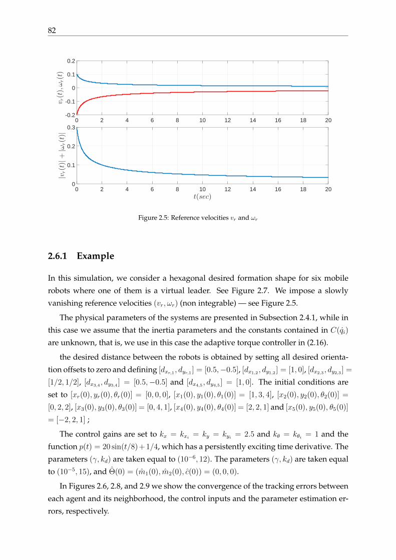
82
t(sec)0 2 4 6 8 10 12 14 16 18 20
|vr(t)|+|ω
r(t)|
0
0.1
0.2
0.30 2 4 6 8 10 12 14 16 18 20
vr(t),ωr(t)
-0.2
-0.1
0
0.1
0.2
Figure 2.5: Reference velocities vr and ωr
2.6.1 Example
In this simulation, we consider a hexagonal desired formation shape for six mobile
robots where one of them is a virtual leader. See Figure 2.7. We impose a slowly
vanishing reference velocities (vr, ωr) (non integrable) — see Figure 2.5.
The physical parameters of the systems are presented in Subsection 2.4.1, while in
this case we assume that the inertia parameters and the constants contained in C(qi)
are unknown, that is, we use in this case the adaptive torque controller in (2.16).
the desired distance between the robots is obtained by setting all desired orienta-
tion offsets to zero and defining [dxr,1 , dyr,1 ] = [0.5,−0.5], [dx1,2 , dy1,2 ] = [1, 0], [dx2,3 , dy2,3 ] =
[1/2, 1/2], [dx3,4 , dy3,4 ] = [0.5,−0.5] and [dx4,5 , dy4,5 ] = [1, 0]. The initial conditions are
set to [xr(0), yr(0), θr(0)] = [0, 0, 0], [x1(0), y1(0), θ1(0)] = [1, 3, 4], [x2(0), y2(0), θ2(0)] =
[0, 2, 2], [x3(0), y3(0), θ3(0)] = [0, 4, 1], [x4(0), y4(0), θ4(0)] = [2, 2, 1] and [x5(0), y5(0), θ5(0)]
= [−2, 2, 1] ;
The control gains are set to kx = kxi = ky = kyi = 2.5 and kθ = kθi = 1 and the
function p(t) = 20 sin(t/8)+1/4, which has a persistently exciting time derivative. The
parameters (γ, kd) are taken equal to (10−6, 12). The parameters (γ, kd) are taken equal
to (10−5, 15), and Θ(0) = (m1(0), m2(0), c(0)) = (0, 0, 0).
In Figures 2.6, 2.8, and 2.9 we show the convergence of the tracking errors between
each agent and its neighborhood, the control inputs and the parameter estimation er-
rors, respectively.

Chapter 2 83
t(sec)0 5 10 15 20 25 30
‖ei(t)‖i=
1,5
0
2
4
6
8
10
12
14
16
Figure 2.6: Exponential convergence of the relative errors (in norm) for each pair leader-follower
(xi)i=1,5(m)-2 -1.5 -1 -0.5 0 0.5 1 1.5 2 2.5
(yi)i=
1,5(m
)
-2
-1
0
1
2
3
4
leader
follower4
follower1
follower3
follower5
follower2
Figure 2.7: Illustration of the path-tracking in formation

84
t(sec)0 0.5 1 1.5 2 2.5 3 3.5 4 4.5 5
τi(t)
i=1,4
-1500
-1000
-500
0
500
1000
Figure 2.8: Illustration of the torque inputs for each agent
t(sec)0 0.2 0.4 0.6 0.8 1 1.2 1.4 1.6 1.8 2
∥ ∥ ∥Θ
i∥ ∥ ∥
i=1,5
0.64
0.65
0.66
0.67
0.68
0.69
0.7
Figure 2.9: Illustration of the estimation parameter errors for each agent
Chapter 2 85
2.7 Conclusion
In this chapter we considered the leader-follower control problem for single and mul-
tiple agent cases. We identified several control problems that impose distinct tech-
nical difficulties, depending on nature of the leader’s velocities. First, we presented
a formation-tracking controller for autonomous vehicles that ensures uniform global
asymptotic stability of the closed-loop system, under the assumption that either the
angular or the forward reference velocity is persistently exciting. Then, we consid-
ered the case where the leader’s velocities converge to zero and presented a simple
decentralized controller for leader-follower robust agreement problem. In both cases,
we assumed that each robot has only one leader and may have one or more followers.
Moreover, a strict Lyapunov function is provided for the kinematic error dynamics.
We decouple the problems at the velocity-kinematics and force-dynamics levels. Inter-
estingly enough, our results apply to a range of controllers at the dynamic level. Thus,
one can use a variety of control schemes for Lagrangian and Hamiltonian systems,
including adaptive and output feedback control designs.

86
Chapter 3
Leader-follower simultaneous
tracking-agreement control of
nonholonomic vehicles
In the previous chapter we presented several problem formulations for the forma-
tion control of nonholonomic vehicles, and emphasized how different scenarios of
the leader’s velocities influence both the control design and the stability properties
of the closed-loop system. Problem of unified controller that stabilizes the closed-
loop globally asymptotically for different scenarios of the leader’s velocities is a very
challenging problem. Indeed, to the best of our knowledge the simultaneous tracking-
stabilization problem for nonholonomic mobile robot has only been studied in [27, 52,
85, 119], where the goal is to design a unified velocity or torque controller for the fol-
lower robot in order to track the trajectories of the leader asymptotically under differ-
ent scenarios of the leader’s velocities. The possible scenarios include the case where
the leader describes a general time-varying path (tracking scenario), and stabilization
scenario where the leader converge to a set point (parking scenario) or, in a more gen-
eral case, where the leader’s velocities converge to zero robust stabilization scenario.
In [52] a saturated time-varying velocity controller is proposed to track the leader’s
trajectories under different scenarios of the leader’s velocities. In [85] a unified velocity
controller is provided to solve the problem under all possible configurations of the
leader’s velocities using the concept of transverse functions. In [27] and [119], a unified
torque controller is proposed in order to make the tracking error converging to the
origin under a tracking and a parking scenarios. In [119], a nice idea has been used
which consists of combining a tracking controller with stabilization controller via a
weighted sum, the weight function depends on the leader’s velocities and promotes
each controller depending on the current scenario.
87

88
For the multi-agent formation case, the unified controller proposed in [85] has been
extended to the leader-follower formation case in [118] under a general force con-
trolled model of the mobile robot, while assuming that the leader’s coordinates are
accessible to all the network. Providing a distributed solution to the leader-follower
simultaneous tracking-agreement control problem is an open question to the best of our
knowledge.
In this chapter, we propose to extend the idea of control design established in [119]
to a more general class of controllers, and thus to allow a more general scenarios of
the leader’s velocities as in [85]. Also our original proofs allow a straightforward
extension to the leader-follower simultaneous tracking-agreement case under spanning
communication graph topology. As in the previous chapter, our results are based on
the construction of strict Lyapunov functions for a nonlinear time-varying systems
[72], and robustness analysis tools such as the integral Input-to-state Stability [8, 9],
and the Strong integral Input-to-state Stability [17, 18].
3.1 A larger class of controllers
The simultaneous tracking-stabilization control problem has been addressed in [26]
and [119], where a unified control law is provided to guarantee the global attractivity
of the origin of (2.5) under each one of the following scenarios:
S1: Tracking scenario. It is assumed that there exists T and µ > 0 such that, for all
t ≥ t0: ∫ t+T
t
(|vr(τ)|2 + |ωr(τ)|2
)dτ > µ, ∀t ≥ t0. (3.1)
S2: Stabilization scenario. It is assumed that there exists β > 0 such that, for all
t ≥ t0: ∫ t
t0
(|vr(τ)|+ |ωr(τ)|)dτ < β, ∀t ≥ t0. (3.2)
Remark 3.1. Obviously, the two scenarios cannot appear simultaneously, but the goal is to
design a unified controller that guarantees the global attractivity of the origin of the closed-loop
system (2.5), independently of the actual scenario of the leader’s velocities.
In the first part of this chapter we consider simultaneous tracking and parking
problem and design a universal controller that achieves the trajectory tracking objec-
Chapter 3 89
tives
limt→∞
e(t) = 0 (3.3)
and,
limt→∞
(v, w) = (0, 0) (3.4)
under either of the two scenarios described above.
similar to Section 2.5, our contributions are the following:
• in the kinematic level, we propose control inputs v∗ and ω∗ that ensure uniform
global asymptotic stability of the origin of (2.5);
• on the dynamic level, for the velocity error kinematics in closed-loop, we estab-
lish integral input-to-state stability with respect to the error velocities [v, ω];
• for any control inputs u1 and u2 ensuring that v → 0 and ω → 0, we establish
global attractivity of the origin provided that the error velocities (v, ω) converge
sufficiently fast (they are square integrable).
The control laws that ensure the properties above are:
v∗ := vr(t) cos(eθ) + kxex, (3.5)
ω∗ := ωr + kθeθ + kyeyvrφ(eθ) + ρ(t)kyf(t, ex, ey) (3.6)
where φ is the so-called sync function defined by
φ(eθ) :=sin(eθ)
eθ,
the weight function ρ(t) is defined as
ρ(t) := exp
(−∫ t
0
[|vr(τ)|+ |ωr(τ)|
]dτ
), (3.7)
and f : R+ × R2 → R is a continuously differentiable function defined such that the
following technical assumptions hold.
Assumption 3.1. There exist non-decreasing function σ1 : R≥ → R≥0 and a constant σ2 > 0
such that
max
|∂f∂t|, | ∂f
∂ex|, | ∂f
∂ey|≤ σ1(|ex ey|) (3.8)
|f(t, ex, ey)| ≤ σ2|ex ey|. (3.9)
90
Assumption 3.2. Let f(t, ey) := f(t, 0, ey) then, ∂f∂t
(t, 0, ey) is uniform δ−persistently ex-
citing with respect to ey —see Definition A.7 or [65, Definition 3].
Roughly speaking, the purpose of the function f is to excite the ey–dynamics as
long as |ey| is separated from zero.
The controller (3.6) which achieves both the tracking and the stabilization control
goals, is a weighted sum of the tracking controller of [70],
ω∗tra := ωr + kθeθ + kyeyvrφ(eθ),
and the stabilization controller that generalizes the ones proposed in [71, 78, 119],
ω∗stab := ωr + kθeθ + kyf(t, ex, ey).
The weight function ρ(t) acts as a smoothly-switching supervisor promoting the appli-
cation of either ω∗tra or ω∗stab, depending on the task scenario S1 or S2. More precisely,
from (3.7) we see that ρ satisfies
ρ =−[|vr(t)|+ |ωr(t)|
]ρ (3.10)
and ρ → 0 exponentially fast if (3.1) holds. Hence, the tracking scenario S1 is pro-
moted. If, instead, (3.2) holds, the reference velocities converge and ρ(t) > exp (−β).
Hence, the action of the stabilization controller is favoured.
Remark 3.2. The idea of such merging of two controllers for the scenarios S1 and S2 was
initially introduced in [78]. The class of controllers satisfying Assumptions 3.1-3.2 covers
those in [119]; in particular, the function f is not necessarily globally bounded and may depend
only on ey. A more significant contribution with respect to the literature is that we establish
uniform global asymptotic stability for (2.5) in closed-loop with (v, ω) = (v∗, ω∗); this is in
contrast with [119] and [26] where it is proved that (3.3) holds. In addition, we establish
integral ISS of (2.5) with respect to [v, ω].
Proposition 3.1. Consider the system (2.5) with v = v + v∗, ω = ω + ω∗, and the virtual
inputs (3.5) and (3.6). Let kx, kθ, and ky > 0.
Assume that there exist ωr, ¯ωr, vr, ¯vr > 0 such that
|ωr|∞ ≤ ωr, |ωr|∞ ≤ ¯ωr, |vr|∞ ≤ vr, |vr|∞ ≤ ¯vr. (3.11)
Furthermore, let Assumptions 3.1-3.2 hold.
If either (3.1) or (3.2) is satisfied, then the closed-loop system resulting from (2.5), (2.6),
(3.5), and (3.6) has the following properties:
Chapter 3 91
(P1) if v = ω = 0, the origin e = 0 is uniformly globally asymptotically stable;
(P2) the closed-loop system is integral input-to-state stable with respect to η := [v ω]>;
(P3) if η → 0 and η ∈ L2, then (3.3) holds.
3.1.1 Proof of Proposition 3.1
For each scenario, S1 and S2 we establish uniform global asymptotic stability for the
closed-loop kinematics equation (2.5) restricted to η = 0. Then, we establish the iISS
with respect to η by showing that the closed-loop trajectories are bounded under the
condition that η is square integrable —cf. [8].
Under Scenario S1
The proof of Proposition 3.1 under condition (3.1) is constructive, in particular, we
provide a strict Lyapunov function for the closed loop system. To that end, we start by
observing that the error system (2.5), (2.6), (3.5) and (3.6) has the form
e =Avr(t, e)e+B1(t, e)ρ(t) +B2(e)η, (3.12)
where
Avr(t, e) :=
−kθ 0 −vr(t)kyφ(eθ)
0 −kx ω∗(t, e)
vr(t)φ(eθ) −ω∗(t, e) 0
,
B1(t, e) :=
−kyf(t, ex, ey)
kyf(t, ex, ey)ey
−kyf(t, ex, ey)ex
, B2(e) :=
0 −1
−1 ey
0 −ex
. (3.13)
Writing the closed-loop dynamics as in (3.12) is convenient to stress that the “nominal”
system e = Avr(t, e)e has a familiar structure encountered in model reference adaptive
control, see Section 1.3.1. Moreover, defining
V1(e) :=1
2
[e2x + e2
y +1
kye2θ
], (3.14)
we obtain, along the trajectories of e = Avr(t, e)e,
V1(e) ≤ −kxe2x − kθe2
θ.
92
This is a fundamental first step in the construction of a strict Lyapunov function for
the “perturbed” system (3.12).
To establish the proof in the case of scenario S1, we follow the steps 1− 3 below:
1) We build a strict Lyapunov function V (t, e) for the nominal system e = Avr(t, e)e.
This establishes P1.
2) We construct strict Lyapunov function W (t, e) for the perturbed system e =
Avr(t, e)e+B1(t, e)ρ.
3) We use W (t, e) to prove integral ISS of (3.12) with respect to η (i.e., P2) as well
as the boundedness of the trajectories under the assumption that η ∈ L2. This and the
assumption that η → 0 implies (3.3), i.e., P3.
Step 1. We establish UGAS for the nominal system
e = Avr(t, e)e (3.15)
via Lyapunov’s direct method. After Proposition 2.1, there exists a positive definite
radially unbounded function V : R≥0 × R3 → R≥0 defined as
V (t, e) := P[3](t, V1)V1(e)− ωr(t)exey+vr(t)P[1](t, V1)eθey, (3.16)
and such that
F[3](V1) ≤ V (t, e) ≤ S[3](V1), (3.17)
where V1(e) is defined in (3.14), F[3], S[3] : R≥0 → R≥0, and P[k] : R≥0 × R≥0 → R≥0 are
smooth polynomials in V1(e) with strictly positive and bounded coefficients of degree
3 and k respectively. It is shown in Proposition 2.1 that the total derivative of V (t, e)
along the trajectories of (3.15) satisfies
V (t, e) ≤ −µTV1(e)− kxe2
x − kθe2θ. (3.18)
Hence uniform global asymptotic stability of the null solution of (3.15) follows.
Step 2. Now we construct a strict Lyapunov function for the system
e =Avr(t, e)e+B1(t, e)ρ(t). (3.19)
To that end, we start by “reshaping” the function V (t, e) defined in (3.16) to obtain a
particular negative bound on its time-derivative. Let
Z(t, e) := Q[3](V1)V1(e) + V (t, e) (3.20)

Chapter 3 93
where Q[3](V1) is a third order polynomial with a strictly positive coefficients. Then, in
view of (3.18), the total derivative of Z along the trajectories of (3.15) satisfies
Z(t, e) ≤ −µTV1(e)−Q[3](V1)
[kxe
2x + kθe
2θ
]. (3.21)
Next, we recall that in view of (3.1) ρ is uniformly integrable hence, for any γ > 0,
there exists c > 0 such that
G(t) := exp
(−γ∫ t
0
ρ(s)ds
)≥ c > 0 ∀t ≥ 0. (3.22)
Thus, since Z(t, e) and V (t, e) are positive definite radially unbounded —see (3.17) and
(3.20), so is the function
W (t, e) := G(t)Z(t, e). (3.23)
Indeed, we have
exp
(−γ∫ ∞
0
ρ(s)ds
)Z(t, e) ≤ W (t, e) ≤ Z(t, e).
Now, the time-derivative of W along trajectories of (3.19) verifies
W (t, e) ≤ −Y (t, e) + G(t)Z(t, e) +G(t)∂(Q[3](V1)V1 + V
)∂e
B1(t, e)ρ(t)
Y (t, e) := G(t)[µTV1(e) +Q[3](V1)
[kxe
2x + kθe
2θ
]]. (3.24)
Note that, in view of (3.22), Y (t, e) is positive definite. We proceed to show that the
rest of the terms bounding W are negative semi-definite. To that end, we develop
(dropping the arguments of f(t, ex, ey) )
∂(Q[3](V1)V1 + V
)∂e
B1(t, e) =∂(Q[3](V1)V1 + V
)∂V1
∂V1
∂eB1(t, e)− ωrkyf(·)
[ex + e2
y
]− vrP[1](t, V1)kyf(·) [eθex + ey] (3.25)
and we decompose B1(t, e) into
B1(t, e) =
−kyf(·)
0
0
+
0 0 0
0 0 kyf(·)0 −kyf(·) 0
e.
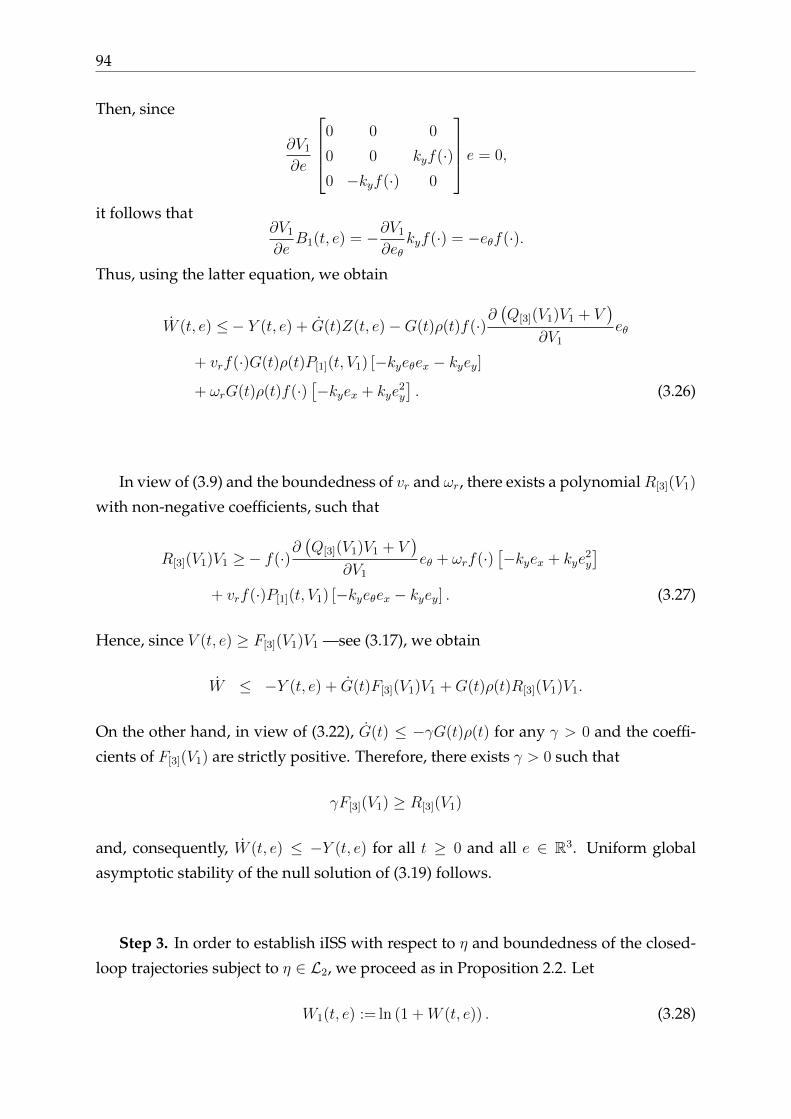
94
Then, since
∂V1
∂e
0 0 0
0 0 kyf(·)0 −kyf(·) 0
e = 0,
it follows that∂V1
∂eB1(t, e) = −∂V1
∂eθkyf(·) = −eθf(·).
Thus, using the latter equation, we obtain
W (t, e) ≤− Y (t, e) + G(t)Z(t, e)−G(t)ρ(t)f(·)∂(Q[3](V1)V1 + V
)∂V1
eθ
+ vrf(·)G(t)ρ(t)P[1](t, V1) [−kyeθex − kyey]
+ ωrG(t)ρ(t)f(·)[−kyex + kye
2y
]. (3.26)
In view of (3.9) and the boundedness of vr and ωr, there exists a polynomialR[3](V1)
with non-negative coefficients, such that
R[3](V1)V1 ≥− f(·)∂(Q[3](V1)V1 + V
)∂V1
eθ + ωrf(·)[−kyex + kye
2y
]+ vrf(·)P[1](t, V1) [−kyeθex − kyey] . (3.27)
Hence, since V (t, e) ≥ F[3](V1)V1 —see (3.17), we obtain
W ≤ −Y (t, e) + G(t)F[3](V1)V1 +G(t)ρ(t)R[3](V1)V1.
On the other hand, in view of (3.22), G(t) ≤ −γG(t)ρ(t) for any γ > 0 and the coeffi-
cients of F[3](V1) are strictly positive. Therefore, there exists γ > 0 such that
γF[3](V1) ≥ R[3](V1)
and, consequently, W (t, e) ≤ −Y (t, e) for all t ≥ 0 and all e ∈ R3. Uniform global
asymptotic stability of the null solution of (3.19) follows.
Step 3. In order to establish iISS with respect to η and boundedness of the closed-
loop trajectories subject to η ∈ L2, we proceed as in Proposition 2.2. Let
W1(t, e) := ln (1 +W (t, e)) . (3.28)

Chapter 3 95
The derivative of W1 along trajectories of (3.12) satisfies
W1 ≤ −Gm
µTV1(e) +Q[3]
[kxe
2x + kθe
2θ
]1 +W (t, e)
+
∣∣∂W∂eB2η
∣∣1 +W (t, e)
(3.29)
with Gm := exp(−γ∫∞
0ρ(t)dt
).
Next, we decompose B2(e)η introduced in (3.12) into
B2(e)η := B21(η) +B22(η)e
where
B21(η) :=
−ω−v0
, B22(η) :=
0 0 0
0 0 ω
0 −ω 0
.Then, using the fact that ∂V1
∂eB22(η)e = 0, defining
H(t, e) := Q[3] + P[3] +∂Q[3]
∂V1
V1 +∂P[3]
∂V1
V1 + vr |eθ| |ey|∂P[1]
∂V1
,
and
ξ =
[eθky
ex
], (3.30)
we obtain ∣∣∣∂W∂e
B2η∣∣∣ ≤ H(t, e)|ξ||η|+ ωr|ey||η|+ vrP[1]|ey||η|
+ ωrV1|η|+ vrP[1]|eθ||ex||η|
≤ H(t, e)[ 1
2ε|ξ|2 +
ε
2|η|2]
+ ωr
[ 1
2εV1 +
ε
2V1|η|2
]+ ωr
[ 1
2εV1 +
ε
2|η|2]
+ vr
[ 1
2εV1 +
ε
2P 2
[1]|η|2]
+ vrP[1]
[ 1
2εV1|eθ|2 +
ε
2|η|2]
≤[H(t, e) + vrP[1]k
2yV1
] 1
2ε|ξ|2 + [2ωr + vr]
1
2εV1
+ε
2|η|2
[H(t, e) + ωrV1 + ωr + vrP
2[1] + vrP[1]
].

96
Next, we choose ε > 0 such that
H(t, e) + vrP[1]k2yV1
ε|ξ|2 ≤ GmQ[3]
[kxe
2x + kθe
2θ
],
2ωr + vrε
≤ Gmµ
T.
Such ε > 0 exists because Q[3] is a third order polynomial of V1 with strictly positive
coefficients. So (3.29) becomes
W1 ≤ −Gm
2
µTV1(e) +Q[3]
[kxe
2x + kθe
2θ
]1 +W (t, e)
+D[3](V1)
1 +W (t, e)
ε
2|η|2 (3.31)
where D[3](V1) is a third order polynomial satisfying
H(t, e) + ωrV1 + ωr + vrP2[1] + vrP[1] ≤ D[3].
From the positivity of V , (3.17), and the definition of W , we have
GmQ[3](V1)V1 ≤ W1(t, e) ≤ S[3](V1)V1 (3.32)
hence,
W1 ≤ −Gm
2
µTV1(e) +Q[3](V1)
[kxe
2x + kθe
2θ
]1 + S[3](V1)
+D[3](V1)
1 +GmQ[3](V1)
ε
2|η|2 . (3.33)
This implies the existence of a positive constant c > 0 and a positive definite function
α(e) such that
W1 ≤− α(e) + c |η|2 . (3.34)
The result follows from Lemma A.4.
Under the scenario S2:
The proof of Proposition 3.1 under condition (3.2) relies on arguments for stability of
cascaded systems as well as on tools tailored for systems with persistency of excitation.
We start by rewriting the closed-loop equations in a convenient form for the anal-
ysis under the conditions of Scenario S2. To that end, to compact the notation, let us

Chapter 3 97
introduce
fρ(t, ex, ey) := ρ(t)f(t, ex, ey) (3.35)
Φ(t, eθ, ex, ey) = kθeθ + kyfρ(t, ex, ey) (3.36)
Then, the closed-loop equations become
e = fe(t, e) + g(t, e)η, η = [v ω]>, (3.37)
where
fe(t, e) :=
−kθeθ − kyfρ − kyvrφ(eθ)ey
−kxex + Φey +[ωr + kyvrφ(eθ)ey
]ey
−Φex −[ωr + kyvrφ(eθ)ey
]ex + vr sin eθ
,
g(t, e) :=
0 −1
−1 ey
0 −ex
.Following the proof-lines of [97, Lemma 1] for cascaded systems, we establish the
following for the system (3.37):
Claim 1. The solutions are uniformly globally bounded subject to η ∈ L2,
Claim 2. The origin of e = fe(t, e) is uniformly globally asymptotically stable (i.e., P1).
After [8] the last two claims together imply integral ISS with respect to η (i.e., P2).
Moreover, Claim 1 implies the convergence of the closed-loop trajectories to the origin
provided that the input η tends to zero and is square integrable (i.e., P3).
Proof of Claim 1. Let
W (e) := ln(1 + V1(e)), V1(e) :=1
2
[e2x + e2
y
]. (3.38)
The total derivative of V1 along the trajectories of (3.37) yields
V1(e) ≤ −kxe2x + |ex||v|+ |vr|| sin(eθ)||ey| (3.39)
hence,
W (e) ≤ 1
1 + V1
[− kx
2e2x + |vr||ey|+
v2
2kx
](3.40)
≤ |ey|1 + V1
|vr|+1
2kx[1 + V1]v2. (3.41)

98
Integrating on both sides of (3.41) along the trajectories, from t0 to t, and invoking
the integrability of vr and the square integrability of η we see that W (e(t)) is bounded
for all t ≥ t0. Boundedness of ex(t) and ey(t) follows since W is positive definite and
radially unbounded in (ex, ey).
Remark 3.3. For further development, we also emphasize that proceeding as above from In-
equality (3.40) we conclude that ex ∈ L2, uniformly in the initial conditions.
Next, we observe that the eθ–equation in (3.37) corresponds to an exponentially
stable system with bounded input u(t) = −kyvr(t)φ(eθ(t))ey(t) − kyfρ(t, ex(t), ey(t)) −ω(t) hence, we also have eθ ∈ L∞.
Proof of Claim 2.
Let η = 0 and, for further development, let us split the drift of the nominal system
e = fe(t, e) into the output injection form:
fe(t, e) = F (t, e) +K(t, e) (3.42)
where
K(t, e) :=
−kyvrφ(eθ)ey[
ωr + kyvrφ(eθ)ey]ey
−[ωr + kyvrφ(eθ)ey
]ex + vr sin eθ
(3.43)
and
F (t, e) :=
−kθeθ − kyfρ−kxex + Φey
−Φex
.To establish UGAS for the origin of e = fe(t, e) we invoke the output-injection
lemma–see Appendix A.6. According to the latter, UGAS follows if:
a) there exist: an “output” y, non decreasing functions k1, k2, and β: R≥0 → R≥0, a class
K∞ function k, and a positive definite function γ such that, for all t ≥ 0 and all e ∈ R3,
|K(t, e)| ≤ k1(|e|)k(|y|) (3.44)
|y(t, e)| ≤ k2(|e|) (3.45)∫ ∞
γ(|y(t)|
)dt ≤ β(|e(0)|); (3.46)
b) the origin of e = fe(t, e) is uniformly globally stable;
c) the origin of e = F (t, e) is UGAS.
Condition a. Using (3.43), a direct computation shows that there exists c > 0 such
that
|K(t, e)| ≤ c(|e|2 + |e|
)| [vr ωr] |, (3.47)

Chapter 3 99
so (3.44) holds with k1(s) := c(s2 + s), k(s) := s, and y := [vr ωr]. Moreover, (3.45) and
(3.46) hold with γ(s) = s, since [vr ωr] ∈ L1, for a constant functions β and k2 which,
moreover, are independent of the initial state.
Condition b. Uniform global stability is tantamount to uniform stability and uni-
form global boundedness of the solutions —see [36]. The latter was established al-
ready for the closed-loop system under the action of the “perturbation” η hence, it
holds all the more in this case, where η = 0.
In order to establish uniform stability, we use Lyapunov’s direct method. Let R > 0 be
arbitrary but fixed.
We claim that, for the system e = F (t, e), there exists a Lyapunov function candidate
V : R≥0 × R3 → R≥0 and positive constants α1, α2, and α3 such that
α1 |e|2 ≤ V (t, e) ≤ α2 |e|2 ∀t ≥ 0, e ∈ R3 (3.48)∣∣∣∂V (t,e)∂e
∣∣∣ ≤ α3 |e| ∀t ≥ 0, e ∈ R3 (3.49)∂V∂t
+ ∂V∂eF (t, e) ≤ 0 ∀t ≥ 0, e ∈ BR. (3.50)
Furthermore, from (3.47) it follows that, for all t ≥ 0 and all e ∈ BR,
|K(t, e)| ≤ c(R + 1)[|vr|+ |ωr|
]|e|.
Then, evaluating the time derivative of V along the trajectories of (3.42), we obtain, for
all e ∈ BR,
V (t, e) ≤ ∂V (t, e)
∂eK(t, e) ≤ α3c(R + 1)
[|vr|+ |ωr|
]|e|2
≤ α3c(R + 1)
α1
[|vr|+ |ωr|
]V (t, e). (3.51)
Defining v(t) := V (t, e(t)) and invoking the comparison lemma, we conclude, for all
e ∈ BR, that
v(t) ≤ exp
(cα3(R + 1)
α1
∫ ∞t
(|vr(s)|+ |ωr(s)|) ds)v(t)
and, in view of the integrability condition (3.2), we obtain
|e(t)|2 ≤ α2
α1
exp
(α3c(R + 1)
α1
β
)|e(t)|2
Thus, uniform stability of (3.42) follows.
It is left to construct a Lyapunov function candidate V for the system e = F (t, e), that
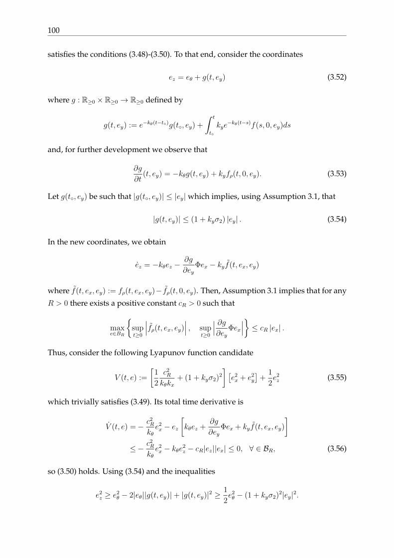
100
satisfies the conditions (3.48)-(3.50). To that end, consider the coordinates
ez = eθ + g(t, ey) (3.52)
where g : R≥0 × R≥0 → R≥0 defined by
g(t, ey) := e−kθ(t−t)g(t, ey) +
∫ t
t
kye−kθ(t−s)f(s, 0, ey)ds
and, for further development we observe that
∂g
∂t(t, ey) = −kθg(t, ey) + kyfρ(t, 0, ey). (3.53)
Let g(t, ey) be such that |g(t, ey)| ≤ |ey|which implies, using Assumption 3.1, that
|g(t, ey)| ≤ (1 + kyσ2) |ey| . (3.54)
In the new coordinates, we obtain
ez = −kθez −∂g
∂eyΦex − kyf(t, ex, ey)
where f(t, ex, ey) := fρ(t, ex, ey)− fρ(t, 0, ey). Then, Assumption 3.1 implies that for any
R > 0 there exists a positive constant cR > 0 such that
maxe∈BR
supt≥0
∣∣∣fρ(t, ex, ey)∣∣∣ , supt≥0
∣∣∣ ∂g∂ey
Φex
∣∣∣ ≤ cR |ex| .
Thus, consider the following Lyapunov function candidate
V (t, e) :=
[1
2
c2R
kθkx+ (1 + kyσ2)2
] [e2x + e2
y
]+
1
2e2z (3.55)
which trivially satisfies (3.49). Its total time derivative is
V (t, e) =− c2R
kθe2x − ez
[kθez +
∂g
∂eyΦex + kyf(t, ex, ey)
]≤− c2
R
kθe2x − kθe2
z − cR|ez||ex| ≤ 0, ∀ ∈ BR, (3.56)
so (3.50) holds. Using (3.54) and the inequalities
e2z ≥ e2
θ − 2|eθ||g(t, ey)|+ |g(t, ey)|2 ≥1
2e2θ − (1 + kyσ2)2|ey|2.
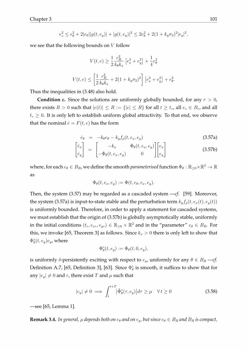
Chapter 3 101
e2z ≤ e2
θ + 2|eθ||g(t, ey)|+ |g(t, ey)|2 ≤ 2e2θ + 2(1 + kyσ2)2|ey|2,
we see that the following bounds on V follow
V (t, e) ≥ 1
2
c2R
kθkx
[e2x + e2
y
]+
1
4e2θ
V (t, e) ≤[
1
2
c2R
kθkx+ 2(1 + kyσ2)2
] [e2x + e2
y
]+ e2
θ.
Thus the inequalities in (3.48) also hold.
Condition c. Since the solutions are uniformly globally bounded, for any r > 0,
there exists R > 0 such that |e(t)| ≤ R := |e| ≤ R for all t ≥ t, all e ∈ Br, and all
t ≥ 0. It is only left to establish uniform global attractivity. To that end, we observe
that the nominal e = F (t, e) has the form
eθ = −kθeθ − kyfρ(t, ex, ey) (3.57a)[ex
ey
]=
[−kx Φθ(t, ex, ey)
−Φθ(t, ex, ey) 0
][ex
ey
](3.57b)
where, for each eθ ∈ BR, we define the smooth parameterised function Φθ : R≥0×R2 → Ras
Φθ(t, ex, ey) := Φ(t, eθ, ex, ey).
Then, the system (3.57) may be regarded as a cascaded system —cf. [59]. Moreover,
the system (3.57a) is input-to-state stable and the perturbation term kyfρ(t, ex(t), ey(t))
is uniformly bounded. Therefore, in order to apply a statement for cascaded systems,
we must establish that the origin of (3.57b) is globally asymptotically stable, uniformly
in the initial conditions (t, ex, ey) ∈ R≥0 × R2 and in the “parameter” eθ ∈ BR. For
this, we invoke [65, Theorem 3] as follows. Since kx > 0 there is only left to show that
Φθ(t, ey)ey, where
Φθ(t, ey) := Φθ(t, 0, ey),
is uniformly δ-persistently exciting with respect to ey, uniformly for any θ ∈ BR —cf.
Definition A.7, [65, Definition 3], [63]. Since Φθ is smooth, it suffices to show that for
any |ey| 6= 0 and r, there exist T and µ such that
|ey| 6= 0 =⇒∫ t+T
t
∣∣Φθ(τ, ey)∣∣dτ ≥ µ ∀ t ≥ 0 (3.58)
—see [65, Lemma 1].
Remark 3.4. In general, µ depends both on eθ and on ey, but since eθ ∈ BR andBR is compact,

102
by continuity, one can always choose the smallest qualifying µ, for each fixed ey. Therefore, as
in [65], µ may be chosen as a class K function dependent of |ey| only.
Now, we show that (3.58) holds under Assumption 3.2. To that end, we remark
that
Φθ(t, ey) = kθeθ + kyρ(t)f(t, ey)
–cf. Eq. (3.36), satisfies
Φθ = −kθΦ + kyρf + kyρ∂f∂t− kyρ
∂f∂ey
Φex
where we used eθ = −Φ and ey = Φex. Therefore, defining
KΦ(t, e) := kθ[Φθ − Φ]− kyρ
∂f∂ey
Φex
we obtain
Φθ = −kθΦθ − kyρ∂f∂t
+ kyρf +KΦ(t, e).
The latter equation corresponds to that of a linear filter with state Φθ and input
Ψ(t, ey) := −kyρ(t)∂f∂t
(t, ey) + kyρ(t)f(t, ey) +KΦ(t, e(t))
therefore, after [66, Property 4], Φθ is uniformly δ-PE with respect to ey, if so is Ψ. Now,
from Assumption 3.2 and uniform global boundedness of the solutions, for any r there
exists c > 0 such that
∣∣kyρ(t)f(t, ey(t)) +KΦ(t, e(t))∣∣ ≤ c(r)
[|ex(t)|+ |ρ(t)|
]Therefore, uniform δ-PE with respect to ey of Ψ follows from Assumption A2 and the
fact that ρ and ex are uniformly square integrable. That ρ ∈ L2, with a bound uniform
in the initial times, follows from (3.10) because vr, ωr, and ρ are bounded and |vr|+ |ωr|is uniformly integrable. That ex is uniformly L2 follows from (3.40) —see Remark 3.3.
This concludes the proof of UGAS for the nominal system e = fe(t, e) hence, Claim 2.
is proved.
This completes the proof of Proposition 3.1.
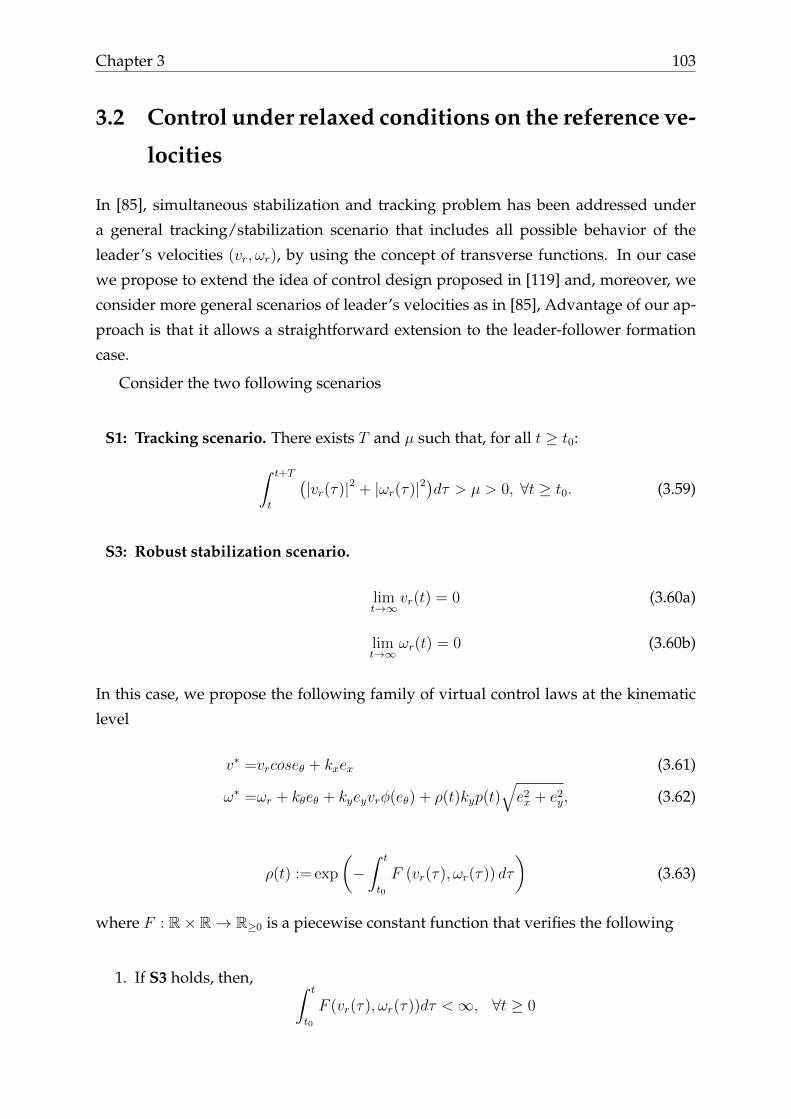
Chapter 3 103
3.2 Control under relaxed conditions on the reference ve-
locities
In [85], simultaneous stabilization and tracking problem has been addressed under
a general tracking/stabilization scenario that includes all possible behavior of the
leader’s velocities (vr, ωr), by using the concept of transverse functions. In our case
we propose to extend the idea of control design proposed in [119] and, moreover, we
consider more general scenarios of leader’s velocities as in [85], Advantage of our ap-
proach is that it allows a straightforward extension to the leader-follower formation
case.
Consider the two following scenarios
S1: Tracking scenario. There exists T and µ such that, for all t ≥ t0:∫ t+T
t
(|vr(τ)|2 + |ωr(τ)|2
)dτ > µ > 0, ∀t ≥ t0. (3.59)
S3: Robust stabilization scenario.
limt→∞
vr(t) = 0 (3.60a)
limt→∞
ωr(t) = 0 (3.60b)
In this case, we propose the following family of virtual control laws at the kinematic
level
v∗ =vrcoseθ + kxex (3.61)
ω∗ =ωr + kθeθ + kyeyvrφ(eθ) + ρ(t)kyp(t)√e2x + e2
y, (3.62)
ρ(t) := exp
(−∫ t
t0
F (vr(τ), ωr(τ)) dτ
)(3.63)
where F : R× R→ R≥0 is a piecewise constant function that verifies the following
1. If S3 holds, then, ∫ t
t0
F (vr(τ), ωr(τ))dτ <∞, ∀t ≥ 0

104
2. If S1 holds, then, there exists T1 and µ1 such that∫ t+T1
t
F (vr(s), ωr(s))2 ds ≥ µ1, ∀t ≥ 0.
Remark 3.5. The definition of ρ in (3.63) covers that in (3.7) employed in the previous section.
The following lemma establishes the existence of F by providing a candidate that sat-
isfies the last two items
Lemma 3.1. Let α(t) :=√v2r(t) + ω2
r(t), where vr(t) and ωr(t) are two scalar continuous
functions. Assume that there exists α > 0 such that |α(t)|∞ ≤ α. Then, the functional
F (vr, ωr) := K(α) :=
α if α ∈ (0, µ
2T α]
0 Otherwise(3.64)
satisfies the following:
1. K(α(t)) is PE, if α(t) is PE.
2. K(α(t)) is integrable, if limt→∞ α(t) = 0 .
Proof. The proof of the second item is trivial, because K(α) is null after finite time Tf ,
and ∫ t
0
K(α(s))ds ≤∫ Tf
0
K(α(s))ds, ∀t ≥ 0.
To prove the first item, we use [63, Lemma 2] which states that, if α(t) is PE(∫ t+T
tα(τ)dτ ≥ µ
).
Then for every t ≥ 0 there exists a non null measure set
It := τ ∈ [t, t+ T ] : |α(τ)| ≥ a := µ/(2T α) ,
and
meas(It) ≥ b := Tµ/(2T α2 − µ).
Using this lemma we obtain∫ t+T
t
K2(α(s))ds ≥∫It
K2(α(s))ds ≥∫It
a2ds ≥ a2b > 0.
Hence is K(α(s)) PE.
Proposition 3.2. Consider the system (2.5) with v = v + v∗, ω = ω + ω∗, and the virtual
inputs (3.61) and (3.62). Let kx, kθ, and ky > 0; let p and p be bounded and persistently
exciting, and assume that there exist ωr, ¯ωr, vr, ¯vr > 0 such that (3.11) holds. Then,

Chapter 3 105
1) Under the condition of scenario S1, the closed-loop system is integral input-to-state sta-
ble with respect to η1 := [v ω]>. Moreover, if η is a converging square integrable func-
tion, then the closed-loop trajectories converge to the origin.
2) Under the condition of scenario S3, the closed-loop system is strongly integral input-to-
state stable with respect to η2 := [vr ωr v ω]>.
3.2.1 Proof of Proposition 3.2
Under the scenario S1:
We decompose the closed-loop system as follows
e =Avr(t, e)e+B1(t, e)ρ(t) +B2(e)η, (3.65)
where
Avr(t, e) :=
−kθ 0 −vr(t)kyφ(eθ)
0 −kx ω∗(t, e)
vr(t)φ(eθ) −ω∗(t, e) 0
, B1(t, e) :=
−kyp(t)
√e2y + e2
x
kyp(t)√e2y + e2
xey
−kyp(t)√e2y + e2
xex
,
B2(e) :=
0 −1
−1 ey
0 −ex
. (3.66)
The proof under S1, follows exactly the same steps as in Proposition 3.1.
Under the scenario S3:
We start by rewriting the closed-loop system as
e = A(t, e)e+B(e)η2 (3.67)

106
where
A(t, e) :=
−kθ −kyp1(t)
√e2x+e2yex
−kyp1(t)
√e2x+e2yey
0 −kx ψ(t, e)
0 −ψ(t, e) 0
,ψ(t, e) := kθeθ + kyp1(t)
√e2y + e2
x.
B(e) =
−kyeyφ(eθ) 0 0 −1
kye2yφ(eθ) ey −1 ey
sin(eθ)− kyexeyφ(eθ) −ex 0 −ex
To establish the strong iISS property of the closed-loop system with respect to η2, we
follow the same proof steps as for Proposition 2.5. That is,
Step 1. we construct strict Lyapunov function for the closed-loop system when
η2 = 0;
Step 2. we establish the small ISS property of the closed-loop with respect to η2;
Step 3. we establish the integral ISS property of the closed-loop with respect to η2.
Remark 3.6. To simplify the computations, we introduce
p1(t) := ρ(t)p(t), (3.68)
where ρ(t) is given in (3.63). It is important to notice that under S3, p1(t) has the same
properties as p(t). That is, functions p1 and p1 are bounded and, since ρ(t) converges to zero
as t→∞, then p1(= ρp+ pρ) is PE if p is so –see Lemma A.9 in the Appendix.
Step 1. UGAS of the nominal system e = A(t, e)e.
Let ψm, ψM and ψM ≥ ψm > 0 and consider a positive differentiable function ψ :
R≥0 → [ψm, ψM ] satisfying
ψ = −kθψ + kyp1(t). (3.69)
Such a function exists because p1 is bounded and persistently exciting [112]. Then,
consider the new error coordinate
ez = eθ + ψ(t)√e2y + e2
x,
which satisfies
ez = −kθez − ψkxe2x√
e2x + e2
y
. (3.70)

Chapter 3 107
In the new coordinates, the nominal system becomes[ex
ey
]=
[−kx ψ
√e2y + e2
x
−ψ√e2y + e2
x 0
][ex
ey
]+ ez
[0 kθ
−kθ 0
][ex
ey
](3.71a)
ez = −kθez − ψkxex√e2x + e2
y
ex (3.71b)
Remark 3.7. Note that, by replacing ez with the trajectories ez(t) the system (3.71) covers a
cascaded form —see [59, 97]. Moreover, it is easy to show that ex and ey are bounded.
Now, since p1 is persistently exciting (see Remark 3.6) and ψ satisfies the equation
ψ = −kθψ + p1 (3.72)
we can conclude that function ψ is also persistently exciting [41, Lemma 4.8.3]. Based
on these properties, Lemma 3.2 below provides a strict differentiable Lyapunov func-
tion for the system (3.71).
Lemma 3.2 (set-point stabilization). Consider the following nonlinear time-varying system
[ex
ey
]=
[−kx ψ
√e2y + e2
x
−ψ√e2y + e2
x 0
][ex
ey
]+ ez
[0 kθ
−kθ 0
][ex
ey
](3.73a)
ez = −kθez − ψkxe2x√
e2x + e2
y
(3.73b)
let kθ, kx > 0, ψ : R≥0 → R and ψ be persistently exciting and let
max|ψ|∞, |ψ|∞, |ψ|∞
≤ ψ
where
|ψ|∞ := ess supt≥0|ψ(t)|
Then, the system (3.73) admits the following strict Lyapunov function:
V2(t, e) := P1(V1)V1(e) + Υψ(s)2(t)V1(e)2 − ψ(t)√V1exey +Q1(V1)e2
z (3.74)
where V1(e) := e2x + e2
y,
Υψ(s)2(t) := 1 + ψ2T − 1
T
∫ t+T
t
∫ m
t
ψ(s)2dsdm (3.75)
— cf (1.4), P1 and Q1 : R≥0 → R≥0 are first order polynomials of V1 with positive coefficients
108
defined as
P1(V1) :=1
kxψ2V1 + ψ
V1
4+
kx4kθ
ψ2Q1(V1) + ψ2T (kx + kθ)
4µV1 + 1, (3.76)
Q1(V1) :=T (kx + kθ)
µψ2V1 + 1. (3.77)
with
V2(t, e) ≤ −1
2kθQ1(V1)e2
z −µ
2TV 2
1 . (3.78)
The proof of Lemma 3.2 is presented in the Appendix B.7. Step 2. Small ISS prop-
erty.
Similarly to the proof of Proposition 2.5 in the previous Chapter, the proof of the
small ISS property, for the closed-loop system (3.67) with respect to η2, relies on the
function V2 constructed in Lemma 3.2 above; specifically on its order of growth in V1.
For the purpose of analysis we recall that V2 in (3.74) satisfies
V2(t, e) ≥ P1(V1)V1 − ψ√V1exey +Q1(V1)e2
z, (3.79)
where P1(V1) and Q1(V1) are first order polynomials with respect to V1 with positive
coefficients and time-derivative of V2(t, e) along the nominal part verifies
V2(t, e) = − µ
2TV 2
1 − kθQ1(V1)
2e2z (3.80)
To establish the small ISS property of the closed-loop with respect to η, let us consider
the time-derivative of V2 along trajectories of (3.67)
V2(·) ≤− µ
2TV 2
1 − kθQ1(V1)
2e2z +
∂V2
∂eB(e)η (3.81)
After decomposing B(e)η as
B(e)η := B1(η, e)e+B2(η, e), (3.82)
with
B1 =
0 0 0
0 0 (ω + ωr + kyvreyφ(eθ))
0 − (ωr + ω + kyvreyφ(eθ)) 0
,

Chapter 3 109
and
B2 =
−ω − kyvreyφ(eθ)
v
vr sin eθ
.and using the fact that
∂V1
∂eB1e = 0. (3.83)
we obtain
V2(·) ≤− µ
2TV 2
1 − kθQ1(V1)
2e2z − 2ψ(ωr + ω)
√V1
[e2y − e2
x
]−
ψ√V1eyvr
[e2y − e2
x
]+∂V2
∂eB2
≤− µ
2TV 2
1 − kθQ1(V1)
2e2z + 2ψ |ωr + ω|
√V1V1
+ ψ√V1 |ey| |vr|V1 +
∂V2
∂eB2. (3.84)
Next, we upperbound the term ∂V2
∂eB2∣∣∣∣∂V2
∂eB2
∣∣∣∣ ≤(P1(V1) +∂P1
∂V1
V1 + 2ψ√V1
)|[ex, ey]| |[v, vr]|
+
(∂Q1
∂V1
e2z |[ex, ey]|+Q1(V1) |ψez|
)|[v, vr]|
+Q1(V1) |ez| |ey| |vr|+Q1(V1) |ez| |ω| (3.85)
to obtain the following bound on V2
V2(·) ≤− µ
2TV 2
1 − kθQ1(V1)
2e2z + 2ψ |ωr + ω|
√V1V1 + ψ
√V1 |ey| |vr|V1
+
(P1 +
∂P1
∂V1
V1 + 2ψ√V1
)√V1 |η|
+
(∂Q1
∂V1
e2z
√V1 +Q1(V1)ψ |ez|
)|η|
+Q1(V1) |ez| |ey| |vr|+Q1(V1) |ez| |ω| .

110
≤− µ
2TV 2
1 − kθQ1(V1)
2e2z + 4ψ |η|
√V1V1 + ψ |η|V 2
1
+
(P1 +
∂P1
∂V1
V1 + 2ψ√V1
)√V1 |η|
+
(∂Q1
∂V1
V1e2z +Q1(V1)ψ2 +Q1(V1)e2
z
)|η|
+Q1(V1)(e2z + V1) |η|+Q1(V1)(e2
z + 1) |η| .
≤− V 21
[ µ2T−(ψ +Q11
)|η|]
+ 2P11V1
√V1 |η|
+ 4ψ |η|√V1V1 + 2ψ |η|V1 + P12
√V1 |η|
+Q1(V1)[ψ2 + 1
]|η|+Q12V1 |η| −
Q1(V1)
2e2z
[kθ2− 4 |η|
]. (3.86)
where Q11, Q12, P11, and P12 are positive constants, such that
Q1(V1) := Q11V1 +Q12, P1(V1) := P11V1 + P12.
So the small ISS property of (3.67) with respect to η follows by observing that the
system is ISS with respect to η for all η satisfying the bound
|η| < min
kθ8,
µ
2T(ψ +Q11
) ,Step 3. The iISS property.
The proof of Proposition 3.2 is finalized by establishing integral input-to-state sta-
bility of the system (3.67) with respect to η. To that end, we proceed similar to Propo-
sition 3.1 and we consider the proper positive-definite Lyapunov function
W2(t, e) = ln (1 + V2(t, e)) (3.87)
We can see that W2(t, e), is a proper Lyapunov function since so is V2. Moreover, the
total time-derivative of W2 along trajectories of the closed-loop system yields
W2 =V2
1 + V2
≤ −µ
2TV 2
1 + kθQ1(V1)
2e2z
1 + V2
+∂V2
∂eBη/(1 + V2) (3.88)
From (3.76) and (3.77), we conclude that there exists a first order polynomial g1(V1)

Chapter 3 111
with a strictly positive coefficients, such that
V2(t, e) ≥ g1(V1)(V1 + e2
z
)(3.89)
From this, it follows that there exists a class K function α such that:
α(|e|) ≤µ
2TV 2
1 + kθq1(V1)
2e2z
1 + V2(t, e). (3.90)
Then, using (3.82), (3.83) and the inequality (3.85), we can bound W2(t, e) as
W2 ≤− α(|e|) +2ψ |ωr + ω|
√V1V1
1 + g1(V1)V1
+ψ√V1 |ey| |vr|V1
1 + g1(V1)V1
+
(P1(V1) + ∂P1
∂V1V1 + 2ψ
√V1
)|[ex, ey]| |[v, vr]|
1 + g1(V1)V1
+
(∂Q1
∂V1e2z |[ex, ey]|+Q1(V1) |ψez|
)|[v, vr]|
1 + g1(V1) (e2z + V1)
+Q1(V1) |ez| |ey| |vr|+Q1(V1) |ez| |ω|
1 + g1(V1)(e2z + V1)
≤− α(|e|) +2ψ |ωr + ω|
√V1V1
1 + g1(V1)V1
+ψ |vr|V 2
1
1 + g1(V1)V1
+
(P1(V1)
√V1 + ∂P1
∂V1V1
√V1 + 2ψV1
)|η|
1 + g1(V1)V1
+
(∂Q1
∂V1e2z(V1 + 1) +Q1(V1) (ψ2e2
z + 1))|η|
1 + g1(V1) (e2z + V1)
+Q1(V1) (e2
z + V1) |vr|+Q1(V1) (e2z + 1) |ω|
1 + g1(V1)(e2z + V1)

112
≤− α(|e|) +2ψ |ωr + ω|
√V1V1
1 + g1(V1)V1
+ψ |vr|V 2
1
1 + g1(V1)V1
+
(P1(V1)
√V1 + ∂P1
∂V1V1
√V1 + 2ψV1
)|η|
1 + g1(V1)V1
+|η|Q1(V1) +Q1(V1)V1 |vr|+Q1(V1) |ω|
1 + g1(V1)V1
+|η| ∂Q1
∂V1e2z + |η|Q1(V1) (ψ2 + 1) e2
z
1 + g1(V1)e2z
+(|vr|+ |ω|)Q1(V1)e2
z
1 + g1(V1)e2z
≤− α(|e|) + |η| 4ψ√V1V1
1 + g1(V1)V1
+ |η| ψV 21
1 + g1(V1)V1
+ |η|P1(V1)
√V1 + ∂P1
∂V1V1
√V1 + 2ψV1
1 + g1(V1)V1
+ |η| Q1(V1) +Q1(V1)V1 +Q1(V1)
1 + g1(V1)V1
+ |η|∂Q1
∂V1e2z +Q1(V1)
(ψ2 + 1
)e2z
1 + g1(V1)e2z
+ |η| 2Q1(V1)e2z
1 + g1(V1)e2z
.
Since the functions g1(V1), P1(V1) and Q1(V1) are first order polynomials with strictly
positive coefficients, then all the fractionals in the last inequality are bounded, and
therefore, there exists a constant c > 0 such that
W3 ≤− α(|e|) + c |η| (3.91)
hence the closed-loop system is iISS with respect to η. This complete the proof of
Proposition 3.2.
If we compare the unified tracking/stabilization controllers proposed in Sections
3.1 and 3.2, it is easy to notice that the only difference is the more generic form for the
function ρ(t) that appears in the expression of ω∗ — compare (3.7) and (3.63).
Chapter 3 113
3.3 A leader-follower formation case
In this section we present extension of the unified controller design proposed in the
previous section to the case of formation control.
To the best of our knowledge, unified controller for leader-follower simultaneous
tracking stabilization formation problem is considered only in [118], extending the
idea of control design proposed in [85] for individual vehicle. Controller proposed in
this reference is a centralized one, indeed, accessibility of the leader’s coordinates to
all the agents in the network is required.
In this section we use controller from the previous section as a stumbling block for
distributed controller design. Particular type of graph topology (spanning tree) and
input to state stability properties of the closed-loop system allow a sequencing of the
controller design for individual agents in the network and simplify drastically stability
analysis of the networked system.
The controller of Proposition 3.2 is an important contribution, relative to that of
Proposition 3.1. Indeed, the former guarantees small ISS property of the closed-loop
system which renders (almost) direct the extension of our previous statements to the
general case of formation control.
The unified controller proposed in [85] has been extended to the leader-follower
formation case in [118] assuming the leader’s coordinates to be accessible to all the
network. In our case we relax the last assumption by considering a particular graph
topology.
Similarly to (3.61)-(3.93) we introduce the virtual controls
v∗i =vi−1coseθi + kxiexi (3.92)
ω∗i =ωi−1 + kθeθi + kyieyivi−1φ(eθi) + ρi−1(t)kyip(t)√e2xi + e2
yi (3.93)
where,
ρi−1(t) := exp−
∫ tt0F (vi−1(τ),ωi−1(τ))dτ (3.94)
which at the dynamic level, serve as references for the actual controls u1i and u2i in
vi = f1i(t, vi, ωi, ei) + g1i(t, vi, ωi, ei)u1i (3.95a)
ωi = f2i(t, vi, ωi, ei) + g2i(t, vi, ωi, ei)u2i, i ≤ n. (3.95b)
114
Proposition 3.3. Consider the network system composed by (2.7) for i = 1, ..., N, let con-
stants kxi, kyi, kθi > 0 and let pi and pi be bounded and persistently exciting, and assume that
there exist ωr, ¯ωr, vr, ¯vr > 0 such that (3.11) holds. Then, for the network system (2.7), the
errors converge to zero, (i.e. (2.9) holds for i = 1, ..., N), provided that the leader’s velocities
satisfies one of the scenarios S1 and S3, and for all error velocities [v1, ω1, ..., vN , ωN ] square
integrable and converging to zero.
Proof. Under the scenario S1:, we start by decomposing the closed-loop equation of
each follower as
ei =Avi−1(t, ei)ei +B1i(t, ei)ρi(t) +B2i(ei)ηi, (3.96)
where
Avi−1(t, ei) :=
−kθi 0 −vi−1(t)kyiφ(eθi)
0 −kxi ω∗i (t, ei)
vi−1(t)φ(eθi) −ω∗i (t, ei) 0
, B1i(t, ei) :=
−kyipi(t)eyikyipi(t)e
2yi
−kyipi(t)eyiexi
,
B2i(ei) :=
0 −1
−1 eyi
0 −exi
. (3.97)
The proof under S1 follows two steps.
First, we prove the forward completeness of the trajectories using the following
Lyapunov function candidate
V1i(t, ei) :=1
2
[e2xi + e2
yi +1
kyie2θi
](3.98)
its time-derivative along trajectories of (3.96) satisfies
V1i :=− kxie2xi −
kθikyie2θi − piρieθieyi −
1
kyieθiωi − exivi (3.99)
Under the assumption on boundedness of signals pi, ρi, ωi and vi, it is always possible
to find two positive constants ai and bi, such that
V1i ≤aiV1i + bi. (3.100)
which implies the forward completeness of trajectories of the formation.
The second step, consists in repetitive use of Proposition 3.3, exploiting the cas-
caded structure of the system. Indeed, for the first follower the closed-loop is reduced

Chapter 3 115
to (3.65), which, under the scenario S1, is integral Input-to-State Stable with respect to
the vector η1 := [v1, ω1]. As a result, using square-integrability of η1(t) and its conver-
gence to zero, we obtain that errors e1(t) converge to zero. Consequently
limt→∞
v1(t) = vr(t), limt→∞
ω1(t) = ωr(t). (3.101)
Moreover, there exists c1 > 0 such that
max v1, v1, ω1, ω1 ≤ c1. (3.102)
For i = 2 the closed-loop system (3.96) is equivalent to (3.65), if we replace vr by v1 and
ωr by ω1. Using (3.101), (3.102) and Lemma A.9 from Appendix A.7, we conclude that
there exists t1 > 0 and µ1 > 0 such that for all t ≥ t1, we have∫ t+T
t
(v2
1(s) + ω21(s)
)ds ≥ µ1, ∀t ≥ t1.
As a result, Proposition 3.2 is applicable for all t ≥ t1. Having the forward com-
pleteness of trajectories, assuming the convergence and the square integrability of
η2 := [v2, ω2] we conclude that
limt→∞|e2(t)| = 0, lim
t→∞v2(t) = vr(t), lim
t→∞ω2(t) = ωr(t). (3.103)
Moreover, there exists c2 > 0 such that
max v2, v2, ω2, ω2 ≤ c2. (3.104)
Repeating the same argument, we conclude the same properties for all the agents.
Which proves the statement.
Under the scenario S3:, we decompose the closed-loop equation for each follower
as follows
ei = Ai(t, ei)ei +B(ei)η2i (3.105)

116
where p1i(t) = ρi(t)pi(t), as used in (3.68), and
Ai(t, ei) :=
−kθi −kyip1i(t)
√e2xi+e
2yi
exi−kyip1i(t)
√e2xi+e
2yi
eyi
0 −kxi ψi(t, ei)
0 −ψi(t, ei) 0
,ψi(·) := kθieθi + kyip1i(t)
√e2yi + e2
xi,
B(ei) =
−kyieyiφ(eθi) 0 0 −1
kyie2yiφ(eθi) eyi −1 eyi
sin(eθi)− kyiexieyiφ(eθi) −exi 0 −exi
.The proof follows using Proposition 3.2 recursively.
For i = 1, the system (3.105) is reduced to (3.67) and Proposition 3.2 is applicable,
and is strong iISS with respect to η21 := [vr, ωr, v1, ω1]. Consequently, when η12 → 0, we
have
e1 → 0, v1 → 0, ω1 → 0.
Similarly, for i = 2, we have under convergence of [v1, ω1] the closed-loop (3.105) is
strong iISS with respect to η21 := [v1, ω1, v1, ω1]. Consequently
e2 → 0, v2 → 0, ω2 → 0.
Remark 3.8. An example of torque controller for (2.2) that guarantees the square integrability
of the vector [v1, ω1, ..., vN , ωN ] is presented in Subsection 2.2 of Chapter 2.
3.4 Simulations
We consider a group of four mobile robots following a virtual leader, the desired for-
mation shape is a diamond configuration that tracks the trajectory of the virtual leader.
See Figures 3.8 or 3.4. In the first part of the simulations, we define the reference ve-
locities vr and ωr in a way that they converge (slowly) to zero (robust stabilization
scenario S3). In the second part (tracking scenario S1), the leader’s velocities are de-
signed such that their sum of square is persistently exciting–see Figures 3.1 and 3.2,
respectively.
The physical parameters of the systems are introduced in Subsection 2.4.1, the iner-
tia parameters and the constants contained in C(qi) are supposed to be unknown. The
initial conditions are set to [xr(0), yr(0), θr(0)] = [0, 0, 0], [x1(0), y1(0), θ1(0)] = [1, 3, 4],

Chapter 3 117
t(sec)0 10 20 30 40 50 60 70 80 90 100
|vr(t)|+|ω
r(t)|
0
0.1
0.2
0 10 20 30 40 50 60 70 80 90 100
vr(t),ωr(t)
0
0.1
0.2
Figure 3.1: Reference velocities vr and ωr for the scenario S3
t(sec)0 10 20 30 40 50 60 70 80 90 100
vr(t)2
+ωr(t)2
0
0.2
0.4
0.60 10 20 30 40 50 60 70 80 90 100
vr(t),ωr(t)
-0.5
0
0.5
Figure 3.2: Reference velocities vr and ωr for the scenario S1
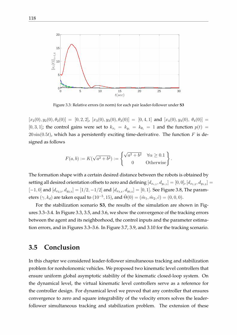
118
t(sec)0 5 10 15 20 25 30
‖ei(t)‖i=
1,4
0
5
10
15
20
Figure 3.3: Relative errors (in norm) for each pair leader-follower under S3
[x2(0), y2(0), θ2(0)] = [0, 2, 2], [x3(0), y3(0), θ3(0)] = [0, 4, 1] and [x4(0), y4(0), θ4(0)] =
[0, 3, 1]; the control gains were set to kxi = kyi = kθi = 1 and the function p(t) =
20 sin(0.5t), which has a persistently exciting time-derivative. The function F is de-
signed as follows
F (a, b) := K(√a2 + b2) :=
√a2 + b2 ∀α ≥ 0.1
0 Otherwise
.
The formation shape with a certain desired distance between the robots is obtained by
setting all desired orientation offsets to zero and defining [dxr,1 , dyr,1 ] = [0, 0], [dx1,2 , dy1,2 ] =
[−1, 0] and [dx2,3 , dy2,3 ] = [1/2,−1/2] and [dx3,4 , dy3,4 ] = [0, 1]. See Figure 3.8, The param-
eters (γ, kd) are taken equal to (10−5, 15), and Θ(0) = (m1, m2, c) = (0, 0, 0).
For the stabilization scenario S3, the results of the simulation are shown in Fig-
ures 3.3–3.4. In Figure 3.3, 3.5, and 3.6, we show the convergence of the tracking errors
between the agent and its neighborhood, the control inputs and the parameter estima-
tion errors, and in Figures 3.3–3.6. In Figure 3.7, 3.9, and 3.10 for the tracking scenario.
3.5 Conclusion
In this chapter we considered leader-follower simultaneous tracking and stabilization
problem for nonholonomic vehicles. We proposed two kinematic level controllers that
ensure uniform global asymptotic stability of the kinematic closed-loop system. On
the dynamical level, the virtual kinematic level controllers serve as a reference for
the controller design. For dynamical level we proved that any controller that ensures
convergence to zero and square integrability of the velocity errors solves the leader-
follower simultaneous tracking and stabilization problem. The extension of these

Chapter 3 119
(xi)i=1,4(m)-0.5 0 0.5 1 1.5 2
(yi)i=
1,4(m
)
-1
0
1
2
3
4
Figure 3.4: Illustration of the path-tracking in formation under S3
t(sec)0 1 2 3 4 5 6 7 8 9 10
τi(t)
i=1,4
-400
-200
0
200
400
600
Figure 3.5: Illustration of the torque inputs for each agent under S3
t(sec)0 1 2 3 4 5 6 7 8 9 10
∥ ∥ ∥Θ
i∥ ∥ ∥
i=1,4
0.702
0.7025
0.703
0.7035
0.704
Figure 3.6: Illustration of the estimation parameter errors for each agent under S3
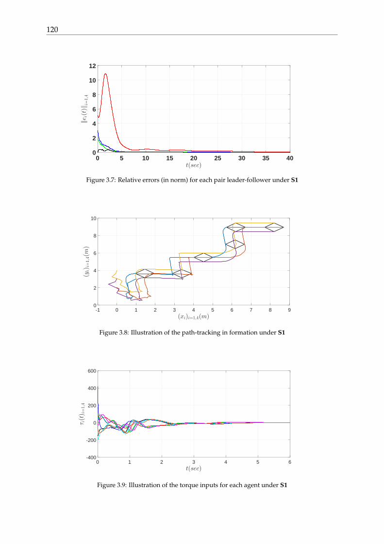
120
t(sec)0 5 10 15 20 25 30 35 40
‖ei(t)‖ i
=1,4
0
2
4
6
8
10
12
Figure 3.7: Relative errors (in norm) for each pair leader-follower under S1
(xi)i=1,4(m)-1 0 1 2 3 4 5 6 7 8 9
(yi)i=
1,4(m
)
0
2
4
6
8
10
Figure 3.8: Illustration of the path-tracking in formation under S1
t(sec)0 1 2 3 4 5 6
τi(t)
i=1,4
-400
-200
0
200
400
600
Figure 3.9: Illustration of the torque inputs for each agent under S1

Chapter 3 121
t(sec)0 1 2 3 4 5 6 7 8 9 10
∥ ∥ ∥Θ
i∥ ∥ ∥
i=1,4
0.702
0.7025
0.703
0.7035
0.704
Figure 3.10: Illustration of the estimation parameter errors for each agent under S1
results to leader-follower simultaneous tracking and agreement formation problem,
presented in Section 3.3, is based on the controller design from Section 3.2 and ensures
asymptotic convergence of the formation errors under a spanning tree communication
graph topology.

122

Chapter 4
Consensus-based formation control of
nonholonomic robots under delayed
interconnections
In previous chapters we addressed several problems on leader-follower formation
control for swarms of mobile robots under two standing assumptions:(i) the commu-
nication is reliable (notably, without delay) and (ii) the communication topology is re-
stricted to that of a spanning tree. On the other hand, the existence of a leader system
that imposes particular behaviors to the formation imposes certain technical difficul-
ties. In this chapter we restrict our attention to the leaderless consensus problem of
multiple mobile robots, but under the assumption that the robots are interconnected
in a general bidirectional graph and that the communications are affected by time-
varying delays.
As we have mentioned in previous chapters, one of the main difficulties appear-
ing in the formation control of nonholonomic systems is that the designed controller
has to be either discontinuous or time-varying [15]. Different approaches have been
proposed to deal with consensus-like control objectives. For instance, in [24] a decen-
tralized feedback control is introduced that drives a system of multiple nonholonomic
unicycles to a rendezvous point in terms of both position and orientation, the proposed
control law is discontinuous and time-invariant. In [55] necessary and sufficient con-
ditions for the feasibility of a class of position formations are presented. In [100] a dis-
tributed formation control law using a consensus-based approach is proposed to drive
a group of agents to a desired geometric pattern. In [121] the position/orientation
formation control problem for multiple nonholonomic agents using a time-varying
controller that leads the agents to a given formation using only their orientation is ad-
dressed. To solve the consensus and formation-control problems, in [31] a cooperative
123
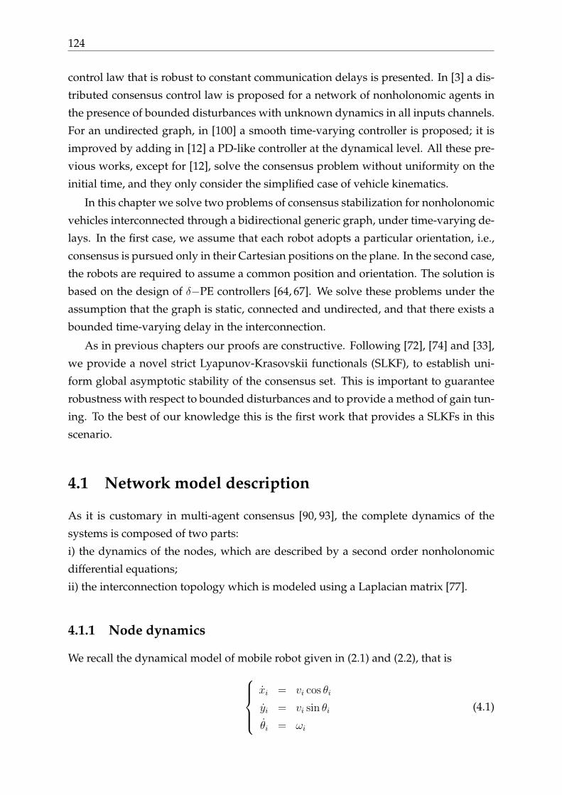
124
control law that is robust to constant communication delays is presented. In [3] a dis-
tributed consensus control law is proposed for a network of nonholonomic agents in
the presence of bounded disturbances with unknown dynamics in all inputs channels.
For an undirected graph, in [100] a smooth time-varying controller is proposed; it is
improved by adding in [12] a PD-like controller at the dynamical level. All these pre-
vious works, except for [12], solve the consensus problem without uniformity on the
initial time, and they only consider the simplified case of vehicle kinematics.
In this chapter we solve two problems of consensus stabilization for nonholonomic
vehicles interconnected through a bidirectional generic graph, under time-varying de-
lays. In the first case, we assume that each robot adopts a particular orientation, i.e.,
consensus is pursued only in their Cartesian positions on the plane. In the second case,
the robots are required to assume a common position and orientation. The solution is
based on the design of δ−PE controllers [64, 67]. We solve these problems under the
assumption that the graph is static, connected and undirected, and that there exists a
bounded time-varying delay in the interconnection.
As in previous chapters our proofs are constructive. Following [72], [74] and [33],
we provide a novel strict Lyapunov-Krasovskii functionals (SLKF), to establish uni-
form global asymptotic stability of the consensus set. This is important to guarantee
robustness with respect to bounded disturbances and to provide a method of gain tun-
ing. To the best of our knowledge this is the first work that provides a SLKFs in this
scenario.
4.1 Network model description
As it is customary in multi-agent consensus [90, 93], the complete dynamics of the
systems is composed of two parts:
i) the dynamics of the nodes, which are described by a second order nonholonomic
differential equations;
ii) the interconnection topology which is modeled using a Laplacian matrix [77].
4.1.1 Node dynamics
We recall the dynamical model of mobile robot given in (2.1) and (2.2), that isxi = vi cos θi
yi = vi sin θi
θi = ωi
(4.1)

Chapter 4 125
vi = f1(t, vi, ωi, zi) + g1(t, vi, ωi, zi)u1i
ωi = f2(t, vi, ωi, zi) + g2(t, vi, ωi, zi)u2i
(4.2)
Assuming that g1(t, vi, ωi, qi) and g2(t, vi, ωi, qi) are invertible and using the complete
knowledge of the system states and parameters, let
u1i =g1(t, vi, ωi, zi)−uvi − f1(t, vi, ωi, zi),
u2i =g2(t, vi, ωi, zi)−uωi − f2(t, vi, ωi, zi)
so that we obtain the familiar second-order modelxi = vi cos θi
yi = vi sin θi
θi = ωi,
(4.3)
vi = uvi
ωi = uωi.(4.4)
The consensus problem consists in making each vehicle achieve a certain position rel-
ative to an unknown barycenter. In addition, the vehicles may be required to adopt a
common orientation or they may be allowed to adopt, each, a particular target orien-
tation.
In a compact form, we consider the following model of N second order nonholo-
nomic robots,
z = Φ(θ)v (4.5a)
v = uv (4.5b)
θ = ω (4.5c)
ω = uω (4.5d)
where z := [z>1 , ..., z>N ]> ∈ R2N ; zi := [xi − δxi, yi − δyi]> ∈ R2 is the translational error
of the global translational coordinates [xi, yi] ∈ R2, of the ith-robot, with respect to
a constant vector δi := [δxi, δyi]> ∈ R2; the global translational coordinates [xi, yi] are
expressed with respect to a fixed frame; the constant vector δi determines the desired
position of the ith-robot relative to the barycenter of the formation zc when zi = zc;
v := [v1, ..., vN ]> ∈ RN ; vi is the linear velocity, Φ(θ) := diag[φ(θi)] ∈ R2N×N ; φ(θi) :=
[cos(θi), sin(θi)]> ∈ R2; θ := θ − θd := [θ1 − θd1, ..., θN − θdN ]> ∈ RN is the orientation
error of each robot; θd is a constant desired orientation; ω := [ω1, ..., ωN ]> ∈ RN ; ωi is
the angular velocity; and uv := [uv1, ..., uvN ]> ∈ RN and uω := [uω1, ..., uωN ]> ∈ RN are,
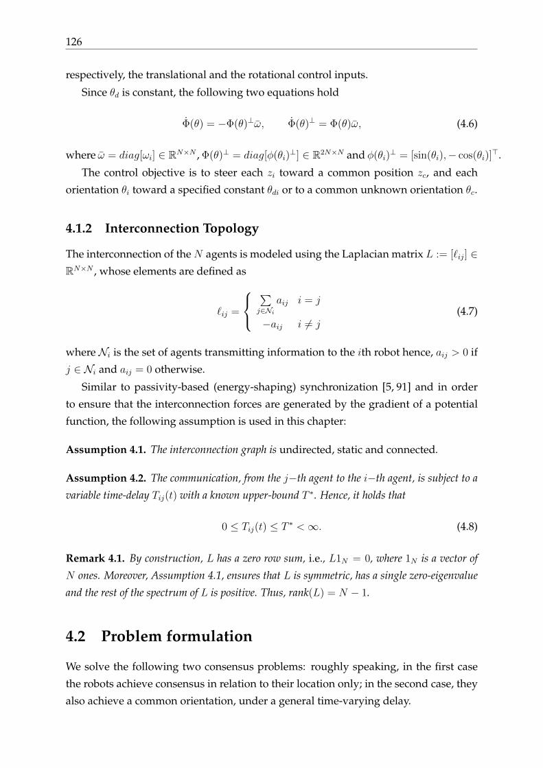
126
respectively, the translational and the rotational control inputs.
Since θd is constant, the following two equations hold
Φ(θ) = −Φ(θ)⊥ω, Φ(θ)⊥ = Φ(θ)ω, (4.6)
where ω = diag[ωi] ∈ RN×N , Φ(θ)⊥ = diag[φ(θi)⊥] ∈ R2N×N and φ(θi)
⊥ = [sin(θi),− cos(θi)]>.
The control objective is to steer each zi toward a common position zc, and each
orientation θi toward a specified constant θdi or to a common unknown orientation θc.
4.1.2 Interconnection Topology
The interconnection of the N agents is modeled using the Laplacian matrix L := [`ij] ∈RN×N , whose elements are defined as
`ij =
∑j∈Ni
aij i = j
−aij i 6= j(4.7)
where Ni is the set of agents transmitting information to the ith robot hence, aij > 0 if
j ∈ Ni and aij = 0 otherwise.
Similar to passivity-based (energy-shaping) synchronization [5, 91] and in order
to ensure that the interconnection forces are generated by the gradient of a potential
function, the following assumption is used in this chapter:
Assumption 4.1. The interconnection graph is undirected, static and connected.
Assumption 4.2. The communication, from the j−th agent to the i−th agent, is subject to a
variable time-delay Tij(t) with a known upper-bound T ∗. Hence, it holds that
0 ≤ Tij(t) ≤ T ∗ <∞. (4.8)
Remark 4.1. By construction, L has a zero row sum, i.e., L1N = 0, where 1N is a vector of
N ones. Moreover, Assumption 4.1, ensures that L is symmetric, has a single zero-eigenvalue
and the rest of the spectrum of L is positive. Thus, rank(L) = N − 1.
4.2 Problem formulation
We solve the following two consensus problems: roughly speaking, in the first case
the robots achieve consensus in relation to their location only; in the second case, they
also achieve a common orientation, under a general time-varying delay.

Chapter 4 127
Delayed Partial Consensus Problem. Consider a network of N nonholonomic
robots satisfying (4.5). Design a decentralized controller verifying Assumptions 4.1-
4.2 such that all robots positions converge, globally, uniformly, and asymptotically, to
a given formation pattern with a desired given orientation θd ∈ RN , i.e., there exists
zc ∈ R2 such that
limt→∞
z(t) = 1N ⊗ zc; (4.9a)
limt→∞
θi(t) = θdi, (4.9b)
where θdi ∈ R is a given desired constant orientation for each robot, and zc is the
barycenter of the formation pattern.
Delayed Full Consensus Problem. Consider a network of N nonholonomic robots
satisfying (4.5). Design a decentralized controller verifying Assumptions 4.1-4.2 such
that all robots positions and orientation converge, globally, uniformly, and asymptoti-
cally, to a given formation pattern, i.e., there exists [zc θc] ∈ R3 such that
limt→∞
z(t) = 1N ⊗ zc; (4.10a)
limt→∞
θi(t) = θc, (4.10b)
where [θc zc] are the barycenter of the formation pattern. As in previous chapters, we
solve the afore-mentioned consensus problems by recasting them into classical sta-
bilization problems (of the origin or of a set)1. To that end, we first need to intro-
duce suitable error coordinates (e, s) such that if (e, s) = 0 then equivalently we have
z(t) = 1N ⊗ zc.Let i ≤ n,
ei = φ(θi)>∑j∈Ni
aij(zi − zj),
si = φ(θi)⊥>∑j∈Ni
aij(zi − zj)
which, defining e := [e1 . . . eN ], s := [s1 . . . sN ], may be written in the equivalent vector
form
e =Φ(θ)>L2z, s = Φ(θ)⊥>L2z. (4.11)
On the other hand, in the presence of state delays, we introduce the delayed counter-
part of (ei, si), denoted by (edi, sdi), as
edi = φ(θi)>∑j∈Ni
aij(zj(t− Tij(t))− zi(t)),
1–see Appendix A.2 for basic definitions and characterizations of stability

128
sdi = φ(θi)⊥>∑j∈Ni
aij(zj(t− Tij(t))− zi(t)).
Correspondingly, in vector form we have
ed =Φ(θ)>L2z + Φ(θ)>A(zt),
sd =Φ(θ)⊥>L2z + Φ(θ)⊥>A(zt).(4.12)
where
A(zt) =
∑
j∈N1a1j
∫ tt−Tj1(t)
zj(δ)dδ...∑
j∈NN aNj∫ tt−TjN (t)
zj(δ)dδ
(4.13)
and we recall that L2 = L⊗ I2.
Then, the control objective (4.9a) (or (4.10a)) is achieved if we prove that (ed, sd, v)→(0, 0, 0). In fact, having v = 0, implies that A(zt) = 0 and (ed, sd) = (e, s) then, after
Lemma 4.1 below, we know that verifying the control objective (4.9a) (or (4.10a)) is
equivalent to establishing that (e, s)→ (0, 0).
Lemma 4.1. Consider (e, s) given by (4.11), and assume that L satisfies Assumption 4.1.
Then L2z = 0⇔ (e, s) = (0, 0) and, moreover,
λ2(L)z>L2z ≤ |e|2 + |s|2 ≤ λN(L)z>L2z (4.14)
where λ2(L) and λN(L) are the second smallest and the largest eigenvalue of L, respectively.
Proof. Since the matrix
[Φ(θ)>
Φ(θ)⊥>
]is non singular. The first fact follows directly. For the
second fact, we remark that |e|2 + |s|2 = z>L22z = z>L
122L2L
122 z. Since L
122 z is orthogonal
to the eigenspace associated to the zero eigenvalue of L2, it holds that
λ2(L)z>L122L
122 z ≤ z>L
122L2L
122 z ≤ λN(L)z>L
122L
122 z
so (4.14) follows.
4.3 Control design and stability analysis
Before providing the control inputs for each case-study, we introduce the following
useful functions.
First, we define the function p : R≥0 → R that satisfies the following assumption.
Chapter 4 129
Assumption 4.3. the function p : R≥0 → R and its derivatives, up to the third, are bounded.
Thus, there exists bp > 0 such that
max|p|∞, |p|∞, |p|∞, |p(3)|∞
≤ bp.
Moreover, p(t) is persistently exciting, with excitation parameters (T, µ).
Next, we define the function q : R≥0 → RN×N , as q(t) = diag(qi(t)) and which is
related to p(t) by the differential equation
q(3) +Kα ¨q +KI ˙q = pIn, (4.15)
where Kα and KI are diagonal positive definite matrices. Also, we define the function
f : R≥0 → RN×N , as f(t) := diag(fi(t)) and which is related to p(t) by the following
differential equation¨f +Kdθ
˙f +Kpθf = p(t)In, (4.16)
in which, Kdθ and Kpθ are diagonal positive definite matrices.
If p(t) satisfies Assumption 4.3 then, after Lemma B.1, it follows that fi and qi are
also persistently exciting 2 and so are the matrices ¯f(t) = ˙f(t) and ¯q(t) = ˙q(t) in the
sense of Definition A.6. Furthermore, there exist bf > 0 and bq > 0 such that
max∣∣f ∣∣∞, ∣∣ ¯f
∣∣∞,∣∣ ¯f∣∣∞,∣∣f (3)
∣∣∞
≤ bf .
and
max∣∣q∣∣∞, ∣∣¯q∣∣∞, ∣∣¯q∣∣∞, ∣∣q(3)
∣∣∞
≤ bq.
Remark 4.2. Lemma B.1 also provides an explicit estimation of the excitation parameters
(Tf , µf ) for f , (Tq, µq) for q, and the constants bf and bq, which are used in the construction of
the strict Lyapunov function.
Finally, for a bounded function ψ : R≥0 → RN , with |ψ|∞ = bψ > 0, we recall the
function Υψ2 : R≥0 → RN×N , as Υψ2(t) := diag(
Υψ2i(t))
, with
Υψ2i(t) := 1 + 2b2
ψT −2
T
∫ t+T
t
∫ m
t
ψi(s)2ds dm (4.17)
–cf equation (1.4) in Chapter 1.
Recall also that Υψ2i(t) admits the following bounds 1 ≤ Υψ2
i(t) < bΥi := 1 + 2b2
ψT
2This is reminiscent of the fact that the output of a stable proper minimum phase filter driven by aPE input is also PE –see [41, Lemma 4.8.3]

130
and, furthermore,
Υψ2i(t) = − 2
T
∫ t+T
t
ψi(s)2ds+ 2ψi(t)
2. (4.18)
Moreover, if ψ is persistently exciting, we obtain
Υψ2i(t) ≤ −2µ
T+ 2ψi(t)
2. (4.19)
We are now ready to provide the translation and the rotation control laws (uv, uω) to
solve the partial and the full delayed and undelayed consensus problems.
4.3.1 Undelayed partial consensus problem
In the translational error coordinates (e, s), we employ a simple undelayed PD-like
controller as it was originally proposed in [12], that is,
uv = −Kdtv −Kpte, (4.20)
where Kdt and Kpt are diagonal positive definite matrices. For the rotational part, we
propose the following controller
uω = −Kdθω −Kpθθ − p(t)κ(s, e) (4.21)
where Kdθ and Kpθ are diagonal positive definite matrices, and κ(s, e) is defined as
κ(s, e) =1
2[s2
1 + e21, ..., s
2N + e2
N ]> ∈ RN . (4.22)
The closed-loop system, which results from Equations (4.5), (4.11), (4.20), and (4.21), is
z =Φ(θ)v (4.23a)
v =−Kdtv −Kpte (4.23b)
e =− ωs+ Φ(θ)>L2Φ(θ)v (4.23c)
s =ωe+ Φ(θ)⊥>L2Φ(θ)v (4.23d)˙θ =ω (4.23e)
ω =−Kdθω −Kpθθ − p(t)κ(s, e). (4.23f)
Thus, equations (4.23a)-(4.23b) determine the closed-loop dynamics for the transla-
tional dynamics while equations (4.23e)-(4.23f) determines the closed-loop dynamics
of the rotational coordinates (θ, ω). These can be viewed as a stable second order sys-

Chapter 4 131
tem with input −p(t)κ(s, e) whose role is to excite the rotational velocity ω when the
errors (s, e) are different from zero.
We establish uniform global asymptotic stability of the origin of the system (4.23).
Our proof is constructive as it relies on the construction of a strict Lyapunov function.
To that end, we introduce the following change of coordinates:
eθ = θ + f(t)κ(s, e), eω = ω + ˙f(t)κ(s, e). (4.24)
Next, let us define Xt := [v>, e>, s>]> ∈ R3N and Xr := [e>θ , e>ω ]> ∈ R2N as the trans-
lational and the rotational components of the system, respectively. Additionally, let
e = diag(ei), s = diag(si), eω = diag(eωi) and κ = diag(κi). Then using (4.16), we
obtain
Xt =
−Kdt −Kpt 0
0 0 ˙fκ− eω0 − ˙fκ+ eω 0
Xt +
0
Φ>L2
Φ⊥>L2
Φv (4.25a)
Xr =
[0 IN
−Kpθ −Kdθ
]Xr +
[f˙f
] (eΦ>L2 + sΦ⊥>L2
)Φv. (4.25b)
We remark that in view of Lemma 4.1, (Xt, Xr) = (0, 0) is equivalent to (v, z, θ, ω) =
(0, 1N ⊗ zc, θd, 0), and the dynamics (4.23) is embedded in (4.25). Thus, solving the
consensus problem is equivalent to proving uniform global asymptotic stability of the
origin for (4.25).
Theorem 4.1. Consider the system (4.5) in closed-loop with (4.20) and (4.21). Assume that
Kdt, Kpt, Kdθ and Kpθ are diagonal positive definite and Assumption 4.3 holds. Then, the
origin (Xt, θ, ω) = (0, 0, 0) is uniformally globally asymptotically stable.
Proof. (Sketch) The proof is constructive; we provide a strict Lyapunov function. Only
the main steps are given here, the complete proof is in Appendix B.9.
First, we observe that (4.25a) admits the following non-strict Lyapunov function
V (v, z) = v>K−1pt v + z>L2z. (4.26)
Indeed, in view of (4.14), it is concluded that V (v, z) is positive definite and radially
unbounded with regards to Xt = 0, and using (4.14) we obtain
v>K−1pt v +
1
λN(L)
(eT e+ sT s
)≤ V (v, z) ≤ v>K−1
pt v +1
λ2(L)
(eT e+ sT s
).
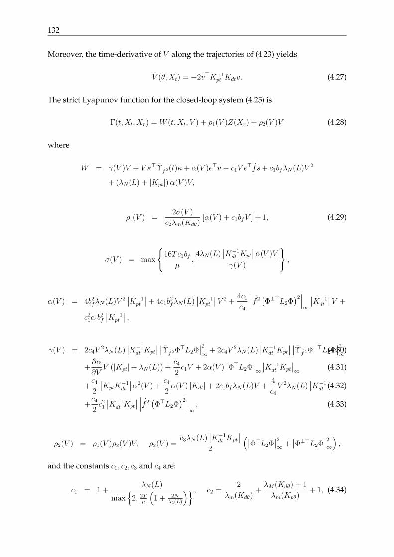
132
Moreover, the time-derivative of V along the trajectories of (4.23) yields
V (θ,Xt) = −2v>K−1pt Kdtv. (4.27)
The strict Lyapunov function for the closed-loop system (4.25) is
Γ(t,Xt, Xr) = W (t,Xt, V ) + ρ1(V )Z(Xr) + ρ2(V )V (4.28)
where
W = γ(V )V + V κ>Υf2(t)κ+ α(V )e>v − c1V e> ¯fs+ c1bfλN(L)V 2
+ (λN(L) + |Kpt|)α(V )V,
ρ1(V ) =2σ(V )
c2λm(Kdθ)[α(V ) + c1bfV ] + 1, (4.29)
σ(V ) = max
16Tc1bf
µ,4λN(L)
∣∣K−1dt Kpt
∣∣α(V )V
γ(V )
,
α(V ) = 4b2fλN(L)V 2
∣∣K−1pt
∣∣+ 4c1b2fλN(L)
∣∣K−1pt
∣∣V 2 +4c1
c4
∣∣∣ ˙f 2(Φ⊥>L2Φ
)2∣∣∣∞
∣∣K−1dt
∣∣V +
c21c4b
2f
∣∣K−1pt
∣∣ ,γ(V ) = 2c4V
2λN(L)∣∣K−1
dt Kpt
∣∣ ∣∣Υf2Φ>L2Φ∣∣2∞ + 2c4V
2λN(L)∣∣K−1
dt Kpt
∣∣ ∣∣Υf2Φ⊥>L2Φ∣∣2∞(4.30)
+∂α
∂VV (|Kpt|+ λN(L)) +
c4
2c1V + 2α(V )
∣∣Φ>L2Φ∣∣∞
∣∣K−1dt Kpt
∣∣∞ (4.31)
+c4
2
∣∣KptK−1dt
∣∣α2(V ) +c4
2α(V ) |Kdt|+ 2c1bfλN(L)V +
4
c4
V 2λN(L)∣∣K−1
dt
∣∣(4.32)
+c4
2c2
1
∣∣K−1dt Kpt
∣∣ ∣∣∣ ˙f 2(Φ>L2Φ
)2∣∣∣∞, (4.33)
ρ2(V ) = ρ1(V )ρ3(V )V, ρ3(V ) =c3λN(L)
∣∣K−1dt Kpt
∣∣2
(∣∣Φ>L2Φ∣∣2∞ +
∣∣Φ⊥>L2Φ∣∣2∞
),
and the constants c1, c2, c3 and c4 are:
c1 = 1 +λN(L)
max
2, 2Tµ
(1 + 2N
λ2(L)
) , c2 =2
λm(Kdθ)+λM(Kdθ) + 1
λm(Kpθ)+ 1, (4.34)

Chapter 4 133
c3 = max
8 (2c2bf + bf )
2
c2λm(Kdθ),8 (2c2bfλM(Kpθ) + bf )
2
λm(Kpθ)
, c4 = max
2,
2T
µ
(2 +
8N
λ2(L)
).
Since ρ1 and ρ2 are positive functions and radially unbounded, positive definite-
ness of Γ is ensured by the facts that Γ(t, 0, 0) = 0, for all t ≥ 0, and
W ≥ γ(V )V,
W ≤ γ(V )V + V κ>(e, s)Υf2(t)κ(e, s) + 2c1bfλN(L)V 2
+2 (λN(L) + |Kpt|)α(V )V,
Z ≥ min 1, λm(Kpθ)(e>θ eθ + e>ω eω
),
Z ≤ max 1 + c2, c2λM(Kpθ) + 1(e>θ eθ + e>ω eω
).
After some term chasing and long cumbersome manipulations we get
Γ ≤− µ
4TV 3 − ρ1(V )
8
[c2e>ωKdθeω + e>θ Kpθeθ
]− 1
4γ(V )v>KdtK
−1pt v −
1
8α(V )e>Kpte.
(4.35)
Therefore Γ is negative definite and Γ qualifies as a strict Lyapunov function for sys-
tem (4.25). Global uniform asymptotic stability of the equilibrium (Xt, Xr) = (0, 0) is
ensured and thus the consensus problem is solved.
4.3.2 Delayed partial consensus problem
Using the delayed translational error coordinates (ed, sd), we employ the following
delayed PD-like controller for the translational input
uv = −Kdtv −Kpted. (4.36)
where Kdt and Kpt are diagonal positive definite matrices.
We introduce the rotational controller as
uω = −Kdθω −Kpθθ − p(t)κ(sd, ed), (4.37)
where Kdθ and Kpθ are diagonal positive definite matrices, θ = θ− θd and the function
κ is defined in (4.22).
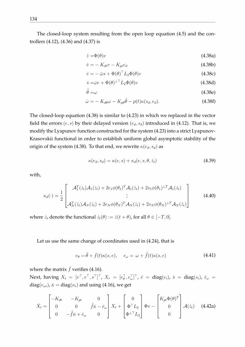
134
The closed-loop system resulting from the open loop equation (4.5) and the con-
trollers (4.12), (4.36) and (4.37) is
z =Φ(θ)v (4.38a)
v =−Kdtv −Kpted (4.38b)
e =− ωs+ Φ(θ)>L2Φ(θ)v (4.38c)
s =ωe+ Φ(θ)⊥>L2Φ(θ)v (4.38d)˙θ =ω (4.38e)
ω =−Kdθω −Kpθθ − p(t)κ(sd, ed). (4.38f)
The closed-loop equation (4.38) is similar to (4.23) in which we replaced in the vector
field the errors (e, s) by their delayed version (ed, sd) introduced in (4.12). That is, we
modify the Lyapunov function constructed for the system (4.23) into a strict Lyapunov-
Krasovskii functional in order to establish uniform global asymptotic stability of the
origin of the system (4.38). To that end, we rewrite κ(ed, sd) as
κ(ed, sd) = κ(e, s) + κd(e, s, θ, zt) (4.39)
with,
κd(·) =1
2
AT1 (zt)A1(zt) + 2e1φ(θ1)TA1(zt) + 2s1φ(θ1)⊥TA1(zt)
...
ATN(zt)AN(zt) + 2eNφ(θN)TAN(zt) + 2sNφ(θN)⊥TAN(zt)
(4.40)
where zt denote the functional zt(θ) := z(t+ θ), for all θ ∈ [−T, 0].
Let us use the same change of coordinates used in (4.24), that is
eθ = θ + f(t)κ(s, e), eω = ω + ˙f(t)κ(s, e) (4.41)
where the matrix f verifies (4.16).
Next, having Xt = [v>, e>, s>]>, Xr = [e>θ , e>ω ]>, e = diag(ei), s = diag(si), eω =
diag(eωi), κ = diag(κi) and using (4.16), we get
Xt =
−Kdt −Kpt 0
0 0 ˙fκ− eω0 − ˙fκ+ eω 0
Xt +
0
Φ>L2
Φ⊥>L2
Φv −
KptΦ(θ)T
0
0
A(zt) (4.42a)

Chapter 4 135
Xr =
[0 IN
−Kpθ −Kdθ
]Xr +
[f˙f
] (eΦ>L2 + sΦ⊥>L2
)Φv −
[0
p(t)
]κd(e, s, θ, zt). (4.42b)
The next result establishes uniform global asymptotic stability of the origin (Xt, Xr) =
(0, 0) of the system (4.42) provided that the following assumption holds
Assumption 4.4. The matrices Kdt and Kpt satisfy
1−(1 +N2a2
)T ∗λM(KptK
−dt) ≥ 0. (4.43)
Hence, we recover uniform global asymptotic stability of (v, z, θ, ω) = (0, 1N ⊗zc, θd, 0) in the original coordinates.
Theorem 4.2. Consider the system (4.5) in closed loop with (4.36) and (4.37). Assume that:
Kdt, Kpt, Kdθ and Kpθ are diagonal positive definite and Assumptions 4.1, 4.2, 4.3, 4.4 hold.
Then, the origin of the closed-loop system in the original state space, i.e, (e, s, v, θ, ω) =
(0, 0, 0, 0, 0) is uniformally globally asymptotically stable.
Proof. (Sketch) The proof is constructive; we provide a strict Lyapunov-Krasovskii
functional. Only the main steps are given here, the complete proof is in Appendix
B.10.
First, we observe that the translational part of the system admits the following non-
strict Lyapunov-Krasovskii functional
V (v, z, zt) = v>K−1pt v + z>L2z +
∫ 0
−T ∗
∫ t
t+θ
z(s)T z(s)dsdθ, (4.44)
where T ∗ = maxi,j Tij.Indeed, in view of (4.14), and the following inequality∫ 0
−T ∗
∫ t
t+θ
z(s)T z(s)dsdθ ≤ T ∗∫ t
t−T ∗|z(s)|2 ds,
it follows that the function V is positive definite and radially unbounded with respect
toXt = 0, that is, there exist two classK∞ functions u and v, such that inequality (A.10)
holds with respect to Xt = 0. Which implies that V (v, z, zt) is Lyapunov-Krasovskii
candidate with respect to Xt = 0. Moreover, the time-derivative of V along the trajec-

136
tories of (4.38) is
V =− 2v>K−1pt Kdtv + 2vTΦ(θ)TA(zt) + T ∗vTv −
∫ t
t−T ∗z(s)T z(s)ds
≤− [2− T ∗λM(KptK−dt)]v
>K−1pt Kdtv −
1
a2N
N∑j=1
N∑i=1
a2ij
∫ t
t−Tijzi(s)
T zi(s)ds
+ 2vTΦ(θ)TA(zt) (4.45)
then, we apply Jensen’s inequality∫ t
t−Tijzi(s)
T zi(s)ds ≤ −1
T ∗ij
∫ t
t−Tijzi(s)
Tds
∫ t
t−Tijzi(s)ds (4.46)
and, we use
|A(zt)|2 ≤NN∑j=1
N∑i=1
∫ t
t−Tijzi(s)
Tdsa2ij
∫ t
t−Tijzi(s)ds (4.47)
to obtain
V ≤− [2− T ∗λM(KptK−dt)]v
>K−1pt Kdtv −
1
a2NT ∗
N∑j=1
N∑i=1
a2ij
∫ t
t−Tijzi(s)
Tds
∫ t
t−Tijzi(s)ds
+N
2ε
N∑j=1
N∑i=1
∫ t
t−Tijzi(s)
Tdsa2ij
∫ t
t−Tijzi(s)ds+ ελM(KptK
−dt)v
TK−1pt Kdtv. (4.48)
Taking ε = N2aT ∗ and the matrices Kdt and Kpt such that Assumption 4.4 is verified,
we get
V ≤− v>K−1pt Kdtv −
1
2a2NT ∗
N∑j=1
N∑i=1
a2ij
∫ t
t−Tijzi(s)
Tds
∫ t
t−Tijzi(s)ds (4.49)
The strict Lyapunov-Krasovskii functional for the closed-loop system (4.42) is
Γ(t,Xt, Xr, zt) = W (t,Xt, V, zt) + ρ1(V )Z(Xr) + ρ2(V )V (4.50)
where
W = γ(V )V + V κ>Υf2(t)κ+ α(V )e>v − c1V e> ¯fs+ c1bfλN(L)V 2
+ (λN(L) + |Kpt|)α(V )V,

Chapter 4 137
Z = c2
(e>ω eω + e>θ Kpθeθ
)+ e>θ eω,
ρ1(V ) =2σ(V )
c2λm(Kdθ)(α(V ) + c1bfV ) + 1 + V,
σ(V ) = max
16Tc1bf
µ,4λN(L)
∣∣K−1dt Kpt
∣∣α(V )V
γ(V )
,
α(V ) = 4b2fλN(L)V 2
∣∣K−1pt
∣∣+ 4c1b2fλN(L)
∣∣K−1pt
∣∣V 2 +4c1
c4
∣∣∣ ˙f 2(Φ⊥>L2Φ
)2∣∣∣∞
∣∣K−1dt
∣∣V+c2
1c4b2f
∣∣K−1pt
∣∣ ,γ(V ) = 2c4V
2λN(L)∣∣K−1
dt Kpt
∣∣ ∣∣Υf2Φ>L2Φ∣∣2∞ + 2c4V
2λN(L)∣∣K−1
dt Kpt
∣∣ ∣∣Υf2Φ⊥>L2Φ∣∣2∞
+∂α
∂VV (|Kpt|+ λN(L)) +
c4
2c1V + 2α(V )
∣∣Φ>L2Φ∣∣∞
∣∣K−1dt Kpt
∣∣∞
+c4
2
∣∣KptK−1dt
∣∣α2(V ) +c4
2α(V ) |Kdt|+ 2c1bfλN(L)V +
4
c4
V 2λN(L)∣∣K−1
dt
∣∣+c4
2c2
1
∣∣K−1dt Kpt
∣∣ ∣∣∣ ˙f 2(Φ>L2Φ
)2∣∣∣∞
+ 8a2N2T ∗λM(Kpt)α(V ),
ρ2(V ) = bpρ1(V )[1 + c2]N2a2T ∗[λN(L)c5V + c6ρ1(V )] + ρ1(V )ρ3(V )V,
ρ3(V ) =c3λN(L)
∣∣K−1dt Kpt
∣∣2
(∣∣Φ>L2Φ∣∣2∞ +
∣∣Φ⊥>L2Φ∣∣2∞
),
and the constants c1, c2, c3, c4, c5 and c6 are:
c1 = 1 +λN(L)
max
2, 2Tµ
(1 + 2N
λ2(L)
) , c2 =2
λm(Kdθ)+λM(Kdθ) + 1
λm(Kpθ)+ 1,
c3 = max
8 (2c2bf + bf )
2
c2λm(Kdθ),8 (2c2bfλM(Kpθ) + bf )
2
λm(Kpθ)
,
c4 = max
2,
2T
µ
(2 +
8N
λ2(L)
), c5 =
bpN2a2T ∗[1 + c2]
min 1, λm(Kdθ),
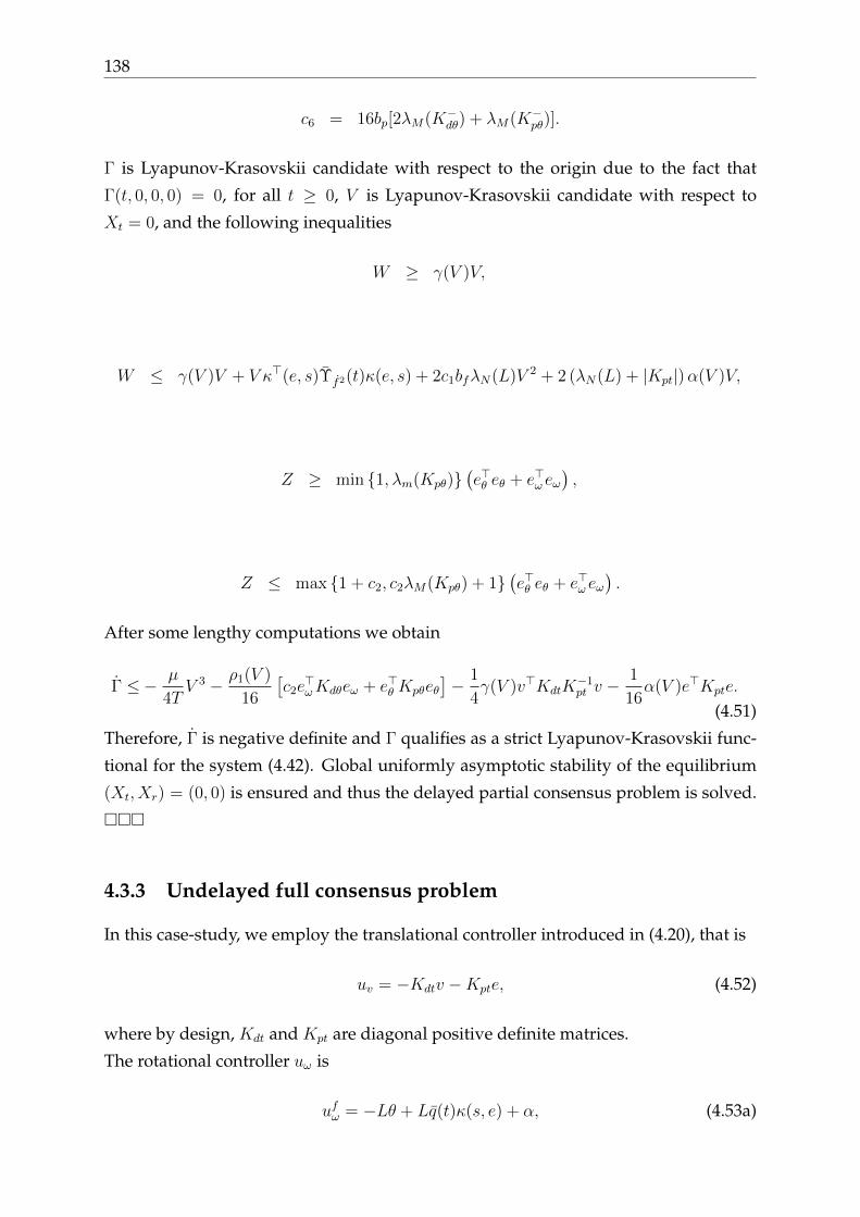
138
c6 = 16bp[2λM(K−dθ) + λM(K−pθ)].
Γ is Lyapunov-Krasovskii candidate with respect to the origin due to the fact that
Γ(t, 0, 0, 0) = 0, for all t ≥ 0, V is Lyapunov-Krasovskii candidate with respect to
Xt = 0, and the following inequalities
W ≥ γ(V )V,
W ≤ γ(V )V + V κ>(e, s)Υf2(t)κ(e, s) + 2c1bfλN(L)V 2 + 2 (λN(L) + |Kpt|)α(V )V,
Z ≥ min 1, λm(Kpθ)(e>θ eθ + e>ω eω
),
Z ≤ max 1 + c2, c2λM(Kpθ) + 1(e>θ eθ + e>ω eω
).
After some lengthy computations we obtain
Γ ≤− µ
4TV 3 − ρ1(V )
16
[c2e>ωKdθeω + e>θ Kpθeθ
]− 1
4γ(V )v>KdtK
−1pt v −
1
16α(V )e>Kpte.
(4.51)
Therefore, Γ is negative definite and Γ qualifies as a strict Lyapunov-Krasovskii func-
tional for the system (4.42). Global uniformly asymptotic stability of the equilibrium
(Xt, Xr) = (0, 0) is ensured and thus the delayed partial consensus problem is solved.
4.3.3 Undelayed full consensus problem
In this case-study, we employ the translational controller introduced in (4.20), that is
uv = −Kdtv −Kpte, (4.52)
where by design, Kdt and Kpt are diagonal positive definite matrices.
The rotational controller uω is
ufω = −Lθ + Lq(t)κ(s, e) + α, (4.53a)
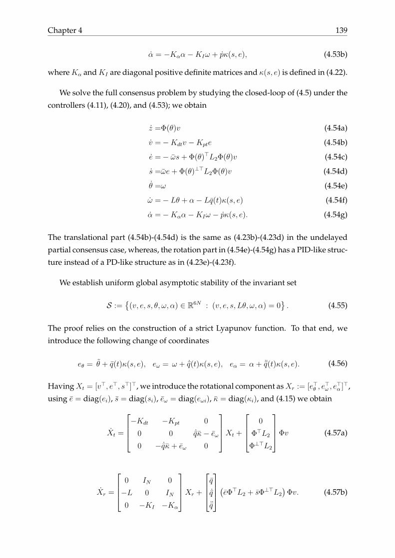
Chapter 4 139
α = −Kαα−KIω + pκ(s, e), (4.53b)
whereKα andKI are diagonal positive definite matrices and κ(s, e) is defined in (4.22).
We solve the full consensus problem by studying the closed-loop of (4.5) under the
controllers (4.11), (4.20), and (4.53); we obtain
z =Φ(θ)v (4.54a)
v =−Kdtv −Kpte (4.54b)
e =− ωs+ Φ(θ)>L2Φ(θ)v (4.54c)
s =ωe+ Φ(θ)⊥>L2Φ(θ)v (4.54d)
θ =ω (4.54e)
ω =− Lθ + α− Lq(t)κ(s, e) (4.54f)
α =−Kαα−KIω − pκ(s, e). (4.54g)
The translational part (4.54b)-(4.54d) is the same as (4.23b)-(4.23d) in the undelayed
partial consensus case, whereas, the rotation part in (4.54e)-(4.54g) has a PID-like struc-
ture instead of a PD-like structure as in (4.23e)-(4.23f).
We establish uniform global asymptotic stability of the invariant set
S :=
(v, e, s, θ, ω, α) ∈ R6N : (v, e, s, Lθ, ω, α) = 0. (4.55)
The proof relies on the construction of a strict Lyapunov function. To that end, we
introduce the following change of coordinates
eθ = θ + q(t)κ(s, e), eω = ω + ˙q(t)κ(s, e), eα = α + ¨q(t)κ(s, e). (4.56)
HavingXt = [v>, e>, s>]>, we introduce the rotational component asXr := [e>θ , e>ω , e
>α ]>,
using e = diag(ei), s = diag(si), eω = diag(eωi), κ = diag(κi), and (4.15) we obtain
Xt =
−Kdt −Kpt 0
0 0 ˙qκ− eω0 − ˙qκ+ eω 0
Xt +
0
Φ>L2
Φ⊥>L2
Φv (4.57a)
Xr =
0 IN 0
−L 0 IN
0 −KI −Kα
Xr +
q
˙q
¨q
(eΦ>L2 + sΦ⊥>L2
)Φv. (4.57b)

140
Let us introduce the following set
D :=
(Xt, Xr) ∈ R6N : (Xt, Leθ, eω, eα) = 0. (4.58)
Note that in view of Lemma 4.1, (Xt, Xr) ∈ D is equivalent to having (v, z, θ, ω, α)
belonging to the set S introduced in (4.55). Thus, in the following, we analyze the
stability of the set D.
Theorem 4.3. Consider the system (4.5) in closed-loop with (4.20) and (4.53). Assume that
Kdt, Kpt, KI and Kα are diagonal positive definite and Assumption 4.3 holds. Then, the set Dof the closed-loop state space is uniformally globally asymptotically stable. Moreover, the proof
is constructive; we provide a strict Lyapunov function.
Proof. (Sketch) The complete proof is in Appendix B.11, here we include only the main
steps.
First, the translational part of the system admits V (v, z) as a non-strict Lyapunov
function, using (4.26) and (4.27) and the fact that the translational part is the same in
(4.57) and in (4.25).
The strict Lyapunov function for the closed-loop system (4.57) is
Γ(t,Xt, Xr) = W (t,Xt, V ) + ρ1(V )Z(Xr) + ρ2(V )V (4.59)
where
W = γ(V )V + V κ>Υq2(t)κ+ α(V )e>v − c1V e> ¯qs+ c1bqλN(L)V 2
+ (λN(L) + |Kpt|)α(V )V,
Z = c2
(eTθ Leθ + eTωeω + eTαK
−I eα
)+ c5e
Tωeα + eTθ Leω,
ρ1(V ) =2σ(V )
c5λm(KI)(α(V ) + c1bqV ) + 1, (4.60)
σ(V ) = max
16Tc1bq
µ,4λN(L)
∣∣K−1dt Kpt
∣∣α(V )V
γ(V )
, (4.61)
α(V ) = 4b2qλN(L)V 2
∣∣K−1pt
∣∣+ 4c1b2qλN(L)
∣∣K−1pt
∣∣V 2 +4c1
c4
∣∣∣¯q2(Φ⊥>L2Φ
)2∣∣∣∞
∣∣K−1dt
∣∣V+c2
1c4b2q
∣∣K−1pt
∣∣ ,

Chapter 4 141
γ(V ) = 2c4V2λN(L)
∣∣K−1dt Kpt
∣∣ ∣∣Υq2Φ>L2Φ∣∣2∞ + 2c4V
2λN(L)∣∣K−1
dt Kpt
∣∣ ∣∣Υq2Φ⊥>L2Φ∣∣2∞
+∂α
∂VV (|Kpt|+ λN(L)) +
c4
2c1V + 2α(V )
∣∣Φ>L2Φ∣∣∞
∣∣K−1dt Kpt
∣∣∞
+c4
2
∣∣KptK−1dt
∣∣α2(V ) +c4
2α(V ) |Kdt|+ 2c1bqλN(L)V +
4
c4
V 2λN(L)∣∣K−1
dt
∣∣+c4
2c2
1
∣∣K−1dt Kpt
∣∣ ∣∣∣¯q2(Φ>L2Φ
)2∣∣∣∞,
ρ2(V ) = c3ρ3(V ), ρ3(V ) = V ρ1(V )λn(L)[∣∣φTLφ∣∣∞ +
∣∣φ⊥TLφ∣∣∞] , (4.62)
and the constants c1, c2, c3 and c4 are:
c1 = 1 +λN(L)
max
2, 2Tµ
(1 + 2N
λ2(L)
) ,
c2 = 4c5λ(KIKα) + 4c5λM(K2IKα) + 4c2
5λM(KIK−α )
+ 4λM(KIK−α ) + 2λn(L) + 4 + 2λM(KI)c
25,
c3 = 2b2q
[(2c2 + 1)2 +
λM(K−I )
c5
(2c2 + c5 + λn(L))2+
λM(K−αKI)
c2
(2λM(K−I ) + c5)2
] ∣∣K−dtKpt
∣∣ ,
c4 = max
2,
2T
µ
(2 +
8N
λ2(L)
), c5 = 4λn(L)λM(K−I ).
Positive definiteness of Γ with respect toD is ensured, which means that Γ(t,Xt, Xr) ≥0 and Γ(t,Xt, Xr) = 0 ⇔ |[Xt Xr]|D, for all t ≥ 0), using the fact that ρ1 and ρ2 are
positive radially unbounded functions and the following inequalities hold
W ≥ γ(V )V,
W ≤ γ(V )V + V κ>(e, s)Υq2(t)κ(e, s) + 2c1bfλN(L)V 2 + 2 (λN(L) + |Kpt|)α(V )V,
and
c2
2
(eTθ Leθ + eTωeω + eTαK
−I eα
)≤ Z ≤ 2c2
(eTθ Leθ + eTωeω + eTαK
−I eα
).

142
After some term chasing and some cumbersome manipulations we get
Γ ≤− ρ1(V )
8
[c2e
TαK
−I Kαeα + c5e
TωKIeω + eTθ L
2eθ]
− 1
4γ(V )v>KdtK
−1pt v −
1
8α(V )e>Kpte−
µ
4TV 3
(4.63)
Therefore Γ is negative definite and Γ qualifies as a strict Lyapunov function for the
system (4.57). Global uniformly asymptotic stability of the set D is ensured and thus
the full consensus problem is solved.
4.3.4 Delayed full consensus problem
For the translational controller, we employ the same delayed PD-like controller used
in (4.36), that is,
uv = −Kdtv −Kpted. (4.64)
where Kdt and Kpt are diagonal positive definite matrices.
For the rotational part, we introduce for each i
uωi =−Kωiωi −Kωiqiκi(sd, ed)−∑j∈Ni
aij (θi − θj(t− Tij(t))) + αi
+∑j∈Ni
aij [qiκi(sd, ed)− qj(t− Tij(t))κj(sd(t− Tij(t)), ed(t− Tij(t)))] (4.65a)
αi =−Kαiαi −KIiωi + pκi(sd, ed). (4.65b)
with Kω, Kα and KI diagonal positive definite matrices.
Using the variable eθ := θ + qκ(e, s), the control law (4.65) has the following form
uω = −Kωω −Kω¯qκ(sd, ed)− (Leθ +A(eθt)) + α− (4.66a)
...∑
j∈Ni aijqi [κi(sd, ed)− κi(s, e)]...
+
...∑
j∈Ni aijqj(t− Tij)
[κj(sd(t− Tij), ed(t− Tij))−κj(s(t− Tij), e(t− Tij))
]...
,α = −Kαα−KIω + pκ(sd, ed), (4.66b)
Chapter 4 143
where
A(eθt) =
∑
j∈N1a1j
∫ tt−Tj1(t)
eθj(δ)dδ...∑
j∈NN aNj∫ tt−TjN (t)
eθj(δ)dδ
, (4.67)
Leθ +A(eθt) =
∑
j∈N1a1j(eθ1 − eθj(t− Tj1))
...∑j∈NN aNj(eθN − eθj(t− TjN))
, (4.68)
and the function κ defined in (4.22).
Using (4.39) and the matrix D := diag[∑
j∈Ni aij
], we obtain
uω = −Kωω −Kω¯qκ(sd, ed)− (Leθ +A(eθt)) + α−Dqκd(·) + B(t) (4.69a)
α = −Kαα−KIω + pκ(sd, ed). (4.69b)
where
B(t) :=
...∑
j∈Ni aijqj(t− Tij)κdj(s(t− Tij), e(t− Tij), θ(t− Tij), zt−Tij
)...
,In this part, we use the controllers (4.12), (4.36), and (4.65), in closed-loop with the
system (4.5) to obtain
z =Φ(θ)v (4.70a)
v =−Kdtv −Kpted (4.70b)
e =− ωs+ Φ(θ)>L2Φ(θ)v (4.70c)
s =ωe+ Φ(θ)⊥>L2Φ(θ)v (4.70d)
θ =ω (4.70e)
ω =−Kωω − Leθ + α−A(eθt)−Kω¯qκ(ed, sd)−Dqκd(t) + B(t) (4.70f)
α =−Kαα−KIω − pκ(sd, ed). (4.70g)
The closed-loop equation (4.70) is similar to (4.54) in which we replaced the errors (e, s)
by their delayed version (ed, sd) introduced in (4.12). In the next theorem, we propose
to extend the strict Lyapunov function constructed for the the system (4.54) to a strict
Lyapunov-Krasovskii functional in order to establish uniform global asymptotic sta-
bility of the set S introduced in (4.55) for the closed-loop system when B(·) = 0, then

144
we use the output injection argument in Lemma A.7 to conclude the global uniform
asymptotic stability of the global closed-loop system.
Remark 4.3. The output injection argument in Lemma A.7 remains valid in the presence of
uniformally bounded time delay at least when the unperturbed system admits a strict Lyapunov-
Karasovskii functional.
Let us recall the change of coordinates used in (4.56)
eθ = θ + q(t)κ(s, e), eω = ω + ˙q(t)κ(s, e), eα = α + ¨q(t)κ(s, e). (4.71)
Having Xt = [v>, e>, s>]>, Xr = [e>θ , e>ω , e
>α ]>, e = diag(ei), s = diag(si), eω = diag(eωi),
κ = diag(κi) and using (4.15), we obtain
Xt =
−Kdt −Kpt 0
0 0 ˙qκ− eω0 − ˙qκ+ eω 0
Xt +
0
Φ>L2
Φ⊥>L2
Φv −
KptΦ(θ)T
0
0
A(zt) (4.72a)
Xr =
0 IN 0
−L −Kω IN
0 −KI −Kα
Xr −
0
A(eθt)
0
+
q
˙q
¨q
(eΦ>L2 + sΦ⊥>L2
)Φv
−
0
Kω ˙q +Dq
p
κd(e, s, θ, zt) +
0
B(t)
0
. (4.72b)
Note that in view of Lemma 4.1, (Xt, Xr) belongs to the set D, introduced in (4.58), is
equivalent to having (v, e, s, θ, ω, α) belonging to the S introduced in (4.55). Thus, we
propose to study the stability of the set D, provided that the following extra assump-
tion holds
Assumption 4.5.
λm(Kω) ≥ 2T ∗2N2a2
c2
[1
6+ 2c2
],
with,
c2 = 3λM(Kω)− 2λN(L) +3
2λM(KIK
−α ).
Theorem 4.4. Consider the system (4.5) in closed-loop with (4.36) and (4.65) with B(t) = 0.
Assume thatKdt,Kpt,Kω,Kα andKI are diagonal positive definite and Assumptions 4.1, 4.2,

Chapter 4 145
4.3, 4.5 hold. Then, the setD, introduced in (4.58), of the closed-loop state space is uniformally
globally asymptotically stable.
Proof. (Sketch) The proof is constructive; we provide a strict Lyapunov-Krasovskii
functional. The complete proof is in Appendix B.12, the main steps are the follow-
ing
First, since the translational part of the system ((4.70b)-(4.70c)) is the same as in the
partial delayed case ((4.38b)-(4.38c)) then, using (4.44) and (4.45), we conclude that it
admits V (v, z, zt) as a non-strict Lyapunov-Krasovskii functional with respect to Xt =
0.
The strict Lyapunov-Krasovskii functional for the closed-loop system (4.72) with
B(t) = 0 is
Γ(t,Xt, Xr, zt, eθt) = W (t,Xt, V, zt) + ρ1(V )Z(Xr, eθt) + ρ2(V )V (4.73)
where
W = γ(V )V + V κ>Υq2(t)κ+ α(V )e>v − c1V e> ¯qs+ c1bqλN(L)V 2
+ (λN(L) + |Kpt|)α(V )V,
Z = c2
(eTθ Leθ + eTωeω + eTαK
−I eα
)+ eTθ Leω + c5
∫ 0
−T ∗
∫ t
t+h
eTθ (s)eθ(s)dsdh,
ρ1(V ) =2σ(V )
c2λm(Kω)(α(V ) + c1bqV ) + 1 + V,
σ(V ) = max
16Tc1bq
µ,4λN(L)
∣∣K−1dt Kpt
∣∣α(V )V
γ(V )
,
α(V ) = 4b2qλN(L)V 2
∣∣K−1pt
∣∣+ 4c1b2qλN(L)
∣∣K−1pt
∣∣V 2 +4c1
c4
∣∣∣¯q2(Φ⊥>L2Φ
)2∣∣∣∞
∣∣K−1dt
∣∣V+c2
1c4b2q
∣∣K−1pt
∣∣ ,

146
γ(V ) = 2c4V2λN(L)
∣∣K−1dt Kpt
∣∣ ∣∣Υq2Φ>L2Φ∣∣2∞ + 2c4V
2λN(L)∣∣K−1
dt Kpt
∣∣ ∣∣Υq2Φ⊥>L2Φ∣∣2∞
+∂α
∂VV (|Kpt|+ λN(L)) +
c4
2c1V + 2α(V )
∣∣Φ>L2Φ∣∣∞
∣∣K−1dt Kpt
∣∣∞
+c4
2
∣∣KptK−1dt
∣∣α2(V ) +c4
2α(V ) |Kdt|+ 2c1bqλN(L)V +
4
c4
V 2λN(L)∣∣K−1
dt
∣∣+c4
2c2
1
∣∣K−1dt Kpt
∣∣ ∣∣∣¯q2(Φ>L2Φ
)2∣∣∣∞
+ 8a2N2T ∗λM(Kpt)α(V ),
ρ2(V ) = c3ρ3(V ) + ρ1(V )bqV λm(KptK−dt)(λ2N(L) + c6c5T
∗)+
2a2N2T ∗ρ1(V )[c2
2(bq + bp)c7ρ1(V ) + c6c2bq(1 +
(1 + λM(K−ωD)
)2λM(Kω))V λN(L)+
c7
2λM(Kω)
(1 + λM(K−ωD)
)2bqρ1(V ) +
2 (1 + λM(K−ωD))2λM(Kω)
c6
λN(L)V bq
],
ρ3(V ) = V ρ1(V )λn(L)[∣∣φTLφ∣∣2∞ +
∣∣φ⊥TLφ∣∣2∞] ,and the constants c1 − c7 are:
c1 = 1 +λN(L)
max
2, 2Tµ
(1 + 2N
λ2(L)
) , c2 = 3λM(Kω) + 2λN(L) +3
2λM(KIK
−α ),
c3 = b2q
[(2c2 + 1)2 + λM(Kω)(2c2 + λn(L))2 + λM(K−αKI)4λM(K−I )2
] ∣∣K−dtKpt
∣∣ ,c4 = max
2,
2T
µ
(2 +
8N
λ2(L)
), c5 = a2N2T ∗
[1
6+ 2c2
],
c6 = 16bq
[λM(Kω) +
c5T∗
c2
+ 2 + 2λM(K−I Kα)
],
c7 = 2N2T ∗a2[bpλ
2M(Kω) + λM(K−I )bp + λM(Kω)λN(L)bq
]
Notice that the functionalZ(Xr, eθt) is a strict Lyapunov-Krasovskii functional with
respect to the set
Dr :=
(Leθ, eω, α) ∈ R3N / Leθ = eω = α = 0,

Chapter 4 147
under the assumption 4.5, for the following delayed system
Xr =
0 IN 0
−L −Kω IN
0 −KI −Kα
Xr −
0
A(eθt)
0
. (4.74)
In deed, Z(Xr, eθt) is a Lyapunov-Krasovskii candidate with respect to the set Dr due
to the following inequalities
Z ≥ c2
2
(eTθ Leθ + eTωeω + eTαK
−I eα
),
Z ≤ 2c2
(eTθ Leθ + eTωeω + eTαK
−I eα
)+ 2c5T
∗∫ t
t−T ∗|eθ(s)|2 ds
then, one can easily find the two classK∞ functions u and v such that inequality (A.10)
holds with respect to the set Dr.The time-derivative of Z(Xr, θt) along trajectories of (4.74) verifies
Z(·) =− 2c2
[eTαK
−I Kαeα + eTωKωeω
]− eTθ L2eθ − eTθ LKωeω + eTθ Leα + eTωLeω
− eTθ LA(eθt)− 2c2eTωA(eθt) + c5T
∗eTθ eθ − c5
∫ t
t−T ∗eTθ (s)eθ(s)ds. (4.75)
Using the fact that Kω > IN both with the following inequalities
eTθ Leα ≤1
2εeTθ L
2eθ +ε
2λM(KIK
−α )eTαK
−I Kαeα
eTωLeω ≤ λN(L)eTωKωeω,
−2c2eTωA(eθt) ≤ ε1c2e
TωKωeω +
c2
ε1|A(eθt)|2 ,
eTθ LA(eθt) ≤1
2εeTθ L
2eθ +ε
2|A(eθt)|2 ,
eTθ LKωeω ≤1
2εeTθ L
2eθ +ελM(Kω)
2,
|A(eθt)|2 ≤ N
N∑j=1
N∑i=1
(∫ t
t−Tijeθj(s)ds
)2
a2ij,
148
∫ t
t−T ∗eTθ (s)eθ(s)ds ≥
1
a2N
N∑j=1
N∑i=1
a2ij
∫ t
t−Tije2θj(s)ds,
∫ t
t−Tija2ij e
2θj(s)ds ≥
1
T ∗
(∫ t
t−Tijeθj(s)ds
)2
a2ij,
taking ε1 = 12, ε = 3 and using Assumption 4.5 we obtain
Z(·) =− 1
2c2
[eTαK
−I Kαeα + eTωKωeω
]− 1
2eTθ L
2eθ. (4.76)
Since V and Z are Lyapunov-Krasovskii candidates with respect to Xt = 0 and Drrespectively, then we conclude that Γ is so with respect to D using the following in-
equalities.
W ≥ γ(V )V,
W ≤ γ(V )V + V κ>(e, s)Υq2(t)κ(e, s) + 2c1bfλN(L)V 2 + 2 (λN(L) + |Kpt|)α(V )V.
Then, one can easily find the two class K∞ functions u and v such that equation (A.10)
holds with respect to the set D since it verifies D = Xt = 0 ∩ Dr.After some term chasing and some cumbersome manipulations we get
Γ ≤− ρ1(V )
8
[c2e
TαK
−I Kαeα + c2e
TωKωeω + eTθ L
2eθ]
− 1
4γ(V )v>KdtK
−1pt v −
1
16α(V )e>Kpte−
µ
4TV 3.
(4.77)
This implies that Γ is negative definite and Γ qualifies as a strict Lyapunov-Krasovskii
functional for system (4.72). Global uniformly asymptotic stability of the set D is en-
sured and thus the full delayed consensus problem is solved.
Corollary 4.1. Assume that Kdt, Kpt, Kω, Kα and KI are diagonal positive definite matrices
and let Assumptions 4.1, 4.2, 4.3, 4.5 hold. Then, for the closed-loop system (4.72) the set
D, introduced in (4.58), of the closed-loop state space is uniformally globally asymptotically
stable.
Proof. The proof of the corollary is a direct application of Lemma A.7. Indeed,
Item 1. the global closed-loop system (4.72) is uniformally globally stable, that is,
using the non strict Lyapunov-Karasovskii functional V introduced in (4.44) with a
time derivative along trajectories of (4.72a) given in (4.49), which concludes the uni-

Chapter 4 149
form global stability of translational coordinates. The rotational part in (4.72b) is com-
posed by the uniformally exponentially stable linear delayed system
Xr =
0 IN 0
−L −Kω IN
0 −KI −Kα
Xr −
0
A(eθt)
0
which is ISS with respect to the bounded perturbation vector
q
¯q
¯q
(eΦ>L2 + sΦ⊥>L2
)Φv −
0
Kω¯q +Dq
p
κd(e, s, θ, zt) +
0
B(t)
0
that depends on the translational coordinates thus, the first item follows.
Item 2. the uniform global asymptotic stability of the unperturbed (system (4.72)
with B(·) = 0) follows for theorem 4.4.
Item 3. the last condition to verify concerns the integrability of the vector B(·),
having
|B(t)|2 ≤N∑i=1
(∑j∈Ni
aijqj(t− Tij)κdj(t− Tij)
)2
≤ N
N∑i=1
∑j∈Ni
a2ijqj(t− Tij)2κdj(t− Tij)2
≤Na2 |q|2∞N∑j=1
κ2dj(t− T ∗j ) (4.78)
where
T ∗j (t) := argmaxi
κ2dj(t− Tij(t))
.
Using (4.40) we obtain
κ2dj(t− T ∗j ) ≤
∣∣gj(t− T ∗j )∣∣ATj (zt−T ∗j )Aj(zt−T ∗j )
with
gj(t) =1
4
[Aj(zt) + 2ejφ(θj) + 2sjφ(θj)
⊥] [ATj (zt) + 2ejφ(θj)T + 2sjφ(θj)
⊥T ] .
150
Using (4.13) we obtain the following inequality
ATj (zt−T ∗j )Aj(zt−T ∗j ) ≤
∑k∈Nj
akj
∫ t−T ∗j
t−Tkj−T ∗jzj(δ)
Tdδ
T ∑k∈Nj
akj
∫ t−T ∗j
t−Tkj−T ∗jzj(δ)
Tdδ
≤N
∑k∈Nj
a2kj
∫ t−T ∗j
t−Tkj−T ∗jzj(δ)
Tdδ
∫ t−T ∗j
t−Tkj−T ∗jzj(δ)dδ.
From the last inequalities, we obtain
|B(·)|2 ≤N2a2 |q|2∞N∑j=1
∣∣gj(t− T ∗j )∣∣ ∑k∈Nj
a2kj
∫ t−T ∗j
t−Tkj−T ∗jzj(δ)
Tdδ
∫ t−T ∗j
t−Tkj−T ∗jzj(δ)dδ
≤N2a2 |q|2∞ supj
∣∣gj(t− T ∗j )∣∣ N∑
j=1
∑k∈Nj
a2kj
∫ t−T ∗j
t−Tkj−T ∗jzj(δ)
Tdδ
∫ t−T ∗j
t−Tkj−T ∗jzj(δ)dδ.
Having the translational part of the closed-loop system globally bounded using the
non strict Lyapunov-Karasovskii candidate V introduced in (4.44), we conclude the
global boundedness of the term N2a2 |q|2∞ supj∣∣gj(t− T ∗j )
∣∣. Then, using the time
derivative of V along the trajectories of the translational coordinates Xt(t) in (4.49) we
conclude the uniform integralbility of the term
N∑j=1
∑k∈Nj
a2kj
∫ t−T ∗j
t−Tkj−T ∗jzj(δ)
Tdδ
∫ t−T ∗j
t−Tkj−T ∗jzj(δ)dδ
since T ∗j ≤ T ∗, which conclude the proof of the corollary.
Remark 4.4. Two remarks are in order:
i) for simplicity, and without losing generality, the function p is taken equal for all the agents;
ii) the function κ in (4.22) may correspond to any class-K function with the following form
κ(sd, ed) = 12[G(s2
d1 + e2d1), ..., G(s2
dn + e2dn)]>. The only condition on κ is that there exist two
positive polynomials P1(·) and P2(·) such that:
G(·) ≤ P1(·), and,∣∣∣∣∂G(·)∂(·)
∣∣∣∣ ≤ P2(·).
4.4 Conclusion
This chapter deals with the distributed formation control of multiple nonholonomic
robots under a general time-varying delay. We report a novel decentralized consensus-
based formation controllers that consider both, the kinematic and the dynamic model
Conclusion and perspectives 151
and a delayed exchanged information between the elements of the network, to uni-
formly and asymptotically solve the partial and the full consensus problems. The net-
work is modeled as an undirected, static and connected graph. The controller has
a smooth time-varying PD-like and PID-like scheme that is δ−persistently exciting.
Up to the authors’ knowledge this is the first work that provides a strict Lyapunov
function and a strict Lyapunov-Krasovskii functional, thereby guaranteeing uniform
global asymptotic stability for the closed-loop system. Simulations, using a network
with six agents, have been provided to illustrate our theoretical contributions.

152

Conclusions & Future Work
The following concluding remarks are in order.
In Chapter 1. we presented some technical results on uniform exponential stability
of time-varying linear systems with particular structures that appear, for example,
in the analysis of model-reference adaptive systems, persistently excited observers,
consensus of systems interconnected through time-varying links and systems with
time-varying input gain. Stability proofs we presented in this section are based on the
explicit construction of strict Lyapunov functions. Such an approach allows not only
to conclude stability and convergence properties of the system trajectories but also to
give explicit decay estimates for the convergence rate.
In the subsequent chapters these stability results served as basis for the consensus
and formation control of mobile robots using controllers with persistency of excitation.
In Chapters 2-3. we identified several control problems for swarms of mobile
robots depending on nature of the leader’s velocities, notably the leader-follower track-
ing, robust agreement and simultaneous tracking-agreement problems. In all three
cases assuming a spanning tree communication graph topology, we considered two-
stage controller design – first at the kinematic and then at the dynamic level. At the
kinematics level, a nonlinear change of coordinates was used to transform the three
problems into that of uniform global asymptotic stabilization of the origin. Stability
analysis provided in these chapters relies on the extension of strict Lyapunov functions
proposed in Chapter 1, cascaded systems design, notions of iISS and strong iISS and
their characterization. In particular, we provided strict Lyapunov functions for the
closed loop systems at the kinematic level and demonstrated that at the dynamic level
one can use a variety of control schemes for Lagrangian and Hamiltonian systems that
ensure square intergrability of velocity errors.
In Chapter 4. we restricted our attention to the leaderless consensus problem of
multiple mobile robots, but under the assumption that the robots are interconnected
in a general bidirectional graph and that the communications are affected by time-
varying delays.
In particular, we considered 2 cases : in the first case, under the assumption that
153

154
each robot adopts a particular orientation, i.e., consensus is pursued only in their
Cartesian positions on the plane while in the second case, the robots required to as-
sume both common position and orientation.
We proposed decentralized smooth time-varying PD-like and PID-like controllers
that consider both, the kinematic and the dynamic models to uniformly and asymp-
totically solve the partial and the full consensus problems. Assuming that there are
no delays in the communications, we designed new strict Lyapunov function that en-
sures uniform global asymptotic stability of the consensus set, these functions served
the basis to construct strict Lyapunov-Krasovskii functional for the formation with
delays.
Although many of controllers proposed in this thesis are reminiscent of others that
have appeared in the literature, our contributions lie in the establishment of strong
properties such as uniform global asymptotic stability, (integral) intput-to-state stabil-
ity and, most remarkably, in the construction of original Lyapunov functions for most
of the control problems that we addressed.
Chapter 1 is bound to present concrete case-studies of stability analysis for time-
varying systems. Each of this case-studies, we believe, may serve as a departure point
to different lines of research. In that light, the subsequent chapters are devoted to an in-
depth study of one case-study: that of consensus and formation control of autonomous
vehicles. Other concrete open questions include:
1. Design of strict differentiable Lyapunov function for the first order time varying
consensus problem studied in Subsection 1.2.1 for the case of directed graphs.
2. Establish necessary and/or more relaxed sufficient conditions for uniform expo-
nential stability of the spiraling systems (1.51).
3. Extension of the leader-follower tracking, robust-agreement and simultaneous
tracking-agreement controllers to more general graph topologies and in the pres-
ence of time delay.
4. Extension of the results of Chapter 4 on partial and full consensus of mobile
robots to the case of connected directed graph and to other types of moving
agents.
Appendix A
Basic notions
A.1 Preliminaries
Our technical results are stability statements of nonlinear time-varying systems of the
form
x = f(t, x). (A.1)
For simplicity, we assume that f is such that solutions exist and are unique.
A.2 Uniform Stability notions
Definition A.1. Consider the time-varying dynamical system
x =f(t, x) (A.2)
where f : R≥0 × Rn → Rn is such that the solutions of (A.2) exist in finite time intervals for
all initial condition (t0, x(t0)) ∈ R× Rn and admit an invariant set A.
The invariant set A is Uniformly Stable (US) if there exist α ∈ K and r > 0, such that
|x(t, t0, x(t0))|A ≤ α(|x(t0)|A) ∀t ≥ t0, ∀ |x(t0)|A ≤ r. (A.3)
The invariant set A is Uniformly Asymptotically Stable (UAS) if there exists β ∈ KL, such
that
|x(t, t0, x(t0))|A ≤ β(t− t0, |x(t0)|A) ∀t ≥ t0, ∀ |x(t0)|A ≤ r. (A.4)
155

156
The invariant set A is Uniformly Exponentially Stable (UES) if there exists γ1, γ2 > 0, such
that
|x(t, t0, x(t0))|A ≤ γ1 |x(t0)|A e(t−t0) ∀t ≥ t0, ∀ |x(t0)|A ≤ r. (A.5)
The invariant set A is UGS, UGAS, UGES if equations (A.3), (A.4), (A.5) hold, respectively,
for all r > 0.
Definition A.2. Consider the delayed time-varying dynamical system
x =f(t, xt), t ≥ t0. (A.6)
where f : R≥0 × C[−T, 0]→ Rn is continuous in both arguments and locally Lipschitz in the
second argument. and admits an invariant set A, that is,
|x(t0 + θ)|A = 0, ∀θ ∈ [−T, 0]⇒ f(t, xt0) = 0, ∀t ≥ t0.
The invariant set A is Uniformly Stable (US) if there exist α ∈ K and r > 0, such that
|x(t, t0, xt0)|A ≤ α(|xt0|A) ∀t ≥ t0, ∀ |xt0 |A ≤ r. (A.7)
The invariant set A is Uniformly Asymptotically Stable (UAS) if there exists β ∈ KL, such
that
|x(t, t0, xt0)|A ≤ β(t− t0, |xt0|A) ∀t ≥ t0, ∀ |xt0 |A ≤ r. (A.8)
The invariant set A is Uniformly Exponentially Stable (UES) if there exists γ1, γ2 > 0, such
that
|x(t, t0, xt0)|A ≤ γ1 |xt0|A e(t−t0) ∀t ≥ t0, ∀ |xt0|A ≤ r. (A.9)
The invariant set A is UGS, UGAS, UGES if equations (A.3), (A.4), (A.5) hold, respectively,
for all r > 0.
Lemma A.1 (Lyapunov characterization). Suppose f : R≥0 × Rn → Rn; and that u; v; w
: R+ → R≥0 are continuous nondecreasing functions, u(s) and v(s) are positive for s > 0,
and u(0) = v(0) = 0. The invariant set A is uniformly stable if there exists a continuous
functional V : R≥0 × Rn → R, which is positive-definite radially unbounded with respect to
A, i.e.
u(|x(t)|A) ≤ V (t, x) ≤ v(|x|A).

Appendix A 157
and such that its derivative along (A.6) is non-positive in the sense that
V (t, x) ≤ −w(|x(t)|A).
If w(s) > 0 for s > 0, then the invariant set A solution is uniformly asymptotically stable. If
in addition lims→∞ =∞, then it is globally uniformly asymptotically stable.
Lemma A.2 (Lyapunov–Krasovskii characterization [33]). Suppose f : R≥0×C[−T, 0]→Rn; and that u; v; w : R+ → R≥0 are continuous nondecreasing functions, u(s) and v(s) are
positive for s > 0, and u(0) = v(0) = 0. The invariant set A is uniformly stable if there exists
a continuous functional V : R≥0 × W [−T, 0] × L2[−T, 0] → R, which is positive-definite
radially unbounded with respect to A, i.e.
u(|x(t)|A) ≤ V (t, xt, xt) ≤ v(‖xt‖A). (A.10)
and such that its derivative along (A.6) is non-positive in the sense that
V (t, xt, xt) ≤ −w(|x(t)|A).
If w(s) > 0 for s > 0, then the invariant set A solution is uniformly asymptotically stable. If
in addition lims→∞w(s) =∞, then it is globally uniformly asymptotically stable.
A.3 ISS and Lyapunov characterization
Definition A.3 (ISS [110]). Consider the time-varying dynamical system
x =f(t, x, u) (A.11)
where f : R≥0 × Rn × Rm → Rn, is such that its solutions exist on the infinite time interval
for all initial condition (t0, x(t0)) ∈ R× Rn and u : R≥0 → Rm.
The dynamical system (A.11) is Input-to-State Stable (ISS), with respect to the input u, if there
exists a class KL function β(·, ·), and a class K∞ function γ(·), such that:
|x(t)| ≤ β(|x(t0)| , t− t0) + γ
(sup
t0≤s≤∞|u(s)|
)(A.12)
Similarly, the dynamical system (A.11) is small Input-to-State Stable (ISS), with respect to the
input u, if there exists r > 0, such that equation (A.12) holds for |u| ≤ r.
Lemma A.3 ( [47]). Let V : [0,∞) × Rn → R be a continuously differentiable Lyapunov
158
function such that:
α (|x|) ≤ V (t,X) ≤ α (|x|) (A.13)
∂V
∂t+∂V
∂xf(t, x, u) ≤ −W (x), ∀ |x| ≥ ρ (|u|) > 0 (A.14)
Where α, α are K∞ functions, ρ a class K function, and W a continous PD function, which
implies that the system x = f(t, x, u) is ISS with respect to the input u.
Similarly, if there exists r > 0 such that (A.14) holds for |u| ≤ r then the system x = f(t, x, u)
is small ISS with respect to the input u.
A.4 integral ISS and Lyapunov characterization
Definition A.4 (Integral ISS [110]). Consider the time-varying dynamical system
x =f(t, x, u) (A.15)
where f : R≥0 × Rn × Rm → Rn, is such that its solutions exist on the infinite time interval
for all initial condition (t0, x(t0)) ∈ R× Rn and u : R≥0 → Rm.
The dynamical system (A.15) is Integral Input-to-State Stable (iISS), with respect to the input
u, if there exists a class KL function β(·, ·), and a class K∞ function γ(·), such that:
|x(t)| ≤ β(|x0| , t− t0) +
∫ t
t0
γ (|u(s)|) ds (A.16)
Lemma A.4 ( [42]). Let V : [0,∞) × Rn → R be a continuously differentiable Lyapunov
function such that:
α (|x|) ≤ V (t,X) ≤ α (|x|) (A.17)
∂V
∂t+∂V
∂xf(t, x, u) ≤ −α1(|x|) + ρ(|u|) (A.18)
Where α, α are K∞ functions, α1 a positive definite function called dissipation rate, and ρ a
class K∞ function, which implies that the system x = f(t, x, u) is integral ISS with respect to
the input u.
Appendix A 159
A.5 Strong iISS
Definition A.5 (Strong iISS [17]). Consider the time-varying dynamical system
x =f(t, x, u) (A.19)
where f : R≥0 × Rn × Rm → Rn, is such that its solutions exist on the infinite time interval
for all initial condition (t0, x0) ∈ R× Rn and u : R≥0 → Rm.
The dynamical system (A.19) is said to be strongly integral input-to-state stable (strongly
iISS) with respect to u, if it is integral input-to-state stable (iISS) with respect to u, and input-
to-state stable (ISS) with respect to sufficiently small values of u.
Lemma A.5 ( [18]). Consider the following cascaded interconnected system:
x1 =f1(t, x1, x2, u1) (A.20)
x2 =f2(t, x2, u2) (A.21)
Where f1 is strong iISS with respect to [x2 u1], and f2 is so with respect to u2, then the overall
system is strong iISS with respect to [u1 u2].
Remark A.1. The prove of the last lemma is provided in [18] for the autonomous case, but the
prove may be directly extended to the non-autonomous case, because it uses a catalog of prop-
erties introduced in [111], [8] and [9], and the crucial part when establishing these properties
uses the converse Lyapunov theorem for Asymptotic Stability which exists for the uniform
asymptotic stability,see for example [122].
A.6 Nonlinear output injection
Undelayed case
Lemma A.6 ( [99]). Consider the following system in the output injection form:
x = f(t, x) = F (t, x) +K(t, x) (A.22)
The origin of (A.22) is UGAS follows if:
i. the origin of x = f(t, x) is uniformly globally stable;
ii. the origin of x = F (t, x) is UGAS;
160
iii. there exist an ”output” y, non decreasing functions k1, k2, β: R≥0 → R≥0, and classK∞function k, as well as a positive definite function γ such that
|K(t, x)| ≤ k1(|x|)k(|y|) (A.23)
|y(t, x)| ≤ k2(|x|) (A.24)∫ ∞0
γ(|y(t)|
)≤ β(|x(0)|). (A.25)
In the presence of time varying Delay
The following lemma is the extension of Lemma A.6 to the case of time varying de-
layed systems
Lemma A.7. Consider the following delayed system in the output injection form:
x = f(t, xt) = F (t, xt) +K(t, xt) (A.26)
f : R+×C[−T, 0]→ Rn uniformly bounded in t and sufficiently smooth. The origin of (A.26)
is UGAS follows if:
i. the origin of x = f(t, xt) is UGS;
ii. the origin of x = F (t, xt) is UGAS and admits a strict differentiable Lyapunov-Karasovskii
functional continuous functional V : R+ ×W [−T, 0]× L2[−T, 0] → R with the prop-
erties
α(|x|) ≤ V (t, xt, xt) ≤ α(‖xt‖) (A.27)
VF (t, xt, xt) ≤ −α(|x|) (A.28)∣∣∣∂V (t,xt,xt)∂x
∣∣∣ ≤ α∂(‖xt‖) (A.29)
where the functions α, α, α, α∂ ∈ K∞.
iii. there exist an ”output” y : R+ × C[−T, 0] → Rm, non decreasing functions k1, k2,
β: R≥0 → R≥0, and class K∞ function k, as well as a positive definite function γ such
that
|K(t, xt)| ≤ k1(|xt|)k(|y|) (A.30)
|y(t, xt)| ≤ k2(|xt|) (A.31)∫ ∞−T
γ(|y(t, xt)|
)≤ β(|xt(0)|). (A.32)

Appendix A 161
Proof. Since the system x = F (t, xt) is UGAS, and admits a continuously differentiable
Lyaunov-Karasovskii functional V (t, xt, xt).
Taking the derivative of V (t, x) along the trajectories of A.26 we obtain
VA.26(t, xt, xt) ≤ −α(|x|) + α∂(‖xt‖)k1(|xt|)k(|y|), (A.33)
and since the system is UGS, there exist γw ∈ K∞ such that
|x(t)| ≤ γw(|xt0|), ∀t ≥ t0.
Moreover, f(t, xt) uniformly bounded in t and continuous in xt with f(t, 0) = 0 then,
there exist a class K function κ : R+ → R+ and a nondecreasing function µ : R+ → R+
such that
‖xt‖ ≤ κ (|xt0|) , ∀t ≥ t0 + T
and
α∂(‖xt‖)k1(|xt|) ≤ µ(|xt0|), ∀t ≥ t0 + T.
Let assume that
|xt0| ≤ r, r > 0.
We claim that for a given positive definite function γ and k ∈ K∞, for each r, ν > 0
and ∆ > 0, there exists ρ > 0 such that
k(|y|) ≤ ν
µ(r)+ ργ(|y|) ∀ |y| ≤ ∆ (A.34)
indeed, we can take
ρ := sups∈(0,∆]
k(s)− ν
µ(r)
γ(s)
= max
s∈[k−1( νµ(r)),∆]
k(s)− ν
µ(r)
γ(s)
. (A.35)
Let ∆ := k2 γw(r).
Using all these definitions in (A.33) we obtain that for all |y| ≤ ∆ and any ν > 0
there exists ρ = ρ(r, l, ν,∆) such that
VA.26(t, xt, xt) ≤− α(|x(t)|) + µ(r)
[ν
µ(r)+ ργ(|y(t)|)
](A.36)
=− [α(|x(t)|)− ν] + µ(r)ργ(|y(t)|), ∀t ≥ t0 + T. (A.37)
Let βrν(s) := α(κ(s)) + µ(r)ρβ(s), integrating on both sides of the inequality above,

162
from t to∞ and using A.27-A.29, we obtain that for any ν > 0∫ ∞t
[α(|x(τ)|)− ν] dτ =
∫ t+T
t
[α(|x(τ)|)− ν] dτ +
∫ ∞t+T
[α(|x(τ)|)− ν] dτ (A.38)
≤Tα(γω(|xt0|)) + α(κ (|xt0|)) + µ(r)ρ
∫ ∞t
γ(|y(τ)|)dτ (A.39)
≤βrν(|xt0|). (A.40)
The proof is completed invoking integral Lemma A.8.
Integral lemma in the presence of time varying Delay
The following lemma is the extension of [99, Lemma 2] to the time varying delayed
systems
Lemma A.8. Consider the following delayed system:
x = f(t, xt) (A.41)
f : R+ × C[−T, 0]→ Rn sufficiently smooth.
The system (A.41) is UGAS if it is UGS and there exists continuous positive definite
function γ : R+ → R+ and for each r, ν > 0 there exists βrν > 0, such that for all
(t0, xt0) ∈ R+ ×Br, all solutions x(·, t0, xt0) and all t ≥ t0,∫ t
t0
[γ(|x(τ, t0, xt0)|)− ν] dτ ≤ βν(|xt0|) . (A.42)
Proof. By assumption the system is UGS, thus we need to prove global uniform attrac-
tivity only.
From UGS it follows that there exists a class K∞ function γw such that |x(t)| ≤γw(|xt0|) for all t ≥ t0.
Fix r and ε such that 0 < ε ≤ r and let δ = γ−1w (ε). Since the system is UGS, we only
need to show that there exists T ∗(r, ε) > 0 such that for each t0 and each xt0 ∈ Br there
exists a time t′ ∈ [t0, t0 + T ∗], such that |x(t′, t0, xt0)| ≤ δ. We proceed by reductio ad
absurdum.
Let γm(δ, r) := mins∈[δ, γw(r)]
γ(s) and1 assume that |x(t, t0, xt0)| > δ for all t ∈ [t0, t0 +T ∗]
1Note that γw(s) ≥ s so s ≥ γ−1w (s). Therefore, γw(r) ≥ r ≥ ε ≥ γ−1
w (ε), so the interval [δ, γw(r)] is

Appendix A 163
where T ∗(ε, r) :=1
νβν(r), where ν = γm(δ)/2 and βν(r) = sup
0≤s≤rβν(s). Then we find
that ∫ t0+T ∗
t0
γ(‖x(τ, t0, xt0)‖)dτ > T ∗γm(δ) = 2βν(r) . (A.43)
On the other hand, from (1.40) it follows that∫ t0+T ∗
t0
γ(|x(τ, t0, xt0)|)dτ ≤∫ t0+T ∗
t0
[γ(|x(τ, t0, xt0)|)− ν] dτ +
∫ t0+T ∗
t0
1
2γm(δ)dτ
≤ βν(|xt0 |) + βν(r) ≤ 2βν(r)
which contradicts A.43. Therefore, the origin is uniformly attractive.
A.7 PE, δ-PE and Uniform δ-PE
Definition A.6 (Persistency of Excitation [87]). A piecewise continuous and bounded func-
tion ψ : R+ → Rn×m is said to be persistently exciting, with excitation parameters−(T, µ), if
there exist T, µ > 0 such that∫ t+T
t
ψ(s)ψ(s)Tds ≥ µIn ∀ t ≥ 0. (A.44)
Let x ∈ Rn be partitioned as xT := col[xT1 xT2 ] where x1 ∈ Rn1 and x2 ∈ Rn2 . Define
the column vector function φ : R× Rn → Rm and the set D1 := (Rn1\ 0)× Rn2 .
Definition A.7 (Uniform δ Persistency of Eexcitation [66]). A function φ(·, ·) where t →φ(t, x) is locally integrable is said to be uniformly δ- persistently exciting (Uδ−PE) with re-
spect to x1 if for each x ∈ D1 there exist δ > 0, T > 0 and µ > 0 such that ∀t ∈ R+
|z − x| ≤ δ ⇒∫ t+T
t
|φ(τ, z)| dτ ≥ µ (A.45)
If φ(·, ·) is Uδ−PE with respect to the whole state x we will simply say that ”φ is
Uδ−PE”.
Consider the system
x = f(t, x) (A.46)
where f : R≥0 × Rn → Rn is such that the solution to (A.46) is forward complete. Let
φ(·, x(·, t0, x0)) is locally integrable for each solution x(·, t0, x0).
nonempty.

164
Definition A.8 (Uniform δ Persistency of Excitation along trajectories [99]). A function
φ is called uniformly persistently exciting (Uδ−PE) with respect to x1 (along trajectories of
(A.46)) if for each r and δ > 0 there exist constants T (r, δ) > 0 and µ(r, δ) > 0, such that for
all (t0, x0) ∈ R≥0 × Br, all corresponding solutions satisfymin
s∈[t,t+T ]|x1(s)| ≥ δ
⇒∫ t+T
t
φ(τ, x(τ, t0, x0))Tφ(τ, x(τ, t0, x0))dτ
. (A.47)
Remark A.2. In general, for multivariable functions, the two properties, in Definitions. A.8
and A.7, are different. Neither one implies the other –see [66] however, for the type of functions
of interest here, the following statement establishes a link between the two properties.
Lemma A.9 ( [87]). If u1 : R≥0 → Rn, u1 ∈ Ω(n,t0,T ), and u2 : R≥0 → Rn, with u2 → 0 as
t→∞. Then u1 + u2 ∈ Ω(n,t1,T ) for some t1 ≥ t0.
where
Ω(n,t0,T ) :=
u : R≥0 → Rn/
∫ t+T
t
uT (s)u(s)ds ≥ µ,∀t ≥ t0
.

Appendix B
Proof of auxiliary results
B.1 Proof of theorem 1.1
The proof is constructed based upon that of Lemma 1.1. We show by recurrence that
the Lyapunov function candidate Vn is positive definite, proper and its total derivative
satisfies (1.31). Firstly, using (1.5), we conclude
1
2diag (βi) ≤ P (t) ≤ 1
2diag (βi(1 + 2aT )) .
Next, notice that for i ≥ 1 the system (1.27) corresponds to
Σ′i : xi = −ai(t)xi
and
Wi(t, xi) =1
2Υai(t)x
2i (B.1)
is a strict Lyapunov function for Σ′i. The latter follows by mimicking the proof of
Lemma 1.1 to obtain
Wi(t, xi) ≤ −µ
Tx2i (B.2)
–cf. Eq. (1.13). For n = 2, the cascaded system Σ′2 corresponds to (1.25), for which we
define the function V2 : R≥0 × R2 → R≥0 as
V2(t, x12) = W1(t, x1) + β2W2(t, x2) (B.3)
with x1j := [x1 · · ·xj]> and, according to (1.29),
β2 ≥4T 2
µ2
[a(1 + 2aT )
]2. (B.4)
165
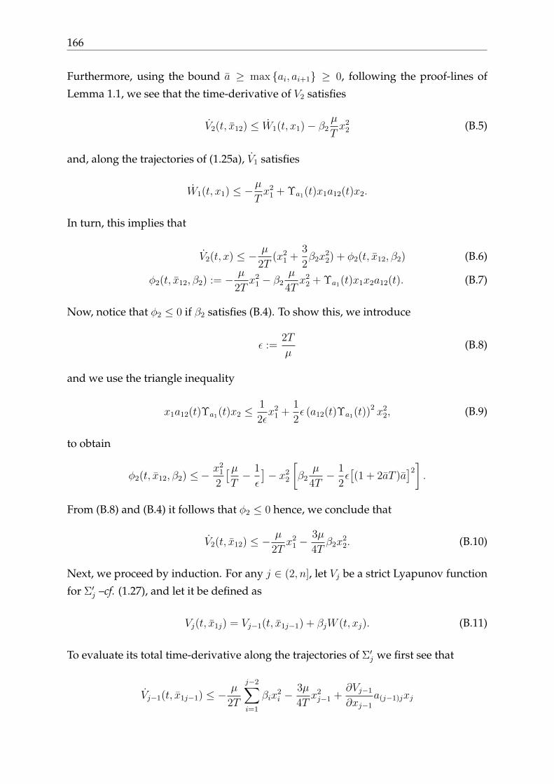
166
Furthermore, using the bound a ≥ max ai, ai+1 ≥ 0, following the proof-lines of
Lemma 1.1, we see that the time-derivative of V2 satisfies
V2(t, x12) ≤ W1(t, x1)− β2µ
Tx2
2 (B.5)
and, along the trajectories of (1.25a), V1 satisfies
W1(t, x1) ≤ −µTx2
1 + Υa1(t)x1a12(t)x2.
In turn, this implies that
V2(t, x) ≤ − µ
2T(x2
1 +3
2β2x
22) + φ2(t, x12, β2) (B.6)
φ2(t, x12, β2) := − µ
2Tx2
1 − β2µ
4Tx2
2 + Υa1(t)x1x2a12(t). (B.7)
Now, notice that φ2 ≤ 0 if β2 satisfies (B.4). To show this, we introduce
ε :=2T
µ(B.8)
and we use the triangle inequality
x1a12(t)Υa1(t)x2 ≤1
2εx2
1 +1
2ε (a12(t)Υa1(t))2 x2
2, (B.9)
to obtain
φ2(t, x12, β2) ≤− x21
2
[µT− 1
ε
]− x2
2
[β2
µ
4T− 1
2ε[(1 + 2aT )a
]2].
From (B.8) and (B.4) it follows that φ2 ≤ 0 hence, we conclude that
V2(t, x12) ≤ − µ
2Tx2
1 −3µ
4Tβ2x
22. (B.10)
Next, we proceed by induction. For any j ∈ (2, n], let Vj be a strict Lyapunov function
for Σ′j –cf. (1.27), and let it be defined as
Vj(t, x1j) = Vj−1(t, x1j−1) + βjW (t, xj). (B.11)
To evaluate its total time-derivative along the trajectories of Σ′j we first see that
Vj−1(t, x1j−1) ≤ − µ
2T
j−2∑i=1
βix2i −
3µ
4Tx2j−1 +
∂Vj−1
∂xj−1
a(j−1)jxj

Appendix B 167
and, in view of (B.11),∂Vj−1
∂xj−1
=[Υaj−1
(t)βj−1
]xj−1. (B.12)
Hence, it follows that
Vj(t, x1j) ≤ −µ
2T
j−1∑i=1
βix2i −
3µ
4Tx2j + φj(t, x1j, βj, βj−1)
where
φj(·) = − µ
4Tβj−1x
2j−1 + βj−1Υaj−1
(t)a(j−1)j(t)xjxj−1
− βjµ
4Tx2j . (B.13)
Now, in view of (B.7), the factor of βj−1Υaj−1(t)a(j−1)j(t)xjxj−1 is non-negative hence,
applying the triangle inequality to the last two terms on the right-hand side of (B.13),
we obtain that, for any ε > 0,
φj(·) ≤−µ
4Tβj−1x
2j−1 +
βj−1
2εx2j−1 + βj−1
ε
2
(Υaj−1
(t)a(j−1)j(t))2x2j
− βjµ
4Tx2j
which, in turn, using (1.5), we btain
φj(·) ≤ −[µ
4T− 1
2ε
]βj−1x
2j−1 +
[βj−1
ε
2((1 + 2T a) a)2 − βj
µ
4T
]x2j
for all ε 6= 0. To render non-positive the factors of x2j and x2
j−1 above, we choose
ε =2T
µ.
Then, the factor of x2j−1 equals to zero if (B.8) holds, while the factor of −x2
j is non-
negative if
βj ≥4T 2
µ2βj−1 [(1 + 2aT ) a]2
for all j ∈ (2, n] –cf. (1.29). It follows that φj ≤ 0 and, consequently,
Vj(t, x1j) ≤ −µ
2T
j−1∑i=1
x2i −
3µ
4Tx2j . (B.14)
The latter holds for any integer j ∈ [3, n] hence, together with (B.2) and (B.10), the
inequality (1.31) follows.

168
B.2 Proof of theorem 1.4
In view of (1.5), the boundedness of a and b, we have
V (t, x) ≥1
2[γ + Υa4b2(t)]x>Px− b2a3
∣∣∣∣∣P 1/2A
n∑i=1
βiΓiP1/2
∣∣∣∣∣x>PxV (t, x) ≤1
2
[γ + Υa4b2(t)
]x>Px+ b2a3
∣∣∣∣∣P 1/2An∑i=1
βiΓiP1/2
∣∣∣∣∣x>PxUsing the bound γ > γ2, the function V is positive definite and radially unbounded.
Indeed, there exist η1, η2 > 0 such that
η1|x|2 ≤ V (t, x) ≤ η2|x|2 (B.15)
for all t ≥ 0 and x ∈ Rn.
Next, we compute the total derivative of V along the trajectories of (1.63). We use
the persistency of excitation of the product ψ = a2b, (1.7) and (1.66), and we reorganise
some terms to obtain
V ≤ −γb2x>CC>x− µ
Tx>Px− a4b2x>
[βnPAΓnA
>P − P +n−1∑i=1
βiPAΓiA>P
]x
−ba2[[
2ba+ 3ba][PAx]> + ba2[PA2x]>
] n∑i=1
βiΓiPx
−b4a3[C>x]>n∑i=1
βiC>[AΓiP − ΓiPA
]x. (B.16)
To establish that V is negative definite we first note that, since the pair A,B is control-
lable by assumption, the matrix ΦcΦ>c where Φc corresponds to Kalman’s controllabil-
ity matrix Φc := [B AB · · · An−1B], is positive definite and satisfies ΦcΦ>c = AΓnA
>.
Hence, in view of the definition of βn we have −βnx>PAΓnA>Px+ x>Px ≤ 0. There-
fore, the sum of the first two terms in the second line of (B.16) is non-positive. Next,
note that the terms in the last line of (B.16) are bounded from above by
γ1b2|C>x|2 +
µPm2T b2
|x|2
where γ1 is defined in (1.68). Hence, using Γ1 = BB> and Γi = BB> + AΓi−1A for all
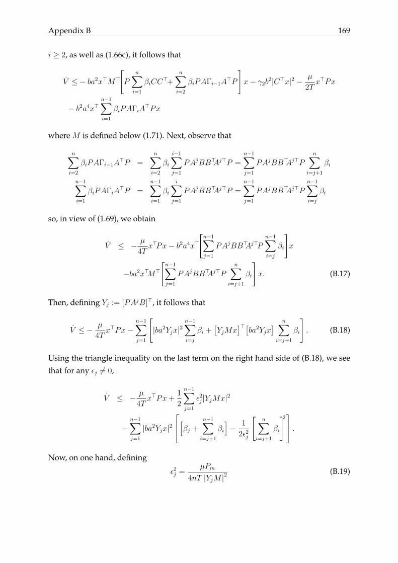
Appendix B 169
i ≥ 2, as well as (1.66c), it follows that
V ≤− ba2x>M>
[P
n∑i=1
βiCC>+
n∑i=2
βiPAΓi−1A>P
]x− γ2b
2|C>x|2 − µ
2Tx>Px
− b2a4x>n−1∑i=1
βiPAΓiA>Px
where M is defined below (1.71). Next, observe that
n∑i=2
βiPAΓi−1A>P =
n∑i=2
βi
i−1∑j=1
PAjBB>Aj>P =n−1∑j=1
PAjBB>Aj>P
n∑i=j+1
βi
n−1∑i=1
βiPAΓiA>P =
n−1∑i=1
βi
i∑j=1
PAjBB>Aj>P =n−1∑j=1
PAjBB>Aj>P
n−1∑i=j
βi
so, in view of (1.69), we obtain
V ≤ − µ
4Tx>Px− b2a4x>
[n−1∑j=1
PAjBB>Aj>Pn−1∑i=j
βi
]x
−ba2x>M>
[n−1∑j=1
PAjBB>Aj>Pn∑
i=j+1
βi
]x. (B.17)
Then, defining Yj := [PAjB]>, it follows that
V ≤− µ
4Tx>Px−
n−1∑j=1
[|ba2Yjx|2
n−1∑i=j
βi +[YjMx
]>[ba2Yjx
] n∑i=j+1
βi
]. (B.18)
Using the triangle inequality on the last term on the right hand side of (B.18), we see
that for any εj 6= 0,
V ≤ − µ
4Tx>Px+
1
2
n−1∑j=1
ε2j |YjMx|2
−n−1∑j=1
|ba2Yjx|2[βj +
n−1∑i=j+1
βi
]− 1
2ε2j
[n∑
i=j+1
βi
]2 .Now, on one hand, defining
ε2j =µPm
4nT |YjM |2(B.19)
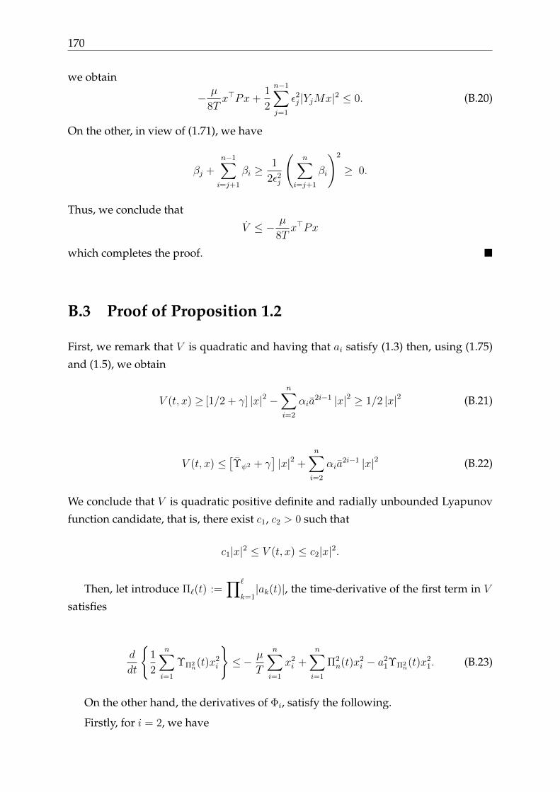
170
we obtain
− µ
8Tx>Px+
1
2
n−1∑j=1
ε2j |YjMx|2 ≤ 0. (B.20)
On the other, in view of (1.71), we have
βj +n−1∑i=j+1
βi ≥1
2ε2j
(n∑
i=j+1
βi
)2
≥ 0.
Thus, we conclude that
V ≤ − µ
8Tx>Px
which completes the proof.
B.3 Proof of Proposition 1.2
First, we remark that V is quadratic and having that ai satisfy (1.3) then, using (1.75)
and (1.5), we obtain
V (t, x) ≥ [1/2 + γ] |x|2 −n∑i=2
αia2i−1 |x|2 ≥ 1/2 |x|2 (B.21)
V (t, x) ≤[Υψ2 + γ
]|x|2 +
n∑i=2
αia2i−1 |x|2 (B.22)
We conclude that V is quadratic positive definite and radially unbounded Lyapunov
function candidate, that is, there exist c1, c2 > 0 such that
c1|x|2 ≤ V (t, x) ≤ c2|x|2.
Then, let introduce Π`(t) :=∏`
k=1|ak(t)|, the time-derivative of the first term in V
satisfies
d
dt
1
2
n∑i=1
ΥΠ2n(t)x2
i
≤− µ
T
n∑i=1
x2i +
n∑i=1
Π2n(t)x2
i − a21ΥΠ2
n(t)x2
1. (B.23)
On the other hand, the derivatives of Φi, satisfy the following.
Firstly, for i = 2, we have
d
dt
a2
1Φ2
≤− a2
1a22x
22 + a2
1a3 |x1x2|+ a2
1a2 |x1x3|+ 4 |a1| a2 |x1x2|+ a2
1a2x2
1 (B.24)
and, similarly, for each i ∈ [3, n− 1], we obtain
d
dt
a2
1Φi
≤2i
i−1∑j=1
Πj a(2i−1−j) |xjxj+1|+
i−1∑j=1
Π2j(t)a
2(i−j) |xjxj+2|
+ a1(t)2a2(i−1)x21 − Π2
i (t)x2i + a2
1a2i−1 |x1x2| (B.25)
while, for i = n,
d
dt
a2
1Φn
≤− Π2
n(t)x2n + a1(t)2a2i−1 |x1x2|+
n−2∑j=1
Π2j(t)a
2(n−j) |xjxj+2|
+ a1(t)2a2(n−1)x21 + 2n
n−1∑j=1
Πj(t)a(2n−1−j) |xjxj+1|. (B.26)
Thus, putting together (B.23) up to (B.26) we get
V (t, x) ≤− µ
2T|x|2 −
n∑i=2
[αi − an−i]Π2i (t)x
2i −
µ
4T|x|2 +
n∑i=3
i−1∑j=2
Π2j(t)
[a2(i−j)αi |xjxj+2|
]+
n∑i=3
i−1∑j=2
Πj(t)[αi2ia
(2i−1−j) |xjxj+1|]
+ φ1(t, x)
where we defined
φ1(t, x) :=n∑i=2
αi[a1(t)a2i−1 |x1x2|+ a2
1a2(i−1)x2
1 + a21a
2(i−1) |x1x3|
+2i |a1| a2(i−1) |x1x2|]− γa1(t)2x2
1 −µ
4T|x|2. (B.27)
Now, notice that all positive terms above are (bounded by) cross products of |x2|and |x3|with |a1x1| hence, they may be upper-bounded by
λ[a1x1]2 +1
λ[ε2x
22 + ε3x
23]
for appropriate values of ε2, ε3 and λ. It follows that for sufficiently small λ and choos-
172
ing γ sufficiently large, as in (1.75), we have φ1 ≤ 0. Therefore,
V (t, x) ≤− µ
2T|x|2 + φ2(t, x)
where we defined
φ2(t, x) :=−n∑i=2
[αi − an−i
]Πi(t)
2x2i −
µ
4T|x|2
+n∑i=3
i−1∑j=2
Πj(t)[Πj(t)a
2(i−j)αi |xjxj+2|+ 2ia(2i−1−j) |xjxj+1|].
It is left to prove that φ2 ≤ 0. To that end, we start by changing the order of sum-
mation. Hence,
φ2(t, x) =−n∑i=2
[αi − an−i
]Πi(t)
2x2i −
µ
4T|x|2 +
n−2∑i=2
Πi(t)2 |xixi+2|
n∑j=i+1
a2(j−i)αj
+n−1∑i=2
Πi(t) |xixi+1|n∑
j=i+1
αj2ia(2j−1−i)
which satisfies
φ2(t, x) ≤ − µ
4nTx2n +
n−2∑i=2
[−[αi − an−i
]Π2ix
2i + Π2
i
n∑j=i+1
a2(j−i)αj −µ
4nT
[x2i+1 + x2
i+2
]+Π2
i
n∑j=i+1
a2(j−i)αj |xixi+2|+n∑
j=i+1
αj2ia(2j−1−i)Πi |xixi+1|
]−[αn−1 − a
]Π2n−1x
2n−1
+ [αn2(n− 1)an] Πn−1|xn−1xn|
Now, as for φ1 in (B.27), we see that the cross terms in the first summation above
may be upper-bounded using the triangle inequality. That is, we use
2|xixi+2| ≤ εix2i +
1
εix2i+2, 2|xixi+1| ≤ δix
2i +
1
δix2i+1,
which holds for any εi, δi > 0. In particular, setting
εi =2nT
µ
n∑j=i+1
a2jαj, δi =2nT
µ
n∑j=i+1
[αj2ia
(2j−1−i)]

Appendix B 173
we see that choosing αn = 1 and αn−1 according to (1.73), while
αi = an−i +µ
4nTδ2i +
εi2
[n∑
j=i+1
αj a2(j−i)
],
φ2 is non-positive for all t and x –cf. (1.74).
B.4 Proof complement for Proposition 2.1
First, we show that the total derivative of V2 along the trajectories of e = Avr(t, e)e is
negative definite. Firstly, since ρ1 is a polynomial that maps R≥0 → R≥0 and V1 satisfies
(2.26),d
dtρ1(V1)V1 ≤ −ρ1(V1)
[kxe
2x + kθe
2θ
]. (B.28)
Next, we use (2.31), as well as |e| ≥ |ey| and Υϕ > 0, to obtain
d
dt
[Υv2
r+ Υω2
r]V1
≤− 2
T
[∫ t+T
t
[ωr(s)
2 + vr(s)2]ds
]V1
+ [ω2r + v2
r ][e2x +
1
kye2θ + e2
y] (B.29)
Then, using (2.36) and (2.38), we obtain
− d
dtωrexey = −ωrexey − ωr
[− kxexey + ωre
2y + kθeθe
2y
+ kyvre3y − ωre2
x − kθeθe2x − kyvreye2
x + vreθex]. (B.30)
Now, for the cross-terms we use the inequalities 2exey ≤ εe2x + (1/ε)e2
y and 2eθe2y ≤
εV1e2θ + (1/ε)e2
y, which hold for any ε > 0, and we regroup some terms to obtain
− d
dtωrexey ≤ −ωr
[− kxexey + ωre
2y + kθeθe
2y + kyvre
3y
]− ωr
[− ωre2
x − kθeθe2x − kyvreye2
x + vreθex
]− ωrexey
≤− ω2re
2y + ωrkx
(ε
2e2x +
1
2εe2y
)+ ωrkθ
(εV1e
2θ +
1
2εe2y
)+ ωrvrkye
3y + ω2
re2x + ωr
kθ2
(e2θ + 2V1e
2x
)+ ωrkyvr
(1
2εe2y +
ε
2V1e
2x
)+ωrvr
2
(e2θ + e2
x
)+ ¯ωr
(ε
2e2x +
1
2εe2y
)
174
≤− ω2re
2y + ωrvrkye
3y +
1
2ε
[(kx + kθ)ωr + ωrkyvr + ¯ωr
]e2y
+[ωrkx
ε
2+ ω2
r + ωrkyvrε
2V1 + ¯ωr
ε
2+ωrvr
2+ ωrkθV1
]e2x
+[ωrkθεV1 + ωrkθ +
ωrvr2
]e2θ (B.31)
≤− ω2re
2y +
ε
2v2rV1e
2y + ρ5(V1)e2
x + ρ6(V1)e2θ
+1
2ε
[ω2rk
2y + (kx + kθ)ωr + ωrkyvr + ¯ωr
]e2y (B.32)
where ρ5 and ρ6 are first-order polynomials of V1 defined as
ρ5(V1) =ωr2
[(εkyvr + 2kθ
)V1 +
(kx +
¯ωrωr
)ε+ 2ωr + vr
]ρ6(V1) = ωr
[kθ(εV1 + 1) +
vr2
].
Next, we have
d
dtvrρ2(V1)eθey = −ρ2(V1)v2
re2y − vrρ2(V1)
[kθeθey + ωrexeθ
+ kθe2θex + kyvreyexeθ + vre
2θ
]+ ρ2(V1)vreθey
− vr∂ρ2
∂V1
eθey[kxe
2x + kθe
2θ
]. (B.33)
Hence, using again the triangle inequality to bound the cross-terms and regrouping
them, we obtain
d
dtvrρ2(V1)eθey ≤ − kyv2
rρ2e2y − ρ2kθvreθey − ρ2vr
[ωrexeθ + kθe
2θex + kyvreyexeθ
]+ ρ2v
2re
2θ + ρ2vreθey − vr
∂ρ2(V1)
∂V1
eθey(kxe
2x + kθe
2θ
)
Appendix B 175
≤− kyv2rρ2e
2y + kθvr
(ε
2ρ2
2e2θ +
1
2εe2y
)+ ρ2vr
ωr2
(e2x + e2
θ
)+ ρ2vr
kθ2
(e2θ + V1e
2x
)+ ρ2kyv
2r
(V1e
2x +
e2θ
2
)+ v2
rρ2e2θ+
¯vr
(ε
2ρ2
2e2θ +
1
2εe2y
)+ vr
∣∣∣∣∂ρ2(V1)
∂V1
∣∣∣∣maxky, 1V1
(kxe
2x + kθe
2θ
)
≤− kyv2rρ2e
2y +
1
2ε(kθvr + ¯vr) e
2y +
[ρ2vr
ωr2
+ kθV1ρ2vr
+ρ2kyv2rV1 + vr
∣∣∣∣∂ρ2(V1)
∂V1
∣∣∣∣maxky, 1V1kx
]e2x
+
[kθvr
ε
2ρ2
2 + ρ2vrωr2
+ ρ2vrkθ2
+ ρ2ky2v2r + v2
rρ2
+¯vrε
2ρ2
2 + vr
∣∣∣∣∂ρ2(V1)
∂V1
∣∣∣∣maxky, 1V1kθ
]e2θ
≤− kyv2rρ2e
2y + ρ7(V1)e2
x + ρ8(V1)e2θ +
1
2ε(kθvr + ¯vr) e
2y (B.34)
where ρ7 and ρ8 are second-order polynomials of V1 satisfying
ρ7(V1) ≥ ρ2vr[ ωr
2+ (kθ + kyvr)V1
]+ maxky, 1kxvrV1
∣∣∣∣∂ρ2
∂V1
∣∣∣∣ρ8(V1) ≥ vrρ2(V1)
2
[ωr + kθ(ερ2(V1) + 1) + (ky + 2)vr
]¯vrε
2ρ2(V1)2 + vr
∣∣∣∣∂ρ2
∂V1
∣∣∣∣maxky, 1kθV1.
Now we put all the previous bounds together. Using (2.21) in (B.29), we obtain, in
view of (B.31) and (B.34),
∂V2
∂t+∂V2
∂eAvr(t, e)e ≤ −
2µ
TV1(e)−
[kyρ2(V1)− 1− ε
2V1
]v2re
2y
+1
2ε
[ωr[ωrk
2y + kx + kθ + kyvr
]+ ¯ωr + kθvr + ¯vr
]e2y
− e2x
[kxρ1 − ρ7 − ρ5 − v2
r − ω2r
]− e2
θ
[kθρ1 − ρ8 − ρ6 −
1
ky
(v2r + ω2
r
)]. (B.35)

176
Hence, defining
ε :=T
µ
[ωr[ωrk
2y + kx + kθ + kyvr
]+ ¯ωr + kθvr + ¯vr
]ρ1(V1) := 1 +
1
minkx, kθ
[ρ5 + ρ6 + ρ7 + ρ8 +
[1 +
1
ky
][ω2r + v2
r
] ].
ρ2(V1) :=1
ky
[1 +
ε
2V1
]we obtain
∂V2
∂t+∂V2
∂eAvr(t, e)e ≤ −
µ
TV1(e)− kxe2
x − kθe2θ. (B.36)
That is, V2 is a strong Lyapunov function for the nominal dynamics e = Avr(t, e)e.
Next, we evaluate the total derivative of V along the trajectories of (2.35) (i.e., in-
cluding the output injection term). From (B.36) we obtain
V3(t, e) ≤ ∂V2
∂t+∂V2
∂eAvr(t, e)e+W (t, e) (B.37)
W (t, e) := −kθρ4(V1)e2θ + vr[φ(eθ)− 1]
∂V2
∂eB(ey)e (B.38)
for which we used (2.26), as well as the positivity of ρ4(V1) and of ∂ρ4/∂V1, to obtain
d
dtV1ρ4(V1) = V1ρ4(V1) + V1
∂ρ4
∂V1
V1 ≤ −kθρ4(V1)e2θ.
We show that W (t, e), defined in (B.38), is non-positive. To that end, note that
[φ(eθ)− 1] ≤ e2θ (B.39)
and, in view of the structure of B, we have
∂V1
∂eB(e)e = 0
hence,∂V2
∂e= vrρ2(V1)[ey 0 eθ]− ωr[0 ey ex]
and, moreover,
∣∣ [ey 0 eθ]B(e)e
∣∣ =∣∣− kye2
y + e2θ − kyeyexeθ
∣∣ ≤ ∣∣e2θ −
ky2e2y +
ky2e2xe
2θ
∣∣≤ 2kyV1 + 2k2
yV2
1∣∣ [0 ey ex]B(e)e ∣∣ =∣∣kye3
y + eθex − kyeye2x
∣∣ ≤ 2kyV2
1 + maxky, 1V1.
Appendix B 177
Thus, W (t, e) ≤ 0 if
ρ4(V1) ≥ 2vr maxky, 1kθ
[ [kyρ2vr + ωr
]V 2
1 +[ρ2vr + ωr
]V1
]and (2.34) follows from (B.36) and (B.37).
B.5 Proof of Proposition 2.2
Consider the function W : R≥0 × R3 → R≥0 defined by
W (t, e) := ln[1 + V (t, e)
](B.40)
where V : R≥0 → R3 → R≥0 is the continuously differentiable function defined in
(2.28).
The total derivative of W along the trajectories of (2.47) yields
W (t, e) ≤ V (t, e)
1 + V (t, e)
which, in virtue of (2.29) implies that
W (t, e) ≤ −α(|e|) +∂V
∂e
B(e)η
1 + V (t, e)(B.41)
where
α(|e|) =µ
2T
V1(e)
1 + V (t, e).
To establish the statement of the proposition we show that the second term on the
right hand side of (B.41) is bounded from above by γ|η| with γ > 0. For the sake of
argument, remark that V (t, e) = V(t, e, V1) where
V(t, e, V1) := P[3](t, V1)V1 − ωr(t)exey + vr(t)P[1](t, V1)eθey
and, in addition, note that there exists a fourth-order polynomial P4(V1) such that
V(t, e, V1) ≥ P4(V1), ∀ (t, e, V1) ∈ R≥0 × R3 × R≥0. (B.42)
Furthermore,∂V
∂e=
∂V∂V1
∂V1
∂e+∂V∂e

178
Therefore
∂V
∂e
[B(e)η
]=∂V∂V1
∂V1
∂eB(e)η +
∂V∂e
[B(e)η
]Now, since P[3] is a polynomial of 3rd order, we have
∂V∂V1
= P ′[3](V1) + vr(t)∂P[1]
∂V1
eθey
where P ′[3] : R≥0 → R≥0 is the polynomial function of 3rd order defined as
P ′[3](V1) :=∂P[3]
∂V1
V1 + P[3](V1).
Then, since P[1] is a polynomial of 1st order and eθey ≤ V1(e), there exists c > 0 such
that ∣∣∣∣ ∂V∂V1
∣∣∣∣ ≤ P ′[3](V1) + cvrV1.
Furthermore, B(e) is linear in e therefore, there exists c > 0 such that∣∣∣∣∂V1
∂eB(e)η
∣∣∣∣ ≤ cV1|η|
and, on the other hand,
∂V∂e
>=
vr(t)P[1](t, V1)ey
−ωr(t)eyvr(t)P[1](t, V1)eθ − ωr(t)ex
(B.43)
Putting all these bounds together, we conclude that there exists a polynomial of fourth
order P ′4(V1) such that ∣∣∣∣∂V∂e [B(e)η]∣∣∣∣ ≤ P ′4(V1)|η|.
and, therefore,
W (t, e) ≤ −α(|e|) + c|η|
where
c := lim supV1≥0
P ′4(V1)
1 + P4(V1)
and the claim follows.

Appendix B 179
B.6 Proof of Lemma 2.1
First, we remark that V2, hence V , is positive definite and radially unbounded. This
follows since γ1(V1)V1 > (φ/2)V 21 and
−φ(t)V1(e)exey +φ
2V1(e)2 =
V1
2
[ex
ey
]> [φ φ
φ φ
][ex
ey
]≥ 0.
Next, we proceed now to compute the total derivative of V . By the fundamental
theorem of calculus, we have
Υφ(s)2(t) = − 1
T
∫ t+T
t
φ(s)2ds+ φ(t)2.
Now, let µ, T > 0 be generated by the assumption that φ is persistently exciting. Then,
Υφ(s)2(t) ≤ −µT
+ φ(t)2.
Therefore, the time-derivative of V2 along the trajectories of the system[ex
ey
]=
[−kx φ[e2
y + e2x]
−φ[e2y + e2
x] 0
][ex
ey
](B.44)
satisfies
V2 ≤ −µTV 3
1 + φ2V 31 − φ2e2
yV2
1 + kxφexeyV1
−2kxγ3(V1)e2x − φexeyV1 + 2φeykxe
3x + φ2V 2
1 e2x
≤ − µ
2TV 3
1 −µ
2Te6y + φ2
(e4x + 3e2
xe2y + 3e4
y
)e2x
+φ2e6y − φ2e2
yV2
1 + kxφexey[e2x + e2
y]− 2kxγ3(V1)e2x
−φexeyV1 + 2φexeykxe2x + φ2V 2
1 e2x

180
Now, we use V1 = [e2x + e2
y] and the inequalities
φ2(e4x + 3e2
xe2y + 3e4
y
)e2x ≤ 3φ2V 2
1 e2x,
φ2e6y − φ2e2
yV2
1 ≤ 0,
3φexeykxe2x ≤
3
2V1φkxe
2x,
φexeykxe2y ≤
φ
2
[1εe6y + εk2
xe2x
],
−φexey[e2y + e2
x] ≤φ
2
[1εe6y + εe2
x + e2xV1
]to obtain
V2 ≤ − µ
2TV 3
1 −[µ
2T− φ
ε
]e6y
−[2kxγ3(V1)− 4φ2V 2
1 −3
2φkxV1 −
εφ
2[k2x + 1]− φ
2V1
]e2x
so, setting ε = 4T φµ
and γ3(V1) as in (2.74), we obtain
V2 ≤−µ
2TV 3
1 −µ
4Te6y. (B.45)
Next, we compute the total derivative of V (t, e) (recall that e := [ex ey ez]>) in (2.69)
along the trajectories of (2.66). Using (B.45), we obtain
V3 ≤ −2γ1(V1)kxe2x −
µ
2TV 3
1 −µ
4Te6y
+∂V2
∂V1
∂V1
∂[ex ey]>
[0 kθ
−kθ 0
][ex
ey
]ez
−∂(φV1exey)
∂[ex ey]>
[0 kθ
−kθ 0
][ex
ey
]ez
+2γ2(V1)ez[−kθez − 2φkxe2x].
However,∂V1
∂[ex ey]>
[0 kθ
−kθ 0
][ex
ey
]= 0
hence,
V3 ≤ − µ
4Te6y − kθφez[e4
y − e4x]− 2kθγ2(V1)e2
z
−4φ(t)kxγ2(V1)eze2x − 2γ1(V1)kxe
2x −
µ
2TV 3
1 .

Appendix B 181
Now, for any ε1, ε2 > 0 we have
−kθφeze4y ≤
1
2ε1φkθe
2ze
2y +
ε12φkθe
6y
kθφeze4x ≤
1
2ε1φkθe
2zV1 +
ε12φkθe
2xV
21
−4φ(t)kxγ2(V1)eze2x ≤
2φ
ε2kxγ2(V1)e2
z + 2ε2φkxγ2(V1)V1e2x,
therefore
V3(t, e) ≤ − µ
4TV 3
1 −[ µ
4T− ε1
2φkθ
]e6y
−[2γ1(V1)kx −
ε12φkθV
21 − 2ε2kxφγ2(V1)V1
]e2x
−[2kθγ2(V1)−
[kθε1V1 +
2
ε2kxγ2(V1)
]φ]e2z.
So, setting
ε1 :=µ
4T φkθ, ε2 :=
4kxφ
kθ
and using (2.72)–(2.74), (2.75) follows.
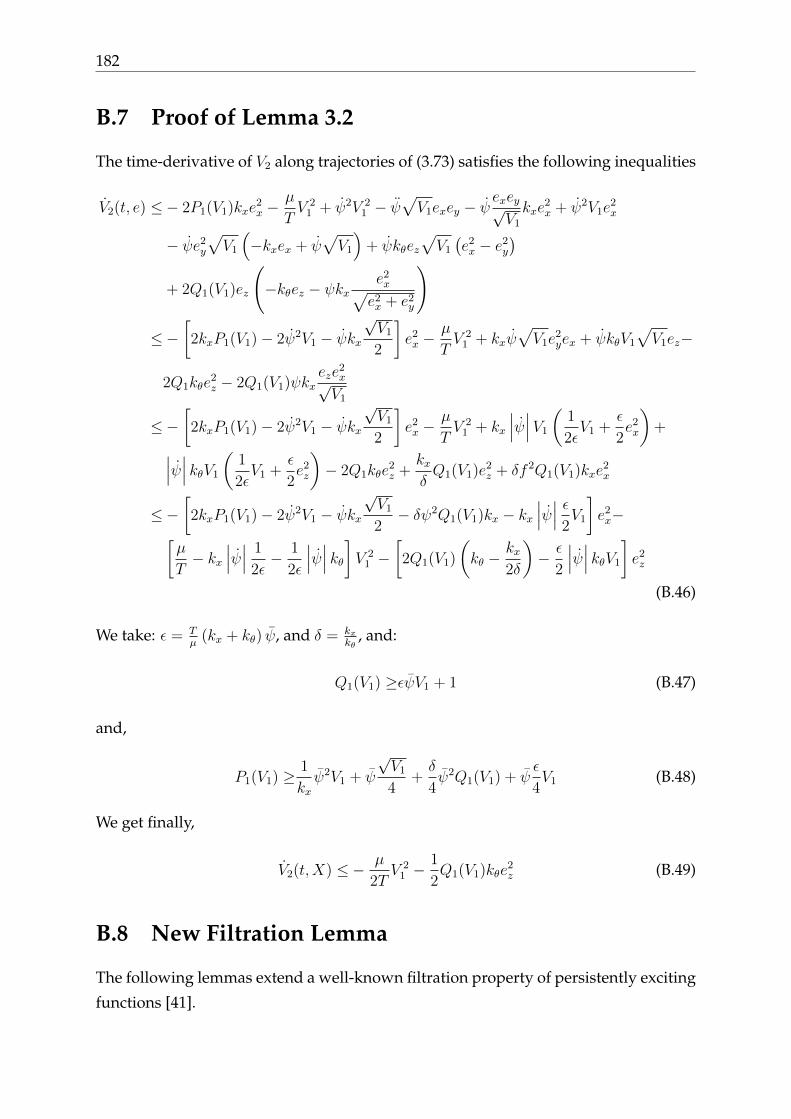
182
B.7 Proof of Lemma 3.2
The time-derivative of V2 along trajectories of (3.73) satisfies the following inequalities
V2(t, e) ≤− 2P1(V1)kxe2x −
µ
TV 2
1 + ψ2V 21 − ψ
√V1exey − ψ
exey√V1
kxe2x + ψ2V1e
2x
− ψe2y
√V1
(−kxex + ψ
√V1
)+ ψkθez
√V1
(e2x − e2
y
)+ 2Q1(V1)ez
(−kθez − ψkx
e2x√
e2x + e2
y
)
≤−[2kxP1(V1)− 2ψ2V1 − ψkx
√V1
2
]e2x −
µ
TV 2
1 + kxψ√V1e
2yex + ψkθV1
√V1ez−
2Q1kθe2z − 2Q1(V1)ψkx
eze2x√V1
≤−[2kxP1(V1)− 2ψ2V1 − ψkx
√V1
2
]e2x −
µ
TV 2
1 + kx
∣∣∣ψ∣∣∣V1
(1
2εV1 +
ε
2e2x
)+∣∣∣ψ∣∣∣ kθV1
(1
2εV1 +
ε
2e2z
)− 2Q1kθe
2z +
kxδQ1(V1)e2
z + δf 2Q1(V1)kxe2x
≤−[2kxP1(V1)− 2ψ2V1 − ψkx
√V1
2− δψ2Q1(V1)kx − kx
∣∣∣ψ∣∣∣ ε2V1
]e2x−[
µ
T− kx
∣∣∣ψ∣∣∣ 1
2ε− 1
2ε
∣∣∣ψ∣∣∣ kθ]V 21 −
[2Q1(V1)
(kθ −
kx2δ
)− ε
2
∣∣∣ψ∣∣∣ kθV1
]e2z
(B.46)
We take: ε = Tµ
(kx + kθ) ψ, and δ = kxkθ
, and:
Q1(V1) ≥εψV1 + 1 (B.47)
and,
P1(V1) ≥ 1
kxψ2V1 + ψ
√V1
4+δ
4ψ2Q1(V1) + ψ
ε
4V1 (B.48)
We get finally,
V2(t,X) ≤− µ
2TV 2
1 −1
2Q1(V1)kθe
2z (B.49)
B.8 New Filtration Lemma
The following lemmas extend a well-known filtration property of persistently exciting
functions [41].

Appendix B 183
Lemma B.1. Consider the two scalar second order systems:
f + k1f + k2f = p(t) (B.50)
and
q(3) + k1q + k2q = p(t) (B.51)
where k1, k2 > 0 and p(t) is a time-varying input such that p(t) is PE with excitation
parameters−(T, µ) and there exists bp > 0 such that maxp, p, p, p(3)
≤ bp. Then f(t)
and q(t) are both PE with excitation parameters−(Tf , µf ) and−(Tq, µq) respectively, given by
Tf = kfT ,
µf =
(2(1 + k−1
2 )bprf)2
b2p
(1 + k1k
−12 + k−1
2
)2Tf, (B.52)
and kf =
[4(1+k−1
2 )bprfµk−1
2
]+ 1, Tq = kqT ,
µq =(2bprq(2 + k2))2
b2p(1 + k1 + k2)2Tq
, (B.53)
and kq =[
4µbprq(2 + k2)
]+ 1.
Where
r2f =
(a+ 1)f(0)2 + 4(ak2 + 1)(f(0)2 + k−1
2 bp2)
+ bbp2
c
min 1, k2, (B.54)
r2q =
2(a+ 1)q(0)2 + 4(ak2 + 1)
(q(0)2 + k−2
2 b2p
)+
bb2pc
+ k−22 bp
min 1, k2,
a = 2k−11 + k1k
−12 + k−1
2 + 1, b := 4k−12 + 1
ak1k22
and c := 14
minak1,k2a+2+ak2
.
Furthermore,
maxf, f , f , f (3)
≤ bf ,
maxq, q, q, q(3)
≤ bq,
with:
bf =[2 + k1 + k2 + k2
1 + k1k2 + k2
]rf + [k1 + k−2 + 2]bp. (B.55)
bq =
(2 + k1 + k2 +
2
k2
(k1 + 1)
)rq +
(1 +
2
k2
)bp + |q(0)| . (B.56)
Proof. 1)- Consider the following linear change of coordinates for the first differential

184
equation (B.50): x = f − k−12 p(t), y = f . Then x = y − k−1
2 p(t) and y = −k2y − k1x.
First, note that the overall trajectories are bounded, i.e., there exists rf > 0 that is a
function of (x(0), y(0), bp), such that |(x, y)| ≤ rf , ∀t ≥ 0. Consider now the following
time-derivative
d
dt
[−px− k−1
2 py]
=[−p+ k1k−12 p− k−1
2 p(3)]y + k−12 p2
≥− bp[1 + k1k
−12 + k−1
2
]|y|+ k−1
2 p2,
then
bp[1 + k1k
−12 + k−1
2
] ∫ t+kfT
t
|y(s)|ds ≥∫ t+kfT
t
d
ds
[p(s)x(s) + k−1
2 p(s)y(s)]ds+
k−12
∫ t+kfT
t
p(s)2ds ≥ −2(1 + k−1
2
)bprf + k−1
2 kfµ
where kf is a positive integer and, to obtain the last inequality, we used the fact that
trajectories are bounded and that p is PE with parameters (T, µ). Invoking the Cauchy-
Schwartz inequality on∫ t+kfTt
|y(s)|ds, we obtain
b2p
(1 + k1k
−12 + k−1
2
)2kfT
∫ t+kfT
t
y(s)2ds ≥(k−1
2 kfµ− 2(1 + k−1
2
)bp)2
Finally, we get ∫ t+kfT
t
y(s)2ds ≥(k−1
2 kfµ− 2(1 + k−1
2
)bprf
)2
b2p
(1 +K1k
−12 + k−1
2
)2kfT
(B.57)
Taking kf =
[4(1+k−1
2 )bprfµk−1
2
]+ 1, we find Tf = kfT and µf =
(2(1+k−12 )bprf)
2
b2p(1+k1k−12 +k−1
2 )2Tf
, such that
t+Tf∫t
y(s)2ds ≥ µf . 2)- Consider the second equation case using the notation (x, y) =
(q, q). First, note that the overall trajectories are bounded, i.e., there exists rq > 0 that is
a function of (x(0), y(0), bp), such that ‖(x, y)‖ ≤ rq, ∀t ≥ 0. Consider now the following
time-derivative
d
dt[py − (p− k2p)x] =− [pk1 + p(3) − k2p]x+ p2
≥− bp [k1 + 1 + k2] |x|+ p2,
Appendix B 185
then
bp [k1 + 1 + k2]
∫ t+kqT
t
|x(s)|ds ≥∫ t+kqT
t
d
ds[py − (p− k2p)x]ds+∫ t+kqT
t
p(s)2ds ≥ −2 (2 + k2) bpr + kqµ
where kq is a positive integer and, to obtain the last inequality, we used the fact that
trajectories are bounded and that p is PE with parameters (T, µ). Invoking the Cauchy-
Schwartz inequality on∫ t+kqTt
|x(s)|ds, we obtain
b2p (k1 + k2 + 1)2 kqT
∫ t+kqT
t
x(s)2ds ≥
(kqµ− 2 (2 + k2) bprq)2
Finally, we get ∫ t+kT
t
x(s)2ds ≥ (2bprq(2 + k2))2
b2p(1 + k1 + k2)2Tq
(B.58)
Taking kq =[
4µbprq(2 + k2)
]+ 1, we find Tq = kqT and µq = (2bprq(2+k2))2
b2p(1+k1+k2)2Tq, such that
t+Tq∫t
x(s)2ds ≥ µq. In order to have an explicit estimation of (Tf , µf ) and (Tq, µq) it only
remains to estimate the upper bound of the trajectories rf and rq. For, let consider
the first deferential equation (B.50) and let us define the Lyapunov function candidate
V (x, y) = a (y2 + k2x2) + xy with x = f − k−2 p(t), y = f and a = 2k−1
1 + k1k−12 + k−1
2 + 1.
V (x, y) verifies the following bounds
min 1, k2(y2 + x2) ≤ V (x, y) ≤
max a+ 1, ak2 + 1 (x2 + y2). (B.59)
V , along the trajectories of the system, satisfies
V (·) ≤− ak1y2 + y2 − k1yx− k2x
2 + 2px+ k−12 yp
≤− a
4k1y
2 − 1
4k2x
2 +
[4k−1
2 +1
ak1k22
]p2
≤− cV + bb2p
where c := 14
minak1,k2a+2+ak2
and b := 4k−12 + 1
ak1k22.
Since x2 + y2 ≤ 1min1,k2V , we can calculate the upper bound of the trajectories as

186
‖(x, y)‖2 ≤ 1
min 1, k2max
V (0),
bb2p
c
≤
(a+ 1)f(0)2 + 4(ak2 + 1)(f(0)2 + k−2
2 b2p
)+
bb2pc
min 1, k2= r2
f . (B.60)
To deduce the bound rq using rf we observe that the differential equations (B.50)
is equivalent to (B.51) if we replace f by q and f by q, also under the assumption
maxp, p, p, p(3)
≤ bp we obtain,
(q − k2p)2 + q2 ≤
(a+ 1)q(0)2 + 4(ak2 + 1)(q(0)2 + k−2
2 b2p
)+
bb2pc
min 1, k2. (B.61)
which implies,
q2 + q2 ≤
2(a+ 1)q(0)2 + 4(ak2 + 1)
(q(0)2 + k−2
2 b2p
)+
bb2pc
+ k−22 bp
min 1, k2= rq. (B.62)
Finally, from the system dynamics, (B.60) and (B.62), we can find that f ≤ rf + k−2 bp,
f ≤ rf , f ≤ (k1 + k2)rf + bp and f (3) ≤ (k21 + k1k2 + k2)rf + (k1 + 1)bp so (B.55) follows.
Also, q ≤ rq, q ≤ rq, q(3) ≤ k1rq + k2rq + bp and q ≤ 2k2bp + 2
k2(k1 + 1)rq + |q(0)| so (B.56)
follows. This concludes the proof.
B.9 Proof of theorem 4.1
First, we remark that W (·) and Z(·) are positive definite radially unbounded and sat-
isfy
W (·) ≥γ(V )V
W (·) ≤γ(V )V + V κT (e, s)Υf2(t)κ(e, s) + c1bf2λN(L)V 2+
2 [λN(L) + |Kpt|]α(V )V
Z(·) ≥min 1, λm(Kpθ)[eTθ eθ + eTωeω
]Z(·) ≤max 1 + c2, c2λM(Kpθ) + 1
[eTθ eθ + eTωeω
]. (B.63)
Appendix B 187
Next, we study the time derivative of each component in the Lyapunov function Γ(·)along the trajectories of the closed-loop system (4.25), that is,
d
dt(γ(V )V ) ≤− γ(V )vTKdtK
−ptv, (B.64)
d
dt(ρ2(V )V ) ≤− ρ2(V )vTKdtK
−ptv, (B.65)
d
dt
(V κT Υf2(t)κ
)≤ −V κT 1
T
∫ t+T
t
f 2(s)dsκ+
V κT f 2(t)κ+ 2V κT Υf2
[eΦTL2Φv + sΦ⊥TL2Φv
]. (B.66)
Since f(t) is persistently exciting, with parameters−(µ, T ), then the following inequal-
ities holds
d
dt
(V κT Υf2(t)κ
)≤ −µ
TV κTκ+ V κT f 2(t)κ+
2V κT Υf2
[eΦTL2Φv + sΦ⊥TL2Φv
]≤− µ
TV κTκ+ V κT f 2(t)κ+ 2V eT κΥf2ΦTL2Φv+
2V sT κΥf2Φ⊥TL2Φv (B.67)
where we used the facts that
κT Υf2 eΦTL2Φv = eT κΥf2ΦTL2Φv
and
κT Υf2 sΦ⊥TL2Φv = sT κΥf2Φ⊥TL2Φv.

188
Moreover, we have
d
dt
(V κT Υf2(t)κ
)≤ −µ
TV κTκ+ V κT f 2(t)κ+
V
[1
εeT κe+ εvTΦTL2ΦΥ2
f2κΦTL2Φv
]+
V
[1
εsT κs+ εvTΦ⊥TL2ΦΥ2
f2κΦ⊥TL2Φv
]≤− µ
TV κTκ+ V κT f 2(t)κ+ V
2
εκTκ+
V εvTΦTL2ΦΥ2f2κΦTL2Φv+
V εvTΦ⊥TL2ΦΥ2f2κΦ⊥TL2Φv
≤−[µ
T− 2
ε
]V κTκ+ V κT f 2(t)κ+
V 2ελN(L)(∣∣Υf2ΦTL2Φ
∣∣2∞ +
∣∣Υf2Φ⊥TL2Φ∣∣2∞
)×∣∣K−dtKpt
∣∣ vTKdtK−ptv (B.68)
where the following inequality
vTΦTL2ΦΥ2f2κΦTL2Φv ≤ λN(L)V
∣∣Υf2ΦTL2Φ∣∣2∞
∣∣K−dtKpt
∣∣×vTKdtK
−ptv, (B.69)
vTΦ⊥TL2ΦΥ2f2κΦ⊥TL2Φv ≤ λN(L)V
∣∣Υf2Φ⊥TL2Φ∣∣2∞×∣∣K−dtKpt
∣∣ vTKdtK−ptv, (B.70)
and
sT κs ≤ 2κTκ
are used in order to obtain
d
dt
(V κT Υf2(t)κ
)≤ −
[µ
T− 2
ε
]V κTκ+ V sT f 2(t)κs+
b2fλN(L)V 2
∣∣K−pt∣∣ eTKpte+
V 2ελN(L)(∣∣Υf2ΦTL2Φ
∣∣2∞ +
∣∣Υf2Φ⊥TL2Φ∣∣2∞
)×∣∣K−dtKpt
∣∣ vTKdtK−ptv (B.71)
where the following inequality is used
V κT f 2(t)κ ≤ V sT f 2(t)κs+ b2fλN(L)V 2
∣∣K−pt∣∣ eTKpte.

Appendix B 189
d
dt
(α(V )eTv
)≤ −
(∂α
∂V
)eTvvTKdtK
−ptv+
α(V )[vTΦTL2Φv + sT f κv − eTKdtv − eTKpte− vT eωs
]≤− α(V )eTKpte−
(∂α
∂VeTv
)vTKdtK
−ptv+
α(V )vT(ΦTL2ΦK−dtKpt
)KdtK
−ptv+
α(V )sT f κv − α(V )eTKptKdtK−ptv − α(V )vT eωs
≤− α(V )eTKpte−(∂α
∂VeTv
)vTKdtK
−ptv+
α(V )∣∣ΦTL2Φ
∣∣∞
∣∣K−dtKpt
∣∣ vTKdtK−ptv+
1
εsT f 2κ2s+
ε
4
∣∣KptK−dt
∣∣α2(V )vTKdtK−ptv+
1
εα(V )eTKpte+
ε
4α(V ) |Kdt| vTKdtK
−ptv − α(V )vT eωs (B.72)
where the following inequalities are used
vTΦTL2Φv ≤∣∣ΦTL2Φ
∣∣∞
∣∣K−dtKpt
∣∣ vTKdtK−ptv, (B.73)
α(V )sT f κv ≤ 1
εsT f 2κ2s+
ε
4
∣∣KptK−dt
∣∣α2(V )vTKdtK−ptv, (B.74)
and
αeTKdtv ≤1
εα(V )eTKpte+
ε
4|Kdt|α(V )vTKdtK
−ptv. (B.75)
Also, we have
d
dt
(α(V )eTv
)≤ −α(V )eTKpte
(1− 1
ε
)+
λN(L)
εV sT f 2κs− α(V )vT eωs+[
−(∂α
∂VeTv
)+ α(V )
∣∣ΦTL2Φ∣∣∞
∣∣K−dtKpt
∣∣+ε
4
∣∣KptK−dt
∣∣α2(V ) +ε
4α(V ) |Kdt|
]vTKdtK
−ptv. (B.76)

190
d
dt
(−c1V e
T f s)≤ −eT f sV c1 + c1[eT f s]vTKdtK
−ptv−
c1V[vTΦTL2Φf s+ sT κf 2s− eT f 2κe+ eT fΦ⊥TL2Φv−
sT eωf s+ eT f eωe]
≤− c1V sT f 2κs+
ε
4b2fc
21eT e+
1
εV 2sT s+(
c1eT f s
)vTKdtK
−ptv+
ε
4c2
1
∣∣K−dtKpt
∣∣ ∣∣∣f 2(ΦTL2Φ
)2∣∣∣∞vTKdtK
−ptv
+1
εV 2sT s+ b2
fc1λN(L)V 2eT e+
1
εc1
∣∣∣f 2(Φ⊥TL2Φ
)2∣∣∣∞
∣∣K−dt∣∣V eTKpte+ε
4c1V v
TKdtK−ptv+
c1V sT f eωs− c1V e
T f eωe (B.77)
where the following inequalities are used
c1V eT f s ≤ ε
4c2
1b2feT e+
1
εV 2sT s, (B.78)
c1V vTΦTL2Φf s ≤ ε
4c2
1
∣∣∣f 2(ΦTL2Φ
)2∣∣∣∞
∣∣K−dtKpt
∣∣ vTKdtK−ptv
+1
εV 2sT s, (B.79)
and
c1V eT fΦ⊥TLΦv ≤1
εc1V
∣∣∣f 2(Φ⊥TL2Φ
)2∣∣∣∞
∣∣K−dt∣∣ eTKpte
+ε
4c1V v
TKdtK−ptv. (B.80)
Then, we obtain
d
dt
(−c1V e
T f s)≤ −c1V s
T f 2κs+[c1e
T f s+
ε
4b2fc
21
∣∣K−dtKpt
∣∣ ∣∣∣(ΦTL2Φ)2∣∣∣∞
+ε
4c1V
]vTKdtK
−ptv+[
b2fc1λN(L)
∣∣K−pt∣∣V 2 +1
εc1
∣∣∣f 2(Φ⊥TL2Φ
)2∣∣∣∞
∣∣K−dt∣∣V+ε
4b2fc
21
∣∣K−pt∣∣] eTKpte+
2
εV 2sT s+ c1V s
T f eωs− c1V eT f eωe. (B.81)
Appendix B 191
Next, we use the following inequality
V 2sT s ≤V 2λN(L)∣∣K−dt∣∣ vTK−ptKdtv +
4n
λ2(L)V κTκ (B.82)
to obtain
d
dt
(−c1V e
T f s)≤ −c1V s
T f 2κs+[c1e
T f s+
ε
4b2fc
21
∣∣K−dtKpt
∣∣ ∣∣∣(ΦTL2Φ)2∣∣∣∞
+ε
4c1V
]vTKdtK
−ptv+[
b2fc1λN(L)
∣∣K−pt∣∣V 2 +1
εc1
∣∣∣f 2(Φ⊥TL2Φ
)2∣∣∣∞
∣∣K−dt∣∣V+ε
4b2fc
21
∣∣K−pt∣∣] eTKpte+
2
εV 2λN(L)
∣∣K−dt∣∣ vTK−ptKdtv +8n
λ2(L)εV κTκ+
c1V sT f eωs− c1V e
T f eωe. (B.83)
Using the previous inequalities, we are able to study the time derivative of W (·) along
the trajectories of the closed-loop system (4.25), that is
W (·) ≤−[γ(V )− V 2ελN(L)
(∣∣Υf2ΦTL2Φ∣∣2∞+∣∣Υf2Φ⊥TL2Φ
∣∣2∞
) ∣∣K−dtKpt
∣∣+
(∂α
∂VeTv
)−
α(V )∣∣ΦTL2Φ
∣∣∞
∣∣K−dtKpt
∣∣− ε
4|Kpt|α2(V )−
ε
4α(V ) |Kdt| −
(c1e
T f s)−
ε
4c2
1
∣∣K−dtKpt
∣∣ ∣∣∣(ΦTL2Φ)2f 2∣∣∣∞− ε
4c1V−
2
εV 2λN(L)
∣∣K−dt∣∣] vTKdtK−ptv
−[α(V )
(1− 1
ε
)− b2
fλN(L)V 2∣∣K−pt∣∣−
b2fc1λN(L)
∣∣K−pt∣∣V 2 − 1
εc1
∣∣∣f 2(Φ⊥TL2Φ
)2∣∣∣∞×∣∣K−dt∣∣V − ε
4b2fc
21
∣∣K−pt∣∣] eTKpte
−[c1 − 1− λN(L)
ε
]V sT f 2κs−
[µ
T− 2
ε− 8n
λ2(L)ε
]V κTκ
− α(V )vT eωs+ c1V sT f eωs− c1V e
T f eωe. (B.84)

192
Taking ε = max
2, 2Tµ
(2 + 8n
λ2(L)
), γ(V ), α(V ), and c1 as in (4.30)−(4.34) respectively,
we obtain
W (·) ≤− 1
2γ(V )vTKdtK
−ptv −
1
4α(V )eTKpte−
µ
2TV κTκ
− α(V )vT eωs+ c1V sT f eωs− f c1V e
T f eωe. (B.85)
Considering, now, the time derivative of the remaining part in the Lyapunov function
Γ(·), that is,
d
dt(ρ1(V )Z(Xr)) ≤ ρ1(V )
[−c2e
Tωeω + eTωeω − eTθKpθeθ − eTθ eω
]+
c22eTω fρ1(V )[eΦT (θ)L2ΦT (θ)v + sΦ⊥T (θ)L2ΦT (θ)v
]+
c22eTθKpθfρ1(V )[eΦT (θ)L2ΦT (θ)v + sΦ⊥T (θ)L2ΦT (θ)v
]+
eTωfρ1(V )[eΦT (θ)L2ΦT (θ)v + sΦ⊥T (θ)L2ΦT (θ)v
]+
eTθ fρ1(V )[eΦT (θ)L2ΦT (θ)v + sΦ⊥T (θ)L2ΦT (θ)v
]. (B.86)
Using the fact that Z(Xr) is a strict Lyapunov function for the system
Xr =
[0 In
−Kpθ −Kdθ
]Xr,
we obtain
d
dt(ρ1(V )Z(Xr)) ≤ ρ1(V )
[−eTω
[c2 − In −
δ
4
]eω − eTθ
[Kpθ −
1
δ
]eθ
]+
c22eTω fρ1(V )[eΦT (θ)L2ΦT (θ)v + sΦ⊥T (θ)L2ΦT (θ)v
]+
c22eTθKpθfρ(V )[eΦT (θ)L2ΦT (θ)v + sΦ⊥T (θ)L2ΦT (θ)v
]+
eTωfρ(V )[eΦT (θ)L2ΦT (θ)v + sΦ⊥T (θ)L2ΦT (θ)v
]+
eTθ fρ(V )[eΦT (θ)L2ΦT (θ)v + sΦ⊥T (θ)L2ΦT (θ)v
]. (B.87)

Appendix B 193
Taking δ = 2λM (Kpθ)
λm(Kpθ)and the parameter c2 as in (4.34), we obtain
d
dt(ρ(V )Z(Xr)) ≤ ρ(V )
[−c2
2eTωeω −
1
2eTθKpθeθ
]+(
c22bf + bf)ρ(V )
[∣∣eTω eΦT (θ)L2Φ(θ)v∣∣+∣∣eTω sΦ⊥T (θ)L2Φ(θ)v
∣∣]+(c22Kpθbf + bf
)ρ(V )
[∣∣eTθ eΦT (θ)LΦ(θ)v∣∣+∣∣eTθ sΦ⊥T (θ)L2Φ(θ)v
∣∣]≤ρ(V )
[−c2
2eTωeω −
1
2eTθKpθeθ
]+
πρ
2
∣∣eΦT (θ)L2ΦT (θ)v∣∣2 +
πρ
2
∣∣sΦ⊥T (θ)L2ΦT (θ)v∣∣2 +(
c22Kpθbf + bf)2ρ(V )2
eTθ eθπ
+(c22bf + bf
)2ρ(V )2
eTωeωπ
. (B.88)
Next, taking π = max
8(2c2bf+bf)
2
c2λm(Kdθ),
8(2c2Kpθbf+bf)2
λm(Kpθ)
, we get
d
dt(ρ1(V )Z(Xr)) ≤ −ρ1(V )
[c2
4eTωeω +
1
4eTθKpθeθ
]+
πρ1
2
∣∣eΦT (θ)L2Φ(θ)v∣∣2 +
πρ1
2
∣∣sΦ⊥T (θ)L2Φ(θ)v∣∣2 . (B.89)
Finally, using the inequalities
∣∣eΦTL2Φv∣∣2 ≤ λN(L)V
∣∣ΦTL2Φ∣∣2∞
∣∣K−dtKpt
∣∣ vTKdtK−ptv (B.90)
and
∣∣sΦ⊥TL2Φv∣∣2 ≤ λN(L)V
∣∣Φ⊥TL2Φ∣∣2∞
∣∣K−dtKpt
∣∣ vTKdtK−ptv (B.91)
we verify the following
d
dt(ρ1(V )Z(Xr)) ≤ −ρ1(V )
[a
4eTωeω +
1
4eTθKpθeθ
]+
π
2λN(L)
(∣∣ΦT (θ)L2Φ(θ)∣∣2∞+∣∣Φ⊥T (θ)L2Φ(θ)
∣∣2∞
) ∣∣K−dtKpt
∣∣ ρ1(V )V vTKdtK−ptv
≤− ρ1(V )
[c2
4eTωeω +
1
4eTθKpθeθ
]+ ρ2(V )vTKdtK
−ptv. (B.92)
As a last step, we use the previous inequalities to show that the time derivative of
the global Lyapunov function Γ(·) along trajectories of the system (4.25) is negative
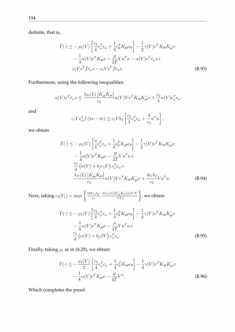
194
definite, that is,
Γ(·) ≤− ρ1(V )
[c2
4eTωeω +
1
4eTθKpθeθ
]− 1
2γ(V )vTKdtK
−ptv
− 1
4α(V )eTKpte−
µ
2TV κTκ− α(V )vT eωs+
c1V sT f eωs− c1V e
T f eωe. (B.93)
Furthermore, using the following inequalities
α(V )vT eωs ≤λN(L)
∣∣K−dtKpt
∣∣c3
α(V )V vTKdtK−ptv +
c3
4α(V )eTωeω
and
c1V eTω f (ss− ee) ≤ c1V bf
[c3
4eTωeω +
4
c3
κTκ
],
we obtain
Γ(·) ≤− ρ1(V )
[a
4eTωeω +
1
4eTθKpθeθ
]− 1
2γ(V )vTKdtK
−ptv
− 1
4α(V )eTKpte−
µ
2TV κTκ+
c3
4
(α(V ) + bfc1V
)eTωeω+
λN(L)∣∣K−dtKpt
∣∣c3
α(V )V vTKdtK−ptv +
4c1bfc3
V κTκ. (B.94)
Next, taking c3(V1) = max
16Tc1bf
µ,
4λN (L)|K−dtKpt|α(V )V
γ(V )
, we obtain
Γ(·) ≤− ρ1(V )
[c2
4eTωeω +
1
4eTθKpθeθ
]− 1
4γ(V )vTKdtK
−ptv
− 1
8α(V )eTKpte−
µ
4TV κTκ+
c3
4
(α(V ) + bfβV
)eTωeω. (B.95)
Finally, taking ρ1 as in (4.29), we obtain
Γ(·) ≤− ρ1(V )
2
[c2
4eTωeω +
1
4eTθKpθeθ
]− 1
4γ(V )vTKdtK
−ptv
− 1
8α(V )eTKpte−
µ
4TV 3. (B.96)
Which completes the proof.

Appendix B 195
B.10 Proof of theorem 4.2
We start observing that the transnational part of the closed-loop system (4.42) admits
the following non-strict Lyapunov-Krasovskii functional candidate
V (θ,Xt, zt) = v>K−1pt v + z>L2z +
∫ 0
−T ∗
∫ t
t+θ
z(s)T z(s)dsdθ (B.97)
where T ∗ = maxi,j Tij.Indeed, in view of the following inequality∫ 0
−T ∗
∫ t
t+θ
z(s)T z(s)dsdθ ≤ T ∗∫ t
t−T ∗|z(s)|2 ds
one can easily establish that V (θ,Xt, zt) is Lyapunov-Krasovskii functional candidate
with respect to Xt. Moreover, the time derivative of V (·) along the trajectories of (4.42)
is given by
V (·) =− 2v>K−1pt Kdtv + 2vTΦ(θ)TA(zt) + T ∗vTv −
∫ t
t−T ∗z(s)T z(s)ds
≤− [2− T ∗λM(KptK−dt)]v
>K−1pt Kdtv −
1
a2N
N∑j=1
N∑i=1
a2ij
∫ t
t−Tijzi(s)
T zi(s)ds+
2vTΦ(θ)TA(zt). (B.98)
Applying Jensen’s inequality, we obtain the following∫ t
t−Tijzi(s)
T zi(s)ds ≤ −1
T ∗ij
∫ t
t−Tijzi(s)
Tds
∫ t
t−Tijzi(s)ds. (B.99)
Moreover, using the inequality
|A(zt)|2 ≤NN∑j=1
N∑i=1
∫ t
t−Tijzi(s)
Tdsa2ij
∫ t
t−Tijzi(s)ds (B.100)
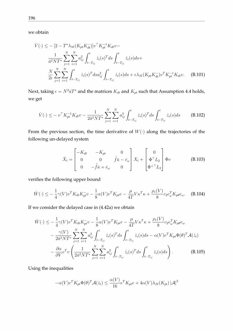
196
we obtain
V (·) ≤− [2− T ∗λM(KptK−dt)]v
>K−1pt Kdtv−
1
a2NT ∗
N∑j=1
N∑i=1
a2ij
∫ t
t−Tijzi(s)
Tds
∫ t
t−Tijzi(s)ds+
N
2ε
N∑j=1
N∑i=1
∫ t
t−Tijzi(s)
Tdsa2ij
∫ t
t−Tijzi(s)ds+ ελM(KptK
−dt)v
TK−1pt Kdtv. (B.101)
Next, taking ε = N2aT ∗ and the matrices Kdt and Kpt such that Assumption 4.4 holds,
we get
V (·) ≤− v>K−1pt Kdtv −
1
2a2NT ∗
N∑j=1
N∑i=1
a2ij
∫ t
t−Tijzi(s)
Tds
∫ t
t−Tijzi(s)ds (B.102)
From the previous section, the time derivative of W (·) along the trajectories of the
following un-delayed system
Xt =
−Kdt −Kpt 0
0 0 ¯fκ− eω0 − ¯fκ+ eω 0
Xt +
0
Φ>L2
Φ⊥>L2
Φv (B.103)
verifies the following upper bound
W (·) ≤− 1
4γ(V )vTKdtK
−ptv −
1
8α(V )eTKpte−
µ
4TV κTκ+
ρ1(V )
8c2e
TωKpθeω. (B.104)
If we consider the delayed case in (4.42a) we obtain
W (·) ≤− 1
4γ(V )vTKdtK
−ptv −
1
8α(V )eTKpte−
µ
4TV κTκ+
ρ1(V )
8c2e
TωKpθeω
− γ(V )
2a2NT ∗
N∑j=1
N∑i=1
a2ij
∫ t
t−Tijzi(s)
Tds
∫ t
t−Tijzi(s)ds− α(V )eTKptΦ(θ)TA(zt)
− ∂α
∂VeTv
(1
2a2NT ∗
N∑j=1
N∑i=1
a2ij
∫ t
t−Tijzi(s)
Tds
∫ t
t−Tijzi(s)ds
). (B.105)
Using the inequalities
−α(V )eTKptΦ(θ)TA(zt) ≤α(V )
16eTKpte+ 4α(V )λM(Kpt) |A|2

Appendix B 197
and
|A|2 ≤ NN∑j=1
N∑i=1
a2ij
∫ t
t−Tijzi(s)
Tds
∫ t
t−Tijzi(s)ds
we obtain
W (·) ≤− 1
4γ(V )vTKdtK
−ptv −
1
16α(V )eTKpte−
µ
4TV κTκ+
ρ1(V )
8c2e
TωKpθeω. (B.106)
On the other hand, the time derivative ρ1(V )Z(Xr) along the following un-delayed
system
Xr =
[0 IN
−Kpθ −Kdθ
]Xr +
[bf¯f
] (eΦ>L2 + sΦ⊥>L2
)Φv (B.107)
satisfies the following upper bound
d
dt(ρ1(V )Z(Xr)) ≤− ρ1(V )
[c2
4eTωKdθeω +
1
4eTθKpθeθ
]+
1
2ρ2(V )vTKdtK
−ptv
− Z(Xr)V . (B.108)
If we consider the delayed case as in (4.42b), we obtain
d
dt(ρ1(V )Z(Xr)) ≤− ρ1(V )
[c2
4eTωKdθeω +
1
4eTθKpθeθ
]+
1
2ρ2(V )vTKdtK
−ptv + 2ρ1(V )Kptc2e
Tωκd + ρ1(V )Kpte
Tθ κd
− Z(Xr)
(− 1
2a2NT ∗
N∑j=1
N∑i=1
a2ij
∫ t
t−Tijzi(s)
Tds
∫ t
t−Tijzi(s)ds
).
(B.109)
Using the fact that
κd =1
2
|A1|2
...
|AN |2
+ eΦTA(zt) + sΦ⊥TA(zt)
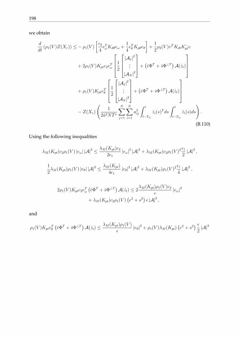
198
we obtain
d
dt(ρ1(V )Z(Xr)) ≤− ρ1(V )
[c2
4eTωKdθeω +
1
4eTθKpθeθ
]+
1
2ρ2(V )vTKdtK
−ptv
+ 2ρ1(V )Kptc2eTω
1
2
|A1|2
...
|AN |2
+(eΦT + sΦ⊥T
)A(zt)
+ ρ1(V )KpteTθ
1
2
|A1|2
...
|AN |2
+(eΦT + sΦ⊥T
)A(zt)
− Z(Xr)
(1
2a2NT ∗
N∑j=1
N∑i=1
a2ij
∫ t
t−Tijzi(s)
Tds
∫ t
t−Tijzi(s)ds
).
(B.110)
Using the following inequalities
λM(Kpt)c2ρ1(V ) |eω| |A|2 ≤λM(Kpt)c2
2ε1|eω|2 |A|2 + λM(Kpt)c2ρ1(V )2 ε1
2|A|2 ,
1
2λM(Kpt)ρ1(V ) |eθ| |A|2 ≤
λM(Kpt)
4ε1|eθ|2 |A|2 + λM(Kpt)ρ1(V )2 ε1
4|A|2 ,
2ρ1(V )Kptc2eTω
(eΦT + sΦ⊥T
)A(zt) ≤ 2
λM(Kpt)ρ1(V )c2
ε|eω|2
+ λM(Kpt)c2ρ1(V )(e2 + s2
)ε |A|2 ,
and
ρ1(V )KpteTθ
(eΦT + sΦ⊥T
)A(zt) ≤
λM(Kpt)ρ1(V )
ε|eθ|2 + ρ1(V )λM(Kpt)
(e2 + s2
) ε2|A|2

Appendix B 199
we obtain
d
dt(ρ1(V )Z(Xr)) ≤− ρ1(V )
[c2
4eTωKdθeω +
1
4eTθKpθeθ
]+
1
2ρ2(V )vTKdtK
−ptv
+λM(Kpt)ρ1(V )
ε(2c2 + 1)
(|eω|2 + |eθ|2
)+λM(Kpt)
2ε1
(c2 +
1
2
)(|eω|2 + |eθ|2
)|A|2
+ λM(Kpt)ρ1(V )
[(c2 +
1
2
)ρ1(V )
ε12
+
(c2 +
1
2
)λN(L)V ε
]|A|2
− Z(Xr)
2a2NT ∗
(N∑j=1
N∑i=1
a2ij
∫ t
t−Tijzi(s)
Tds
∫ t
t−Tijzi(s)ds
). (B.111)
Taking ε1 = c5, ε = c6, and using the inequalities
Z ≥ min 1, λm(Kpθ)(e>θ eθ + e>ω eω
)and
|A|2 ≤ NN∑j=1
N∑i=1
a2ij
∫ t
t−Tijzi(s)
Tds
∫ t
t−Tijzi(s)ds
we obtain
d
dt(ρ1(V )Z(Xr)) ≤− ρ1(V )
[3c2
16eTωKdθeω +
3
16eTθKpθeθ
]+
1
2ρ2(V )vTKdtK
−ptv
+ λM(Kpt)ρ1(V )
[(c2 +
1
2
)ρ1(V )
ε12
+
(c2 +
1
2
)λN(L)V ε
]|A|2 .
(B.112)
Finally, we conclude
Γ(·) ≤− 1
8γ(V )vTKdtK
−ptv −
1
16α(V )eTKpte−
µ
8TV κTκ
− ρ1(V )
[c2
16eTωKdθeω +
1
16eTθKpθeθ
]. (B.113)
Which completes the proof.
B.11 Proof of theorem 4.3
First, since ρ1(V ) and ρ2(V ), in (4.60) and (4.62) respectively, are strictly positive func-
tions and radially unbounded, positive definiteness of Γ is ensured using the fact that

200
Γ(t, 0, 0) = 0, for all t ≥ 0,
W ≥ γ(V )V,
W ≤ γ(V )V + V κ>(e, s)Υq2(t)κ(e, s) + 2c1bfλN(L)V 2 + 2 (λN(L) + |Kpt|)α(V )V,
and
c2
2
(eTθ Leθ + eTωeω + eTαK
−I eα
)≤ Z ≤ 2c2
(eTθ Leθ + eTωeω + eTαK
−I eα
).
Furthermore, since the translational part of (4.57) is similar to the one presented in
(4.57a), it becomes straightforward to conclude the following
W (·) ≤− 1
2γ(V )vTKdtK
−ptv −
1
4α(V )eTKpte−
µ
2TV κTκ
− α(V )vT eωs+ c1V sT f eωs− f c1V e
T f eωe. (B.114)
Then, using the following inequalities
α(V )vT eωs ≤λN(L)
∣∣K−dtKpt
∣∣σ
α(V )V vTKdtK−ptv +
σ
4α(V )eTωeω,
c1V eTω f (ss− ee) ≤ c1V bf
[σ
4eTωeω +
4
σκTκ
],
and taking σ = max
16Tc1bq
µ,
4λN (L)|K−dtP |α(V )V
γ(V )
, we obtain
W (·) ≤− 1
4γ(V )vTKdtK
−ptv −
1
8α(V )eTKpte−
µ
4TV κTκ+
σ
4(α(V ) + bqc1V ) eTωeω
(B.115)
and
W (·) ≤− 1
4γ(V )vTKdtK
−ptv −
1
8α(V )eTKpte−
µ
4TV κTκ+
ρ1(V )
8c5e
TωKIeω. (B.116)
Notice that the function Z(Xr) is a strict Lyapunov function for the following system
Xr =
0 IN 0
−L 0 IN
0 −KI −Kα
Xr, (B.117)

Appendix B 201
it’s time derivative along the trajectories of (B.117) satisfies
Z(Xr) ≤ −1
2
[c2α
TK−I Kαα + c2eTωKIeω + eTθ L
2eθ]
(B.118)
and along the trajectories of (4.57) it satisfies
d
dt(ρ1(V )Z(Xr)) ≤−
1
2ρ1(V )
[c2e
TαK
−I Kαeα + c5e
TωKIeω + eTθ L
2eθ]
+ ρ1eTθ L [2c2q + ¯q]
(eΦTL2 + sΦ⊥TL2
)Φv
+ ρ1eTω [2c2
¯q + Lbq + c5¯q](eΦTL2 + sΦ⊥TL2
)Φv
+ ρ1eTα
[2K−I
¯qc2 + c5¯q] (eΦTL2 + sΦ⊥TL2
)Φv. (B.119)
Using the following inequalities
eTθ L [2c2q + ¯q](eΦTL2 + sΦ⊥TL2
)Φv ≤ 1
4eTθ L
2eθ
+ 2b2qλM(L) (2c2 + 1)2 V
[∣∣ΦTLΦ∣∣∞ +
∣∣Φ⊥TLΦ∣∣∞
] ∣∣K−dtKpt
∣∣ vTKdtK−ptv, (B.120)
eTω [2c2¯q + Lbq + c5
¯q](eΦTL2 + sΦ⊥TL2
)Φv ≤ 1
4c5e
TωKIeω
+ 2b2qλM(L)
λM(K−I )
c5
(2c2 + c5 + λN(L))2 V
×[∣∣ΦTLΦ
∣∣∞ +
∣∣Φ⊥TLΦ∣∣∞
] ∣∣K−dtKpt
∣∣ vTKdtK−ptv, (B.121)
and
ρ1eTα
[2K−I
¯qc2 + c5¯q] (eΦTL2 + sΦ⊥TL2
)Φv ≤ 1
4c2e
TαK
−I Kαeα
+ 2b2qλM(L)
λM(K−αKI)
c2
(2c2λM(K−I ) + c5
)2V
×[∣∣ΦTLΦ
∣∣∞ +
∣∣Φ⊥TLΦ∣∣∞
] ∣∣K−dtKpt
∣∣ vTKdtK−ptv (B.122)
we obtain
d
dt(ρ1(V )Z(Xr)) ≤−
1
4ρ1(V )
[c2e
TαK
−I Kαeα + c5e
TωKIeω + eTθ L
2eθ]
+ 2b2qρ1(V )λM(L)
[(2c2 + 1)2 +
λM(K−I )
c5
(2c2 + c5 + λN(L))2
+λM(K−αKI)
c2
(2c2λM(K−I ) + c5
)2]V
×[∣∣ΦTLΦ
∣∣∞ +
∣∣Φ⊥TLΦ∣∣∞
] ∣∣K−dtKpt
∣∣ vTKdtK−ptv, (B.123)
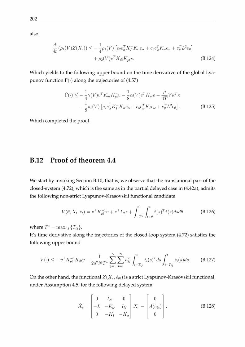
202
also
d
dt(ρ1(V )Z(Xr)) ≤−
1
4ρ1(V )
[c2e
TαK
−I Kαeα + c5e
TωKωeω + eTθ L
2eθ]
+ ρ2(V )vTKdtK−ptv. (B.124)
Which yields to the following upper bound on the time derivative of the global Lya-
punov function Γ(·) along the trajectories of (4.57)
Γ(·) ≤− 1
4γ(V )vTKdtK
−ptv −
1
8α(V )eTKpte−
µ
4TV κTκ
− 1
8ρ1(V )
[c2e
TαK
−I Kαeα + c5e
TωKIeω + eTθ L
2eθ]. (B.125)
Which completed the proof.
B.12 Proof of theorem 4.4
We start by invoking Section B.10, that is, we observe that the translational part of the
closed-system (4.72), which is the same as in the partial delayed case in (4.42a), admits
the following non-strict Lyapunov-Krasovskii functional candidate
V (θ,Xt, zt) = v>K−1pt v + z>L2z +
∫ 0
−T ∗
∫ t
t+θ
z(s)T z(s)dsdθ. (B.126)
where T ∗ = maxi,j Tij.It’s time derivative along the trajectories of the closed-loop system (4.72) satisfies the
following upper bound
V (·) ≤− v>K−1pt Kdtv −
1
2a2NT ∗
N∑j=1
N∑i=1
a2ij
∫ t
t−Tijzi(s)
Tds
∫ t
t−Tijzi(s)ds. (B.127)
On the other hand, the functional Z(Xr, eθt) is a strict Lyapunov-Krasovskii functional,
under Assumption 4.5, for the following delayed system
Xr =
0 IN 0
−L −Kω IN
0 −KI −Kα
Xr −
0
A(eθt)
0
. (B.128)
Appendix B 203
Indeed, we have
Z ≥ c2
2
(eTθ Leθ + eTωeω + eTαK
−I eα
),
Z ≤ 2c2
(eTθ Leθ + eTωeω + eTαK
−I eα
)+ 2c5T
∗∫ t
t−T ∗|eθ(s)|2 ds.
and the time derivative of Z(Xr, θt) along trajectories of (B.128) is given by
Z(·) =− 2c2
[eTαK
−I Kαeα + eTωKωeω
]− eTθ L2eθ − eTθ LKωeω + eTθ Leα + eTωLeω
− eTθ LA(eθt)− 2c2eTωA(eθt) + c5T
∗eTθ eθ − c5
∫ t
t−T ∗eTθ (s)eθ(s)ds. (B.129)
Using the fact that Kω > In both with the following inequalities
eTθ Leα ≤1
2εeTθ L
2eθ +ε
2λM(KIK
−α )eTαK
−I Kαeα,
eTωLeω ≤ λN(L)eTωKωeω,
−2c2eTωA(eθt) ≤ ε1c2e
TωKωeω +
c2
ε1|A(eθt)|2 ,
eTθ LA(eθt) ≤1
2εeTθ L
2eθ +ε
2|A(eθt)|2 ,
eTθ LKωeω ≤1
2εeTθ L
2eθ +ελM(Kω)
2,
|A(eθt)|2 ≤ NN∑j=1
N∑i=1
(∫ t
t−Tijeθj(s)ds
)2
a2ij,
∫ t
t−T ∗eTθ (s)eθ(s)ds ≥
1
a2N
N∑j=1
N∑i=1
a2ij
∫ t
t−Tije2θj(s)ds,
∫ t
t−Tija2ij e
2θj(s)ds ≥
1
T ∗
(∫ t
t−Tijeθj(s)ds
)2
a2ij,
taking ε1 = 12, ε = 3 and using Assumption 4.5, we obtain
Z(·) =− 1
2c2
[eTαK
−I Kαeα + eTωKωeω
]− 1
2eTθ L
2eθ. (B.130)
Since V is Lyapunov Krasovskii functional candidate, Γ(t, 0, 0, 0, 0) = 0, for all t ≥ 0,
and the following inequalities hold
W ≥ γ(V )V,
W ≤ γ(V )V + V κ>(e, s)Υq2(t)κ(e, s) + 2c1bfλN(L)V 2 + 2 (λN(L) + |Kpt|)α(V )V,
then Γ is Lyapunov Krasovskii functional candidate for the closed-loop system.

204
Using the previous section, the time derivative of W (·) along the trajectories of the
following un-delayed system
Xt =
−Kdt −Kpt 0
0 0 ¯fκ− eω0 − ¯fκ+ eω 0
Xt +
0
Φ>L2
Φ⊥>L2
Φv −
KptΦ(θ)T
0
0
A(zt) (B.131)
satisfies
W (·) ≤− 1
4γ(V )vTKdtK
−ptv −
1
16α(V )eTKpte−
µ
4TV κTκ+
ρ1(V )
8c2e
TωKpθeω. (B.132)
Moreover, the time derivative ρ1(V )Z(Xr) along the following system
Xr =
0 IN 0
−L −Kω IN
0 −KI −Kα
Xr −
0
A(eθt)
0
(B.133)
satisfies the following upper bound
d
dt(ρ1(V )Z(Xr)) ≤−
ρ1(V )
2c2
[eTαK
−I Kαeα + eTωKωeω
]− ρ1(V )
2eTθ L
2eθ. (B.134)
Now, if we consider the delayed system in (4.72b) when B(t) = 0, which has the fol-
lowing form
Xr =
0 IN 0
−L −Kω IN
0 −KI −Kα
Xr −
0
A(eθt)
0
+
bq¯q
¯q
(eΦ>L2 + sΦ⊥>L2
)Φv
−
0
Kω (¯q + bqK−ωD)
p
κd(e, s, θ, zt), (B.135)
M :=(eΦ>L2 + sΦ⊥>L2
)Φ.
Appendix B 205
We obtain
d
dt(ρ1(V )Z(Xr)) ≤−
ρ1(V )
2c2
[eTαK
−I Kαeα + eTωKωeω
]− ρ1(V )
2eTθ L
2eθ
− 2c2ρ1(V )[eTωKω
(¯q + bqK
−ωD)κd + peTαK
−I κd
]− ρ1(V )eTθ LKω
(¯q + bqK
−ωD)κd
+ ρ1(V )c5T∗ [vTMb2
qMv + 2eTωbqMv]
+ ρ1(V )eTθ L (2c2q + ¯q)Mv + ρ1(V )eTω (c2¯q + Lbq)Mv
+ ρ1(V )eTα(2c2K
−I
¯q)Mv
− Z(Xr)
(1
2a2NT ∗
N∑j=1
N∑i=1
a2ij
∫ t
t−Tijzi(s)
Tds
∫ t
t−Tijzi(s)ds
).
(B.136)
Using the following equality
κd =1
2
|A1|2
...
|AN |2
+ eΦTA(zt) + sΦ⊥TA(zt)
we obtain
d
dt(ρ1(V )Z(Xr)) ≤−
ρ1(V )
2c2
[eTαK
−I Kαeα + eTωKωeω
]− ρ1(V )
2eTθ L
2eθ
− 2c2ρ1(V )[eTωKω
(¯q + bqK
−ωD)
+ peTαK−I
]∗
1
2
|A1|2
...
|AN |2
+ eΦTA(zt) + sΦ⊥TA(zt)
− ρ1(V )eTθ LKω
(¯q + bqK
−ωD)1
2
|A1|2
...
|AN |2
+ eΦTA(zt) + sΦ⊥TA(zt)
+ ρ1(V )c5T
∗ [vTMb2qMv + 2eTωbqMv
]+ ρ1(V )eTθ L (2c2q + ¯q)Mv + ρ1(V )eTω (c2
¯q + Lbq)Mv
+ ρ1(V )eTα(2c2K
−I
¯q)Mv
− Z(Xr)
(1
2a2NT ∗
N∑j=1
N∑i=1
a2ij
∫ t
t−Tijzi(s)
Tds
∫ t
t−Tijzi(s)ds
).
(B.137)
206
Using the following inequalities
c2ρ1(V )bq(1 + λM(K−ωD)
)|Kωeω| |A|2 ≤
c2bq2ε1
λM(Kω)2 |eω|2 |A|2+c2bq
2
(1 + λM(K−ωD)
)2,
∗ε1 |A|2 ρ1(V )2,
2c2ρ1(V )eTωKω
(¯q + bqK
−ωD) (eΦT + sΦ⊥T
)A ≤ 2
c2
ερ1(V )bqe
TωKωeω+
εc2
(1 + λM(K−ωD)
)2ρ1bqλM(Kω)
(e2 + s2
)|A|2 ,
c2ρ1(V )bp∣∣K−I eα∣∣ |A|2 ≤ c2bp
2ε1
∣∣K−I eα∣∣2 |A|2 +c2bpε1
2|A|2 ρ2
1(V ),
2c2ρ1(V )eTαK−I p(eΦT + sΦ⊥T
)A ≤ 2
c2λM(K−αK−I )
ερ1(V )bqe
TαKαK
−I eα
+εc2bqρ1(V )(e2 + s2
)|A|2 ,
ρ1(V ) |Leθ|λM(Kω)(1 + λM(K−ωD)
)bq |A|2 ≤ |A|2 λM(Kω)bq
1
2ε1|Leθ|2
+1
2λM(Kω)bq
(1 + λM(K−ωD)
)2 |A|2 ε1,
ρ1(V )eTθ LKω
(¯q + bqK
−ωD) (eφT + sφ⊥T
)A ≤ λM(Kω)ρ1(V )
bqε
(eTθ L
2eθ)
+
λM(Kω)
2
(1 + λM(K−ωD)
)2ε(e2 + s2
)bq |A|2 ρ1(V ),
ρ1(V )eTθ L (2c2q + ¯q)Mv ≤ ρ1(V )bq2ε
∣∣eTθ L∣∣2+bqε
2ρ1(V ) (2c2 + 1)2 |M |2
∣∣K−dtKpt
∣∣ vTKdtK−ptv,
ρ1(V )eTω (c2¯q + Lbq)Mv ≤ ρ1(V )
c2bq2ε
eTωKωeω +bqε
2c2
ρ1(V )λM(Kω) (2c2 + λN(L))2
∗ |M |2∣∣K−dtKpt
∣∣ vTKdtK−ptv,
ρ1(V )eTα(2c2K
−I
¯q)Mv ≤ ρ1(V )
c2bqεeTαKαK
−I eα + ερ1(V )
(c2λM(K−I K
−α )bq
)∗ |M |2
∣∣K−dtKpt
∣∣ vTKdtK−ptv
c5T∗ρ1(V )vTMT b2
qMv ≤ c5T∗ρ1(V )b2
q |M |2∣∣KdtK
−pt
∣∣ vTKdtK−ptv,
2c5T∗ρ1(V )eTωbqMv ≤ c5T
∗ρ1(V )bqε
eTωKωeω + ρ1(V )λM(K−ω )εbqc5T∗ |M |2
∗∣∣K−dtKpt
∣∣ vTKdtK−ptv,
taking ε1 = c7, ε = c6 and using the inequalities
Z ≥ c2
2
(eTθ Leθ + eTωeω + eTαK
−I eα
),
Bibliography 207
|A|2 ≤ N
N∑j=1
N∑i=1
a2ij
∫ t
t−Tijzi(s)
Tds
∫ t
t−Tijzi(s)ds
we obtain
d
dt(ρ1(V )Z(Xr)) ≤−
ρ1(V )
4c2
[eTαK
−I Kαeα + eTωKωeω
]− ρ1(V )
4eTθ L
2eθ
+1
2ρ2(V )vtKdtK
−ptv +
1
2ρ2(V )
N∑j=1
N∑i=1
a2ij
∫ t
t−Tijzi(s)
Tds
∫ t
t−Tijzi(s)ds.
(B.138)
Finally, we obtain
Γ ≤− ρ1(V )
8
[c2e
TαK
−I Kαeα + c2e
TωKωeω + eTθ L
2eθ]
− 1
4γ(V )v>KdtK
−1pt v −
1
16α(V )e>Kpte−
µ
4TV 3.
(B.139)
Which completes the proof.

208

Bibliography
[1] A. Abdessameud, I. G. Polushin, and A. Tayebi. Synchronization of lagrangian
systems with irregular communication delays. IEEE Transactions on Automatic
Control, 59(1):187–193, 2014.
[2] J. H. Ahrens and H. K. Khalil. High-gain observers in the presence of measure-
ment noise: A switched-gain approach. Automatica, 45(4):936–943, 2009.
[3] A. Ajorlou, M.M. Asadi, A. G. Aghdam, and S. Blouin. Distributed consensus
control of unicycle agents in the presence of external disturbances. Systems &
Control Letters, 82:86–90, 2015.
[4] M. R. Akella and S. Srikant. Persistence filter based attitude stabilization of
microsatellites with variable amplitude thrusters. In 20th AAS/AIAA Space Flight
Mechanics Meeting, 2010.
[5] C. I. Aldana, E. Romero, E. Nuno, and L. Basanez. Pose consensus in networks
of heterogeneous robots with variable time delays. International Journal of Robust
and Nonlinear Control, 25(14):2279–2298, 2015.
[6] N. Alvarez-Jarquın and A. Lorıa. Consensus under persistent interconnections
in a ring topology: a small gain approach. In Proc. Math. Theory of Networks and
Systems , pages 524–529, Groningen, The Netherlands, 2014.
[7] B. D. O. Anderson, R.R. Bitmead, C.R. Johnson, Jr., P.V. Kokotovic, R.L. Kosut,
I. Mareels, L. Praly, and B.D. Riedle. Stability of adaptive systems. The MIT Press,
Cambridge, MA, USA, 1986.
[8] D. Angeli, B. Ingalls, E. D. Sontag, and Y. Wang. Separation principles for input-
output and integral-input-to-state stability. SIAM J. on Contr. and Opt., 43(1):256–
276, 2004.
[9] D. Angeli, E. D. Sontag, and Y. Wang. A characterization of integral input-to-
state stability. IEEE Trans. on Automat. Contr., 45(6):1082–1097, 2000.
209

210
[10] A. Astolfi. Exponential stabilization of a wheeled mobile robot via discontinuous
control. ASME J. Dyn. Syst. Meas. Contr., 121(1):121–126, 1999.
[11] K. J. Astrom and Bohn. Numerical identification of linear dynamic systems from
normal operating records. In P. H. Hammond, editor, Proc. of the 2nd IFAC
Symp. on Theory of Self-adaptive Control Systems, pages 96–111, Nat. Phys.
Lab., Teddington, England, 1965.
[12] A. Bautista-Castillo, C. Lopez-Franco, and E. Nuno. Consensus-based formation
control for multiple nonholonomic robots. In Accepted in 2016 IEEE International
Autumn Meeting on Power, Electronics and Computing (ROPEC). IEEE, 2016.
[13] D. J. W. Belleter and K. Y. Pettersen. Leader–follower synchronisation for a class
of underactuated systems. In Nonlinear Systems, pages 157–179. Springer Inter-
national Publishing, 2017.
[14] G. Besancon. A viewpoint on observability and observer design for nonlinear systems,
chapter in New directions in nonlinear observer design. Lecture Notes in Control
and Information Sciences. Springer Verlag, H. Nijemeijer, T. I. Fossen, eds., Lon-
don, 1999.
[15] R. Brockett. Asymptotic stability and feedback stabilization. In R. S. Millman
R. W. Brocket and H. J. Sussmann, editors, Differential geometric control theory,
pages 181–191. Birkhauser, 1983.
[16] R. Brockett. The rate of descent for degenerate gradient flows. In Proc. Math.
Theory of Networks and Systems, 2000.
[17] A. Chaillet, D. Angeli, and H. Ito. Combining iISS and ISS with respect to small
inputs: the strong iISS property. IEEE Trans. on Automat. Contr., 59(9):2518–2524,
2014.
[18] A. Chaillet, D. Angeli, and H. Ito. Strong iISS is preserved under cascade inter-
connection. Automatica, 50(9):2424–2427, 2014.
[19] A. Chaillet, Y. Chitour, A. Lorıa, and M. Sigalotti. Uniform stabilization for lin-
ear systems with persistency of excitation. The neutrally stable and the double
integrator cases. Math. of Cont. Sign. and Syst., 20(2):136–156, 2008.
[20] N. R. Chowdhury, S. Sukumar, M. Maghenem, and A. Lorıa. On the estimation
of algebraic connectivity in graphs with persistently exciting interconnections.
Int. J. of Contr., 2016. Submitted.

Bibliography 211
[21] L. Consolini, F. Morbidi, D. Prattichizzo, and M. Tosques. Leader–follower for-
mation control of nonholonomic mobile robots with input constraints. Automat-
ica, 44(5):1343–1349, 2008.
[22] J. Cortes, S. Martınez, and F. Bullo. Robust rendezvous for mobile autonomous
agents via proximity graphs in arbitrary dimensions. IEEE Transactions on Auto-
matic Control, 51(8):1289–1298, 2006.
[23] C. Canudas de Wit, H. Khennouf, C. Samson, and O. J. Sørdalen. ”Nonlinear
control design for mobile robots”, volume 11 of Robotics and Automated Systems,
chapter Recent Trends in Mobile Robots. World Scientific, Y. F. Zheng, ed., Lon-
don, 1993.
[24] D. V. Dimarogonas and K. J. Kyriakopoulos. On the rendezvous problem
for multiple nonholonomic agents. IEEE Transactions on Automatic Control,
52(5):916–922, 2007.
[25] K. D. Do. Formation tracking control of unicycle-type mobile robots. In Proceed-
ings 2007 IEEE International Conference on Robotics and Automation, pages 2391–
2396, April 2007.
[26] K. D. Do, Z.-P. Jiang, and J. Pan. A global output-feedback controller for simul-
taneous tracking and stabilization of unicycle-type mobile robots. IEEE Trans.
on Robotics Automat., 20(3):589–594, 2004.
[27] K. D. Do, Z.-P. Jiang, and J. Pan. Simultaneous tracking and stabilization of
mobile robots: an adaptive approach. IEEE Trans. on Automat. Contr., 49(7):1147–
1152, 2004.
[28] K. D. Do and J. Pan. Nonlinear formation control of unicycle-type mobile robots.
J. Rob. and Aut. Syst., 55(3):191–204, 2007.
[29] A. Dong and J. A. Farrell. Cooperative control of multiple nonholonomic mobile
agents. IEEE Trans. on Automat. Contr., 53(6):1434–1447, 2008.
[30] W. Dong. Distributed tracking control of networked chained systems. Int. J. of
Contr., 12(86):2159–2174, 2013.
[31] W. Dong and J. A. Farrell. Consensus of multiple nonholonomic systems. In 47th
IEEE Conference on Decision and Control., pages 2270–2275. IEEE, 2008.
[32] Y. Eun and H. Bang. Cooperative control of multiple unmanned aerial vehicles
using the potential field theory. Journal of Aircraft, 43(6):1805–1814, 2006.
212
[33] E. Fridman. Tutorial on lyapunov-based methods for time-delay systems. Euro-
pean Journal of Control, 20(6):271–283, 2014.
[34] T. Fukao, H. Nakagawa, and N. Adachi. Adaptive tracking control of a nonholo-
nomic mobile robot. IEEE Trans. on Robotics Automat., 16(5):609–615, 2000.
[35] H. Goldstein. Classical Mecanics. Adisson Wesley, 1974.
[36] W. Hahn. Stability of motion. Springer-Verlag, New York, 1967.
[37] J. Hendrickx and J. N. Tsitsiklis. Convergence of type-symmetric and cut-
balanced consensus seeking systems. IEEE Trans. on Automat. Contr., 58(1):214–
218, 2013.
[38] J. M. Hendrickx and J. N. Tsitsiklis. A new condition for convergence in
continuous-time consensus seeking systems. In Proc. 50th. IEEE Conf. on Deci-
sion Contr. and 15th. Europ. Contr. Conf., pages 5070–5075, 2011.
[39] K. h.Tan and M. A. Lewis. Virtual structures for high-precision cooperative mo-
bile robot control. Autonomous Robots, 4:387–403, 1997.
[40] Q. Hui, W. M. Haddad, and S. P. Bhat. Finite-time semistability and consen-
sus for nonlinear dynamical networks. IEEE Transactions on Automatic Control,
53(8):1887–1900, 2008.
[41] P. Ioannou and J. Sun. Robust adaptive control. Prentice Hall, New Jersey, USA,
1996.
[42] H. Ito. A Lyapunov approach to cascade interconnection of integral input-to-
state stable systems. IEEE Trans. on Automat. Contr., 55(3):702–708, 2010.
[43] A. Jadbabaie, J. Lin, and A. S. Morse. Coordination of groups of mobile au-
tonomous agents using nearest neighbor rules. IEEE Trans. on Automat. Contr.,
48(6):988–1001, 2003.
[44] Z.-P. Jiang, E. Lefeber, and H. Nijmeijer. Saturated stabilization and tracking of
a nonholonomic mobile robot. Syst. & Contr. Letters, 42(5):327–332, 2001.
[45] Z.-P. Jiang and H. Nijmeijer. Tracking control of mobile robots: A case study in
backstepping. Automatica, 33(7):1393–1399, 1997.
[46] Y. Kanayama, Y. Kimura, F. Miyazaki, and T. Naguchi. A stable tracking control
scheme for an autonomous vehicle. In Proc. IEEE Conf. Robotics Automat., pages
384–389, 1990.

Bibliography 213
[47] H. Khalil. Nonlinear systems. Macmillan Publishing Co., 2nd ed., New York,
1996.
[48] H. K. Khalil. Nonlinear systems. Prentice hall New Jersey, third edition edition,
2002.
[49] I. Kolmanovsky and N. H. McClamroch. Developments in nonholonomic con-
trol problems. IEEE Control Systems Magazine, 15(6):20–36, 1995.
[50] T. C. Lee. On the equivalence relations of detectability and PE conditions with
applications to stability analysis of time-varying systemss. In Proc. IEEE Ameri-
can Control Conference, June 2003.
[51] T. C. Lee and B. S. Chen. A general stability criterion for time-varying sys-
tems using a modified detectability condition. IEEE Trans. on Automat. Contr.,
47(5):797–802, 2002.
[52] T-C. Lee, K-T. Song, C-H. Lee, and C-C. Teng. Tracking control of unicycle-
modeled mobile robots using a saturation feedback controller. IEEE Trans. Contr.
Syst. Technol., 9(2):305–318, 2001.
[53] E. Lefeber, K. Y. Pettersen, and H. Nijmeijer. Tracking control of an underactu-
ated ship. IEEE Trans. Contr. Syst. Technol., 11(1):52–61, 2003.
[54] Z. Li, W. Ren, X. Liu, and M. Fu. Consensus of multi-agent systems with general
linear and lipschitz nonlinear dynamics using distributed adaptive protocols.
IEEE Transactions on Automatic Control, 58(7):1786–1791, 2013.
[55] Z. Lin, B. Francis, and M. Maggiore. Necessary and sufficient graphical con-
ditions for formation control of unicycles. IEEE Trans. on Automat. Contr.,
50(1):121–127, 2005.
[56] K. Liu, Z. Ji, and W. Ren. Necessary and sufficient conditions for consensus of
second-order multiagent systems under directed topologies without global gain
dependency. IEEE Transactions on Cybernetics, 2016.
[57] X. Liu, Y. Guo, and P. Lu. Robust attitude coordination control for satellite forma-
tion with matched perturbations and measurement noises. In American Control
Conference (ACC), 2014, pages 3893–3898. IEEE, 2014.
[58] A. Lorıa. Explicit convergence rates for MRAC-type systems. Automatica,
40(8):1465–1468, 2004.
214
[59] A. Lorıa. From feedback to cascade-interconnected systems: Breaking the loop.
In Proc. 47th. IEEE Conf. Decision Contr., pages 4109–4114, Cancun, Mex., 2008.
[60] A. Lorıa. A linear time-varying controller for synchronization of lu chaotic sys-
tems with one input. IEEE Trans. on Circ. Syst. II: Express Briefs, 56(8):674–678,
2009.
[61] A. Lorıa, A. Chaillet, G. Besancon, and Y. Chitour. On the PE stabilization of
time-varying systems: open questions and preliminary answers. In Proc. 44th.
IEEE Conf. Decision. Contr, pages 6847–6842, 2005.
[62] A. Lorıa, J. Dasdemir, and N. Alvarez-Jarquin. Leader-follower formation con-
trol of mobile robots on straight paths. IEEE Trans. on Contr. Syst. Techn.,
24(2):727–732, 2016.
[63] A. Lorıa and E. Panteley. Uniform exponential stability of linear time-varying
systems: revisited. Syst. & Contr. Letters, 47(1):13–24, 2002.
[64] A. Lorıa, E. Panteley, and K. Melhem. UGAS of skew-symmetric time-varying
systems: application to stabilization of chained form systems. European J. of
Contr., 8(1):33–43, 2002.
[65] A. Lorıa E. Panteley, D. Popovic, and A. Teel. δ-persistency of excitation: a
necessary and sufficient condition for uniform attractivity. In Proc. 41th. IEEE
Conf. Decision Contr., pages 3506–3511, Las Vegas, CA, USA, 2002. Paper no.
REG0623 .
[66] A. Lorıa, E. Panteley, D. Popovic, and A. Teel. A nested Matrosov theorem
and persistency of excitation for uniform convergence in stable non-autonomous
systems. IEEE Trans. on Automat. Contr., 50(2):183–198, 2005.
[67] A. Lorıa, E. Panteley, and A. Teel. A new persistency-of-excitation condition for
UGAS of NLTV systems: Application to stabilization of nonholonomic systems.
In Proc. 5th. European Contr. Conf., pages 1363–1368, Karlsruhe, Germany, 1999.
[68] A. Lorıa, E. Panteley, and A. Zavala. Adaptive observers for robust synchroniza-
tion of chaotic systems. IEEE Trans. on Circ. Syst. I: Regular Papers, 56(12):2703–
2716, 2009.
[69] M. Lovera and A. Astolfi. Spacecraft attitude control using magnetic actuators.
Automatica, 40(8):1405–1414, 2004.
Bibliography 215
[70] M. Maghenem, A. Lorıa and E. Panteley. Lyapunov-based formation-tracking
control of nonholonomic systems under persistency of excitation. IFAC-
PapersOnLine, 49(18):404–409, 2016. Presented at IFAC NOLCOS 2016, Monterey,
CA, USA.
[71] M. Maghenem, A. Lorıa, and E. Panteley. Global tracking-stabilization con-
trol of mobile robots with parametric uncertainty. In IFAC World Congress 2017,
Toulouse, France, 2017. Accepted.
[72] M. Malisoff and F. Mazenc. Constructions of Strict Lyapunov functions. Springer
Verlag, London, 2009.
[73] S. Martin and A. Girard. Continuous-time consensus under persistent connec-
tivity and slow divergence of reciprocal interaction weights. SIAM Journal on
Control and Optimization, 2013.
[74] F. Mazenc. Strict Lyapunov functions for time-varying systems. Automatica,
39(2):349–353, 2003.
[75] F. Mazenc, M. de Queiroz, and M. Malisoff. Uniform global asymptotic stability
of a class of adaptively controlled nonlinear systems. IEEE Trans. on Automat.
Contr., 54(5):1152–1158, 2009.
[76] F. Mazenc and D. Nesic. Lyapunov functions for time-varying systems satisfy-
ing generalized conditions of matrosov theorem. Math. of Cont. Sign. and Syst.,
19(2):151–182, 2007.
[77] M. Mesbahi and M. Egerstedt. Graph theoretic methods in multiagent networks.
Princeton University Press, 2010.
[78] Z. Miao and Y. Wang. Adaptive control for simultaneous stabilization and track-
ing of unicycle mobile robots. Asian. J. Contr., 2015.
[79] L. Moreau. Stability of continuous-time distributed consensus algorithms. In
Proc. 43rd. IEEE Conf. Decision. Contr., volume 4, pages 3998–4003, 2004.
[80] L. Moreau. Stability of multiagent systems with time-dependent communication
links. IEEE Trans. on Automat. Contr., 50(2):169–182, 2005.
[81] L. Moreau. Stability of multiagent systems with time-dependent communication
links. IEEE Transactions on Automatic Control, 50(2):169–182, Feb 2005.
216
[82] A. P. Morgan and K. S. Narendra. On the stability of nonautonomous differential
equations x = [A + B(t)]x with skew-symmetric matrix B(t). SIAM J. on Contr.
and Opt., 15(1):163–176, 1977.
[83] A. P. Morgan and K. S. Narendra. On the uniform asymptotic stability of certain
linear nonautonomous differential equations. SIAM J. on Contr. and Opt., 15(1):5–
24, 1977.
[84] P. Morin and C. Samson. Application of backstepping techniques to the time-
varying exponential stabilisation of chained form systems. European J. of Contr.,
3(1):15–36, 1997.
[85] P. Morin and C. Samson. Practical stabilization of driftless systems on lie
groups: the transverse function approach. IEEE Transactions on Automatic con-
trol, 48(9):1496–1508, 2003.
[86] K. S. Narendra and A. M. Annaswamy. A new adaptive law for robust adapta-
tion without persistent excitation. IEEE Trans. on Automat. Contr., 32(2):134–145,
1987.
[87] K. S. Narendra and A. M. Annaswamy. Persistent excitation in adaptive systems.
Int. J. of Contr., 45(1):127–160, 1987.
[88] K. S. Narendra and A. M. Annaswamy. Stable adaptive systems. Prentice-Hall,
Inc., New Jersey, 1989.
[89] H. Nijmeijer and A. Rodrıguez-Angeles. Synchronization of mechanical systems,
volume 46 of Nonlinear Science, Series A. World Scientific, 2003.
[90] E. Nuno, R. Ortega, L. Basanez, and D. Hill. Synchronization of networks of
nonidentical Euler-Lagrange systems with uncertain parameters and communi-
cation delays. IEEE Transactions on Automatic Control, 56(4):935–941, 2011.
[91] E. Nuno, R. Ortega, B. Jayawardhana, and L. Basanez. Coordination of multi-
agent Euler–Lagrange systems via energy-shaping: Networking improves ro-
bustness. Automatica, 49(10):3065 – 3071, 2013.
[92] E. Nuno, I. Sarras, and L. Basanez. Consensus in networks of nonidentical
Euler-Lagrange systems using P+d controllers. IEEE Transactions on Robotics,
26(6):1503–1508, 2013.

Bibliography 217
[93] R. R. Olfati-Saber and R. M. Murray. Consensus problems in networks of agents
with switching topology and time-delays. IEEE Transactions on Automatic Con-
trol, 49(9):1520–1533, 2004.
[94] R. Ortega and M. Spong. Adaptive motion control of rigid robots: A tutorial.
Automatica, 25-6:877–888, 1989.
[95] E. Panteley, E. Lefeber, A. Lorıa, and H. Nijmeijer. Exponential tracking of a mo-
bile car using a cascaded approach. In IFAC Workshop on Motion Control, pages
221–226, Grenoble, France, 1998.
[96] E. Panteley and A. Lorıa. On global uniform asymptotic stability of non lin-
ear time-varying non autonomous systems in cascade. Syst. & Contr. Letters,
33(2):131–138, 1998.
[97] E. Panteley and A. Lorıa. Growth rate conditions for stability of cascaded time-
varying systems. Automatica, 37(3):453–460, 2001.
[98] E. Panteley and A. Lorıa. Synchronization and dynamic consensus of hetero-
geneous networked systems. IEEE Trans. Automat. Control, 2016. Conditionally
accepted.
[99] E. Panteley, A. Lorıa, and A. Teel. Relaxed persistency of excitation for uniform
asymptotic stability. IEEE Trans. on Automat. Contr., 46(12):1874–1886, 2001.
[100] Z. Peng, G. Wen, A. Rahmani, and Y. Yu. Distributed consensus-based forma-
tion control for multiple nonholonomic mobile robots with a specified reference
trajectory. International Journal of Systems Science, 46(8):1447–1457, 2015.
[101] F. Pourboghrat. Exponential stabilization of nonholonomic mobile robots. J.
Comput. Elec. Engin., 28(5):349–359, 2002.
[102] W. Ren and E. Atkins. Distributed multi-vehicle coordinated control via local
information exchange. International Journal of Robust and Nonlinear Control, 17(10-
11):1002–1033, 2007.
[103] W. Ren and R. Beard. Decentralized scheme for spacecraft formation flying
via the virtual structure approach. Journal of Guidance, Control, and Dynamics,
27(1):73–82, 2004.
[104] W. Ren and R. W. Beard. Consensus seeking in multiagent systems under
dynamically changing interaction topologies. IEEE Trans. on Automat. Contr.,
50(5):655–661, 2005.

218
[105] W. Ren and R. W. Beard. Distributed consensus in multivehicle cooperative control.
Springer verlag, 2005.
[106] W. Ren, R. W. Beard, and E. M. Atkins. A survey of consensus problems in
multi-agent coordination. In Proceedings of the American Control Conference., pages
1859–1864. IEEE, 2005.
[107] C. Samson. Time-varying feedback stabilization of car-like wheeled mobile
robots. The International journal of robotics research, 12(1):55–64, 1993.
[108] C. Samson. Control of chained system: Application to path following and time-
varying point stabilization of mobile robots. IEEE Trans. on Automat. Contr.,
40(1):64–77, 1995.
[109] G. S. Seyboth, W. Ren, and F. Allgower. Cooperative control of linear multi-
agent systems via distributed output regulation and transient synchronization.
Automatica, 68:132–139, 2016.
[110] E. Sontag. Input to state stability: Basic concepts and results. In Nonlinear and
optimal control theory, pages 163–220. Springer Berlin Heidelberg, 2008.
[111] E. D. Sontag and Y. Wang. New characterizations of input-to-state stability. IEEE
Trans. on Automat. Contr., 41(9):1283–1294, 1996.
[112] S. Srikant and M. R. Akella. Persistence filter-based control for systems with
time-varying control gains. Syst. & Contr. Letters, 58(6):413–420, 2009.
[113] S. Sukumar and M. R. Akella. Precision attitude stabilization: Incorporating rise
and fall times in gas-based thrusters. J. Guid. Contr. dyn., 34(1):317–323, 2011.
[114] D. Sun, C. Wang, W. Shang, and G. Feng. A synchronization approach to trajec-
tory tracking of multiple mobile robots while maintaining time-varying forma-
tions. IEEE Transactions on Robotics, 25(5):1074–1086, Oct 2009.
[115] A. R. Teel, A. Lorıa, E. Panteley, and D. Popovic. Smooth time-varying stabi-
lization of driftless systems over communication channels. Syst. & Contr. Letters,
55(12):982–991, 2006.
[116] J. Tsinias. Links between asymptotic controllability and persistence of excitation
for a class of time-varying systems. Syst. & Contr. Letters, 54:1051–1062, 2005.
[117] T. HA. van den Broek, N. van de Wouw, and H. Nijmeijer. Formation control of
unicycle mobile robots: a virtual structure approach. In Proc. 48th. IEEE Conf.
Decision Contr. and 28th. Chinese. Contr. Conf., pages 8328–8333, 2009.
Bibliography 219
[118] W. Wang, J. Huang, C. Wen, and H. Fan. Distributed adaptive control for con-
sensus tracking with application to formation control of nonholonomic mobile
robots. Automatica, 50(4):1254–1263, 2014.
[119] Y. Wang, Z. Miao, H. Zhong, and Q. Pan. Simultaneous stabilization and track-
ing of nonholonomic mobile robots: A lyapunov-based approach. IEEE Transac-
tions on Control Systems Technology, 23(4):1440–1450, July 2015.
[120] P. Wieland and F. Allgower. An internal model principle for consensus in het-
erogeneous linear multi-agent systems. In Estimation and Control of Networked
Systems, pages 7–12, 2009.
[121] C. Yang, W. Xie, C. Lei, and B. Ma. Smooth time-varying formation control
of multiple nonholonomic agents. In Proceedings of the 2015 Chinese Intelligent
Systems Conference, pages 283–291. Springer, 2016.
[122] T. Yoshizawa. STABILITY THEORY BY LIAPUNOV’S SECOND METHOD. The
mathematical society of Japon, 1966.
[123] Q. Zhang. Adaptive observers for MIMO linear time-varying systems. IEEE
Trans. on Automat. Contr., 47(3):525–529, 2002.
Title : Stability and Stabilization of Networked Systems.Keywords : Strict Lyapunov functions, nonholonomic mobile robots, consensus, leader-follower,
multi-agent systems, Persistency of excitation.
Abstract : In this thesis, we propose a
Lyapunov based approaches to address some
distributed solutions to multi-agent coordina-
tion problems, more precisely, we consider
a group of agents modeled as nonholonomic
mobile robots, we provide a distributed con-
trol laws in order to solve the leader-follower
and the leaderless consensus problems under
different assumptions on the communication
graph topology and on the leader’s trajecto-
ries. The originality of this work relies on the
closed-loop analysis approach, that is, it con-
sists on transforming the last two problems
into a global stabilization problem of an in-
variant set.
The stability analysis is mainly based on the
construction of strict Lyapunov functions and
strict Lyapunov-Krasovskii functionals for a
classes of nonlinear time-varying and/or de-
layed systems.
Titre : Stabilite et Stabilisation des Systemes en Reseaux.Mots clefs : automatique, methodes de Lyapunov, vehicules autonomes, robotique mobile,
synchronisation.
Resume : Dans cette these, des methodes
dites de Lyapunov sont proposees afin de
resoudre des problemes lies a la coordina-
tion distribuee des systemes multiagent, plus
precisement, un groupe de systemes (agents)
non-lineaires formes de robots mobiles non-
holonomes est considere. Pour ce groupe de
systemes, des lois de commande distribuee
sont proposees dans le but de resoudre des
problemes de type leader-suiveur en forma-
tion et aussi des problemes de type forma-
tion sans-leader par une approche de consen-
sus, sous differentes hypotheses sur le graphe
de communication et surtout sur les vitesses
du leader. L’originalite de ce travail est dans
l’approche proposee pour l’etude de stabilite
de la boucle fermee, cette approche consiste
a transformer les deux derniers problemes en
des problemes de stabilisation globale asymp-
totique d’un ensemble invariant. L’analyse
de stabilite est basee sur la construction
de fonction de Lyapunov et de fonction
de Lyapunov-Karasovskii strictes pour des
classes de systemes non-lineaires variant dans
le temps presentant des retards bornes et vari-
ant dans le temps.
Universite Paris-Saclay
Espace Technologique / Immeuble Discovery
Route de l’Orme aux Merisiers RD 128 / 91190 Saint-Aubin, France