stability analysis of the molten-salt reactor experiment
TRANSCRIPT

STABILITY ANALYSIS OF THE MOLTEN-SALT
REACTOR EXPERIMENT
S. J, Ball T . W, Kerlin
NOTICE This document contains informotion of o preliminary nature and was prepored primarily for internal use a t the Oak Ridge National Laboratory. i t is subiect to revision or correction and therefore does not represent a final report.
c
L E G A L N O T I C E
T h i s repor t w a s prepared o s a n account of Government sponsored work. Nei ther the Uni ted States,
nor the Commiss ion, nor a n y person a c t i n g on behol f of the Commiss ion:
A. M a k e s a n y worronty or representat ion, expressed or impl ied, w i t h respect t o the accuracy,
completeness, or usefu lness of the in format ion conta ined i n t h i s report, or t h a t t h e use of
any in formot ion, apparatus, method, or process d i s c l o s e d i n t h i s repor t moy not in f r inge
p r i v a t e l y owned r ights ; or
6 . Assumes any l i a b i l i t i e s w i t h r e s p e c t t o the use of, or for damages r e s u l t i n g f rom t h e use of
any in format ion. apparatus, method, or process d i s c l o s e d i n t h i s report.
A s used i n the above, "person a c t i n g on behol f o f the Commiss ion" i n c l u d e s ony employee or
contractor of the Commiss ion, or employee of such contractor , t o the e x t e n t thot such employee
or contractor o f the Commission, or employee of such contractor prepares, d isseminates, or
prov ides a c c e s s to, any in format ion pursuant t o h i s employment or cont ract w i t h the Commiss ion,
or h i s employment w i t h such controctor.
J
ORNL - TM- 107 O
Contract No. W-7605-eng-26
STABILITY ANALYSIS OF THE MOLTEN-SALT
REACTOR EXPERIMENT
S. 5. B a l l Instrumentat ion and Controls Div is ion
T . W . Ker l in Reactor Div is ion
DECEMBER 1965
OAK RIDGE NATION& LABOMTORY Oak Ridge, Tennessee
operated by UNION CARBIDE CORPORATION
for the U.S . ATOMIC ENERGY COMMISSION
3 445b 0548773 7


iii
CONTENTS
Page
Abstract ....................................................... 1
1 . Introduction ............................................... 1
2 . Description of the MSRE .................................... 2
4 . Description of Theoretical Models .......................... 7 Core Fluid Flow and Heat Transfer .......................... 7 Neutron Kinetics ........................................... 14 Heat Exchanger ana Radiator ................................ 16 Fluid Transport and Heat Transfer in Connecting Piping ..... 16 Xenon Behavior ............................................. 16 Delayed Power .............................................. 16
5 . Stability Analysis Results ................................. 18 Transient Response ......................................... 18 Closed-Loop Frequency Response ............................. 19 Open-Loop Frequency Response ............................... 23
Pole Configuration ......................................... 25 6 . Interpretation of Results .................................. 27
Explanation of the Inherent Stability Characteristics ...... 27 Interpretation of Early Results ............................ 31
7 . Perturbations in the Model and the Design Parameters ....... 34
Effects of Model. Changes ................................... 34
Effects of Parameter Changes ............................... 35
Effects of Design Uncertainties ............................ 40
8 . Conclusions ................................................ 42
References ..................................................... 45
Appendix A . Model Equations ................................... 49
Appendix B . Coefficients Used in the Model Equations .......... 67 Appendix C . Code .......................................................... 71
Appendix D . Stability Extrema Calculation ..................... 75
3 . Review of Studies of MSFS Dynamics ......................... 6
General Description of MSRE Frequency-Response

c
1
STABILITY ANALYSIS OF THE MOLTEN-SALT RFACTOR EXPERIMENT
S. J. Ball T. W. Kerlin
I
r
A detailed analysis shows that the Molten-Salt Reactor Experiment is inherently stable. It has sluggish transient response at low power, but this creates no safety or opera- tional problems. The study included analysis of the tran- sient response, frequency response, and pole configuration. The effects of changes in the mathematical model for the system and in the characteristic parameters were studied. A systematic analysis was also made to find the set of parameters, within the estimated uncertainty range of the design values, that gives the least stable condition. The system was found to be inherently stable for this condition, as well as for the design condition.
The system stability was underestimated in earlier studies of MSRE transient behavior. This was partly due to the approximate model previously used. The estimates of the values for the system parameters in the earlier studies also led to less stable predictions than current best values.
The stability increases as the power level increases and is largely determined by the relative reactivity contribu- tions of the prompt feedback and the delayed feedback. The large heat capacities of system components, low heat transfer coefficients, and fuel circulation cause the delayed reac- tivity feedback.
1. Introduction
Investigations of inherent stability constitute an essential part of
a reactor evaluation. This is particularly true for a new type of system,
such as the MSRE. The first consideration in such an analysis is to de-
termine whether the system possesses inherent self-destruction tendencies.
Other less important but significant considerations are the influence of
inherent characteristics on control system requirements and the possi-
bility of conducting experiments that require constant conditions for ex- tended periods.
2
Several approaches may be used for stability analysis. A complete study of power reactor dynamics would take into account the inherent non-
linearity of the reactivity feedback. It is not difficult to calculate the transient response of nonlinear systems with analog or digital com-
puters. On the other hand, it is not currently possible to study the stability of multicomponent nonlinear systems in a general fashion. The
usual method is to linearize the feedback terms in the system equations
and use the well-developed methods of linear-feedback theory for stability
analysis.
Nyquist plots) or root locus for stability analysis.
nonlinear transient-response calculations and linearized frequency-response
and root-locus calculations.
This leads to the use of the frequency response (Bode plots or
This study included
The stability of a dynamic system can depend on a delicate balance
of the effects of many components. This balance may be altered by changes
in the mathematical model for the system or by changes in the values of the parameters that characterize the system. Since neither perfect models
nor exact parameters can be obtained, the effect of changes in each of
these on predicted stability should be determined, as was done in this
study . The transient and frequency responses obtained in a stability analy-
sis are also needed for comparison with results of dynamic tests on the
system. The dynamic tests may indicate that modifications in the theo- retical model or in the design data are needed. Such modifications can provide a confirmed model that may be used for interpreting any changes
possibly observed in the MSRE dynamic behavior in subsequent operation and for predicting, with confidence, the stability of other similar
sys tems .
2. Description of the MSRE
The MXRE is a graphite-moderated, circulating-fuel reactor with fluo- ride salts of uranium, lithium, beryllium, and zirconium as the fuel.’
The basic flow diagram is shown in Fig. 1.
enters the core matrix at the bottom and passes up through the core in
channels machined out of 2-in. graphite blocks.
The molten fuel-bearing salt
The 10 Mw of heat

3
ORNL-DWG 65-9809
PUMP PUMP
RADl ATOR
Fig . 1. MSRE Basic Flow Diagram.
PUMP PUMP
RADl ATOR
Fig . 1. MSRE Basic Flow Diagram.
generated in the fuel and transferred from the graphite raises the fuel
temperature from 1175°F at the inlet to 1225°F at the outlet. When the
system operates at lower power, the flow rate is the same as at 10 Mw, and the temperature rise through the core decreases.
travels to the primary heat exchanger, where it transfers heat to a non-
fueled secondary salt before reentering the core.
salt travels to an air-cooled radiator before returning to the primary
heat exchanger.
The hot fie1 salt
The heated secondary
Dynamically, the two most important characteristics of the MSRE are that the core is heterogeneous and that the fie1 circulates. Since this
combination of important characteristics is uncommon, a detailed study
of stability was required. fective delayed-neutron fraction, to reduce the rate of fie1 temperature
change during a power change, and to introduce delayed fuel-temperature
and neutron-production effects. The heterogeneity introduces a delayed
feedback effect due to graphite temperature changes.
The fuel circulation acts to reduce the ef-
The MSRE also has a large ratio of heat capacity to power production. This indicates that temperatures will change slowly with power changes.
This also suggests that the effects of the-negative temperature coeffi-
cients will appear slowly, and the system will be sluggish. This type
of behavior, which is more pronounced at low power, is evident in the
results of this study.
Another factor that contributes to the sluggish time response is the heat sink - the air radiator. An approximate time constant for heating
and cooling the entire primary and secondary system was found by consider- ing all the salt, graphite, and metal as one lumped heat capacity that
dumps heat through a resistance into the air (sink), as indicated in Fig. 2.
of about 1200°F and a sink temperature of about 200°F, the effective re- sistance must be
For the reactor operating at 10 Mw with a mean reactor temperature
1200°F - 200°F = loOoF/Mw
10 Mw
Thus the overall time constant is

5
ORNL-DWG 65-9810
4
R E A C T O R HEAT C A P A C I T Y 12 Mw.sec/OF
R E S I S T A N C E VARIES WITH AIR FLOW R A T E
S I N K MEAN AIR T E M P E R A T U R E V A R I E S 1 T E M P E R A T U R E 1 W I T H A IR FLOW R A T E
Fig. 2. MSRE Heat Transfer System with Primary and Secondary Sys- tem Considered as One Lump.
.
.
6
Mw. see 12 OF
For the reactor operating at 1
OF x 100 = 1200 see
= 20 min .
Mw, the sink temperature increases to about
400°F. power to keep the fuel temperature at 1225°F at the core exit.
case the resistance is
This is due to a reduction in cooling air flow provided at low In this
1200°F - 400°F 1 M w
and the overall time constant becomes
= 80O0F/Mw ,
Mw. see "F x 800 - = 9600 see Mw 12 O F
This very long time-response behavior would not be as pronounced with a heat sink such as a steam generator, where the sink temperatures would
be considerably higher.
3 . Review of Studies of MSRE Dynamics
Three types of studies of MSRE dynamics were previously made:
(1) transient-behavior analyses of the system during normal operation with an automatic controller, (2) abnormal-transient and accident studies,
and (3) transient-behavior analyses of the system without external con- trol. control mode, for low-power operation, or in a temperature control mode
at higher powers .2
trol for large changes in load demand indicated that the system is both
stable and controllable. The abnormal-transient and accident studies
showed that credible transients are not dangerous.
The automatic rod control system operates in either a neutron-flux
The predicted response of the reactor under servo con-
3
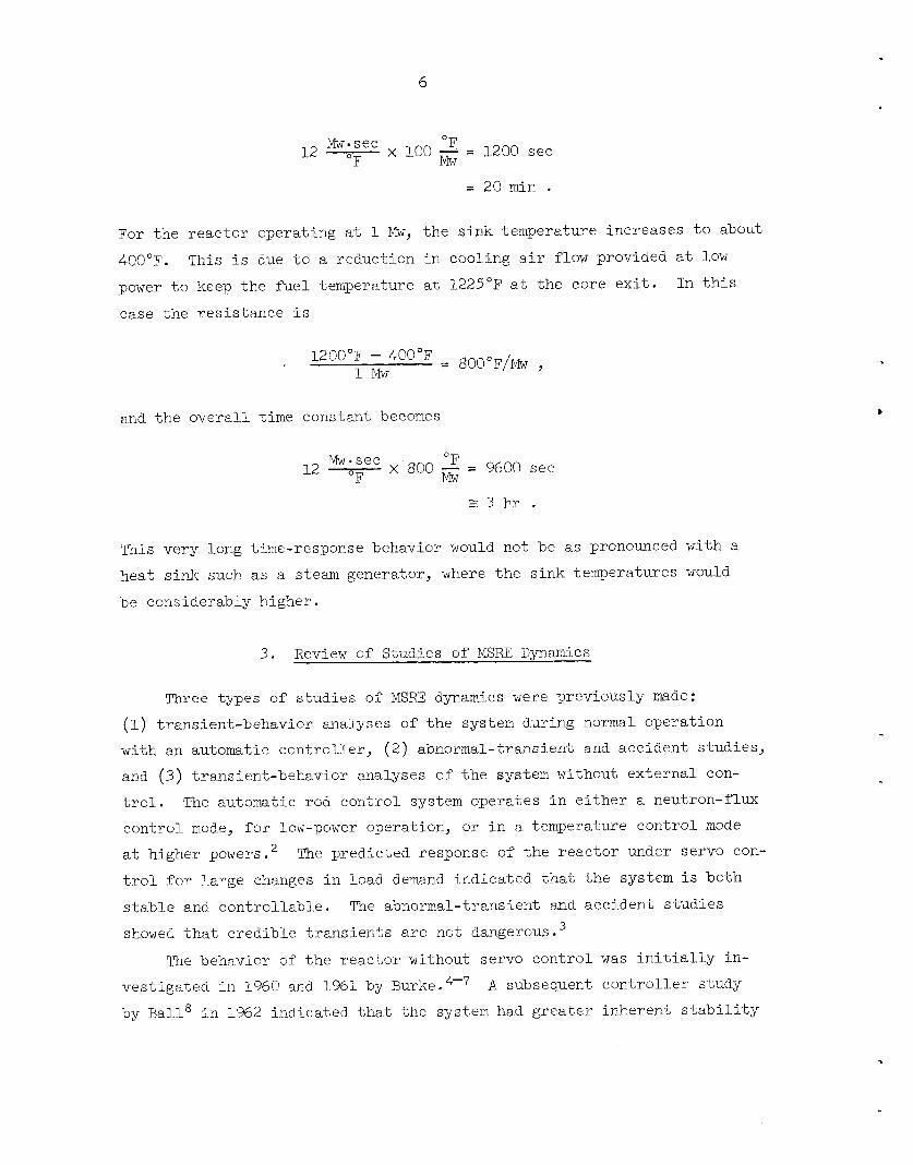
The behavior of the reactor without servo control was initially in-
vestigated in 1960 and 1961 by Burke.4-7 A subsequent controller study
by Ball8 in 1962 indicated that the system had greater inherent stability

7
.
.
than predicted by Burke.
for the two cases.
ferences both in the model and in the parameters used and will be dis-
cussed in detail in Section 6.
Figure 3 shows comparable transient responses The differences in predicted response are due to dif-
There are two important aspects of the MSRE's inherent stability characteristics that were observed in the earlier studies. First, the
reactor tends to become less stable at lower powers, and second, the period of oscillation is very long and increases with lower powers.
shown in Fig. 3, the period is about 9 min at 1 Mw, so any tendency of
the system to oscillate can be easily controlled.
is self-stabilizing at higher powers, it would not tend to run away, or as in this case, creep away. The most objectionable aspect of inherent
oscillations would be their interference with tests planned for the re-
actor without automatic control.
As
Also, since the system
4 . Description of Theoretical Models
Several different models have been used in the dynamic studies of
the MSRE. Also, because the best estimates of parameter values were modi-
fied periodically, each study was based on a different set of parameters.
Since the models and parameters are both important factors in the predic-
tion of stability, their influence on predicted behavior was examined in
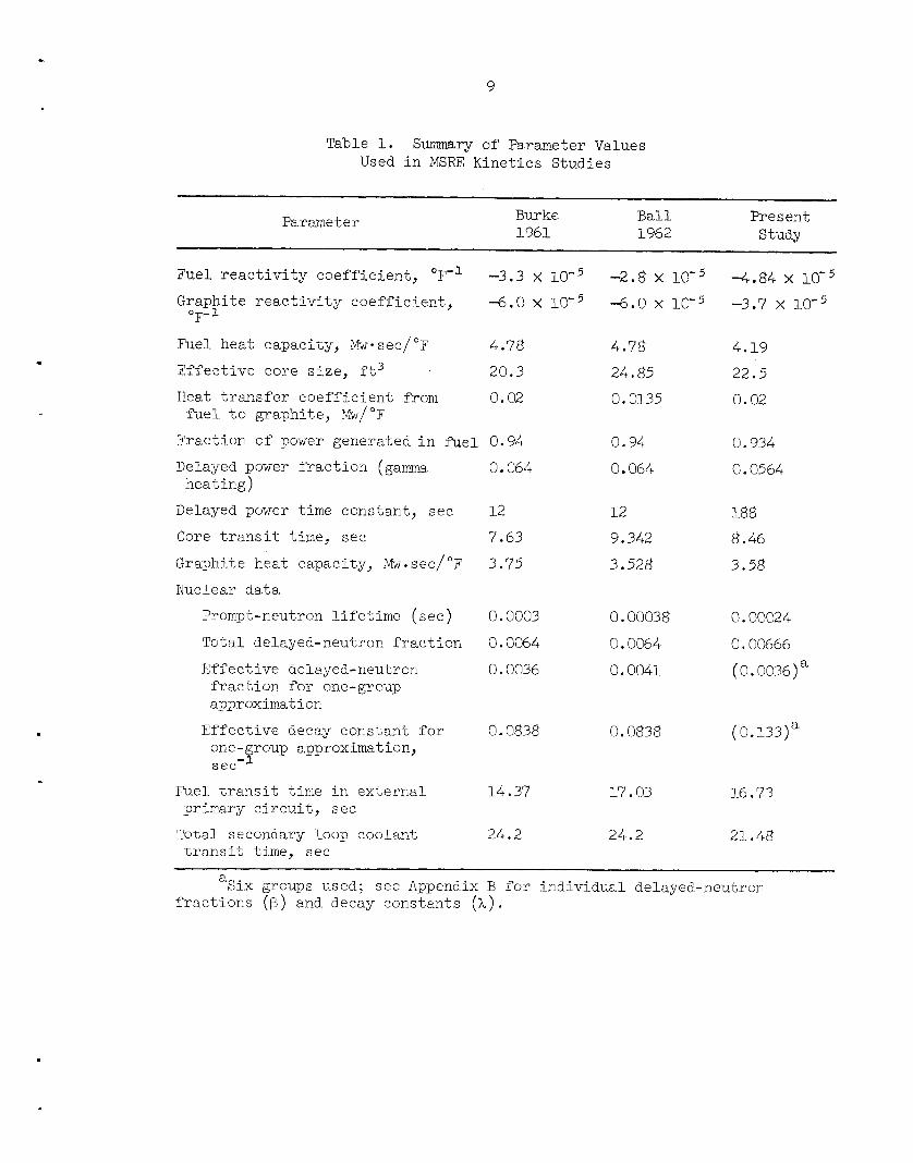
this study. Tables 1, 2, and 3 summarize the various models and parameter
sets used.
Table 2 indicates how each part of the reactor was represented in the three different models, and Table 3 indicates which model was used for
each study. The three models are referred to subsequently as the "Re-
duced, '' "Intermediate, '' and "Complete" models, as designated in Table 2. The models are described in this section, and the equations used are given
in Appendix A. The coefficients for each case are listed in Appendix B.
Table 1 lists the parameters for each of the three studies,
Core Fluid Flow and Heat Transfer
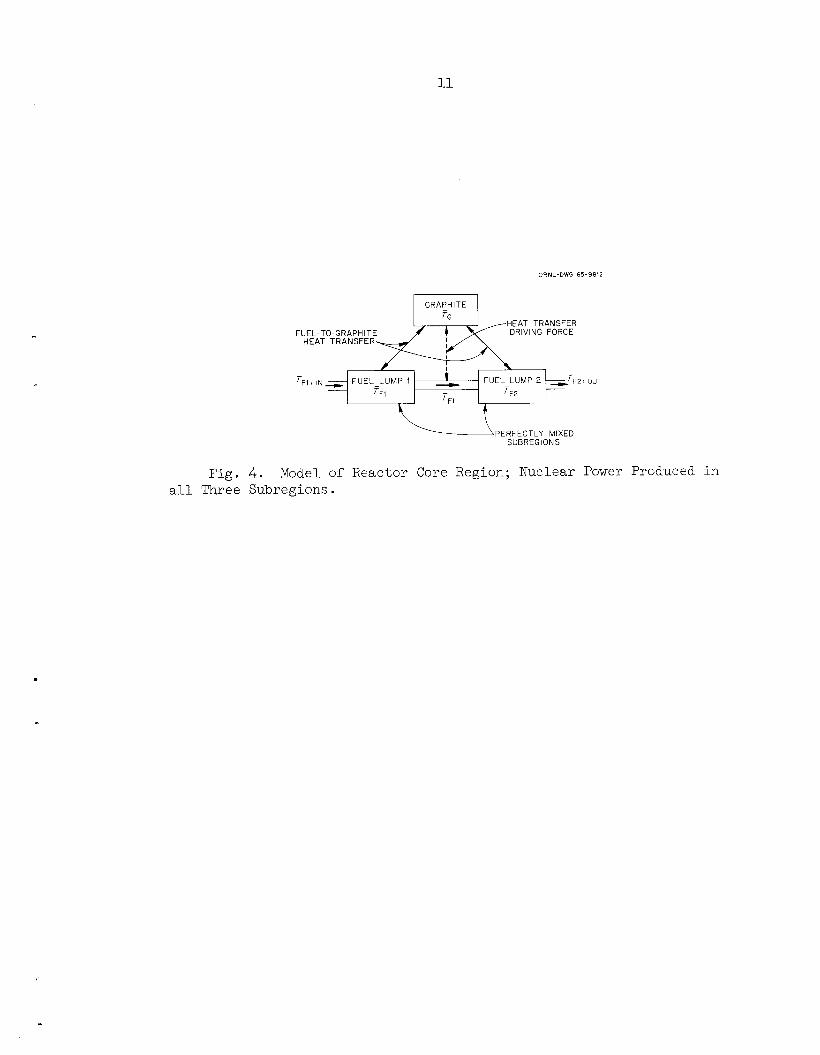
A typical scheme for representing the thermal dynamics of the MSRE core is shown in Fig. 4 . additional explanation. It was desired to base the calculation of heat
The arrows indicating heat transfer require
c
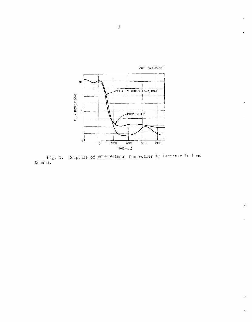
Fig. 3. Demand.
ORNL-DWG 65-9811
1 I I 1
10
c 3 I LL w
v
a 5 X 3 1 LL
200 400 600 800 0 0
TIME (sec)
Response of MSRE Without Controller to De crease in Load
9
.
Table 1. Summary of Parameter Values Used in MSRE Kinetics Studies
Parameter Burke 1961
Ball 1962
Present Study
Fuel reactivity coefficient, "F'l -3.3 x Graphite reactivity coefficient, -6.0 x LO'5 "F- 1
Fuel heat capacity, M w . sec/OF 4.78
Effective core size, ft3 20.3
Heat transfer coefficient from 0.02
Fraction of power generated in fie1 0.94
Delayed power fraction (gamma 0.064
Delayed power time constant, sec 12
Core transit time, see 7.63
Graphite heat capacity, Mw.sec/"F 3.7'5 Nuclear data
fuel to graphite, Mw/"F
heating)
Prompt-neutron lifetime (sec) 0.0003
Total delayed-neutron fraction 0.0064
Effective delayed-neutron 0.0036 fraction for one-group approximation
one-youp approximation, sec-
Effective decay constant for 0.0838
Fuel transit time in external 14.37 primary circuit, sec
transit time, see Total secondary loop coolant 24.2
-2.8 x -6.0 x 10⁻⁵
4.78 24.85 0.0135
0.94
0.064
12
9.342
3.528
0.00038
0.0064
0.0041
0.0838
17.03
24.2
4 . 8 4 x 10⁻⁵ -3.7 x
4.19
22.5 0.02
0.934
0.0564
188 8.46
3.58
0.00024
0.00666
(0.0036) a
(0.133)"
16 .7'3
21.48
a Six groups used; see Appendix B for individual delayed-neutron fractions ( B ) and decay constants (X).
10
Table 2. Description of Models Used in MSRE Kinetics Studies
Reduced Intermediate Complete Model Model Model
Number of core regions 1 9 9
Number of delayed-neutron groups 1 1 6 a Dynamic circulating precursors No No Yes
b Fluid transport lags First Fourth-order Fure order Pad& delay
Fluid-to-pipe heat transfer NO Yes Yes
Number of heat exchanger lumps 1 1 10
Number of radiator lumps 1 1 10
Xenon reactivity No No Yes
In the first two models, the reduced effective delayed-neutron a fraction due to fuel circulation was assumed equal to the steady- state value. explicitly (see Appendix A for details).
order approximation is 1/(1 + 7 s ) . The fourth order Pad6 approxima- tion is the ratio of two fourth-order polynomials in zs, which gives a better approximation of e-"' (see Appendix A).
In the third model, the transient equations were treated
-?S bThe Laplace transform of a time lag, T, is e . The first
Table 3. Models Used in the Various MSRE Kinetics Studies
- .~ ~
Study Model Used
Burke 1961 analog (refs. 4-7) Ball 1962 analog (ref. 8 ) Intermediate
1965 frequency response Complete
1965 transient response Intermediate
1965 extrema determinationa Reduced
1965 eigenvalue calculations Intermediate
1965 frequency response with Comp 1 et e
Reduced
extrema data
The worst possible combination of pa- a rameters was used as described in Section ?.
.
11
7~1, IN = FUEL-LUMP 1 2 FUEL-LUMP 2 ~ - TF2
‘Fl ‘Fl
ORNL-DWG 65-9812
--TF,, OUT -
Fig. 4 . Model of Reactor Core Region; Nuclear Power Produced in a l l Three Subregions.
.
12
transfer rate between the graphite and the fuel stream on the difference
of their average temperatures.
stirred tank" in the fuel stream is taken as the fluid average temperature.
Thus a dotted arrow is shown fromthis point to the graphite to represent
the driving force for heat transfer. However, all the mass of the fluid
is in the lumps, and the heat transferred is distributed equally between
the lumps. Therefore solid arrows are shown from the graphite to each
fluid lump to indicate actual transfer of heat.
The outlet of the first lump or "well-
This model was developed by E. R. Mann* and has distinct advantages over the usual model for representing the fluid by a single lump in which
the following algebraic relationship is used to define the mean fuel tem-
perature :
T inlet + T outlet
2 F F T mean = F
The outlet temperature of the model is given by
T outlet = 2T mean - T inlet . F F F
Since the mean temperature variable represents a substantial heat
capacity (in liquid systems), it does not respond instantaneously to
changes in inlet temperature. Thus a rapid increase in inlet temperature would cause a decrease in outlet temperature - clearly a nonphysical re- sult.
model avoids this difficulty.
With certain limitations on the length of the flow path, g Mann's
The reduced MSRE model used one region to represent the entire core,
and Lhe nuclear average temperatures were taken as the average graphite temperature (r ) and the temperature of the first fuel lump (7 The
nuclear average temperature is defined as the temperature that will give
the reactivity feedback effect when multiplied by the appropriate tem-
perature coefficient of reactivity.
) . G F1
The intermediate and complete models employ the nine-region core
model shown schematically in Fig. 5. Each region contains two fuel lumps
~
Vak Ridge National Laboratory; now deceased.

13
.
UNCLASSIFIED OR NL- DWG 63- 7 319R
1 ‘ I t 4 + -+ 3
2
I
7
-I-
-t 6
5 -+
9
-t 8
i- Fig . 5. Schematic Diagram of Nine-Region Core Model.
and one graphite lump, as shown in Fig. 4. This gives a total of 18 lumps (or nodes) to represent the fuel and nine lumps to represent the graphite.
The nuclear power distribution and nuclear importances f o r all 27 lumps were calculated with the digital code EQUIPOISE-3A, which solves steady- state, two-group, neutron-diffusion equations in two dimensions.
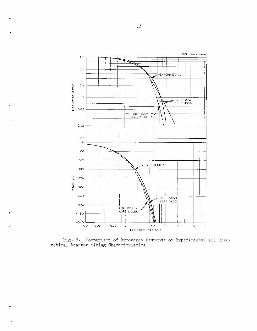
Tests were made on the E R E full-scale core hydraulic mockup'' to
check the validity of the theoretical models of core fluid transport.
salt solution was injected suddenly into the 1200-gpm water stream at the
reactor vessel inlet of the mockup, and the response at the reactor outlet
was measured by a conductivity probe. The frequency response of the sys-
tem was computed from the time response by Samulon's method'' for a sam-
pling rate of 2.5/sec. theoretical models are computed from the transfer function of core outlet-
to-inlet temperature by omitting heat transfer to the graphite and adding
pure delays for the time for fluid transport from the point of salt in-
jection to the core inlet and from the core outlet to the conductivity
probe location. A comparison of the experimental, one-region, and nine- region transfer functions is shown by frequency-response plots in Fig. 6.
Both theoretical curves compare favorably with the experimental curve, especially in the range of frequencies important in the stability study (0.01 to 0.1 radians/sec).
nitude ratios at frequencies as low as 0.1 to 1.0 radians/sec is due to a considerable amount of axial mixing, which is to be expected at the low Reynolds number of the core fluid flow (-1000). This test indicates
that the models used for core fuel. circulation in the stability analyses
are adequate.
A
The equivalent mixing characteristics of the
The relatively large attenuation of the mag-
Neutron Kinetics
The standard one-point, nonlinear, neutron kinetics equations with
one average delayed-neutron group were used in all the analog and digital
transient response studies.
other studies.
values of nuclear importance for each of the 27 lmps were used to compute
the thermal feedback reactivity.
Linearized equations were used for all the
In the studies of a nine-region core model, weighted
Six delayed-neutron groups and the
.
15
ORNL-DWG 65-9813 10
0 5
0 2
01
0 05
0 02
0 01 0
-60
-120
-180
- m ," -240 I
W In 2 -300 a
-360
420
-480
540 5 10 001 002 005 01 02 05 1 2
FREQUENCY (radians/sec)
Fig. 6. Comparison of Frequency Response of Experimental and Theo- retical Reactor Mixing Characteristics.
.

16
dynamic effects of the circulation of the precursors around the primary loop were included in the complete model.
Heat Exchanger and Radiator
The lumping scheme used to represent heat transfer in both the heat
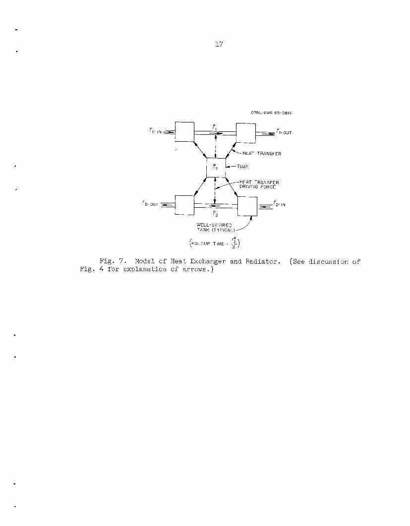
exchanger and the radiator is shown in Fig. 7. two lumps are used to represent each fluid flow path.
intermediate models both used one section as shown. The complete model
used ten of these sections connected sequentially.
As with the core model, The reduced and
Fluid Transport and Heat Transfer in Connecting Piping
The reduced model used single well-stirred-tank approximations for fluid transport in the piping from the core to the heat exchanger, from the heat exchanger to the core, from the heat exchanger to the radiator,
and from the radiator back to the heat exchanger. Since the flow is
highly turbulent (primary system, Re M 240,000; secondary system, Re fi: 120,000), there is relatively little axial mixing, and thus a plug flow model is probably superior to the well-stirred-tank model.
order Pad6 approximations were used in the intermediate model and pure
delays in the complete model (see Appendix A). ing and vessels was also included in the complete model.
Fourth-
Heat transfer to the pip-
Xenon Behavior
The transient poisoning effects of xenon in the core were considered
only in the complete model. The equations include iodine decay into xe- non, xenon decay and burnup, and xenon absorption into the graphite.
*
Delayed Power
In all three models, the delayed-gamma portion of the nuclear power was approximated by a first-order lag.
.
17
- 'T
ORNL-DWG 65-9814
TUBE -
' 2, OUT - - F- F- -T2j F- IN - -
(HOLDUP TIME = 2) 1"
2
Fig. 7. Model of Heat Exchanger and Radiator. (See discussion of Fig. 4 for explanation of arrows. )

18
5. Stability Analysis Results
Data were obtained with the best available estimates of the system
parameters for analysis by the transient-response, closed-loop frequency-
response, open-loop frequency-response, and pole-configuration (root locus) methods.
that (1) comparison of the results provides a means of checking for com-
putational errors; (2) some methods are more useful than others for spe- cific purposes; for example, the pole-configuration analysis gives a clear answer to the question of stability, but frequency-response methods
are needed to determine the physical causes of the calculated behavior;
and (3) certain methods 'are more meaningful to a reader than others, de-
pending on his technical badkground. The differences between the results and earlier resultskm7 are discussed in Section 6, and the effects of
changes in the mathematical model and the system parameters are examined in Section 7.
The advantages in using various analytical methods are
The results show that the MSRE has satisfactory inherent stability
characteristics. Its inherent response to a perturbation at low power
is characterized by a slow return to steady state after a series of low-
frequency oscillations. This undesirable but certainly safe behavior at
l o w power can easily be smoothed out by the control system. 2
Transient Response
The time response of a system to a perturbation is a useful and
easily interpreted measure of dynamic performance. It is not as useful in showing the reasons behind the observed behavior as some of the other methods discussed below, but it has the advantage of being a physically
observable (and therefore familiar) process.
The time response of the reactor power to a step change in k was eff calculated. The IBM-7090 code MATEXP12 was used. MATEXP solves general,
nonlinear, ordinary differential equations of the form
(1) dx dt - = Ax + &(x) x -I- f(t) ,
19
.
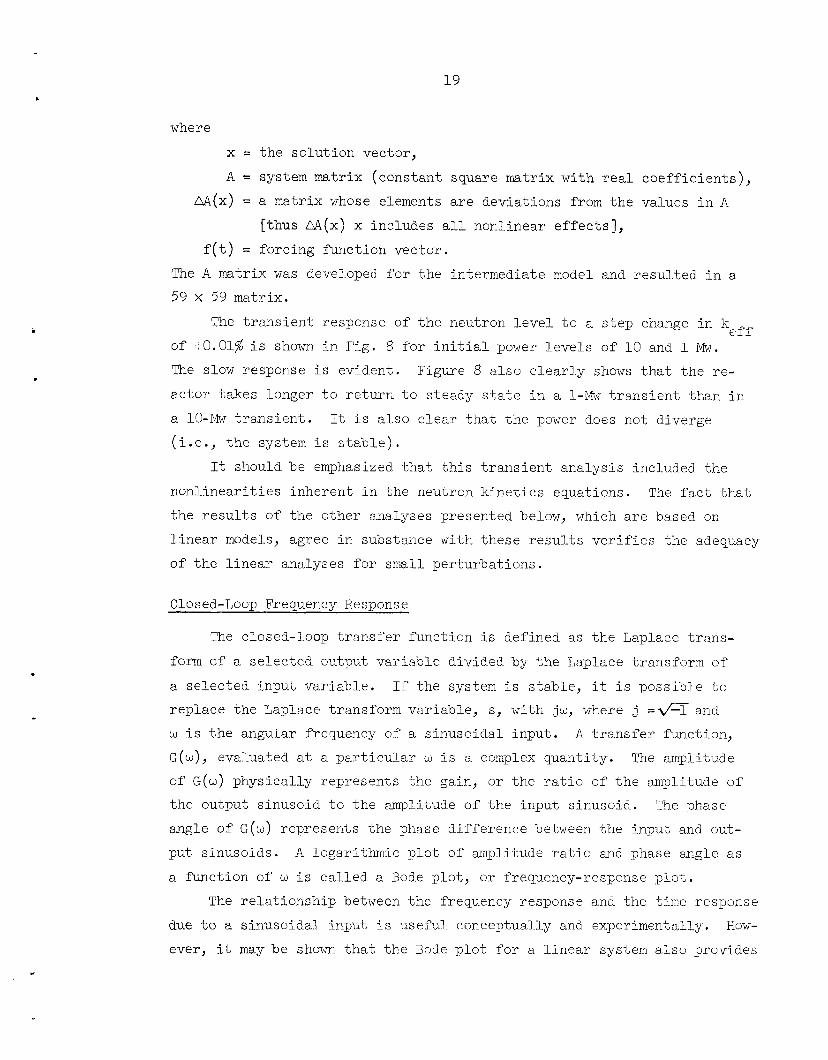
where
x = the solution vector,
A = system matrix (constant square matrix with real coefficients),
U ( x ) = a matrix whose elements are deviations from the values in A [thus M(X) x includes all nonlinear effects],
f(t) = forcing function vector.
The A matrix was developed for the intermediate model and resulted in a 59 x 59 matrix.
eff The transient response of the neutron level to a step change in k
of +0.01$ is shown in Fig. 8 for initial power levels of 10 and 1 Mw. The slow response is evident.
actor takes longer to return to steady state in a 1-Mw transient than in a 10-Mw transient. (i.e., the system is stable).
Figure 8 also clearly shows that the re-
It is also clear that the power does not diverge
It should be emphasized that this transient analysis included the
nonlinearities inherent in the neutron kinetics equations. The fact that
the results of the other analyses presented below, which are based on
linear models, agree in substance with these results verifies the adequacy
of the linear analyses for small perturbations.
Closed-Loop Frequency Response
The closed-loop transfer function is defined as the Laplace trans-
form of a selected output variable divided by the Laplace transform of
a selected input variable. If the system is stable, it is possible to
replace the Laplace transform variable, s , with jw , where j =d-T and w is the angular frequency of a sinusoidal input.
G(w), evaluated at a particular w is a complex quantity. of G ( w ) physically represents the gain, or the ratio of the amplitude of the output sinusoid to the amplitude of the input sinusoid. The phase
angle of G(w) represents the phase difference between the input and out-
put sinusoids. A logarithmic plot of amplitude ratio and phase angle as a function of w is called a Bode plot, or frequency-response plot.
A transfer function, The amplitude
The relationship between the frequency response and the time response
due to a sinusoidal input is useful conceptually and experimentally. How-
ever, it may be shown that the Bode plot for a linear system also provides

20
04
I
3 0 3 5 1 W > w
z 02 0 K + 3 W z
01 W W z I 0
a
$ c
-0
.
Fig. 8. MSRE Transient Response to a -t-o.O1$ 6k Step Reactivity In- put when Operating at 1 and 10 Mw.

21
qualitative stability information that is not restricted to any particu-
lar form in input.13 This information is largely contained in the peaks
in the amplitude ratio curve. High narrow peaks indicate that the system
is less stable than is indicated by lower broader peaks.
The closed-loop frequency response was calculated for N (neutron level fluctuations in megawatts) as a f’unction of 6k (change in input
The MXFR code (a special-purpose code for the MSRE frequency- keff ) . response calculations; see Appendix C) for this calculation. The results for Fig. 9. Fewer phase-angle curves than
to avoid cluttering the plot. Several observations can be based
and the complete model were used
several power levels are shown in
magnitude curves are shown in order
on the information of Fig. 9. First, the peaks of the magnitude curves get taller and sharper with lower
power. This indicates that the system is more oscillatory at low power.
Also the peaks in the low-power curves rise above the no-feedback curve. This indicates that the feedback is regenerative at these power levels.
Also, since the frequency at which the magnitude ratio has a peak approxi- mately corresponds to the frequency at which the system will naturally
oscillate in response to a disturbance, the low-power oscillations are
much lower in frequency than the 10-Mw oscillations.
cillation range from 22 min at 0.1 Mw to 1.3 min at 10 Mw.
The periods of os-
Figure 9 shows that the peak of the 10-Mw magnitude ratio curve is
very broad and indicates that any oscillation would be small and quickly
damped out. The dip in this curve at 0.25 radians/sec is due to the 25- see fie1 circulation time in the primary loop [i.e., (2T radians/cycle)/ (25 sec/cycle) = 0.25 radians/sec] . Here a fuel-temperature perturbation in the core is reinforced by the perturbation generated one cycle earlier that traveled around the loop. Because of the negative fuel-temperature coefficient of reactivity, the power perturbation is attenuated.
?“ne relatively low gains shown at low frequencies can be attributed
to the large change in steady-state core temperatures that would result
from a relatively small change in nuclear power with the radiator air flow rate remaining constant. This means that only a small change in power is required to bring about cancellation of an input 6k perturbation
by a change in the nuclear average temperatures.

22 .
FREQUENCY (radlans/sec)
90
80
7 0
60
50
4 0
3 0
20
0 10 - m - $ 0
2 -10 a
- 2 0
- 3 0
-40
-50
-60
-70
-80
-90 ..
00001 2 5 0001 2 5 0 0 1 2 5 01 2 5 1 2 5 10
FREQUENCY (radians/sec)
Fig. 9. Complete Model Analysis of MSRE Frequency Response for Sev- eral Power Levels.
.

23
.
Open-Loop Frequency Response
A simplified block diagram representation of a reactor as a closed- loop feedback system is shown in Fig. 10. The forward loop, G, represents the nuclear kinetics transfer function with no temperature effects, and the feedback loop, H, represents the temperature (and reactivity) changes due to nuclear power changes.
The closed-loop equation is found by solving for N in terms of 6k:
N = G Gkin - GHN
o r
G 1 +GH
- - - N
The quantity GH is called the open-loop transfer function, and represents the response at point b of Fig. 10 if the loop is broken at point b. Equation (2) shows that the denominator of the closed-loop transfer func- tion vanishes if GH = -1. Also, according to the Nyquist stability cri-
terion, the system is unstable if the phase of GH is more negative than -180" when the magnitude ratio is unity. loop frequency response contains information about system dynamics that
are important in stability analyses.
Thus it is clear that the open-
A useful measure of system stability is the phase margin. It is de-
fined as the difference between 180" and the open-loop phase angle when the gain is 1.0.
found in suitable references on servomechanism theory.13
cation, it suffices to note that smaller phase margins indicate reduced stability. a phase margin of at least 30" is desirable. indicate lightly damped oscillation and poor control.
dicates an oscillating system, and negative phase margins indicate insta-
bility.
A discussion of the phase margin and its uses may be For this appli-
A general rule of thumb in automatic control practice is that Phase margins less than 20"
Zero degrees in-
The phase margin as a fbnction of reactor power level is shown in
Fig. 11. 30' at about 0.5 Mw.
at 0.1 Mw.
The phase margin decreases as the power decreases and goes below
However, the phase margin is still positive (12")
These small phase margins at low power suggest slowly damped

24
ORNL-DWG 65-9817
FORWARD LOOP Sk N E T Y ) /
B R E A K LOOP HERE skinIf 1 T F : R POWER, Mw
FOR OPEN-LOOP ANALYSI S-b
ak F E E D B A C K \ I \ FEEDBACK LOOP
Fig. 10. Reactor as a Closed-Loop Feedback System.
100 ORNL-DWG 65-9818
50
2 0
10
5
2
1 0 0 5 01 0 2 0 5 1 2 5 10 20
No, NUCLEAR POWER (Mw)
*
Fig. 11. Period of Oscillation and Phase Margin Versus Power Level for MSFR Calculation with Complete Model.

25
oscillations, as has been observed in the transient-response and closed- loop frequency-response results.
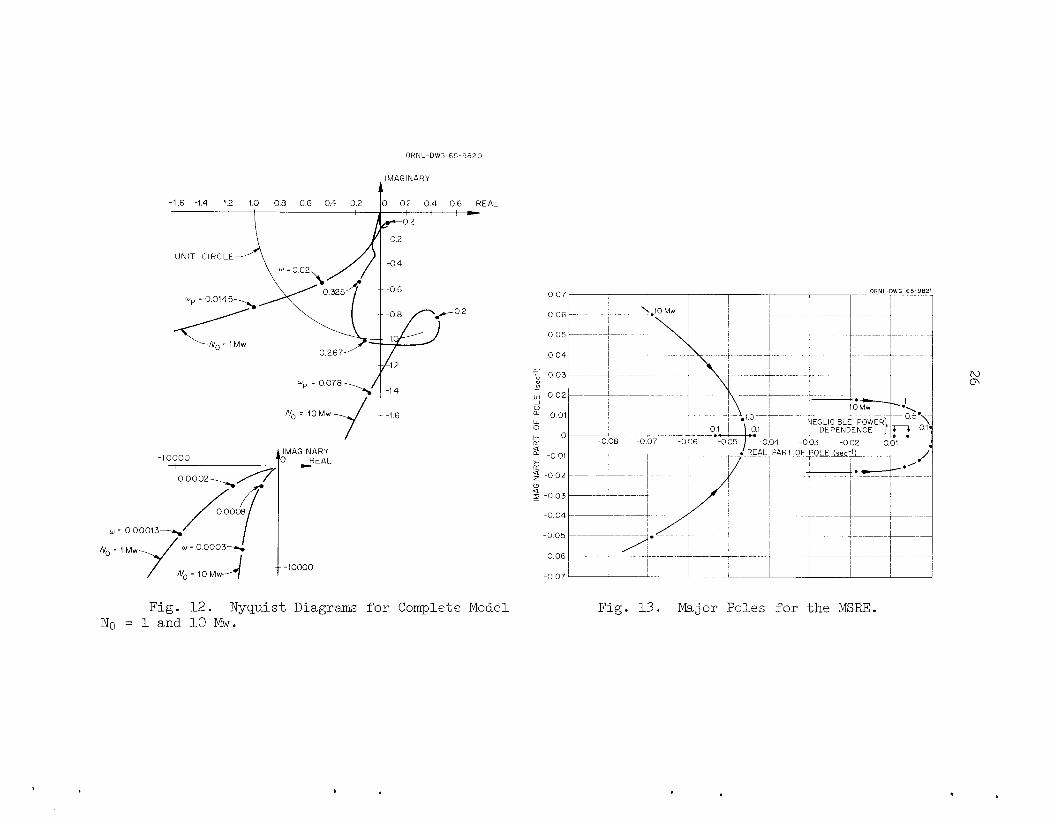
of power level is also shown in Fig. 11. Figure 12 shows Nyquist plots for the open-loop transfer function,
It is clear that the unstable condition of
The period of oscillation as a function
GH, at 1.0 Mw and 10.0 Mw.
(lGHl = 1 and phase angle -180") is avoided. In order for the phase mar- gin to be a reliable indication of stability, the Nyquist plot must be "well-mannered" inside the unit circle; that is, it should not approach the critical (-1.0 +jO) point.
have peculiarly in approaching the origin, they do not get close to the
critical point.
Although the curves shown in Fig. 12 be-
Pole Configuration
The denominator (1 + GH) of the closed-loop transfer function of a lumped-parameter system is a polynomial in the Laplace transform variable, s . are the poles of the system transfer function.
the eigenvalues of the system matrix A in Eq. (1). ficient condition for linear stability is that the poles all have nega-
tive real parts.
the complex plane and the dependence of their location on power level.
The roots of this polynomial (called the characteristic polynomial)
The poles are equal to
A necessary and suf-
Thus, it is useful to know the location of the poles in
The poles were calculated for the intermediate model of the MSRE (see Section 4 ) .
59 X 59 matrix used in the transient analysis. The calculations were performed with a modification of the general matrix eigenvalue code Q3l4 for the IBM-7090. The results are shown in Fig. 13 for several of the major poles. It is clear from Fig. 13 that the system is stable at all power levels. The set of complex poles that goes to zero as the power decreases is the set primarily responsible for the calculated dynamic performance.
imaginary part of this set approximately represents the natural frequency
of oscillation of the system following a disturbance.
oscillation decreases as the power decreases, as observed previously.
The matrix used was the linearized version of the
A l l the other poles lie far to the left of the ones shown.
The
The frequency- of
26
N 0 I
27
6. Interpretation of Results
Explanation of the Inherent Stability Characteristics
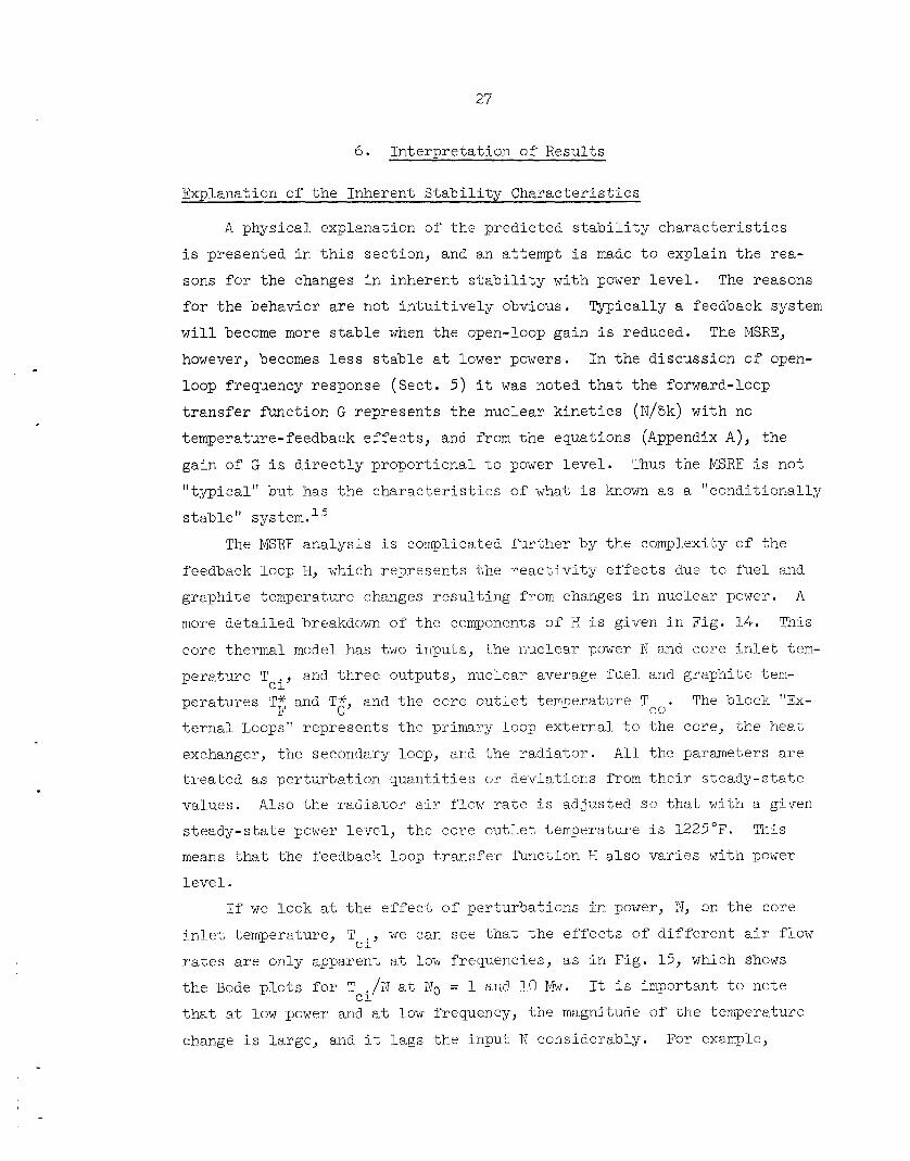
A physical explanation of the predicted stability characteristics is presented in this section, and an attempt is made to explain the rea-
sons for the changes in inherent stability with power level. The reasons
for the behavior are not intuitively obvious. Typically a feedback system
will become more stable when the open-loop gain is reduced. The MSRE,
however, becomes less stable at lower powers. In the discussion of open- loop frequency response (Sect. 5 ) it was noted that the forward-loop transfer function G represents the nuclear kinetics (N/6k) with no temperature-feedback effects, and from the equations (Appendix A), the
gain of G is directly proportional to power level. "typical" but has the characteristics of what is known as a "conditionally
stable ' I system.
Thus the MSRE is not
The MSRE analysis is complicated further by the complexity of the
feedback loop H, which represents the reactivity effects due to fuel and graphite temperature changes resulting from changes in nuclear power. A more detailed breakdown of the components of H is given in Fig. 14. core thermal model has two inputs, the nuclear power N and core inlet tem- perature Tci, and three outputs, nuclear average fuel and graphite tem- peratures T* and T*, and the core outlet temperature Tco.
ternal Loops" represents the primary loop external to the core, the heat
exchanger, the secondary loop, and the radiator. All the parameters are treated as perturbation quantities or deviations from their steady-state values. Also the radiator air flow rate is adjusted SO that with a given
steady-state power level, the core outlet temperature is 1225°F. This
means that the feedback loop transfer f'unction H also varies with power level.
This
The block "Ex- F G
If we look at the effect of perturbations i.n power, N, on the core inlet temperature, Tci, we can see that the effects of different air flow rates are only apparent at low frequencies, as in Fig. 15, which Bhows the Bode plots fo r T ./N at No = 1 and 10 Mw. It is important to note that at low power and at low frequency, the magnitude of the temperature
change is large, and it lags the input N considerably.
e1
For example,

N
N
m ? w
0
0
J
z
n
0
W z
-%
M
16
-%
M
d 0
a, .rl
29
at No = 1 Mw and w = 0.0005 radians/sec, the magnitude ratio is 170°F/Mw and the phase lag is 80". The block diagram of Fig. 14 indicates that the nuclear average temperature perturbations in T* and T* can be con- F G sidered to be caused by the two separate inputs N and Tci.
the open-loop transfer function T*/N (with Tci constant) is 5.0"F/Mw at
steady state, and there is little attenuation and phase lag up to rela- tively high frequencies, as in Fig. 16, which shows the open-loop transfer
functions of the nuclear average temperatures as functions of N and T . Returning to the example case of No = 1 Mw and w = 0.0005 radians/sec, we note that the prompt feedback effect of 5"F/Mw from T$/N is very small
compared with temperature changes of the entire system represented by a
For example,
F
ci
T ./N of 170"F/Mw at -80". (Note that Tg/Tci = 1.0 at 0.0005 radians/sec.) c 1 The important point here is that for low power levels over a wide range
of low frequencies, the large gain of the frequency response of overall system temperature relative to power dominates the feedback loop H, and its phase angle approaches -90".
The no-feedback curve in Fig. 9 shows that at frequencies below about
0.005 radians/sec, the forward-loop transfer function N/6k (open loop)
also has a phase approaching -90" and a gain curve with a -1 slope (i.e.,
one-decade attenuation per decade increase in frequency). and H having phase angles approaching -90°, the phase of the product GH will approach -180". under these conditions, the system would approach instability. From the
Bode plot of Fig. 9, it can be seen that at a power of 0.1 Mw, I GH I x 1.0 at 0.0045 radians/sec (22 min/cycle), since the peak in the closed-loop
occurs there. At lower powers and consequently lower gains G, IGH I ap- proaches 1.0 at even lower frequencies, where the phase of GH is closer to -180". This accounts for the l e s s stable conditions at the lower powers and lower frequencies.
With both G
If the magnitude ratio of G were such that lGHl = 1.0
At the higher powers, lGHl approaches 1.0 at higher frequencies where the effect of the prompt thermal feedback is significant. For ex-
ample, the peak in the 10-Mw closed-loop Bode plot of N/6k, Fig. 9, occurs
at 0.078 radians/sec. (Fig. 15) compared with a T*/N of 4.4 at -15" (Fig. 16).
the prompt fuel temperature feedback term has a dominant stabilizing effect.
At this frequency, I Tci/N I has a value of 2.0 Consequently, F

30
0
- 1 5
- 3 0
-45 - Cm $ -60 W m 2 -75 Q
-90
-105
-120
O H N L - D W G 65-9824
Fig. 16. Open-Loop Frequency-Response Diagrams of Nuclear Average Temperatures as Functions of Nuclear Power and Core Inlet Temperature.

31
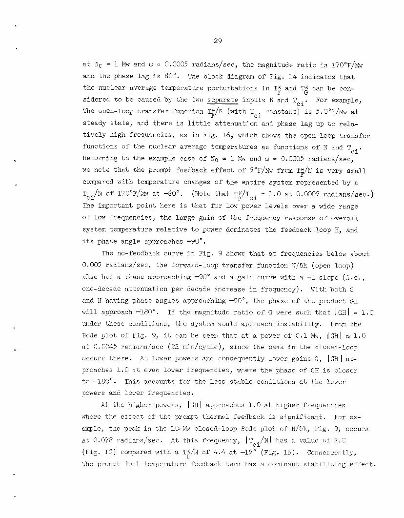
6k prompt N - - - F
in 6k aF ( 8k/ O F 1 TFx - closed loop open loop
and
The net 6k vector is the sum of the input and feedback vectors. For the 1-Mw case, 6k net is greater than 6k - this indicates regenerative feed- back and shows up on the closed-loop Bode plot (Fig. 9) as a peak with a greater magnitude ratio than that of the no-feedback curve.
in'
The increased stabilizing effect of the prompt fuel temperature term
in going from 1 to 10 Mw is also evident. diminished effect of the graphite at the higher frequency.
These plots clearly show the
In both cases, too, the plots show that a more negative graphite
temperature coefficient would tend to increase the net 6k vector and hence destabilize the system.
Interpretation of Early Results
The previously published results of a dynamic study performed in 1961 predicted that the MXRE would be less stable than is predicted in this study. This is partly because of differences in design parameters
and partly because of differences in the models used. These differences
were reviewed in Section 4 of this report.
32
ORNL-DWG 65-9825
-6k, * : i k F LOOP -6kG TOTAL PROMPT
A6k NET
Po = 1Mw
= 0 0145 RADIANWSEC
- 6 k F PROMPT
3 t B k , "
Fig . 17. Directed-Line Diagrams of Reac t iv i ty Feedback E f f e c t s a t 1 and 10 Mw f o r Complete Model.

33
The most significant parameter changes from 1961 to 1965 were the values for the fuel and graphite temperature coefficients of reactivity
and the changes in the fuel heat capacity.
the new fuel coefficient is more negative, the new graphite coefficient
is less negative, and the fuel heat capacity is smaller than was thought
to be the case in 1961. A l l these changes contribute to the more stable
behavior calculated with the current data. (The destabilizing effect of a more negative graphite temperature coefficient is discussed in Section
Table 1 (Sect. 4 ) shows that
7. ) The most important change, however, is the use of a multiregion core
model and the calculation of the nuclear average temperature.
single-region core, T* is equal to the temperature of the first of the
two fuel lumps or the average core temperature (in steady state), In
the nine-region core, T* is computed by multiplying each of the 18 fuel- lump temperatures by a nuclear importance factor, I. region model, the steady-state value of T*/N (with Tci constant) is only
2.8'F/Mw compared with 5.0°F/Mw for the nine-region core model. difference occurs because in the nine-region model, the downstream fuel-
lump temperatures are affected not only by the power input to that lump
but also by the change in the lump's inlet temperature due to heating of
the upstream lumps. This point may be illustrated by noting the differ-
ence between two single-region models, where in one case the nuclear im-
portance of the first lump is 1.0 and in the other case the importance
of each lump is 0.5. As an example, say the core outlet temperature in- creases 5"F/Mw.
In the
F
F In the single-
F This
The change in T* for a 1-Mw input would be F
In the first case 11 = 1.0 and AT1 = 2.5"F, so AT; = 23°F. In the sec-
ond case, 11 = I2 = 0.5, AT1 = 2.5"F, and AT2 = 5"F, so AT* = 3.75"F, or F a 50% greater change than in case one. For many more lumps, this effect
is even greater. A s was shown above, the prompt fuel reactivity feedback effect was
the dominant stabilizing mechanism at both 1 and 10 Mw, so the original
single-region core model would give pessimistic results.
34
7 . Perturbations in the Model and the Design Parameters
Every mathematical analysis of a physical system is subject to some
uncertainty because of two questions:
and how accurate are the values of the parameters used in the model?
influence of changes in the assumed model were therefore investigated,
and the sensitivity to parameter variations of the results based on both
the reduced and complete models was determined. An analysis was also
performed to determine the worst expected stability performance within
the estimated range of uncertainty of the system parameters.
How good is the mathematical model, The
Effects of Model Changes
The effects of changing the mathematical model of the system were
determined by comparing the phase margins with the reference case as
each part of the model was changed in turn. The following changes were
made :
1. Core Representation. A single-region core model was used in- stead of the nine-region core used in the complete model.
2. Delayed-Neutron Groups. A single delayed-neutron group was
used instead of the six-group representation in the complete model.
3. Fixed Effective B ' s . The usual constant-delay-fraction delayed-
neutron equations were used with an effective delay fraction, B, for each precursor. The effective p was obtained by calculating the delayed-
neutron contribution that is reduced due to fluid flow in the steady- state case. This i s in contrast to the explicit treatment of dynamic circulation effects in the complete model (see Appendix A).
4 . First-Order Transport Lags. The Laplace transform of a pure -TS delay, e , was used in the complete model. The first-order well- ' was used in the modified model. 1 t- 7s' stirred-tank approximation,
5. Single-Section Heat Exchanger and Radiator. A single section was used to represent the heat exchanger and radiator rather than the
ten-section representation in the complete model. 6. Xenon. The xenon equations were omitted in contrast to the ex-
plicit xenon treatment in the complete model.
35
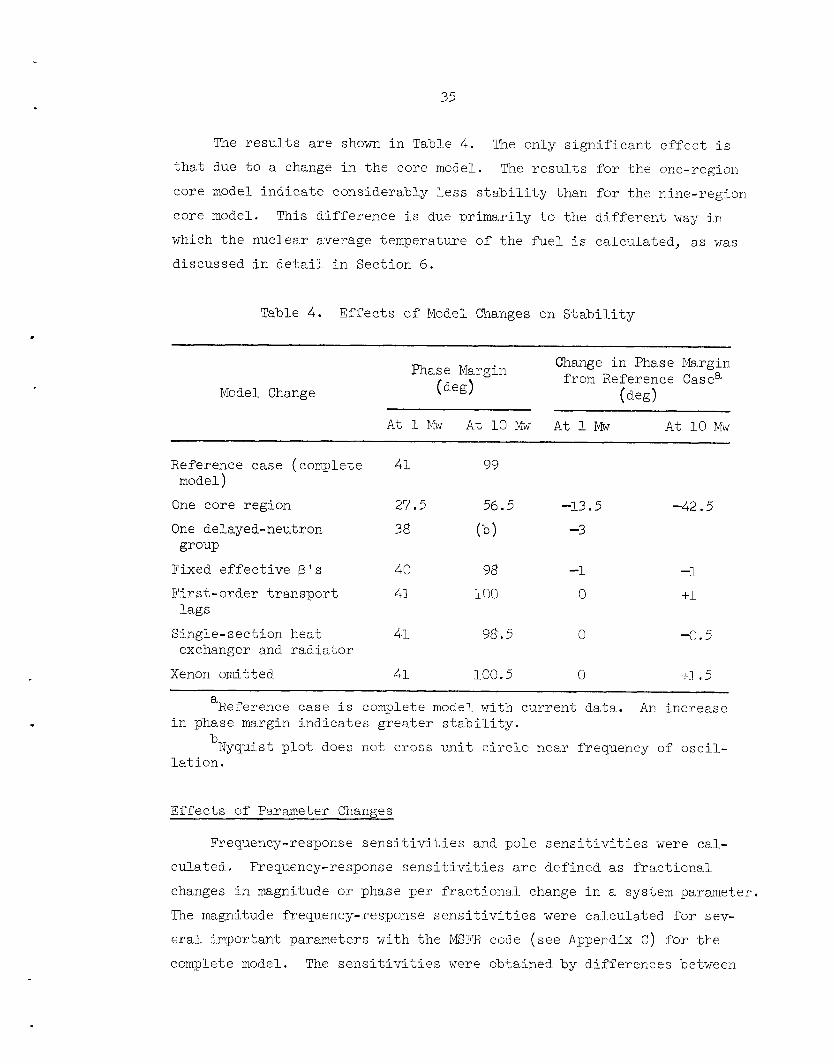
The results are shown in Table 4 . The only significant effect is that due to a change in the core model. The results for the one-region core model indicate considerably less stability than for the nine-region
core model. This difference is due primarily to the different way in
which the nuclear average temperature of the fuel is calculated, as was
discussed in detail in Section 6.
Table 4 . Effects of Model Changes on Stability
Change in Phase Margin from Reference Case" Phase Margin
( d - 4 Model Change (deg)
At 1 Mw At 10 Mw At 1 Mw At 10 Mw
Reference case (complete 41 99 model)
One core region 27.5 56.5 -13.5 -42.5 One delayed-neutron 38 (b ) -3
Fixed effective B ' s 40 98 -1 group
First-order transport 41 100 0 lags
-1 +1
Single-section heat 41 98.5 0 -0.5 exchanger and radiator
Xenon omitted 41 100.5 0 +1.5
'Reference case is complete model with current data. An increase in phase margin indicates greater stability.
bNyquist plot does not cross unit circle near frequency of oscil- lation.
Effects of Parameter Changes
Frequency-response sensitivities and pole sensitivities were cal-
culated. Frequency-response sensitivities are defined as fractional
changes in magnitude or phase per fractional change in a system parameter.
The magnitude frequency-response sensitivities were calculated for sev-
e r a l important parameters with the MXFR code (see Appendix C) for the complete model. The sensitivities were obtained by differences between
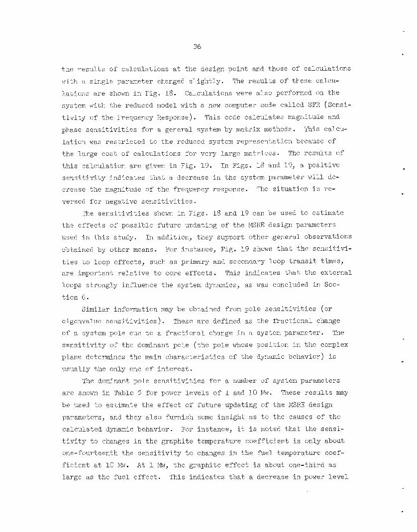
36
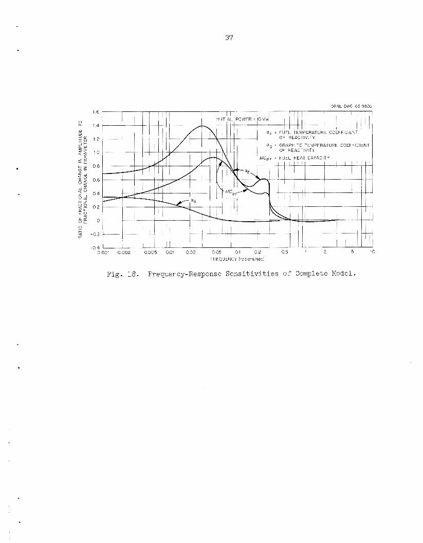
the results of calculations at the design point and those of calculations
with a single parameter changed slightly. The results of these calcu-
lations are shown in Fig. 18. Calculations were also performed on the
system with the reduced model with a new computer code called SFR (Sensi-
tivity of the Frequency Response).
phase sensitivities for a general system by matrix methods.
lation was restricted to the reduced system representation because of the large cost of calculations for very large matrices.
this calculation are given in Fig. 19. In Figs. 18 and 19, a positive sensitivity indicates that a decrease in the system parameter will de- crease the magnitude of the frequency response.
versed for negative sensitivities.
This code calculates magnitude and
This calcu-
The results of
The situation is re-
The sensitivities shown in Figs. 18 and 19 can be used to estimate the effects of possible future updating of the MSRE design parameters
used in this study. In addition, they support other general observations
obtained by other means. For instance, Fig. 19 shows that the sensitivi- ties to loop effects, such as primary and secondary loop transit times, are important relative to core effects. This indicates that the external
loops strongly influence the system dynamics, as was concluded in Sec-
tion 6. Similar information may be obtained from pole sensitivities (or
eigenvalue sensitivities).
of a system pole due to a fractional change in a system parameter. The
sensitivity of the dominant pole (the pole whose position in the complex
plane determines the main characteristics of the dynamic behavior) is usually the only one of interest.
These are defined as the fractional change
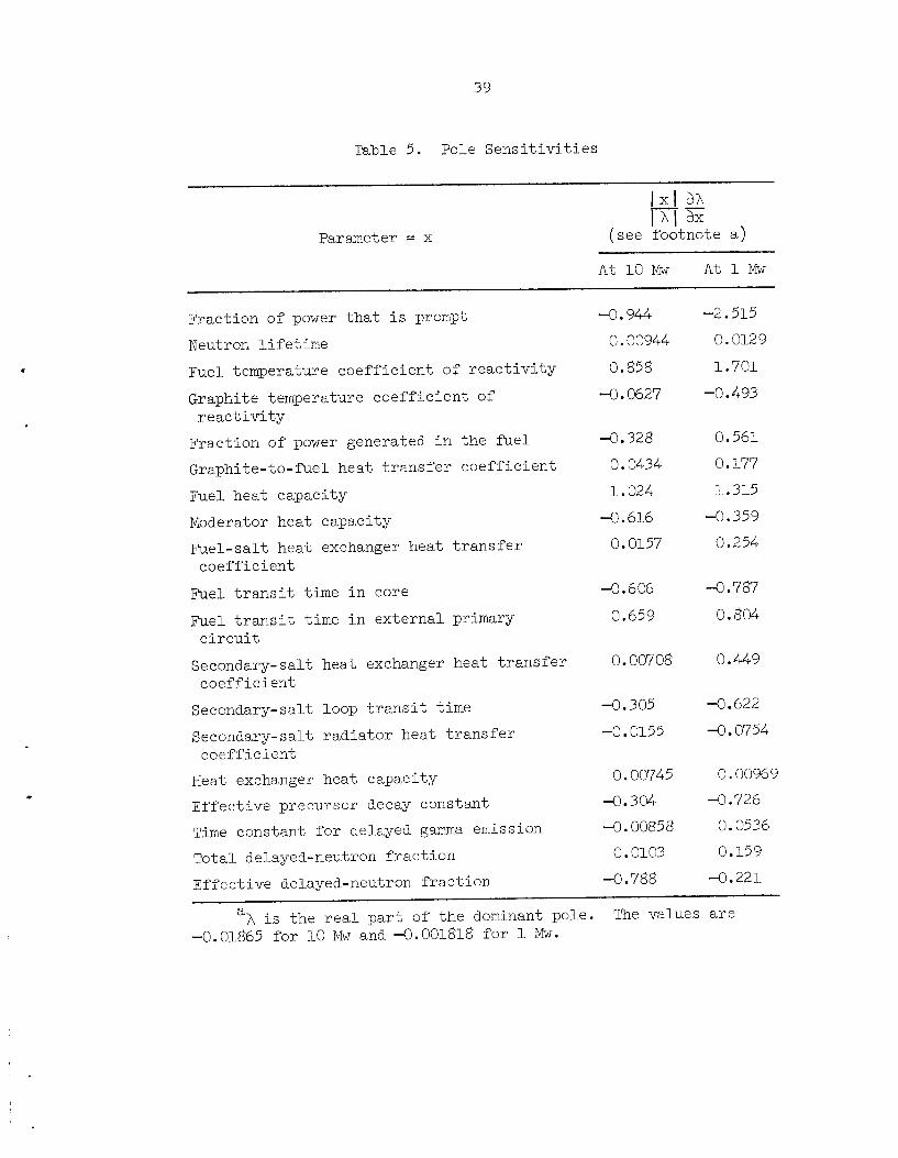
The dominant pole sensitivities for a number of system parameters
are shown in Table 5 for power levels of 1 and 10 Mw. These results may
be used to estimate the effect of future updating of the MSRE design
parameters, and they also furnish some insight as to the causes of the
calculated dynamic behavior. For instance, it is noted that the sensi-
tivity to changes in the graphite temperature coefficient is only about one-fourteenth the sensitivity to changes in the f’uel temperature coef-
ficient at 10 Mw. At 1 Mw, the graphite effect is about one-third as
large as the fuel effect. This indicates that a decrease in power level
37
.
0 c
O a + LL
ORNL-DWG 65 9826 1 6
1 4
1 2 aG = GRAPHITE TEMPERATURE COEFFICIENT
OF REACTIVITY 10
08
0 6
0 4
0 2
0
-0 2
0 5 1 2 5 10 -0 4
0001 0002 0005 001 002 005 01 0 2
FREQUENCY (radions/sec)
Fig. 18. Frequency-Response Sensitivities of Complete Model.

38
0 -
1 5
1.0
0 5
A n
TRANSFER COEFFICIENT , , ~, - +i;: -_ -
o s I W
n = K 0 -
<: - 0 5 GRAPHITE TEMPERATURE COEFFICIENT
k k
0 5 I I , I I ,
1 1 I 0
< FRACTION OF POWER
/
F O , I , , '
GENERATED, IN, T,HE FUEL - - 0 5
O 5 I G R A ~ H I ~ E - T ~ Y U ~ L HEAT ~ i I I I I I I 1 1
0001 2 5 0.01 2 5 01 2 FREQUENCY ( rad lanskec )
ORNL-DWG 65-9827 0 5
0
-0 5 0 5
0
-0 5 0 5
0
-0 5 0
- 0 5
- 1 0
-
16
0 5
0
-0 5 0 5
0
-05 0 5
0
-0 5
___
EXC,HANGER ,H,EAT TRA,NSFER C,OEFFICIEN,T
SPECIFIC HEAT OF SECONDARY SALT
0001 2 5 001 2 5 01 2
FREQUENCY ( rad ianskec)
Fig. 19. Frequency-Response Sensitivities of Reduced Model at a Power of 10 Mw Based on Current Data.
39
Table 5. Pole Sensitivities
.
-- 1x1 ah l h l ax
Parameter = x (see footnote a)
At 10 Mw At 1 Mw
Fraction of power that is prompt
Neutron lifetime
Fuel temperature coefficient of reactivity
Graphite temperature coefficient of
Fraction of power generated in the fie1 Graphite-to-fuel heat transfer coefficient
Fuel heat capacity
Moderator heat capacity Fuel-salt heat exchanger heat transfer
Fuel transit time in core Fuel transit time in external primary
Secondary-salt heat exchanger heat transfer
Secondary-salt loop transit time
Secondary-salt radiator heat transfer
Heat exchanger heat capacity Effective precursor decay constant Time constant for delayed gamma emission Total delayed-neutron fraction Effective delayed-neutron fraction
reactivity
coefficient
circuit
coefficient
coefficient
-0.944
0.00944
0.858
-0.0627
-0.328 0.0434
1.024
-0.616
0.0157
-0.606
0.659
O.OWO8
-0.305
-0.0155
0.00745
-0.304
-0.00858
0.0103
-0.788
-2.515 0.0129
1.701
-0.493
0.561
0.177
1.315
-0.359
0.254
-0.787 0.804
0.449
-2.622
-0.0754
0.00969
-0.726 0.0536
0.159
-0.221
a A is the real part of the dominant pole. The values are -0.01865 for 10 Mw and -0.001818 for 1 Mw.
,
40
causes modifications in the dynamic behavior that accentuate the relative
effect of graphite temperature feedback. It is also noted that the vari- ous heat transfer coefficients have a much larger relative effect at 1 Mw
than at 10 Mw; this indicates that the coupling between system components
has a larger influence at low power than at high power.
Effects of Design Uncertainties
A new rnethodl6 for automatically finding the least stable condition in the range of uncertainty in the design parameters was used. A com- puter code for the IBM-7090 was used for the calculations. The method is described in some deta-il in Appendix D. The least stable condition
is found by using the steepest-ascent (or gradient-projection) method of nonlinear programming.
The quantity that is maximized is the real part of the dominant pole
of the system transfer function (or equivalently, the dominant eigenvalue
of the system matrix).
negative values for the real part of the dominant pole, and instability
is accompanied by a pole with a positive real part.
involves a step-wise determination of the particular combination of sys-
tem parameters within the uncertainty range that causes the real part of
the dominant pole to have its least negative value. If the maximized pole has a negative real part, instability is not possible in the uncer-
tainty range. If the maximized pole has a positive real part, instability is possible in the uncertainty range if all the system parameters deviate
from the design point in a particular way.
Less stable conditions are accompanied by less
The maximization
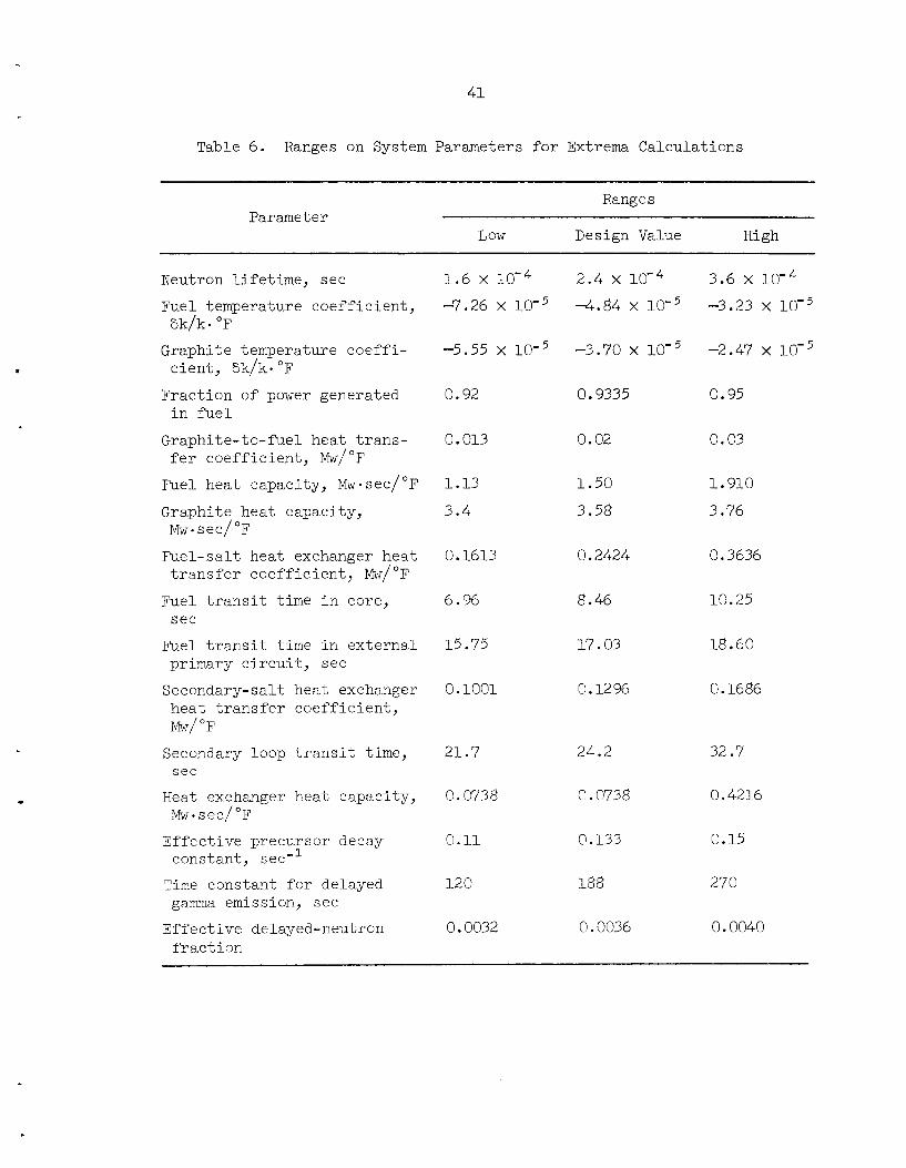
A key factor in the stability extrema analysis is the availability of the appropriate ranges to assign to the system parameters. The ranges
appropriate for the MSRE were furnished by Engel.17 It was decided to use a wide range on the important nuclear parameters (neutron lifetime,
fuel temperature coefficient of reactivity, and graphite temperature co-
efficient of reactivity).
two-thirds and three-halves of the design values.
assigned by considering the method of evaluating them and the probable
effects of aging in the reactor environment. The ranges of the 16 system
parameters chosen for this study are given in Table 6.
These parameters were allowed to range between
All other ranges were
41
Table 6. Ranges on System Parameters for Extrema Calculations
Ranges
Low Design Value High Parameter
1.6 x -7.26 x
2.4 x 4.84 x
3.6 x -3.23 x 10'~
Neutron lifetime, sec Fuel temperature coefficient,
Graphite temperature coeffi-
Fraction of power generated
Graphite-to-fuel heat trans-
Fuel heat capacity, Mw. sec/'F
Gr ap hi t e he at c apa c i t y , Mw. see/ OF
Fuel-salt heat exchanger heat transfer coefficient, MW/'F Fuel transit time in core, see Fuel transit time in external primary circuit, sec
heat transfer coefficient,
Secondary loop transit time,
Heat exchanger heat capacity,
Effective precursor decay
Time constant for delayed
Effective delayed-neutron
6k/k* OF
cient, 6k/k. "F
in fuel
fer coefficient, M~/"F
Secondary-salt heat exchanger
Mw/ "F
s e e
Mw. sec/"F
constant, sec-l
gamma emission, sec
fraction
-5.55 x -3 .yo x 10- -2.47 x
0.92 0.9335 0.95
0.013 0.02 0.03
1.13
3.4 1.50
3.58
1.910
3.76
0.2424 0.1613 0.3636
6.96
15.75
0.1001
8.46 10.25
17.03 18.60
0.1296 0.1686
21.7
0.0738
0.11
120
0.0032
24.2
0.0738
0.133
188
0.0036
32.7
0.4216
0.15
27 0
0.0040
42
The reduced model was used with current parameters for locating the
least stable condition in the uncertainty range. This gave results at
a much lower cost than with a more complete model. This was considered
adequate because other calculations showed that the reduced model predicts
lower stability than the complete model. The reasons for this were ex-
plored in Section 6. Experience with other calculations also showed that
changes in system parameters gave qualitatively the same type of changes
in the system performance with either model.
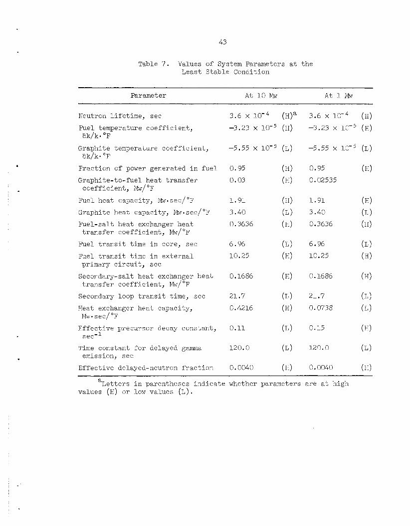
The set of parameters for the least stable condition is listed in
Table '7. The least negative value of the dominant eigenvalue calculated with the reduced model changes from (-0.0187 i. 0.0474 j) sec-l at the de- sign point to (-0.00460 ? 0.0330 j) see-' at the worst condition for 10
Mw. (+0.0005'74 F 0.0134 j) see-'. This indicates that instability is im-
possible in the uncertainty range at 10 Mw but that the reduced model
predicts an instability at 1 Mw for a combination of parameters within
the uncertainty range. This condition gives a transient with a doubling time of about 1/2 hr and a period of oscillation of about 8 min per cycle.
For 1 Mw, the change is from (-0.00182 2 0.0153 j) sec-l to
It is evident that the calculated instability at the extreme case
for 1 Mw is due to the inherent pessimism of the reduced model (see Sect.
6). This was verified by using the MSFR code for the complete model with the parameters describing the extreme case. It was found that the phase margin for 10 Mw was 75" for the extreme condition (versus 99" for the
design condition), and the phase margin f o r 1 Mw was 21" €or the extreme
condition (versus 41" for the design condition). that the best available methods indicate that the MSRE will be stable throughout the expected range of system parameters.
Thus, it is concluded
8. Conclusions
.
This study indicates that the MSRE will be inherently stable for all
operating conditions. Low-power transients without control will persist
for a long time, but they will eventually die out because of inherent feedback. Other studies have shown that this sluggish response at low
43
Table 7. Values of System Parameters at the Least Stable Condition
8
Parameter At 10 Mw At 1 Mw
Neutron lifetime, see
Fuel temperature coefficient,
Graphite temperature coefficient,
Fraction of power generated in fuel Graphite-to-fuel heat transfer
Fuel heat capacity, Mw. sec/'F Graphite heat capacity, Mw. sec/"F Fuel-salt heat exchanger heat transfer coefficient, &/OF
Fuel transit time in core, sec
Fuel transit time in external
6k/k* OF
6k/k. OF
coefficient, MW/ OF
primary circuit, see
transfer coefficient, MW/'F Secondary-salt heat exchanger heat
Secondary loop transit time, see
Heat exchanger heat capacity,
Effective precursor de cay constant ,
Time constant for delayed gamma
Effective delayed-neutron fraction
Mw* sec/"F
see-'
emission, see
3.6 x (H)" -3.23 x (H)
-5.55 x (L)
0.95 (H) 0.03 (H)
1.91 (H) 3.40 (L ) 0.3636 (H)
6.96 (L) 10.25 (H)
0.1686 (H)
21 .? (L) 0.4216 (H)
0.11 (L)
120.0 (L)
0.0040 (H)
3.6 x (H) -3.23 x (H)
-5.55 x (L)
0.95 (H) 0.02535
1.91 (H) 3.40 (L) 0.3636 (H)
6.96 (L) 10.25 (H)
0.1686 (HI
21 .? (L) 0.0738 (L )
0.15 (H)
120.0 (L)
0.0040 (H) ~ ~- -~
a Letters in parentheses indicate whether parameters are at high values (H) or low values (L).
44
power can be eliminated by the control system, which suppresses tran-
sients rapidly.
The theoretical treatment used in this study included all known
effects that were considered to be capable of significantly influencing
the system dynamics.
reactor information, system stability will be checked experimentally in
dynamic tests, which will begin with zero power and which will continue
through .- . full-power operation.
Even so, for safety and also for obtaining basic
t

45
References
.
1. R. C. Robertson, MSRE Design and Operations Report, Part 1: Descrip-
tion of Reactor Design, USAEC Report ORNL-TM-'728, Oak Ridge National Laboratory, January 1965.
2. Oak Ridge National Laboratory, MSRE Semiann. Progr. Rept. July 31, 1964, pp. 135-140, USAEC Report ORNL-3'708.
- - - -_ 3. P. N. Haubenreich et al., MSRE Design and Operations Report, Part 3:
Nuclear Analysis, p. 156, USAEC Report ORNL-TM-'730, Oak Ridge Na- - tional Laboratory, Feb. 3, 1963.
--_
4. 0. W. Burke, MXRE - Preliminary Analog Computer Study: Flow Accident
in Primary System, Oak Ridge National Laboratory unpublished internal
document, June 1960.
0. W. Burke, MSRE - Analog Computer Simulation of a Loss of Flow
Accident in the Secondary System and a Simulation of a Controller
Used to Hold the Reactor Power Constant at Low Power Levels, Oak
Ridge National Laboratory unpublished internal document, November
1960.
0. W. Burke, MSRE -An Analog Computer Simulation of the System for Various Conditions - Progress Report No. 1, Oak Ridge National Lab- oratory unpublished internal document, March 1961.
0. W. Burke, MSRE -Analog Computer Simulation of the System with a Servo Controller, Oak Ridge National Laboratory unpublished internal
document, December 1961.
5.
6.
7.
8. S. J. Ball, MSRE Rod Controller Simulation, Oak Ridge National Lab- oratory unpublished internal document, September 1962.
9. S. J. Ball, Simulation of Plug-Flow Systems, Instruments and Control Systems, 36(2) : 133-140 (February 1963).
Oak Ridge National Laboratory, MSRF Semianc. Progr. Rept. July 31,
1964, pp. 167-174, USAEC Report ORNL-3708. 10.
11. H. A. Samulon, Spectrum Analysis of Transient Response Curves,
Proc. I.R.E., 39: 175-186 (February 1951).
12. S. J. B a l l and R. K. Adams, MATEXP - A General Purpose Digital Com- puter Code for Solving Nonlinear, Ordinary Differential Equations
by the Matrix Exponential Method, report in preparation.
46
13.
14.
15.
c - - 16. _ . . -
17.
18.
19.
20.
J. E. Gibson, Nonlinear Automatic Control, Chapt. 1, McGraw-Hill,
N.Y., 1963.
F. P. Iinad and J. E. Van Ness, Eigenvalues by the &R Transform, SHARE-1578, Share Distribution Agency, IBM Program Distribution, White Plains, N.Y., October 1963.
H. Chestnut and R. W. Mayer, Servomechanisms and Regulating System
Design, Vol. I, p. 346, Wiley, N.Y., 1951.
T. W. Kerlin and J. L. Lucius, Stability Extrema in Nuclear Power Systems with Design Uncertainties, Trans. Am. Nucl. SOC., 7( 2) : 221-222 (November 1964). J. R. Engel, Oak Ridge National Laboratory, personal communication
to T. W. Kerlin, Oak Ridge National Laboratory, Jan. 7, 1965.
S. J. Ball, Approximate Models for Distributed-Parameter Heat-Transfer Systems, ISA Trans., 3: 38-47 (January 1964). B. Parlett, Applications of Laguerre's Method to the Matrix Eigen- value Problem, Armed Forces Services Technical Information Agency
Report AD-276-159, Stanford University, May 17, 1962. F. E. Hohn, Elementary Matrix Algebra, MacMillan, N.Y., 1958.
a

APPENDICES


. 49
Appendix A. Model Equations
I
Core Thermal Dynamics Equations
The d i f f e r e n t i a l thermal dynamics equations f o r a single-core region
F i r s t fue l lump:
a r e given below (see Fig. 5 ) .
- - m K1 K G l - (TG - TFl) . ( A . l ) ‘F1 (TF1,in - TF1) + P I ’T + K G 1 -I- KG2 MCpl
- dTFl 1 - = -
dt
Second f u e l 1Wnp:
Graphite lump :
In these equations,
mean fue l temperature i n f i r s t we l l - s t i r r ed tank, o r
lump, . O F ,
time, sec,
t r a n s i t (or holdup) time f o r f u e l i n f i r s t lump, sec,
i n l e t f i e 1 temperature t o f i r s t lump,
f r ac t ion of t o t a l power generated i n f i r s t f u e l lump,
heat capaci ty of f i r s t lump, Mw*sec/OF,
t o t a l power, Mw,
f r ac t ion of t o t a l power generated i n graphi te adjacent t o
f i r s t f u e l lump,
f r ac t ion of t o t a l power generated i n graphi te adjacent t o
second f’uel lump,
mean heat t r a n s f e r coe f f i c i en t times a rea f o r fuel- to-
graphi te heat t r ans fe r , &/OF, mean graphi te temperature i n sect ion,
OF,
OF,

50
- TF2 = mean fuel temperature in second Imp, OF,
T = transit time for fuel in second lump,
= fraction of total power generated in second Imp, = heat capacity of second lump, Mw*sec/OF,
= heat capacity of graphite, Mw*sec/"F.
see, F2 K2
MCpG
MC P2
Nuclear importances :
where
6k = changes in effective reactor multiplication due to tem-
perature change in fuel lumps 1 and 2 and the graphite, respectively,
1,2, G
= importance factors for fuel lumps 1 and 2 and the 'F1, F2 , G graphite, respectively; note that
c (IF1 + IF2) = 1.0 nine sections
c (IG) = 1.0 , nine sections
ak E a = total fuel temperature coefficient of reactivity, $ F
6k/k* OF,
ak = a = total graphite temperature coefficient of reactivity, q- G 6k/k* OF.
In the nine-region core model, the individual regions are combined
as shown in Fig. 5. The nuclear average fuel and graphite temperatures,

. 51
reactivity feedback, and core outlet temperatures are computed as func-
tions of nuclear power and core inlet temperature f o r both the analog and
frequency-response models. The core transfer function equations solved in the MSRE frequency-
response code are as follows. Single Core Region. The equations are obtained by substituting the
Laplace transform variable, s, for - d in Eqs. (A.l) through ( A . 6 ) and
solving for T It is assumed (without loss of generality) that the variables are written as deviations from steady state.
that follow do not contain initial conditions:
- - dt T' and 6k in terms of the inputs T and P
Fly TF2' TGt F1, in
Thus the Laplace transformed equations
h - T = G
(A.7a)
(A. Sa)
52
A - TF2
s + - F2 T
- '~1, i n
L
(A.9a)
(A.10)
(A.ll)
(A.12)
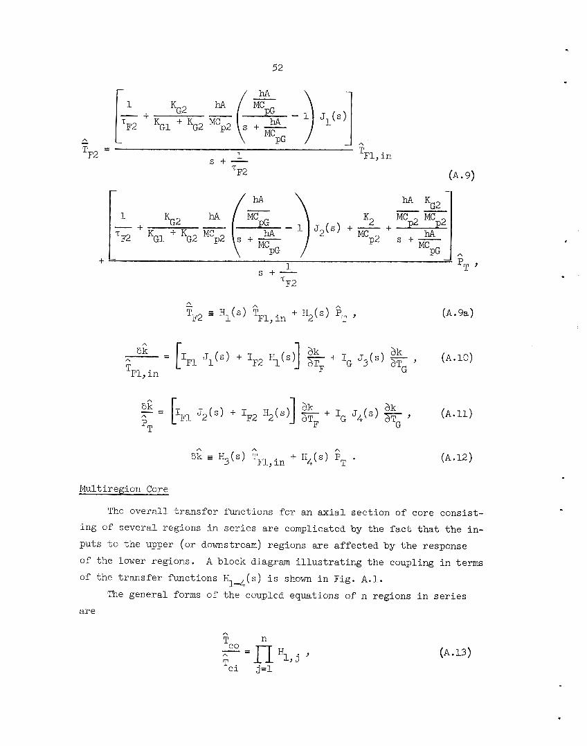
Multiregion Core
The ove ra l l t r a n s f e r flmctions for an axial sec t ion of core cons is t -
i ng of severa l regions i n s e r i e s a r e complicated by t he f a c t t h a t t h e in - pu ts t o t h e upper (or downstream) regions a re a f f ec t ed by t h e response
of t he lower regions. A block diagram i l l u s t r a t i n g t h e coupling i n terms
of the t r a n s f e r functions H14(s) i s shown i n Fig. A . l .
The general forms o f t he coupled equations of n regions i n s e r i e s
a r e
(A.13)
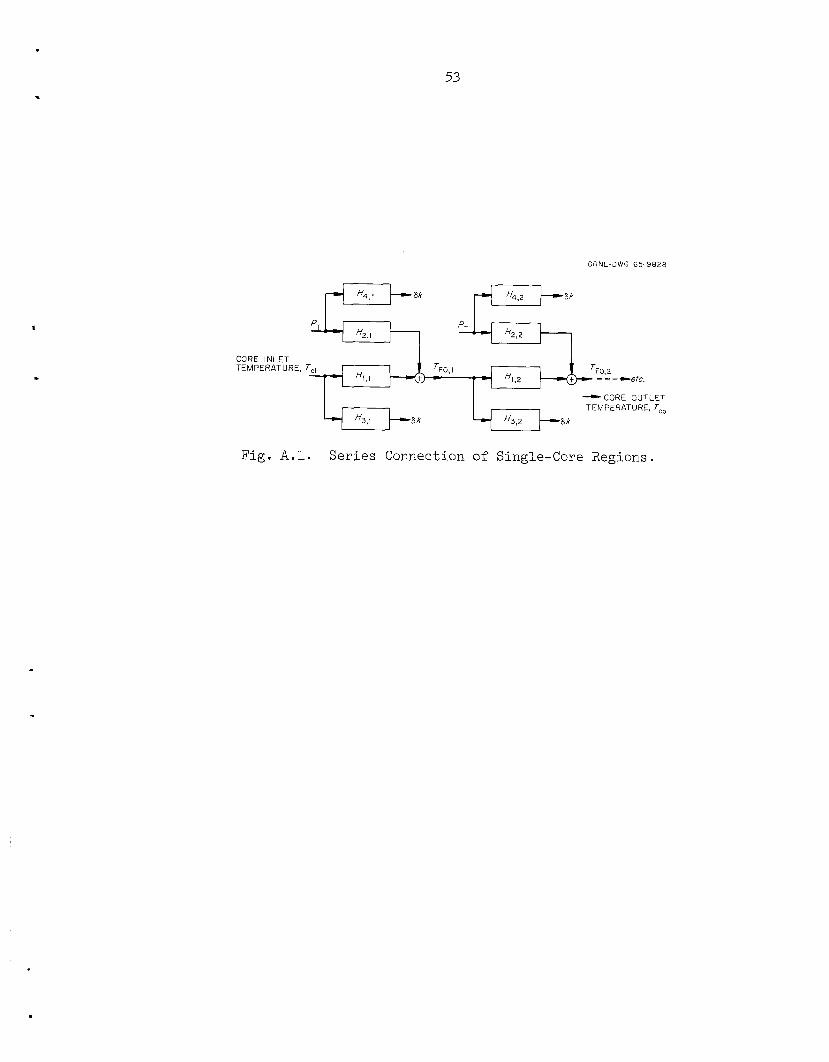
53 .
O R N L - D W G 65-9828
C
CORE INLET TEMPERATURE, T,,
4.1 r - i H1,2 --)CORE OUTLET TEMPERATURE, Tco
Fig. A.l. Series Connection of Single-Core Regions.
54
+ (H2,1 H1,2 H1,3 + H2,2 H1,3 H2,3) H3,4 + ... . (A.16)
- The mean value of the core outlet temperature, %o for m axial sections
in parallel is
m (A.17)
where FF
The total 6k is simply the sum of all the individual contributions.
was added to the MSRE frequency-response code as an afterthought; conse- quently there is some repetition in the calculations. tions of nuclear average temperature contributions from each core region
is the fraction of the total flow in the jth axial section. j
The calculation of nuclear average temperature transfer functions
The transfer fmc-
are
A
= I J ( s ) z H 6 ( s ) , Tc" T~l, in
G 3 n
. . T*
(A. 19)
(A.20)
55
8
A
(A. 21) Tc" pT
y = IG J4(s) z H8(s) ,
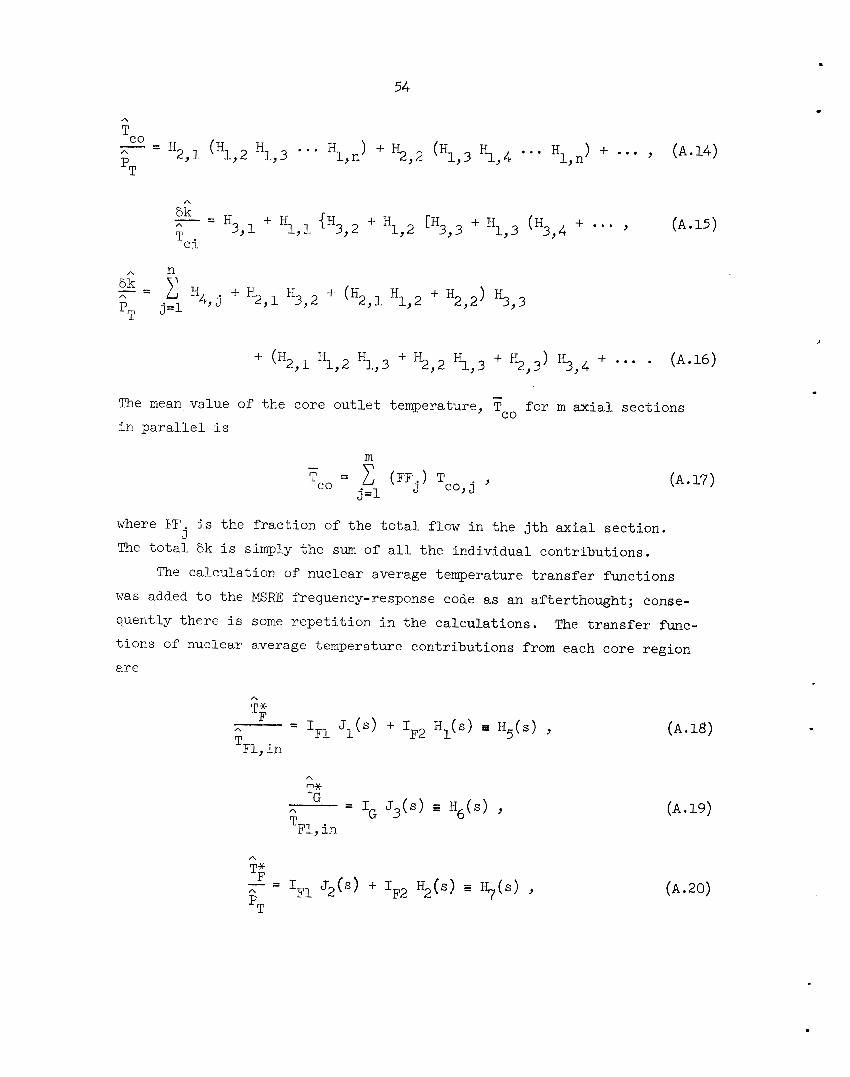
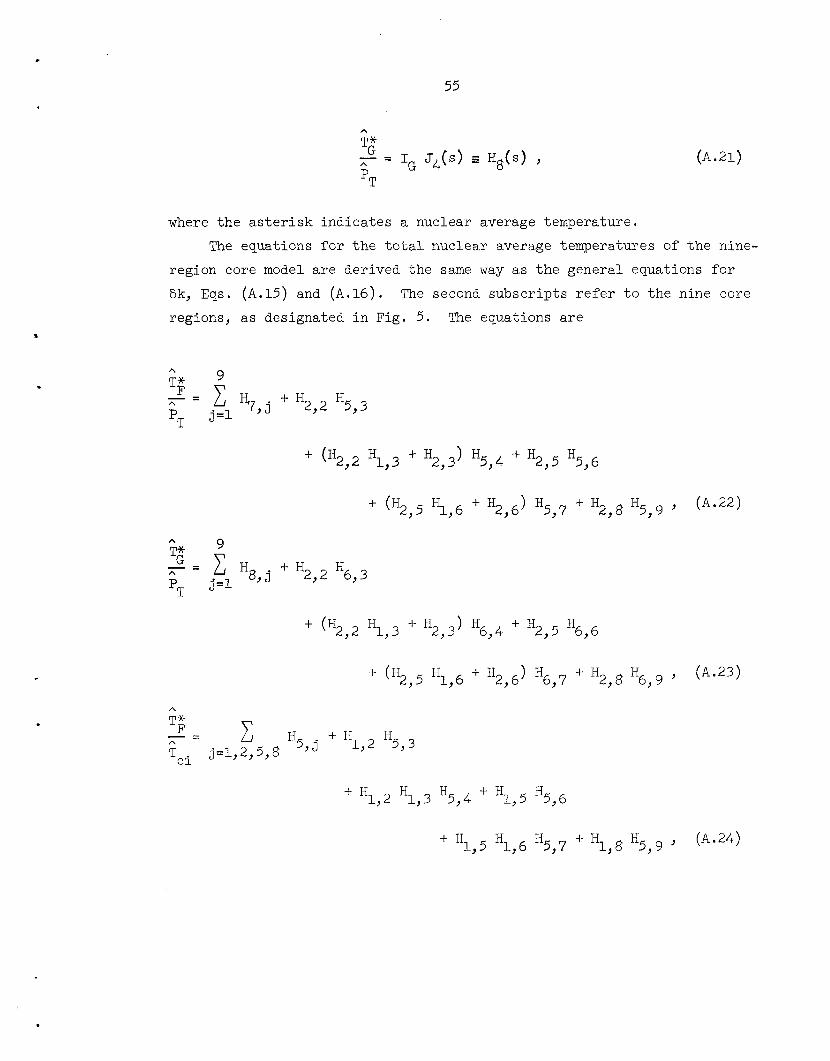
where the asterisk indicates a nuclear average temperature. The equations for the total nuclear average temperatures of the nine-
region core model are derived the same way as the general equations for 6k, Eqs. (A.15) and (A.16). The second subscripts refer to the nine core regions, as designated in Fig. 5. The equations are
9 A
h P, J=1 H B , j H2,2 H6,3
+ ('2,5 H1,6 + H2,6) '6,7 -I- H2,8 H6,9 ' (A.23)
A
H1,5 H1,6 H5,7 + H1,8 H5,9 ' (A.24)
56
A
TG H6,j $- H1,2 H6,3
- = A
Tci j=l, 2,5,8
+ H H H + H H . (A.25) i,5 i,6 6,7 i,8 6,9
Neutron Kinetics
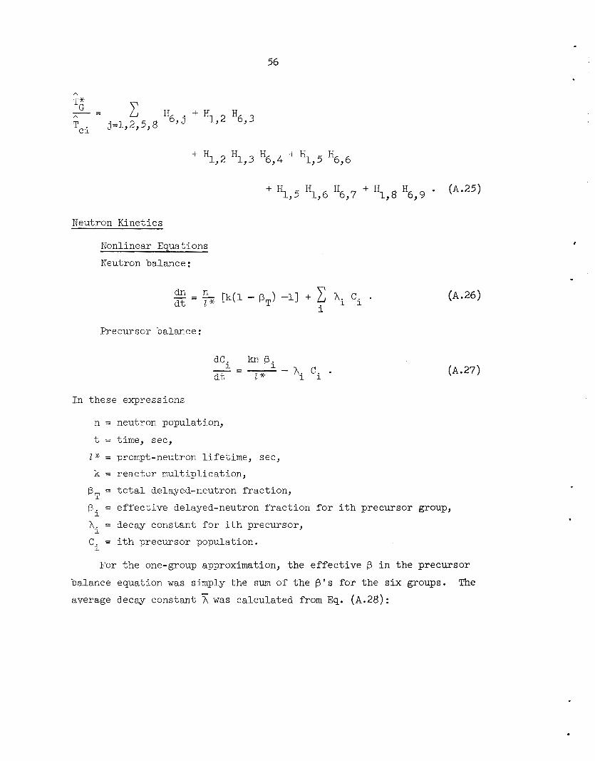
Nonlinear Equations
Neutron balance:
dn n dt l* i - = - [ k ( l - p,) -13 + Ai ci
Precursor balance:
dCi kn Pi dt I * - = - - Ai ci
In these expressions
(A.26)
(A.27)
n =
t = 2 " =
k =
B, =
Bi - Ai -
'i
- - - -
neutron population,
time, see,
prompt-neutron lifetime, sec, reactor multiplication, total delayed-neutron fraction,
effective delayed-neutron fraction for ith precursor group,
decay constant for ith precursor, ith precursor population.
For the one-group approximation, the effective f3 in the precursor
balance equation was simply the sum of the f3's for the six groups.
average decay constant
The was calculated from Eq. (A.28):
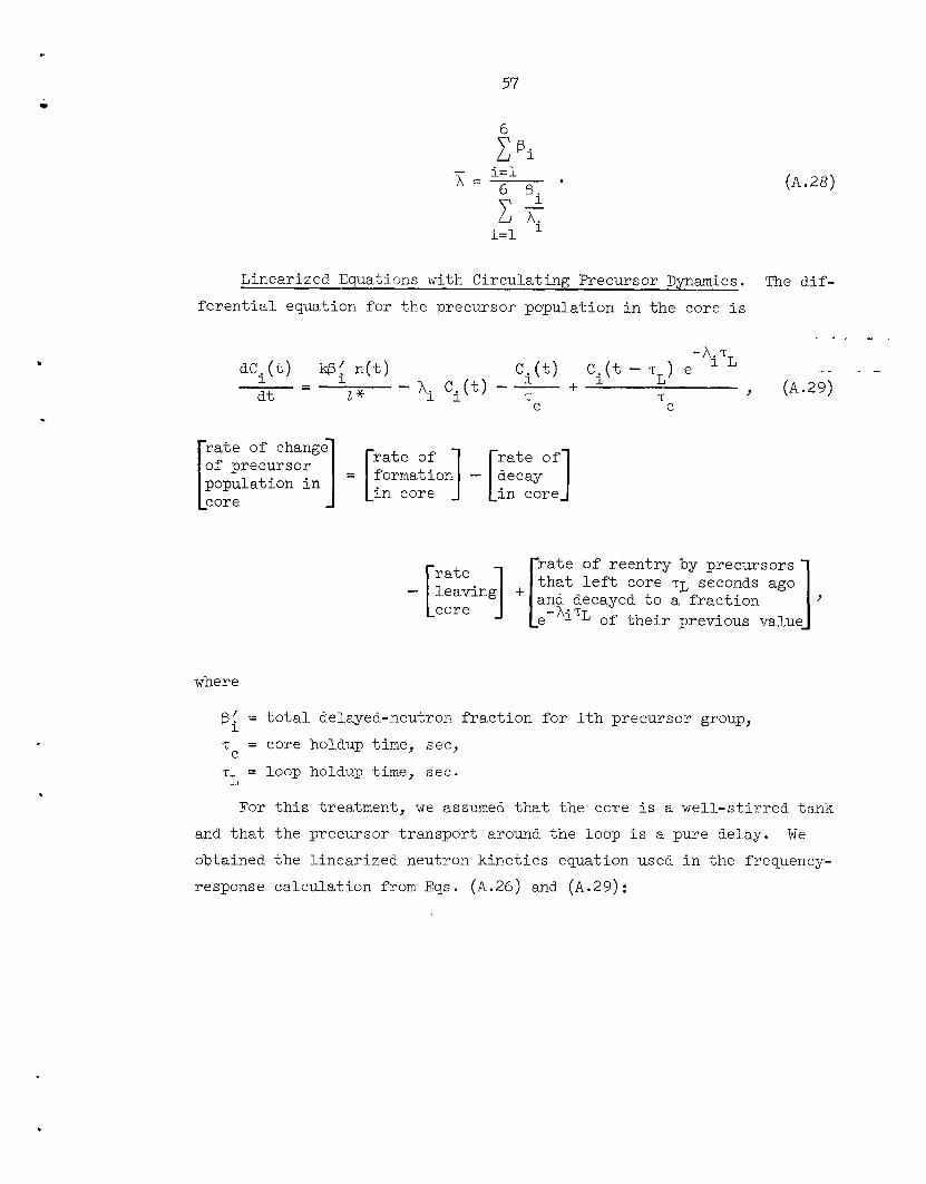
57
(A. 2%)
Linearized Equatims with Circulating Precursor Dynamics.
ferential equation fOY the precursor population in the core is The dif- -
rrate of change] of precursor - population in J - I core
where
inate formation] of - becay rate of ] -in core in core
reentry by precursors core ZL seconds ago to a fraction
of their previous
rate
B! = total delayed-neutron fraction for ith precursor group, T = core holdup time, sec,
T = loop holdup time, sec.
1
C
L For this treatment, we assumed that the core is a well-stirred tank
and that the precursor transport around the loop is a pure delay. We obtained the linearized neutron kinetics equation used in the frequency-
response calculation from Eqs. (A.26) and (A.29) :
.
58
1 - TL ( S +Ai 1
Ai@ f
1 - TL ( s +Ai l - P B T + i
i=l s + A i + - 1 T [I-e
1 ; c - - = ,
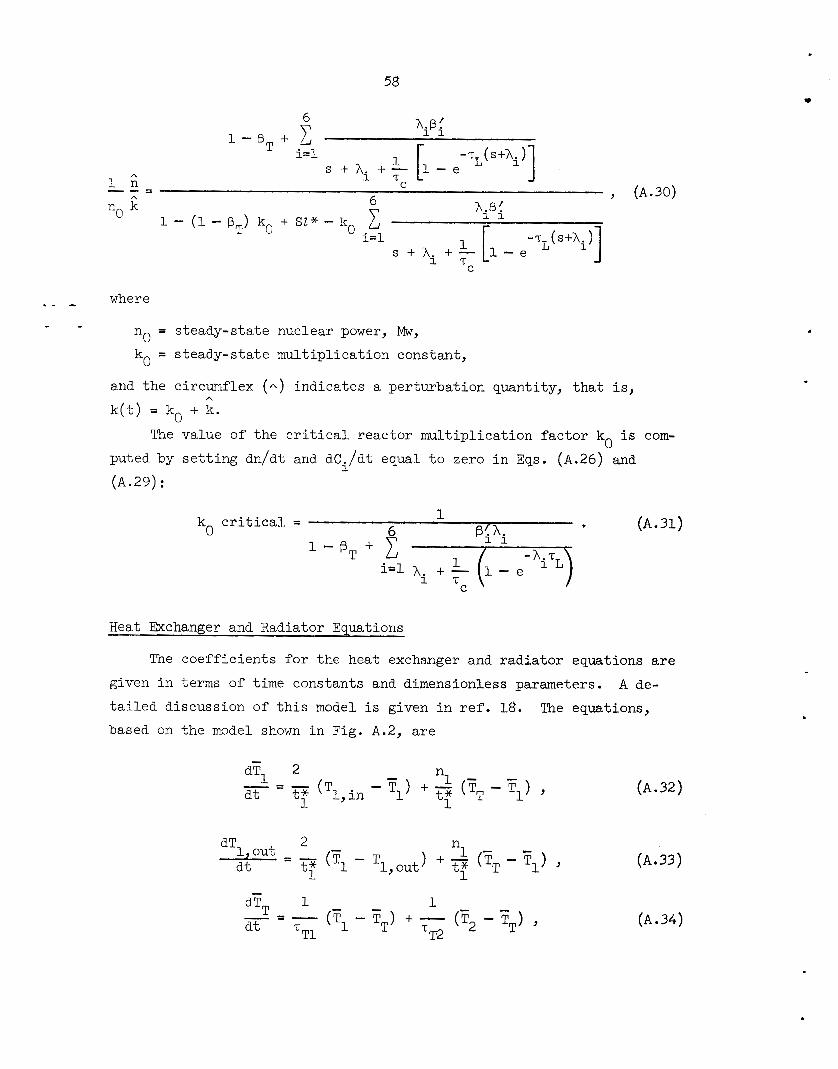
A 0 x R / ? (A.30)
where . - - - - steady-state nuclear power, Mw, no -
ko = steady-state multiplication constant,
and the circumflex ( A ) indicates a perturbation quantity, that is, k(t) = ko + k.
puted by setting dn/dt and dCi/dt equal to zero in Eqs. ( A . 2 6 ) and
(A.29):
A
The value of the critical reactor multiplication factor k 0 is com-
Heat Exchanger and Radiator Equations
The coefficients for the heat exchanger and radiator equations are
given in terms of time constants and dimensionless parameters. tailed discussion of this model is given in ref. 18. based on the model shown in Fig. A.2, are
A de- The equations,
(A.32)
( A . 3 3 )
( A . 3 4 )

59
ORNL-DWG 65-9829
SHELL s
\TUBE T
Fig. A.2. Heat Exchanger and Radiator Tube Model.
- - - - -
.
.
60
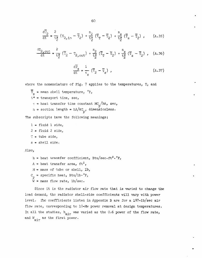
- n s - - 2
- 2 n dT2 - T ~ ) + - (TT - T2) + - (Ts - T2) , tz" - e -
dt t; (T2,in t;
where the nomenclature of Fig. 7 applies to the temperatures, T, -
= mean shell temperature, O F , TS t* = transport time, see,
T = heat transfer time constant MC P /hA, see, n = section length = hA/WC dimensionless.
P' The subscripts have the following meanings:
1 = fluid 1 side,
2 = fluid 2 side,
T = tube side,
s = shell side.
Also,
h = heat transfer coefficient, Btu/sec ft2 OF,
A = heat transfer area, ft2,
M = mass of tube o r shell, lb, C = specific heat, Btu/lb*"F, P W = mass flow rate, lb/sec.
(A. 35)
( A . 3 6 )
(A.37)
and
Since it is the radiator air flow rate that is varied to change the
load demand, the radiator shell-side coefficients will vary with power
level. The coefficients listed in Appendix B are for a lW-lb/sec air flow rate, corresponding to 10-Mw power removal at design temperatures. In all the studies, hair was varied as the 0.6 power of the flow rate,
and Wair as the first power.

61
.
The solutions of the Laplace-transformed transfer function equations
are
A
(2 - n ) + nlB 1 F , I - out
A
T1, in t p + 2
D + (2 - n2 - ns) + T ns s + l ]E S
A
T2, out - - A Y
T2, in t p + 2
DE nl + C (2 - A T1, out z 1 T2, in
2
t p + 2
,
n + (2 -n2 - n s ) A + S
+
S
A
T2, out - - A
T1, in
where
2 n A = n
S t * s + n + 2 + n - s T s + l
S 2 2
1 B = T T T1 T1 A z s + 1 + - - - T2 'T2 T1 T
1 n
t * s + n + 2 ' C = 1 1
D = T2 'T2 T1 T1
T
T TT2 s + l + - - -
T
A
t p + 2
(A .38)
(A .39)
(A.40)
(A. 41)
t*s + n 2 + 2 + n -n2D- S 2 S z s + l
S

62
A
Tl, out h
.
9 - - GIG; 1 - G ~ G ; :
2 F = t * s + n 1 1 + 2 - n l B m
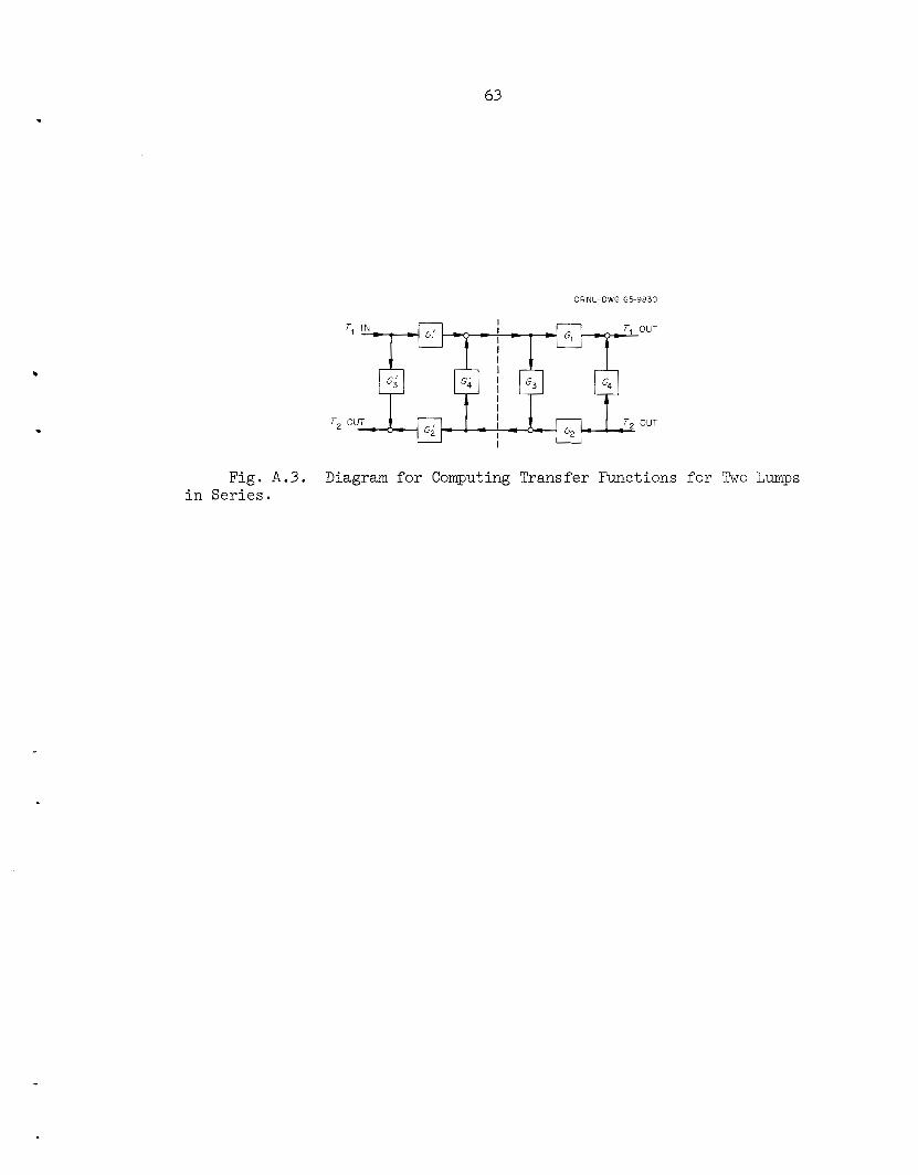
To compute the t r ans fe r functions of an a r b i t r a r y number of equal lumps
connected i n se r i e s , we considered f i rs t the t r ans fe r functions f o r two
lumps i n se r i e s , as i n Fig. A.3, where f o r each lump,
A
T2, out A
- T2, out
G3 - T1,in ?
G;G;G~ = G; +
1 - G3Gi '
The t r ans fe r functions for t h e two combined lumps a r e
- - G1G2Gi G4 + 1 - G ~ G ~
T2,in I comb.
A
T1, out A
(A.42)
(A .43)
(A.45)
To solve fo r more lumps i n se r i e s , we s e t t he primed f'unctions equal t o
the respect ive combined t r ans fe r functions and repeated the computation.
63
ORNL-DWG 65-9830
Fig. A . 3 . Diagram f o r Computing Transfer Functions for Two Lumps i n Ser ies .
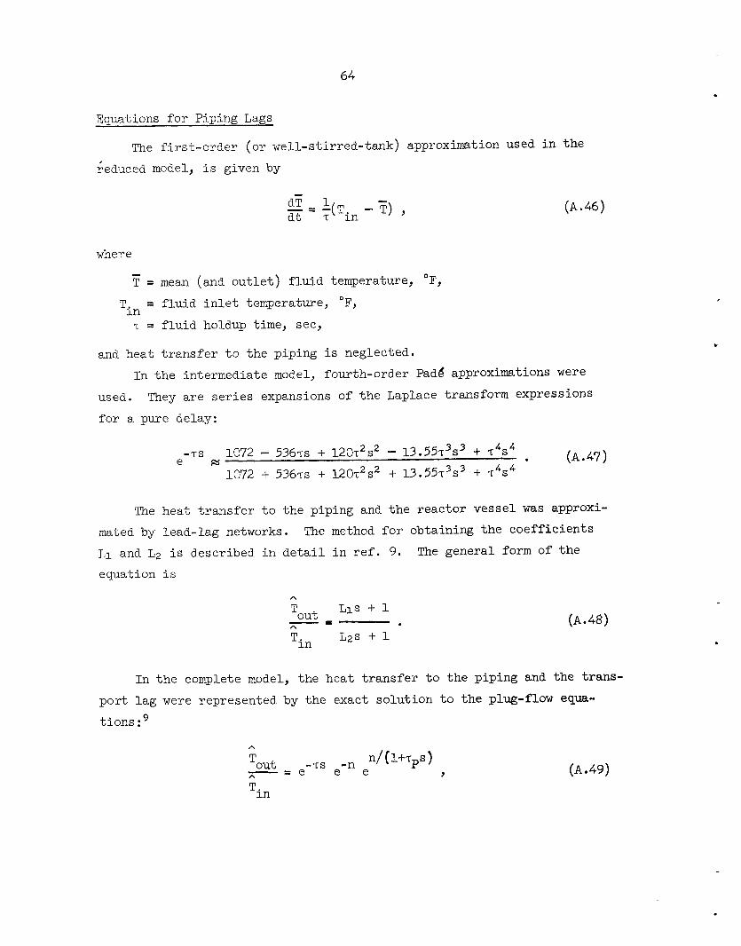
. Equations f o r Piping Lags
The first-order (or well-stirred-tank) approximation used in the
+educed model, is given by
- dT 1 - = -$Tin T) 9 dt
where - T = mean (and outlet) fluid temperature, O F ,
= fluid inlet temperature, O F , Tin T = fluid holdup time, sec,
and heat transfer to the piping is neglected. In the intermediate model, fourth-order Pad6 approximations were
used.
for a pure delay: They are series expansions of the Laplace transform expressions
(A.47) -TS 1072 - 5367s + 120,c2s2 - 1 3 . 5 5 ~ ~ ~ ~ + T ~ S ~
1072 + 5367s + 1 2 0 ~ ~ s ~ + 13.55~'~~ + 7's4 e M
The heat transfer to the piping and the reactor vessel was approxi- mated by lead-lag networks.
Li and L2 is described in detail in ref. 9. equation is
The method for obtaining the coefficients The general form of the
A
LlS + 1 Tout -3c A
L2s + 1 *in
( A . 4 8 )
In the complete model, the heat transfer to the piping and the trans- port lag were represented by the exact solution to the plug-flow equa- tions :
A
Tout - T s -n ./[1+,4 - - e e - e A Y ( A . 4 9 )
t
Tin

65
where
n = section length = hA/WC T = transport lag, see,
P
dimensionless, P’
T = time constant for heat transfer to pipe = MC /hA, see. P
Equations for Xenon Behavior
Xenon was considered only in the present frequency-response model.
Th.e following differential equations were used:
- - - K1X’ - (Kz + K3Po) XG , dt (A.50) dxc
- - a/ - KqI + K5X - KGX’ + K7P , dt G
- = d1 -K~I + K,P , dt
(A. 51)
(A. 5 2 )
where
XG = xenon concentration in graphite, atoms/cc,
X’ = xenon concentration in fuel salt, atoms/cc,
I = iodine concentration in fuel salt, atoms/cc,
P = nuclear power, Mw,
6k = change in reactor multiplication factor due to change in xenon concentrations,
Kl-11 = constants.
Delayed Power Equations
The equation for total thermal power, PT, includes a first-order lag approximation of the delayed nuclear power due to gamma heating:
dn (n - PT) - - - dt dt T 2 (A. 54) - (1 - Kd) - - dPT
g

66
where
= the fraction of flux power delayed, Kd n = flux power, Mw,
= total thermal power, Mw, pT T = effective time constant for the delayed power, see.
g
The frequency response of the thermal power in terms of n is
h
PT (1 - Kd) T s $- 1 - = h
n (A.55)
,
.
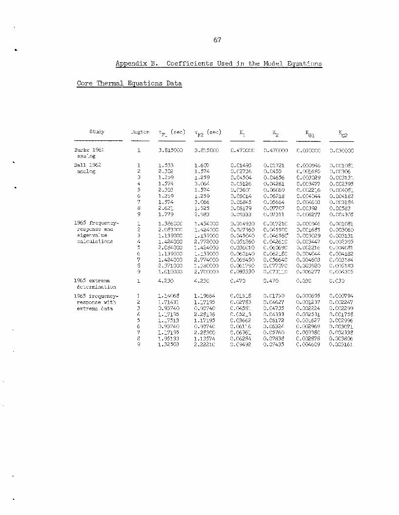
67
Appendix B. Coefficients Used in the Model Equations
Core Thermal Equations Data
Study K1 K2 KGl KG2 ' F 1
3.815000
'F2
3.815000
Region
Burke 1961 analog Ball 1962 analog
0.470000 0.470000 0.030000 0.030000 1
.
. 1.533 2.302 1.259 1.574 2.303 1.259 1.574 2.621 1.779
1.386000 2.083000 1.13 9000 1.424000 2.084000 1.139000 1.424000 2.371000 1.610000
4.230
0.01493 0.02736 0.04504 0.05126 0.03601 0.06014 0.06845 0.06179 0.09333
0.014930 0.027360 0.045040 0.051260 0.036010 0.060140 0.068450 0.061790 0.093330
0.470
1 2 3 4 5 6 7 8 9
1 2 3 4 5 6 7 8 9
1
1.607 1.574 1.259 3.064 1.574 1.259 3.066 1.525 2.983
1.454000 1.424000 1.13 9000
0.01721 0.0455 0.04656 0.04261 0.06069 0.06218 0.05664 0.07707 0.07311
0.017210 0.045500 0.046560' 0.042610 0.060690 0.062180 0.056640 0.077070 0.073110
0.470
0.000946 0.001685 0 . GO302 9 0 . GO3477 0.002216 0.004044 0.004603 0.00392 0.006277
0.000946 0.001685 0 . GO3029 0.003447 0.002216 0.004044 0.004603 0.003920 0.006277
0.030
0.001G81 0.00306 0.003131 0.002395 0.004081 0.004182 0.003184 0.00583 0 . GO4305
0.001081 0.003060 0.003131 0.002395 0.004081 0.004182 0.003184 0.005183 0.004305
0.030
1965 frequency- response and eigenvalue calculations 2.772000
1.424000 1 .' 13 9000 2.774000 1.380000 2.700000
4.230 1965 extrema determination
1965 frequency- response with extrema data
1.14068 1.71431 0.93740 1.17 195 1.17513 0.93740 1.171 95 1.95133 1.32503
1.1%64 1.17 195 0.93740 2.28136 1.17195 0.93740 2.28300 1.13574 2.22210
0.01518 0.02783 0.04581 0.05213 0.03662 0.06116 0.06961 0.06284 0.09492
0.01750 0.04627 0.04735 0.04333 0.06172 0.06324 0.05760 0.07838 0.07435
0.000695 0.001237 0.002224 0.002531 0 . GO1627 0.002 969 0.003380 0.002878 0.004609
0.000794 0.002247 0.002299 0.001758 0.002996 0.003071 0.002338 0.003806 0 . GO3161

Study
Burke 1%1 analog Ball 1962 analog
1965 frequency- response and eigenvalue calculations
1%5 extrema determination 1965 frequency- response with extrema data
Region
1
1 2 3 4 5 6 7 8 9 1 2 3 4 5 6 7 8 9 1
MC PI P2
MC MC PG
(Mw-sec/"F) (Mw. sec/"F) (Mw. sec/"F)
0.763000 0.763000 3.750000
0.0188 0.0638 0.0349 0.0436 0.1080 0.0590 0.0738 0.2970 0.2014 0.015100 0.051200 0.028000 0.035000 0.086600 0.047300 0.059200 0.238000 0.161500 0.750
0.01581 0.05360 0.02931 0.03664 0.09066 0.04952 0.06197 0.24915 0.16907
0.0197 0.0436 0.0349 0.0850 0.0738 0.0590 0.1437 0.1726 0.3380 0.015800 0.034900 0.028000 0.0682 00 0.059200 0.047300 0.115200 0.138400 0.271000 0.750
0.01654 0.03654 0.02931 0.07140 0.06197 0.04952 0.12060 0.14489 0.28370
0.070 0.2114 0.1601 0.2056 0.3576 0.2718 0.3478 0.9612 0.9421 0.070000 0.211400 0.16 0600 0.205600 0.357600 0.271800 0.347800 0.961200 0.942100 3.58
0.070 0.2114 0.1606 0.2056 0.3576 0.2718 0.3478 0.9612 0.9421
0.020000
0.265 X 0.814 x 0.609 x 0.794 x 1.338 x lom3 1.031 X 1.343 x
3.624 x 0.0003 92 0.001204 0.000900 0.001174 0.00197'7 0.001525 0.001985 0.005445 0.005360 0.020
3.685 x
0.588 x 1.806 x 1.35 x 10''
2.965 x 2.287 x 2.977 x
1.761 X
8.167 X loe3 8.04 x
IF1 IF2 IG
1.000000 0. 1.000000
0.02168 0.02197 0.07897 0.08249 0.02254 0.08255 0.08623 0.02745 0.06936 0.021680 0.021970 0.078970 0.082490 0.022540 0.082550 0.086230 0.027450 0.069360 1.0
0.02168 0.02197 0.07897 0.08249 0.06801 0.08255 0.08623 0.02745 0.06936
0.02678 0.06519 0.08438 0.04124 0.06801 0.08%23 0.04290 0.05521 0.03473 0.026780 0.065190 0.084380 0.041240 0.068010 0.088230 0.042 900 0.055210 0.034730 0.0
0.02678 0.06519 0.08438 0.04124 0.06801 0.08823 0.04290 0.05521 0.03473
0.04443 0.08835 0.16671 0.12077
0.09181 0.1742 9 0.12612 0.08408 0.10343 0.04443 0 0.088350 o\
0.166710 03
0.12 077 0 0.091810 0.174290 0.12612 0 0.084080 0.103430 1.0
0.04443 0.08835 0.16671 0.12077 0.09181 0.1742 9 0.12612 0.08408 0.10343
c
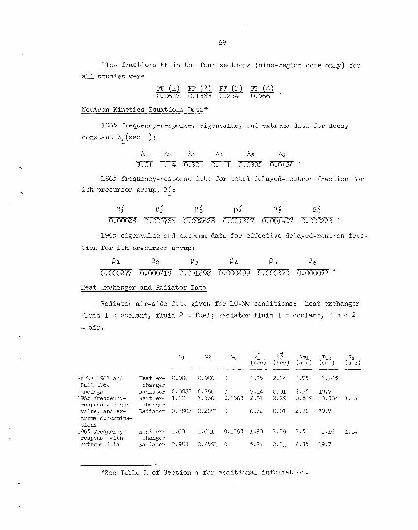
.
.
Flow fractions FF in all studies were
FF (1) 0.0617
the four
FF (2) 0.1383
69
sections (nine-region core only) for
FF (3) FF (4) 0.234 0.566 ‘
Neutron Kinetics Equations Data*
1965 frequency-response, eigenvalue, and extrema data for decay constant A ~ ( see-’) :
A1 A2 A3 A4 A5 A6 I_---
3.01 1.14 0.301 0.111 0.0305 0.0124 ’
1%5 frequency-response data for total delayed-neutron fraction for ith precursor group, f3‘- i’
si Bz/ fG Pi @; !G 0.000766 0.002628 0.001307 0.001457 0.000223
1965 eigenvalue and extrema data for effective delayed-neutron frac-
tion for ith precursor group:
B 1 B2 B 3 B 4 B5 p6
0.000277 0.000718 o.001698 0.000499 0.000373 0.000052
Heat Exchanger and Radiator Data
Radiator air-side data given for 10-Mw conditions: heat exchanger
fluid 1 = coolant, fluid 2 = fuel; radiator fluid 1 = coolant, fluid 2
= air.
n l n2 ns ts” t$ TT1 TT2 TS ( sec) ( see) (see) (see) (see)
Burke l%l and Heat ex- 0.980 0.906 0 1.75 2.24 1.75 1.165 B a l l 1962 changer analogs Radiator 0.0882 0.260 0 7.14 0.01 2.35 19.7
response, eigen- changer value, and ex- Radiator 0.8803 0.2591 0 6.52 0.01 2.35 19.7 trema determina- t i o n s
response with changer extrema data Radiator 0.983 0.2591 0 5.84 0.01 2.35 19.7
1%5 frequency- Heat ex- 1.10 1.366 0.1363 2.01 2.29 0.569 0.304 1.14
1965 frequency- Heat ex- 1.60 1.611 0.1363 1.80 2.29 2.5 1.16 1.14
*See Table 1 of Section 4 for additional information.

70
Piping Lag Data
1%5 Frequency Response with
Burke Ball 1965 Frequency 1965 Extrema Response and 1%1 1962 Determinations Eigenvalue Extrema Data
Core to heat n exchanger T 3.09 5.72 5.77 5.77 6.30
P T
Heat ex- n 0.155 0.155 0.155 changer to T 9.04 9.02
15.15 P core z 8.67 15.15
Heat ex- n 0.27 0.27 changer to T 5.2 5.2 4.71 radiator T 6.67 6.67 P Radiator n 0.40 0.40 to heat T 10.11 10.11 8.24 exchanger z 6.67 6.67 P
8.67
4.71
8.24
9.47 15.15
0.27 4.22 6.67
0.40 7.38 6.67
The coefficients of the lead-lag approximation for f l u i d heat trans- fer to the piping apply to the Ball 1962 analog study:
Heat Exchanger Heat Exchanger Radiator to to Core to Radiator Heat Exchanger
L1 14.35 5.84 5.58
L2 16.67 7.69 8.33
Xenon Equation Data
Data for 1965 frequency response and frequency response with extrema data :
Kl = 1.587 X lom6 K~ = 2.885 x K2 = 2.2575 X Kg 2 . 9 X l om5 K 3 = 1.654 X
K4 = 2.84 X
K5 = 1.0714 X
K6 = 1.059 X lom3
K9 = 9.47 X
K l o = 3.07 X
K11 = 1.03 x
.
Delayed Power Equation Data
See Table 1 of Section 4.
71
Amendix C. General DescriDtion of MSRE Frequency-Response Code
J
The MSRE frequency-response code (MSFR) is written in FORTRAN IV language for the IBM 7090 computers at the Oak Ridge Central Data Pro- cessing Facility. This language has builtin capabilities for handling complex algebra that result in considerable savings of programming effort.
MSFR uses transfer function techniques (rather than matrix methods ) It exploits the fact that a reactor sys- to compute frequency response.
tem is made up of separate components, each having a certain number of inputs and outputs, which tie in with adjacent components. tines written for each subsystem were useful in other reactor and process
dynamics calculations. The MAIN program of MSFR performs input, output,
and supervisory chores, and calls the subroutines. A subroutine called CLOSED must be written to compute the desired closed-loop transfer func-
tions from the component transfer functions.
The subrou-
The transfer function approach has several advantages 6ver the ma-
trix methods :
1. Input parameters are the physical coefficients of the subsys- tems, rather than sums and differences.
input data easy, it allows the computer to carry out the sum-difference-
type arithmetic internally. Several matrix type computations for which the matrix coefficients were generated "carefully" with long slide rules resulted in large errors in the frequency response.
This not only makes generating
2 . The frequency response of distributed-parameter models can be
computed exactly with MSFR, while most matrix calculations are limited to lumped-parameter models.
3. MSFR calculations are much faster. The 7090 can put out between 1000 and 2000 frequency-response points per minute for the complete model.
longer.
Typical running times for current matrix calculations are much
The matrix technique has the advantages that special programming
is not required for each different problem, and no algebraic manipulations
of the equations are required. Also, matrix manipulations can be used

72 *
for optimization calculations, eigenvalue calculations, time-response
calculations, and possibly many others, all with the same input data.
The advantages of both methods were exploited in this study. The following subroutines of MSFR have potential as generally use-
ful packages : h A
1. PWR, which calculates the frequency response (N/6k) of the nuclear kinetics equations for up to six groups of precursors, with an
option for including circulating precursor dynamics.
2 . CLMP, which computes the frequency response of a "typical" core
region (as noted in Appendix A). Inputs are power and inlet temperature, and outputs are outlet temperature, nuclear average temperatures, and 6k.
3. COR9, which calculates the overall frequency responses of the
MSRE nine-lump core model using CLMP outputs. 4 . LHEX, which calculates the transfer functions of a lwnped-
parameter heat exchanger (as in Appendix A), with an input option for
solving for up to 99 typical sections in series in a counterflow con- figuration.
5 . PLAG, which computes the frequency response of piping lags for
an arbitrary number of first-order series lags, a fourth-order Pad6 ap-
proximation, or a pure delay, or combinations of these, with heat trans-
fer to the piping.
Figure C . l shows the block diagram used as a guide to compute the closed-loop transfer functions. are N/6k (closed loop), Nyquist stability information, nuclear average temperatures ̂T$& and !?'*/6$, and ?co/& and !?'ci/&.
Typical outputs of the subroutine CLOSED A h
G
Several commonly used transfer fbnctions are
and A
N
t
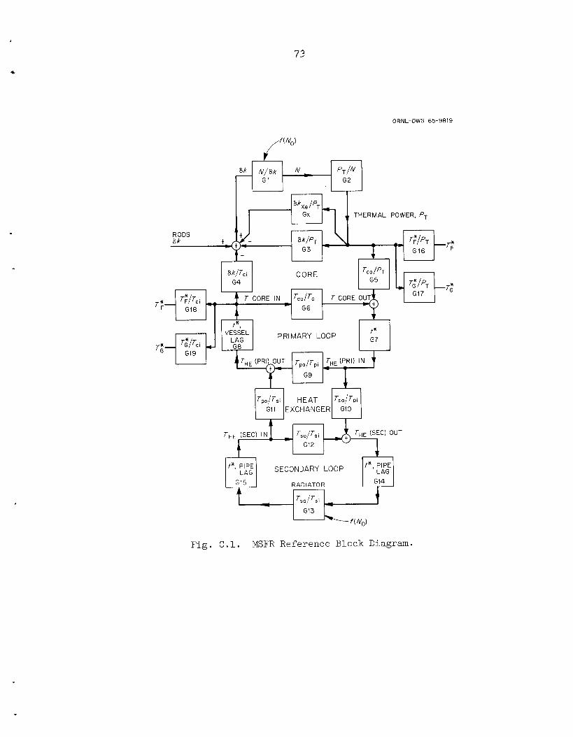
c
73
ORNL-DWG 65-9819
SECONDARY LOOP
Fig. C.l. MSFR Reference Block Diagram.

74
Each of these closed-loop equations can be written as a single
FORTRAN IV statement, so it is a simple matter to generate different functions. An option is also available in MSFR to print out all the internal or component transfer functions. FORTMN IV listings, decks, and input information may be obtained from S. J. Ball.
.
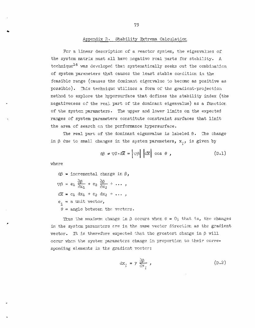
75
Appendix D. Stability Extrema Calculation
J
For a linear description of a reactor system, the eigenvalues of A the system matrix must all have negative real parts for stability.
technique16 was developed that systematically seeks out the combination
of system parameters that causes the least stable condition in the feasible range (causes the dominant eigenvalue to become as positive as possible). method to explore the hypersurface that defines the stability index (the
negativeness of the real part of the dominant eigenvalue) as a function
of the system parameters. The upper and lower limits on the expected ranges of system parameters constitute constraint surfaces that limit the area of search on the performance hypersurface.
This technique utilizes a form of the gradient-projection
The real part of the dominant eigenvalue is labeled p . The change in p due to small changes in the system parameters, xI, is given by
where
@ = incremental change in B,
+ ... , aB OB = el ax, + e2 ax,,
e = a unit vector, i 8 = angle between the vectors.
Thus the maximum change in f3 occurs when 0 = 0; that is, the changes in the system parameters are in the same vector direction as the gradient vector. It is therefore expected that the greatest change in @ will occur when the system parameters change in proportion to their corre- sponding elements in the gradient vector:

76
where y is a real positive coefficient whose magnitude is chosen to
insure that constraints are satisfied.
It is clear that the calculated values of the components ofVB are the key quantities in implementation of this method. The method for findingvp can be developed from the characteristic equation for the system given in determinant form:
where
A = the system matrix,
s E an eigenvalue of A,
I = the unit diagonal matrix.
We now write D with some arbitrary eigenvalue, s k' factored out:
D = (S - sk) F(s ) = 0 , ( D . 4 )
where F ( s ) is a nonzero determinant if s k is a simple eigenvalue.
differentiate Eq. ( D . 4 ) with respect to an element, aij, of the matrix,
A, and with respect to s:
We
We then evaluate Eqs. ( D . 5 ) and(D.6) for s = sk and take their ratio to
get Eq. ( D . 7 ) :

77 c
The derivative, aD/aaij, is just the cofactor of a in [A - SI], and ?ID/& is the negative of the sum of the cofactors of diagonal ele-
ments of [A - SI].
ij
Thus Eq. (D.5) may be written
f=l
If we choose s s is just p. Since a is real, we may write
to be the least negative eigenvalue, the real part of k
k ij
The derivative with respect to a system parameter, xI, is easily ob- tained from Eq. (D.9), since the following relation holds:
We use this in Eq. (D.9) to obtain
(D.10)
The usefulness of Eq. (D.lO) rests on the ability to calculate the system eigenvalue, sk, to give [A - ski]. plished by using one of the standard eigenvalue computation methods, such as Parlett’s method” or the Q,R method.14
This may be readily accom-
The cofactors in Eq. (D.lO) could be calculated directly with a
method such as Gaussian elimination. However, this tedious procedure may be circumvented by application of a useful theorem from matrix algebra.
c
78 3
It is known that the cofactors of parallel lines in a matrix with order
n and rank n - 1 are proportional.20 Since [A - S,I] is a matrix with these properties, the cofactor calculation may be simplified. For in- stance, if the cofactors of the first row and first column of [A - ski] are calculated, all other cofactors are given by
- ‘i j
‘il ‘lj n
k 1 (D.ll)
Use of Eq. (D.ll) to find the cofactors shown in Eq. (D.lO) gives a prac- tical method for finding the derivatives $3/ax, needed to carry out the gradient-projection step shown in Eq. ( D . 2 ) .
Gradient methods are useful for finding local extrema for nonlinear
problems. However, it may be possible for the surface of @ versus sys-
tem parameters to have many peaks. for handling this provlem is to use multiple starts. The computer code developed to implement this method is set up to use multiple starts au-
tomatically.
The only technique currently suitable
The procedure for carrying out the maximization from a given base
point is to recalculate the eigenvalues for several new parameter sets
specified by steps out the gradient vector. system with the largest value of p is then used as a new starting point. This is repeated until a maximum within the constrained set of system parameters is found.
me point that gives the
79
ORNL- TM- 1070
Internal Distribution
1. R. K. Adams 2. G. M. Adamson 3. R. G. Affel 4. L. G. Alexander 5. A. H. Anderson 6. R. F. Apple 7. C. F. Baes 8. J. M. Baker 9. M. A. Baker
35. S. E. Beall 36. E. S. Bettis 37. F. F. Blankenship 38. R. Blumberg 39. E. G. Bohlmann 40. C. J. Borkowski 41. G. H. Burger 42. 0. W. Burke 43. S. Cantor 44. W. L . Carter 45. G. I. Cathers 46. E. L. Compere 47. J. A. Conlin 48. W. H. Cook 49. L. T. Corbin 50. G. A. Cristy 51. J. L. Crowley 52. F. L. Culler 53. D. G. Davis 54. S. J. Ditto 55. R. G. Donnelly 56. F. A. Doss 57. N. E. Dunwoody 58. J. R. Engel 59. E. P. Epler 60. W. K. Ergen 61. D. E. Ferguson 62. A. P. Fraas 63. E. N. Fray 64. H. A. Friedman 65. D. N. Fry 66. J. H Frye, Jr. 67. C. H. Gabbard 68. R. B. Gallaher 69. W. R. Grimes 70. A. G. Grindell 71. R. H. Guymon
1C+34. S. J. Ball
72. 73. 74. 75. 76. 77. 78. 79. 80. 81. 82. 83.
84-108. 109. 110. 111. 112. 113. 114. 115. 116. 117. 118. 119. 120. 121. 122. 123. 124. 125. 126. 127. 128. 129. 130. 131. 132. 133. 134. 135. 136. 137. 138. 139. 140. 141. 142.
P. H. Harley C. S. Harrill P. N. Haubenreich G. M. Herbert P. G. Herndon V. D. Holt
A. Houtzeel T. L. Hudson I?. R. Kasten R. J. Ked1 M. J. Kelly T. W. Kerlin S. S. Kirslis D. J. Knowles A. I. Krakoviak J. W. Krewson B. R. Lawrence C. G. Lawson R. B. Lindauer M. I. Lundin R. N. Lyon J. H. Marable C. D. Martin C. E. Mathews H. G. MacPherson H. C. McCurdy W. B. McDonald H. F. McDuffie C. K. McGlothlan L. E. McNeese A. J. Miller W. R. Mixon R. L. Moore H. G. O'Brien P. Patriarca H. R. Payne A. M. Perry H. B. Piper B. E. Prince J. L. Redford M. Richardson R. C. Robertson J. C. Robinson H. C. Roller
H. C. Savage
P. P a Holz
D. P. ROUX
143. H. W. Savage 144. A. W. Savolainen 145. D. Scott 146. H. E. Seagren 147. J. H. Shaffer 148. M. J. Skinner 149. A. N. Smith 150. P. G. Smith 151. W. F. Spencer 152. I. Spiewak 153. R. C. Steffy 154. H. H. Stone 155. R. S. Stone 156. A. Taboada 157. J. R. Tallackson 158. R. E. Thoma 159. G. M. Tolson 160. D. B. Trauger 161. W. C. Ulrich
162. 163. 164. 165. 166. 167. 168. 169. 170. 171. 172. 173.
174-175. 176-177. 1'78-179. 180-184.
185.
B. H. Webster A. M. Weinberg K. W. West M. E. Whatley J. C. White G. D. Whitman R. E. Whitt H. D. Wills J. V. Wilson L. V. Wilson M. M. Yarosh MSRP Director ' s Office,
Reactor Division Library Central Research Library Document Reference Section Laboratory Records Department Laboratory Records, RC
Rm. 219, 9204-1
External Distribution
186-18'7. D. F. Cope, AEC, OR0 188. R. W. Garrison, AEC, Washington, D.C. 189. S. H. Hanauer, University of Tennessee, Knoxville 190. D. C. Keeton, Tennessee Valley Authority, EGCR Site 191. H. M. Roth, AEC, OR0 192. R. F. Saxe, North Carolina State University, Raleigh, N.C. 193. W. L. Smalley, AEC, OR0 194. S. E. Stephenson, University of Arkansas, Fayetteville, Ark. 195. M. J. Whitman, AEC, Washington, D.C.
196-210. Division of Technical Information Extension