sspta for windows users guide
TRANSCRIPT

September 2010
SSSSimplified
SSSSpace
PPPPayload
TTTThermal
AAAAnalyzer
Developed by:
Nicosoft Technologies
P.O. Box 192
Grasonville, MD 21638
SSPTA Contact: Nick Teti Email: [email protected] Web: www.sspta.com
i
IIIINTRODUCTIONNTRODUCTIONNTRODUCTIONNTRODUCTION Chapter 1Chapter 1Chapter 1Chapter 1 First, I would like to thank you for choosing SSPTA. The Simplified Space Payload
Thermal Analyzer developed by Arthur D. Little for the NASA/GSFC has been
running on a VAX 11/780 and MICROVAX II for years in the thermal analysis and
design of spacecraft which include: COBE, UARS, SSBUV, BBXRT, SPARTAN,
PEGSAT, SMEX and others. The Microsoft Windows version of SSPTA has many
advantages over the original VAX version. Improvements have been made to simplify
the user interface, and enhance the speed and efficiency of programs by improving
the computational methods used in SSPTA.
SSPTA Overview
The basic features of SSPTA are:
Geometric model generation (2000 surfaces)
Black body radiative view factors
Shadow factors
ASCRIPTF radiation couplings
Incident flux intensities
Environmental absorbed powers
Interfaces to SINDA, FEMAP and TAK
SSPTA has proven to be an effective thermal analysis tool in both the government
and industry for years. And now with the technological advances in personal
computers, SSPTA allows thermal engineers to perform mainframe type analysis on
their PC's.

ii
Introduction
Preface
Experience with free-flying and shuttle-mounted space payloads in the current
era of reduced budgets has led to a continuing need for an easier-to-use and
more cost-effective capability for payload thermal analyses. To meet these
needs, NASA Goddard Space Flight Center funded Arthur D. Little, Inc., to
develop the Simplified Space Payload Thermal Analyzer (SSPTA): a software
package that simplifies the procedures for conducting a sophisticated thermal
analysis of orbiting payloads. SSPTA, through the use of an integrated set of
thermal subprograms and stored data files, permits a complete, end-to-end,
thermal analysis with a minimum of engineering related effort on the part of
the user. The Simplified Space Payload Thermal Analyzer (SSPTA)
developed for NASA/GSFC is now available for personal computers.
NASA/GSFC has been running SSPTA on a VAX 11/780 and MICROVAX
II for years in the thermal analysis and design of spacecraft which include:
COBE, UARS, SSBUV, BBXRT, SPARTAN, PEGSAT, SMEX and others.
The purchasers of SSPTA understand that SSPTA is a program developed by
A.D. Little under contract for the NASA/GSFC. The owners of SSPTA
understand that they have purchased a version of NASA GSFC's VAX version
(3.0) that has been modified to run on a personal computer. The modifications
made are protected by the United States copyright law.
The purpose of this manual is to provide the SSPTA user with the necessary
information to run and use all the features of the program. It describes the
functional elements of SSPTA, the inputs to and outputs from the elements of
the program, including program options. For several SSPTA programs, the
manual describes the theory and numerical methods being utilized.

iii
Introduction
Background
The Simplified Space Payload Thermal Analyzer (SSPTA) was originally
conceived to analyze payloads mounted in the cargo bay of the orbiter.
Through years of use it has also become a useful analytical tool for general
thermal analyses. The program's primary objective is to provide an
easier-to-use and more cost-effective capability than is otherwise available for
the thermal analysis of payloads. SSPTA is a relatively new program,
however, the concepts used in the program are derived from proven
technology and represent an integration of several programs previously used
independently for many years in the thermal analysis of spacecraft. SSPTA
can meet the needs of experience thermal engineers, who may or may not
possess computer experience, as well as the needs of junior engineers and
computer specialists, with little thermal analysis experience. The input is
simple and frees the user, as much as possible, from the concerns of disk
space, data transfer between programs and strict data formats.
The SSPTA program is internally dimensioned to handle up to 2000 radiation
surfaces and up to 600 thermal nodes. The total running time necessary for a
complete thermal analysis of a space payload will depend largely on the
degree of detail in the geometry model used for radiation computations. Most
of the computer time is typically used to determine radiative view factors and
orbital flux shadow factors with the model. SSPTA's capability to thermally
analyze complex geometric shapes is of particular importance for structures of
multiple payloads like those mounted in the cargo bay of the orbiter.
iv
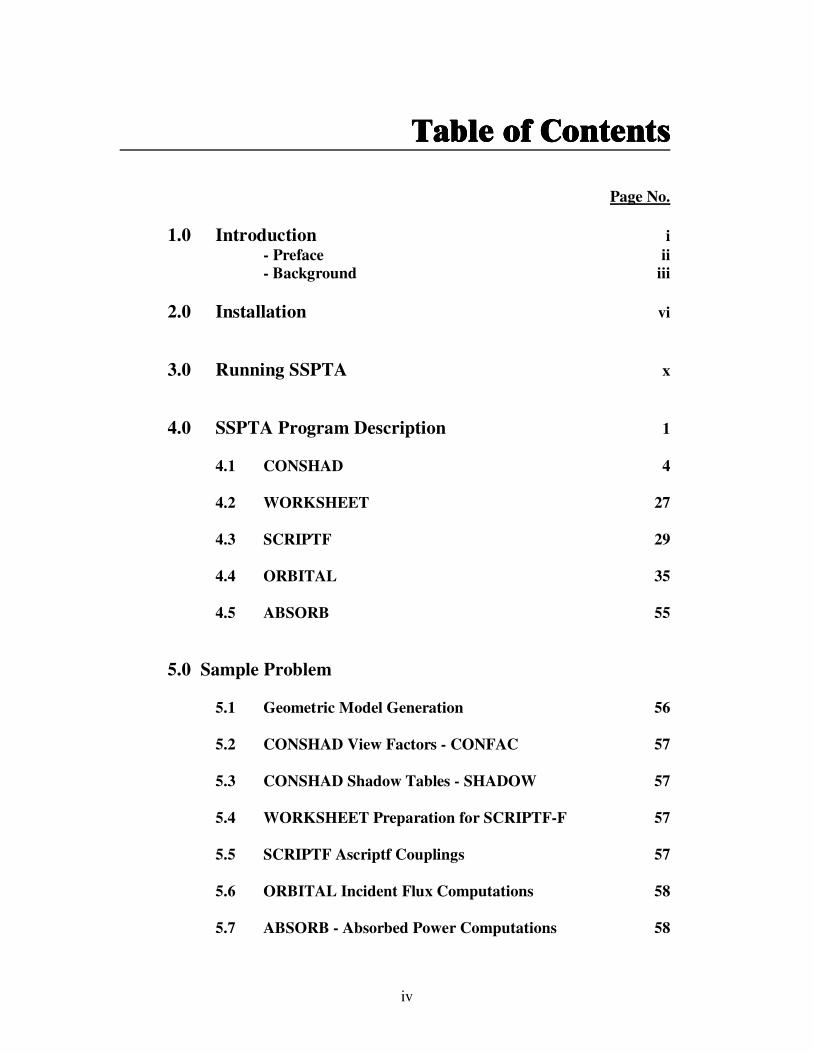
Table of ContentsTable of ContentsTable of ContentsTable of Contents
Page No.
1.0 Introduction i
- Preface ii
- Background iii
2.0 Installation vi
3.0 Running SSPTA x
4.0 SSPTA Program Description 1
4.1 CONSHAD 4
4.2 WORKSHEET 27
4.3 SCRIPTF 29
4.4 ORBITAL 35
4.5 ABSORB 55
5.0 Sample Problem
5.1 Geometric Model Generation 56
5.2 CONSHAD View Factors - CONFAC 57
5.3 CONSHAD Shadow Tables - SHADOW 57
5.4 WORKSHEET Preparation for SCRIPTF-F 57
5.5 SCRIPTF Ascriptf Couplings 57
5.6 ORBITAL Incident Flux Computations 58
5.7 ABSORB - Absorbed Power Computations 58

v
Table of Contents
Page No.
6.0 APPENDICES
Appendix A SSPTA UTILITY PROGRAMS A-1
Appendix B Description of Numerical Methods B-1
used in CONSHAD
Appendix C Description of Numerical Methods C-1
used in ORBITAL
Appendix D Description of Enhanced Geometry D-1

vi
INSTALLATIONINSTALLATIONINSTALLATIONINSTALLATION Chapter 2Chapter 2Chapter 2Chapter 2 System Requirements
The items listed below are considered to be a minimum operating
environment for running SSPTA:
XP Pro or Home or Windows 7
512 MB RAM
.

vii
Installation
LICENSE AGREEMENT
This is a license agreement between you, the end user, and Nicosoft
Technologies. For the purposes of this agreement "software" is defined as any
source code, executables, object code libraries, copy protection device(s), and
product documentation included in the package. Using the software indicates
your acceptance of these terms and conditions. If you do not agree with the
terms and conditions of the license agreement, promptly remove the software
from your computer. This software is protected by United States copyright
law.
LICENSE
The SSPTA software license is a "single user" license. The licensee is
authorized to:
personally use software on any machine.
make archival copies of the software for the sole purpose of
backing-up the software and protecting your investment from loss.
You MAY NOT:
Give a copy of this software or your spare set of disks to another
person; unless authorized to do so.
Use the software on any service bureau, time sharing interactive cable
system, or more than one workstation in any network of single user
computers;
Rent or lease a copy of the software to or from another party.
COPYRIGHT
Information in this document is subject to change without notice and does not
represent a commitment on the part of Nicosoft Technologies. The software
described in this document is furnished under a license agreement. The
software may be used or copied only in accordance with the terms and
conditions of the agreement. This document is protected by federal copyright
law.

viii
Installation
Limited Warranty
The SSPTA software is warranted free from defects in material and
workmanship, assuming normal use, for a period of 90 days. Except for the
express warranty set forth above, there are no other warranties, express or
implied, by statute or otherwise, regarding the disks and related materials.
Nicosoft Technologies shall not be liable for any damages, including but not
limited to any loss of profits, loss of savings, or any other incidental or
consequential damages resulting from the use or inability to use this software.
You, the user, assume all risks and responsibilities as to the results and
performance of this software and manual.
You acknowledge that you have read this agreement, understand it and agree
to be bound by the terms and conditions listed herein. You further agree that
this is the complete and exclusive agreement between you, the user, and
Nicosoft Technologies and that this agreement supersedes all prior
agreements, written or oral.

ix
Running SSPTARunning SSPTARunning SSPTARunning SSPTA Chapter 3Chapter 3Chapter 3Chapter 3
SSPTA for Windows File Manager
1. Select File New from the SSPTA for Windows File Manager to create the
SSPTA input files (.CVW, CSH, .WRK, .SCF and .ORB).
2. CONFAC computes the Black Body View Factors. Enter ‘CONFAC Run
Title’ in the data field provided. Typically the Default values are fine;
however, it is important that you verify that the ‘Engineering Units of
Geometry’ is set appropriately. This selection should match the units used to
generate the Geometric Math Model (GMM) for the SSPTA *.GEO file.

x
Running SSPTA
3. SHADOW computes the Black Body Projected Areas. Enter ‘SHADOW Run
Title’ in the data field provided. Typically the Default values are fine;
however, it is important that you verify that the ‘Engineering Units of
Geometry’ is set appropriately. This selection should match the units used to
generate the Geometric Math Model (GMM) for the SSPTA *.GEO file.
4. WORKSHEET is a utility subroutine whose sole purpose is to aid in the
preparation of optical property and node number assignments for the surfaces
contained in the SSPTA GMM. The file generated by WORKSHEET is used
as input to SCRIPTF, the SSPTA subprogram that computes Gray Body
Radiation Exchange Factors (RADKs).

xi
Running SSPTA
Enter the number of surfaces contained in the GMM, in the data entry field, “Number
of table rows’. File Manager will generate the WORKSHEET data entry fields where
the user provides the SINDA node numbers and the solar absorptance and IR
emittance surface property data. The surface property data can be entered as values or
as groups. See Section 4.2
5. SCRIPTF computes the Gray Body Radiation Exchange Factors (RADKs)
that is used for input to the Thermal Analyzer SINDA/FLUINT or TAK. See
Section 4.3 for additional information on SCRIPTF.

xii
Running SSPTA
6. ORBITAL computes the Black Body Incident Environmental Fluxes on the
surfaces portrayed by the SSPTA GMM. See Section 4.5 for additional
information on ORBITAL.
7. ABSORB computes the heating rates on the surfaces based on the input from
WORKSHEET (nodes, surface property data) and output from SCRIPTF and
ORBITAL. See Section 4.6 for additional information on ABSORB.
8. Select File Run from the SSPTA for Windows File Manager to execute the
SSPTA subprograms: CONFAC, SHADOW, WORKSHEET, SCRIPTF,
ORBITAL and ABSORB.

1
SSPTA Program DescriptionSSPTA Program DescriptionSSPTA Program DescriptionSSPTA Program Description Chapter 4Chapter 4Chapter 4Chapter 4 The programs that make up SSPTA have been used by the NASA GSFC for several
years in the thermal design and analysis of spacecraft and space hardware. The
original programs have been modified to run on apersonal computer, as well as,
improving the automatic data transfer of data between programs. All the features
found in the VAX version of SSPTA to expedite individual steps in the overall
thermal analysis of orbiting payloads are included in SSPTA.
To illustrate the individual subprograms and their functions, a flow diagram of a
typical thermal analysis sequence utilizing SSPTA is shown in Figure 4.1. The input
data that is considered, "user supplied data", and therefore, must be generated by the
user, using an editor or File Manager, consist of the files having the suffix, .CVW,
.CSH, .CON, .WRK, .SCF, and .ORB. A description of all files used by SSPTA is
shown in Table 1. A brief description of the function of each of the the SSPTA
subprograms is now given, followed by a detailed discussion of each subprogram.
CONSHAD uses the geometric math model to compute black body radiative view
factors and shadow factors. CONSHAD also creates a description of the geometric
model which is combined with the AF matrix and shadow tables. WORKSHEET
uses the surface model description from CONSHAD, optical property data, and node
assignment data provided by the user to prepare an input file for SCRIPTF. The
optical property data in the file from WORKSHEET are used by SCRIPTF, along
with the AF matrix from CONSHAD, to compute the IRand UV inverse matrices.
The IR inverse matrix is further used by SCRIPTF, in conjunction with the node
assignments, to compute the ASCRIPTF radiative couplings between nodes in the
thermal math model.
In parallel with the above analysis, the shadow tables from CONSHAD are used by
ORBITAL to compute incident flux intensities (UV and IR) on each surface in the
geometric math model. These flux intensities are then combined with the diffuse IR
and UV ASCRIPTF inverse matrices from SCRIPTF to compute the IR and UV
fluxes absorbed by each surface in the model. This function is performed in the
subprogram ABSORB whose output contains the absorbed environmental powers for
exterior nodes in the thermal model. A node may comprise of one or more surfaces in
the geometric model. Node assignment data are passed on to ABSORB from
WORKSHEET in the inverse matrix files created by SCRIPTF. The radiation
couplings from SCRIPTF and the absorbed powers from ABSORB, along with
additional thermal data supplied by the user, are transferred to a SINDA or TAK-II
file, which then computes the temperature and power balance for each node in the
thermal math model.

2
SSPTA Program Description
SSPTA Program Flowchart
GEOMETRIC ARCHETYPE DESIGN SYSTEM (GADS)
SINDA/FLUINT
or TAK

3
SSPTA Program Description
Table 1 - SSPTA FILE LISTING
FILE EXTENSION FILE DESCRIPTION
GEO Geometric Math Model for Input to CONSHAD
CON CONSHAD Input File
CVW CONFAC Input file for Input to CONSHAD
CSH SHADOW Input file for Input to CONSHAD
OVW CONSHAD CONFAC Output File
OSH CONSHAD SHADOW Output File
FAC CONFAC Output File for Input to WORKSHEET
SHA SHADOW Output File for Input to ORBITAL
WRK WORKSHEET Input File
SHT WORKSHEET Output File
WKS WORKSHEET Output File for Input to SCRIPTF
SCF SCRIPTF Input File
ASF SCRIPTF Output File
RAD SCRIPTF Output File with ASCRIPTF data
IR SCRIPTF IRINVERS for Input to ABSORB
UV SCRIPTF UVINVERS for Input to ABSORB
ORB ORBITAL Input File
FLX ORBITAL Output File
QSA ORBITAL UV Output for Input to ABSORB
QE ORBITAL IR Output for Input to ABSORB
ABS ABSORB Output File
POW ABSORB Output File for Input to TTA
VWG Geometric Math Model created by VIEW (See VWG2GEO)

4
CONSHADCONSHADCONSHADCONSHAD
4.1 CONSHAD
CONSHAD is a computer program developed by Arthur D. Little, Inc., in the course
of solving radiation heat transfer problems. CONSHAD computes black body
radiative areas and environmental flux shadow factors for mathematical models
which describe real objects as a collection of planar, polygonal surfaces. CONSHAD
will compute view areas between any or all of the polygons of the model and will
compute the shadowing on any or all polygons by the others, for any direction of
incident radiation.
The program was modified to overcome difficulties and inefficiencies associated with
the number of surfaces, solution accuracy, solution speed and modeling limitations
experienced with other programs designed to solve the same type of problem.
CONSHAD uses a moderate amount of computer memory and can handle very large
problems. It has a versatile input scheme which is easy to use and check.
CONSHAD also provides the user with a single program to compute both view areas
and shadow factors using the same input data. The program incorporates several
unique strategies for rapid solutions, and was faster than other programs similar in
benchmark tests conducted at NASA GSFC.
CONSHAD is derived from various sources. The mathematics of computing view
areas by contour integration was extracted form a program called CONFAC III, as are
the general concepts of intervener computations. The requirement for shadow tables
comes from an orbital heat flux program. Shadow factors are computed using
techniques similar to CONFAC III. The program input and output data formats, the
internal data handling and much of the program strategy
are new. CONSHAD is an important subprogram in the SSPTA program. A thermal
analysis starts with a geometric surface model. Once the geometric surface model has
been established, the flow of data and computations in the thermal analysis of a
payload is greatly simplified. The input, output, and principle of operation of
CONSHAD are described in the sections that follow. A full theoretical description of
view factor and shadow computations is included in Appendix B.

5
CONSHAD
4.1.1 INPUT DATA TO CONSHAD
4.1.1.1 GENERAL
The input to CONSHAD consists of two files : (* = filename)
1) the geometry data file [*.GEO]
2) the CONSHAD data file [*.CON]
The geometry data file contains a title record and the description of the Geometric
Math Model (GMM): the points, surfaces and coordinate system(s). SSPTA is
dimensioned to handle 2000 planar surfaces.
The CONSHAD data file contains a title record and a specification of the overall
nature of the run being made: whether it is a CONFAC or SHADOW run, the angular
limits of the shadow tables to be generated, what options are to be used for the run,
and which view factors or shadow tables to generate. The input data for CONSHAD
is described by sections. The input to the first two sections remains basically the same
for CONFAC and SHADOW. The third section input is completely different for each
of these and is given separately for each.
Fixed Format Data Files
Except for the very first 80 character title record, all input records to CONSHAD
have a common format consisting of eight, 10-column fields.
The first field always begins in column 1.
Fields 2 through 8 always contain a single number. They are read by the program
using a FORTRAN format F10.0. This allows the field to be used for floating point
or integer (I10) input. The program internally converts to integer form as necessary.
The contents of Field 1 vary from record to record.
When using File Manager to generate the input files the user does not have to be
concerned with data formats. All formatting is handled internally by File Manager.
Note: Due to the extent of options available with SSPTA, File Manager only
incorporates the most commonly used features. If an option not provided by
File Manager is desired, the user must incorporate the necessary information
into the [.CON] file via a text editor.
6
CONSHAD
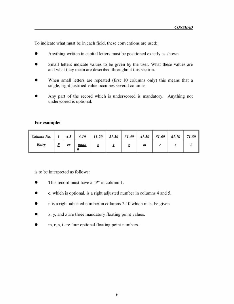
To indicate what must be in each field, these conventions are used:
Anything written in capital letters must be positioned exactly as shown.
Small letters indicate values to be given by the user. What these values are
and what they mean are described throughout this section.
When small letters are repeated (first 10 columns only) this means that a
single, right justified value occupies several columns.
Any part of the record which is underscored is mandatory. Anything not
underscored is optional.
For example:
Column No.
1
4-5
6-10
11-20
21-30
31-40
41-50
51-60
61-70
71-80
Entry
P
cc
nnnnn
x
y
z
m
r
s
t
is to be interpreted as follows:
This record must have a "P" in column 1.
c, which is optional, is a right adjusted number in columns 4 and 5.
n is a right adjusted number in columns 7-10 which must be given.
x, y, and z are three mandatory floating point values.
m, r, s, t are four optional floating point numbers.

7
4.1.1.2 GEOMETRY INPUT DATA FILE [.GEO]
This section of the CONSHAD input describes the geometric math model (GMM)
from which view areas or shadow tables are being created. CONSHAD is concerned
with surfaces involved in diffuse radiative heat exchange, and for reasons of
analytical simplicity and computational speed, only planar surfaces are allowed.
Computational simplicity further requires us to limit descriptive surfaces to
one-sided, covex polygons. One-sided means that only one face of the polygon is
considered to be involved in the radiation exchange. (To represent a thin plate
requires two polygons -- one for each side.) A convex polygon is one which has no
internal angle greater than 180 degrees. The GMM can be generated by a number of
different CAD packages, but the geometry data must be supplied to SSPTA in the
format described in this section.
Note: If GADS**
is used to develop the GMM, an SSPTA input file [*.GEO] which
contains the geometric math model data can be generated automatically, or by using
the Nastran to SSPTA conversion utility program.
Required Data Input
The first required record of every [.GEO] input file must be a TITLE
description. The title can be a maximum of 80-characters in length and
will appear on all output generated by the program.
The second required record (or list of records) is a description of the
GMM and is presented in the following sections.
The third and final required record of the geometry data input is an
"E" record. When the user has stored all of the geometry in the
CONSHAD geometry input file [*.GEO], this "E" record must be the
final record present in the [*.GEO] file to mark the end of the
geometry data.
End of Geometric Data Column No.
1
Entry
E
* = rootname of geometry file (e.g., DEMO)
** = GADS is an OPENGL Windows program used to develop
SSPTA (.GEO) Geometric Math Models (GMM). In addition,
Nastran Bulk Data files can be easily converted to SSPTA
(.GEO) files.

8
CONSHAD
Geometric Math Model Description Curvilinear and non-planar surfaces are represented in CONSHAD as several
polygons (facets) approximating the surface. A polygon, or surface, is defined by
first giving the vertexes of the surfaces Point records, then connecting the points
using a Surface record. The vertexes (points) are connected in order around the
surface, defining the active side of the surface by the right hand rule, i.e., the active
side of a surface faces an observer when the points are given in a counterclockwise
direction. There is implicitly defined in this geometry a right-handed Cartesian
coordinate system. All points are in this implicit coordinate system unless they are
specifically defined otherwise. These two types of card imagerecords, the Point
record and the Surface record, are the basis for the data input in this section. They are
augmented by other records allowing convenient local coordinate systems to be
constructed for defining points and allowing the user to give individual surfaces
special properties or specify special handling by the program. A surface generator is
also included which will create sets of Point and Surface records automatically to
approximate rectilinear or spherical shapes in a model.
The input to this section is conducted in two phases by the program. During the first
phase, the data records are read in and acted upon immediately by the program.
Surfaces are stored on an internal scratch file as they are encountered. When all the
data records have been read in, the program rewinds the scratch file, and during the
second phase, rereads the surfaces, sorts them by area (sorted order table can be
printed), and stores them in the program's main storage area. This is important to
note because some of the input records described below do not take effect until the
second phase of the input as noted in their description.
Geometry data input is terminated by an "E" record. When the user has stored all of
the geometry in the CONSHAD geometry input file [*.GEO], this "E" record must
still be present in the control input stream to mark the end of this section and the
beginning of the last input section, the run request section.
Point Definition Column No.
1
4-5
6-10
11-20
21-30
31-40
41-50
51-60
61-70
71-80
Entry
P
cc
nnnn
n
x1
y1
z1
m
x2
y2
z2
A point numbered "n" is defined at (x1,y1,z1) in the previously defined coordinate
system numbered "c". The program refers to the coordinate system "c" in order to
interpret (x1,y1,z1). If "c" is not given or is zero, the basic, implicit Cartesian
coordinate system is used. A second point, numbered "m", at (x2,y2,z2) can be
included on the same record. ( NOTE: While "m" is interpreted internally as an
integer by the program, it can be entered as either floating point, whole number or a
right justified integer in field 5. "n" and "m" are in the same "c" coordinate system).
9
CONSHAD
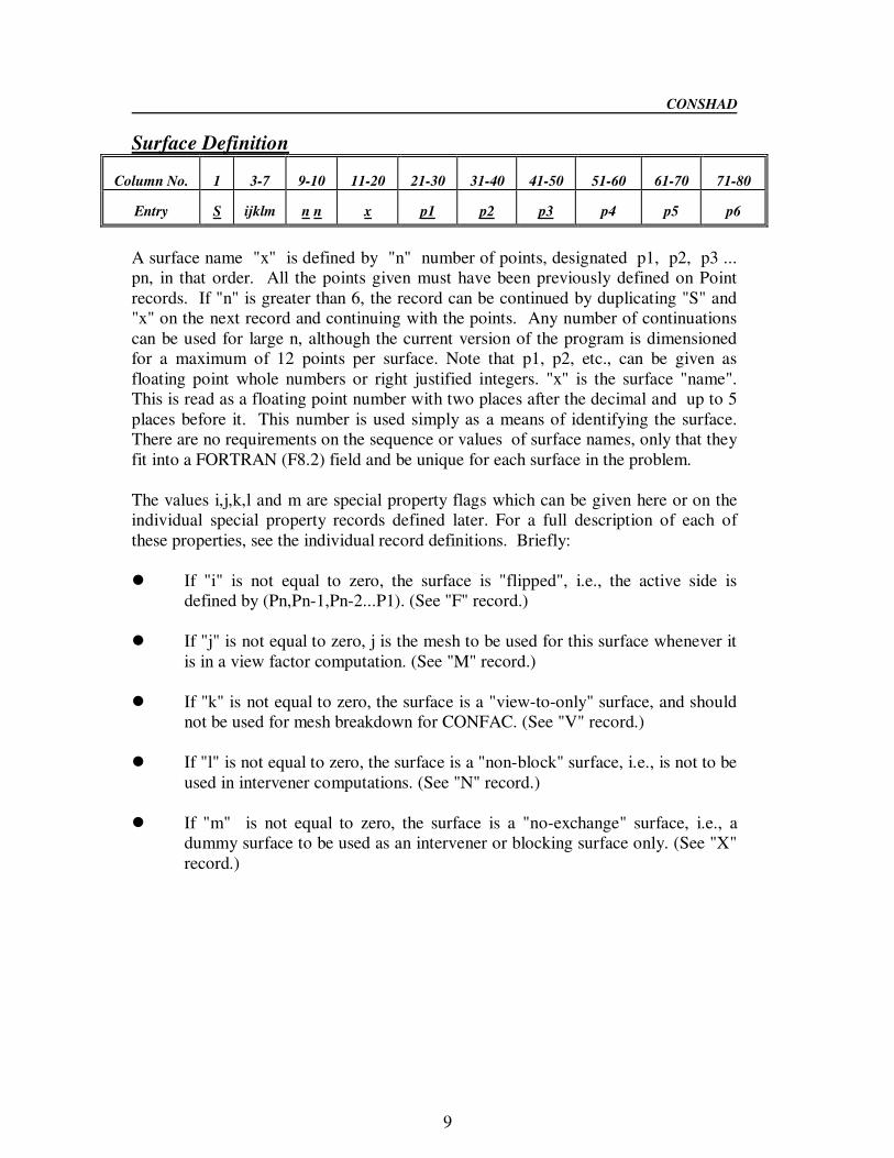
Surface Definition Column No.
1
3-7
9-10
11-20
21-30
31-40
41-50
51-60
61-70
71-80
Entry
S
ijklm
n n
x
p1
p2
p3
p4
p5
p6
A surface name "x" is defined by "n" number of points, designated p1, p2, p3 ...
pn, in that order. All the points given must have been previously defined on Point
records. If "n" is greater than 6, the record can be continued by duplicating "S" and
"x" on the next record and continuing with the points. Any number of continuations
can be used for large n, although the current version of the program is dimensioned
for a maximum of 12 points per surface. Note that p1, p2, etc., can be given as
floating point whole numbers or right justified integers. "x" is the surface "name".
This is read as a floating point number with two places after the decimal and up to 5
places before it. This number is used simply as a means of identifying the surface.
There are no requirements on the sequence or values of surface names, only that they
fit into a FORTRAN (F8.2) field and be unique for each surface in the problem.
The values i,j,k,l and m are special property flags which can be given here or on the
individual special property records defined later. For a full description of each of
these properties, see the individual record definitions. Briefly:
If "i" is not equal to zero, the surface is "flipped", i.e., the active side is
defined by (Pn,Pn-1,Pn-2...P1). (See "F" record.)
If "j" is not equal to zero, j is the mesh to be used for this surface whenever it
is in a view factor computation. (See "M" record.)
If "k" is not equal to zero, the surface is a "view-to-only" surface, and should
not be used for mesh breakdown for CONFAC. (See "V" record.)
If "l" is not equal to zero, the surface is a "non-block" surface, i.e., is not to be
used in intervener computations. (See "N" record.)
If "m" is not equal to zero, the surface is a "no-exchange" surface, i.e., a
dummy surface to be used as an intervener or blocking surface only. (See "X"
record.)

10
CONSHAD
Sample SSPTA [.GEO] Input File
SSPTA DEMO Geometry Data --> 1 SQ.FT. CUBE
P 1 12.0000 0.0000 0.0000
P 2 12.0000 12.0000 0.0000
P 3 12.0000 0.0000 12.0000
P 4 12.0000 12.0000 12.0000
P 5 0.0000 0.0000 0.0000
P 6 0.0000 0.0000 12.0000
P 7 0.0000 12.0000 0.0000
P 8 0.0000 12.0000 12.0000
S 4 1.00 1 2 4
3
S 4 2.00 5 6 8
7
S 4 3.00 6 3 4
8
S 4 4.00 5 7 2
1
S 4 5.00 2 7 8
4
S 4 6.00 5 1 3
6
E
Geometric Math Model

11

12
CONSHAD
Optional Data Input
Point Clearing Column No.
1
Entry
U
A "U" record undefines or clears all previously defined points from the programs' storage
area, making the point numbers available for reuse. This record has no effect on surfaces
or coordinate transformations defined before the record is given.
Spacing the Output Column No.
1
Entry
A single blank " " record will cause two blank lines to be printed when the record is
encountered.
Delete a Surface Column No.
1
9-10
11-20
21-30
31-40
41-50
51-60
61-70
71-80
Entry
D
a
b
c
d
e
f
g
This record caues the program to Delete surfaces previously defined with the names a, b,
c , d, e, f, and g. This data takes effect in the second input phase of the geometry section.
The "D" record is useful in removing part of a large model without disturbing the rest of
the data deck, for example, to remove a side of a box.
Reverse Active Side Column No.
1
9-10
11-20
21-30
31-40
41-50
51-60
61-70
71-80
Entry
F
a
b
c
d
e
f
g
The Flip record causes the reverse side of surfaces a,b,c,d,e,f,g to be made the active side.
This data takes effect in the second input phase.

13
CONSHAD
MESH -- View Factor Accuracy Column No.
1
9-10
11-20
21-30
31-40
41-50
51-60
61-70
71-80
Entry
M
n n
a
b
c
d
e
f
g
Surfaces a, b, c, d, e, f, g are assigned the special Mesh "n". Whenever a surface has a
special mesh assigned to it in this manner, the mesh "n" is used in all view area
computations involving the surface. In addition, the surface with the special mesh is
chosen as the surface to be subdivided. (See Appendix B for further description of this
mesh).
This is meaningful for CONFAC runs only. This record overrides the values on the
MESH record in the [.CON] input file only for the surfaces named.
No blockage Column No.
1
9-10
11-20
21-30
31-40
41-50
51-60
61-70
71-80
Entry
N
a
b
c
d
e
f
g
The surface name a, b, c, d, e, f, and g cannot "block", i.e., they are not to participate in
intervener computations.
No Exchange Column No.
1
9-10
11-20
21-30
31-40
41-50
51-60
61-70
71-80
Entry
X
a
b
c
d
e
f
g
This record specifies that surfaces named a, b, c, d, e, f, and g are dummy surfaces, to be
used as blockers or interveners in the computations but for which no view factors or
shadow tables will be generated. The intent of this record is to allow the user to create a
few large surfaces for the program to use in intervener computations. Typically a single
"X" surface is created which coincides with several smaller surfaces. The smaller
surfaces are given the "N" option. This way the program uses a single large surface in
the place of several smaller ones when doing intevener computations. No surface
specified with the "X" option will appear in the output.
View-to-only Column No.
1
9-10
11-20
21-30
31-40
41-50
51-60
61-70
71-80
Entry
V
a
b
c
d
e
f
g
The "V" record tells CONSHAD to use the other surface for mesh subdividing whenever
the surfaces named a, b, c, d, e, f, or g occur in a view factor computation with another
surface. This record can be used in such a way to avoid contour integrations that would
not yield accurate view factors.

14

15
CONSHAD
Coordinate Systems and Transformations
Column No.
1
2-5
9-10
11-20
21-30
31-40
41-50
51-60
61-70
Entry
C
mmst
n n
u
v
w
a
b
c
A coordinate system denoted by a "C" in column 1 and numbered "n" is defined, as
follows:
"s" and "t" give the type of coordinate system and are used to interpret the three coordinates given for any point which refers to this coordinate system. (See Point
record.) The following values have been implemented:
s = 0 or blank means that angles are in degrees.
s = 1 means that angles are in radians "s" is meaningful for t = 2 or 3, below.
t = 1 the (x,y,z) coordinates of points in the system are Cartesian coordinates. t = 2 the (x,y,z) coordinates are to be interpreted as (r,Θ,z) in a cylindrical coordinate
system. Θ is measured in the x-y plane from the x axis. Θ is degrees or radians
according to "s".
t = 3 the (x,y,z) coordinates of points in this system are to be interpreted as (p,φ,Θ) in
a sperical coordinate system; φ is measured from the z axis, and Θ is measured in the x-y plane from the x axis φ an dΘ are degrees or radians according to "s".
(u,v,w) and (a,b,c) are the rotations and translations, respectively, necessary to locate this
local coordinate system in the overall, implicit Cartesian coordinate system.
"m" is a special case, described below, which can be ignored for the moment.
The values (u,v,w) are degrees of rotation about the x,y, and z axes, respectively, of the
implicit coordinate system and (a,b,c) is the translation on the x,y, and z axes of the
implicit system, which locate this local coordinate system in the implicit one.

16
CONSHAD
These rotations and translations are all with respect to the unchanging, implicit
coordinate system. The local coordinate system should be seen as initially coinciding
with the implicit one. Each rotation and translation moves the local coordinate system
about in the implicit one. The user is, in effect, describing the motions required to take
the local system from its initial location and move it into some new position in the
implicit system, as though the local system were an object which could be so
manipulated. Rotations are applied sequentially about the three axes (x,y,z) and then
followed by translations along the same three axes. (CCW being positive.)
If (u,v,w) and (a,b,c) are all zero, the local system will coincide with the implicit system.
The "C" record does not have to be given when no special local coordinate system
different from the implicit system is needed.
When "m" is not zero, the record describes a chaining of coordinate systems. "m" is the
number of another coordinate system to which "n" is now linked. Points which refer to
coordinate system "m" will be treated as usual, then the new coordinates from that
transformation are further transformed by this new description "n". Thus it becomes
possible to describe an instrument in the cargo bay or in a spacecraft using a chained
coordinate system.
Several aspects of this use of coordinate system records should be noted:
Point records may reference coordinate system "n" directly, as usual. In so doing,
the points in no way become involved with the coordinate system "m".
The parameters "s" and "t" do not affect points in coordinate system "m". They
are used only for points referenced "n" directly.
Coordinate system "n" may itself be the subject of a coordinate system chaining.
This would affect both "n" and "m".
If "n" is a coordinate system number, only one other coordinate record may refer
to it at a time. If a second reference is made to "n", the second reference will
replace any other and a message is printed by the program to that effect. This
replacement will break any longer chain to "n" which may have existed through
the earlier references to "n". The program currently handles a total of 30

17
coordinate system records.
CONSHAD
Surface Generator
Column
1
2-8
9-10
11-20
21-30
31-40
41-50
51-60
61-70
Entry 1
G
aijklm
c c
name
α1
α2
α3
α4
α5
Entry 2
+
rs t nn
m m
u
v
w
x
y
z
An additional feature of CONSHAD is the capability to automatically generate surface
data by specifying a simple shape such as a sphere, cone, cylinder, or parts thereof, or a
rectilinear solid. This feature allows the user to specify all or part of a geometric model
using standard shapes. These shapes are generated in one of the coordinate systems
shown in Figure 4.2. The user describes the desired shape in its own coordinate system
of another geometric model, for example, an instrument. This model can further be
transformed into another coordinate system (for example, shuttle coordinate system)
which represents the complete geometric model to be used to generate view factors
and/or shadow tables.
Some of the standard shapes that can be defined in CONSHAD are curved surfaces.
CONSHAD does not have the ability to model curved surfaces directly; so faceted
surfaces are generated to represent the curved surfaces (spheres and cylinders), described
below.
a = 1 rectilinear solid = 2 cylinder (a cone can be generated by setting α1 or α2 to zero).
= 3 sphere
i,j,k,l,m = surface flags as on Surface record
cc = coordinate system number as on Point record
name = primary name of solid. Only the integer portion will
be used. Generated surfaces will be name.01, name.02, etc.
α1 - α5 = description parameters of the shape (See Figure
4.2)
r =0 --> no bottom cap, sphere or cylinder
=1 --> bottom cap, sphere or cylinder
s =0 --> no top cap, sphere or cylinder =1 --> top cap, sphere or cylinder
t =0 --> alpha angles given in degrees
=1 --> alpha angles given in radians
u, v, w = rotations in degrees and
x, y, z = linear translations. These values are used to locate
the figure in a local coordinate system which can further be oriented
with the "cc" coordinate system transformation.
nn, mm = number of surfaces to be generated in each

18
direction (for curved surfaces).

19
CONSHAD

20
CONSHAD
The generator works by creating Point and Surface records for the shape desired. These
Point and Surface records appear in the printed output and are interpreted in the usual
way by CONSHAD.
A "U" record to clear all previously defined points is also created by the surface generator
and is placed just before the generated points and surfaces. For this reason, Generator
inputs may not be interposed between other Point inputs and the Surfaces based on them.
Generator records must appear before or after such sequences.
In the case of a generated sphere, when α2 is greater than zero degrees or alpha3 is less
than 180 degrees, the program will leave the corresponding end of the sphere open unless
"r" or "s" is specified for closure of the -Z and +Z ends respectively. When α2 is 0
degrees or α3 is 180 degrees, the closure for that end is ignored.
It may be desirable in some cases to refer to specific surfaces generated by the "G"
record. The generated surface names can be predicted. The integer portion of the "name"
field is used as a base name, and the first surface generated is named : base.01 . The
others are base.02, base.03, etc. The sequence of surfaces generated for the rectilinear
solid is:
+X
+Y
+Z
-X
-Y
-Z
.01
.02
.03
.04
.05
.06
For the cylinder and sphere, the sequence of surfaces starts at the +Z end of the figure and
goes around from α4 to α5 for "mm" number of surfaces. If "nn" is greater than 1, the
next band towards -Z is generated for "mm" more surfaces. When the body of the figure
is generated, and when closure of the figure is required, the program then generates "mm"
number of triangular closure surfaces form α4 to α5 at the +Z end. Following taht , the -Z
closure is generated, if required, in the same way.
All solids are generated as exterior figures, with the active sides facing out. If an interior
figure is desired, the "i" field can be set to 1 and all surfaces will be "flipped" as
described earlier for the "i" field of the Surface record.

21
CONSHAD
Sample Surface Generator Input Record
Column
1
2-8
9-10
11-20
21-30
31-40
41-50
51-60
61-70
Entry 1
G
2
3
11.00
3.0
6.0
10.0
0.0
180.0
Entry 2
+
11
2 4
90.0
6.0
CONSHAD will generate a set of surfaces like those in Figure 4.3. Figure 4.3 (a) shows
the shape desired; Figure 4.3 (b) shows the surfaces generated by CONSHAD; and Figure
4.3 (c) shows the final position of the generated surfaces in the coordinate system.
Note: The final figure has 16 surfaces as a result of the surface breakdown selected (i.e.,
2 along the z-axis, 4 about the z-axis, plus 4 on each end).

22
CONSHAD
4.1.1.2 CONSHAD INPUT DATA FILES [.CON], [.CVW], [.CSH]
This first section of input tells CONSHAD what kind of run is being made and what
options are to be used during the run. Both types of CONSHAD runs, CONFAC and
SHADOW, have different types of run request records. Therefore, to provide the option
of selecting either CONFAC or SHADOW in a batch type environment, three input files
are needed. The [.CVW] file contains the view area (i.e., view factor, shape factor, etc.)
run request records and the [.CSH] file contains the shadow table run request records.
Before executing CONSHAD, either the [.CVW] or the [.CSH] file must be copied into
the [.CON] file, which is needed by the program CONSHAD for execution.
Required Data Input
The first required record of every CONSHAD run must be a TITLE
description. The title can be a maximum of 80-characters in length and
will appear on all output generated by the program.
The second required record for a CONSHAD run must be one of the
following two records: 1) CONFAC 2) SHADOW
1) CONFAC [.CVW]
Column
1
2
3
4
5
6
Entry
C
O
N
F
A
C
CONFAC computes the view areas for the geometric math model.
2) SHADOW [.CSH]
Column
1
2
3
4
5-6
11-20
21-30
31-40
41-50
51-60
61-70
Entry
S
H
A
D
OW
λ1
λ2
λ3
v1
v2
v3
SHADOW computes the shadow tables for the geometric math model. v1, v2, v3 are the
beginning, ending, and increment values, respectively, for the NU (v) angles of the
shadow tables. λ1, λ2, λ3 are the beginning, ending , and increment values, respectively,
for the LAMDA (λ) angles of the shadow tables.
Defaults are: λ1, λ2, λ3 = 0., 360., 15.
v1, v2, v3 = 0., 180., 15.

23
CONSHAD
The third required record tells the program to begin reading geometry
data starting with the record after the DATA record.
Data Record Column No.
1
2
3
4
10
Entry
D
A
T
A
n
"n" is right justified in column 10 and defines the engineering units of the input
data to CONSHAD. "n" may have one of the following values:
1 - inches
2 - feet
3 - centimeters
4 - meters
Based on the specified value of "n" the program will choose output units as
follows:
a) If input is in inches or centimeters, output will be in centimeters.
b) If input is in feet or meters, output will be in meters.
The units chosen for output will be automatically carried through the
computations of ORBITAL, SCRIPTF and ABSORB.
Optional Data Input
Other record control options for which defaults are provided need only be given when
other than the default values are desired.
The following records are optional. When used, they invoke special features of the
program or override program default values. This record can be placed anywhere
between the TITLE record and DATA record.
View Factor Accuracy Parameter Column No.
1
2
3
4
7-10
Entry
M
E
S
H
nnnn
This record sets the mesh size used in the CONFAC integration technique. The default
value is 2. If "n" is given, "n" is the mesh used for all surfaces not otherwise defined with
a special mesh ( see SURFACE record). The MESH record has no effect on SHADOW
runs.

24
CONSHAD
LET Option Column No.
1
2
3
Entry
L
E
T
Normally, the CONSHAD program will stop for errors detected in the data rather than
proceed into computation with bad data. The LET option allows the program to proceed
despite data errors. However, when the LET option is given, the program may
subsequently fail or compute incorrectly.
NOBLOK Option Column No.
1
2
3
4
5
6
Entry
N
O
B
L
O
K
For CONFAC and SHADOW runs, NOBLOK option considers no blocking
(intervening computation) is to be done. All view factors and shadow tables will be
computed as though there were no intervening surfaces.
PRINT Option Column No.
1
2
3
4
5
8-10
Entry
P
R
I
N
T
lmn
The values l, m, and n control the amount of printout generated as follows:
View areas computed during CONFAC operation:
l = 0 do not print l = 1 print view factors and areas for each surface (default)
l = 2 print view factors sums only
Developed and sorted geometry (second input phase):
m = 0 do not print m = 1 print surface areas and normals (default)
m = 2 print surface coordinates, area and normals
Individual geometry data records (input records):
n = 0 do not print
n > 0 print (default)
Tables computed during SHADOW operation:
l = 0 do not print
l = 1 print condensed tables (default)
l = 2 print tables in long form
25
CONSHAD
NOHOL Option Column No.
1
2
3
4
5
Entry
N
O
H
O
L
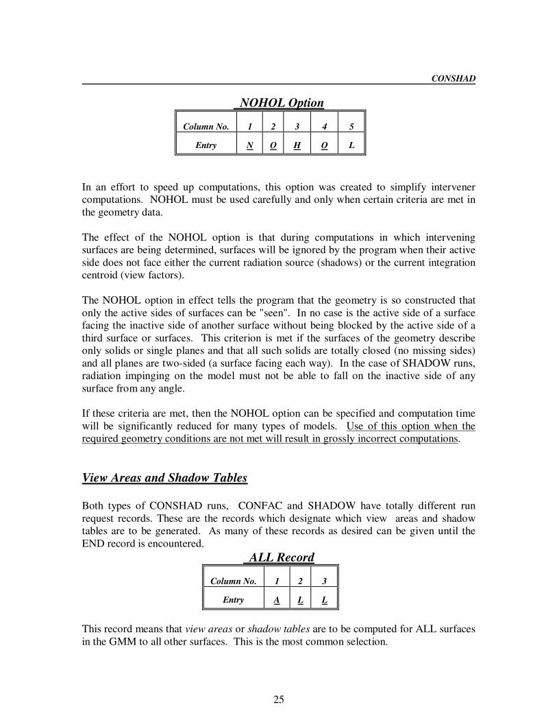
In an effort to speed up computations, this option was created to simplify intervener
computations. NOHOL must be used carefully and only when certain criteria are met in
the geometry data.
The effect of the NOHOL option is that during computations in which intervening
surfaces are being determined, surfaces will be ignored by the program when their active
side does not face either the current radiation source (shadows) or the current integration
centroid (view factors).
The NOHOL option in effect tells the program that the geometry is so constructed that
only the active sides of surfaces can be "seen". In no case is the active side of a surface
facing the inactive side of another surface without being blocked by the active side of a
third surface or surfaces. This criterion is met if the surfaces of the geometry describe
only solids or single planes and that all such solids are totally closed (no missing sides)
and all planes are two-sided (a surface facing each way). In the case of SHADOW runs,
radiation impinging on the model must not be able to fall on the inactive side of any
surface from any angle.
If these criteria are met, then the NOHOL option can be specified and computation time
will be significantly reduced for many types of models. Use of this option when the
required geometry conditions are not met will result in grossly incorrect computations.
View Areas and Shadow Tables
Both types of CONSHAD runs, CONFAC and SHADOW have totally different run
request records. These are the records which designate which view areas and shadow
tables are to be generated. As many of these records as desired can be given until the
END record is encountered.
ALL Record Column No.
1
2
3
Entry
A
L
L
This record means that view areas or shadow tables are to be computed for ALL surfaces
in the GMM to all other surfaces. This is the most common selection.

26
CONSHAD
Specified Range Calculations Column No.
1
2
3
4
5
11-20
21-30
Entry
R
A
N
G
E
a
b
Two options are available: 1) "a" can be given alone.
2) "a" and "b" can both be given.
1) If only "a" is given, the program computes view areas or shadow tables from the surface named
"a" to all other surfaces.
2) If "a" and "b" are given, the program computes all view areas or shadow tables for all surfaces
whose surface name is a number >= a and <= b, i.e., all surface names in the range "a" to "b".
CONFAC Only
Specific View Area Calculations Column No.
1
2
3
4
5
6
11-20
21-30
Entry
F
A
C
T
O
R
a
b
The program is to compute a view area only between surfaces "a" and "b".
SHADOW Only
Specific Shadow Table Calculations Column
1
2
3
4
5
11-20
21-30
31-40
41-50
51-60
61-70
71-80
Entry
T
A
B
L
E
a
b
c
d
e
f
g
Shadow tables for surfaces with names a,b,c,d,e,f, and g only will be computed.
END Record Column No.
1
2
3
Entry
E
N
D
When th END record is given, the program ends computations and outputs the results of
the CONFAC run in the [.OVW], and [.FAC] output files and the SHADOW run in the
[.OSH] and [.SHA] output files. If the END record is given without any other, the
program will stop.
Note: File Manager takes care of format restrictions automatically. The user does not
need to be concerned with format restrictions when using File Manager to
generate input files.

27
CONSHAD
4.1.2 CONSHAD OUTPUT DATA
4.1.2.1 Output Data From CONSHAD [.OVW], [.OSH]
CONSHAD will write all program status and error messages to the CONSHAD output
file [*.OVW] and [.OSH]. These file(s) will also display the beginning and ending times,
and the date of the CONSHAD run.
4.1.2.2 View Factor Output Data [.FAC]
The program writes the result of a run to the [.FAC] file in an 80 column format. An
effort has been made to keep the output compact, since many numbers can be generated.
The [.FAC] output file consists of a title, a table containing surface names and other
information, and a list of computed view factors.
The following describes the output:
TITLE (20A4)
The title of the run which produced this output.
N, IUNIT (2I5)
The number of surfaces and the engineering units of the model.
KEY1, NAME1, AREA1, KEY2, NAME2, AREA2, KEY3, NAME3,AREA3
The sorted surface key (see Appendix B), the surface name and the surface area,
are given three per record until all surfaces have been given.
K, N, J1, F1, J2, F2 . . . Jn, Fn
This record contains N view factors F1, F2...Fn from the surface whose sorted key
is K to the surfaces whose sorted keys are J1, J2...Jn. The view factor in each
case is the view factor for the smaller surface. CONSHAD actually computes the
black body, radiative view area coupling between two surfaces. In order to keep
the output compact, the program outputs the view factor from the smaller surface
(numerically a larger factor) which is a number from zero to one. The view area
can be computed by multiplying the view factor times the area of the smaller
surface.
See the sample problem for an example of this output.

28
CONSHAD
4.1.2.3 SHADOW Output Data [.SHA]
The program writes the computed shadow tables (actually visible fraction tables) to the
[.SHA] file in an 80 column format. The output consists of a title, a list of surface
descriptions, a record describing the tables, and the tables themselves.
TITLE (20A4)
The title of the run which produced this output.
N, IUNIT (2I5)
The number of surfaces and the engineering units of the model.
I, KEY, NAME, AREA, X, Y, Z
The name sorted number I, the are-sorted KEY, the surface NAME, the surface
AREA, and the direction cosines X, Y, and Z of the surface normal (facing
direction). One record for each surface.
STARTNU, ENDNU, STEPNU, STARLAM, ENDLAM, STEPLAM
The start, end, and step angles (in degrees) for the tables produced in this run.
These values are copied from the SHADOW record of the prolog section of the
input.
TABLE VALUES
The shadow tables incorporate a special data compacting scheme. The values in a table,
which range form 0.0 to 1.0 are converted to integers form 0 to 900, proportionately.
They are then written out in fields of FORTRAN format I3 where the following values
are used in a scheme to compact tables.
0 to 900 A table value in the range 0.0 to 1.0,
proportionately.
-1 to -98 A repetition factor, indicating that a value is
to be repeated from 1 to 98 times.
-99 End of table.
901 to 999 Reserved for future use.
Using these definitions, the tables are written as a continuous list of numbers, row after
row, using a repetition factor wherever possible to indicate that a value in the table is
repeated, instead of writing the value itself that many times.

29
CONSHAD
A simple example, a small (4 x 4) table might be handled as follows:
1. 1. 1. 1.
.9 .8 .8 .8
.8 .2 .2 .1
0 0 0 0
Would be converted to this:
900 900 900 900
810 720 720 720
720 180 180 90
0 0 0 0
Then to this:
900 900 900 900 810 720 720 720 720 180 180 90 0 0 0 0
Then to this using repetition factors:
900 -3 810 720 -3 180 -1 90 0 -3 -99
This last row is what would be written out to the [.SHA] output file, 25 values to a
record. The format used is (25I3, I3, I2) where the last 2 values are the table number and
record sequence number.
From this output the tables can be easily reconstructed.
See the sample problem for an example of this output.

30
WORKSHEETWORKSHEETWORKSHEETWORKSHEET
4.2 WORKSHEET
WORKSHEET is a utility subroutine whose sole purpose is to aid in the preparation of
optical property and node number assignments for surfaces which are input to SCRIPTF,
the SSPTA subprogram which logically follows WORKSHEET.
4.2.1 INPUT DATA TO WORKSHEET
4.2.1.1 WORKSHEET Input Data from CONSHAD Output [.FAC]
Required Input
There are two forms of input to the WORKSHEET program. The first is an AF type data
file [.FAC], output by CONSHAD, containing the names, areas and sorted keys of the
model being prepared.
4.2.1.2 WORKSHEET Input Data [.WRK]
Optional Input The second form of input to WORKSHEET is optional and is a WORKSHEET type data
file [.WRK], containing optical property and node number assignments in the format
described below.
TITLE (20A4)
NAME, NODE, ALPHA, EMISS (F10.0, I5, 2F5.0)
NOTE: The user should refer to the section of the SCRIPTF program for a
detailed description of the forms that optical property input may take.
Any number of separate inputs may be given. Inputs of this form do not need to contain
a record for every surface, although WORKSHEET [.WKS] output file must contain a
record for every surface. The program may be used in a few different ways. If run with
only an AF type input, the output will be a "worksheet" printout with fill-in spaces for
property and node assignments. The WORKSHEET [*.WKS] file could then be edited
to insert the property and node numbers. The information shown here is a smaple of the
fill-in printout:
Record No.
1-10
11-15
16-20
21-25
1
WORKSHEET -- DEMO.WRK
2
1.00
N
A
E
3
2.00
N
A
E

31
4 3.00 N A E

32
WORKSHEET
If the program is run with a complete set of optical property and node assignments, the
[.SHT] output file will be a printout showing all the assigned values and the
WORKSHEET [.WKS] data file generated will be ready to be input to the SCRIPTF
program. ALPHA and EMISS optical property data are rounded to three decimal places
by the program with 0.001 to 0.999 being the smallest and largest values used.
Input Value
Program Value
.024
0.024
.025
0.025
.026
0.026
.999
0.999
.002
0.002
*** Note: SCRIPTF program will abort if ALPHA or EMISS are 0.00 ***
If the program is run with some of the necessary optical properties and assignments
missing, the output file [.WKS] will consist of a printout showing user assigned values
where they are given and N, A, or E designations where values are missing. This output
data file can be renamed to [.WRK] and used as input to the WORKSHEET program in
later runs.
4.2.2 WORKSHEET OUTPUT DATA
4.2.2.1 Output File From WORKSHEET [.WKS], [.SHT]
The WORKSHEET [.WKS] file will contain the surface number, node number,
absorptivity, emmissivity values for each surface and the view area for each surface
which is needed by the SCRIPTF program to compute radiation ASCRIPF values.
WORKSHEET will write all program status and error messages to the WORKSHEET
output file [.SHT]. This file will also display the beginning and ending times, and the
date of the WORKSHEET run.

33
SCRIPTFSCRIPTFSCRIPTFSCRIPTF
4.3 SCRIPTF The SCRIPTF program uses the black body view areas computed by CONSHAD, based
on the planar surfaces geometric model and the optical properties prepared by
WORKSHEET, to create two sets of simultaneous equations. The sets of equations
represent the diffuse radiative interchange of the geometric model in the IR and UV
wavelengths. The solution to the set of equations for the IR wavelengths
is used, along with surface-to-node assignments, to compute the diffuse radiative
couplings for nodes in a thermal model. These couplings are output by the program in
the [.RAD] output file as ASCRIPTF type data and are used as input for TAK-II and
SINDA. Additionally, the solutions to both sets of equations are preserved for the
program ABSORB, to be used in computing absorbed environmental fluxes. These
solutions are output by the program as IRINVERS in the [.IR] data output file, and
UVINVERS in the [.UV] data output file.
To compute the inverse matrix set of simultaneous linear equations in SCRIPTF usually
requires a large amount of memory. SCRIPTF uses the Choleski square root method of
matrix inversion and special storage techniques to perform the matrix inversion in a small
amount of memory. Very large, symmetric matrices can be inverted by the program.
When generating the radiative couplings for nodes in a thermal model, there will be cases
in which the user wishes to assign couplings to space. SCRIPTF has provisions for
creating a "space" node and assigning radiative couplings to it from other nodes. This is
done by computing the sum of all radiative couplings for each node and assigning a
coupling to "space" equal to the difference between that sum and the total radiative area
of the node. This technique can be used to create a node and couplings for any
unmodeled, uniform environment.
Note: Caution must be used in developing the geometric math
model (GMM) in CONSHAD. The geometric model must satisfy the
NOHOL condition described in CONSHAD. If it does not,
couplings to the space node will be unrealistically high. A potential
problem to be avoided is to ensure that any surface having a view-
to-space not be blocked by the non-active side of any other surfaces.
This results in a larger view-to-space from the other surfaces due to
the missing (not computed) view area to the non-active side of the
blocking surfaces.

34

35
SCRIPTF Several other important considerations to be understood when using a space node are:
the space node must be highest node number in the system.
missing or lost view factors will be assigned to space when you have a space
node.
The maximum number of surfaces that SCRIPTF can handle is 2000.
4.3.1 INPUT DATA TO SCRIPTF
Input files needed by SCRIPTF include the following:
TITLE, run parameters and property data [.SCF]
Node and optical property assignments [.WKS]
Black body view areas [.FAC]
SCRIPTF has additional features allowing the user to define fixed temperature nodes and
to change the optical properties of groups of related surfaces. These features are
described in the sections that follow.

36
SCRIPTF
4.3.1.1 SCRIPTF Input Data [.SCF]
Title and Run Parameters:
TITLE (20A4)
M, ISPACE, CUTOFF, FCUT, ESP (2I5,3F5.0)
where,
M is the number of surfaces in the CONFAC run.
ISPACE is the space node number.
< 0 create a space node numbered ISPACE.
= 0 do not create a space node.
> 0 create a space node numbered one larger than the largest
node number in the model.
Note: If ISPACE .NE. 0 , then self-view areas are assigned to the space node, if
ISPACE .EQ. 0 , then self-view areas are retained as self-views.
CUTOFF is the cutoff limit for ASCRIPTF couplings computed for TTA
and SINDA. (All values less than CUTOFF are discarded).
FCUT is the cutoff limit for blackbody view factors (all values
less than FCUT are discarded and are not included in the matrix.
This option should be used carefully as severe errors could occur
in ABSORB if too many factors are eliminated. SCRIPTF prints a
warning message if more than 10 % of the view factors from any
one surface are discarded using this option.
ESP is the emissivity of the space node. (default = .999)
Property Data:
There are three records which may be input here. All of them have the same form.
Column No.
1-3
6-10
11-20
21-30
31-40
41-50
51-60
61-70
71-80
Entry
Knn
a e
v2
v3
v4
v5
v6
v7
v8
The records are interpreted according to K which may be an A, E, or an * (asterisk).

37
SCRIPTF If K = A, then ae is the absorptivity to be assigned to all surfaces with a group nn
given in the WORKSHEET [*.WKS] input field for the absorptivity. Also,
surfaces named v1, v2...etc., will be given an absorptivity equal to ae. If nn is
omitted (i.e., left blank) only surfaces v1, v2 ... will be affected. If v1, v2 ... are
left blank, only the group nn absorptivities will be affected.
If K = E, then ae is an emissivity value to be assigned in the same manner as the
absorptivities above, to all surfaces with group = nn and to surfaces v1, v2,...etc.
If K = *, then property data entry has ended.
Examples of Property Data Input:
Column No.
1-3
6-10
11-30
21-30
31-40
41-50
51-60
61-70
71-80
Entry
A 2
0.15
14.03
14.04
SCRIPTF will assign the value of .15 as the solar absorptivity to all surfaces in "group 2"
and to surfaces 14.03 and 14.04.
Column No.
1-3
7-10
11-30
21-30
31-40
41-50
51-60
61-70
71-80
Entry
E 2
0.75
22.01
22.02
22.08
22.10
SCRIPTF will assign the value of .75 as the IR emissivity to surfaces 22.01, 22.02, 22.08,
and 22.10. (There is no "group" input).
Column No.
1
Entry
*
An * (astersisk) denotes the "End of the Property Data" input.
Note: The first record in the SCRIPTF [.SCF] data file must be a
TITLE record as described, and the last record must be an *
(asterisk), even if no property data was entered.

38
SCRIPTF
4.3.1.2 SCRIPTF Input Data from WORKSHEET Output [.WKS]
This input to SCRIPTF is generated by WORKSHEET and read in by SCRIPTF with the
following format:
SNAME, ND, AL, EM, ARX, KEY (F10.0, I5, 2F5.0, E15.8, I5)
Exactly one record must be included for every surface in the geometric math model
(GMM), where:
SNAME is the surface name in the GMM.
ND is the node number to which the surface is assigned.
AL is the solar absorptivity assigned to the surface.
EM is the IR emissivity assigned to the surface.
ARX is the surface area in the GMM.
KEY is the area-sorted key in the GMM.
SNAME, ARX and KEY are provided automatically by the WORKSHEET program.
Node assignments must be provided in this section for every surface if radiative
couplings are to be output. Optical properties may be given here or in the property data
section of SCRIPTF or partially in both sections. At the end of the property section, the
program will stop if optical properties have not been provided for every surface.
The values AL and EM can be given in a special form in order to define groups of
surfaces which the user might wish to manipulate together. Normally, solar absorptivity
and emisssivity are numbers less than one. If AL or EM is given as a number greater
than one in the WORKSHEET [.WRK] file, the program will interpret the integer part on
the number as a group number. In the property data section of SCRIPTF the user can
assign a single optical property to all surfaces with the same group number. The
fractional part of the AL or EM value will be treated as a default value for the optical
property when no group value is assigned in the property data.
Optical properties are then input as, N.xx where N is the (optional) group number for this
property and .xx is the optical property to be used when no group input value is given.
As an example, if a surface were given AL = 1.04 and EM = 2.15, then with no further
input in the property data section, the surface would be assigned AL = .04 and EM = .15.
If the property data section gave a value for group 1 absorptivities of .5, then the surface
would have AL = .5 and EM = .15. Group 1 emissivity is not affected by group 1
absorptivity; the two are completely seperate.
Optical properties may be given as the integer part (group) only, the fraction part
(property) only, or both. When one record has been read for every surface the input ends.

39
SCRIPTF
4.3.1.3 SCRIPTF Input Data from CONSHAD Output [.FAC]
The SCRIPTF [.FAC] input file contains the AF type data output from CONSHAD.
4.3.2 SCRIPTF OUTPUT DATA
4.3.2.1 Output Data from SCRIPTF [.ASF]
SCRIPTF will write all program status and error messages to the SCRIPTF output file
[.ASF]. This file will also display the beginning and ending times, and the date of the
SCRIPTF run.
4.3.2.2 IR INVERSE MATRIX Output Data [.IR]
Stored SCRIPTF property IR data which is used by ABSORB.
4.3.2.3 UV INVERSE MATRIX Output Data [.UV]
Stored SCRIPTF property UV data which is used by ABSORB.

40
ORBITALORBITALORBITALORBITAL
4.4 ORBITAL The subprogram ORBITAL computes the flux intensities incident on each surface of a
geometric model of a spacecraft. The program ABSORB subsequently computes the
absorbed power which results from these incident fluxes, taking into account multiple
diffuse reflections.
There are two sources of external heat flux which are considered in a spacecraft energy
balance: the sun and nearby planets. The emission from nearby planets is considered to
be in the infrared spectrum and diffuse in nature. The input from the sun comprises two
forms. The first is power radiated directly from the sun to the spacecraft. This power is
in the form of a nearly collimated beam with a spectral content ranging from the
ultraviolet to the infrared wavelengths. The second form is power emitted by the sun and
reflected by a nearby planet onto the spacecraft. This reflected sunlight has the same
spectral content as direct solar flux and is assumed to be diffusely reflected by the planet.
The subprogram ORBITAL provides a tool with which one can calculate the
environmental heat flux incident on a spacecraft in orbit about either the Earth or Earth's
moon. In subsequent discussions, the term Earth should be interpreted as the planetary
body about which the spacecraft is orbiting.
The program calculates incident flux from each of the sources listed above. Specifically,
it calculates direct solar flux, earth emission and solar flux reflected by the earth. These
fluxes are used to calculate absorbed powers for use in computing the spacecraft energy
balance. A detailed discussion of the numerical methods used by ORBITAL can be
found in Appendix C.
An important aspect of ORBITAL is the program's ability to use stored tables of shadow
factors computed by the subprogram CONSHAD in calculating incident fluxes. This is
discussed in Section 4.4.1. ORBITAL calculates heat fluxes using a spacecraft model
comprising planar surfaces defined by an area and surface normal. The spacecraft may
be modelled in any orbit about either the Earth or the Earth's moon. In addition, the
spacecraft may be either three-axis stabilized, pointing toward the earth, the sun, a star, or
spin stabilized about any arbitrary axis. The relative orientations of surfaces are
permitted to change at each computation step so that variable geometry problems can be
handled; for example, an earth oriented spacecraft with a solar oriented solar array can be
modeled.
The program calculates the times of both entry into and exit from the Earth eclipse.
During the period of eclipse, no direct or reflected solar flux is incident on the spacecraft.

41
ORBITAL The orbit or spacecraft attitude can be changed at any point in the analysis so that a
trajectory problem (such as a launch or orbit transfer trajectory) may be handled. See
option ITRAJ.
An added feature of the subprogram ORBITAL is the ability to show the position of
Earth and Sun relative to the shuttle model (see Appendix D). This is done in three
orthographic printer plots of the shuttle model (X-Y, X-Z, and Y-Z). In each view, the
relative locations of the Sun and Earth in that plane are indicated by the letters S and E
respectively. If both the sun and earth should be in the same direction in any view (i.e.,
both along the X-axis) the letter B is printed in the appropriate location. See option
IPLOT and Figure 4.4.
4.4.1 INPUT DATA TO ORBITAL
4.4.1.1 ORBITAL Input Data from CONSHAD Output [.SHA]
ORBITAL uses the shadow tables generated by CONSHAD in calculating incident
fluxes. The shadow factors take into account the shadows cast on each surface in the
geometric model by other surfaces for the different directions of arriving environmental
fluxes.

42
ORBITAL
4.4.1.2 REQUIRED CONTROL INPUT [.ORB]
(1) TITLE (20A4) The first record of every ORBITAL run must be a title. The title will appear on
output generated by the program.
(2) N, IBTUW, ISS, IBLOK, IPRNT, ITRAJ, ISPIN, IGEOM, IPLOT, IHHX
(10I5)
This record sets a series of program swithches which determine what type of run
this will be.
N is the number of surfaces in the spacecraft geometric
model.
IBTUW specifies the unit of power to be printed on the output. This does
not affect the computation of the incident fluxes which is done in
watts.
= 0 power in watts
= 1 power in Btu/hr
= 2 power in Btu/min
ISS specifies the frequency for outputting fluxes onto the [.QE]
and [.QSA] data files and hence specifies what power data will be
available to the thermal math model.
= 0 output fluxes for each step in the orbit
> 1 output only the orbital average fluxes
IBLOK designates whether shadow tables will be used in computing
incident fluxes. If shadow tables are not being used, see Special
Inputs after this section.
= 0 shadow factor (visible fraction) tables are provided in the
form of a SHADOW type data set on the inputlist.
> 0 do not account for shadowing (no tables)
IPRNT specifies the frequency for printing fluxes. When ISS is > 0, only
the orbital averaged fluxes will be printed. When ISS is = 0, then
the fluxes at aeach orbital step are printed or not according to this
parameter.
= 0 print output for each step in orbit
> 0 print output for orbit averaged fluxes only
ITRAJ designates whether the run is simulating a single orbit computation
or a trajectory (changing orbit). See Special Inputs section to
describe a trajectory.

43
ORBITAL
ISPIN designates whether the spacecraft is stationary or is spinning about some
axis as it proceeds throught the orbit.
= 0 fixed spacecraft
> 0 multiple orbit computations are made with incremental
steps of rotation (spin) being specified by successive ATT1,
ATT2, or ATT3 values (Line 5 of [.GEO] file). See Special
Inputs section for full description of a spinning spacecraft.
IGEOM designates whether there is a fixed or changing geometry
throughout the orbit. See Special Inputs section for a description of
changing geometry.
= 0 fixed geometry (1 set of shadow tables)
> 0 changing geometry -- shadow tables "must" be provided for
each user designated computational step in the orbit. Care
must be taken to ensure that the shadow tables are
prepared in correct order to correspond with the sequential
positions in orbit.
IPLOT specifies whether the user wants a printer plot of the relative
position of the sun and earth with respect to the shuttle cargo bay
model.
= 0 no plot
> 0 plot at each position in orbit even if printout of fluxes is not
requested (IPRNT>0).
IHHX was added by Henry Hartley of NASA/GSFC in 1987 to
specify whether the user wants a printed output of the direction
cosines for the geometric model.
= 0 (or blank) not printed
> 0 direction cosines are printed to the output file [.FLX].
IUNIT was added to allow the user to specify orbit altitude in kilometers
(Km) or meters (m) and the solar, earth IR constants in [W/(m*m)]
The default is the standard input which is altitude in nautical miles
(nm) and environmental constants in [Btu/(hr-ft*ft)].
= 0 (or blank) default values
= 1 altitude in kilometers (km) solar, and earth IR constants in
[W/(m*m)]
= 2 altitude in meters (m) solar, and earth IR constants in
[W/(m*m)]

44
ORBITAL
(3) M, NSUN, NMOON, NOR, NSH, NAPRX, NRMIN, ISRNG1 (16I5)
This record contains a number of parameters which determine the computational
procedure and accuracy of the orbital flux calculations desired.
M specifies the attitude control mode of the spacecraft. There
are three attitude modes available in the program.
= 1 spacecraft is earth-oriented; X, Y, and Z are aligned with
earth oreiented axis r, w, and i respectively.
= 2 not currently used.
= 3 spacecraft is inertially fixed; X, Y, and Z are aligned with
the celestial coordinate system, X2, Y2, and Z2.
= 4 spacecraft is solar oriented ; X, Y and Z are aligned with
solar oriented axis X2, Y2, and Z2.
NSUN specifies whether the effect of the earth's orbital eccentricity on the solar
constant is to be accounted for.
= 0 program used the specified solar constant
> 0 program computes effect of earth's elliptical orbit on solar
constant.
NMOON specifies whether or not the spacecraft or not the spacecraft is
orbiting around the moon. This has the effect of changing radius,
gravitational constant, and I.R. radiation constant to values
representative of the moon.
= 0 Earth orbit
< 0 lunar orbit
NOR specifies the number of orbital revolutions to be accounted
for before beginning the orbit for which flux computations are
desired. Parameters that are used in the program to compute the
regression of the nodes fixed in the program.

45
ORBITAL
NSH specifies number of times user specified computational step
size is to be halved in determining the orbital position at which the
satellite enters or leaves the Earth's shadow.
= integer number of halvings desired (e.g., NSH = 5)
NAPRX designates computational scheme for earth and albedo fluxes (see
Apppendix C).
= 0 approximate method is used (no shadowing effects are
modelled)
> 0 numerical integration of visible portion of Earth is used
NRMIN specifies the first estimate of the number of integration rings to be
used for dividing the visible cap of the earth ( See Appendix C) not
used when NAPRX = 0.
= integer number of rings (e.g., NRMIN = 6)
ISRNG1 specifies the first estimate of the angular width of each integration
ring corresponding to the number of specified integration rings
(NRMIN) (refer to Appendix C).
= integer value for angular ring width (degrees) measured
from the spacecraft to the center fo the visible cap
(e.g., ISRNG1 = 10)
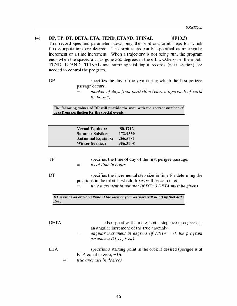
46
ORBITAL
(4) DP, TP, DT, DETA, ETA, TEND, ETAND, TFINAL (8F10.3)
This record specifies parameters describing the orbit and orbit steps for which
flux computations are desired. The orbit steps can be specified as an angular
increment or a time increment. When a trajectory is not being run, the program
ends when the spacecraft has gone 360 degrees in the orbit. Otherwise, the inputs
TEND, ETAND, TFINAL and some special input records (next section) are
needed to control the program.
DP specifies the day of the year during which the first perigee
passage occurs.
= number of days from perihelion (closest approach of earth
to the sun)
TP specifies the time of day of the first perigee passage.
= local time in hours
DT specifies the incremental step size in time for determing the
positions in the orbit at which fluxes will be computed.
= time increment in minutes (if DT=0,DETA must be given)
DETA also specifies the incremental step size in degrees as
an angular increment of the true anomaly.
= angular increment in degrees (if DETA = 0, the program
assumes a DT is given).
ETA specifies a starting point in the orbit if desired (perigee is at
ETA equal to zero, = 0).
= true anomaly in degrees
The following values of DP will provide the user with the correct number of
days from perihelion for the special events.
Vernal Equinox: 80.1712
Summer Solstice: 172.9530
Autumnal Equinox: 266.5981
Winter Solstice: 356.3908
DT must be an exact multiple of the orbit or your answers will be off by that delta
time.
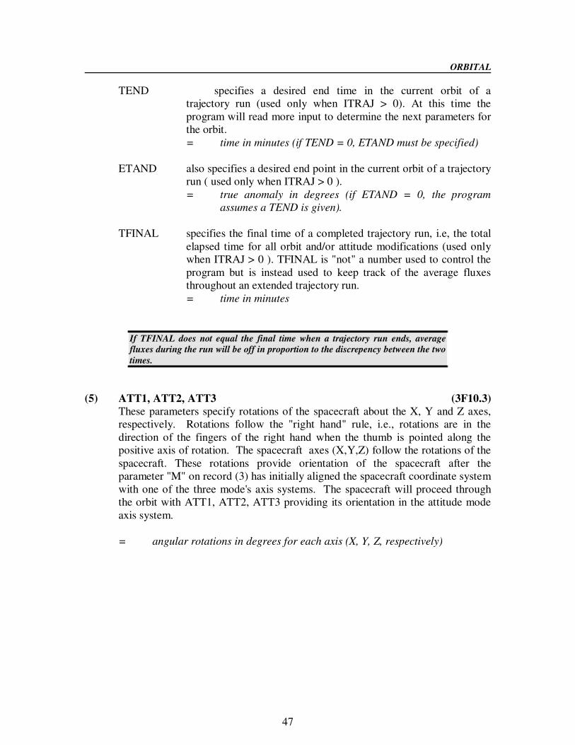
47
ORBITAL
TEND specifies a desired end time in the current orbit of a
trajectory run (used only when ITRAJ > 0). At this time the
program will read more input to determine the next parameters for
the orbit.
= time in minutes (if TEND = 0, ETAND must be specified)
ETAND also specifies a desired end point in the current orbit of a trajectory
run ( used only when ITRAJ > 0 ).
= true anomaly in degrees (if ETAND = 0, the program
assumes a TEND is given).
TFINAL specifies the final time of a completed trajectory run, i.e, the total
elapsed time for all orbit and/or attitude modifications (used only
when ITRAJ > 0 ). TFINAL is "not" a number used to control the
program but is instead used to keep track of the average fluxes
throughout an extended trajectory run.
= time in minutes
(5) ATT1, ATT2, ATT3 (3F10.3)
These parameters specify rotations of the spacecraft about the X, Y and Z axes,
respectively. Rotations follow the "right hand" rule, i.e., rotations are in the
direction of the fingers of the right hand when the thumb is pointed along the
positive axis of rotation. The spacecraft axes (X,Y,Z) follow the rotations of the
spacecraft. These rotations provide orientation of the spacecraft after the
parameter "M" on record (3) has initially aligned the spacecraft coordinate system
with one of the three mode's axis systems. The spacecraft will proceed through
the orbit with ATT1, ATT2, ATT3 providing its orientation in the attitude mode
axis system.
= angular rotations in degrees for each axis (X, Y, Z, respectively)
If TFINAL does not equal the final time when a trajectory run ends, average
fluxes during the run will be off in proportion to the discrepency between the two
times.

48
ORBITAL
(6) SOLC, ALB, ERTHE (3F10.3)
This record specifies the radiation constants used to compute incident flux
intensities. See record (2) for allowable units.
SOLC specifies the solar constant in Btu/(hr-sqft). When NSUN =
0 (fixed solar constant), this value is left unchanged for all orbital
positions. When NSUN > 0 , SOLC is taken as the solar
constant at the semi-major axis of the Earth's orbit and the solar
constant for specific orbital positions at the specified time of year
is then computed appropriately.
ALB specifies the albedo of the Earth.
ERTHE specifies the Earth IR emission in Btu/(hr-sqft). If the value is not
given, it is computed from SOLC and ALB by:
(1-ALB) * SOLC
ERTHE = ------------------------------
4
(7) HP, YINC, ECC, YLATP, YLONP, ENS (6F10.3)
This record specifies orbital parameters and the direction of motion of the
satellite.
HP specifies the altitude of perigee
= in nautical miles, if IUNIT=0. (default)
= in kilometers, if IUNIT =1.
= in meters, if IUNIT=2.
YINC specifies the angle of inclination of the orbit plane to the
Earth's equator in degrees.
ECC specifies the orbit eccentricity.
YLATP specifies the latitude of the sub-perigee point in degrees form the
equator.
YLONP specifies the longitude of the sub-perigee point in degrees from
Greenwhich.
ENS specifies the direction of satellite motion along the orbit
path
= + 1 satellite is travelling North at perigee
= - 1 satellite is travelling South at perigee

49
ORBITAL
4.4.1.3 SPECIAL INPUTS
Four of the input parameters on record (2) imply further input as described below.
IBLOK - When IBLOK is set to 0, meaning that shadow tables are provided,
SSPTA assumes that the geometric description of the model is being transferred
to ORBITAL as part of the SHADOW tables. The tables contain, as they come
from CONSHAD, a header with the name, area and facing direction of each
surface. When IBLOK is set greater than 0, meaning no shadow tables are
provided, the user must supply the geometric model description, and place it in
the control deck immediately following record 2. There must be exactly N (first
parameter on record 2) records describing the model, one for each surface, as
follows:
(2a) NODE, NTAB, AREA, ALP, EPS, A, B, G, CMNT (215,6F10.3,2X,A8)
NODE = an integer value which serves as a surface identifer
NTAB = a shadow table number. Should be zero for this application
AREA = surface area in square feet (ft2)
ALP = solar absorptance of the surface
EPA = I.R. emissivity of the surface
A,B,G = the direction cosines of the surface normal with respect to the spacecraft
coordinate system (XB, YB, ZB, respectively)
CMNT = an alphanumberic name that may be given for this surface
ITRAJ - when ITRAJ is set greater than 0, the program will compute fluxes for
the orbit described in records 3 through 7, as usual. At the end of the orbit, the
program will read the following additional record to determine how to proceed.
(8) IA, M, ATT1,ATT2,ATT3, DT, DETA, TEND, ETAND (215,7F10.3)
IA is the only new parameter on this record and designates the type of change in
orbit and/or attitude that is being described by the parameters that follow.
= -1 signifies the end of a trajectory run (the remaining parameters on the record need not be
specified). This must be the last record for a trajectory run.
= 0 signifies a change in the attitude mode (M) and the orientation angles (ATT1, ATT2,
ATT3) of the spacecraft in the next position of the current orbit. The current orbit is then
continued to the new end in the new step increments.
= 1 signifies the beginning of new orbit parameters (the remaining parameters on this record
need not be specified). Another set of the required input records 3 through 7 must follow
this record in the input sequence. The program will compute fluxes for the new orbit at
the current time in the trajectory run. TFINAL (record 4) is not updated but is held at its
initial value.
More than one of these records may be given for a trajectory run. This record
follows record (7) of the normal required record input.

50
ORBITAL
M gives the attitude mode as described on record (3). ATT1, ATT2, ATT3
specify spacecraft rotations as described on record (5). DT, DETA, TEND,
ETAND specifiy orbit steps as described on record (4).
ISPIN - When ISPIN is set greater than 0, the program will repeat the orbit
described by the usual input as many times as desired. For each repeition (after
the first regular orbit) the program will read one additional input record
representing an increment of spin angles. The record is as follows:
(8) ATT1, ATT2, ATT3 (3F10.3)
These are the three rotation parameters from input record (5). They are changed
internally to the new values and the original orbit is re-run with the new
spacecraft rotations. The values of ATT1, ATT2, ATT3 specify the next position
in a regular series of incremental steps of spin of the spacecraft. This process is
repeated, reading another input record with each orbit repetition until an input
record is read having ATT1>360; then the program ends. The spinning spacecraft
is effectively modelled in the next SSPTA step when the user invokes the
ABSORB program. ABSORB reads the multiple-orbit output from this program
and averages the incident fluxes at each orbit position across all the orbit
repetitions (one for each spin increment). Absorbed power is computed for a
single orbit using the spin-averaged fluxes.
While the program does not check the successive values of ATT1, ATT2, and
ATT3, they should constitute a regular incremental spin of the spacecraft since
ABSORB will average the resultant fluxes without regard to angle.
IGEOM - when IGEOM is greater than 0, a geometric model with changing
geometry can be analyzed, i.e., a spacecraft which has moving external parts, a
separate CONSHAD run must be made for each spacecraft configuration desired,
corresponding to the configuration of each orbit position used in ORBITAL. The
resultant shadow tables must be combined in the [.SHA] data file in the correct
sequence, and therefore, will be included in the ORBITAL inputlist as the
SHADOW data. ORBITAL will read a new full set of shadow tables each time a
new orbital position increment (DT or DETA) is made. Thus the first set of
shadow tables in the file is used for computations of incident flux at the first orbit
position, the second set of shadow tables is used at the second orbit position, etc.
A title is the first record of each new full set of shadow tables. When ORBITAL
interjects an extra orbit position at an earth shadow crossing, the set of shadow
tables nearest the crossing is used twice and the synchrony of shadow tables vs.
orbit position is not lost.
Note: The parameters ITRAJ, ISPIN, and IGEOM cannot be given in combination with
each other, the program is currently limited to handling these features one at a
time.

51
ORBITAL
4.4.1.4 SAMPLE INPUT SEQUENCES
1-
5
6-
10
11-
15
16-
20
21-
25
26-
30
31-
35
36-
40
41-
45
46-
50
51-
55
56-
60
61-
65
66-
70
71-
75
76-
80
1
TITLE
2
N
A
B
C
D
E
F
G
H
I
3
M
J
K
L
O
P
Q
R
4
DP
TP
DT
DETA
ETA
TEND
ETAND
TFINAL
5
ATT1
ATT2
ATT3
6
SOLC
ALB
ERTHE
7
HP
YINC
ECC
YLATP
YLONP
ENS
Simple Orbital Run
Record No. Description
(1) TITLE
(2) N, A=IBTUW, B=ISS, C=IBLOK, D=IPRNT, E=ITRAJ, F=ISPIN, G=IGEOM, H=IHHX,
I=IUNIT
(3) M, J=NSUN, K=NMOON, L=NOR, O=NSH, P=NAPRX, Q=NRMIN, R=ISRNG
(4) DP, TP, DT, DETA, ETA, TEND, ETAND, TFINAL
(5) ATT1, ATT2, ATT3
(6) SOLC, ALB, ERTHE
(7) HP, YINC, ECC, YLATP, YLONP, ENS
Run with No Shadowing
Record No. Description
(1) TITLE
(2) N, IBTUW, ISS, IBLOK, (>0), IPRNT, ITRAJ (-0), IGEOM (-0)
(2a) NODE(1), NTAB(1), AREA(1), ALP(1), EPS(1), A(1), B(1), G(1), CMNT(1)
.
.
.
.
.
.
(2a) NODE(N), NTAB(N), AREA(N), ALP(N), EPS(N), A(N), B(N), G(N), CMNT(N)
(3) M, NSUN, NMOON, NOR (=1), NSH, NAPRX, NRMIN, ISRNG1
(4) DP, TP, DT, DETA, ETA, TEND (=0), ETAND (=0), TFINAL (=0)
(5) ATT1, ATT2, ATT3
(6) SOLC, ALB, ERTHE
(7) HP, YINC, ECC, YLATP, YLONP, ENS

52
ORBITAL
Trajectory Run
Record No. Description (1) TITLE
(2) N, IBTUW, ISS, IBLOK (=0), IPRNT, ITRAJ (>1), ISPIN (=0),
IGEOM (=0)
(3) M, NSUN, NMOON, NOR (=1), NSH, NAPRX, NRMIN, ISRNG1
(4) DP, TP, DT, DETA, ETA, TEND, ETAND, TFINAL
(5) ATT1, ATT2, ATT3
(6) SOLC, ALB, ERTHE
(7) HP, YINC, ECC, YLATP, YLONP, ENS
(8) IA (=0), M, ATT1, ATT2, ATT3, DT, DETA, TEND, ETAND
If on RECORD (8), IA (=1), then
(3) M, NSUN, NMOON, NOR (=1), NSH, NAPRX, NRMIN, ISRNG1
(4) DP, TP, DT, DETA, ETA, TEND, ETAND
(5) ATT1, ATT2, ATT3
(6) SOLC, ALB, ERTHE
(7) HP, YINC, ECC, YLATP, YLONP, ENS
(8) IA (=-1), ends trajectory run
Spinning Spacecraft Run
Record No. Description
(1) TITLE
(2) N, IBTUW, ISS, IBLOK (-0), IPRNT, ITRAJ (=0), ISPIN (>0),
IGEOM (=0)
(3) M, NSUN, NMOON, NOR (=1), NSH, NAPRX, NRMIN, ISRGN1
(4) DP, TP, DT, DETA, ETA, TEND (=0), ETAND (=0), TFINAL (=0)
(5) ATT1, ATT2, ATT3
.
.
.
. ATT1 (>360)
Changing Geometry Run
Record No. Description
(1) TITLE
(2) N, IBTUW, ISS, IBLOK (=0), IPRNT, ITRAJ (=0), ISPIN (-0),
IGEOM (>0)
(3) M, NSUN, NMOON, NOR (1), NSH, NAPRX, NRMIN, ISRNG1
(4) DP, TP, DT, DETA, ETA, TEND (=0), ETAND (=0), TFINAL (=0)
(5) ATT1, ATT2, ATT3 (6) SOLC, ALB, ERTHE
(7) HP, YINC, ECC, YLATP, YLONP, ENS
Read shadow tables from inputlist
.
.
.
Read shadow tables from inputlist

53
ORBITAL There are six "orbital elements" which are used to describe a spacecraft orbit. Figure 4.5
represents a geocentric orbit and the orbital elements. The three "orientation" elements are
described as:
Ω, longitude of the ascending node, measured in the plane of the equator from the
direction of the vernal equinox to the direction of the ascending node (intersection
of the orbit with the equator) -- for heliocentric orbits substitute "ecliptic" for
"equator".
i, the inclination, the angle between the plane of the orbit and the plane of the
equator.
ω, the argument of perigee, or angle, in the plane of the satellites's orbit, between the
ascending node and perigee -- "perihelion" for heliocentric orbits.
The remaining three elements are the "dimensional" elements and are described as:
a, the semimajor axis or mean distance.
e, the eccentricity, or the ratio of the distance from the center of the orbit to the
focus (the center of the earth) to the mean distance.
T, the time of perigee passage.
Currently, the orbits in SSPTA are defined using non-standard terms, such as the "time" for
crossing the equatorial plane instead of the longitude of the ascending node and the Sun location
is defined by the "day of year" instead of the right ascention and declination of the Sun. The
modifications made by Analytix Corporation to the VAX version of SSPTA have now been

54
added to the PC version of SSPTA.
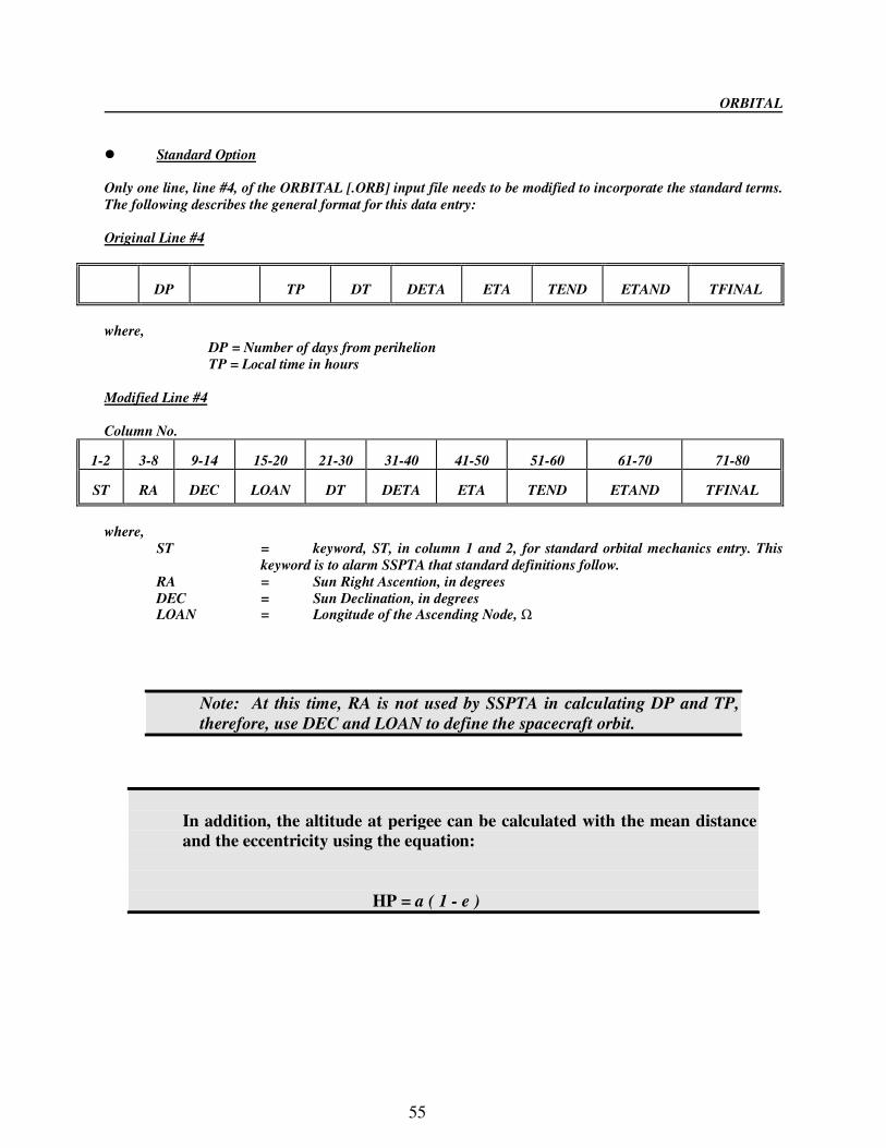
55
ORBITAL
Standard Option
Only one line, line #4, of the ORBITAL [.ORB] input file needs to be modified to incorporate the standard terms.
The following describes the general format for this data entry:
Original Line #4
DP
TP
DT
DETA
ETA
TEND
ETAND
TFINAL
where,
DP = Number of days from perihelion
TP = Local time in hours
Modified Line #4
Column No. 1-2
3-8
9-14
15-20
21-30
31-40
41-50
51-60
61-70
71-80
ST
RA
DEC
LOAN
DT
DETA
ETA
TEND
ETAND
TFINAL
where,
ST = keyword, ST, in column 1 and 2, for standard orbital mechanics entry. This
keyword is to alarm SSPTA that standard definitions follow.
RA = Sun Right Ascention, in degrees
DEC = Sun Declination, in degrees LOAN = Longitude of the Ascending Node, Ω
Note: At this time, RA is not used by SSPTA in calculating DP and TP,
therefore, use DEC and LOAN to define the spacecraft orbit.
In addition, the altitude at perigee can be calculated with the mean distance
and the eccentricity using the equation:
HP = a ( 1 - e )

56
ORBITAL
Beta Angle Option
Since most sensitivity and/or parametric studies are not performed for specific orbits or sun locations, but rather for a series of Beta Angles, and to maintain compatibility with TRASYS (Thermal Radiation Analysis System),
additional modifications have been added to the SSPTA subprogram ORBITAL. As described earlier, only Line
#4 of the ORBITAL [.ORB] control input file needs to be modified to use this option.
Original Line #4
DP
TP
DT
DETA
ETA
TEND
ETAND
TFINAL
where,
DP = Number of days from perihelion
TP = Local time in hours
Modified Line #4
Column No.
1-4
5-10
11-20
21-30
31-40
41-50
51-60
61-70
71-80
BETA
BANG
CANG
DT
DETA
ETA
TEND
ETAND
TFINAL
where,
BETA = keyword, BETA, in column 1 through 4, for alarming SSPTA that the input
contains Beta Angle definitions.
BANG = BETA Angle, angle in degrees measured from Zo (orbit normal) to the sun vector.
CANG = CIGMA Angle, angle in degrees measured from the periapsis point Xo
(perigee) to the sun vector.

57

58
ORBITAL
4.4.1.5 PRINTED OUTPUT
The first message that appears in the output is written by the subroutine NUREAD if shadow
tables are read (IBLOK = 0). The message indicates the title read with these tables and the
number of surfaces for which the shadow tables have been generated. This allows the user to
verify that the correct shadow tables have been read for the orbital run. This message does not
appear if no shadow tables are read (IBLOK >0).
The next block of output is an echo of the input. The following is a description of these
parameters as they appear in the output with reference to the corresponding parameter
described in the INPUT section of this manual:
MODE = attitude mode (M)
ALB = Earth's albedo factor (ALB) ERTHE = Earth's I.R. emittance (ERTHE)
SOLC = solar constant (SOLC)
NSUN = constant or varying solar constant (NSUN)
ECC = orbit eccentricity (ECC)
INC = orbit inclination (YINC)
LATP = latitude at perigee (YLATP)
LONG = longitude at perigee (YLONP)
RP = orbit altitude at perigee (HP)
DP = day of the year (DP)
TP = time of the day at perigee (TP)
DT = orbit time step size (if specified) (DT)
DETA = orbit angular step size (if specified) (DETA) ATT1,2,3 = space craft rotations (ATT1, ATT2, ATT3)
The above parameters are repeated at each change of orbit in a trajectory run (IA = 1) after the
fluxes for the orbital steps have been printed.
The next output is a summary of the input surfaces;
NODE = Surface number assignments are taken from the
shadow table data.
BTAB = shadow table number for this surface, if any. This
number is the sorted "key" from CONSHAD.
AREA = surface area in square feet
ABSORB = solar absorptivity of surface
EMIT = I.R. emissivity of surface
ALPHA,BETA,GAMMA = direction cosines of the surface normals
CMNT = surface name from CONSHAD when shadow tables have been read.

59
ORBITAL Whether the next block of output is printed depends on whether output is written for each step in
the orbit. If either ISS > 0 or IPRNT > 0, this block of output will not be printed.
The following is a description of the parameters that appear in each step in the orbit:
ETA = true anomoly of spacecraft in degrees
ORBIT = fraction of final orbit(s) completed at this position in orbit
ALT = altitude of spacecraft at this position in orbit measured in
nautical miles
TIME = time from the start of the orbit (trajectory in minutes
(IBTUW = 0 or 2) or hours (IBTUW = 1)
LAT = spacecraft latitude at this position
LON = spacecraft longitude at this position
RS,R = Sun-Earth-spacecraft angle
The following parameters for each surface appear in the same block of output:
Relative SURF No. = Sequential surface number listing
Actual SURF No. = Surface number from CONSHAD
Area = Surface Area in square feet
SOLAR = incident solar flux intensity in Btu/hr-ft2
ALBEDO = incident reflected solar albedo flux intensity in Btu/hr-ft2
EARTH IR = incident earth emitted flux intensity in Btu/hr-ft2
TOTAL = SOLAR + ALBEDO + EARTH IR
The last block of output is a compilation of the final averages for the orbit or trajectory. The
heading for this block is a statement of the percent of orbit that the spacecraft is in sunlight. The
parameters written for each surface are the same as those written at each step in the orbit.
The next two blocks of output (or the next block if either ISS>0 or IPRNT>0) are
repeated for each full orbit of a spinning spacecraft run (ISPIN > 0).
The last block of output displays the actual time of day that the run completed, the delta time of
the run in minutes (TFINAL - TSTART), and the date the run was made.

60
ORBITAL
4.4.1.6 PROGRAM NOTES
The shadowing taken into account by the program is determined by interpolation in tables of
visible fractions as a function of the incoming radiation angles. When desired, the user can
prepare such tables for every PLANAR surface in the model using the program CONSHAD.
The shadowing capability of the program ORBITAL has been designed to beused conveniently
in conjunction with the SHADOW option of the program CONSHAD.
A subroutine, NUREAD, is used to read the visible fraction ("shadow") tables and convert them
to a different but compact form for internal storage. A certain machine dependent technique is
employed in storing these tables and is necessary because of the large amount of computer
memory needed if the shadow tables are stored in a conventional way. Due to the use of this
technique, changing computers requires rewriting of both subroutines NUREAD and DINTK,
the interpolating subroutine.
The tables read by NUREAD are described in the CONSHAD section on shadow table output.
The compact form of tables is read and NUREAD further compacts the tables to
store them internally. The LOGICAL*1 and CHARACTER*8 byte concepts described must be
replaced with another if the program is to be used on another type of computer.
All tables are stored in memory in an eight byte CHARACTER variable named BLOFA. The
tables for a satellite configuration must all have the same dimensions; the same, equal angular
steps must be used for each row and the same, equal steps for the column entries. Row
increments need not equal column increments.
The tables are stored in the single, CHARACTER*8 variable and referenced by computing the
location of a desired entry, given the position of a table and the displacement of the
entry. An entry in a table is stored (and retrieved) using the following method:
If all tables are I columns (nu) and J rows (lambda), then the entry in row L, column K of
Table N is an array location: M = E + T where, E = the entry displacement in a table and T =
((N-1) o (I o J)), the table's beginning location in the list. If a shadow entry in a table is a value 0
to 1 (after decoding the compact input) then an eight bit representation of the entry is a value 0 to
1.
e = f * 128
where,
e = table entry value (integer, truncated)
f = visible fraction being stored (0 to 1).
A stored integer entry of 1 is equal to a visible fraction of 1/128 = 0.0078 which is, then,
the precision of the table values.

61
ORBITAL
4.4.2 ORBITAL OUTPUT DATA
4.4.2.1 OUTPUT file from ORBITAL [.FLX]
ORBITAL will write all program status and error messages to the ORBITAL output file [.FLX].
This file will also display the beginning and ending times, and the date of the ORBITAL run.
4.4.2.2 SOLAR AND ALBEDO FLUX OUTPUT DATA [.QSA]
UV flux data used by ABSORB to calculate environmental absorbed powers.
4.4.2.3 EARTH IR FLUX OUTPUT DATA [.QE]
IR flux data used by ABSORB to calculate environmental absorbed powers.

62
ABSORBABSORBABSORBABSORB 4.5 ABSORB
ABSORB computes the fluxes (UV and IR) absorbed on the surfaces defined in the geometric
math model (GMM) and assigns the resultant powers to nodes for the thermal math model. The
absorbed fluxes include those fluxes which are diffusely reflected from other surfaces in the
model. The output from ABSORB consists of absorbed power for each node in the model in a
format compatible with TTA and SINDA.
4.5.1 INPUT DATA TO ABSORB
4.5.1.1 ABSORB Input Data from SCRIPTF Data [.UV], [.IR]
The SCRIPTF input to ABSORB consists of the UVINVERS [.UV] and IRINVERS [.IR] data
files.
4.5.1.2 ABSORB Input Data from ORBITAL DATA [.QSA], [.QE]
The ORBITAL input to ABSORB consists of the incident UV flux [.QSA] and the incident IR
flux [.QE] data files.
4.5.2 ABSORB OUTPUT DATA
4.5.2.2 ABSORB Output Data [.ABS]
The absorbed energy for each node can also be found in the ABSORB output file [.ABS]. The
steady-state and/or transient data in this file can be converted to SINDA or TAK format using the
program ABS2SIN.
4.5.2.2 ABSORB Output Data [.POW]
ABSORB generates the energy absorbed on the surfaces defined in the geometric model and
assigns them to the nodes defined in WORKSHEET. The output is written to the [.POW] file.

63
Sample ProblemSample ProblemSample ProblemSample Problem Chapter 5Chapter 5Chapter 5Chapter 5 5.0 Sample Problem
5.1 GEOMETRIC MODEL GENERATION [.GEO]
1
6-
10
11-
15
16-
20
21-
25
26-
30
31-
35
36-
40
41-
45
46-
50
51-
55
56-
60
61-
65
66-
70
71-
75
76-
80
1
SSPTA Geometric Math Model -- DEMO.GEO
2
P
1
12.0000
0.0000
0.0000
3
P
2
12.0000
12.0000
0.0000
4
P
3
12.0000
0.0000
12.0000
5
P
4
12.0000
12.0000
12.0000
6
P
5
0.0000
0.0000
0.0000
7
P
6
0.0000
0.0000
12.0000
8
P
7
0.0000
12.0000
0.0000
9
P
8
0.0000
12.0000
12.0000
10
S
4
1.00
1
2
4
3
11
S
4
2.00
5
6
8
7
12
S
4
3.00
6
3
4
8
13
S
4
4.00
5
7
2
1
14
S
4
5.00
2
7
8
4
15
S
4
6.00
5
1
3
6
16
E
5.2 CONSHAD VIEW FACTORS - CONFAC [.CVW]
Record
1
2
3
4
5
6
7
8
9
10
1
DEMO CONFAC RUN -- DEMO.CVW
2
C
O
N
F
A
C
3
D
A
T
A
1
4
E
5
A
L
L
6
E
N
D

64
Sample Problem
5.3 CONSHAD BLOCKAGE TABLES - SHADOW [.CSH]
Record
1
2
3
4
5
6
7
8
9
10
1
DEMO SHADOW RUN -- DEMO.CSH
2
S
H
A
D
O
W
3
D
A
T
A
1
4
E
5
A
L
L
6
E
N
D
5.4 WORKSHEET Preparation for SCRIPTF-F [.WRK]
Record No.
1-10
11-15
16-20
21-25
1
WORKSHEET --
DEMO.WRK 2
1.00
1
1.00
1.00
3
2.00
2
1.00
1.00
4
3.00
3
1.00
1.00
5
4.00
4
1.00
1.00
6
5.00
5
1.00
1.00
7
6.00
6
1.00
1.00
5.5 SCRIPTF ASCRIPTF Couplings, UV and IR Matrix Inverses [.SCF]
Record No.
1
2-3
4-5
6-10
11-15
16-20
21-25
1
SCRIPTF -- DEMO.SCF
2
6
1
0.010
0.010
0.999
3
A
1
0.999
4
E
1
0.999
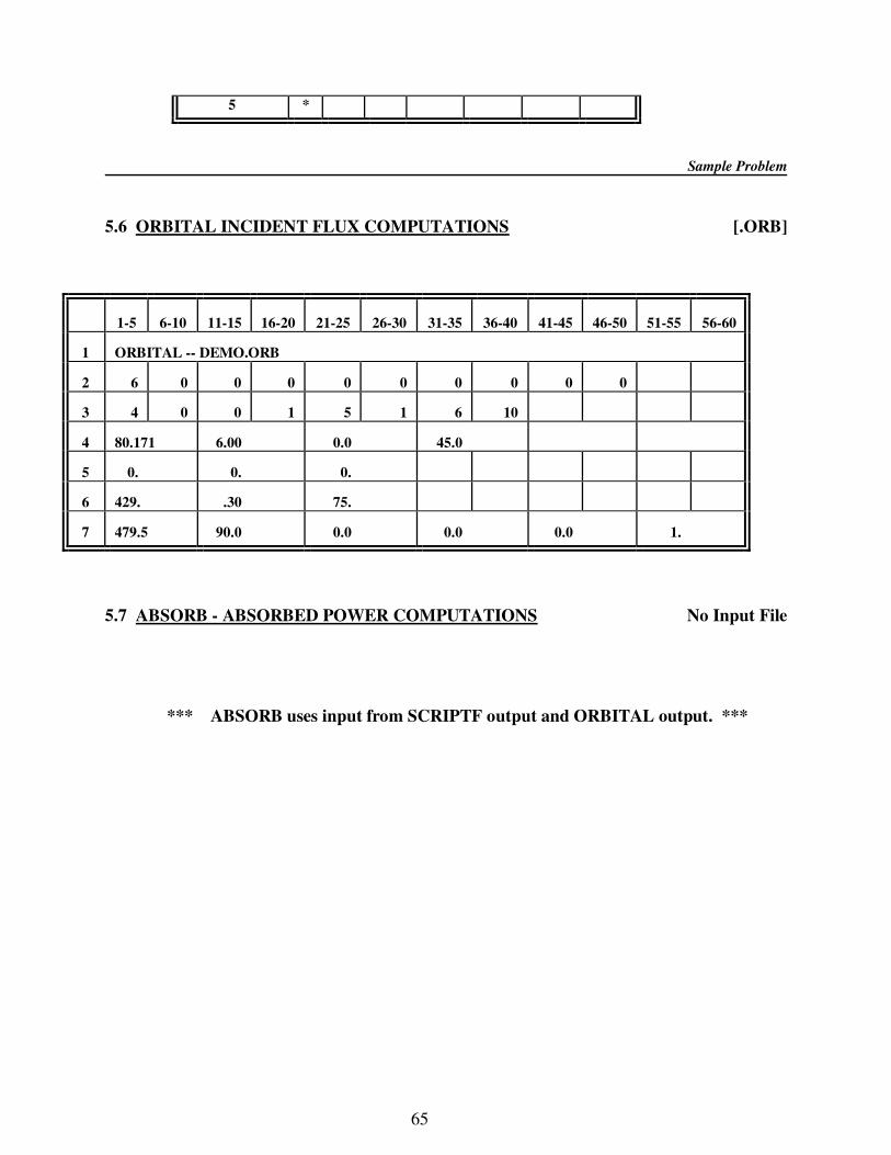
65
5 *
Sample Problem
5.6 ORBITAL INCIDENT FLUX COMPUTATIONS [.ORB]
1-5
6-10
11-15
16-20
21-25
26-30
31-35
36-40
41-45
46-50
51-55
56-60
1
ORBITAL -- DEMO.ORB
2
6
0
0
0
0
0
0
0
0
0
3
4
0
0
1
5
1
6
10
4
80.171
6.00
0.0
45.0
5
0.
0.
0.
6
429.
.30
75.
7
479.5
90.0
0.0
0.0
0.0
1.
5.7 ABSORB - ABSORBED POWER COMPUTATIONS No Input File
*** ABSORB uses input from SCRIPTF output and ORBITAL output. ***

66
67
Appendix AAppendix AAppendix AAppendix A Utility Programs
RAD2SIN Converts SSPTA [.RAD] output file containing
ASCRIPTF radiation couplings to TAK-II and SINDA
format.
ABS2SIN Converts SSPTA [.ABS] output file containing
steady-state absorbed powers to TAK and SINDA format.
Converts SSPTA [.ABS] output file containing
transient absorbed powers to SINDA and TAK format.
NAS2GEO Converts NASTRAN [.NAS] geometry file to SSPTA [.GEO] file.
GEO2NAS Converts SSPTA [.GEO] file to a NASTRAN [.NAS] file.