3Exotic Operators

The core of SQL language is fairly compact. Select-project-join, set operators, nested subqueries, inner views, aggregation – make up a very short but expressive list of operators. This is all that most users ever need for everyday usage. Once in a while, however, there comes a problem that can’t be solved by these means. Often, such a problem is evidence of a missing language feature.

User-defined aggregates and Pivot, which we study in the beginning of this chapter, are undoubtedly on top the list of the desired features. Next, Symmetric Difference and Logarithmic Histograms are two more query patterns that every developer sooner or later must encounter in their practice. Then, either Relational Division, or Skyline comes perhaps once in a lifetime. And, finally, the Outer Union is so rare, that there is almost no chance an (ordinary) developer would ever need it. Yet, we’ll get a chance to leverage it in the next chapter.

List AggregateList aggregate is not exactly a missing feature. It is implemented as a built-in operator in Sybase SQL Anywhere and MySQL. Given the original Emp relation

1

select deptno, ename from emp; DEPTNO ENAME 10 CLARK 10 KING 10 MILLER 20 ADAMS 20 FORD 20 JONES 20 SCOTT 20 SMITH 30 ALLEN 30 BLAKE 30 JAMES 30 MARTIN 30 TURNER 30 WARD

the query select deptno, list(ename||’, ‘) from empgroup by deptno

is expected to returnDEPTNO LIST(ename||’, ‘) 10 CLARK, KING, MILLER 20 ADAMS, FORD, JONES, SCOTT, SMITH 30 ALLEN, BLAKE, JAMES, MARTIN, TURNER, WARD

The other vendors don’t have built-in list aggregate, but offer overflowing functionality that allows implementing it easily. If your platform allows programming user-defined aggregate functions, you just have to search the code on the net, as it is most likely that somebody already written the required code. For Oracle you may easily find string aggregate function implementation named stragg on the Ask Tom forum.

2

User-defined aggregate is the standard way of implementing list aggregate. Let’s explore alternative solutions. One more time recursive SQL doesn’t miss an opportunity to demonstrate its power. The idea is to start with the empty list for each department, and add records with the list incremented whenever the department has an employee name greater than last list increment. Among all the list of names select those that have maximal length: with emp_lists (deptno, list, postfix, length) as ( select distinct deptno, '', '', 0

from emp union all select e.deptno, list || ', ' || ename, ename, length+1

from emp_lists el, emp ewhere el.deptno = e.deptno and e.ename > el.postfix

) select deptno, list from emp_lists ewhere length = (select max(length) from emp_lists ee where e.deptno = ee.deptno)

Watch out for pitfalls. It is very tempting to start not with the empty set, but with the lexicographically minimal employee name per each department. This wouldn’t work for departments with no employees.

User Defined FunctionsOriginally, SQL intended to be a “pure” declarative language. It had some built-in functions, but soon it was discovered that introducing User Defined Functions (UDF) makes SQL engine extensible. Today, UDF is arguably one of the most abused features. In the industry, I have seen UDF with 200+ parameters wrapping a trivial insert statement, UDF used for query purposes, etc. Compare it to the integer generator UDF from chapter 2, which was written once only, and which is intended to be used in numerous applications.

3

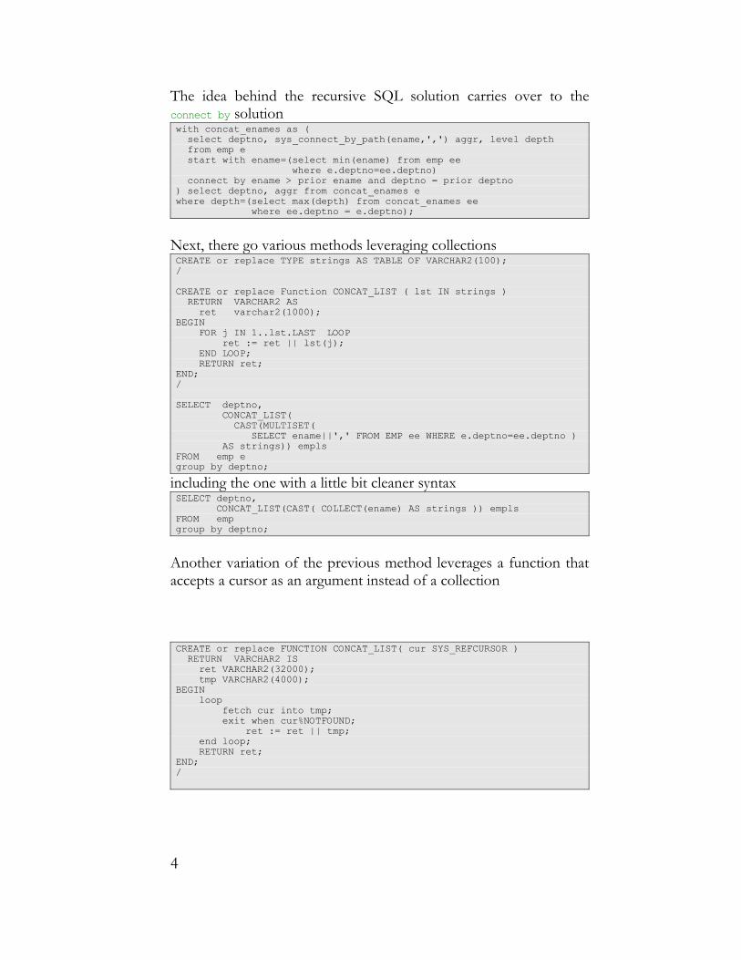
The idea behind the recursive SQL solution carries over to the connect by solutionwith concat_enames as ( select deptno, sys_connect_by_path(ename,',') aggr, level depth from emp e start with ename=(select min(ename) from emp ee where e.deptno=ee.deptno) connect by ename > prior ename and deptno = prior deptno) select deptno, aggr from concat_enames ewhere depth=(select max(depth) from concat_enames ee where ee.deptno = e.deptno);

Next, there go various methods leveraging collections CREATE or replace TYPE strings AS TABLE OF VARCHAR2(100);/ CREATE or replace Function CONCAT_LIST ( lst IN strings ) RETURN VARCHAR2 AS ret varchar2(1000); BEGIN FOR j IN 1..lst.LAST LOOP ret := ret || lst(j); END LOOP; RETURN ret; END;/ SELECT deptno, CONCAT_LIST( CAST(MULTISET( SELECT ename||',' FROM EMP ee WHERE e.deptno=ee.deptno ) AS strings)) empls FROM emp egroup by deptno;

including the one with a little bit cleaner syntaxSELECT deptno, CONCAT_LIST(CAST( COLLECT(ename) AS strings )) emplsFROM empgroup by deptno;

Another variation of the previous method leverages a function that accepts a cursor as an argument instead of a collection

CREATE or replace FUNCTION CONCAT_LIST( cur SYS_REFCURSOR ) RETURN VARCHAR2 IS ret VARCHAR2(32000); tmp VARCHAR2(4000);BEGIN loop fetch cur into tmp; exit when cur%NOTFOUND; ret := ret || tmp; end loop; RETURN ret;END;/

4

select distinct deptno, CONCAT_LIST(CURSOR( select ename ||',' from emp ee where e.deptno = ee.deptno ) employeesfrom emp e;

Admittedly, the function concatenating values in a collection adds a little bit of a procedural taste. Again, such general purpose function shouldn’t necessarily be exposed as a part of the solution at all. It is obvious that the CONCAT_LIST function should already be in the RDBMS library.

So far we counted half a dozen various aggregate string concatenation methods. Not all of them are created equal from performance perspective, of course. The most efficient solutions are the one with user-defined aggregation and the other one leveraging collect function. Don’t hastily dismiss the rest, however. If nothing else, the problem of writing a list aggregate is still a great job interview question. You can rate someone’s SQL skills (on the scale 0 to 6) by the number of different approaches that she can count.

Product Product is another aggregate function, which is not on the list of built-in SQL functions. Randomly browsing any mathematical book, however, reveals that the product symbol occurs much less frequently than summation. Therefore, it is unlikely to expect the product to grow outside a very narrow niche. Yet there are at least two meaningful applications.

FactorialIf the product aggregate function were available, it would make factorial calculation effortlessselect prod(num) from integers where num <=10 -- 10!

As always, a missing feature encourages people to become very inventive. From a math perspective, any multiplicative property can be translated into additive one, if we apply the logarithm function. Therefore, instead of multiplying numbers, we can add their

5

logarithms, and then exponentiate the result. The rewritten factorial queryselect exp(sum(ln(num))) from integers where num <=10

is still very succinct.

At this point most people realize that product via logarithms doesn’t work in all the cases. The ln SQL function throws an exception for negative numbers and zero. After recognizing this fact, however, we could fix the problem immediately with a case expression.

Writing a function calculating factorial is perhaps one of the most ubiquitous exercises in procedural programming. It is primarily used to demonstrate the recursion. It is very tempting, therefore, to try recursive SQL

with factorial (n, f) as ( values(1, 1) union all select n+1, f*(n+1) from factorial where n<10) select * from factorial

Numbers in SQLIf you feel uneasy about “fixing” an elegant exp(sum(ln(…))) expression with case analysis, it’s an indicator that you as a programmer reached a certain maturity level. Normally, there are no problems when generalizing clean and simple concepts in math. What exactly is broken?

The problem is that the logarithm is a multivalued function defined on complex numbers. For example, ln(-1) = i π (taken on principal branch). Then, e i π = -1 as expected!

6

Joe Celko suggested one more method - calculating factorial via Gamma function. A polynomial approximation with an error of less than 3*10-7 for 0 ≤ x ≤ 1 is:

Γ(x+1) = 1 - 0.577191652 x + 0.988205891 x2 - 0.897056937 x3 +

0.918206857 * x4 - 0.756704078 x5 + 0.482199394 x6 -

0.193527818 x7 + 0.035868343 x8

Unfortunately, the error grows significantly outside of the interval 0 ≤ x ≤ 1. For example,

Γ(6) = 59.589686421

Factorial alone could hardly be considered as a convincing case for the product aggregate function. While factorial is undoubtedly a cute mathematical object, in practice, it is never interesting to such an extent as to warrant a dedicated query. Most commonly factorial occurs as a part of more complex expression or query, and its value could be calculated on the spot with an unglamorous procedural method.

InterpolationInterpolation is more pragmatic justification for the product aggregate. Consider the following data

X Y 1 2 2 6 3 4 8 5 6 7 6

Can you guess the missing values?

When this SQL puzzle was posted on the Oracle OTN forum, somebody immediately reacted suggesting the lag and leading analytic functions as a basis for calculating intermediate values by averaging them. The problem is that the number of intermediate

7

values is not known in advance, so that my first impression was that the solution should require leveraging recursion or hierarchical SQL extension, at least. A breakthrough came from Gabe Romanescu, who posted the following analytic SQL solution:select X,Y ,case when Y is null then yLeft+(rn-1)*(yRight-yLeft)/cnt else Y end /*as*/ interp_Yfrom ( select X, Y ,count(*) over (partition by grpa) cnt ,row_number() over (partition by grpa order by X) rn ,avg(Y) over (partition by grpa) yLeft ,avg(Y) over (partition by grpd) yRight from ( select X, Y ,sum(case when Y is null then 0 else 1 end) over (order by X) grpa ,sum(case when Y is null then 0 else 1 end) over (order by X desc) grpd from data ));

As usual in case of complex queries with multiple levels of inner views, the best way to understand it is executing the query in small increments. The inner-most query select X, Y ,sum(case when Y is null then 0 else 1 end) over (order by X) grpa, ,sum(case when Y is null then 0 else 1 end) over (order by X desc) grpdfrom data;

X Y GRPA GRPD 1 2 1 4 2 6 2 3 3 2 2 4 8 3 2 5 3 1 6 3 1 7 6 4 1

introduces two new columns, with the sole purpose to group spans with missing values together.

The next step

8

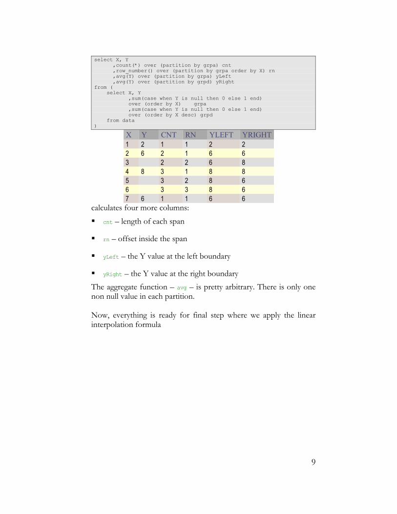
select X, Y ,count(*) over (partition by grpa) cnt ,row_number() over (partition by grpa order by X) rn ,avg(Y) over (partition by grpa) yLeft ,avg(Y) over (partition by grpd) yRightfrom ( select X, Y ,sum(case when Y is null then 0 else 1 end) over (order by X) grpa ,sum(case when Y is null then 0 else 1 end) over (order by X desc) grpd from data)

X Y CNT RN YLEFT YRIGHT 1 2 1 1 2 2 2 6 2 1 6 6 3 2 2 6 8 4 8 3 1 8 8 5 3 2 8 6 6 3 3 8 6 7 6 1 1 6 6

calculates four more columns: cnt – length of each span

rn – offset inside the span

yLeft – the Y value at the left boundary

yRight – the Y value at the right boundaryThe aggregate function – avg – is pretty arbitrary. There is only one non null value in each partition.

Now, everything is ready for final step where we apply the linear interpolation formula

9

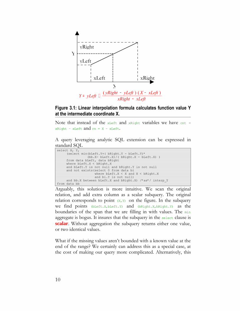
= Y + yLeft( ) − yRight yLeft ( ) − X xLeft

− xRight xLeft

Figure 3.1: Linear interpolation formula calculates function value Y at the intermediate coordinate X. Note that instead of the xLeft and xRight variables we have cnt = xRight – xLeft and rn = X - xLeft.

A query leveraging analytic SQL extension can be expressed in standard SQL select X, Y, (select min(bLeft.Y+( bRight.Y - bLeft.Y)* (bb.X- bLeft.X)/( bRight.X - bLeft.X) ) from data bLeft, data bRight where bLeft.X < bRight.X and bLeft.Y is not null and bRight.Y is not null and not exists(select 0 from data bi where bLeft.X < X and X < bRight.X and bi.Y is not null) and bb.X between bLeft.X and bRight.X) /*as*/ interp_Yfrom data bb

Arguably, this solution is more intuitive. We scan the original relation, and add extra column as a scalar subquery. The original relation corresponds to point (X,Y) on the figure. In the subquery we find points (bLeft.X,bLeft.Y) and (bRight.X,bRight.Y) as the boundaries of the span that we are filling in with values. The min aggregate is bogus. It insures that the subquery in the select clause is scalar. Without aggregation the subquery returns either one value, or two identical values.

What if the missing values aren’t bounded with a known value at the end of the range? We certainly can address this as a special case, at the cost of making our query more complicated. Alternatively, this

Y

X

yRight

yLeft

xRightxLeft

10

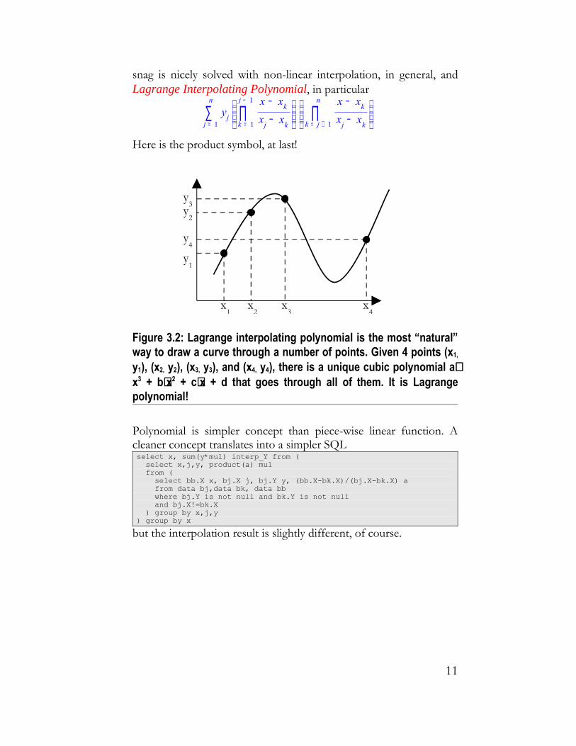
snag is nicely solved with non-linear interpolation, in general, and Lagrange Interpolating Polynomial, in particular

∑ = j 1

n

yj

∏

= k 1

− j 1 − x xk − xj xk

∏

= k + j 1

n − x xk − xj xk

Here is the product symbol, at last!

Figure 3.2: Lagrange interpolating polynomial is the most “natural” way to draw a curve through a number of points. Given 4 points (x1,

y1), (x2, y2), (x3, y3), and (x4, y4), there is a unique cubic polynomial a⋅x3 + b⋅x2 + c⋅x + d that goes through all of them. It is Lagrange polynomial!

Polynomial is simpler concept than piece-wise linear function. A cleaner concept translates into a simpler SQLselect x, sum(y*mul) interp_Y from ( select x,j,y, product(a) mul from ( select bb.X x, bj.X j, bj.Y y, (bb.X-bk.X)/(bj.X-bk.X) a from data bj,data bk, data bb where bj.Y is not null and bk.Y is not null and bj.X!=bk.X ) group by x,j,y) group by x

but the interpolation result is slightly different, of course.

y1

x1

x3

x4

y4

y3y2

x2

11

PivotPivot and Unpivot are two fundamental operators that exchange rows and columns. Pivot aggregates a set of rows into a single row with additional columns. Informally, given the Sales relation

Product Month Amount Shorts Jan 20 Shorts Feb 30 Shorts Mar 50 Jeans Jan 25 Jeans Feb 32 Jeans Mar 37 T-shirt Jan 10 T-shirt Feb 15

the pivot operator transforms it into a relation with fewer rows, and some column headings changed

Product Jan Feb Mar Shorts 20 30 50 Jeans 25 32 37 T-shirt 10 15

Unpivot is informally defined as a reverse operator, which alters this relation back into the original one.

A reader who is already familiar with the Conditional Summation idiom from chapter 1 would have no difficulty writing pivot query in standard SQLselect Product, sum(case when Month=’Jan’ then Amount else 0 end) Jan, sum(case when Month=’Feb’ then Amount else 0 end) Feb, sum(case when Month=’Mar’ then Amount else 0 end) Marfrom Salesgroup by Product

Why aggregation and grouping? Aggregation is a natural way to handle data collision, when several values map to the same location. For example, if we have two records of sales for the month of January, then it may be either an error in the input data, or the result of projection applied in the inner view. The original Sales relation might have the Month and Day columns, and projection simply discarded the day information. Then, summation is the right way to get the correct answer1.

1 It may be argued that it is the projection that should have taken care of aggregation, while pivot should simply throw in an exception in case of data collision

12

Unfortunately, the approach with the straightforward query above quickly shows its limitations. First, each column has a repetitive syntax which is impossible to factor in. More important, however, is our inability to accommodate a dynamic list of values. In this example, the (full) list of months is static, but change months to years, and we have a problem.

SQL Server 20052 introduced pivot operator as syntax extension for table expression in the from clauseselect * from (Sales pivot (sum(Amount) for Month in (’Jan’, ’Feb’, ’Mar’))

As soon as a new feature is introduced people start wondering if it can accommodate more complex cases. For example, can we do two aggregations at once? Given the Sales relation, can we output the sales total amounts together with sales counts like this Product JanCnt FebCnt MarCnt JanSum FebSum MarSum Shorts 1 1 1 20 30 50 Jeans 1 1 1 25 32 37 T-shirt 1 1 10 15

We had to change column names in order to accommodate extra columns and, if nothing else, the changed column names should hint the solution. The other idea, which should be immediately obvious from the way the table columns are arranged in the display, is that the result is a join between the two primitive pivot queries

Product JanCnt FebCnt MarCnt Shorts 1 1 1 Jeans 1 1 1 T-shirt 1 1

and Product JanSum FebSum MarSum Shorts 20 30 50 Jeans 25 32 37 T-shirt 10 15

Well, what about those fancy column names? There is nothing like JanCnt in the original data. Indeed there isn’t, but transforming the month column data into the new column with Cnt postfix can be 2 Conor Cunningham, Goetz Graefe, César A. Galindo-Legaria: PIVOT and UNPIVOT: Optimization and Execution Strategies in an RDBMS. VLDB 2004: 998-1009

13

done easily with string concatenation. Therefore, the answer to the problem isselect scount.*, ssum.* from (

select * from ( (select product, month || ‘Cnt’, amount from Sales) pivot (count(*) for Month in (’JanCnt’, ’FebCnt’, ’MarCnt’)

) scount, (select * from ( (select product, month || ‘Sum’, amount from Sales) pivot (sum(Amount) for Month in (’JanSum’, ’FebSum’, ’MarSum’)

) ssumwhere scount.product = ssum.product

When I posted this solution on SQL server programming forum, Adam Machanic objected that is very inefficient compared to the conditional summation versionselect Product, sum(case when Month=’Jan’ then 1 else 0 end) JanCnt, sum(case when Month=’Feb’ then 1 else 0 end) FebCnt, sum(case when Month=’Mar’ then 1 else 0 end) MarCnt, sum(case when Month=’Jan’ then Amount else 0 end) JanSum, sum(case when Month=’Feb’ then Amount else 0 end) FebSum, sum(case when Month=’Mar’ then Amount else 0 end) MarSumfrom Salesgroup by Product

The culprit is the pivot clause syntax. It would have been much more natural design if 1. the pivot operator were designed as shorthand for the

conditional summation query,

2. the pivot clause were allowed in a select list, rather than being a part of a table reference in the from clause.

The other popular request is pivot on multiple columns. Given the Sales relation extended with one extra column

Product Month Day Amount Shorts Jan 1 20 Shorts Jan 2 30 Shorts Jan 3 50 Jeans Feb 1 25 Jeans Feb 2 32 Jeans Feb 3 37

pivot it over the combination of Month and Day columns. This is much easier: all we need to do is concatenating the Month and the Day values and consider it as a pivot column:

14

select * from ( (select product, month || ‘_’ || day as Month_Day, amount from Sales) pivot (count(*) for Month_Day in (’Jan_1’, ’Jan_2’, ’Jan_3’, …)

)As this example demonstrates, the number of pivoted values easily becomes unwieldy, which warrants more syntactic enhancements.

Unpivot in standard SQL syntax isselect product, ’Jan’ as Month, Jan as Amount from PivotedSales union allselect product, ’Feb’ as Month, Feb as Amount from PivotedSales union allselect product, ’Mar’ as Month, Mar as Amount from PivotedSales

again repetitive and not dynamically extensible. In SQL Server 2005 syntax it becomesselect * from (PivotedSales unpivot (Amount for Month in (’Jan’, ’Feb’, ’Mar’))

Introduction of pivot and unpivot operators in SQL opens interesting possibilities for data modeling. It may reincarnate the outcast Entity-Attribute-Value (EAV) approach. EAV employs a single “property table” containing just three columns: propertyId, propertyName, and propertyValue. The EAV styled schema design has grave implication on how data in this form can (or rather cannot) be queried. Even the simplest aggregate with group by queries can’t be expressed without implicitly transforming the data into a more appropriate view. Indexing is also problematic. Regular tables routinely have composite indexes, while EAV table has to be self-joined or pivoted before we even get to a relation with more than one property value column. Pivot makes an EAV table look like a regular table.

Symmetric DifferenceSuppose there are two tables A and B with the same columns, and we would like to know if there is any difference in their contents.

15

The Symmetric Difference query( select * from A minus select * from B) union all ( select * from B minus select * from A)

provides a definitive answer.

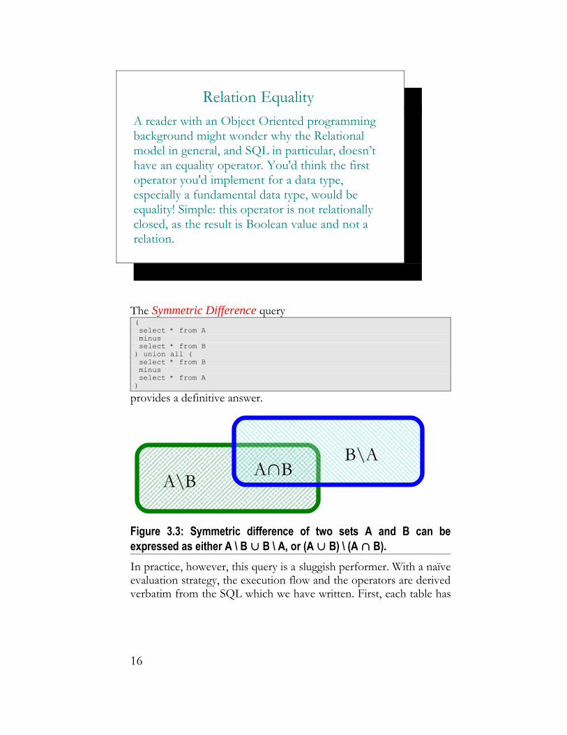
Figure 3.3: Symmetric difference of two sets A and B can be expressed as either A \ B ∪ B \ A, or (A ∪ B) \ (A ∩ B). In practice, however, this query is a sluggish performer. With a naïve evaluation strategy, the execution flow and the operators are derived verbatim from the SQL which we have written. First, each table has

Relation Equality A reader with an Object Oriented programming background might wonder why the Relational model in general, and SQL in particular, doesn’t have an equality operator. You'd think the first operator you'd implement for a data type, especially a fundamental data type, would be equality! Simple: this operator is not relationally closed, as the result is Boolean value and not a relation.

A\BB\A

A∩B

16

to be scanned twice. Then, four sort operators are applied in order to exclude duplicates. Next, the two set differences are computed, and, finally, the two results are combined together with the union operator.

RDBMS implementations today, however, have pretty impressive query transformation capabilities. In our case, set difference can already be internally rewritten as anti-join. If not then, perhaps, you might be able to influence the query optimizer to transform the query into the desired form. Otherwise, you have to explicitly rewrite it:select * from A where (col1,col2,…) not in (select col1,col2,… from B) union all select * from B where (col1,col2,…) not in (select col1,col2,… from A)

17

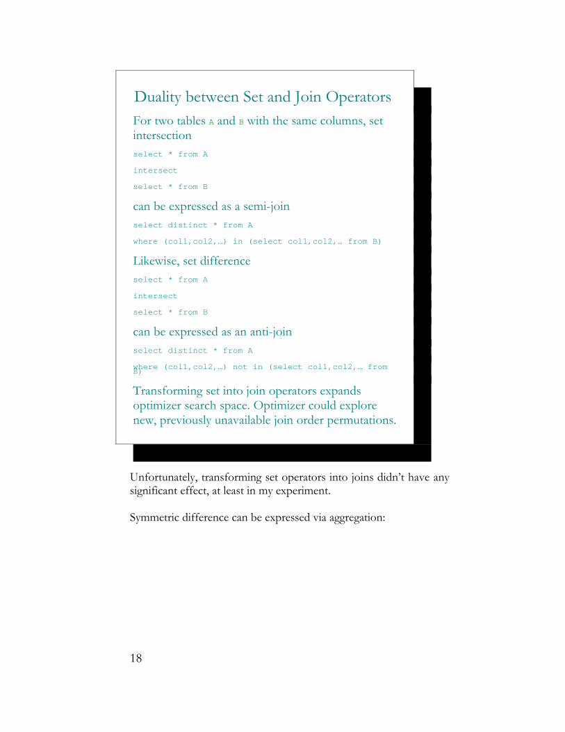
Unfortunately, transforming set operators into joins didn’t have any significant effect, at least in my experiment.

Symmetric difference can be expressed via aggregation:

Duality between Set and Join Operators For two tables A and B with the same columns, set intersection select * from A

intersect

select * from B

can be expressed as a semi-joinselect distinct * from A

where (col1,col2,…) in (select col1,col2,… from B)

Likewise, set differenceselect * from A

intersect

select * from B

can be expressed as an anti-joinselect distinct * from A

where (col1,col2,…) not in (select col1,col2,… from B)

Transforming set into join operators expands optimizer search space. Optimizer could explore new, previously unavailable join order permutations.

18

select * from ( select id, name, sum(case when src=1 then 1 else 0 end) cnt1, sum(case when src=2 then 1 else 0 end) cnt2 from ( select id, name, 1 src from A union all select id, name, 2 src from B ) group by id, name)where cnt1 <> cnt2

This appeared to be a rather elegant solution3 where each table has to be scanned once only, until we discover that it has about the same performance as the canonic symmetric difference query.

When comparing data in two tables there are actually two questions that one might want to ask:1. Is there any difference? The expected answer is Boolean.

2. What are the rows that one table contains, and the other doesn't.Question #1 can be answered faster than #2 with a hash value based technique.

The standard disclaimer of any hash-based technique is that it’s theoretically possible to get a wrong result. The rhetorical question, however, is how often did the reader experience a problem due to hash value collision? I never did. Would a user be willing to accept a (rather negligible) risk of getting an incorrect result for a significant performance boost?

In a hash-based method we associate each table with a single aggregated hash value: select sum( ora_hash(id||'|'||name, POWER(2,16)-1) )from A

There we concatenated all the row fields4, and then translated this string into a hash value. Alternatively, we could have calculated hash values for each field, and then apply some asymmetric function in order for the resulting hash value to be sensitive in respect to column permutations:

3 suggested by Marco Stefanetti in an exchange at the Ask Tom forum4 with a dedicated “|” separator, in order to guarantee uniqueness

19

select 1 * sum( ora_hash(id, POWER(2,16)-1) ) + 2 * sum( ora_hash(name, POWER(2,16)-1) )from A

Row hash values are added together with ordinary sum aggregate, but we could have written a modulo 216-1 user-defined aggregate hash_sum in the spirit of the CRC (Cyclic Redundancy Check) technique.

Hash value calculation time is proportional to the table size. This is noticeably better than the symmetric difference query, where the bottleneck was the sorting.

We can do even better, at the expense of introducing a materialized view. The hash value behaves like aggregate, and therefore, can be calculated incrementally. If a row is added into a table, then a new hash value is a function of the old hash value and the added row. Incremental evaluation means good performance, and the comparison between the two scalar hash values is done momentarily.

HistogramsThe concept of histograms originated in statistics. Admittedly, statistics never enjoyed the reputation of being the most exciting math subject. I never was able to overcome a (presumably unfair) impression that it is just a collection of ad-hoc methods. Yet a typical database table has huge volume of data, and histograms provide an opportunity to present it in compact human digestible report.

A histogram can be built on any (multi-)set of values. In the database world this set comes from a table column, so that values can be numerical, character, or other datatype. For our purposes it is convenient to order the values and then index them (fig. 3.3)

20

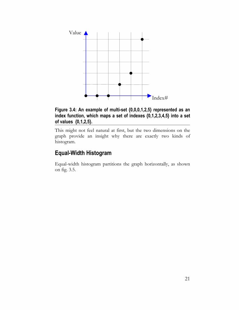
Figure 3.4: An example of multi-set {0,0,0,1,2,5} represented as an index function, which maps a set of indexes {0,1,2,3,4,5} into a set of values {0,1,2,5}. This might not feel natural at first, but the two dimensions on the graph provide an insight why there are exactly two kinds of histogram.

Equal-Width HistogramEqual-width histogram partitions the graph horizontally, as shown on fig. 3.5.

Index#

Value

21

Figure 3.5: Equal-width histogram partitioned the set {0,1,2,5} of values into sets {1,2}, {3}, and {5}. Evidently, there is something wrong here, either with the term equal- width histogram, or my unorthodox interpretation. First, the partitioning is vertical; second, why do buckets have to be of uniform size? Well, if we swap the coordinates in an attempt to make partitioning conform to its name, then it wouldn’t be a function any more. Also, partitioning doesn’t have to be uniform: we well study histograms with logarithmic partitioning later.

There is one special type of equal-width histogram – frequency histogram. It partitions the set of values in the finest possible way (fig 3.6).

Index#

Value

22

Figure 3.6: Frequency histogram is equal-width histogram with the finest possible partitioning of the value set.

Now that we have two kinds of objects -- the (indexed) values and buckets -- we associate them in a query. We could ask either what bucket a particular value falls in, or

what is the aggregate value in each bucket (we could be interested in more than one aggregate function)

In the first case, our query returns one extra attribute per each record in the input data. Given the input set of data

Index# Value 0 0 1 0 2 0 3 1 4 2 5 5

the expected output is

Index#

Value

23

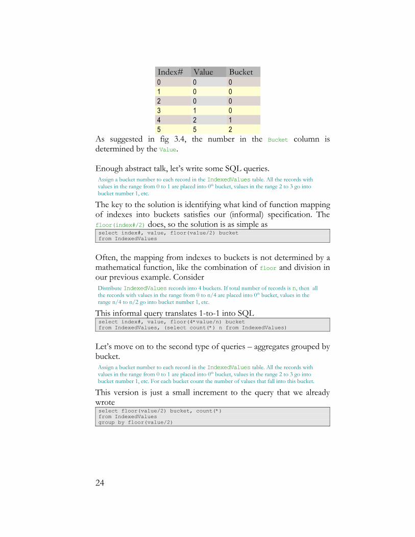
Index# Value Bucket 0 0 0 1 0 0 2 0 0 3 1 0 4 2 1 5 5 2

As suggested in fig 3.4, the number in the Bucket column is determined by the Value.

Enough abstract talk, let’s write some SQL queries. Assign a bucket number to each record in the IndexedValues table. All the records with values in the range from 0 to 1 are placed into 0th bucket, values in the range 2 to 3 go into bucket number 1, etc.

The key to the solution is identifying what kind of function mapping of indexes into buckets satisfies our (informal) specification. The floor(index#/2) does, so the solution is as simple as select index#, value, floor(value/2) bucketfrom IndexedValues

Often, the mapping from indexes to buckets is not determined by a mathematical function, like the combination of floor and division in our previous example. ConsiderDistribute IndexedValues records into 4 buckets. If total number of records is n, then all the records with values in the range from 0 to n/4 are placed into 0th bucket, values in the range n/4 to n/2 go into bucket number 1, etc.

This informal query translates 1-to-1 into SQL select index#, value, floor(4*value/n) bucketfrom IndexedValues, (select count(*) n from IndexedValues)

Let’s move on to the second type of queries – aggregates grouped by bucket.Assign a bucket number to each record in the IndexedValues table. All the records with values in the range from 0 to 1 are placed into 0th bucket, values in the range 2 to 3 go into bucket number 1, etc. For each bucket count the number of values that fall into this bucket.

This version is just a small increment to the query that we already wrote select floor(value/2) bucket, count(*)from IndexedValuesgroup by floor(value/2)

24

A simplified version of the previous query in verbose formAssign a bucket number to each record in the IndexedValues table. The record with value 0 is placed into 0th bucket, value 1 goes into bucket number 1, etc. For each bucket count the number of values that fall into this bucket.

defines a frequency histogram. It is formally expressed as celebrated group by queryselect value bucket, count(*)from IndexedValuesgroup by value

Equal-Height HistogramEqual-height histogram partitions the graph vertically, as shown on fig. 3.7.

Figure 3.7: Equal-height histogram partitioned the set {0,1,2,3,4,5} of indexes into sets {0,1}, {2,3}, and {4,5}. As a reader might have guessed already, the development in the rest of the section would mimic equal-width case with the value and index# roles reversed. There is some asymmetry, though. Unlike the equal-width case where partitioning values with the finest granularity led to the introduction of the frequency histogram, there is nothing interesting about partitioning indexes to the extreme. Each bucket corresponds one-to-one to the index, so that we don’t need the concept of a bucket anymore.

Index#

Value

25

Let’s proceed straight to queries. They require little thought other than formal substitution of value by index#.Assign a bucket number to each record in the IndexedValues table. All the records with indexes in the range from 0 to 1 are placed into 0th bucket, indexes in the range 2 to 3 go into bucket number 1, etc. select index#, value, floor(index#/2) bucketfrom IndexedValues

There is one subtlety for aggregate query. The record count within each bucket is not interesting anymore, as in our example we know it’s trivially 2. We might ask other aggregate functions, though.Assign a bucket number to each record in the IndexedValues table. All the records with indexes in the range from 0 to 1 are placed into 0th bucket, indexes in the range from 2 to 3 go into bucket number 1, etc. For each bucket find the maximum and minimum value.select floor(index#/2) bucket, min(value), max(value)from IndexedValuesgroup by floor(index#/2)

Logarithmic BucketsBird’s-eye view onto big tables is essential for data analysis, with aggregation and grouping being the tools of the trade. Standard, equality-based grouping, however, fails to accommodate continuous distributions of data. Consider a TaxReturns table, for example. Would simple grouping by GrossIncome achieve anything? We’ll undoubtedly spot many individuals with identical incomes, but the big picture would escape us because of the sheer report size. Normally, we would like to know the distribution of incomes by ranges of values. By choosing the ranges carefully we might hope to produce a much more compact report.

There are two elementary methods for choosing ranges. With a linear scale we position the next range boundary point by a uniform offset. With a logarithmic scale the offset is increased exponentially. In our tax returns example a familiar linear scale of ranges is 0 – 10K, 10K – 20K, 20K – 30K, …, while the logarithmic scale is …, 1K –10K, 10K – 100K, 100K – 1000K, … Although a linear scale is conceptually simpler, a logarithmic scale is more natural. It appears that a linear scale has more precision where most tax returns are located, but this is solely by virtue of the magic number 10K that we have chosen as an increment. Had we settled upon different figure, say 100K, then the precision would have been lost.

26

In a capitalist system income is not bounded. There are numerous individuals whose income goes far beyond the ranges where the most people exist. As of 2005 there were 222 billionaires in the US. They all don’t fit in the same tiny 10K bucket of incomes, of course. Most likely each would be positioned in its unique range, so that we have to have 222 10K ranges in order to accommodate only them!

From logarithmic perspective, however, a $1B person is “only” 5 ranges away from a $10K party. The logarithmic scale report is compact no matter how skewed the distribution is. Changing the factor of 10 into, say, 2 would increase the report size by a factor of log2(10)≈3, which could still qualify as a compact report. In a sense, the choice of factor in logarithmic scale is irrelevant.

Let’s implement logarithmic scale grouping of incomes in SQL. All that we need is power, log, and floor functions:

Logarithmic Scale in ProgrammingI often hear a fellow programmer suggesting “Let’s allocate 2K of memory”. Why 2K? Well, this size sounds about right for this particular data structure. Fine, if this structure is static, but what about dynamic ones, like any collection type? Allocating 2K every time when we need to grow the structure may be fine by today’s standard, but this magic number 2K would look ridiculous a decade later.

Logarithmic scale, however, provides an immortal solution. “Last time I allocated X bytes of memory, let’s allocate twice of that this time”. In short, there is no room for linear solutions in the world abiding by Moore’s law.

27

select power(10,floor(log(10,GrossIncome))), count(1) from TaxReturnsgroup by floor(log(10,GrossIncome));

It is the floor(log(10,GrossIncome)) function that maps logarithmically spaced range boundaries into a distinct numbers. We group by this expression, although for the purpose of the readability of the result set it is convenient to transform the column expression within the select list into conventional salary units by exponentiating it.

Skyline QuerySuppose you are shopping for a new car, and are specifically looking for a big car with decent gas mileage. Unfortunately, we are trying to satisfy the two conflicting goals. If we are querying the Cars relation in the database, then we certainly can ignore all models that are worse than others by both criteria. The remaining set of cars is called the Skyline.

Figure 3.1 shows the Skyline of all cars in a sample set of 3 models. The vertical axis is seating capacity while the horizontal axis is the gas mileage. The vehicles are positioned in such a way that their locations match their respective profiles. The Hummer is taller than the Ferrari F1 racing car, which reflects the difference in their seating accommodations: 4 vs. 1. The Ferrari protrudes to the right of the Hummer, because it has superior gas mileage.

28

Figure 3.8: Skyline of Car Profiles. Ferrari F1 loses to Roadster by both gas mileage and seating capacity criteria.

The Skyline is visualized as a contour of solid lines. The Ferrari outline is lost beneath the Roadster.

More formally the Skyline is defined as those points which are not dominated by any other point. A point dominates the other point if it is as good or better in all the dimensions. In our example Roadster with mileage=20 and seating=2 dominates Ferrari F1 with mileage=10 and seating=1. This condition can certainly be expressed in SQL. In our example, the Skyline query isselect * from Cars cwhere not exists ( select * from Cars cc where cc.seats >= c.seats and cc.mileage > c.mileage or cc.seats > c.seats and cc.mileage >= c.mileage);

Despite the apparent simplicity of this query, you wouldn’t be pleased with this query performance. Even if we index the seats and mileage columns, this wouldn’t help much as only half of the records on average meet each individual inequality condition. Certainly, there aren’t many records that satisfy the combined predicate, but we can’t

Mileage

Seats

5 10 20

421

29

leverage an index to match it. Bitmapped indexes, which excel with Boolean expressions similar to what we have, demand a constant on one side of the inequality predicate.

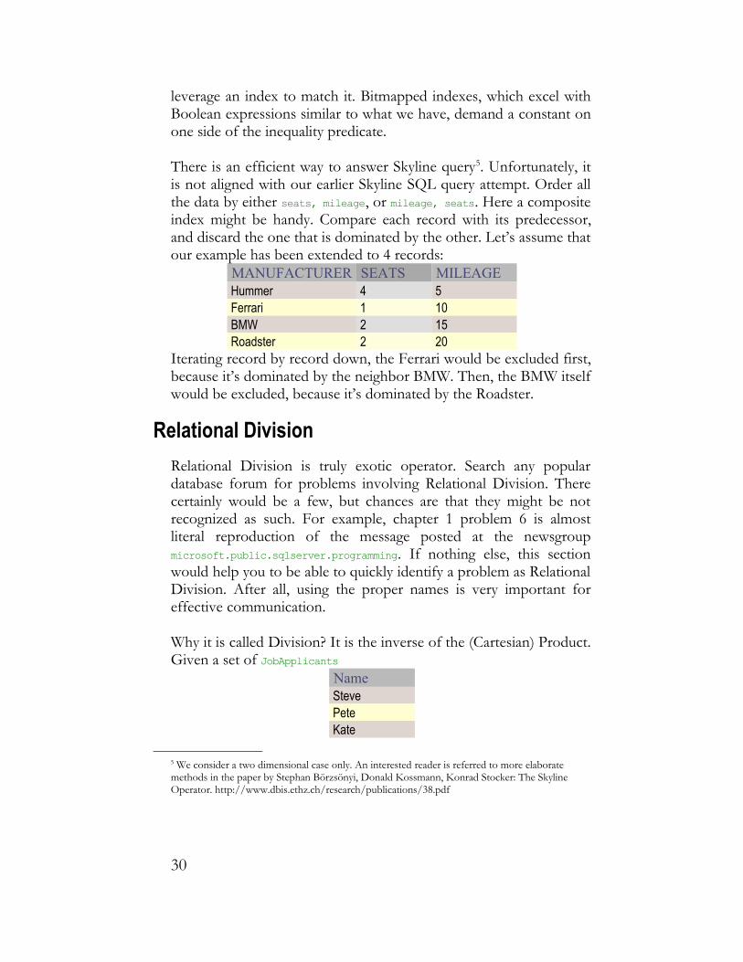
There is an efficient way to answer Skyline query5. Unfortunately, it is not aligned with our earlier Skyline SQL query attempt. Order all the data by either seats, mileage, or mileage, seats. Here a composite index might be handy. Compare each record with its predecessor, and discard the one that is dominated by the other. Let’s assume that our example has been extended to 4 records:

MANUFACTURER SEATS MILEAGE Hummer 4 5 Ferrari 1 10 BMW 2 15 Roadster 2 20

Iterating record by record down, the Ferrari would be excluded first, because it’s dominated by the neighbor BMW. Then, the BMW itself would be excluded, because it’s dominated by the Roadster.

Relational DivisionRelational Division is truly exotic operator. Search any popular database forum for problems involving Relational Division. There certainly would be a few, but chances are that they might be not recognized as such. For example, chapter 1 problem 6 is almost literal reproduction of the message posted at the newsgroup microsoft.public.sqlserver.programming. If nothing else, this section would help you to be able to quickly identify a problem as Relational Division. After all, using the proper names is very important for effective communication.

Why it is called Division? It is the inverse of the (Cartesian) Product. Given a set of JobApplicants

Name Steve Pete Kate

5 We consider a two dimensional case only. An interested reader is referred to more elaborate methods in the paper by Stephan Börzsönyi, Donald Kossmann, Konrad Stocker: The Skyline Operator. http://www.dbis.ethz.ch/research/publications/38.pdf

30

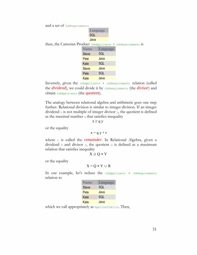
and a set of JobRequirements Language SQL Java

then, the Cartesian Product JobApplicants × JobRequirements is Name Language Steve SQL Pete Java Kate SQL Steve Java Pete SQL Kate Java

Inversely, given the JobApplicants × JobRequirements relation (called the dividend), we could divide it by JobRequirements (the divisor) and obtain JobApplicants (the quotient).

The analogy between relational algebra and arithmetic goes one step further. Relational division is similar to integer division. If an integer dividend x is not multiple of integer divisor y, the quotient is defined as the maximal number q that satisfies inequality

x ≥ q y

or the equalityx = q y + r

where r is called the remainder. In Relational Algebra, given a dividend X and divisor Y, the quotient Q is defined as a maximum relation that satisfies inequality

X ⊇ Q × Y

or the equality X = Q × Y ∪ R

In our example, let’s reduce the JobApplicants × JobRequirements relation to

Name Language Steve SQL Pete Java Kate SQL Kate Java

which we call appropriately as ApplicantSkills. Then,

31

ApplicantSkills = QualifiedApplicants × JobRequirements ∪

UnqualifiedSkillswhere the quotient QualifiedApplicants is

Name Kate

and the remainder UnqualifiedSkills is Name Language Steve SQL Pete Java

Informally, division identifies attribute values of the dividend that are associated with every member of the divisor:Find job applicants who meet all job requirements.

Relational Division is not a fundamental operator. It can be expressed in terms of projection, Cartesian product, and set difference. The critical observation is that multiplying the projection6

πName(ApplicantSkills) and JobRequirements results in the familiar Cartesian Product

Name Language Steve SQL Pete Java Kate SQL Steve Java Pete SQL Kate Java

Subtract ApplicantSkills, then project the result to get the Names of all the applicants who are not qualified. Finally, find all the applicants who are qualified as a complement to the set of all applicants. Formally

QualifiedApplicants = πName(ApplicantSkills)-- πName( πName(ApplicantSkills)×JobRequirements – ApplicantSkills )

Translating it into SQL is quite straightforward, although the resulting query gets quite unwieldyselect distinct Name from ApplicantSkillsminusselect Name from ( select Name, Language from ( select Name from ApplicantSkills

6 This is the very first time I used the projection symbol. The Relational Algebra projection operator πName(ApplicantSkills) is the succinct equivalent to SQL query select distinct Name from ApplicantSkills

32

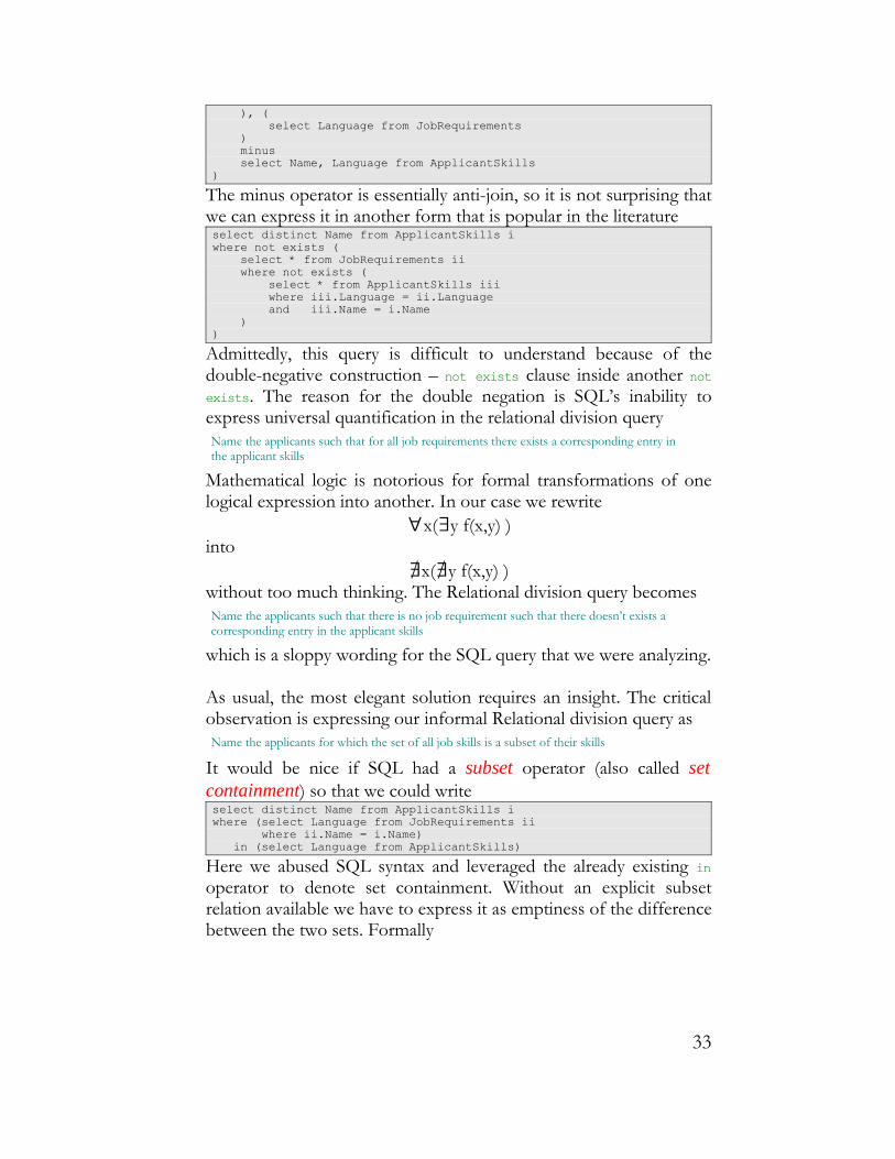
), ( select Language from JobRequirements ) minus select Name, Language from ApplicantSkills)

The minus operator is essentially anti-join, so it is not surprising that we can express it in another form that is popular in the literatureselect distinct Name from ApplicantSkills iwhere not exists ( select * from JobRequirements ii where not exists ( select * from ApplicantSkills iii where iii.Language = ii.Language and iii.Name = i.Name ))

Admittedly, this query is difficult to understand because of the double-negative construction – not exists clause inside another not exists. The reason for the double negation is SQL’s inability to express universal quantification in the relational division query Name the applicants such that for all job requirements there exists a corresponding entry in the applicant skills

Mathematical logic is notorious for formal transformations of one logical expression into another. In our case we rewrite

∀x(∃y f(x,y) )into

∄x(∄y f(x,y) )without too much thinking. The Relational division query becomesName the applicants such that there is no job requirement such that there doesn’t exists a corresponding entry in the applicant skills

which is a sloppy wording for the SQL query that we were analyzing.

As usual, the most elegant solution requires an insight. The critical observation is expressing our informal Relational division query asName the applicants for which the set of all job skills is a subset of their skills

It would be nice if SQL had a subset operator (also called set containment) so that we could writeselect distinct Name from ApplicantSkills iwhere (select Language from JobRequirements ii where ii.Name = i.Name) in (select Language from ApplicantSkills)

Here we abused SQL syntax and leveraged the already existing in operator to denote set containment. Without an explicit subset relation available we have to express it as emptiness of the difference between the two sets. Formally

33

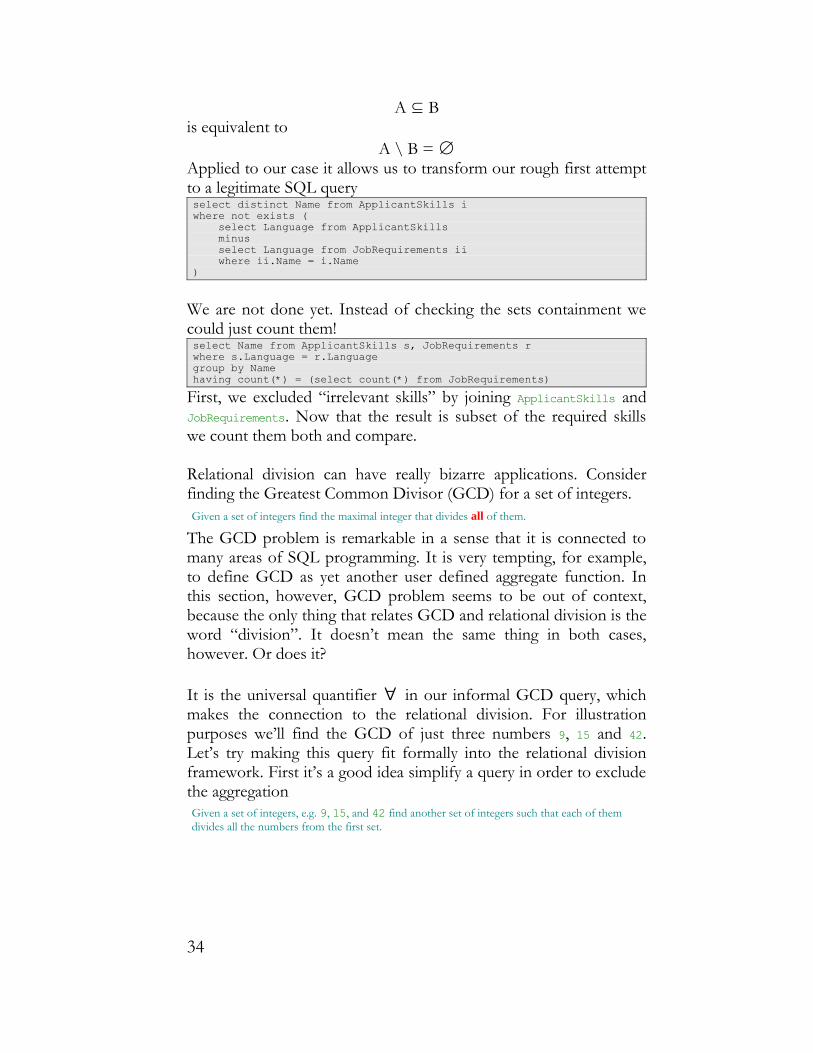
A ⊆ Bis equivalent to

A \ B = ∅Applied to our case it allows us to transform our rough first attempt to a legitimate SQL query select distinct Name from ApplicantSkills iwhere not exists ( select Language from ApplicantSkills minus select Language from JobRequirements ii where ii.Name = i.Name)

We are not done yet. Instead of checking the sets containment we could just count them! select Name from ApplicantSkills s, JobRequirements rwhere s.Language = r.Languagegroup by Namehaving count(*) = (select count(*) from JobRequirements)

First, we excluded “irrelevant skills” by joining ApplicantSkills and JobRequirements. Now that the result is subset of the required skills we count them both and compare.

Relational division can have really bizarre applications. Consider finding the Greatest Common Divisor (GCD) for a set of integers. Given a set of integers find the maximal integer that divides all of them.

The GCD problem is remarkable in a sense that it is connected to many areas of SQL programming. It is very tempting, for example, to define GCD as yet another user defined aggregate function. In this section, however, GCD problem seems to be out of context, because the only thing that relates GCD and relational division is the word “division”. It doesn’t mean the same thing in both cases, however. Or does it?

It is the universal quantifier ∀ in our informal GCD query, which makes the connection to the relational division. For illustration purposes we’ll find the GCD of just three numbers 9, 15 and 42. Let’s try making this query fit formally into the relational division framework. First it’s a good idea simplify a query in order to exclude the aggregationGiven a set of integers, e.g. 9, 15, and 42 find another set of integers such that each of them divides all the numbers from the first set.

34

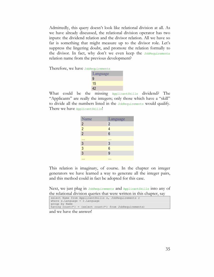
Admittedly, this query doesn’t look like relational division at all. As we have already discussed, the relational division operator has two inputs: the dividend relation and the divisor relation. All we have so far is something that might measure up to the divisor role. Let’s suppress the lingering doubt, and promote the relation formally to the divisor. In fact, why don’t we even keep the JobRequirements relation name from the previous development?

Therefore, we have JobRequirements Language 9 15 42

What could be the missing ApplicantSkills dividend? The “Applicants” are really the integers; only those which have a “skill” to divide all the numbers listed in the JobRequirements would qualify. There we have ApplicantSkills!

Name Language 2 2 2 4 2 6 … … 3 3 3 6 3 9 … …

This relation is imaginary, of course. In the chapter on integer generators we have learned a way to generate all the integer pairs, and this method could in fact be adopted for this case.

Next, we just plug in JobRequirements and ApplicantSkills into any of the relational division queries that were written in this chapter, sayselect Name from ApplicantSkills s, JobRequirements rwhere s.Language = r.Languagegroup by Namehaving count(*) = (select count(*) from JobRequirements)

and we have the answer!

35

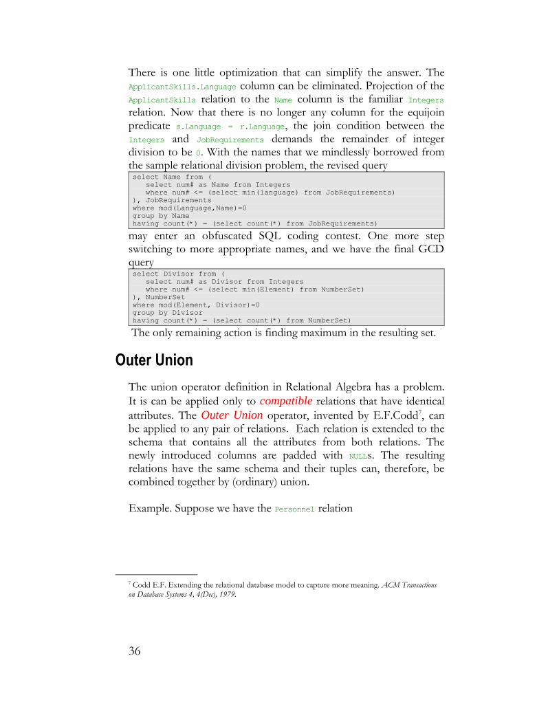
There is one little optimization that can simplify the answer. The ApplicantSkills.Language column can be eliminated. Projection of the ApplicantSkills relation to the Name column is the familiar Integers relation. Now that there is no longer any column for the equijoin predicate s.Language = r.Language, the join condition between the Integers and JobRequirements demands the remainder of integer division to be 0. With the names that we mindlessly borrowed from the sample relational division problem, the revised queryselect Name from ( select num# as Name from Integers where num# <= (select min(language) from JobRequirements)), JobRequirements where mod(Language,Name)=0group by Namehaving count(*) = (select count(*) from JobRequirements)

may enter an obfuscated SQL coding contest. One more step switching to more appropriate names, and we have the final GCD query select Divisor from ( select num# as Divisor from Integers where num# <= (select min(Element) from NumberSet)), NumberSet where mod(Element, Divisor)=0group by Divisorhaving count(*) = (select count(*) from NumberSet)

The only remaining action is finding maximum in the resulting set.

Outer UnionThe union operator definition in Relational Algebra has a problem. It is can be applied only to compatible relations that have identical attributes. The Outer Union operator, invented by E.F.Codd7, can be applied to any pair of relations. Each relation is extended to the schema that contains all the attributes from both relations. The newly introduced columns are padded with NULLs. The resulting relations have the same schema and their tuples can, therefore, be combined together by (ordinary) union.

Example. Suppose we have the Personnel relation

7 Codd E.F. Extending the relational database model to capture more meaning. ACM Transactions on Database Systems 4, 4(Dec), 1979.

36

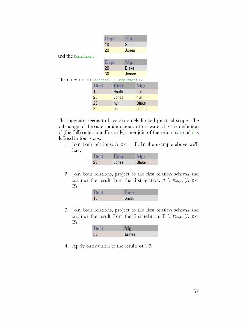
Dept Emp 10 Smith 20 Jones

and the Department Dept Mgr 20 Blake 30 James

The outer union Personnel ⊎ Department is Dept Emp Mgr 10 Smith null 20 Jones null 20 null Blake 30 null James

This operator seems to have extremely limited practical scope. The only usage of the outer union operator I’m aware of is the definition of (the full) outer join. Formally, outer join of the relations A and B is defined in four steps:

1. Join both relations: A B. In the example above we’ll have

Dept Emp Mgr 20 Jones Blake

2. Join both relations, project to the first relation schema and subtract the result from the first relation: A \ πsch(A) (A B)

Dept Emp 10 Smith

3. Join both relations, project to the first relation schema and subtract the result from the first relation: B \ πsch(B) (A B)

Dept Mgr 30 James

4. Apply outer union to the results of 1-3.

37

5. Dept Emp Mgr 10 Smith null 20 Jones Blake 30 null James

What we have just discussed are actually the relational algebra versions of the outer union and outer join operations. Perhaps they should be properly named natural outer union and natural outer join. In SQL the two relations are always considered to have disjoint sets of attributes. In our example, the outer union produces

Personnel.Dept Department.Dept Emp Mgr 10 null Smith null 20 null Jones null null 20 null Blake null 30 null James

and outer join Personnel.Dept Department.Dept Emp Mgr 10 null Smith null 20 20 Jones Blake null 30 null James

The formula connecting them is still valid, though.

Summary

Extensible RDBMS supports user defined-aggregate functions. They could be either programmed as user-defined functions, or implemented by leveraging object-relational features.

Rows could be transformed into columns via pivot operator.

Symmetric Difference is the canonic way to compare two tables.

Logarithmic histograms provide comprehensive summary of the data, which is immune to scaling.

Relational division is used to express queries with the universal quantifier ∀ (i.e. “for all”).

Outer union can be applied to incompatible relations.

38

Exercises1. Design a method to influence the order of summands of the

LIST aggregate function. 2. Check the execution plan of the symmetric difference query

in your database environment. Does it use set or join operations? If the former, persuade the optimizer to transform set into join. Which join method do you see in the plan? Can you influence the nested loops anti-join8? Is there noticeable difference in performance between all the alternative execution plans?

3. Binomial coefficient x choose y is defined by the formula

=

xy

!x!y !( ) − x y

where n! is n-factorial. Implement it as SQL query.4. Write down the following query

select distinct Name from ApplicantSkillsinformally in English. Try to make it sound as close as possible to the Relational Division. What is the difference?

5. A tuple t1 subsumes another tuple t2, if t2 has more null values than t1, and they coincide in all non- null attributes. The minimum union of two relations is defined as an outer union with subsequent removal of all the tuples subsumed by the others. Suppose we have two relations R1 and R2 with all the tuples subsumed by the others removed as well. Prove that the outer join between R1 and R2 is the minimum union of R1, R2 and R1 R2.

6. Check if your RDBMS of choice supplies some ad-hoc functions, which could be plugged into histogram queries. Oracle users are referred to ntile and width_bucket.

7. Write SQL queries that produce natural outer union and natural outer join.

8. Relational division is the prototypical example of a set join. Set joins relate database elements on the basis of sets of values, rather than single values as in a standard natural join. Thus, the division R(x, y)/S(y) returns a set of single value tuples

8 Nested Loops have acceptable performance with indexed access to the inner relation. The index role is somewhat similar to that of hash table in case of the Hash Join.

39

{ (x) | {y | R(x, y)} ⊇ {y | S(y)} }

More generally, one has the set-containment join of R(x, y) and S(y, z), which returns a set of pairs

{ (x, z) | {y | R(x, y)} ⊇ {y | S(y, z)} }

In the job applicants example we can extend the JobRequirements table with the column JobName. Then, listing all the applicants together with jobs they are qualified for is a set containment query. Write it in SQL.

40