spss-applications (data analysis) - luchsinger mathematics ag
TRANSCRIPT
Slide 1
CORTEX fellows training course, University of Zurich, October 2006
SPSS-Applications (Data Analysis)
Dr. Jürg Schwarz, [email protected]
Program 19. October 2006: Morning Lessons (0900-1200)
SPSS Basics
- Working with SPSS => parts of "The Basics… "
- Special issues: Use of Syntax Editor, Select Cases & Split File
Data Analysis with SPSS
- SPSS-Methods (Description, Testing, Modeling)
- Some notes about… (only "Type of Scales")
Slide 2
CORTEX fellows training course, University of Zurich, October 2006
Program 19. October 2006: Afternoon Lessons (1330-1630)
Extended Example: Multiple Regression
- Key steps
- Multiple Regression with SPSS
Exercise
- Multiple Regression
Slide 3
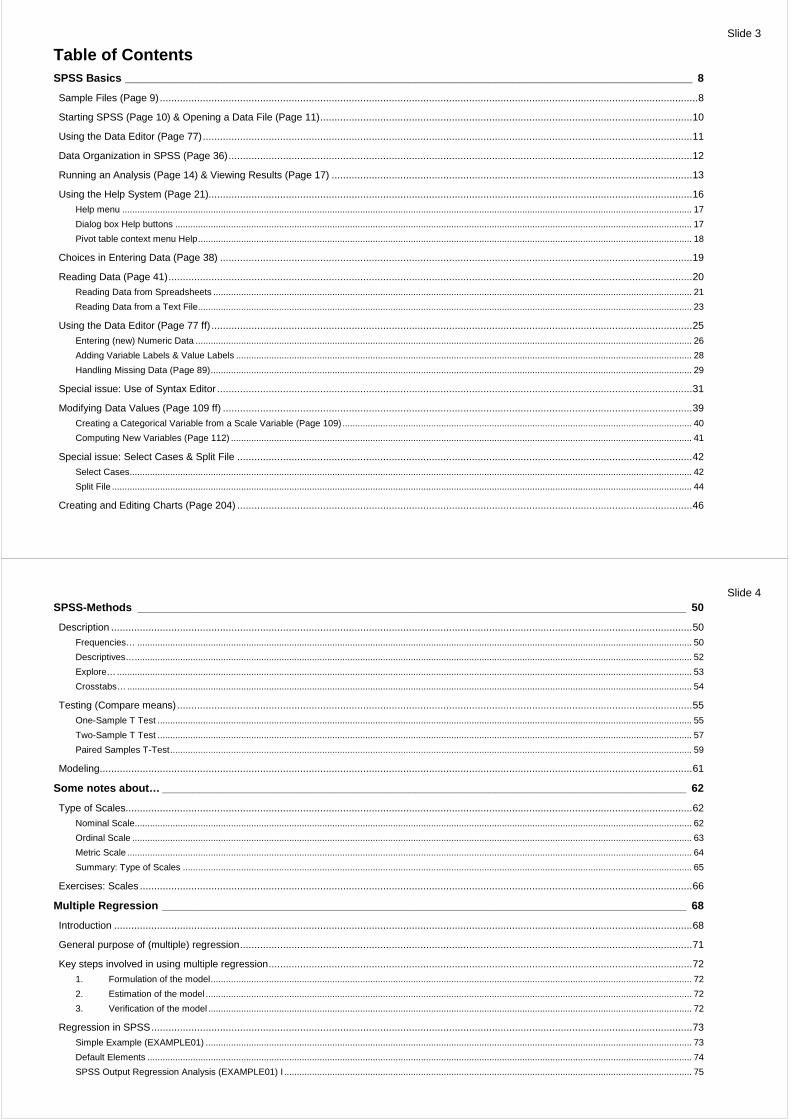
Table of Contents SPSS Basics ________________________________________ ____________________________________________________ 8
Sample Files (Page 9) ............................................................................................................................................................................................8
Starting SPSS (Page 10) & Opening a Data File (Page 11)..................................................................................................................................10
Using the Data Editor (Page 77)...........................................................................................................................................................................11
Data Organization in SPSS (Page 36)..................................................................................................................................................................12
Running an Analysis (Page 14) & Viewing Results (Page 17) ..............................................................................................................................13
Using the Help System (Page 21).........................................................................................................................................................................16 Help menu ................................................................................................................................................................................................................................. 17 Dialog box Help buttons ............................................................................................................................................................................................................ 17 Pivot table context menu Help................................................................................................................................................................................................... 18
Choices in Entering Data (Page 38) .....................................................................................................................................................................19
Reading Data (Page 41).......................................................................................................................................................................................20 Reading Data from Spreadsheets ............................................................................................................................................................................................. 21 Reading Data from a Text File................................................................................................................................................................................................... 23
Using the Data Editor (Page 77 ff) ........................................................................................................................................................................25 Entering (new) Numeric Data .................................................................................................................................................................................................... 26 Adding Variable Labels & Value Labels .................................................................................................................................................................................... 28 Handling Missing Data (Page 89).............................................................................................................................................................................................. 29
Special issue: Use of Syntax Editor ......................................................................................................................................................................31
Modifying Data Values (Page 109 ff) ....................................................................................................................................................................39 Creating a Categorical Variable from a Scale Variable (Page 109) .......................................................................................................................................... 40 Computing New Variables (Page 112) ...................................................................................................................................................................................... 41
Special issue: Select Cases & Split File ...............................................................................................................................................................42 Select Cases.............................................................................................................................................................................................................................. 42 Split File ..................................................................................................................................................................................................................................... 44
Creating and Editing Charts (Page 204) ...............................................................................................................................................................46
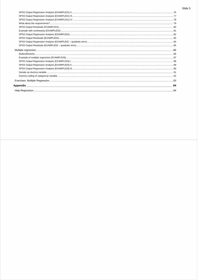
Slide 4 SPSS-Methods _______________________________________ __________________________________________________ 50
Description ...........................................................................................................................................................................................................50 Frequencies… ........................................................................................................................................................................................................................... 50 Descriptives…............................................................................................................................................................................................................................ 52 Explore…................................................................................................................................................................................................................................... 53 Crosstabs…............................................................................................................................................................................................................................... 54
Testing (Compare means)....................................................................................................................................................................................55 One-Sample T Test ................................................................................................................................................................................................................... 55 Two-Sample T Test ................................................................................................................................................................................................................... 57 Paired Samples T-Test.............................................................................................................................................................................................................. 59
Modeling...............................................................................................................................................................................................................61
Some notes about… __________________________________ ___________________________________________________ 62
Type of Scales......................................................................................................................................................................................................62 Nominal Scale............................................................................................................................................................................................................................ 62 Ordinal Scale ............................................................................................................................................................................................................................. 63 Metric Scale ............................................................................................................................................................................................................................... 64 Summary: Type of Scales ......................................................................................................................................................................................................... 65
Exercises: Scales .................................................................................................................................................................................................66
Multiple Regression ________________________________ _____________________________________________________ 68
Introduction ..........................................................................................................................................................................................................68
General purpose of (multiple) regression..............................................................................................................................................................71
Key steps involved in using multiple regression....................................................................................................................................................72 1. Formulation of the model.............................................................................................................................................................................................. 72 2. Estimation of the model ................................................................................................................................................................................................ 72 3. Verification of the model ............................................................................................................................................................................................... 72
Regression in SPSS.............................................................................................................................................................................................73 Simple Example (EXAMPLE01) ................................................................................................................................................................................................ 73 Default Elements ....................................................................................................................................................................................................................... 74 SPSS Output Regression Analysis (EXAMPLE01) I ................................................................................................................................................................. 75
Slide 5 SPSS Output Regression Analysis (EXAMPLE01) II ................................................................................................................................................................ 76 SPSS Output Regression Analysis (EXAMPLE01) III ............................................................................................................................................................... 77 SPSS Output Regression Analysis (EXAMPLE01) IV .............................................................................................................................................................. 78 What about the requirements? .................................................................................................................................................................................................. 79 SPSS Output Residuals (EXAMPLE01).................................................................................................................................................................................... 80 Example with nonlinearity (EXAMPLE02) ................................................................................................................................................................................. 81 SPSS Output Regression Analysis (EXAMPLE02) ................................................................................................................................................................... 82 SPSS Output Residuals (EXAMPLE02).................................................................................................................................................................................... 83 SPSS Output Regression Analysis (EXAMPLE02 – quadratic term)........................................................................................................................................ 84 SPSS Output Residuals (EXAMPLE02 – quadratic term)......................................................................................................................................................... 85
Multiple regression ...............................................................................................................................................................................................86 Multicollinearity .......................................................................................................................................................................................................................... 86 Example of multiple regression (EXAMPLE03)......................................................................................................................................................................... 87 SPSS Output Regression Analysis (EXAMPLE03) I ................................................................................................................................................................. 88 SPSS Output Regression Analysis (EXAMPLE03) II ................................................................................................................................................................ 89 SPSS Output Regression Analysis (EXAMPLE03) III ............................................................................................................................................................... 90 Gender as dummy variable ....................................................................................................................................................................................................... 91 Dummy coding of categorical variable ...................................................................................................................................................................................... 92
Exercises: Multiple Regression.............................................................................................................................................................................93
Appendix ___________________________________________ ___________________________________________________ 94
Help Regression...................................................................................................................................................................................................94
Slide 7
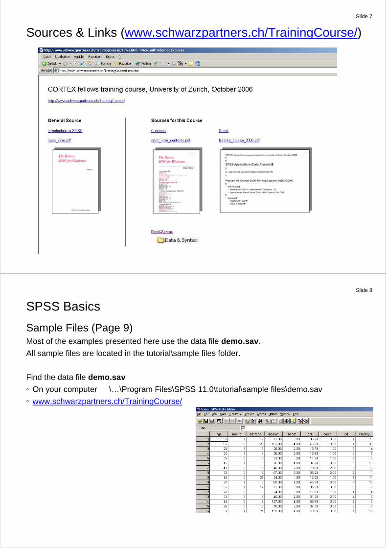
Sources & Links (www.schwarzpartners.ch/TrainingCourse/)
Slide 8
SPSS Basics
Sample Files (Page 9) Most of the examples presented here use the data file demo.sav .
All sample files are located in the tutorial\sample files folder.
Find the data file demo.sav
On your computer \…\Program Files\SPSS 11.0\tutorial\sample files\demo.sav
www.schwarzpartners.ch/TrainingCourse/
Slide 9
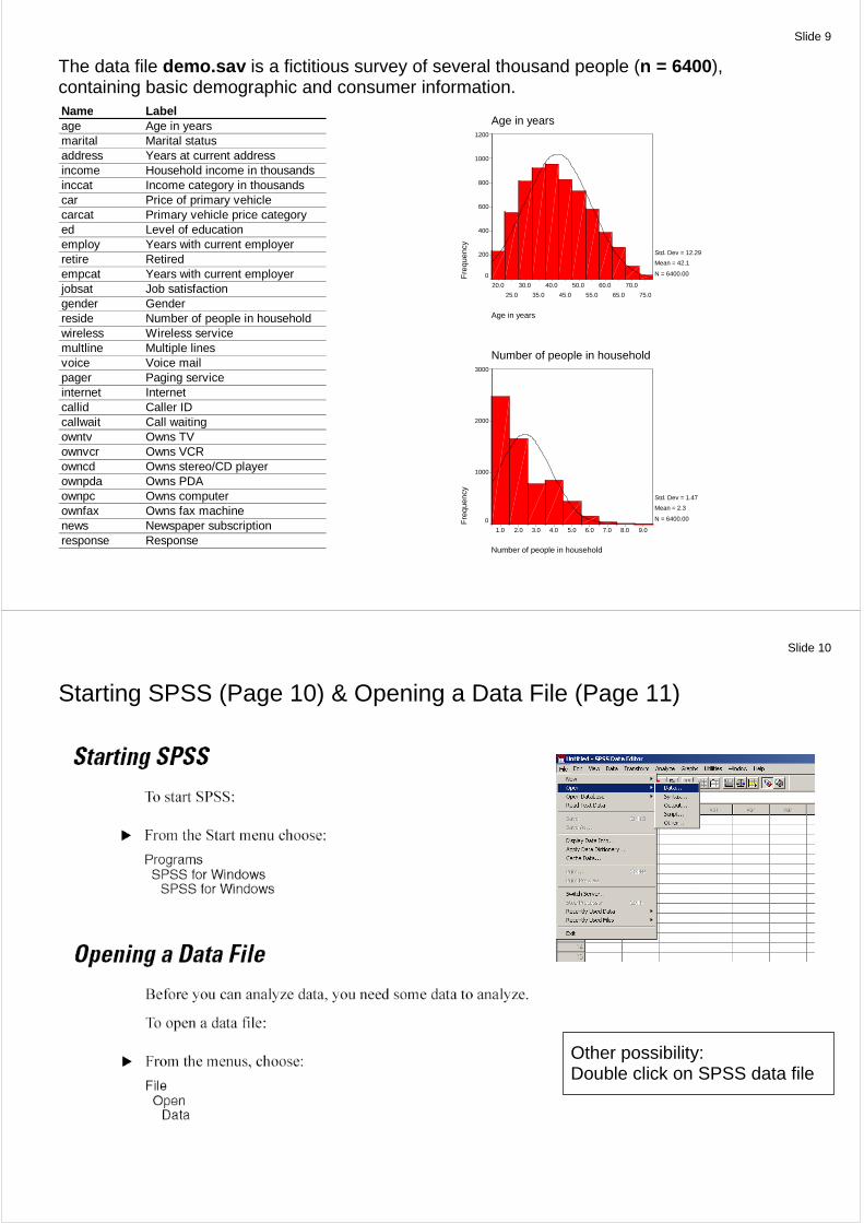
The data file demo.sav is a fictitious survey of several thousand people (n = 6400), containing basic demographic and consumer information. Name Labelage Age in yearsmarital Marital statusaddress Years at current addressincome Household income in thousandsinccat Income category in thousandscar Price of primary vehiclecarcat Primary vehicle price categoryed Level of educationemploy Years with current employerretire Retiredempcat Years with current employerjobsat Job satisfactiongender Genderreside Number of people in householdwireless Wireless servicemultline Multiple linesvoice Voice mailpager Paging serviceinternet Internetcallid Caller IDcallwait Call waitingowntv Owns TVownvcr Owns VCRowncd Owns stereo/CD playerownpda Owns PDAownpc Owns computerownfax Owns fax machinenews Newspaper subscriptionresponse Response
Age in years
75.0
70.0
65.0
60.0
55.0
50.0
45.0
40.0
35.0
30.0
25.0
20.0
Age in years
Fre
quen
cy
1200
1000
800
600
400
200
0
Std. Dev = 12.29
Mean = 42.1
N = 6400.00
Number of people in household
9.08.07.06.05.04.03.02.01.0
Number of people in household
Fre
quen
cy
3000
2000
1000
0
Std. Dev = 1.47
Mean = 2.3
N = 6400.00
Slide 10
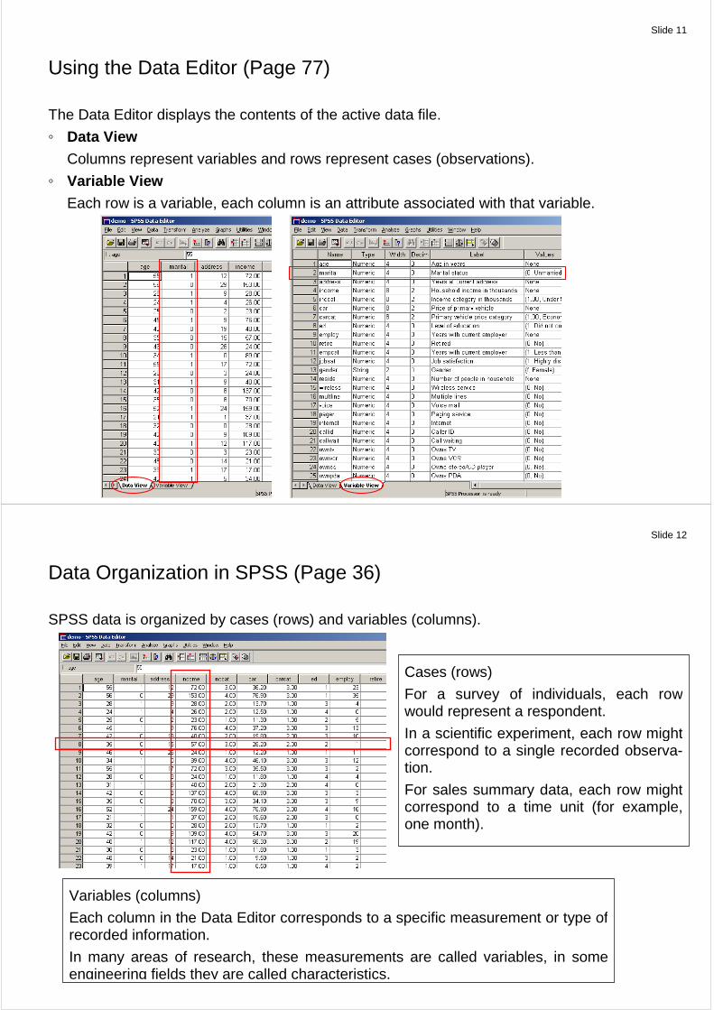
Starting SPSS (Page 10) & Opening a Data File (Page 11)
Other possibility: Double click on SPSS data file
Slide 11
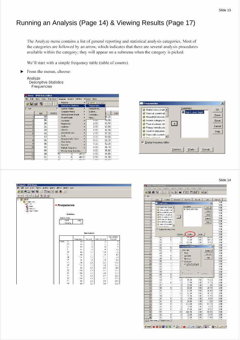
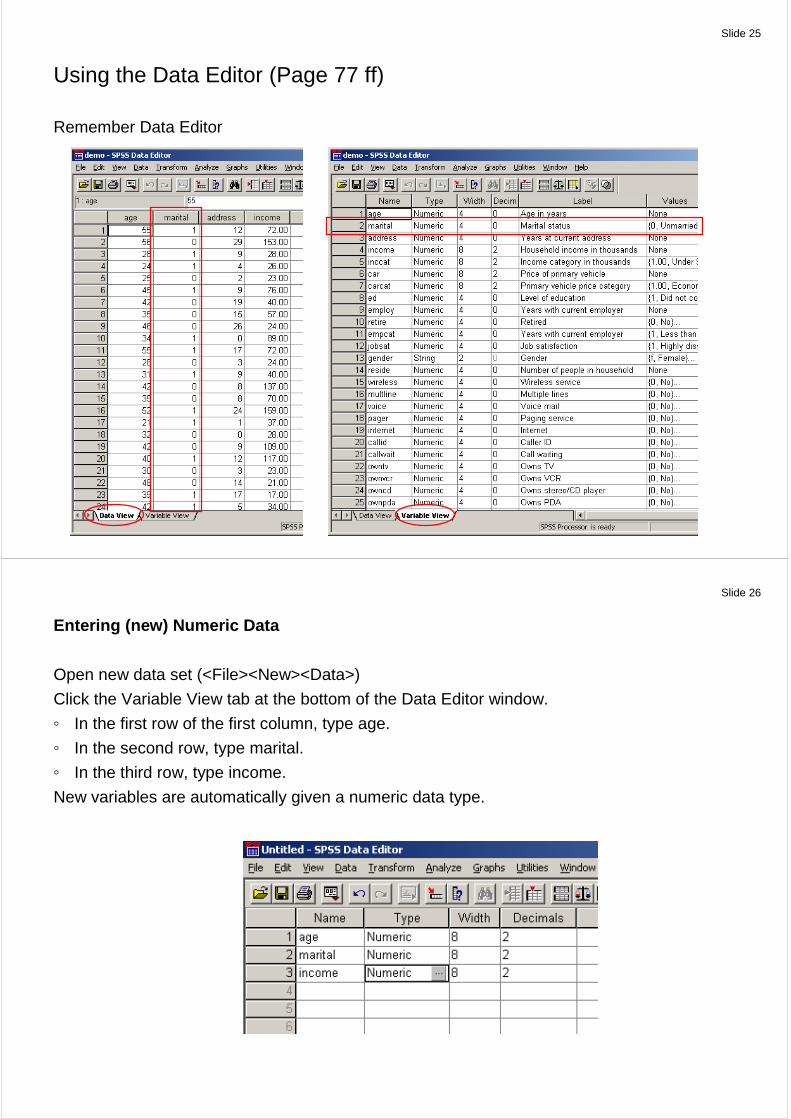
Using the Data Editor (Page 77)
The Data Editor displays the contents of the active data file.
Data View
Columns represent variables and rows represent cases (observations).
Variable View
Each row is a variable, each column is an attribute associated with that variable.
Slide 12
Data Organization in SPSS (Page 36)
SPSS data is organized by cases (rows) and variables (columns).
Cases (rows)
For a survey of individuals, each row would represent a respondent.
In a scientific experiment, each row might correspond to a single recorded observa-tion.
For sales summary data, each row might correspond to a time unit (for example, one month).
Variables (columns)
Each column in the Data Editor corresponds to a specific measurement or type of recorded information.
In many areas of research, these measurements are called variables, in some engineering fields they are called characteristics.
Slide 13
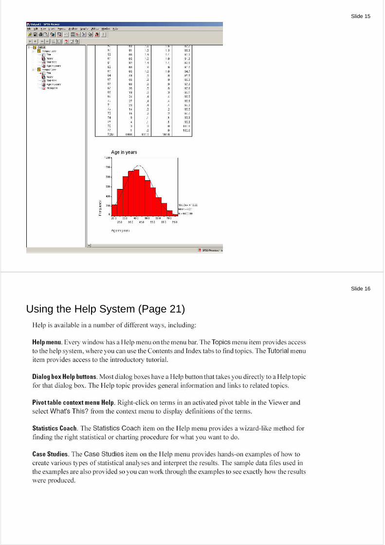
Running an Analysis (Page 14) & Viewing Results (Page 17)
Slide 14
Slide 15
Slide 16
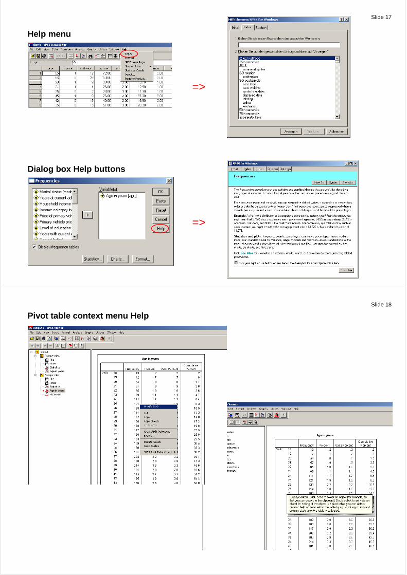
Using the Help System (Page 21)
Slide 17
Help menu
Dialog box Help buttons
=>
=>
Slide 18
Pivot table context menu Help
Slide 19
Choices in Entering Data (Page 38)
There are various methods of entering the data values.
SPSS Data Editor
Spreadsheet programs (e.g. Excel)
Database programs (e.g. Access)
For high-volume processing of surveys, you might consider scanning the survey responses.
Slide 20
Reading Data (Page 41)
Data can be imported from a number of different sources.
Reading an SPSS Data File
SPSS data files, which have a *.sav file extension, containing your saved data.
Reading Data from Spreadsheets
Rather than typing all your data directly into the Data Editor, you can read data from applica-tions like Microsoft Excel. You can also read column headings as variable names.
Reading Data from a Text File
Text files are common source of data. Many spreadsheet programs and databases can save their contents in one of many text file formats.
Comma or tab delimited files refer to rows of data that use commas or tabs to indicate each variable.
Reading Data from a Database (not shown in this course)
Data from database sources are easily imported using the Database Wizard.
Slide 21
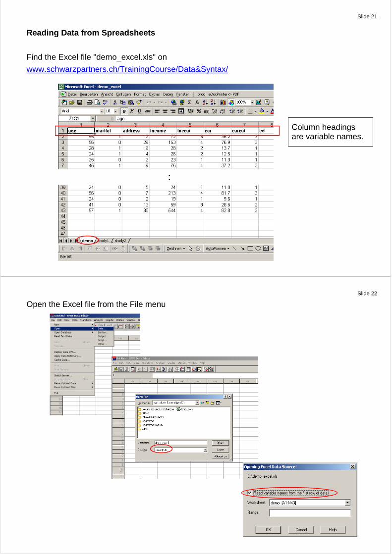
Reading Data from Spreadsheets
Find the Excel file "demo_excel.xls" on
www.schwarzpartners.ch/TrainingCourse/Data&Syntax/
:
Column headings are variable names.
Slide 22
Open the Excel file from the File menu
Slide 23
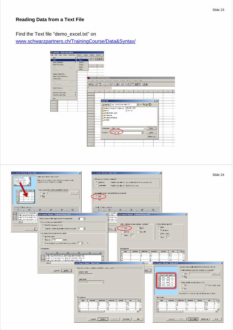
Reading Data from a Text File
Find the Text file "demo_excel.txt" on
www.schwarzpartners.ch/TrainingCourse/Data&Syntax/
Slide 24
Slide 25
Using the Data Editor (Page 77 ff)
Remember Data Editor
Slide 26
Entering (new) Numeric Data
Open new data set (<File><New><Data>)
Click the Variable View tab at the bottom of the Data Editor window.
In the first row of the first column, type age.
In the second row, type marital.
In the third row, type income.
New variables are automatically given a numeric data type.
Slide 27
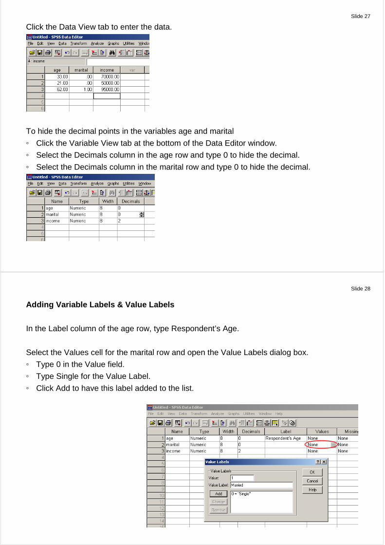
Click the Data View tab to enter the data.
To hide the decimal points in the variables age and marital
Click the Variable View tab at the bottom of the Data Editor window.
Select the Decimals column in the age row and type 0 to hide the decimal.
Select the Decimals column in the marital row and type 0 to hide the decimal.
Slide 28
Adding Variable Labels & Value Labels
In the Label column of the age row, type Respondent’s Age.
Select the Values cell for the marital row and open the Value Labels dialog box.
Type 0 in the Value field.
Type Single for the Value Label.
Click Add to have this label added to the list.
Slide 29
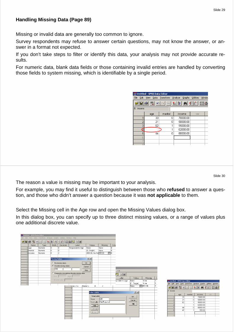
Handling Missing Data (Page 89)
Missing or invalid data are generally too common to ignore.
Survey respondents may refuse to answer certain questions, may not know the answer, or an-swer in a format not expected.
If you don’t take steps to filter or identify this data, your analysis may not provide accurate re-sults.
For numeric data, blank data fields or those containing invalid entries are handled by converting those fields to system missing, which is identifiable by a single period.
Slide 30
The reason a value is missing may be important to your analysis.
For example, you may find it useful to distinguish between those who refused to answer a ques-tion, and those who didn’t answer a question because it was not applicable to them.
Select the Missing cell in the Age row and open the Missing Values dialog box.
In this dialog box, you can specify up to three distinct missing values, or a range of values plus one additional discrete value.
Slide 31
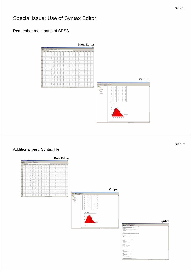
Special issue: Use of Syntax Editor
Remember main parts of SPSS
Output
Data Editor
Slide 32
Additional part: Syntax file
Output
Syntax
Data Editor

Slide 33
Open new syntax file via Menu <File> <Open> <New> <Syntax>
Output
Syntax
Data Editor
Slide 34
Running an Analysis via Menu
Example <Analyze><Frequencies>
Output
Data Editor
Slide 35
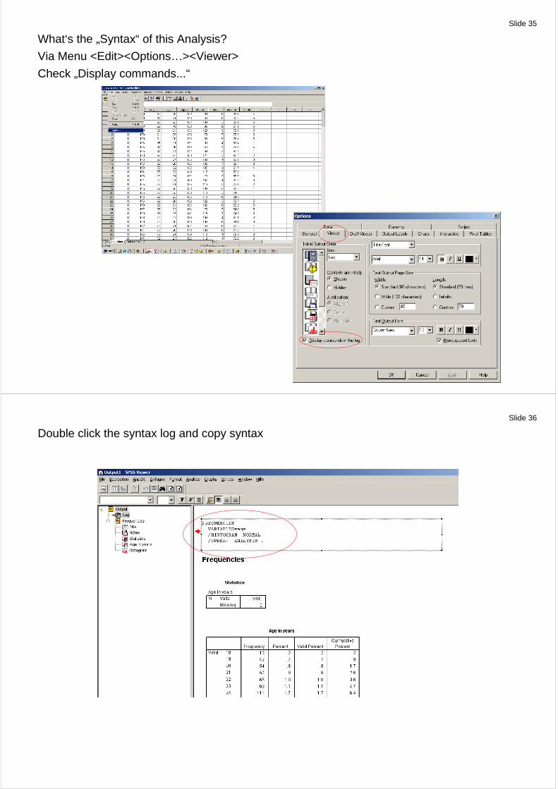
What‘s the „Syntax“ of this Analysis?
Via Menu <Edit><Options…><Viewer>
Check „Display commands...“
Slide 36
Double click the syntax log and copy syntax
Slide 37
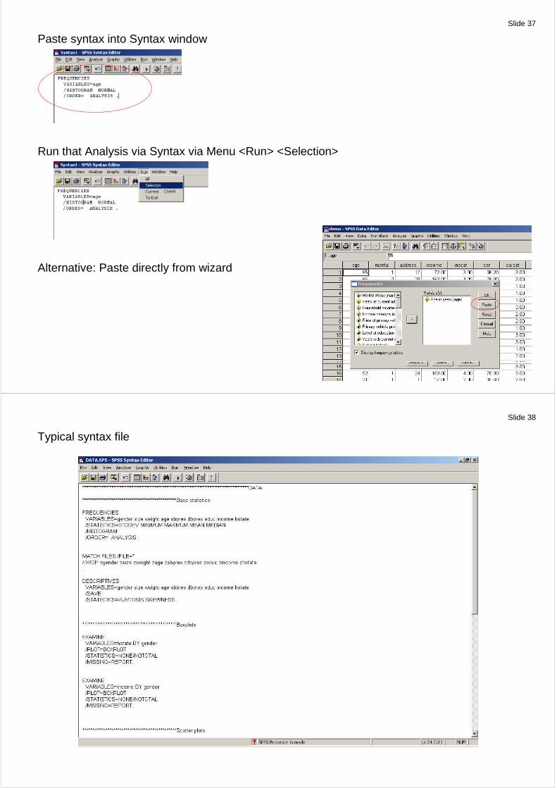
Paste syntax into Syntax window
Run that Analysis via Syntax via Menu <Run> <Selection>
Alternative: Paste directly from wizard
Slide 38
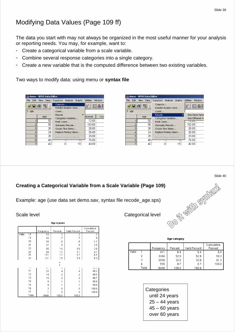
Typical syntax file
Slide 39
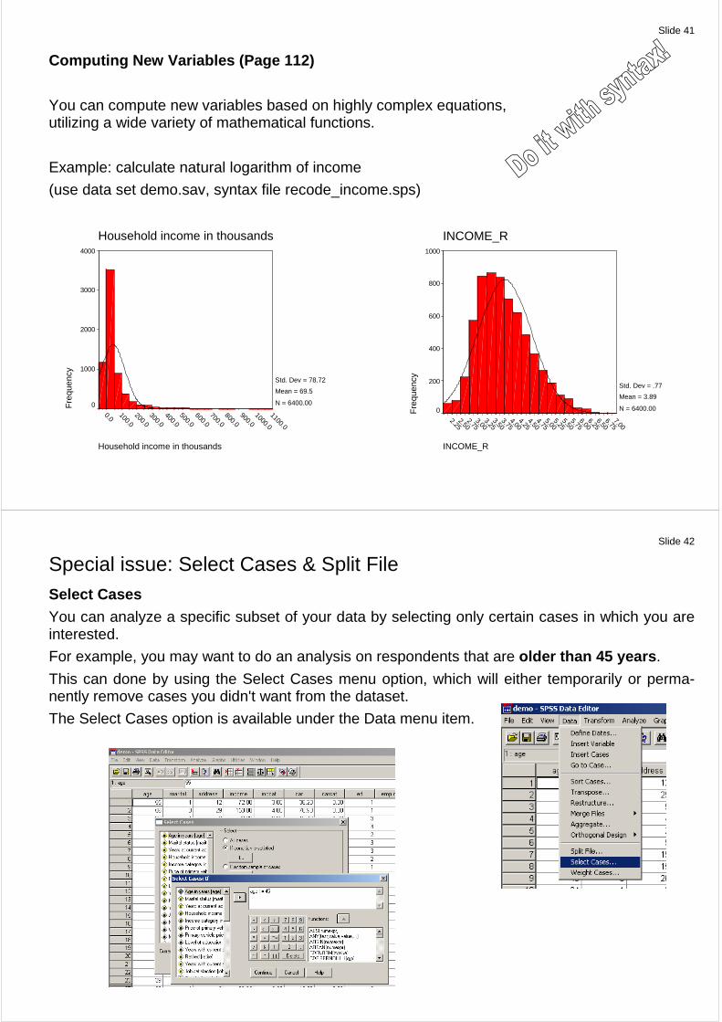
Modifying Data Values (Page 109 ff)
The data you start with may not always be organized in the most useful manner for your analysis or reporting needs. You may, for example, want to:
Create a categorical variable from a scale variable.
Combine several response categories into a single category.
Create a new variable that is the computed difference between two existing variables.
Two ways to modify data: using menu or syntax file
Slide 40
Creating a Categorical Variable from a Scale Variab le (Page 109)
Example: age (use data set demo.sav, syntax file recode_age.sps)
Scale level Categorical level
:
Categories until 24 years 25 – 44 years 45 – 60 years over 60 years
Slide 41
Computing New Variables (Page 112)
You can compute new variables based on highly complex equations, utilizing a wide variety of mathematical functions.
Example: calculate natural logarithm of income
(use data set demo.sav, syntax file recode_income.sps)
Household income in thousands
1100.0
1000.0
900.0800.0
700.0600.0
500.0400.0
300.0200.0
100.00.0
Household income in thousands
Fre
quen
cy
4000
3000
2000
1000
0
Std. Dev = 78.72
Mean = 69.5
N = 6400.00
INCOME_R
7.006.75
6.506.25
6.005.75
5.505.25
5.004.75
4.504.25
4.003.75
3.503.25
3.002.75
2.502.25
INCOME_R
Fre
quen
cy
1000
800
600
400
200
0
Std. Dev = .77
Mean = 3.89
N = 6400.00
Slide 42
Special issue: Select Cases & Split File Select Cases You can analyze a specific subset of your data by selecting only certain cases in which you are interested.
For example, you may want to do an analysis on respondents that are older than 45 years .
This can done by using the Select Cases menu option, which will either temporarily or perma-nently remove cases you didn't want from the dataset.
The Select Cases option is available under the Data menu item.
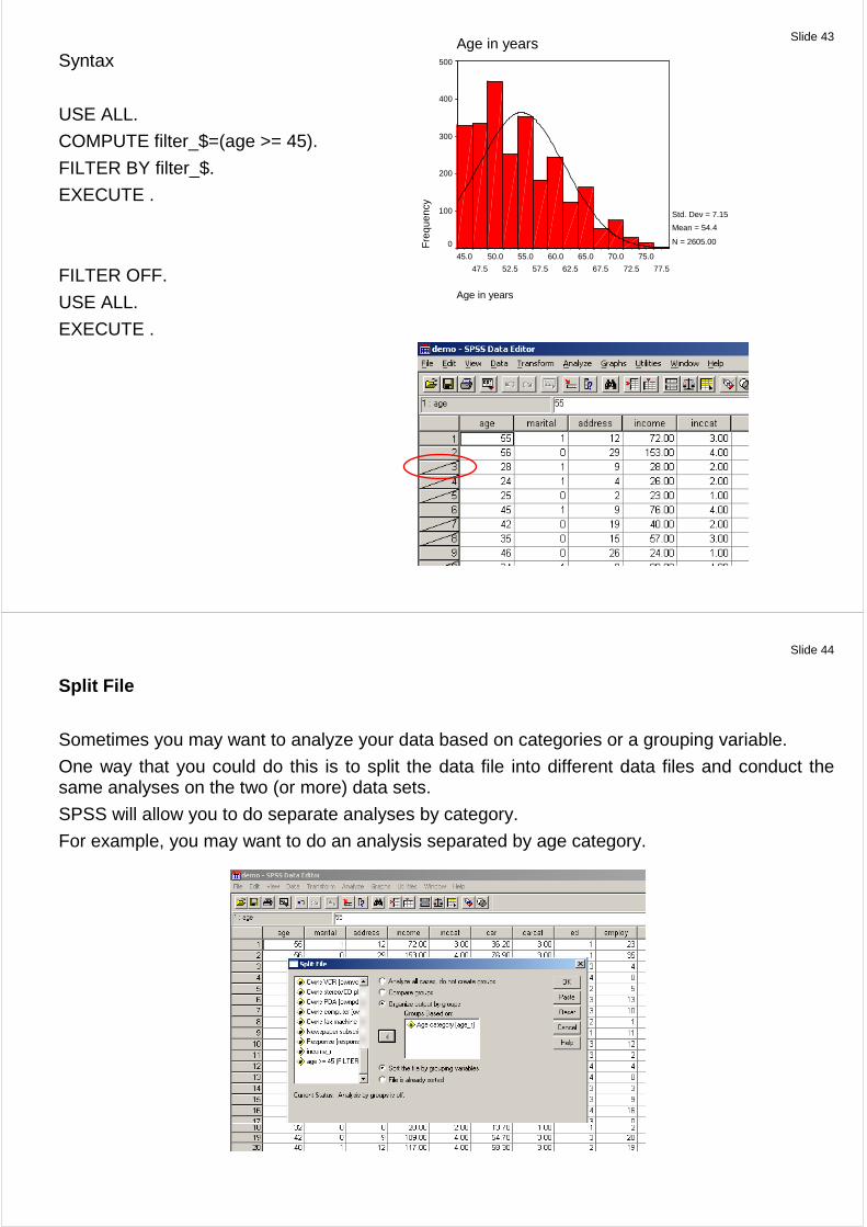
Slide 43
Syntax
USE ALL.
COMPUTE filter_$=(age >= 45).
FILTER BY filter_$.
EXECUTE .
FILTER OFF.
USE ALL.
EXECUTE .
Age in years
77.5
75.0
72.5
70.0
67.5
65.0
62.5
60.0
57.5
55.0
52.5
50.0
47.5
45.0
Age in years
Fre
quen
cy
500
400
300
200
100
0
Std. Dev = 7.15
Mean = 54.4
N = 2605.00
Slide 44
Split File
Sometimes you may want to analyze your data based on categories or a grouping variable.
One way that you could do this is to split the data file into different data files and conduct the same analyses on the two (or more) data sets.
SPSS will allow you to do separate analyses by category.
For example, you may want to do an analysis separated by age category.
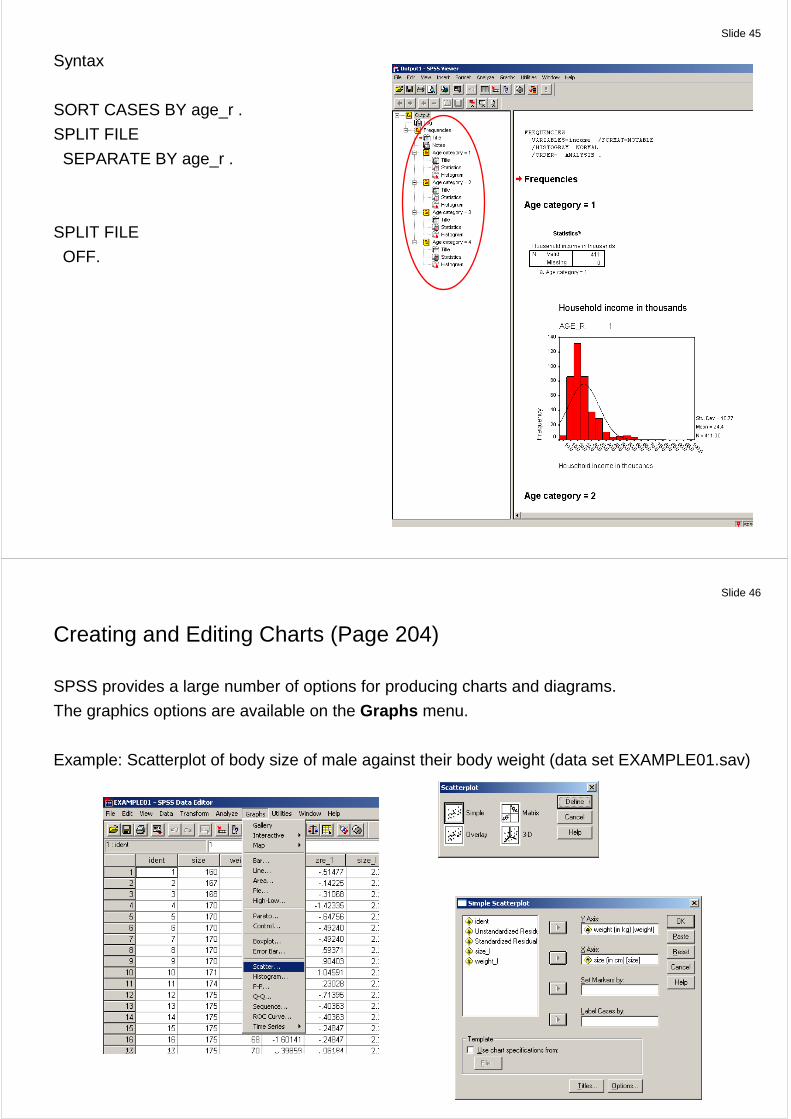
Slide 45
Syntax
SORT CASES BY age_r .
SPLIT FILE
SEPARATE BY age_r .
SPLIT FILE
OFF.
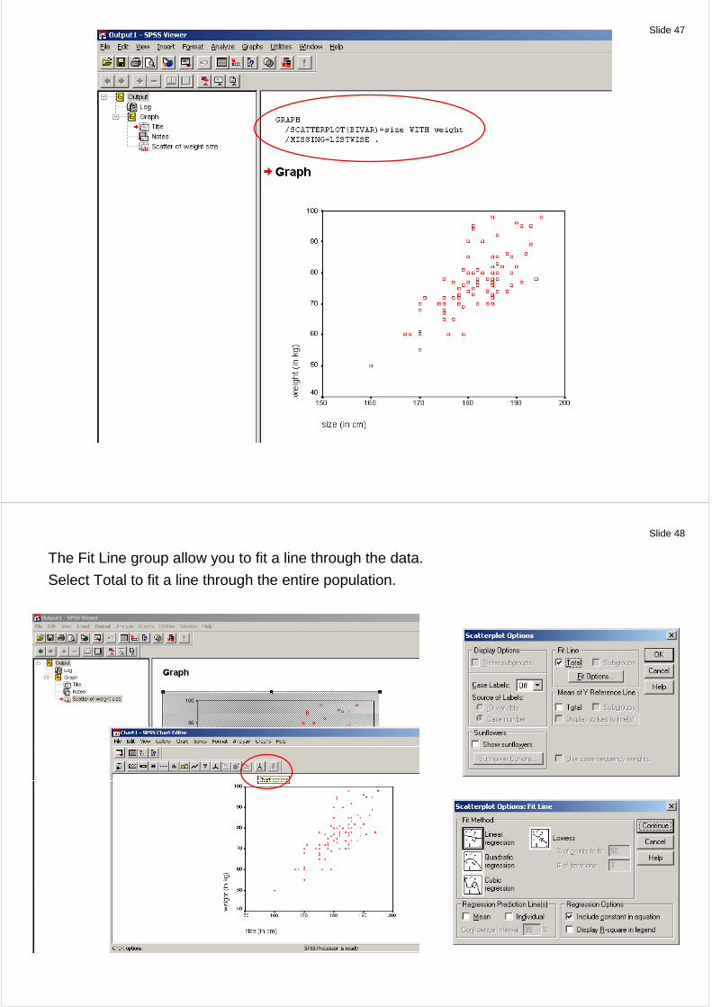
Slide 46
Creating and Editing Charts (Page 204)
SPSS provides a large number of options for producing charts and diagrams.
The graphics options are available on the Graphs menu.
Example: Scatterplot of body size of male against their body weight (data set EXAMPLE01.sav)
Slide 47
Slide 48
The Fit Line group allow you to fit a line through the data.
Select Total to fit a line through the entire population.
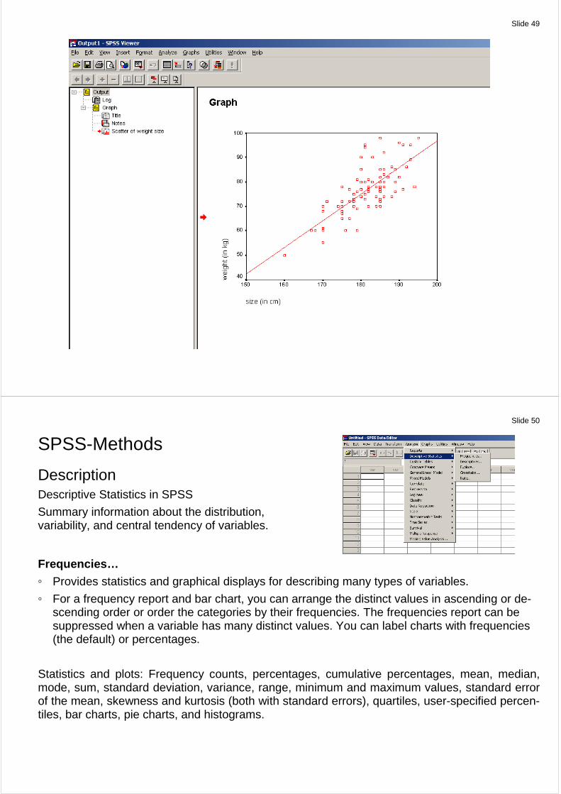
Slide 49
Slide 50
SPSS-Methods
Description Descriptive Statistics in SPSS
Summary information about the distribution, variability, and central tendency of variables.
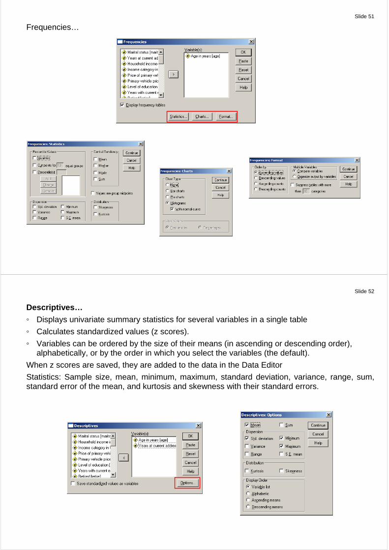
Frequencies… Provides statistics and graphical displays for describing many types of variables.
For a frequency report and bar chart, you can arrange the distinct values in ascending or de-scending order or order the categories by their frequencies. The frequencies report can be suppressed when a variable has many distinct values. You can label charts with frequencies (the default) or percentages.
Statistics and plots: Frequency counts, percentages, cumulative percentages, mean, median, mode, sum, standard deviation, variance, range, minimum and maximum values, standard error of the mean, skewness and kurtosis (both with standard errors), quartiles, user-specified percen-tiles, bar charts, pie charts, and histograms.
Slide 51
Frequencies…
Slide 52
Descriptives… Displays univariate summary statistics for several variables in a single table
Calculates standardized values (z scores).
Variables can be ordered by the size of their means (in ascending or descending order), alphabetically, or by the order in which you select the variables (the default).
When z scores are saved, they are added to the data in the Data Editor
Statistics: Sample size, mean, minimum, maximum, standard deviation, variance, range, sum, standard error of the mean, and kurtosis and skewness with their standard errors.
Slide 53
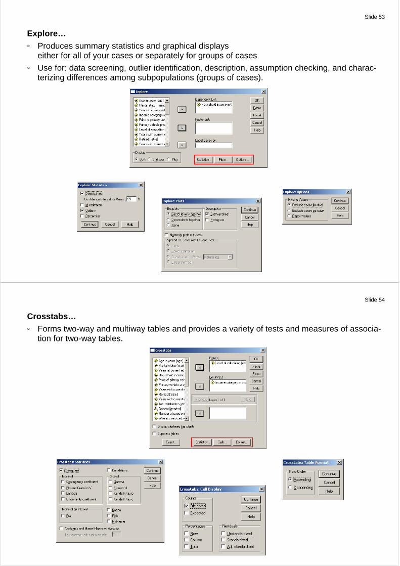
Explore… Produces summary statistics and graphical displays
either for all of your cases or separately for groups of cases
Use for: data screening, outlier identification, description, assumption checking, and charac-terizing differences among subpopulations (groups of cases).
Slide 54
Crosstabs… Forms two-way and multiway tables and provides a variety of tests and measures of associa-
tion for two-way tables.
Slide 55
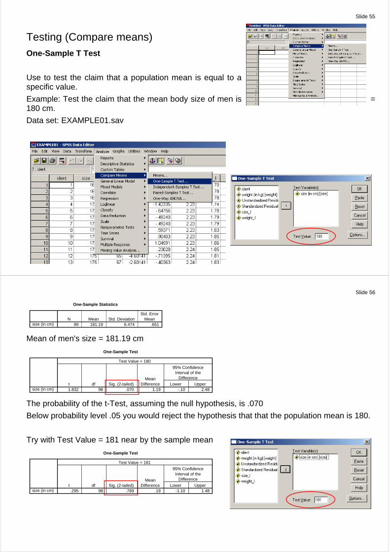
Testing (Compare means) One-Sample T Test
Use to test the claim that a population mean is equal to a specific value.
Example: Test the claim that the mean body size of men is = 180 cm.
Data set: EXAMPLE01.sav
Slide 56
One-Sample Statistics
99 181.19 6.474 .651size (in cm)N Mean Std. Deviation
Std. ErrorMean
Mean of men's size = 181.19 cm
One-Sample Test
1.832 98 .070 1.19 -.10 2.48size (in cm)t df Sig. (2-tailed)
MeanDifference Lower Upper
95% ConfidenceInterval of the
Difference
Test Value = 180
The probability of the t-Test, assuming the null hypothesis, is .070
Below probability level .05 you would reject the hypothesis that that the population mean is 180.
Try with Test Value = 181 near by the sample mean
One-Sample Test
.295 98 .769 .19 -1.10 1.48size (in cm)t df Sig. (2-tailed)
MeanDifference Lower Upper
95% ConfidenceInterval of the
Difference
Test Value = 181
Slide 57
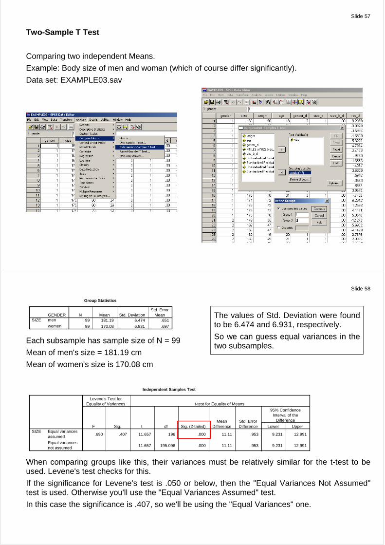
Two-Sample T Test
Comparing two independent Means.
Example: Body size of men and woman (which of course differ significantly).
Data set: EXAMPLE03.sav
Slide 58
Group Statistics
99 181.19 6.474 .651
99 170.08 6.931 .697
GENDERmen
women
SIZEN Mean Std. Deviation
Std. ErrorMean
Each subsample has sample size of N = 99
Mean of men's size = 181.19 cm
Mean of women's size is 170.08 cm
Independent Samples Test
.690 .407 11.657 196 .000 11.11 .953 9.231 12.991
11.657 195.096 .000 11.11 .953 9.231 12.991
Equal variancesassumed
Equal variancesnot assumed
SIZEF Sig.
Levene's Test forEquality of Variances
t df Sig. (2-tailed)Mean
DifferenceStd. ErrorDifference Lower Upper
95% ConfidenceInterval of the
Difference
t-test for Equality of Means
When comparing groups like this, their variances must be relatively similar for the t-test to be used. Levene's test checks for this.
If the significance for Levene's test is .050 or below, then the "Equal Variances Not Assumed" test is used. Otherwise you'll use the "Equal Variances Assumed" test.
In this case the significance is .407, so we'll be using the "Equal Variances" one.
The values of Std. Deviation were found to be 6.474 and 6.931, respectively.
So we can guess equal variances in the two subsamples.
Slide 59
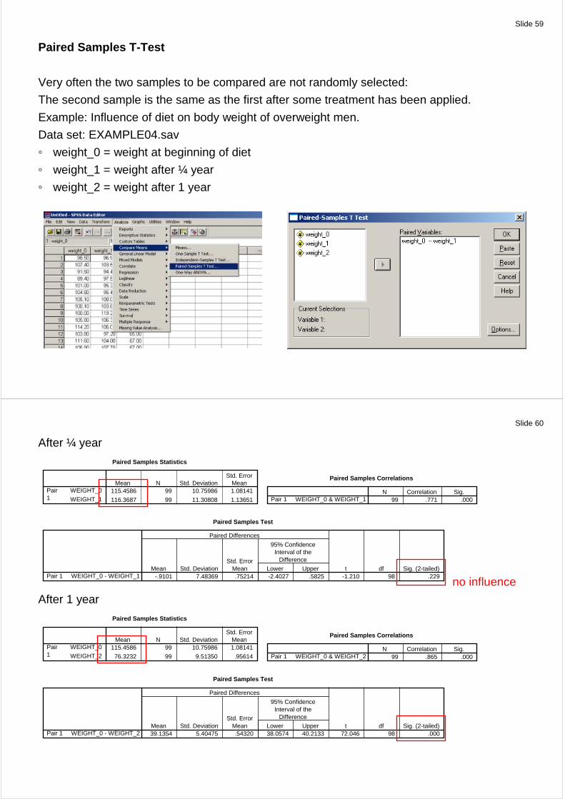
Paired Samples T-Test
Very often the two samples to be compared are not randomly selected:
The second sample is the same as the first after some treatment has been applied.
Example: Influence of diet on body weight of overweight men.
Data set: EXAMPLE04.sav
weight_0 = weight at beginning of diet
weight_1 = weight after ¼ year
weight_2 = weight after 1 year
Slide 60
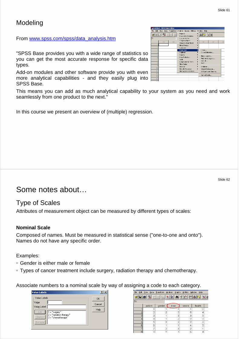
After ¼ year
Paired Samples Statistics
115.4586 99 10.75986 1.08141
116.3687 99 11.30808 1.13651
WEIGHT_0
WEIGHT_1
Pair1
Mean N Std. DeviationStd. Error
MeanPaired Samples Correlations
99 .771 .000WEIGHT_0 & WEIGHT_1Pair 1N Correlation Sig.
Paired Samples Test
-.9101 7.48369 .75214 -2.4027 .5825 -1.210 98 .229WEIGHT_0 - WEIGHT_1Pair 1Mean Std. Deviation
Std. ErrorMean Lower Upper
95% ConfidenceInterval of the
Difference
Paired Differences
t df Sig. (2-tailed)
no influence
After 1 year
Paired Samples Statistics
115.4586 99 10.75986 1.08141
76.3232 99 9.51350 .95614
WEIGHT_0
WEIGHT_2
Pair1
Mean N Std. DeviationStd. Error
MeanPaired Samples Correlations
99 .865 .000WEIGHT_0 & WEIGHT_2Pair 1N Correlation Sig.
Paired Samples Test
39.1354 5.40475 .54320 38.0574 40.2133 72.046 98 .000WEIGHT_0 - WEIGHT_2Pair 1Mean Std. Deviation
Std. ErrorMean Lower Upper
95% ConfidenceInterval of the
Difference
Paired Differences
t df Sig. (2-tailed)
Slide 61
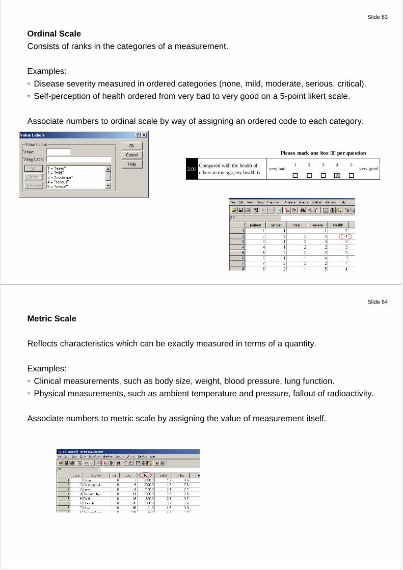
Modeling
From www.spss.com/spss/data_analysis.htm
"SPSS Base provides you with a wide range of statistics so you can get the most accurate response for specific data types.
Add-on modules and other software provide you with even more analytical capabilities - and they easily plug into SPSS Base.
This means you can add as much analytical capability to your system as you need and work seamlessly from one product to the next."
In this course we present an overview of (multiple) regression.
Slide 62
Some notes about…
Type of Scales Attributes of measurement object can be measured by different types of scales:
Nominal Scale Composed of names. Must be measured in statistical sense ("one-to-one and onto"). Names do not have any specific order.
Examples:
Gender is either male or female
Types of cancer treatment include surgery, radiation therapy and chemotherapy.
Associate numbers to a nominal scale by way of assigning a code to each category.
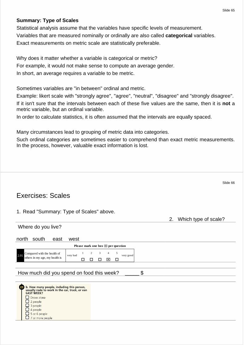
Slide 63
Ordinal Scale Consists of ranks in the categories of a measurement.
Examples:
Disease severity measured in ordered categories (none, mild, moderate, serious, critical).
Self-perception of health ordered from very bad to very good on a 5-point likert scale.
Associate numbers to ordinal scale by way of assigning an ordered code to each category.
1 2 3 4 5
� � � �
Please mark one box per question
2.01Compared with the health of others in my age, my health is
very bad very good
Slide 64
Metric Scale
Reflects characteristics which can be exactly measured in terms of a quantity.
Examples:
Clinical measurements, such as body size, weight, blood pressure, lung function.
Physical measurements, such as ambient temperature and pressure, fallout of radioactivity.
Associate numbers to metric scale by assigning the value of measurement itself.
Slide 65
Summary: Type of Scales Statistical analysis assume that the variables have specific levels of measurement.
Variables that are measured nominally or ordinally are also called categorical variables.
Exact measurements on metric scale are statistically preferable.
Why does it matter whether a variable is categorical or metric?
For example, it would not make sense to compute an average gender.
In short, an average requires a variable to be metric.
Sometimes variables are "in between" ordinal and metric.
Example: likert scale with "strongly agree", "agree", "neutral", "disagree" and "strongly disagree".
If it isn't sure that the intervals between each of these five values are the same, then it is not a metric variable, but an ordinal variable.
In order to calculate statistics, it is often assumed that the intervals are equally spaced.
Many circumstances lead to grouping of metric data into categories.
Such ordinal categories are sometimes easier to comprehend than exact metric measurements. In the process, however, valuable exact information is lost.
Slide 66
Exercises: Scales
1. Read "Summary: Type of Scales" above.
2. Which type of scale?
Where do you live? � � � � north south east west
1 2 3 4 5
� � � �
Please mark one box per question
2.01Compared with the health of others in my age, my health is
very bad very good
How much did you spend on food this week? _____ $
Slide 67
Slide 68
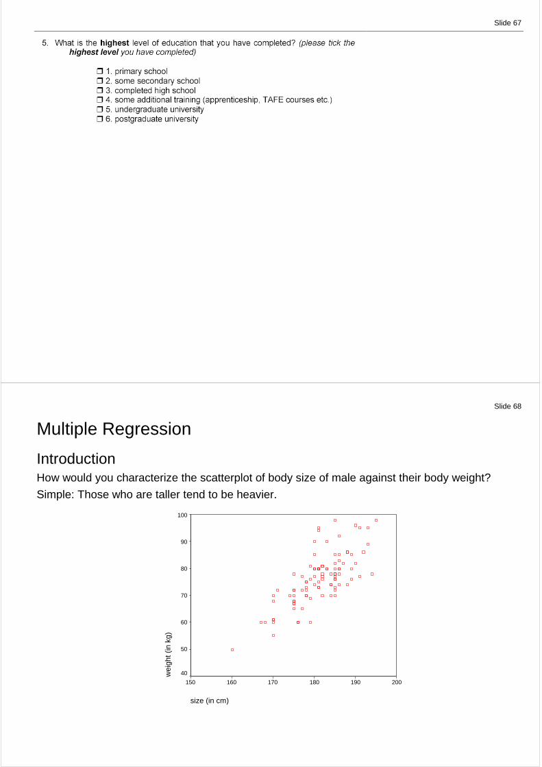
Multiple Regression
Introduction How would you characterize the scatterplot of body size of male against their body weight?
Simple: Those who are taller tend to be heavier.
size (in cm)
200190180170160150
wei
ght (
in k
g)
100
90
80
70
60
50
40
Slide 69
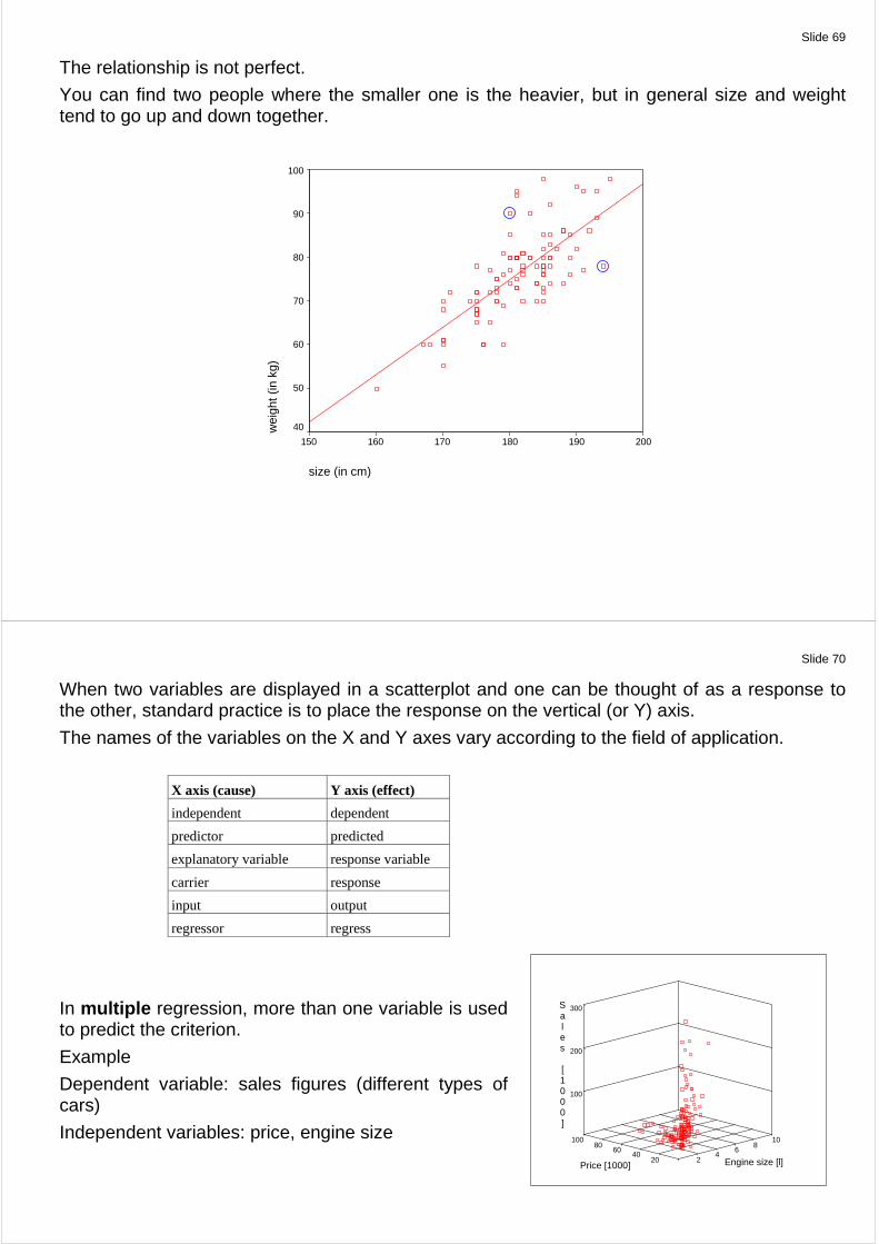
The relationship is not perfect.
You can find two people where the smaller one is the heavier, but in general size and weight tend to go up and down together.
size (in cm)
200190180170160150
wei
ght (
in k
g)
100
90
80
70
60
50
40
Slide 70
Sales [1000]
10100
100
880
200
300
660
Price [1000] Engine size [l]440
220
When two variables are displayed in a scatterplot and one can be thought of as a response to the other, standard practice is to place the response on the vertical (or Y) axis.
The names of the variables on the X and Y axes vary according to the field of application.
X axis (cause) Y axis (effect)
independent dependent
predictor predicted
explanatory variable response variable
carrier response
input output
regressor regress
In multiple regression, more than one variable is used to predict the criterion.
Example
Dependent variable: sales figures (different types of cars)
Independent variables: price, engine size
Slide 71
General purpose of (multiple) regression
Cause analysis : Learn more about the relationship between several independent variables and a dependent variable.
Example
Is there a model as a whole that describes the dependence between sales figures, price and engine size? How large is the influence of the price, how that of the engine size?
Impact analysis : Assess the impact of changing an independent variable to the value of de-pendent variable.
Example
If the price is increased, will sales volume decline and if it does, will it be more or less propor-tionate to the rise in price?
Time series analysis : Predict values of a time series, using either previous values of just that one series, or values from other series as well.
Example
How does sales volume vary in the next 6 months?
Slide 72
Key steps involved in using multiple regression 1. Formulation of the model Common sense should be your guide
Not too much variables
2. Estimation of the model Model estimation in SPSS (see below)
Interpretation of coefficients
3. Verification of the model
How much variation does the regression equation explain?
=> Coefficient of determination ("R squared")
Are the coefficients significant as a group ? (ie. Is the model significant?)
=> F-test
Test for individual regression coefficients
=> t-test (should be performed only if F-test is significant)
Slide 73
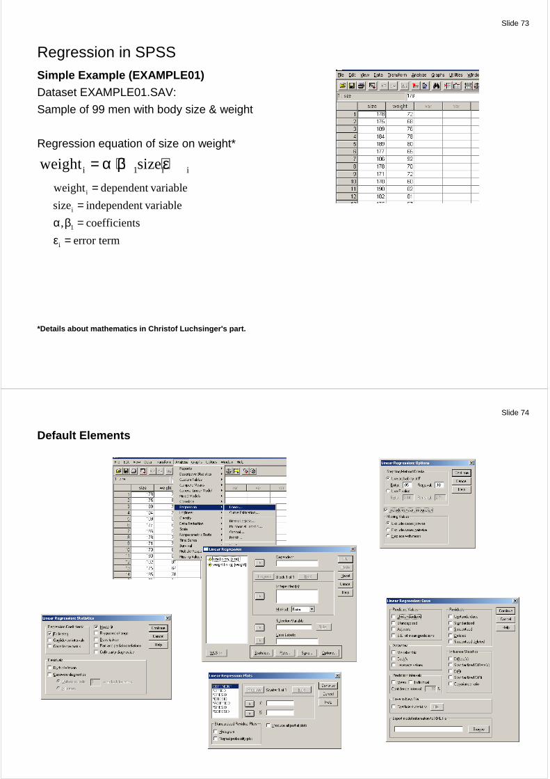
Regression in SPSS Simple Example (EXAMPLE01) Dataset EXAMPLE01.SAV:
Sample of 99 men with body size & weight
Regression equation of size on weight*
i 1 i iweight size= α + β + ε
i
i
1
i
weight dependent variable
size independent variable
, coefficients
error term
==
α β =ε =
*Details about mathematics in Christof Luchsinger's part.
Slide 74
Default Elements
Slide 75
size (in cm)
200180160140120100806040200
wei
ght (
in k
g)
100
80
60
40
20
0
-20
-40
-60
-80
-100
-120
-140
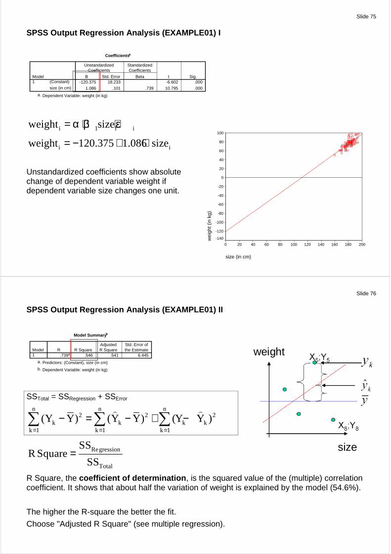
SPSS Output Regression Analysis (EXAMPLE01) I
Coefficients a
-120.375 18.233 -6.602 .000
1.086 .101 .739 10.795 .000
(Constant)
size (in cm)
Model1
B Std. Error
UnstandardizedCoefficients
Beta
StandardizedCoefficients
t Sig.
Dependent Variable: weight (in kg)a.
i 1 i iweight size= α + β + ε
i iweight 120.375 1.086 size= − + ⋅
Unstandardized coefficients show absolute change of dependent variable weight if dependent variable size changes one unit.
Slide 76
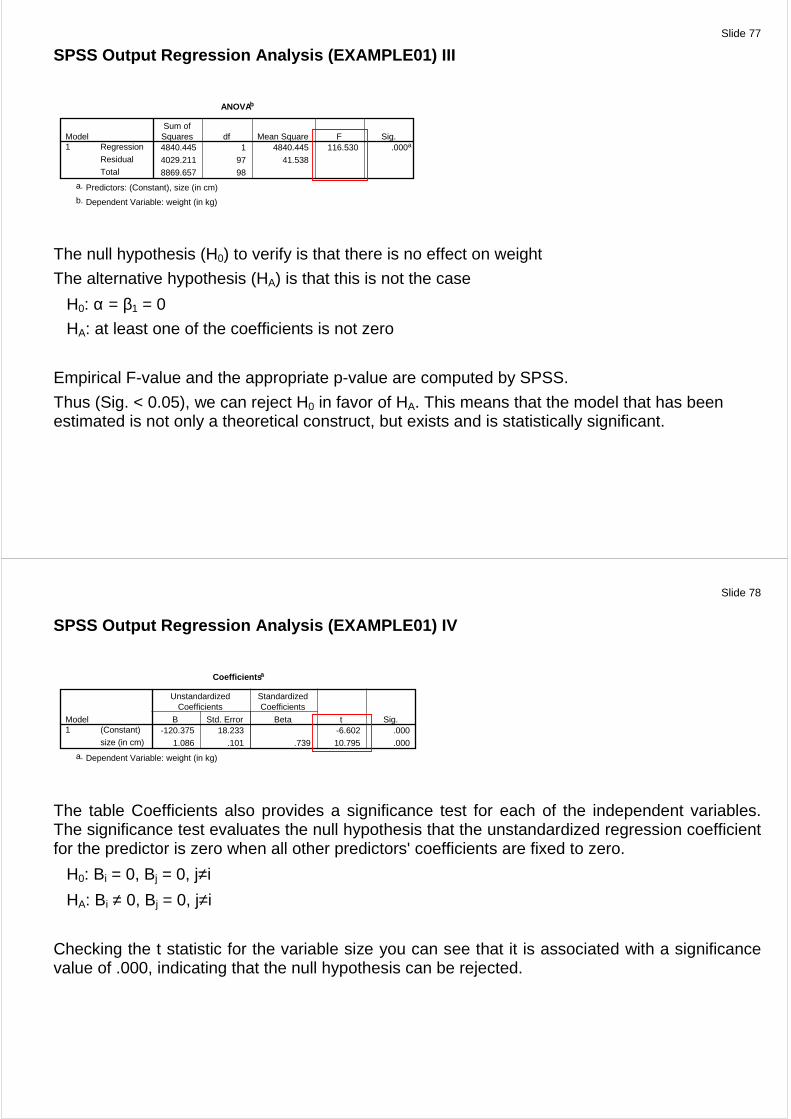
SPSS Output Regression Analysis (EXAMPLE01) II
Model Summary b
.739a .546 .541 6.445Model1
R R SquareAdjustedR Square
Std. Error ofthe Estimate
Predictors: (Constant), size (in cm)a.
Dependent Variable: weight (in kg)b.
SSTotal = SSRegression + SSError n n n
2 2 2k k k k
k 1 k 1 k 1
(Y Y) (Y Y) (Y Y )= = =
− = − + −∑ ∑ ∑⌢ ⌢
Regression
Total
SSR Square
SS=
R Square, the coefficient of determination , is the squared value of the (multiple) correlation coefficient. It shows that about half the variation of weight is explained by the model (54.6%).
The higher the R-square the better the fit.
Choose "Adjusted R Square" (see multiple regression).
weight
size
Slide 77
SPSS Output Regression Analysis (EXAMPLE01) III
ANOVAb
4840.445 1 4840.445 116.530 .000a
4029.211 97 41.538
8869.657 98
Regression
Residual
Total
Model1
Sum ofSquares df Mean Square F Sig.
Predictors: (Constant), size (in cm)a.
Dependent Variable: weight (in kg)b.
The null hypothesis (H0) to verify is that there is no effect on weight
The alternative hypothesis (HA) is that this is not the case
H0: α = β1 = 0
HA: at least one of the coefficients is not zero
Empirical F-value and the appropriate p-value are computed by SPSS.
Thus (Sig. < 0.05), we can reject H0 in favor of HA. This means that the model that has been estimated is not only a theoretical construct, but exists and is statistically significant.
Slide 78
SPSS Output Regression Analysis (EXAMPLE01) IV
Coefficients a
-120.375 18.233 -6.602 .000
1.086 .101 .739 10.795 .000
(Constant)
size (in cm)
Model1
B Std. Error
UnstandardizedCoefficients
Beta
StandardizedCoefficients
t Sig.
Dependent Variable: weight (in kg)a.
The table Coefficients also provides a significance test for each of the independent variables. The significance test evaluates the null hypothesis that the unstandardized regression coefficient for the predictor is zero when all other predictors' coefficients are fixed to zero.
H0: Bi = 0, Bj = 0, j≠i
HA: Bi ≠ 0, Bj = 0, j≠i
Checking the t statistic for the variable size you can see that it is associated with a significance value of .000, indicating that the null hypothesis can be rejected.
Slide 79
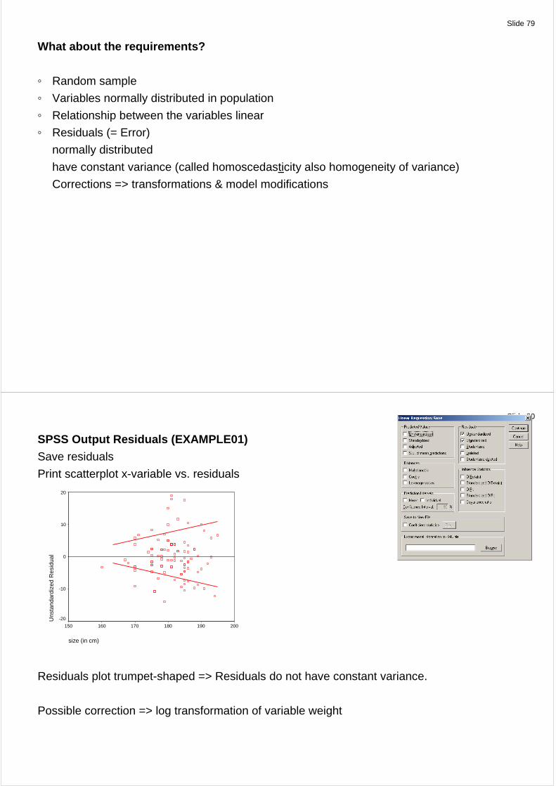
What about the requirements?
Random sample
Variables normally distributed in population
Relationship between the variables linear
Residuals (= Error)
normally distributed
have constant variance (called homoscedasticity also homogeneity of variance)
Corrections => transformations & model modifications
Slide 80
SPSS Output Residuals (EXAMPLE01) Save residuals
Print scatterplot x-variable vs. residuals
size (in cm)
200190180170160150
Uns
tand
ardi
zed
Res
idua
l
20
10
0
-10
-20
Residuals plot trumpet-shaped => Residuals do not have constant variance.
Possible correction => log transformation of variable weight
Slide 81
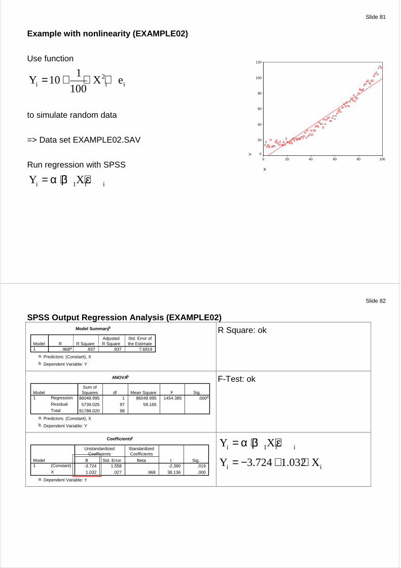
Example with nonlinearity (EXAMPLE02)
Use function
2i i i
1Y 10 X e
100= + ⋅ +
to simulate random data
=> Data set EXAMPLE02.SAV
Run regression with SPSS
i 1 i iY X= α + β + ε
X
100806040200
Y
120
100
80
60
40
20
0
Slide 82
SPSS Output Regression Analysis (EXAMPLE02) Model Summary b
.968a .937 .937 7.6919Model1
R R SquareAdjustedR Square
Std. Error ofthe Estimate
Predictors: (Constant), Xa.
Dependent Variable: Yb.
R Square: ok
ANOVAb
86048.995 1 86048.995 1454.385 .000a
5739.025 97 59.165
91788.020 98
Regression
Residual
Total
Model1
Sum ofSquares df Mean Square F Sig.
Predictors: (Constant), Xa.
Dependent Variable: Yb.
F-Test: ok
Coefficients a
-3.724 1.558 -2.390 .019
1.032 .027 .968 38.136 .000
(Constant)
X
Model1
B Std. Error
UnstandardizedCoefficients
Beta
StandardizedCoefficients
t Sig.
Dependent Variable: Ya.
i 1 i iY X= α + β + ε
i iY 3.724 1.032 X= − + ⋅
Slide 83
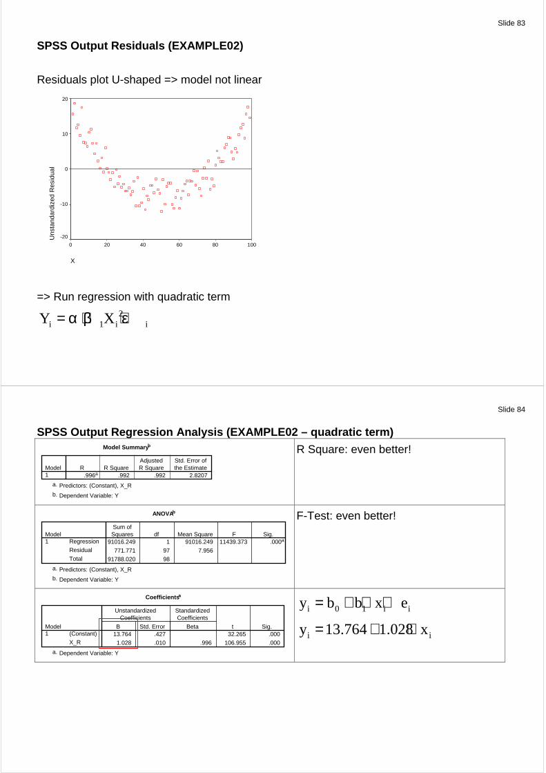
SPSS Output Residuals (EXAMPLE02)
Residuals plot U-shaped => model not linear
X
100806040200
Uns
tand
ardi
zed
Res
idua
l
20
10
0
-10
-20
=> Run regression with quadratic term 2
i 1 i iY X= α + β + ε
Slide 84
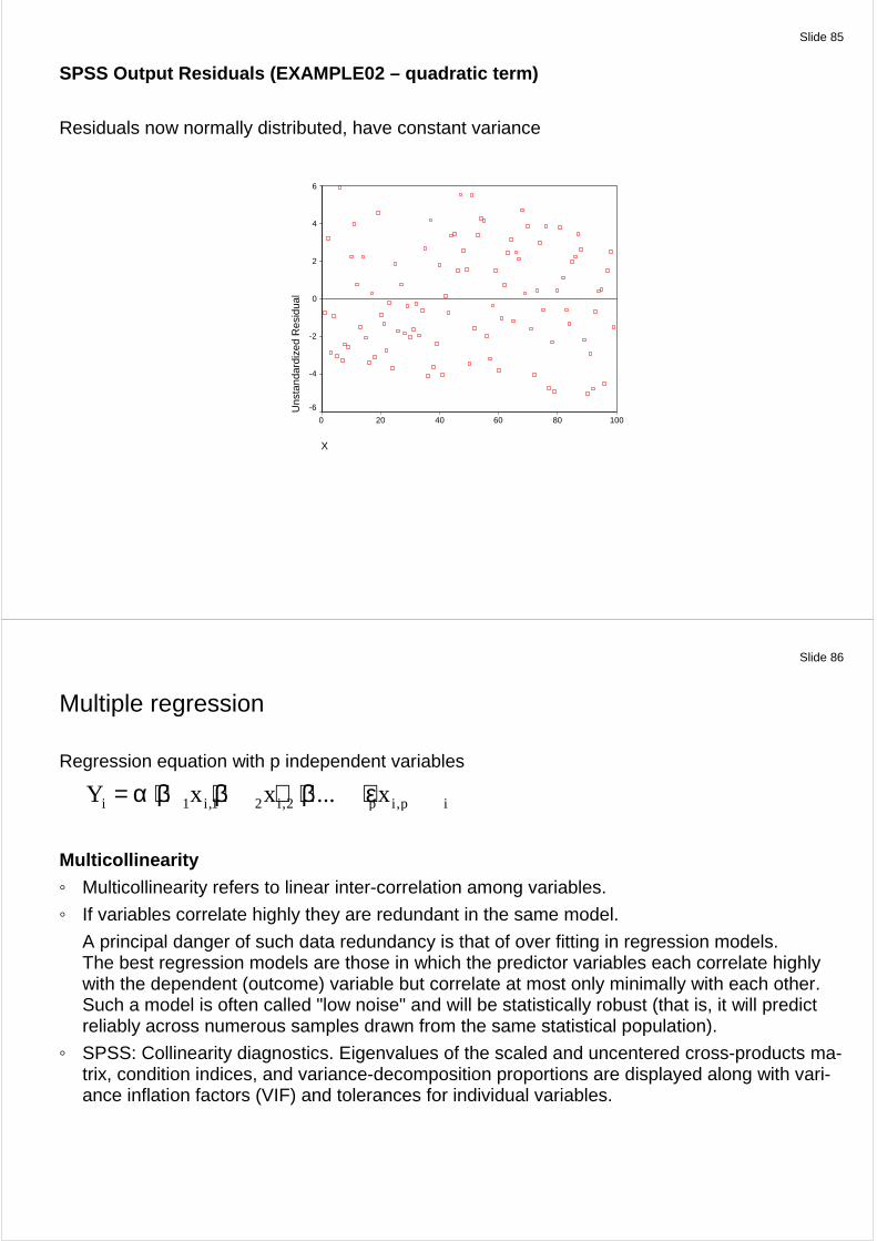
SPSS Output Regression Analysis (EXAMPLE02 – quadra tic term) Model Summary b
.996a .992 .992 2.8207Model1
R R SquareAdjustedR Square
Std. Error ofthe Estimate
Predictors: (Constant), X_Ra.
Dependent Variable: Yb.
R Square: even better!
ANOVAb
91016.249 1 91016.249 11439.373 .000a
771.771 97 7.956
91788.020 98
Regression
Residual
Total
Model1
Sum ofSquares df Mean Square F Sig.
Predictors: (Constant), X_Ra.
Dependent Variable: Yb.
F-Test: even better!
Coefficients a
13.764 .427 32.265 .000
1.028 .010 .996 106.955 .000
(Constant)
X_R
Model1
B Std. Error
UnstandardizedCoefficients
Beta
StandardizedCoefficients
t Sig.
Dependent Variable: Ya.
i 0 1 i iy b b x e= + ⋅ +
i iy 13.764 1.028 x= + ⋅
Slide 85
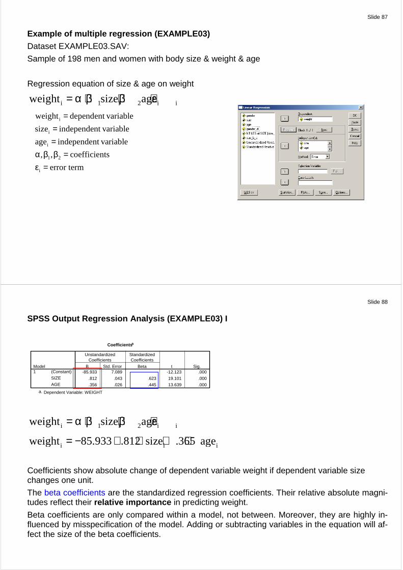
SPSS Output Residuals (EXAMPLE02 – quadratic term)
Residuals now normally distributed, have constant variance
X
100806040200
Uns
tand
ardi
zed
Res
idua
l
6
4
2
0
-2
-4
-6
Slide 86
Multiple regression
Regression equation with p independent variables
i 1 i,1 2 i,2 p i,p iY x x ... x= α + β + β + + β + ε
Multicollinearity
Multicollinearity refers to linear inter-correlation among variables.
If variables correlate highly they are redundant in the same model.
A principal danger of such data redundancy is that of over fitting in regression models. The best regression models are those in which the predictor variables each correlate highly
with the dependent (outcome) variable but correlate at most only minimally with each other. Such a model is often called "low noise" and will be statistically robust (that is, it will predict reliably across numerous samples drawn from the same statistical population).
SPSS: Collinearity diagnostics. Eigenvalues of the scaled and uncentered cross-products ma-trix, condition indices, and variance-decomposition proportions are displayed along with vari-ance inflation factors (VIF) and tolerances for individual variables.
Slide 87
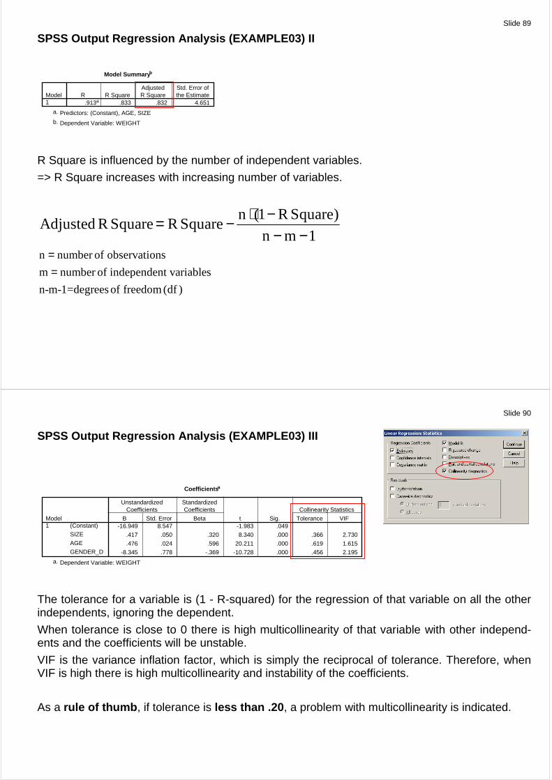
Example of multiple regression (EXAMPLE03) Dataset EXAMPLE03.SAV:
Sample of 198 men and women with body size & weight & age
Regression equation of size & age on weight
i 1 i 2 i iweight size age= α + β + β + ε
i
i
i
1 2
i
weight dependent variable
size independent variable
age independent variable
, , coefficients
error term
===
α β β =ε =
Slide 88
SPSS Output Regression Analysis (EXAMPLE03) I
Coefficients a
-85.933 7.089 -12.123 .000
.812 .043 .623 19.101 .000
.356 .026 .445 13.639 .000
(Constant)
SIZE
AGE
Model1
B Std. Error
UnstandardizedCoefficients
Beta
StandardizedCoefficients
t Sig.
Dependent Variable: WEIGHTa.
i 1 i 2 i iweight size age= α + β + β + ε
i i iweight 85.933 .812 size .365 age= − + ⋅ + ⋅
Coefficients show absolute change of dependent variable weight if dependent variable size changes one unit.
The beta coefficients are the standardized regression coefficients. Their relative absolute magni-tudes reflect their relative importance in predicting weight.
Beta coefficients are only compared within a model, not between. Moreover, they are highly in-fluenced by misspecification of the model. Adding or subtracting variables in the equation will af-fect the size of the beta coefficients.
Slide 89
SPSS Output Regression Analysis (EXAMPLE03) II
Model Summary b
.913a .833 .832 4.651Model1
R R SquareAdjustedR Square
Std. Error ofthe Estimate
Predictors: (Constant), AGE, SIZEa.
Dependent Variable: WEIGHTb.
R Square is influenced by the number of independent variables.
=> R Square increases with increasing number of variables.
n (1 R Square)Adjusted R Square R Square
n m 1
⋅ −= −− −
n number of observations
m number of independent variables
n-m-1=degreesof freedom(df )
==
Slide 90
SPSS Output Regression Analysis (EXAMPLE03) III
Coefficients a
-16.949 8.547 -1.983 .049
.417 .050 .320 8.340 .000 .366 2.730
.476 .024 .596 20.211 .000 .619 1.615
-8.345 .778 -.369 -10.728 .000 .456 2.195
(Constant)
SIZE
AGE
GENDER_D
Model1
B Std. Error
UnstandardizedCoefficients
Beta
StandardizedCoefficients
t Sig. Tolerance VIF
Collinearity Statistics
Dependent Variable: WEIGHTa.
The tolerance for a variable is (1 - R-squared) for the regression of that variable on all the other independents, ignoring the dependent.
When tolerance is close to 0 there is high multicollinearity of that variable with other independ-ents and the coefficients will be unstable.
VIF is the variance inflation factor, which is simply the reciprocal of tolerance. Therefore, when VIF is high there is high multicollinearity and instability of the coefficients.
As a rule of thumb , if tolerance is less than .20 , a problem with multicollinearity is indicated.
Slide 91
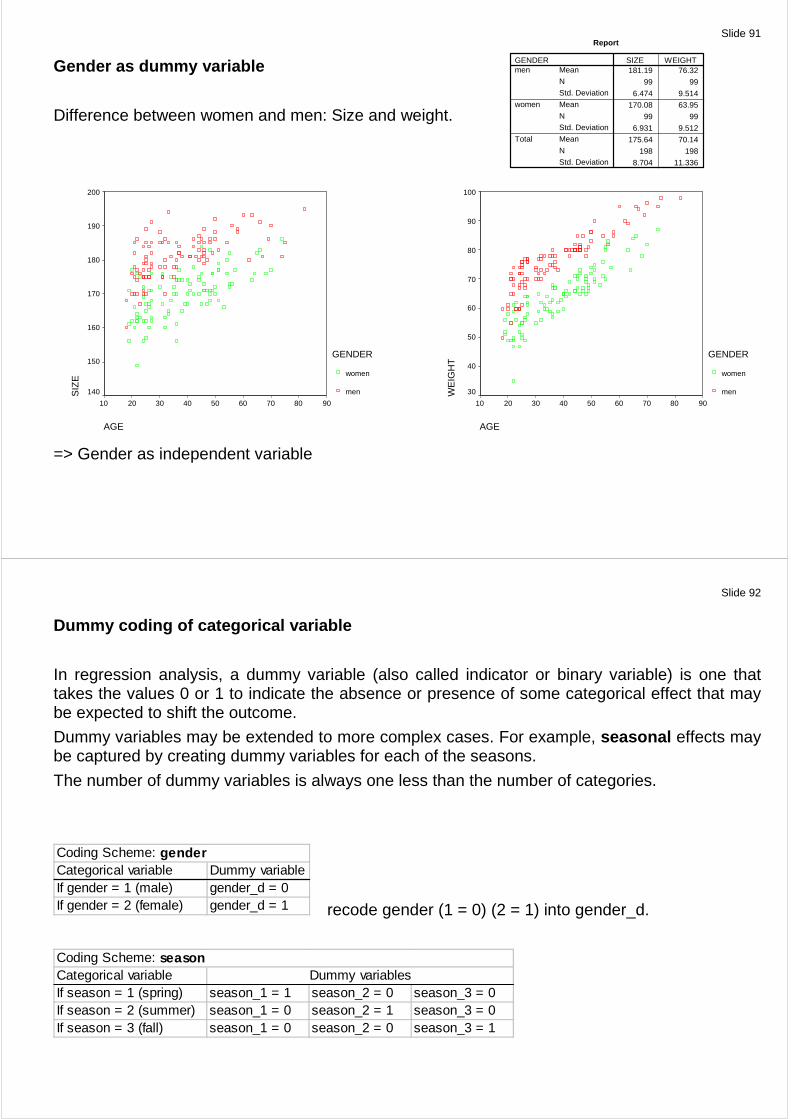
Gender as dummy variable
Difference between women and men: Size and weight.
AGE
908070605040302010
SIZ
E
200
190
180
170
160
150
140
GENDER
women
men
AGE
908070605040302010
WE
IGH
T
100
90
80
70
60
50
40
30
GENDER
women
men
=> Gender as independent variable
Report
181.19 76.32
99 99
6.474 9.514
170.08 63.95
99 99
6.931 9.512
175.64 70.14
198 198
8.704 11.336
Mean
N
Std. Deviation
Mean
N
Std. Deviation
Mean
N
Std. Deviation
GENDERmen
women
Total
SIZE WEIGHT
Slide 92
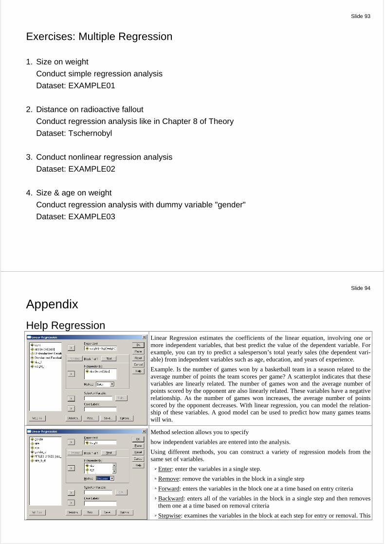
Dummy coding of categorical variable
In regression analysis, a dummy variable (also called indicator or binary variable) is one that takes the values 0 or 1 to indicate the absence or presence of some categorical effect that may be expected to shift the outcome.
Dummy variables may be extended to more complex cases. For example, seasonal effects may be captured by creating dummy variables for each of the seasons.
The number of dummy variables is always one less than the number of categories.
Categorical variable Dummy variableIf gender = 1 (male) gender_d = 0If gender = 2 (female) gender_d = 1
Coding Scheme: gender
recode gender (1 = 0) (2 = 1) into gender_d.
Categorical variableIf season = 1 (spring) season_1 = 1 season_2 = 0 season_3 = 0If season = 2 (summer) season_1 = 0 season_2 = 1 season_3 = 0If season = 3 (fall) season_1 = 0 season_2 = 0 season_3 = 1
Coding Scheme: seasonDummy variables
Slide 93
Exercises: Multiple Regression
1. Size on weight
Conduct simple regression analysis
Dataset: EXAMPLE01
2. Distance on radioactive fallout
Conduct regression analysis like in Chapter 8 of Theory
Dataset: Tschernobyl
3. Conduct nonlinear regression analysis
Dataset: EXAMPLE02
4. Size & age on weight
Conduct regression analysis with dummy variable "gender"
Dataset: EXAMPLE03
Slide 94
Appendix
Help Regression
Linear Regression estimates the coefficients of the linear equation, involving one or more independent variables, that best predict the value of the dependent variable. For example, you can try to predict a salesperson’s total yearly sales (the dependent vari-able) from independent variables such as age, education, and years of experience.
Example. Is the number of games won by a basketball team in a season related to the average number of points the team scores per game? A scatterplot indicates that these variables are linearly related. The number of games won and the average number of points scored by the opponent are also linearly related. These variables have a negative relationship. As the number of games won increases, the average number of points scored by the opponent decreases. With linear regression, you can model the relation-ship of these variables. A good model can be used to predict how many games teams will win.
Method selection allows you to specify
how independent variables are entered into the analysis.
Using different methods, you can construct a variety of regression models from the same set of variables. ◦ Enter: enter the variables in a single step. ◦ Remove: remove the variables in the block in a single step ◦ Forward: enters the variables in the block one at a time based on entry criteria ◦ Backward: enters all of the variables in the block in a single step and then removes
them one at a time based on removal criteria ◦ Stepwise: examines the variables in the block at each step for entry or removal. This
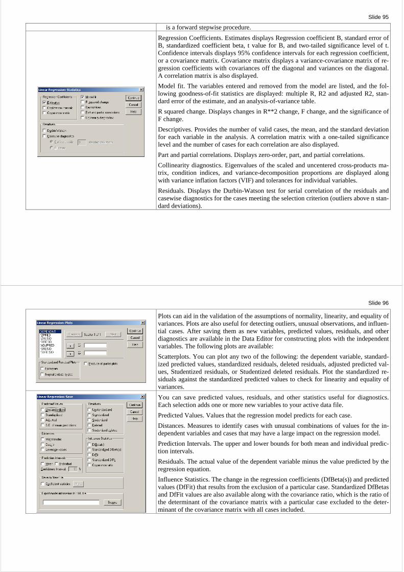
Slide 95
is a forward stepwise procedure.
Regression Coefficients. Estimates displays Regression coefficient B, standard error of B, standardized coefficient beta, t value for B, and two-tailed significance level of t. Confidence intervals displays 95% confidence intervals for each regression coefficient, or a covariance matrix. Covariance matrix displays a variance-covariance matrix of re-gression coefficients with covariances off the diagonal and variances on the diagonal. A correlation matrix is also displayed.
Model fit. The variables entered and removed from the model are listed, and the fol-lowing goodness-of-fit statistics are displayed: multiple R, R2 and adjusted R2, stan-dard error of the estimate, and an analysis-of-variance table.
R squared change. Displays changes in R**2 change, F change, and the significance of F change.
Descriptives. Provides the number of valid cases, the mean, and the standard deviation for each variable in the analysis. A correlation matrix with a one-tailed significance level and the number of cases for each correlation are also displayed.
Part and partial correlations. Displays zero-order, part, and partial correlations.
Collinearity diagnostics. Eigenvalues of the scaled and uncentered cross-products ma-trix, condition indices, and variance-decomposition proportions are displayed along with variance inflation factors (VIF) and tolerances for individual variables.
Residuals. Displays the Durbin-Watson test for serial correlation of the residuals and casewise diagnostics for the cases meeting the selection criterion (outliers above n stan-dard deviations).
Slide 96
Plots can aid in the validation of the assumptions of normality, linearity, and equality of variances. Plots are also useful for detecting outliers, unusual observations, and influen-tial cases. After saving them as new variables, predicted values, residuals, and other diagnostics are available in the Data Editor for constructing plots with the independent variables. The following plots are available:
Scatterplots. You can plot any two of the following: the dependent variable, standard-ized predicted values, standardized residuals, deleted residuals, adjusted predicted val-ues, Studentized residuals, or Studentized deleted residuals. Plot the standardized re-siduals against the standardized predicted values to check for linearity and equality of variances.
You can save predicted values, residuals, and other statistics useful for diagnostics. Each selection adds one or more new variables to your active data file.
Predicted Values. Values that the regression model predicts for each case.
Distances. Measures to identify cases with unusual combinations of values for the in-dependent variables and cases that may have a large impact on the regression model.
Prediction Intervals. The upper and lower bounds for both mean and individual predic-tion intervals.
Residuals. The actual value of the dependent variable minus the value predicted by the regression equation.
Influence Statistics. The change in the regression coefficients (DfBeta(s)) and predicted values (DfFit) that results from the exclusion of a particular case. Standardized DfBetas and DfFit values are also available along with the covariance ratio, which is the ratio of the determinant of the covariance matrix with a particular case excluded to the deter-minant of the covariance matrix with all cases included.