sprite lfs or let's log everything

Sprite LFSor Let's Log Everything

Robert GrimmNew York University

The Three Questions

What is the problem?

What is new or different?

What are the contributions and limitations?

MotivationTechnology

Processor speed is (still) increasing rapidly — or is it?

Main memory size is also increasing rapidly

But disk speeds (notably, access times) are not

Hence, we can cache a lot of data and writes dominate

Workloads

Office applications dominated by writes to small(ish) files

Existing file systems

Require many different writes to different locations

Do these writes synchronously, at least for metadata

Become a central bottleneck

Log-Structured File Systems

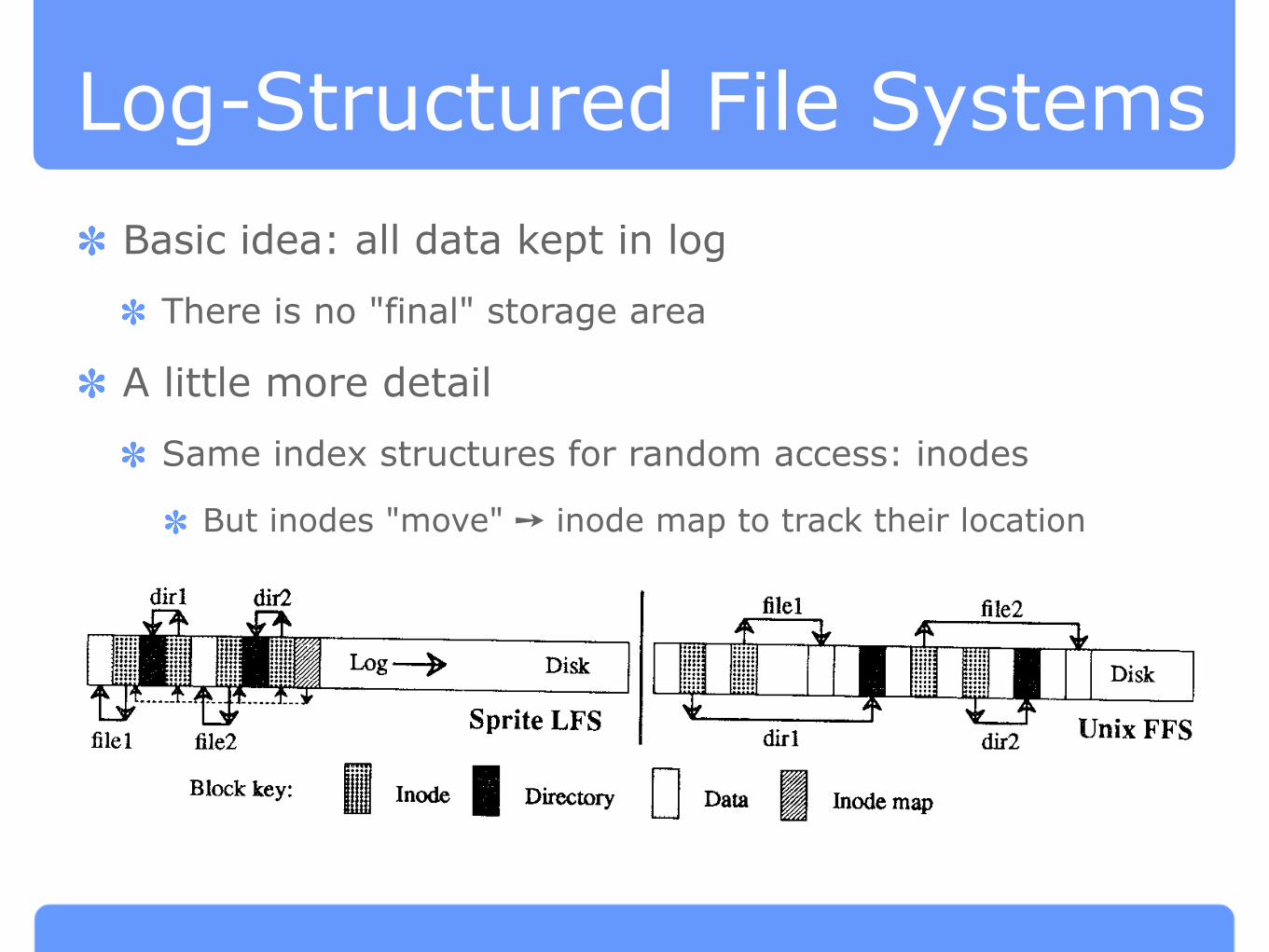
Basic idea: all data kept in log

There is no "final" storage area

A little more detail

Same index structures for random access: inodes

But inodes "move" ➙ inode map to track their location32 . M, Rosenblum and J. K. Ousterhout

dirl dir2 filel file2

‘1 &.* ~=Lag +

~ ........Disk &w

~: ;::;I ,, !!J~: ,,,, Disk,::: ~

Sprite LFS+ ‘?

filel file2 dirl dir2Unix FFS

Fig. 1. A comparison between Sprite LFS and Unix FFS. This example shows the modified disk

blocks written by Sprite LFS and Unix FFS when creating two single-block files named dirl /filel

and dlr2 /flle2. Each system must write new data blocks and inodes for file 1 and flle2, plus new

data blocks and inodes for the containing directories. Unix FFS requires ten nonsequential

writes for the new information (the inodes for the new files are each written twice to ease

recovery from crashes), while Sprite LFS performs the operations in a single large write. The

same number of disk accesses will be required to read the files in the two systems. Sprite LFS

also writes out new inode map blocks to record the new inode locations

Block Key:Threaded log

laOld log end New log end

Old datablock

New datablockII

Prcwously deletedII

Copy and Compact

Old log end New log end

Fig, 2. Possible free space management solutions for log-structured file systems, In a log-struc-

tured file system, free space for the log can be generated either by copying the old blocks or by

threading the log around the old blocks. The left side of the figure shows the threaded log

approach where the log skips over the active blocks and overwrites blocks of files that have beendeleted or overwritten. Pointers between the blocks of the log are mamtained so that the log can

be followed during crash recovery The right side of the figure shows the copying scheme where

log space is generated by reading the section of disk after the end of the log and rewriting the

active blocks of that section along with the new data into the newly generated space.

be no faster than traditional file systems. The second alternative is to copy

live data out of the log in order to leave large free extents for writing. For

this paper we will assume that the live data is written back in a compacted

form at the head of the log; it could also be moved to another log-structured

file system to form a hierarchy of logs, or it could be moved to some totally

different file system or archive. The disadvantage of copying is its cost,

particularly for long-lived files; in the simplest case where the log works

circularly across the disk and live data is copied back into the log, all of the

long-lived files will have to be copied in every pass of the log across the disk.

Sprite LFS uses a combination of threading and copying. The disk is

divided into large fixed-size extents called segments. Any given segment is

always written sequentially from its beginning to its end, and all live data

must be copied out of a segment before the segment can be rewritten.

However, the log is threaded on a segment-by-segment basis; if the system

ACM Transactions on Computer Systems, Vol. 10, No. 1, February 1992,

How to Manage Free Space?Goal: need large free disk regions for writing new data

Two solutions

Threading leaves data in place

But also leads fragmentation

Copying compacts data every so often

But also adds considerable overheads

LFS approach: do both

Threading at a large granularity ➙ segments

Need a table to track live segments: segment usage table

Copying at block granularity

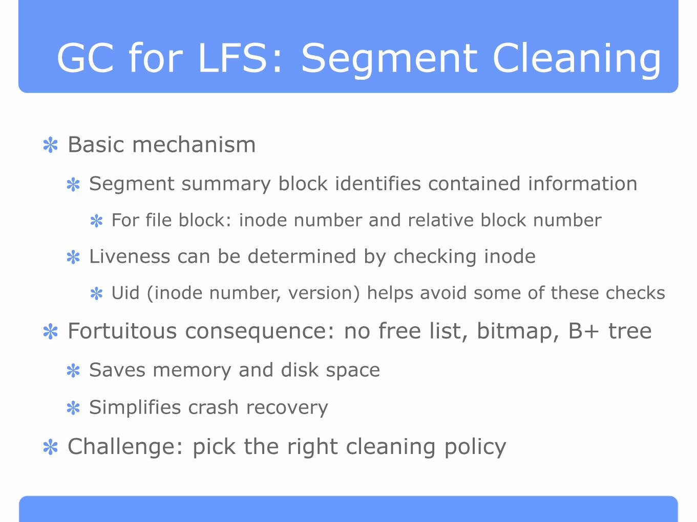
GC for LFS: Segment Cleaning

Basic mechanism

Segment summary block identifies contained information

For file block: inode number and relative block number

Liveness can be determined by checking inode

Uid (inode number, version) helps avoid some of these checks

Fortuitous consequence: no free list, bitmap, B+ tree

Saves memory and disk space

Simplifies crash recovery

Challenge: pick the right cleaning policy

Cleaning Policy Choices

When to clean?

Continuously, at night, when space is exhausted?

How many segments to clean?

More segments ➙ more opportunities for (re)arranging data

Which segments to clean?

Most fragmented ones?

How to group live blocks when cleaning?

By directory, by age?

Here: focus on latter, harder two questions

Simple thresholds used for when and how many

The Write Cost Metric

Intuition: avg. time disk is busy for writing new data

Including overhead of segment cleaning

Definition:

Large segments ➙ seek and rotational latency negligible

Remaining overhead: moving data to and from disk

Write cost expressed as multiplication factor

The Design and Implementation of a Log-Structured File System . 35

utilization (the fraction of data still live) in the segments that are cleaned. In

the steady state, the cleaner must generate one clean segment for every

segment of new data written. To do this, it reads N segments in their entirety

and writes out N* u segments of live data (where u is the utilization of the

segments and O < u < 1). This creates N*(1 – u) segments of contiguous free

space for new data. Thus

total bytes read and writtenwrite cost =

new data written

read segs + write live + write new—

new data written

N+ N*u+N*(l–u) 2— —— (1)

N*(l-zL) ‘I-u

In the above formula we made the conservative assumption that a segment

must be read in its entirety to recover the live blocks; in practice it may be

faster to read just the live blocks, particularly if the utilization is very low

(we haven’t tried this in Sprite LFS). If a segment to be cleaned has no live

blocks (u = O) then it need not be read at all and the write cost is 1.0.

Figure 3 graphs the write cost as a function of u. For reference, Unix FFS

on small file workloads utilizes at most 5 – 109ZO of the disk bandwidth, for a

write cost of 10–20 (see Ousterhout [16] and Figure 8 in Section 5.1 for

specific measurements). With logging, delayed writes, and disk request sort -

ing this can probably be improved to about 2590 of the bandwidth [24] or a

write cost of 4. Figure 3 suggests that the segments cleaned must have a

utilization of less than .8 in order for a log-structured file system to outper-

form the current Unix FFS; the utilization must be less than .5 to outperform

an improved Unix FFS.

It is important to note that the utilization discussed above is not the

overall fraction of the disk containing live data; it is just the fraction of live

blocks in segments that are cleaned. Variations in file usage will cause some

segments to be less utilized than others, and the cleaner can choose the least

utilized segments to clean; these will have lower utilization than the overall

average for the disk.

Even so, the performance of a log-structured file system can be improved by

reducing the overall utilization of the disk space. With less of the disk in use,

the segments that are cleaned will have fewer live blocks, resulting in a

lower write cost. Log-structured file systems provide a cost-performance

trade-off if disk space is underutilized, higher performance can be achieved

but at a high cost per usable byte; if disk capacity utilization is increased,

storage costs are reduced but so is performance. Such a trade-off between

performance and space utilization is not unique to log-structured file sys-

tems. For example, Unix FFS only allows 9070 of the disk space to be

occupied by files. The remaining 10’%o is kept free to allow the space alloca-

tion algorithm to operate efficiently.

ACM Transactions on Computer Systems, Vol. 10, No, 1, February 1992.

More on Write Cost

Utilization: live blocks in segments being cleaned

Not overall fraction of the disk containing live data

Key to high performance: bimodal segment distribution

Most segments nearly full

Few nearly empty segments (i.e., low utilization u)

Usually worked on by cleaner

Result: high overall utilization, low write cost

Trade off between disk utilization and performance

Typical of almost all file systems

Initial Simulation Results

Write 4KB files, greedily clean segments with lowest u

Uniform: all files equally likely to be written

Hot-and-cold: 10% of files get 90% of writes

Live blocks sorted by age during cleaning


Write cost

12.0 “-~{.----------”-: LFS hot-and-cold

&O --\

Go --~

0.0.. ; .. ... .. ..~.---.- ..-:.... .. .... . .. ... .. .. . .. .. ... ....

0.0 0.2 0.4 0.6 0:8 1:0

Disk capacity utilization

Fig. 4. Initial simulation results. The curves labeled “FFS today” and “FFS improved” are

reproduced from Figure 3 for comparison, The curve labeled “No variance” shows the write cost

that would occur if all segments always had exactly the same utilization. The “LFS uniform”

curve represents a log-structured file system with uniform access pattern and a greedy cleaning

policy: the cleaner chooses the least-utilized segments. The “LFS hot-and-cold” curve represents

a log-structured file system with locality of file access. It uses a greedy cleaning policy and the

cleaner also sorts the live data by age before writing it out again. The x-axis is overall disk

capacity utilization, which is not necessarily the same as the utilization of the segments being

cleaned.

In this approach the overall disk capacity utilization is constant and no read

traffic is modeled. The simulator runs until all clean segments are ex-

hausted, then simulates the actions of a cleaner until a threshold number of

clean segments is available again. In each run the simulator was allowed to

run until the write cost stabilized and all cold-start variance had been

removed.

Figure 4 superimposes the results from two sets of simulations onto the

curves of Figure 3. In the “LFS uniform” simulations the uniform access

pattern was used. The cleaner used a simple greedy policy where it always

chose the least-utilized segments to clean. When writing out live data the

cleaner did not attempt to reorganize the data: live blocks were written out in

the same order that they appeared in the segments being cleaned (for a

uniform access pattern there is no reason to expect any improvement from

reorganization).

Even with uniform random access patterns, the variance in segment uti-

lization allows a substantially lower write cost than would be predicted from

the overall disk capacity utilization and formula (1). For example, at 75%

overall disk capacity utilization, the segments cleaned have an average

utilization of only 55%. At overall disk capacity utilization under 2090 the

write cost drops below 2.0; this means that some of the cleaned segments

have no live blocks at all and hence don’t need to be read in.

The “LFS hot-and-cold” curve shows the write cost when there is locality in

the access patterns, as described above. The cleaning policy for this curve

was the same as for “LFS uniform” except that the live blocks were sorted by

ACM Transactions on Computer Systems, Vol. 10, No. 1, February 1992.

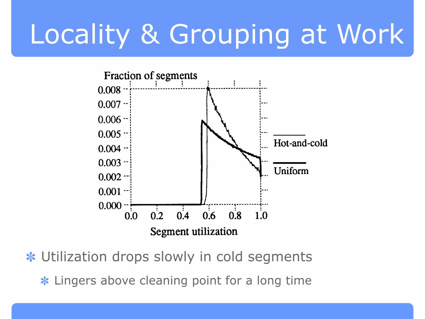
Locality & Grouping at Work

Utilization drops slowly in cold segments

Lingers above cleaning point for a long time


Fraction of segments

~.~g .. ;..... ....!--!-....

0.007 ‘- I

f).f)~ --~\

().005 --~

0.004 ‘-;

0.003 ‘-~

0.002 --~

(),001 --~ ;...

O.000 --~ ...........,---.----+.

0.0 0:2 0:4 0:6 0:8 1.0

Segment utilization

Fig. 5. Segment utilization distributions with greedy cleaner. These figures show distributions

of segment utilizations of the disk during the simulation. The distribution is computed by

measuring the utilizations of all segments on the disk at the points during the simulation when

segment cleaning was initiated. The distribution shows the utilizations of the segments avail-

able to the cleaning algorithm. Each of the distributions corresponds to an overall disk capacity

utilization of 75Y0. The “Uniform” curve Corresponds to ‘ ‘LFS uniform” in F@re 4 and

“H&aml-colcl” corresponds to “LFS hot-and-cold” in Figure 4. Locality causes the distribution to

be more skewed towards the utilization at which cleaning occurs; as a result, segments are

cleaned at a higher average utilization.

Fraction of segmentso.m8 ..L ........L...L......

0.007 -“j

0.006 -j

0.005 --+

0.004 --j

0.003 --j.. LFS Cost-Benefit

0.002 --~

().001 --j

0.000 --:4 L.. . . . . . . . . . . . . . . . . . .!. .

0.0 0:2 0:4 0:6 0:8 1.0

Segment utilization

Fig. 6. Segment utilization distribution with cost-benefit policy. This figure shows the distribu-

tion of segment utilizations from the simulation of a hot-and-cold access pattern with 75% overall

disk capacity utilization. The “LFS Cost-Benefit” curve shows the segment distribution occur-

ring when the cost-benefit policy is used to select segments to clean and live blocks are grouped

by age before being rewritten. Because of this bimodal segment distribution, most of the

segments cleaned had utilizations around 15!%. For comparison, the distribution produced by the

greedy method selection policy is shown by the “LFS Greedy” curve reproduced from Figure 5.

ACM TransactIons on Computer Systems, Vol. 10, No. 1, February 1992

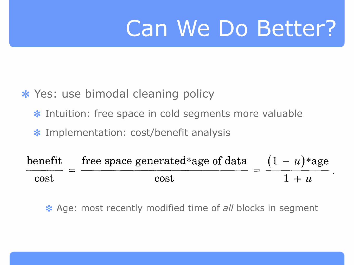
Can We Do Better?

Yes: use bimodal cleaning policy

Intuition: free space in cold segments more valuable

Implementation: cost/benefit analysis

Age: most recently modified time of all blocks in segment

38 . M, Rosenblum and J, K. Ousterhout

age before writing them out again. This means that long-lived (cold) data

tends to be segregated in different segments from short-lived (hot) data; we

thought that this approach would lead to the desired bimodal distribution of

segment utilizations.

Figure 4 shows the surprising result that locality and “better” grouping

result in worse performance than a system with no locality! We tried varying

the degree of locality (e.g., 95% of accesses to 5% of data) and found that

performance got worse and worse as the locality increased. Figure 5 shows

the reason for this nonintuitive result. Under the greedy policy, a segment

doesn’t get cleaned until it becomes the least utilized of all segments. Thus

every segment’s utilization eventually drops to the cleaning threshold, in-

cluding the cold segments. Unfortunately, the utilization drops very slowly in

cold segments, so these segments tend to linger just above the cleaning point

for a very long time. Figure 5 shows that many more segments are clustered

around the cleaning point in the simulations with locality than in the

simulations without locality. The overall result is that cold segments tend to

tie up large numbers of free blocks for long periods of time.

After studying these figures we realized that hot and cold segments must

be treated differently by the cleaner. Free space in a cold segment is more

valuable than free space in a hot segment because once a cold segment has

been cleaned it will take a long time before it reaccumulates the unusable

free space. Said another way, once the system reclaims the free blocks from a

segment with cold data it will get to “keep” them a long time before the cold

data becomes fragmented and “takes them back again. ” In contrast, it is less

beneficial to clean a hot segment because the data will likely die quickly and

the free space will rapidly reaccumulate; the system might as well delay the

cleaning a while and let more of the blocks die in the current segment. The

value of a segment’s free space is based on the stability of the data in the

segment. Unfortunately, the stability cannot be predicted without knowing

future access patterns. Using an assumption that the older the data in a

segment the longer it is likely to remain unchanged, the stability can be

estimated by the age of data.

To test this theory we simulated a new policy for selecting segments to

clean. The policy rates each segment according to the benefit of cleaning the

segment and the cost of cleaning the segment and chooses the segments with

the highest ratio of benefit to cost. The benefit has two components: the

amount of free space that will be reclaimed and the amount of time the space

is likely to stay free. The amount of free space is just 1 – u, where u is the

utilization of the segment. We used the most recent modified time of any

block in the segment (i.e., the age of the youngest block) as an estimate of

how long the space is likely to stay free. The benefit of cleaning is the

space-time product formed by multiplying these two components. The cost of

cleaning the segment is 1 + u (one unit of cost to read the segment, u to

write back the live data). Combining all these factors, we get

benefit free space generated* age of data (1 - u)*age— ——

cost – cost l+U “


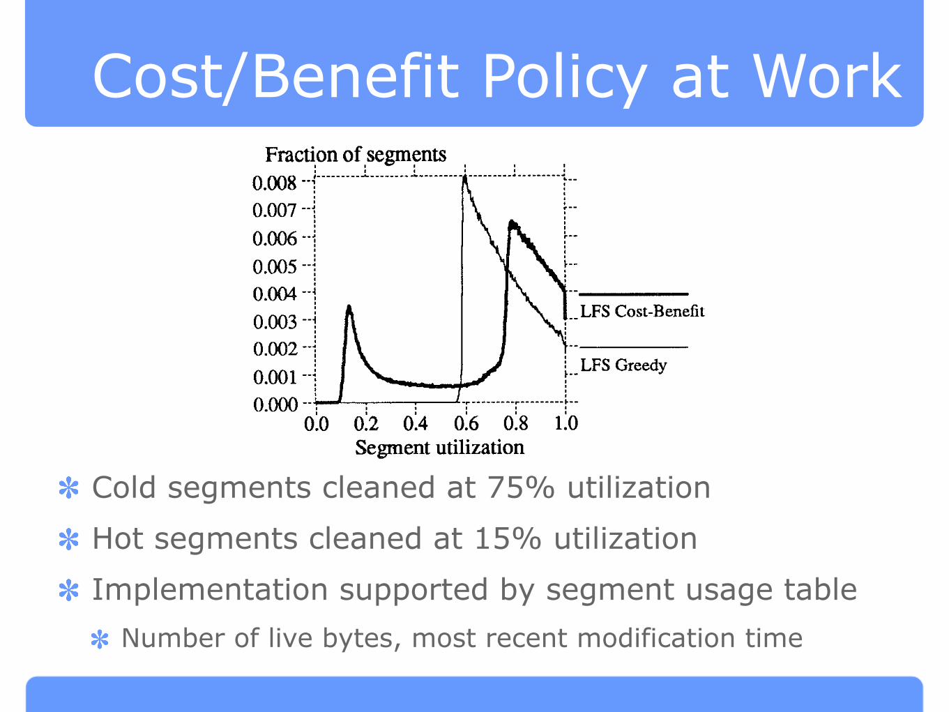
Cost/Benefit Policy at Work

Cold segments cleaned at 75% utilization

Hot segments cleaned at 15% utilization

Implementation supported by segment usage table

Number of live bytes, most recent modification time



~.~g .. ;..... ....!--!-....

0.007 ‘- I

f).f)~ --~\

().005 --~

0.004 ‘-;

0.003 ‘-~

0.002 --~

(),001 --~ ;...

O.000 --~ ...........,---.----+.

0.0 0:2 0:4 0:6 0:8 1.0

Segment utilization

Fig. 5. Segment utilization distributions with greedy cleaner. These figures show distributions

of segment utilizations of the disk during the simulation. The distribution is computed by

measuring the utilizations of all segments on the disk at the points during the simulation when

segment cleaning was initiated. The distribution shows the utilizations of the segments avail-

able to the cleaning algorithm. Each of the distributions corresponds to an overall disk capacity

utilization of 75Y0. The “Uniform” curve Corresponds to ‘ ‘LFS uniform” in F@re 4 and

“H&aml-colcl” corresponds to “LFS hot-and-cold” in Figure 4. Locality causes the distribution to

be more skewed towards the utilization at which cleaning occurs; as a result, segments are

cleaned at a higher average utilization.

Fraction of segmentso.m8 ..L ........L...L......

0.007 -“j

0.006 -j

0.005 --+

0.004 --j

0.003 --j.. LFS Cost-Benefit

0.002 --~

().001 --j

0.000 --:4 L.. . . . . . . . . . . . . . . . . . .!. .

0.0 0:2 0:4 0:6 0:8 1.0

Segment utilization

Fig. 6. Segment utilization distribution with cost-benefit policy. This figure shows the distribu-

tion of segment utilizations from the simulation of a hot-and-cold access pattern with 75% overall

disk capacity utilization. The “LFS Cost-Benefit” curve shows the segment distribution occur-

ring when the cost-benefit policy is used to select segments to clean and live blocks are grouped

by age before being rewritten. Because of this bimodal segment distribution, most of the

segments cleaned had utilizations around 15!%. For comparison, the distribution produced by the

greedy method selection policy is shown by the “LFS Greedy” curve reproduced from Figure 5.


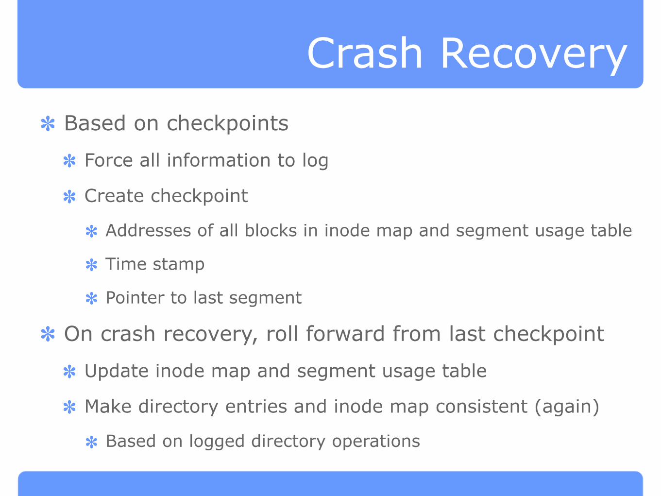
Crash Recovery

Based on checkpoints

Force all information to log

Create checkpoint

Addresses of all blocks in inode map and segment usage table

Time stamp

Pointer to last segment

On crash recovery, roll forward from last checkpoint

Update inode map and segment usage table

Make directory entries and inode map consistent (again)

Based on logged directory operations

Evaluation

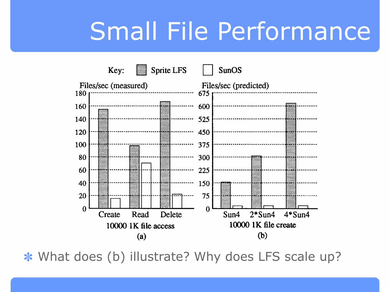
Small File Performance

What does (b) illustrate? Why does LFS scale up?


Key: ! SpriteLFS ! SunOS

Files/see (measured)180 [--------------------------------------------------

160

140

120

100

80

60

40

20

0

10000 lK file access

(a)

Files/see (predicted)675 [--------------------------------------------------

600

525

450

375

300

225

150

75

0

I r

. . . . . . . . . . . . . . . . . . . . . . . . . . . . . . . . . . . . . . . . .

. . . . . . . . . .---------- . . . . . . . . . . . . . .

I....................................................................I

y ‘--

1111............-....-.-.........-

10000 lK file create

m)

Fig. 8. Small-file performance under Sprite LFS and SunOS. (a) measures a benchmark that

created 10000 one-kilobyte files, then read them back in the same order as created, then deleted

them. Speed is measured by the number of files per second for each operation on the two file

systems. The logging approach in Sprite LFS provides an order-of-magnitude speedup for

creation and deletion. (h) estimates the performance of each system for creating files on faster

computers with the same disk. In SunOS the disk was 8570 saturated in (a), so faster processors

will not improve performance much. In Sprite LFS the disk was only 17% saturated in (a) while

the CPU was 100% utilized; as a consequence 1/0 performance will scale with CPU speed,

optimally on disk for the assumed read patterns. In contrast, a log-structured

file system achieves temporal locality: information that is created or modified

at the same time will be grouped closely on disk. If temporal locality matches

logical locality, as it does for a file that is written sequentially and then read

sequentially, then a log-structured file system should have about the same

performance on large files as a traditional file system. If temporal locality

differs from logical locality then the systems will perform differently. Sprite

LFS handles random writes more efficiently because it writes them sequen-

tially on disk. SunOS pays more for the random writes in order to achieve

logical locality, but then it handles sequential rereads more efficiently.

Random reads have about the same performance in the two systems, even

though the blocks are laid out very differently. However, if the nonsequential

reads occurred in the same order as the nonsequential writes then Sprite

would have been much faster.

5.2 Cleaning Overheads

The micro-benchmark results of the previous section give an optimistic view

of the performance of Sprite LFS because they do not include any cleaning

overheads (the write cost during the benchmark runs was 1. O). In order to

ACM Transactions on Computer Systems, Vol. 10, No. 1, February 1992.

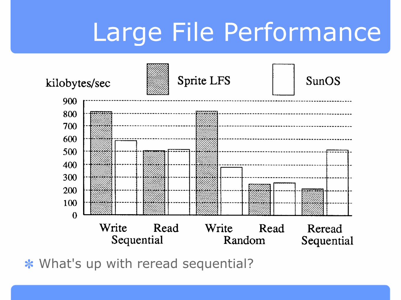
Large File Performance

What's up with reread sequential?

46 . M. Rosenblum and J K. Ousterhout

kilobytes/see Sprite LFS

El

SunOS

900 [-----""--"---"-""----"--"---------------------"""--""""-------------------"-----------------------------

800

700

600

500

400

300

200

100

0

1--------------"----"-"--""-"----'-m--------------------""--"---------------------------

Write Read Write Read Reread

Sequential Random Sequential

Fig. 9. Large-file performance under Sprite LFS and SunOS. The figure shows the speed of a

benchmark that creates a 100-Mbyte file with sequential writes, then reads the file back

sequentially, then writes 100 Mbytes randomly to the existing file, then reads 100 Mbytes

randomly from the file, and finally reads the file sequentially again, The bandwidth of each of

the five phases is shown separately, Sprite LFS has a higher write bandwidth and the same read

bandwidth as SunOS with the exception of sequential reading of a file that was written

randomly.

assess the cost of cleaning and the effectiveness of the cost-benefit cleaning

policy, we recorded statistics about our production log-structured file systems

over a period of several months. Five systems were measured:

/user6 Home directories for Sprite developers. Workload consists of

program development, text processing, electronic communica-

tion and simulations.

Ipcs Home directories and project area for research on parallel

processing and VLSI circuit design.

/src / kernel Sources and binaries for the Sprite kernel.

/swap2 Sprite client workstation swap files. Workload consists of

virtual memory backing store for 40 diskless Sprite workst a -

tions. Files tend to be large, sparse and accessed consequen-

tially.

Itmp Temporary file storage area for 40 Sprite workstations.

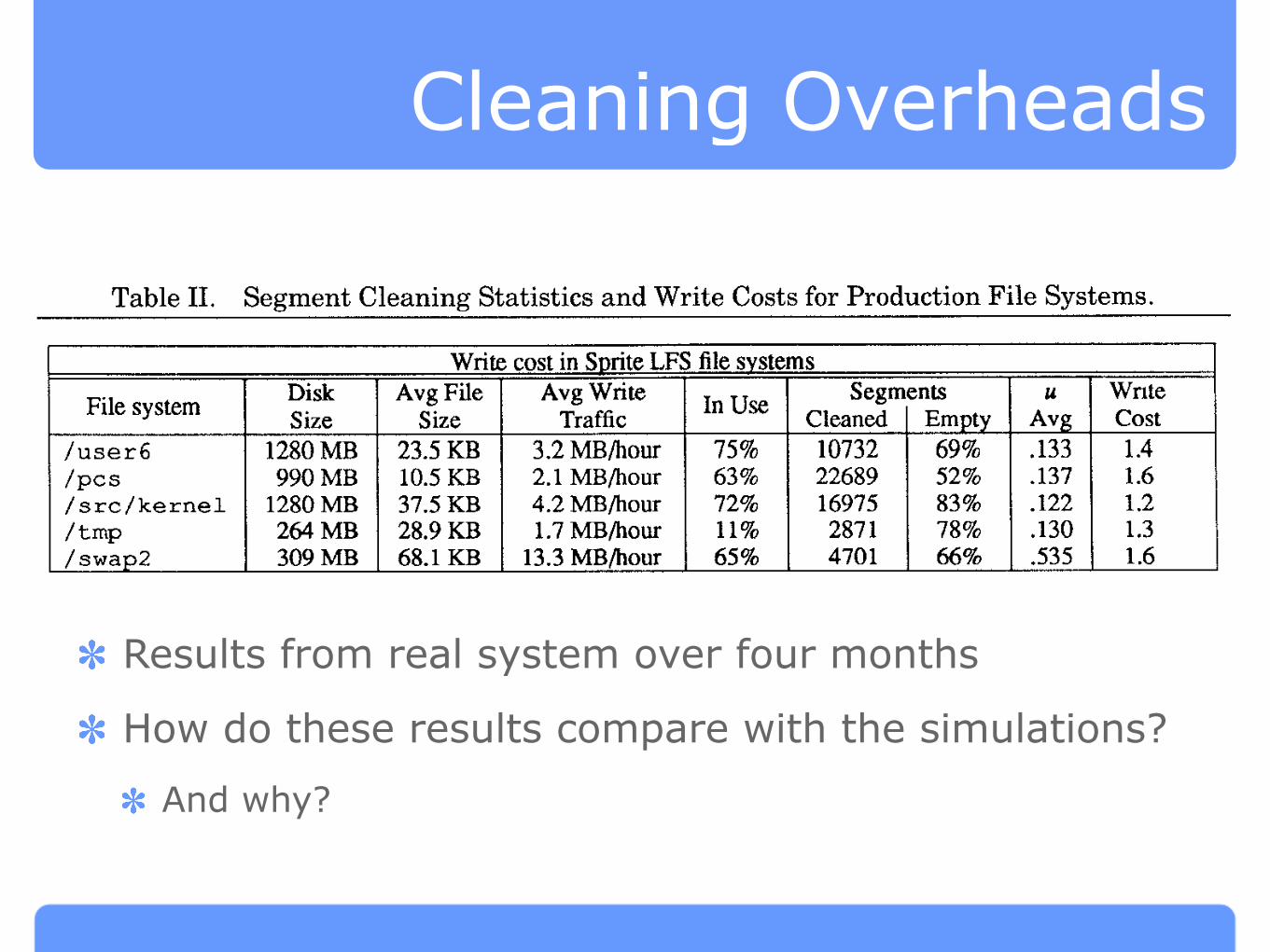
Table II shows statistics gathered during cleaning over a four-month

period. In order to eliminate start-up effects, we waited several months after

putting the file systems into use before beginning the measurements. The

behavior of the production file systems has been substantially better than

predicted by the simulations in Section 3. Even though the overall disk

capacity utilizations ranged from 11 – ‘75Y0, more than half of the segments

cleaned were totally empty. Even the nonempty segments have utilizations

far less than the average disk utilizations. The overall write costs ranged

ACM Transactions on Computer Systems, Vol 10, No 1, February 1992

Cleaning Overheads

Results from real system over four months

How do these results compare with the simulations?

And why?


Table II. Segment Cleaning Statistics and Write Costs for Production File Systems.

I File system I ::

Write cost in Smite LFS file systems—..

Avg File Avg WriteIn Use

Segments Write

~i7~ Traffic Cleaned Empty Atg cost

<B 3.2 MB/hoor 75% 10732 69% .133 1.452% .137 1.6

1 /sw;p2 309 MB 68.1 KB 13.3 MB/hour 65% 4701 66% .535 1.6

For each Sprite LFS file system the table lists the disk size, the average file size, the average

daily write traffic rate, the average disk capacity utilization, the total number of segments

cleaned over a four-month period, the fraction of the segments that were empty when cleaned,

theaverage utilization of thenonempty segments that were cleaned, and the overall write cost

fortheperiod of the measurements. These write cost figures imply that the cleaning overhead

limits the long-term write performance to about 70% of the maximum sequential write band-

width.


0.180 --

0.160 ---

0.140 ‘-”

0.120 ‘-”

0.100 ‘-”

0.080 ‘-

0.060 --

0.040 ‘-”

.~.............{..............+.............+............. ...~

0.020 ““”~(jm -. ~-.~1 ... ............................................................

0.0 0:2 0:4 0:6 0:8 1:0

Segment utilization

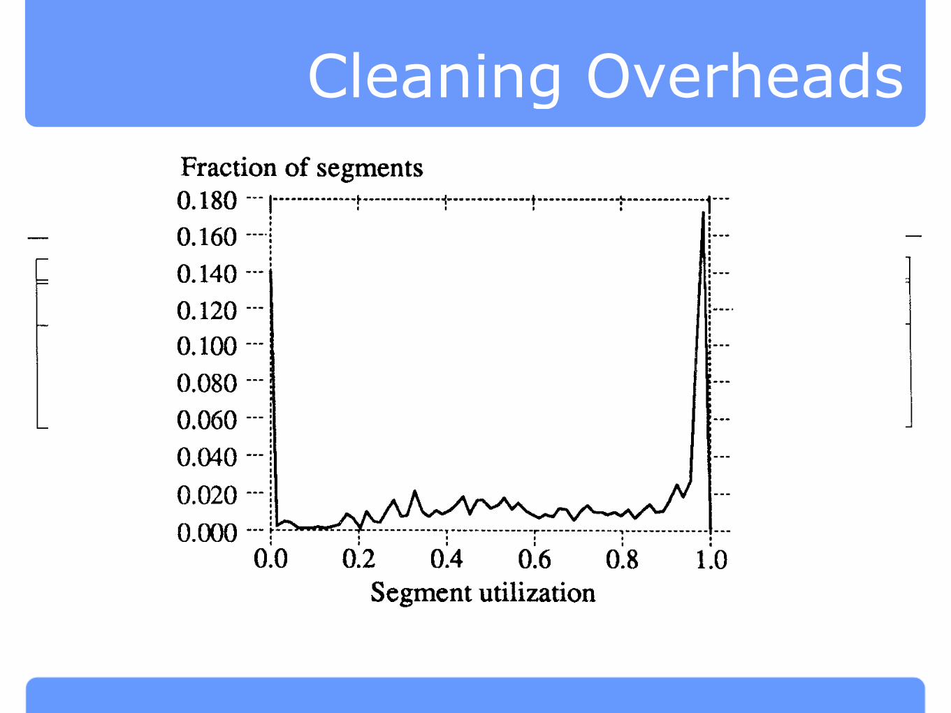
Fig. 10. Segment utilization in the /user6 tile system. This figure shows the distribution of

segment utilizations in a recent snapshot of the /user6 disk. The distribution shows large

numbers of fully utilized segments and totally empty segments.

from 1.2 to 1.6, in comparison to write costs of 2.5-3 in the corresponding

simulations. Figure 10 shows the distribution of segment utilizations,

gathered in a recent snapshot of the /user6 disk.

We believe that there are two reasons why cleaning costs are lower in

Sprite LFS than in the simulations. First, all the files in the simulations

were just a single block long. In practice, there are a substantial number of

longer files, and they tend to be written and deleted as a whole. This results

in greater locality within individual segments. In the best case where a file is

much longer than a segment, deleting the file will produce one or more

totally empty segments. The second difference between simulation and real-

ity is that the simulated reference patterns were evenly distributed within

ACM Transactions on Computer Systems, Vol. 10, No. 1, February 1992

Cleaning Overheads

Results from real system over four months

How do these results compare with the simulations?

And why?



I File system I ::



Segments Write


<B 3.2 MB/hoor 75% 10732 69% .133 1.452% .137 1.6

1 /sw;p2 309 MB 68.1 KB 13.3 MB/hour 65% 4701 66% .535 1.6







width.


0.180 --

0.160 ---

0.140 ‘-”

0.120 ‘-”

0.100 ‘-”

0.080 ‘-

0.060 --

0.040 ‘-”

.~.............{..............+.............+............. ...~

0.020 ““”~(jm -. ~-.~1 ... ............................................................

0.0 0:2 0:4 0:6 0:8 1:0

Segment utilization


















I File system I ::



Segments Write


<B 3.2 MB/hoor 75% 10732 69% .133 1.452% .137 1.6

1 /sw;p2 309 MB 68.1 KB 13.3 MB/hour 65% 4701 66% .535 1.6







width.


0.180 --

0.160 ---

0.140 ‘-”

0.120 ‘-”

0.100 ‘-”

0.080 ‘-

0.060 --

0.040 ‘-”

.~.............{..............+.............+............. ...~

0.020 ““”~(jm -. ~-.~1 ... ............................................................

0.0 0:2 0:4 0:6 0:8 1:0

Segment utilization
















What Do You Think?

sprite lfs or let's log everything

Documents