springfield,va22150 causes of microslip in a...
TRANSCRIPT

1
gtamnhtvac
d�Cc
rrn
uptnC
cicbcr
p22nb
J
Songho KimRaytheon UTD,
8350 Alban Road,Springfield, VA 22150
e-mail: [email protected]
Carl MooreDepartment of Mechanical Engineering,
Florida A&M University,Tallahassee, FL 32310
e-mail: [email protected]
Michael Peshkine-mail: [email protected]
J. Edward Colgatee-mail: [email protected]
Department of Mechanical Engineering,Northwestern University,
Evanston, IL 60208
Causes of Microslip in aContinuously VariableTransmissionThe continuously variable transmission (CVT) is a type of transmission that can adoptany arbitrary gear ratio. Whereas typical transmissions utilize toothed gears, the CVTemploys a sphere in rolling contact with a set of rollers; loads applied to the CVT aresupported across these rolling contacts, resulting in microslips of varying amounts ateach contact area. In this paper, we describe the causes of microslips in the CVT andways to lessen them through an alternative CVT design. �DOI: 10.1115/1.2803711�
IntroductionWhereas typical transmissions that utilize combinations of
ears can only adopt a fixed number of discrete transmission ra-ios, a continuously variable transmission, or simply CVT, candopt any arbitrary gear ratio between a minimum and a maxi-um. There exist numerous CVT designs and applications: Engi-
eers in the automotive industry, concerned with fuel efficiency,ave developed CVTs for use in powertrains. In this application,he CVT ratio can be adjusted to match any engine speed to anyehicle speed. Hence with vehicles that employ CVTs, engineersre able to design controllers to maximize engine power to fuelonsumption.
In the field of robotics, researchers at Northwestern Universityeveloped CVTs for use in human-machine devices, called cobotsshort for collaborative robots� �1�. In the framework of a cobot,VTs function as constraint mechanisms that place kinematiconstraints on the cobot’s joints.
1.1 Background. Most CVT only allow positive transmissionatios, but some can adopt both positive and negative transmissionatios; these latter transmissions are commonly known as infi-itely variable transmissions, or simply IVTs.
The CVT, which is the focus of this paper, used in cobots isnique in that it can adopt any transmission ratio, including bothositive and negative �. We may thus classify this particularransmission as an IVT; however, we will use the name and acro-ym given for this transmission in Ref. �2� and refer to it as theVT.CVTs are elemental in the design of a cobot. CVTs function as
onstraint mechanisms that are responsible for setting and enforc-ng the kinematic relationship of the cobot’s joints. In the Armobot �3� for example, three CVTs set the kinematic relationshipetween the Arm’s three rotational joints �Fig. 1�. Servomotors,onnected to each CVT, allow us to control the CVT settings ineal time, thereby allowing us to control the Arm’s end effector.
Contributed by the Power Transmission and Gearing Committee of ASME forublication in the JOURNAL OF MECHANICAL DESIGN. Manuscript received September 2,006; final manuscript received February 19, 2007; published online December 7,007. Review conducted by Teik C. Lim. Paper presented at the 2003 ASME Inter-ational Mechanical Engineering Congress �IMECE2003�, Washington, DC, Novem-
er 15–21, 2003.ournal of Mechanical Design Copyright © 20
The design of the CVT utilizes a sphere that is surrounded andheld in place by four rollers. Two of the four rollers, called steer-ing rollers, constrain the sphere to rotate about an axis of rotation,whose direction can be changed by adjusting the orientations ofthe steering rollers. The relative velocities of the remaining tworollers, called drive rollers, are dependent on the orientation of thesphere’s axis of rotation.
1.2 Motivation. The motivation for our analysis of the CVTstemmed from our physical interaction with existing cobots. Weobserved from our analysis of the cobots that the measured veloc-ity ratios of a pair of joints, connected by CVTs, differed notice-ably from the intended velocity ratios.
Ideally, the ratio of the angular velocities of a pair of roboticjoints, connected by CVTs, is the same as the transmission ratiosof the CVTs. In practice, however, the actual velocity ratio oftendeviates from the intended ratio. One contributor to this is mi-croslip �or creep� across the rolling contacts between the CVTsphere and the rollers; a force on a robot’s end point producestractive forces across the rolling contacts, thereby giving rise tomicroslip �or creep� at these rolling contacts.
Herein, we develop a model of the CVT microslip, verify themodel with experiments, and then use the model to simulate aproposed improvement to the CVT design.
1.3 Related Work. Akehurst et al. �4� give a good overviewof published works related to CVTs that operate through rollingtraction. Previous works concerning microslips in CVTs, utilizedin cobots, are limited. They include the kinematic creep model �5�of Gillespie et al. and the experimental analysis �6� of Brokowskiet al. of the CVT.
In Ref. �5�, Gillespie et al. model the drive rollers as rigidbodies that make line contacts with the sphere. They describe thatthe drive rollers transmit longitudinal forces across the rollingcontacts while under a state of spin.1 In their work, Gillespie et al.determine an expression for the velocity ratio as a function of thetransmission angle, load, and spin. The work of Gillespie et al. islimited to the analysis of slips at contacts between the sphere andthe drive rollers; their work does not examine the causes andeffects of slips at the contacts between the sphere and the steering
1
Spin refers to relative angular motion of the normal of two bodies in contact.JANUARY 2008, Vol. 130 / 011010-108 by ASME

r
CkBtao
ataadg
ScpS
2
dscTdo
dv
Fti
Fpr
0
ollers.The work of Brokowski et al. involves subjecting a physical
VT to experimental testing and comparing their results to theinematic creep model of Gillespie et al. In their work,rowkowski et al. thoroughly examine the mechanics of the con-
acts between the sphere and the drive rollers, but like Gillespie etl., Browkowski et al. also neglect to examine causes and effectsf slips of the contacts between the sphere and the steering rollers.
1.4 Preview of Sections. Our work concerns an experimentals well as an analytical analysis of the CVT. Through experimen-al analysis, we develop a kinetic model that describes the CVT’sbility to produce the desired velocity ratios in the face of loadscross the device. In addition, we develop an analytical model thatescribes the causes of microslips in the CVT and we offer sug-estions for the design of an improved CVT.
In Sec. 2, we describe the design and kinematics of the CVT. Inec. 3, we present an analytical model that describes the mi-roslips in the CVT. In Sec. 4, we verify our model through ex-eriments on a CVT that is subject to various loads. Finally, inec. 5, we describe the suggested designs of an improved CVT.
Continuously Variable Transmission
2.1 Continuously Variable Transmission Kinematics. Theesign of the CVT utilizes four rollers in rolling contact with aphere �Fig. 2�. Two of these rollers, called the steering rollers,onstrain the sphere to rotate about a particular axis of rotation.he relative motions between the remaining two rollers, called therive rollers, are dependent on the orientation of the sphere’s axisf rotation.
In Fig. 3, the three-dimensional coordinate frame N, with coor-inate axes x, y, and z, is fixed to the base of the CVT. The unitectors d1, d2, and d3 are established by rotating the coordinate
ig. 1 Structure of the Arm cobot. The motions of the cobot’shree rotational joints J1, J2, and J3 are related to the cobot’snternal motion as they are connected by three CVTs.
ig. 2 A CAD model of the CVT. The design of the CVT em-loys a sphere in rolling contact with four rollers „two drive
ollers and two steering rollers….11010-2 / Vol. 130, JANUARY 2008
frame N about the z-coordinate axis by 45 deg. The three orthogo-nal unit vectors ci�i=1,2 ,3� are established by rotating the frameN about the x-coordinate axis by 135 deg. The unit vector c3 is inthe positive x-coordinate direction. The unit vectors c1 and c2 aredefined using the right-hand rule. The center of the sphere O islocated at the origin of the coordinate frame N.
Figure 3�a� shows the drive Rollers D1 and D2. The center ofthe contact patch between the sphere O and the Roller D1 lies onan axis that is collinear to the unit vector d2. Drive Roller D1 hasan angular velocity �1 about an axis that is parallel to the unitvector d1. The center of the contact patch between O and D2 lieson an axis that is collinear to the unit vector d1. Drive Roller D2has an angular velocity �2 about an axis that is parallel to thevector d2.
Figure 3�b� shows the steering Rollers S1 and S2 and the steer-ing Forks C1 and C2. C1 rotates about an axis that is collinear tothe unit vector c1. The center of the contact patch between thesphere O and the Roller S1 lies on an axis that is collinear to theunit vector c1. C2 rotates about an axis that is collinear to the unitvector c2. The center of the contact patch between O and theRoller S2 lies on an axis that is collinear to the unit vector c2. C1and C2 are mechanically coupled via a bevel gear �not shown�such that the orientations of C1 and C2 can be described by thesame steering angle �. The coordinate axis s1 is fixed to C1 andthe coordinate axis s2 is fixed to C2. Steering Roller S1 has anangular velocity �S about s1 and steering Roller S2 has an angularvelocity �S about s2.
Figure 4�a� shows the sphere O and steering Roller S1; steeringRoller S2 and the two drive rollers are not shown. Figure 4�b�shows the sphere and the steering Roller S2; steering Roller S1and the two drive rollers are not shown. Let r be the radius of thesteering rollers and let R be the radius of the sphere O. Then, therolling constraint between the Roller S1 and O, whose velocity is�, requires that
� � Rc1 = ��S cos �c2 + �S sin �c3� � �− rc1� �1�
Also, the rolling constraint between the Roller S2 and O requiresthat
� � Rc2 = ��S cos �c1 + �S sin �c3� � �− rc2� �2�
Fig. 3 The design of the CVT includes a sphere and four roll-ers. In „a…, only the drive rollers are shown and in „b…, only thesteering rollers are shown.
Combining Eqs. �1� and �2�, we have
Transactions of the ASME

O
Wad
aur
tr
AO
Eb
Fb
Fs
J
� =r�S
R�− cos �c1 − cos �c2 − sin �c3� �3�
r we may write
� =r�S
R��2 cos � − sin �
�2d1 +
�2 cos � + sin �
�2d2� �4�
e see that from the above equation, the sphere’s instantaneousxis of rotation lies on a plane defined by the unit vectors d1 and2.Let t be an axis that is collinear to the sphere’s instantaneous
xis of rotation �Fig. 5� and let � describe the angle between thenit vector d1 and the axis t. Then, �, called the CVT angle, iselated to the steering angle � by
� = tan−1��2 + tan �
�2 − tan �� �5�
Let �O be the sphere’s angular velocity about the axis t. Then,he rolling constraint between the Roller D1 and the sphere Oequires that
− �1d1 � − rd2 = ��O cos �d1 + �O sin �d2� � Rd2 �6�lso, the rolling constraint between the Roller D2 and the sphererequires that
− �2d2 � − rd1 = ��O cos �d1 + �O sin �d2� � Rd1 �7�quations �6� and �7� can be combined to find the relationshipetween the velocities of the drive rollers and the CVT angle �:
ig. 4 Two additional views of the CVT. The orientations ofoth steering rollers are described by steering angle �.
ig. 5 The sphere’s instantaneous axis of rotation is de-
cribed by the CVT angle �ournal of Mechanical Design
�2
�1= tan � �8�
Equation �8� is called the ideal transmission law. We may com-bine Eqs. �5� and �8� to find an alternative expression of the idealtransmission law:
�2
�1=
�2 + tan �
�2 − tan ��9�
2.1.1 Continuously Variable Transmission Velocity Vector. Wecan express the velocities of both drive rollers as a vector in atwo-dimensional Cartesian coordinate system �Fig. 6�. The two-dimensional Cartesian coordinate system V has unit vectors v1 andv2 in the positive directions of the x- and y-coordinate axes, re-spectively. A point in the coordinate space V represents the dis-placements of drive Rollers D1 and D2; the x component repre-sents the displacement of D1 and the y component represents thedisplacement of D2. A vector that locates this point represents thevelocities of both drive rollers. The two-dimensional Cartesiancoordinate system U is established by rotating coordinate systemV about an axis that passes through coordinate system V’s originand normal to the v1-v2 plane by � degrees. u� is called the lon-gitudinal velocity vector and u� is called the lateral velocity vec-tor. u� is also called the allowed direction of motion and u� is alsocalled the disallowed direction of motion.
Let �, called the CVT velocity vector, describe the velocities ofboth drive rollers. It may be expressed in the coordinate frame V:
� = �1v1 + �2v2 �10�Or it may be expressed in the coordinate frame U:
� = ��u� + 0u� �11�where ��, called the CVT parallel velocity, describes the velocityof the CVT along its allowed direction of motion.
Given that frame U is rotated � degrees from frame V, thevelocities of the drive rollers may be written as
�1 = �� cos � �12�
�2 = �� sin � �13�
2.2 Continuously Variable Transmission Slip Angle. Inpractice, the ratio of the velocities between the two CVT driverollers differs from that provided by the ideal transmission law�Eq. �8��. We describe this difference between the ratio given byEq. �8� and the measured, or the actual, ratio of the velocities byan angle in the coordinate frame V.
We augment the two-dimensional Cartesian coordinate frame Vwith alpha �Fig. 7�, called the CVT slip angle. Again, let thevector � describe the velocities of both drive rollers. In practice,
Fig. 6 Two-dimensional Cartesian coordinate system describ-ing the velocities of the drive rollers
� deviates from the longitudinal velocity vector u� such that it has
JANUARY 2008, Vol. 130 / 011010-3

ct
wa
aC
Rb
t
at
Ue
Tatfr
FC
Fpt
0
omponents along both the allowed and disallowed �u�� direc-ions of motion. Then, the velocity of the CVT is written as
� = ��u� + ��u� �14�here �� is the vector component of the CVT’s velocity vector
long the disallowed direction of motion.Let the angle �m describe the direction of the measured, or the
ctual, �. Then, the difference between angles �m and � yields theVT slip angle ���:
� = �m − � �15�
2.3 Torque Balance. Let �1 and �2 be the torques by the driveollers D1 and D2, respectively. Then, from Eq. �8�, the torquealance equation for the CVT is
�1
�2= − tan � �16�
2.3.1 Lateral and Parallel Torques. In practice, the pair oforques �1 and �2 often deviate from Eq. �16�.
In Fig. 8, we express the pair of drive roller torques �1 and �2 assingle vector �=�1v1+�2v2 in the coordinate frame V, similar to
hat for � in Fig. 7.Again, we augment coordinate frame V with coordinate framethat is rotated about the origin by � degrees. We can now
xpress � as a sum of the vector components along u� and u�:
� = ��u� + ��u� �17�he scalar component along u�, ��, is called the parallel torquend the scalar component along u�, ��, is called the lateralorque. Parallel torque �� is the component of � that is responsibleor overcoming the CVT’s internal friction and inertia and is alsoesponsible for producing forward motion. Lateral torque �� is the
ig. 7 Two-dimensional Cartesian coordinate system for theVT with slip
ig. 8 The pair of drive roller torques �1 and �2 can be ex-ressed as the sum of the lateral torque �� and the parallel
orque �¸11010-4 / Vol. 130, JANUARY 2008
component of � that is supported internally by the CVT. �� is alsoknown as CVT load; it is the load that is applied across the CVT.
3 Modeled Slip AnglesBefore we describe our CVT slip model, let us first describe
two terms that we will use to develop our model.
3.1 Definitions. We will use the following two examples todescribe longitudinal slip ratio and lateral slip angle.
3.1.1 Longitudinal Slip Ratio. A free-rolling wheel of radius r,whose translational velocity is v, has an angular velocity �=v /r.When the same wheel of radius r, whose translational velocity isagain v, is called upon to transmit a tractive force against anotherbody, the wheel incurs microslip at the interface between the twobodies in contact such that the angular velocity of the wheel dif-fers from � by ��. In this example, the longitudinal slip ratio ��is the ratio between � by ��:
=��
��18�
3.1.2 Lateral Slip Angle. Figure 9 illustrates a plan view ofwheel W in rolling contact with ground. The x-y coordinate frameis attached to ground. In the absence of an external forces, W rollsin the direction along the vector u�, described by the orientationangle � of W. When the same wheel is subjected to an externalforce perpendicular to u�, the wheel rolls in the direction of avector described by � plus lateral slip angle ��.
3.2 Modeled Steering Roller Slip Angle. The steering rollersconstrain the CVT sphere to rotate about a particular axis ofrotation.
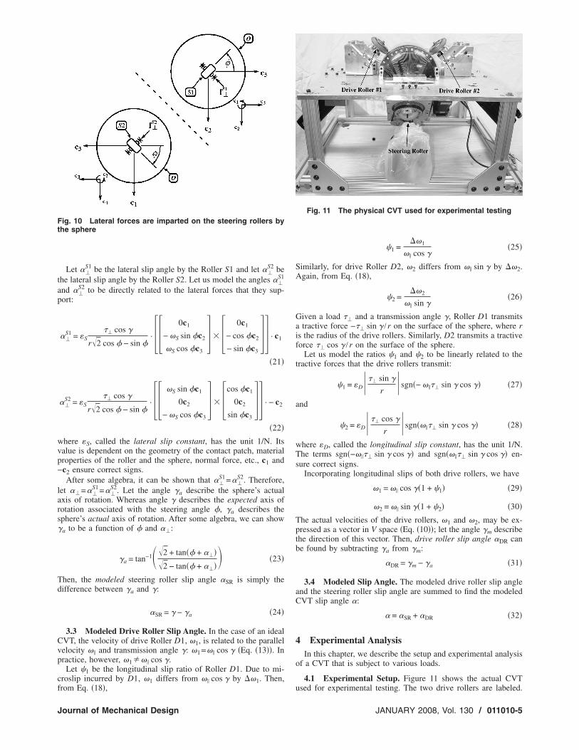
A load across the CVT ���� is supported internally within theCVT across four contacts between the sphere and the steering anddrive rollers. The two drive rollers support tractive forces in thedirection of rolling, and the two steering rollers support forceslateral to the direction of rolling �Fig. 10�.2
Let f�S1 be the lateral force imparted on the Roller S1 by the
sphere O. Then, from Ref. �7�, we know that f�S1 is a function of
�� and �:
f�S1 =
�� cos �
r�2 cos � − sin ��0c1 − cos �c2 − sin �c3�T �19�
where r is the radius of the steering rollers and � is the transmis-sion angle. To simplify the above algebraic expression, both � and� are used. Recall that � and � are related as described in Eq. �5�.
Let f�S2 be the lateral force imparted on the Roller S2 by the
sphere O. Then,
f�S2 =
�� cos �
r�2 cos � − sin ��cos �c10c2 sin �c3�T �20�
2
Fig. 9 Lateral slip angle ��
A summary of the internal forces within the CVT can be found in Ref. �7�.
Transactions of the ASME
tap
wvp−
lars�
Td
Cvp
cf
Ft
J
Let ��S1 be the lateral slip angle by the Roller S1 and let ��
S2 behe lateral slip angle by the Roller S2. Let us model the angles ��
S1
nd ��S2 to be directly related to the lateral forces that they sup-
ort:
��S1 = S
�� cos �
r�2 cos � − sin �· 0c1
− �S sin �c2
�S cos �c3 � 0c1
− cos �c2
− sin �c3 · c1
�21�
��S2 = S
�� cos �
r�2 cos � − sin �· �S sin �c1
0c2
− �S cos �c3 � cos �c1
0c2
sin �c3 · − c2
�22�here S, called the lateral slip constant, has the unit 1/N. Itsalue is dependent on the geometry of the contact patch, materialroperties of the roller and the sphere, normal force, etc., c1 andc2 ensure correct signs.After some algebra, it can be shown that ��
S1=��S2. Therefore,
et ��=��S1=��
S2. Let the angle �a describe the sphere’s actualxis of rotation. Whereas angle � describes the expected axis ofotation associated with the steering angle �, �a describes thephere’s actual axis of rotation. After some algebra, we can showa to be a function of � and ��:
�a = tan−1��2 + tan�� + ����2 − tan�� + ���
� �23�
hen, the modeled steering roller slip angle �SR is simply theifference between �a and �:
�SR = � − �a �24�
3.3 Modeled Drive Roller Slip Angle. In the case of an idealVT, the velocity of drive Roller D1, �1, is related to the parallelelocity �� and transmission angle �: �1=�� cos � �Eq. �13��. Inractice, however, �1��� cos �.
Let 1 be the longitudinal slip ratio of Roller D1. Due to mi-roslip incurred by D1, �1 differs from �� cos � by ��1. Then,
ig. 10 Lateral forces are imparted on the steering rollers byhe sphere
rom Eq. �18�,
ournal of Mechanical Design
1 =��1
�� cos ��25�
Similarly, for drive Roller D2, �2 differs from �� sin � by ��2.Again, from Eq. �18�,
2 =��2
�� sin ��26�
Given a load �� and a transmission angle �, Roller D1 transmitsa tractive force −�� sin � /r on the surface of the sphere, where ris the radius of the drive rollers. Similarly, D2 transmits a tractiveforce �� cos � /r on the surface of the sphere.
Let us model the ratios 1 and 2 to be linearly related to thetractive forces that the drive rollers transmit:
1 = D� �� sin �
r�sgn�− ���� sin � cos �� �27�
and
2 = D� �� cos �
r�sgn����� sin � cos �� �28�
where D, called the longitudinal slip constant, has the unit 1/N.The terms sgn�−���� sin � cos �� and sgn����� sin � cos �� en-sure correct signs.
Incorporating longitudinal slips of both drive rollers, we have
�1 = �� cos ��1 + 1� �29�
�2 = �� sin ��1 + 2� �30�The actual velocities of the drive rollers, �1 and �2, may be ex-pressed as a vector in V space �Eq. �10��; let the angle �m describethe direction of this vector. Then, drive roller slip angle �DR canbe found by subtracting �a from �m:
�DR = �m − �a �31�
3.4 Modeled Slip Angle. The modeled drive roller slip angleand the steering roller slip angle are summed to find the modeledCVT slip angle �:
� = �SR + �DR �32�
4 Experimental AnalysisIn this chapter, we describe the setup and experimental analysis
of a CVT that is subject to various loads.
4.1 Experimental Setup. Figure 11 shows the actual CVT
Fig. 11 The physical CVT used for experimental testing
used for experimental testing. The two drive rollers are labeled.
JANUARY 2008, Vol. 130 / 011010-5

Otrte
laaia
t
a
wC
vtrwio
d �a
b
Fv
0
nly one of the two steering rollers is visible. A servomotor, usedo generate CVT load, is directly coupled to each of the two driveollers. The drive rollers are 82a durometer in-line skating wheels;hey are 80 mm in diameter. The steering rollers are 84a durom-ter in-line skating wheels; they are 76 mm in diameter.
4.2 Testing Protocol. We are interested in finding the corre-ation between the CVT slip angle ���, velocity ���, transmissionngle ���, and load ����. In our experiments, the transmissionngles are set to values between −80 deg and +80 deg at 10 degncrements, and the CVT loads are set to values between −1.0 Nmnd 1.0 Nm at 0.1 Nm increments.
The CVT load is considered to be positive if the following isrue:
���1v1 + �2v2� � ��1v1 + �2v2�� � 0 �33�
nd negative if the following is true:
���1v1 + �2v2� � ��1v1 + �2v2�� � 0 �34�
4.3 Experimental Results. With the first set of experiments,e want to determine if there exists a correlation between theVT slip angle and the CVT velocity.In Fig. 12, we show the measured CVT slip angles �y axis�
ersus the CVT velocity �x axis� at various CVT loads with theransmission angle set to 45 deg. Figure 12 shows a lack of cor-elation between the CVT slip angle and CVT velocity3 and thuse may reasonably conclude that the measure of the slip angles is
ndependent of the CVT velocity �. We may, therefore, carry outur experimental analysis of the CVT at any CVT velocity.
4.3.1 Measured Slip Angle. The measured velocities of bothrive rollers may be expressed as vector � in the coordinate frame
�Fig. 7�. Let the angle �m describe the direction of this vectorFig. 7�. Then, the CVT slip angle � is the difference between thengle �m and the CVT angle �:
3Experimental results for other transmission angles also yield little correlation
ig. 12 CVT slip angle � versus CVT parallel velocity �¸ atarious CVT loads
etween � and CVT velocity.
11010-6 / Vol. 130, JANUARY 2008
� = �m − � �35�Figure 13 shows the measured CVT slip angle versus the CVTangle at CVT loads from −1 Nm to 1 Nm in 0.1 Nm increments.
4.3.2 Measured Steering Roller Slip Angle. The measuredsteering roller slip angle �SR can be found by measuring the dif-ference between the measured axis of rotation angle and the com-manded axis of rotation angle �also called the CVT angle� �Eq.�24��. We were able to determine the actual axis of rotationalangle visually, using a grid of closely spaced wires placed a fewmillimeters above the sphere. Figure 14 shows the measured steer-
Fig. 13 Measured �. CVT loads are between −1 Nm and 1 Nmin 0.1 Nm increments.
Fig. 14 Measured �SR
Transactions of the ASME
iv
st
atr
Noasrtcwmtcd
m1sa
5T
tab
il
Fa
J
ng roller slip angle �SR versus the commanded CVT angle � atarious CVT loads ��.
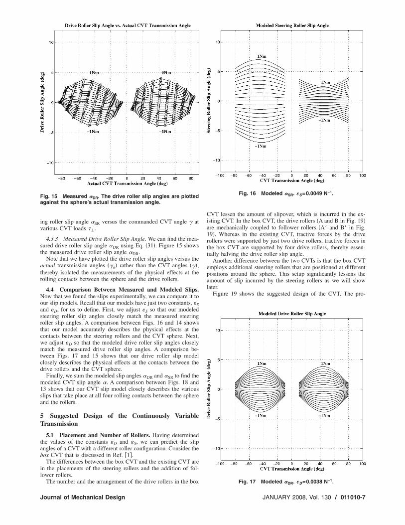
4.3.3 Measured Drive Roller Slip Angle. We can find the mea-ured drive roller slip angle �DR using Eq. �31�. Figure 15 showshe measured drive roller slip angle �DR.
Note that we have plotted the drive roller slip angles versus thectual transmission angles ��a� rather than the CVT angles ���,hereby isolated the measurements of the physical effects at theolling contacts between the sphere and the drive rollers.
4.4 Comparison Between Measured and Modeled Slips.ow that we found the slips experimentally, we can compare it tour slip models. Recall that our models have just two constants, Snd D, for us to define. First, we adjust S so that our modeledteering roller slip angles closely match the measured steeringoller slip angles. A comparison between Figs. 16 and 14 showshat our model accurately describes the physical effects at theontacts between the steering rollers and the CVT sphere. Next,e adjust D so that the modeled drive roller slip angles closelyatch the measured drive roller slip angles. A comparison be-
ween Figs. 17 and 15 shows that our drive roller slip modellosely describes the physical effects at the contacts between therive rollers and the CVT sphere.
Finally, we sum the modeled slip angles �DR and �SR to find theodeled CVT slip angle �. A comparison between Figs. 18 and
3 shows that our CVT slip model closely describes the variouslips that take place at all four rolling contacts between the spherend the rollers.
Suggested Design of the Continuously Variableransmission
5.1 Placement and Number of Rollers. Having determinedhe values of the constants D and S, we can predict the slipngles of a CVT with a different roller configuration. Consider theox CVT that is discussed in Ref. �1�.
The differences between the box CVT and the existing CVT aren the placements of the steering rollers and the addition of fol-ower rollers.
ig. 15 Measured �DR. The drive roller slip angles are plottedgainst the sphere’s actual transmission angle.
The number and the arrangement of the drive rollers in the box
ournal of Mechanical Design
CVT lessen the amount of slipover, which is incurred in the ex-isting CVT. In the box CVT, the drive rollers �A and B in Fig. 19�are mechanically coupled to follower rollers �A� and B� in Fig.19�. Whereas in the existing CVT, tractive forces by the driverollers were supported by just two drive rollers, tractive forces inthe box CVT are supported by four drive rollers, thereby essen-tially halving the drive roller slip angle.
Another difference between the two CVTs is that the box CVTemploys additional steering rollers that are positioned at differentpositions around the sphere. This setup significantly lessens theamount of slip incurred by the steering rollers as we will showlater.
Figure 19 shows the suggested design of the CVT. The pro-
Fig. 16 Modeled �SR. �S=0.0049 N−1.
−1
Fig. 17 Modeled �DR. �D=0.0038 N .JANUARY 2008, Vol. 130 / 011010-7

S D
Fig. 19 Suggested design of the box CVT
Fig. 20 Slip angles fo
011010-8 / Vol. 130, JANUARY 2008
posed CVT employs a pair of Rollers A and A� that are mechani-cally coupled. These two rollers transmit motions and torques to asingle rotational joint of a mechanical system, such as a robot.Rollers B and B� are also mechanically coupled; they both trans-mit motions and torques to a second rotational joint. Two sets of apair of steering rollers �each separated by a distance d� are locatedon opposite ends of the sphere.
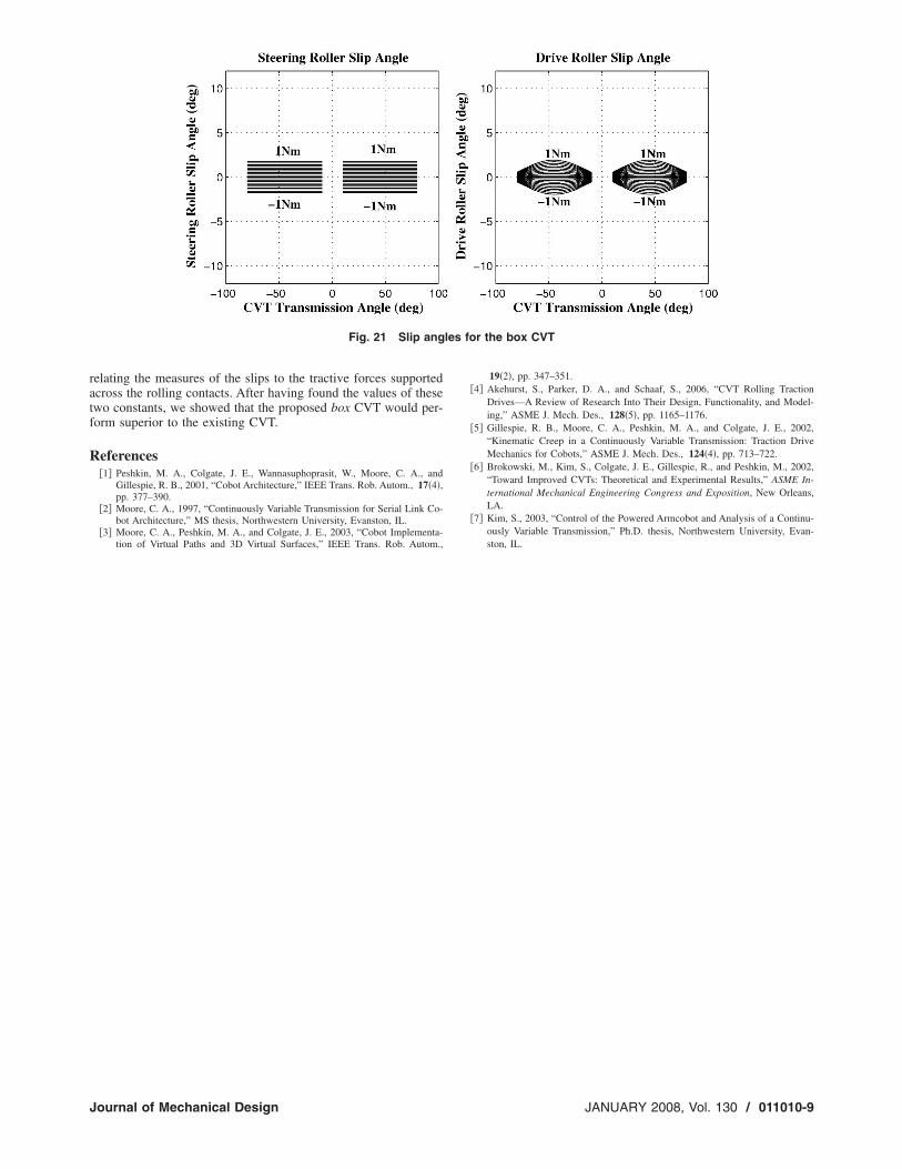
Let us assume that the box CVT employs the same types ofrollers and sphere as the existing CVT. Let us also assume that thepreload force is the same as it was for our experiment. We canthen predict the slip angles �, �SR, and �DR for the box CVT �withD=0.0038 N−1 and S=0.0049 N−1�.
Figure 20 shows the steering roller slip angles and the driveroller slip angles for the existing CVT �Fig. 2� and Fig. 21 showsthe slip angles for the box CVT. A comparison between Figs. 20and 21 shows that slip angles are smaller in the box CVT than inthe existing CVT.
The existing CVT employs two steering rollers to constrain thesphere to rotate about a particular axis of rotation, whereas thebox CVT employs four steering rollers to accomplish the sametask. A load across the CVT creates a moment about an axis thatmust be balanced by the tractive forces at the rolling contactsbetween the sphere and the steering rollers. Since the box CVTemploys more steering rollers than the existing CVT, they arerequired to support lesser tractive forces.
One other improvement over the existing CVT is the position ofthe steering rollers about the surface of the sphere. In the boxCVT, the steering rollers are positioned about the sphere such thattheir tractive forces produce the maximal moment about thesphere.
6 ConclusionIn this paper, we presented experimental results that showed
that loads across the CVT cause the velocities of the CVT joints todiffer from the intended velocities. Our experimental resultsshowed that for a particular transmission angle, the differencebetween the actual velocity ratio and the ideal velocity ratio islinearly related to the load applied across the CVT. We observedthat the cause of this difference is microslip at the rolling contactsbetween the sphere and the rollers. The CVT’s steering rollersincurred lateral slip, resulting in the sphere’s axis of rotation de-viating from the intended tilt angle. The CVT’s drive rollers in-curred longitudinal slip due to tractive forces that they had tosupport.
The lateral and longitudinal slips incurred by the steering anddrive rollers were characterized by two constants D and S, each
Fig. 18 Modeled �. � =0.0049 N−1, � =0.0038 N−1.
r the existing CVT
Transactions of the ASME
ratf
R
les
J
elating the measures of the slips to the tractive forces supportedcross the rolling contacts. After having found the values of thesewo constants, we showed that the proposed box CVT would per-orm superior to the existing CVT.
eferences�1� Peshkin, M. A., Colgate, J. E., Wannasuphoprasit, W., Moore, C. A., and
Gillespie, R. B., 2001, “Cobot Architecture,” IEEE Trans. Rob. Autom., 17�4�,pp. 377–390.
�2� Moore, C. A., 1997, “Continuously Variable Transmission for Serial Link Co-bot Architecture,” MS thesis, Northwestern University, Evanston, IL.
�3� Moore, C. A., Peshkin, M. A., and Colgate, J. E., 2003, “Cobot Implementa-tion of Virtual Paths and 3D Virtual Surfaces,” IEEE Trans. Rob. Autom.,
Fig. 21 Slip ang
ournal of Mechanical Design
19�2�, pp. 347–351.�4� Akehurst, S., Parker, D. A., and Schaaf, S., 2006, “CVT Rolling Traction
Drives—A Review of Research Into Their Design, Functionality, and Model-ing,” ASME J. Mech. Des., 128�5�, pp. 1165–1176.
�5� Gillespie, R. B., Moore, C. A., Peshkin, M. A., and Colgate, J. E., 2002,“Kinematic Creep in a Continuously Variable Transmission: Traction DriveMechanics for Cobots,” ASME J. Mech. Des., 124�4�, pp. 713–722.
�6� Brokowski, M., Kim, S., Colgate, J. E., Gillespie, R., and Peshkin, M., 2002,“Toward Improved CVTs: Theoretical and Experimental Results,” ASME In-ternational Mechanical Engineering Congress and Exposition, New Orleans,LA.
�7� Kim, S., 2003, “Control of the Powered Armcobot and Analysis of a Continu-ously Variable Transmission,” Ph.D. thesis, Northwestern University, Evan-ston, IL.
for the box CVT
JANUARY 2008, Vol. 130 / 011010-9