Graduate Theses and Dissertations Iowa State University Capstones, Theses and Dissertations

2020

Spreading information in social networks containing adversarial Spreading information in social networks containing adversarial

users users

Madhavan Rajagopal Padmanabhan Iowa State University

Follow this and additional works at: https://lib.dr.iastate.edu/etd

Recommended Citation Recommended Citation Rajagopal Padmanabhan, Madhavan, "Spreading information in social networks containing adversarial users" (2020). Graduate Theses and Dissertations. 18384. https://lib.dr.iastate.edu/etd/18384

This Dissertation is brought to you for free and open access by the Iowa State University Capstones, Theses and Dissertations at Iowa State University Digital Repository. It has been accepted for inclusion in Graduate Theses and Dissertations by an authorized administrator of Iowa State University Digital Repository. For more information, please contact digirep@iastate.edu.

Spreading information in social networks containing adversarial users

by

Madhavan Rajagopal Padmanabhan

A thesis submitted to the graduate faculty

in partial fulfillment of the requirements for the degree of

MASTER OF SCIENCE

Major: Computer Science

Program of Study Committee:Pavan Aduri, Co-major ProfessorSamik Basu, Co-major Professor

Jia(Kevin) Liu

The student author, whose presentation of the scholarship herein was approved by the program ofstudy committee, is solely responsible for the content of this dissertation/thesis. The GraduateCollege will ensure this dissertation/thesis is globally accessible and will not permit alterations

after a degree is conferred.

Iowa State University

Ames, Iowa

2020

Copyright c© Madhavan Rajagopal Padmanabhan, 2020. All rights reserved.

ii

TABLE OF CONTENTS

Page

LIST OF TABLES . . . . . . . . . . . . . . . . . . . . . . . . . . . . . . . . . . . . . . . . . . iv

LIST OF FIGURES . . . . . . . . . . . . . . . . . . . . . . . . . . . . . . . . . . . . . . . . . v

ACKNOWLEDGMENTS . . . . . . . . . . . . . . . . . . . . . . . . . . . . . . . . . . . . . . vi

ABSTRACT . . . . . . . . . . . . . . . . . . . . . . . . . . . . . . . . . . . . . . . . . . . . . vii

CHAPTER 1. OVERVIEW . . . . . . . . . . . . . . . . . . . . . . . . . . . . . . . . . . . . 11.1 Introduction . . . . . . . . . . . . . . . . . . . . . . . . . . . . . . . . . . . . . . . . . 11.2 Driving problem . . . . . . . . . . . . . . . . . . . . . . . . . . . . . . . . . . . . . . 21.3 Contributions . . . . . . . . . . . . . . . . . . . . . . . . . . . . . . . . . . . . . . . . 21.4 Organization . . . . . . . . . . . . . . . . . . . . . . . . . . . . . . . . . . . . . . . . 3

CHAPTER 2. REVIEW OF LITERATURE . . . . . . . . . . . . . . . . . . . . . . . . . . . 42.1 Diffusion Models . . . . . . . . . . . . . . . . . . . . . . . . . . . . . . . . . . . . . . 4

2.1.1 The Triggering Model . . . . . . . . . . . . . . . . . . . . . . . . . . . . . . . 42.1.2 Linear Threshold model . . . . . . . . . . . . . . . . . . . . . . . . . . . . . . 5

2.2 Influence Maximization (IM) Problem . . . . . . . . . . . . . . . . . . . . . . . . . . 72.3 Submodular functions . . . . . . . . . . . . . . . . . . . . . . . . . . . . . . . . . . . 72.4 Algorithms for estimating IM . . . . . . . . . . . . . . . . . . . . . . . . . . . . . . . 82.5 Estimating influence using Reverse Influence Sampling(RIS) . . . . . . . . . . . . . . 92.6 Variations of the IM problem and Related problems . . . . . . . . . . . . . . . . . . 10

CHAPTER 3. CONSTRAINED INFLUENCE MAXIMIZATION . . . . . . . . . . . . . . . 123.1 Theoretical analysis of CIM . . . . . . . . . . . . . . . . . . . . . . . . . . . . . . . 123.2 Algorithms for CIM . . . . . . . . . . . . . . . . . . . . . . . . . . . . . . . . . . . . 13

3.2.1 Natural Greedy Algorithm . . . . . . . . . . . . . . . . . . . . . . . . . . 143.2.2 Multi Greedy Algorithm . . . . . . . . . . . . . . . . . . . . . . . . . . . . . 163.2.3 An efficient Multi Greedy Heuristic . . . . . . . . . . . . . . . . . . . . . . 173.2.4 Efficient implementation with RIS . . . . . . . . . . . . . . . . . . . . . . . . 18

CHAPTER 4. EXPERIMENTS . . . . . . . . . . . . . . . . . . . . . . . . . . . . . . . . . . 204.1 Labelling Strategies . . . . . . . . . . . . . . . . . . . . . . . . . . . . . . . . . . . . 214.2 Experimental setup . . . . . . . . . . . . . . . . . . . . . . . . . . . . . . . . . . . . . 214.3 Experimental Observations . . . . . . . . . . . . . . . . . . . . . . . . . . . . . . . . 22

4.3.1 Comparison with Baseline Implementations. . . . . . . . . . . . . . . . . . . . 224.3.2 Budget vs. Influence. . . . . . . . . . . . . . . . . . . . . . . . . . . . . . . . 23

iii

4.3.3 Threshold vs. Influence. . . . . . . . . . . . . . . . . . . . . . . . . . . . . . 254.3.4 Target-Non-target Distribution vs. Influence. . . . . . . . . . . . . . . . . . . 264.3.5 Additive Loss. . . . . . . . . . . . . . . . . . . . . . . . . . . . . . . . . . . . 284.3.6 Runtime. . . . . . . . . . . . . . . . . . . . . . . . . . . . . . . . . . . . . . . 30

CHAPTER 5. SUMMARY AND FUTURE WORK . . . . . . . . . . . . . . . . . . . . . . . 315.1 Summary . . . . . . . . . . . . . . . . . . . . . . . . . . . . . . . . . . . . . . . . . . 315.2 Future Work . . . . . . . . . . . . . . . . . . . . . . . . . . . . . . . . . . . . . . . . 31

REFERENCES . . . . . . . . . . . . . . . . . . . . . . . . . . . . . . . . . . . . . . . . . . . . 32

iv

LIST OF TABLES

Page

Table 4.1 Datasets . . . . . . . . . . . . . . . . . . . . . . . . . . . . . . . . . . . . . . 20

Table 4.2 Target-Non-target Distribution vs. Influence for k = 20, θ = 10. Natural/Multi . . . . . . . . . . . . . . . . . . . . . . . . . . . . . . . . . . . . . . . 26

Table 4.3 Varying θ vs Additive Loss . . . . . . . . . . . . . . . . . . . . . . . . . . . . 28

Table 4.4 Additive Loss for varying budget . . . . . . . . . . . . . . . . . . . . . . . . 28

Table 4.5 Time taken(seconds) for Phase 1 . . . . . . . . . . . . . . . . . . . . . . . . 29

v

LIST OF FIGURES

Page

Figure 2.1 t = 0 . . . . . . . . . . . . . . . . . . . . . . . . . . . . . . . . . . . . . . . . 6

Figure 2.2 t = 1 . . . . . . . . . . . . . . . . . . . . . . . . . . . . . . . . . . . . . . . . 6

Figure 2.3 t = 2 . . . . . . . . . . . . . . . . . . . . . . . . . . . . . . . . . . . . . . . . 6

Figure 2.4 t = 3 . . . . . . . . . . . . . . . . . . . . . . . . . . . . . . . . . . . . . . . . 6

Figure 2.5 Illustration of diffusion in the IC model . . . . . . . . . . . . . . . . . . . . . 6

Figure 2.6 Submodularity under the IC model . . . . . . . . . . . . . . . . . . . . . . . 7

Figure 3.1 A sample graph for CIM problem . . . . . . . . . . . . . . . . . . . . . . . . 13

Figure 4.1 Budget vs. Influence for θ = 10. . . . . . . . . . . . . . . . . . . . . . . . . . 23

Figure 4.2 Budget vs Influence with θ = 10 on the LT Model . . . . . . . . . . . . . . . 24

Figure 4.3 Budget vs. Influence for θ = 10, clustered labeling. . . . . . . . . . . . . . . 25

Figure 4.4 Budget vs Influence with θ = 10 in the IC model with p = 0.1 . . . . . . . . 26

Figure 4.5 Threshold vs. Influence for Budget = 20. . . . . . . . . . . . . . . . . . . . . 27

Figure 4.6 Overall Time Taken 80% Targets, θ = 10 under the IC Model with p =1/inDeg . . . . . . . . . . . . . . . . . . . . . . . . . . . . . . . . . . . . . . 30

vi

ACKNOWLEDGMENTS

I am deeply indebted to my advisors Dr. Pavan Aduri and Dr. Samik Basu for their constant

guidance, support, and encouragement that made this work possible. I also wish to thank Dr. Jia

(Kevin) Liu for his supervision and insightful discussions.

I would like to recognize the support provided by the Department of Computer Science at

Iowa State University. My graduate study and research was funded in part through Teaching

Assistantships.

I am grateful to the National Science Foundation (NSF) for supporting this work in part through

grants CCF 1421163 and CCF 1555780.

vii

ABSTRACT

In the modern day, social networks have become an integral part of how people communicate

information and ideas. Consequently, leveraging the network to maximize information spread

is a science that is applied in viral marketing, political propaganda. In social networks, an

idea/information starts from a small group of users (known as seed users) and is propagated

through the network via connections of the seed users. There are limitations on the number of

seed users that can be convinced to adopt a certain idea. Therefore, the problem exists in finding

a small set of users who can maximally spread an idea/information. This is known as the influence

maximization problem. While this problem has been studied extensively, the presence of potential

adversarial users and their impact on the information spread has not been considered in existing

solutions.

In this thesis, we study the problem of spreading information to Target users while limiting the

spread from reaching adversarial(Non Target) users. To this end, we consider a hard constraint -

the objective is to maximize the information spread among the Target users while the number of

Non-Target users to whom the information reaches is limited by a hard constraint. We design two

algorithms - Natural Greedy and Multi Greedy with efficient RIS based implementations.

We run our solutions on real-world social networks to study the information spread. Finally, we

evaluate the quality of our solutions on different models of diffusion and network settings.

1

CHAPTER 1. OVERVIEW

Social networks have developed into an essential mode of communication in modern day to day

life. By providing a platform, whose use can range from sharing funny memes to coordinating

relief efforts in times of crisis, social networks have demonstrated to be a highly effective tool for

communicating information. Naturally, it would be beneficial to leverage the network to control

and spread information of our choice. Diffusion is the process via which information spreads across

users in the network. Each user is capable of ”influencing” others connected to him/her. If a user

is successful in influencing his/her immediate connections, then each of the newly influenced users

can pass along the information to their connections. Given the scale of these networks and the

seemingly uncertain way in which information spreads, controlling the spread of information poses

interesting challenges. The presence of users who are adversarial to the information that is being

spread adds further challenges to the problem.

1.1 Introduction

In trying to spread information, a natural problem arises: How to find an initial set of users

(seed) of a specific number (determined by budget k) that can maximally spread the information in

the network. This is called the Influence Maximization (IM) problem. Kempe et al. [14] posed this

as a discrete optimization problem under the Independent Cascade and Linear Threshold models of

diffusion. Under these models, they proved that the IM problem is NP-hard and designed a greedy

algorithm that provided a 1−1/e-approximation guarantee on the quality of the solution. For a set

of users S, σ(S) is the expected number of users influenced in the network. The greedy algorithm

builds a solution that iteratively adds a user that can maximally increase the influence function

σ(S). However, given a user (or a set of users), computation of that user’s expected influence is

a #P-hard problem. Therefore, the greedy algorithm is practically infeasible. This has led to the

2

development of various heuristics and probabilistic algorithms that scale to real world networks

[24, 5, 30, 29].

Li et al. [19] consider a variant of the IM problem where the goal is to maximize the information

spread to a subset of targeted users in the network. In our work, in addition to Target users, we

consider the presence of Non-Target users and place a hard constraint on the number of Non-Target

users that can be influenced.

1.2 Driving problem

In social networks, in addition to users that we would like to influence, there are users present

that would negatively impact our objective. We observe that this problem appears in several

scenarios in marketing, political propaganda, etc. During political campaigns, we would like to

run ads that maximally reach users sympathetic to our cause. If the ads were to reach users with

opposing viewpoints, it may inadvertently mobilize those users causing a negative reaction to our

campaign. In another scenario, consider an online marketing campaign that advertises an alcoholic

beverage. Not only would it be unethical to have the advertisement reach under-age users, but it

may be a potential violation of terms of service and/or the law.

Considering these scenarios, we study the problem of Influence Maximization in the presence of

adversarial users. Consider a social network modeled as G = (V,E). Suppose we classify the users

into two categories - Targets and Non-Targets. Given a threshold θ, the objective is to find a seed

set S of size k such that the influence among the Target users is maximized, while at the same time

the number of Non-Target users influenced is kept below θ. We call this the Constrained Influence

Maximization Problem.

1.3 Contributions

We study the Constrained Influence Maximization problem [27, 25]. We review the Natural

Greedy and Multi Greedy algorithms for CIM problem. We apply RIS based sketching to

the Natural Greedy and Multi Greedy Algorithms. We evaluate the algorithms on real-

3

world social networks with various Target, Non Target labelling strategies. We present extensive

experiments of RIS based sketching under the Linear Threshold, Independent Cascade models of

diffusion. Finally, we experimentally evaluate the Additive Loss - the additive approximation error

of the Natural Greedy algorithm.

1.4 Organization

The rest of this thesis is organized as follows. Chapter 2 provides a review of current work in

Influence Maximization and terminology. Chapter 3 describes the CIM problem and the Natural

Greedy , Multi Greedy algorithms. Chapter 4 presents the experimental design and results.

Finally, Chapter 5 presents our conclusion and future extensions.

4

CHAPTER 2. REVIEW OF LITERATURE

The Influence Maximization problem seeks to find a set of highly influential users in a social

network. The idea is to use these highly influential users as a seed to propagate information that

reaches the maximum possible users in the network. The immediate question that arises is - How

can this spread of information be characterized? On the outset, this appears to be a probabilistic

process. Given a user(s), how can we determine who this user(s) will probably influence? This

question is addressed by various Diffusion models.

2.1 Diffusion Models

Suppose a set of users(seed) have initially adopted some information. The information is adopted

by users that are influenced by the seed users, and propagates through the network. This eventually

reaches its completion, resulting in a final set of active/influenced users. This process is termed as

diffusion. Diffusion models attempt to characterize the mechanism via which information spreads

from one node to the neighbors. Each diffusion model comprises of the following: 1) A seed set of

users who have initially adopted the information, 2) A well-defined criterion under which each user

can influence another, and 3) The diffusion terminates after a finite number of steps resulting in a

final set of influenced users.

2.1.1 The Triggering Model

First proposed by Kempe et al. [14], the Triggering Model defines the notion of Triggering

sets of a user v. The idea is that each user has a subset of neighbors, who can trigger the user

into adopting an idea. For a diffusion process, each user v randomly selects a subset Tv from its

neighbors (based on some distribution). The diffusion starts with seed users S who are initially

5

activated. At time step t, v is activated if Tv is active at time step t− 1. This goes on until there

can be no more newly activated users.

There are two instances of the Triggering Model that are widely used - the Independent Cas-

cade(IC) and Linear Threshold(LT) model.

2.1.1.1 Independent cascade model

Let’s consider the social network as a graph G = (V,E). V represents the set of users and a

directed edge is placed between two users if one user can influence the other. In the Independent

Cascade model, each edge is assigned a propagation probability - p(u, v). This value represents

the probability with which node u can influence v. At time step 0, S ⊆ V is the seed set that is

activated. At the next time step, each newly activated node u can activate its immediate inactive

neighbors with probability p(u, v). If u fails to activate v, then v can no longer be activated by

edge (u, v). Every newly activated node tries to activate its inactive neighbors in the next time

step. This process continues until there are no longer any nodes that can be activated.

Figure 2.5 illustrates this process. The graph consists of 7 nodes, numbered 1 to 7. At time

step 0, the diffusion starts with the seed set {1}. 1 succeeds in activating 3 as the propagation

probability is 1.0. Suppose 1 fails to activate 2 as p(1, 2) = 0.01. Then, at time step 1, the active

nodes are {1, 3}. This continues until time step 3, resulting in the active node set {1, 3, 4, 5, 6, 7}.

Propagation probability In the IC model, for an incoming edge to v, a common choice

for the propagation probability is 1/inDeg(v) where inDeg(v) is the number of nodes that have a

directed edge to v. The resulting model is termed as Weighted Cascade model [14]. Other choices

for p include constant values(p = 0.01 or p = 0.1) [5, 9]. Another variation is the Trivalency model

in which each edge is assigned a probability randomly from {0.1, 0.01, 0.001} [4].

2.1.2 Linear Threshold model

Let N in(v) be the set of vertices such that u ∈ N in(v) iff there exists an edge (u, v) ∈ E.

Let N inact(v) be the set of vertices such that u ∈ N in

act(v) iff there exists an edge (u, v) ∈ E and

6

1

2

3

4 5

6

7

0.01

1.0

0.4

0.9 0.9

0.01

1.0

0.7

1.0

Figure 2.1: t = 0

1

2

3

4 5

6

7

0.01

1.0

0.4

0.9 0.9

0.01

1.0

0.7

1.0

Figure 2.2: t = 1

1

2

3

4 5

6

7

0.01

1.0

0.4

0.9 0.9

0.01

1.0

0.7

1.0

Figure 2.3: t = 2

1

2

3

4 5

6

7

0.01

1.0

0.4

0.9 0.9

0.01

1.0

0.7

1.0

Figure 2.4: t = 3

Figure 2.5: Illustration of diffusion in the IC model

u is activated. In the linear threshold model, every edge is assigned a weight w(u, v) such that

∀v,∑

u∈N in(v)w(u, v) ≤ 1. Each node v randomly selects a threshold θv in the interval [0, 1]. Like

the IC model, this model operates in discrete time steps with the seed set S initially activated at

time step 0. At each time step t, a node v is activated if∑

u∈N inact(v)

w(u, v) ≥ θv. The process

completes in a finite number of time steps.

Choice of w(u, v) : A popular choice for assigning the weights for incoming edges to v is to

randomly select a value ∈ [0, 1] and normalize it so that∑

u∈N in(v)w(u, v) = 1 [6, 30]. Another

choice for w(u, v) is 1/inDeg(v).

7

2.2 Influence Maximization (IM) Problem

The Influence Maximization problem is a discrete optimization problem first proposed by Kempe

et al. [14]. Let the social network be represented as a graph G = (V,E). LetM represent a diffusion

model. For any S ⊆ V , let σ(S) be the expected number of nodes influenced by S under M. The

Influence maximization problem is defined as follows:

Problem 1. Given a network G = (V,E), k and a diffusion model M, compute S ⊆ V where

|S| ≤ k such that σ(S) is maximized.

Kempe et al. [14] proved that Problem 1 is a monotone non-decreasing submodular function

under the Triggering model and by extension, the IC and LT models. Below, we present a review

of these concepts.

2.3 Submodular functions

A function f : 2V → R is called submodular if and only if ∀A,B ⊆ V , f(A) + f(B) ≥

f(A ∪B) + f(A ∩B) [22]. Equivalently, a function is submodular if and only if ∀A ⊆ B ⊆ V and

e /∈ B, f(A∪ {e})− f(A) ≥ f(B ∪ {e})− f(B). The second definition provides an intuition on the

diminishing returns property of submodular functions. The element {e} provides a higher gain on

the smaller set A than on the bigger set B. We refer to the value f(A∪{e})−f(A) as the marginal

gain denoted by f(e|A).

Monotone non-decreasing submodular functions A submodular function f : 2V → R is

monotone non-decreasing if ∀A ⊆ V , f(A) ≤ f(A ∪ {e}).

3

1 2

1.0 1.0

Figure 2.6: Submodularity under the IC model

8

Let’s interpret this in the context of the IM problem using figure 2.6. In this graph, there are

three nodes and the diffusion occurs as per the IC model. σ({1}) = 2 as the activated set will be

{1, 3}. Similarly, σ({2}) = 2 as the activated set will be {2, 3}. Observe that σ({2}|{1}) = 1 ≤

σ({2}|φ). In this case, {2} can influence only one additional node(itself) since 1 will have already

influenced {1, 3}.

2.4 Algorithms for estimating IM

The primary challenge in solving the IM problem lies in the computation of the influence

function σ(S). The exact computation of σ(S) is known to be a #P-hard problem. Therefore, we

resort to estimations of σ(S). Kempe et al. [14] used a simulations based approach to estimate

σ(S). In each iteration of the Greedy Algorithm, a large number of simulations (typically ∼ 10000)

is performed to find the node that maximally increases σ. More precisely, if Si is the seed set built

at the ith iteration, ∀v ∈ V \S, σ(S∪{v}) is estimated by performing simulations. Naturally, this is

computationally expensive even in small graphs. Leskovec et al. [18] developed the Cost Effective

Lazy Forwarding(CELF) algorithm that exploited the submodularity of the objective function to

significantly reduce the number of candidate nodes considered in each iteration. The underlying

idea of CELF is that for two nodes u,v: if σ(u|Si) ≥ σ(v|Si) and σ(u|Si+1) ≥ σ(v|Si), then there

is no need for computing σ(v|Si+1). Based on this observation, they construct a Max Heap that

has the node with the maximum marginal gain at the top. If this node’s gain is outdated w.r.t. the

current seed, an update is made and the heap is reconstructed. In practice, this greatly reduces

the number of vertices that are considered in the Greedy algorithm.

Ohsaka et al. [24] introduced a Pruned Monte Carlo Simulations-based algorithm under the IC

model that further scales the Greedy algorithm without compromising the quality of the solution.

Their algorithm works by constructing a large number of live edge graphs( 10000) by retaining each

edge with probability p(e). For each of these graphs, their algorithm constructs Directed Acyclic

Graph(DAG). Each node in the DAG is a strongly connected component in the live edge graph

and the node with the maximum degree is used as a hub. They track descendants and ancestors of

9

the hub in each of the DAGs. The algorithm performs a pruned BFS to calculate the influence of

an ancestor node of the hub by not visiting the descendants of the hub. This technique significantly

speeds up the simulation.

Several heuristic algorithms have also been developed that are designed for practical efficiency

but lack theoretical guarantees. Chen et al. [5] designed the DegreeDiscountIC algorithm for

the IC model with small propagation probability. DegreeDiscountIC initially adds the vertex

that has the highest outdegree seed. The degrees of its immediate neighbors are discounted based

on p, following which the next best vertex is selected. Jung et al. [13] developed the Influence

Ranking Influence Estimation (IRIE) algorithm. They develop a system of linear equations, whose

solution is used as an estimation of the influence of each vertex. At each iteration of the algorithm,

they modify the linear equations and get an update the estimates based on the seed set.

Borgs et al. [2] developed the idea of Reverse Influence Sampling(RIS), which is to generate

random reverse reachable(RR) sets. Using these sets to estimate the influence, they develop a

(1 − 1e − ε)- approximate algorithm. Tang et al. [30, 29] extended this idea and developed TIM,

TIM+, and IMM algorithms. Their algorithms reduce the runtime by attempting to generate a

minimal number of RR Sets without losing the approximation guarantee. Nguyen et al. [23]

developed SSA, D-SSA algorithms that attempt to further improve on IMM by further reducing

the number of RR sets. However, Huang et al. have pointed out that D-SSA may not retain the

theoretical approximation guarantee. An extensive study of these algorithms can be found in Li et

al.’s [31] survey paper.

2.5 Estimating influence using Reverse Influence Sampling(RIS)

In recent years, there have been several proposed methods to estimate σ(S) [9, 24, 5]. In

this thesis, we use the Reverse Influence Sampling(RIS) method that generates random reverse

reachable sets, first introduced by Borgs et al. [2]. To generate a random reverse reachable set

under the IC model, first randomly select a vertex v. Then retain each edge in the graph according

to its propagation probability p(e). The random RR set is the set of vertices that are reachable on

10

this graph by doing a reverse BFS starting at v. Let R be a random RR set and n be the number

of vertices in the graph. For any S ⊆ V , Borgs et al. proved that σ(S) = n × Pr[S ∩ R]. Tang

et al. [30] extended the notion of random RR sets to the LT model. In our experiments, we have

used Tang et al.’s [30] method to generate RR sets in the IC and LT model.

2.6 Variations of the IM problem and Related problems

Since its introduction, significant work has been done on the Influence Maximization problem

while also considering additional contexts. The works of [1, 3] address topic-aware influence max-

imization. In this variation, a user’s probability of influencing a connected user is also dependent

on the topic that is being propagated. The problem is then to find k influential users that can

convince the maximum number of people to adopt a certain topic. Another related approach to

this problem is to model the likelihood with which a user will adopt a certain topic irrespective of

from whom it comes from [20]. Fu et al. [7, 8] study how strongly (or weakly) a user is influenced,

and term it as Attitude of the user. They study the Attitude Maximization Problem, where the

objective is to maximize the overall attitude of the network.

A variant that has been well studied is that of targeted influence maximization [19, 17]. Here

a subset of nodes of the network are labeled as target nodes. The goal is to find a seed set of size

k that influences the maximum number of target nodes. Li et al. [20] similarly have considered

targeted influence maximization, where the targets are identified using keywords. On the other

hand, Song et al. [28] considered targeted influence maximization within specific time steps. When

the target set is a singleton, it is referred to as personalized influence maximization [10]. None

of these works consider non-target nodes and the constraint that the number of non-target nodes

that are influenced is below a pre-determined threshold. In these works, any node that is not

a target does not negatively impact the influence maximization question–rather non-target nodes

may be used to propagate the influence to more target nodes. In contrast, we introduce the concept

of non-targets that must not be influenced—more specifically, the expected number of non-targets

influenced must remain within a threshold. Intuitively, this brings in the new challenge of balancing

11

diffusion between non-targets and targets to maximize the targeted influence while satisfying the

hard constraint of keeping the non-target influence below the threshold. The theoretical implication

of such a challenge is that the diffusion function no longer remains submodular and monotonic,

thus making the standard approximation guarantee of the greedy algorithm invalid. This is in

contrast with the targeted influence maximization where the objective function is submodular and

monotone.

Parallel to maximizing the spread of information, significant advances have been made in dis-

rupting information spread in social networks [15, 16]. In these problems, nodes or edges are

deleted in social networks in order to limit the spread of information. In the Constrained Influence

Maximization problem, we limit the spread of information to adversarial users rather than disrupt

information cascades originating from such users.

Iyer and Bilmes [12] introduced the Submodular Cost Submodular Knapsack(SCSK) problem.

Given monotone, non-decreasing submodular functions f ,g and a budget b - the objective is to find

a set X that maximizes f(X) such that g(X) ≤ b. They leverage surrogate functions for f ,g and

develop iterative algorithms with approximation guarantees for SCSK. Although SCSK is similar

to our Constrained Influence Maximization problem, SCSK differs by not imposing a size constraint

on X.

12

CHAPTER 3. CONSTRAINED INFLUENCE MAXIMIZATION

We study the problem of Influence Maximization in the presence of adversarial users. Consider

a social network modelled as G = (V,E). Let each user be labelled Target or Non Target leading

to subsets T ⊆ V and N = V \ T . Let σT (S) and σN (S) be the expected number of Target and

Non Target users influenced by S. Let σθT (S) = σT (S) if σN (S) ≤ θ. If σN (S) > θ, σθT (S) = 0. The

Constrained Influence Maximization (CIM) problem, first formalized in [27], is defined as follows:

Problem 2. Given a network G = (V,E, T,N) and k, θ, compute S ⊆ V where |S| ≤ k such that

σθT (S) is maximized.

Figure 3.1 provides an illustration of this problem. v1 to v8 are labelled either T or N . For

k = 2, θ = 2, the optimal solution S∗ = {v3, v5} leading to σθT (S∗) = 7. If we label all the nodes as

Targets, the problem becomes an instance of the standard Influence Maximization problem. Due to

this reduction, we conclude that CIM is NP-Hard. We can also generalize the problem formulation

to include Neutral nodes i.e. nodes that are either Target or Non Target. It is immediate that these

Neutral nodes neither contribute to σT (S) nor σN (S). Thus, these Neutral nodes do not affect our

objective function σθT (S).

3.1 Theoretical analysis of CIM

The greedy algorithm for the standard Influence Maximization problem provides a (1 − 1/e)-

approximate solution. However, this approximation guarantee relies on the fact that the objective

function σ(S) is non-negative, monotone non-decreasing, and submodular [14, 22]. We find that

our objective function is neither monotone nor submodular.

Lemma 3.1.1. The objective function of CIM , σθT (S), is non-monotone and non-submodular.

Proof. Suppose we have G = (V,E) and S ⊆ V such that σT (S) = a > 0 and σN (S) ≤ θ. Thus

σθT (S) = a. If there exists a node u such that σN (S ∪ {u}) > θ, then σθT (S ∪ {u}) = 0. Therefore,

13

T

v1

N

v2

T v3

T

v4

T

v5

N

v6

T

v7

N

v81.0

1.0

1.0

0.01

1.0

1.01.0

1.0

1.0

Figure 3.1: A sample graph for CIM problem

σθT (S) is non-monotone. In the same example, we observe that σθT ({u}|S) = −a. Let there be

another node v such that σN (S ∪ {v}) > θ leading to σθT (S ∪ {v}) = 0. Now, σθT ({u}|S ∪ {v}) = 0.

This violates submodularity as the marginal gain of u on the smaller set S is less than the marginal

gain on the bigger set S ∪ {v}.

We showed that CIM problem is NP-hard. In fact, obtaining a constant-factor approximation

algorithm for CIM is quasi NP-hard.

Theorem 3.1.2. [25] For every 0 ≤ c ≤ 1, if there is a polynomial-time, c-approximation algorithm

for the CIM problem in the IC model, then every problem in NP can be solved in O(nlogk n) time

for some k ≥ 1.

The proof of Theorem 3.1.2 can be found in [25].

3.2 Algorithms for CIM

Despite the above property of the objective function, we find that the greedy algorithm still

provides an additive approximation guarantee within a multiplicative factor of (1 − 1/e) and an

additive error. We present the following three algorithms [27, 25]:

1. Natural Greedy Algorithm

14

2. Multi Greedy Algorithm

3. An efficient Multi Greedy Heuristic algorithm

3.2.1 Natural Greedy Algorithm

Algorithm 1 Natural Greedy Algorithm [27, 25]

1: procedure Natural Greedy (G = (V,E,L), k, θ)

2: S = φ

3: while |S| ≤ k do

4: S = S ∪ {arg maxv σθT (S ∪ {v})}

5: end while

6: return S

7: end procedure

The Natural Greedy algorithm iteratively builds a seed set S by adding a vertex v that

maximally increases σT while ensuring that by adding v σN does not exceed θ. We establish

two approximation guarantees provided by the Natural Greedy algorithm. To characterize the

guarantees, we establish the following notations:

• OPTk,θ - Optimal solution to CIM for budget k, threshold θ.

• BestGainθ = max{σ2θT (v) | v ∈ V }

• Given S,R ⊆ V , gainS(R, θ) = σθT (S∪R)−σθT (S) if σN (S∪R) ≤ θ. Otherwise, gainS(R, θ) =

0.

• LeastGainθ - the minimum value of gainS({v}, θ) over all S of size at most k and v.

• Diffθ = BestGainθ − LeastGainθ

Diffθ captures the difference between the maximum increase in targets influenced that is caused

by a single node v and the minimum increase in targets influenced that is caused by a single node.

Based on Diffθ, we claim the first approximation guarantee.

Theorem 3.2.1. [25]

σT (Sk) ≥ (1− 1/e)[OPTk,θ]− k ×Diffθ.

15

The proof of Theorem 3.2.1 can be found in [25].

Our second approximation guarantee refines the additive approximation factor −k × Diffθ.

Consider the set Si−1 that is built after i−1 iterations. Let u′ = argmaxu∈V \Si−1{σ2θT (Si−1∪{u})}.

u′ is the best node that can be added to Si−1 which would influence at most 2θ non targets. Let

S′i = Si−1 ∪ u′. Note that Natural Greedy builds Si by adding the best node to Si−1 such that

Si influences at most θ non targets. In contrast, S′i influences at most 2θ non targets. We refer to

the following lemma from Equation 2 in [25].

Lemma 3.2.2. [25]

OPTk,θ − σ2θT (S′i+1) ≤k − 1

k(OPTk,θ − σθT (Si)) (3.1)

Proceeding further, for any S such that σN (S) ≤ θ and η ≥ θ, define:

BestG(S, η) = max{σηT (S ∪ {u})− σθT (S)|u ∈ V }

BestG(S, η) represents the best possible increase to the number of targets influenced by adding

a single node u subject to the constraint that the number of non targets influenced is at most η.

Let OPTk,θ be the optimal solution to CIM for budget k, threshold θ. The Natural Greedy

algorithm provides a solution that has an additive error in relation to BestG(S, η).

Theorem 3.2.3. [25]

σθT (Sk) ≥ (1− 1/e)[OPTk,θ]− (k−1∑i=0

BestG(Si, 2θ)− σθT (Sk))

Proof. Note that, from the definition of S′i+1 (best possible extension to Si with the threshold 2θ),

we have

σ2θT (S′i+1) = σθT (Si) +BestG(Si, 2θ) (3.2)

Since Si+1 is obtained from Si in greedy manner,

σθT (Si+1) = σθT (Si) +BestG(Si, θ) (3.3)

From above two equalities, we obtain

σ2θT (S′i+1)− σθT (Si+1) = BestG(Si, 2θ)−BestG(Si, θ) (3.4)

16

Combining this with Lemma 3.2.2, we obtain:

OPTk,θ − σθT (Si+1) ≤ (1− 1/k)[OPTk,θ − σθT (Si)]

+ BestG(Si, 2θ)−BestG(Si, θ)

Solving the above recurrence yields our theorem.

Henceforth, we will refer to∑k−1

i=0 BestG(Si, 2θ) − σθT (Sk) as the Additive Loss. Consider the

following: if at each iteration in the Natural Greedy algorithm, we are allowed to add a node that

can influence at most 2θ non targets, the total gain that we can obtain with these nodes compared

to the nodes that we actually select is the Additive Loss. The Natural Greedy algorithm can

be implemented in O(k × |V | × Inf), where Inf indicates the runtime complexity of influence

computation.

3.2.2 Multi Greedy Algorithm

Algorithm 2 Multi Greedy Algorithm [27, 25]

1: procedure Multi Greedy (G = (V,E, L), k, θ)

2: MG0 = {φ}, i=0

3: while i < k do

4: for all S ∈MGi do

5: NT = σN (S)

6: for j = NT to θ do

7: umax = arg maxu σjT (S ∪ {v})

8: S′ = S ∪ umax9: Add S′ to MGi+1

10: end for

11: end for

12: i = i+ 1

13: end while

14: return arg maxS∈MGkσθT (S)

15: end procedure

The Multi Greedy algorithm tracks multiple seed sets at each iteration. Let r be the number

of sets tracked at the ith iteration: S1i , S

2i ..S

ri . For l = 1 to r, let σN (Sli) = NTl. For each of these

sets, extend the set by at most θ many ways: For each j = NTl to θ, find a vertex umax such that

17

σT (Sli ∪ {u}) is maximized while σN (Sli ∪ {u}) = j. At the (i+ 1)th iteration, these newly formed

sets are extended the same way until we reach sets of size k. Finally, the algorithm returns the set

that hits the maximum number of targets as the solution.

Observe that the Multi Greedy algorithm will track the seed set built by the Natural

Greedy algorithm. Therefore, σθT (MG) ≥ σθT (NG). In general, we cannot show that Multi

Greedy outperforms Natural Greedy in all instances. Consider the following example: Suppose

for a graph G = (V,E) and θ, there does not exist any vertex u whose σN (u) < θ. In this case, the

output of Multi Greedy will be the same as the output of Natural Greedy .

We run into a practical hurdle with Multi Greedy . The algorithm keeps track of O(θk) seed

sets. Therefore, this is computationally infeasible.

3.2.3 An efficient Multi Greedy Heuristic

Due to the impractical nature of Multi Greedy Algorithm, we design a heuristic that will

reduce the number of seed sets tracked from O(θk) to O(θ). The Multi Greedy heuristic [27, 25]

works in two phases:

3.2.3.1 Phase 1

For every vertex v ∈ V , compute σN (v) and store it in a set Ai if σN (v) = i. This results in

the construction of (θ + 1) sets: Ai, for i = 0 to θ.

3.2.3.2 Phase 2

In this phase, we construct a tree that we shall refer to as IMTree. At the root of the tree, we

have a dummy node r and σT (r) = σN (r) = 0. For a node n in the tree, we will use IMSeed(n)

to refer to the set composed of the vertices in a path from n to the root r (not including r). Let

modN (S) =∑

u∈S σN (u). Starting from the root, perform the following operation:

18

1. For every leaf node u in the IMTree: For each i from modN (IMSeed(u)) to θ, find v that

maximally increases σT (IMSeed(u)∪ {v})such that modN (IMSeed(u)∪ {v}) = i and add v

as a child node to u.

2. Let Mj denote a set of newly added nodes such that ∀vnew ∈Mj ,modN (IMSeed(vnew)) = j.

For each i from 0 to θ perform the following operation: Retain arg maxm∈MiσT (IMSeed(m))

and prune every other node in Mi from the IMTree. This leaves at most (θ+ 1) new nodes

added to the IMTree. If no new nodes are added, terminate.

3. If the height of the IMTree is k, terminate. Otherwise, go to Step 1.

For all nodes at level k, find the node nmax that maximizes the expected targets influenced i.e.

nmax = arg maxσT (IMSeed(n)). Output IMSeed(nmax) as the solution. Observe that we use

modN (S) =∑

u∈S σN (u) as an approximation of σN (S). If modN (S) ≤ θ then σN (S) ≤ θ due to

σN being a submodular function. Additionally, we use the values calculated in phase 1 to compute

modN . Henceforth, Multi Greedy will refer to the Multi Greedy heuristic algorithm.

3.2.4 Efficient implementation with RIS

Borgs et al. [2] introduced Reverse Influence Sampling (RIS), an efficient way to estimate σ(S)

and solve the Influence Maximization problem under the IC model. RIS defines the notion of

reverse reachable(RR) sets, using which σ(S) can be estimated. Tang et al. [30] extended the

notion of RR sets to the LT model. The following lemma is first proved by Borgs et al. [2].

Lemma 3.2.4. ( [2], Observation 3.2) Let n be the number of nodes in Graph G = (V,E). Let

g ∼ G be a random graph that is drawn by keeping each edge with probability pe. Let u ∼ V be a

random vertex chosen from V . Let RgT (u) represent the set of nodes that can be reached by u in gT .

We term RgT (u) as a Reverse Reachable set. For any S ⊆ V , σ(S) = nPu∼V,g∼G[RgT (u)∩S 6= φ].

19

Note that pe varies based on the influence model. For our problem, we need to estimate

σT (S), σN (S). Let’s modify the proof of Lemma 3.2.4 slightly to allow us to estimate σT (S) (or

σN (S)). Let T ⊆ V be the targets.

σT (S) =∑u∈T

Pg∼G[∃v s.t v ∈ S and v ∈ RgT (u)]

= |T | ×∑u∈T

1

|T |· Pg∼G[∃v s.t v ∈ S and v ∈ RgT (u)]

= |T | × Pu∼T,g∼G[∃v s.t v ∈ S and v ∈ RgT (u)]

(3.5)

A similar observation can be made for σN (S). Using Chernoff Bounds [2], for any v, with

high probability, we can estimate σT (v) (or σN (v)) within an error ε, by generating O(n log n/ε2)

number of RR sets .

3.2.4.1 Natural Greedy and Multi Greedy using random RR sets

Natural Greedy : For the greedy implementation, we generate O(kn log n/ε2) number of

RR sets for Targets and Non Targets respectively. To find the best seed set, find S that covers the

maximum number of RR sets .

Multi Greedy : For Phase 1, generate O(n log n/ε2) number of RR sets for Non Targets. In

Phase 2, we keep track of (θ+ 1) seed sets. A naive implementation of Multi Greedy would keep

track of O(θknlogn/ε2) RR sets for Targets, each of which corresponds to a branch in the IMTree.

We resolve this by doing the following: Generate O(kn log n/ε2) Target RR sets . For i = 0 to

θ, use Coveragei, each of which corresponds to a branch in the IMTree. Coveragei records the

number of new RR sets that can be covered for every vertex (after considering the RR sets covered

by the seed set in that branch). As we build the seed set along a branch in the IMTree, just

update the corresponding Coverage variable. Thus, the number of RR sets will be reduced by a

factor of θ.

20

CHAPTER 4. EXPERIMENTS

The primary objective of the experiments is to evaluate the quality of the results for both

Natural Greedy and Multi Greedy methods. The evaluation spans over several dimensions.

In particular, we study the following:

1. How do the proposed algorithms perform compared to a few baseline algorithms?

2. For a fixed non-target threshold, how does the number of influenced target nodes vary as

budget changes?

3. For a fixed budget, how does the number of influenced target nodes vary as the threshold

changes?

4. For a fixed budget and threshold, what is the effect of the number of non-target nodes?

5. How much better is Multi Greedy compared to the Natural Greedy and what role

Additive Loss plays?

6. What is the efficiency of the algorithms?

Table 4.1: Datasets

Network-name # Nodes # Edges

NetHept 15229 62752

Epinions 75879 508837

Amazon 334863 925872

DBLP 613586 1990159

Youtube 1134890 2987624

Pokec 1632803 30622564

21

Our dataset is presented in Table 4.1. The first two networks are from https://microsoft.

com/en-us/research/people/weic/, rest are from http://snap.stanford.edu/data/.For ex-

periments related to IC model, we use two configurations: 1) p(〈u, v〉) = 1/din(v), where din(v)

is the in degree of v. 2) p(〈u, v〉) = 0.1. In the Linear Threshold model, each node v ∈ V is

assigned a threshold randomly from [0,1]. Let N in(v) be the set of nodes such that each node

in N in(v) has an edge going to v. For each incoming edge (u, v), a weight is assigned such that

Σu∈N in(v)w(u, v) ≤ 1. If N inact(v) is the activated (already influenced) neighbors of v, then v becomes

active when Σu∈N inact(v)

w(u, v) is greater than or equal to the randomly selected threshold (for v).

In our experiments, we have chosen the weight of an edge w(u, v) = 1/inDeg(v). To generate RR

sets under the LT Model, we have used the technique as presented in [30].

4.1 Labelling Strategies

We considered three different ways of labeling the vertices of graphs as targets and non-targets.

The first strategy uses a uniform labeling strategy— both target and non-target users are spread

uniformly in the network. We randomly chose a desired number of nodes and label them as non-

targets and the rest as targets. In certain scenarios, it is possible that the non-target nodes appear

in several clusters. In the clustered labeling strategy, we randomly pick a node v mark it as non-

target, then a randomly chosen 3/4th fraction of nodes at distance 2 from v are also marked as

non-targets. This step is repeated until the desired number of nodes are marked as non-targets.

The final labeling strategy, inferred labeling, is applied on the pokec network. In this network,

every user who identified themselves as a non-smoker is marked as non-target, and the rest of the

users are marked as targets.

4.2 Experimental setup

All experiments are conducted on a Linux server with AMD Opteron 6320 CPU (8 cores and

2.8 GHz) and 64GB main memory. All the algorithms were implemented in C++. Source code is

available at https://github.com/madhavanrp/InfluenceMaximization.

22

4.3 Experimental Observations

In our experiments, once a seed set is obtained, we estimate the number of target nodes and

non-target nodes influenced and verified that the estimated number of non-target nodes influenced

is close to satisfying the desired threshold θ.

4.3.1 Comparison with Baseline Implementations.

We consider three basic heuristics: i) targets heuristic—this heuristic attempts to greedily find

a seed set that influences the maximum possible number of target nodes, ii) non-targets heuristic—

this heuristic (greedily) finds a seed set that influences a minimal number of non-target nodes, and

iii) difference heuristic from [26]—this heuristic attempts to find a seed set that maximizes the

difference between the number of target nodes and non-target nodes. We report the results on

NetHept and Epinions for the uniform labeling strategy, with 80% of nodes as targets and 10 as

non-target threshold, and 20 as budget. On Epinions the targets heuristic produced a seed set S1

that influenced 1718 non-target nodes, thus σθ=10T (S1) = 0. The non-targets heuristic produced a

seed set S2 that influenced less than 10 non-target nodes and 83 target nodes. Thus σθ=10T (S2) = 83.

Finally, the difference heuristic produced a seed set S3 that influenced 1595 non-target nodes.

Thus σθ=10T (S3) = 0. However, the Natural Greedy algorithm produced a seed set S4 that

influenced 153 target nodes while keeping non-targets below 10. Thus σθ=10T (S4) = 153. Clearly,

Natural Greedy algorithm has produced a seed set with much higher quality. For the NetHept

graph, the value of the objective functions on the seeds sets produced (by targets heuristic, non-

targets heuristic, and difference heuristic are 0, 91, 0 respectively. Whereas the value of the objective

function on the seed set produced by the Natural Greedy is 142. We observed similar results

on the other graphs tested. These baseline heuristics, either influence too many non-target nodes

or influence too little target nodes. This suggests that focusing only on target nodes, or only

non-target nodes, or looking at the difference do not yield good algorithms for the CIM problem.

23

Natural Greedy MultiGreedy

0 10 20 30 40

50

100

150

200

250

Budget

Targ

ets

Influ

en

ced

NetHept

0 10 20 30 40

50

100

150

200

250

BudgetT

arg

ets

Infl

uen

ced

Epinions

0 10 20 30 40

100

200

300

400

500

Budget

Targ

ets

Infl

uen

ced

Amazon

0 10 20 30 40

100

200

300

400

500

Budget

Targ

ets

Influ

en

ced

DBLP

5 10 15 20

100

200

300

400

Budget

Targ

ets

Influ

en

ced

Youtube

5 10 15 20

100

150

200

250

300

Budget

Targ

ets

Influ

en

ced

Pokec

Figure 4.1: Budget vs. Influence for θ = 10.

Now that we have experimentally established that the Natural Greedy algorithm is better

than some of the baseline implementations, we turn our attention to the performance of Natural

Greedy and Multi Greedy algorithms.

4.3.2 Budget vs. Influence.

In our first set of experiments, we set the number of target nodes as 80% of nodes of the graph

and chose non-target threshold θ as 10 and varied budget from 2 to 40. Figure 4.1 shows plots of

the results for various networks. With the exception of Pokec, all the graphs are labelled under the

uniform labelling strategy.

In Figures 4.3 and 4.1, we show the relation between the number of targets influenced and the

budget under clustered labeling (for Epinions and NetHept) and for inferred labeling (for Pokec).

As expected, the number of targets influenced increase with the budget. It can also be seen that

the quality of the Multi Greedy algorithm is better than the quality of the Natural Greedy

24

Natural Greedy MultiGreedy

0 10 20 30 40

50

100

150

200

250

Budget

Targ

ets

Influ

en

ced

NetHept

0 10 20 30 40

50

100

150

200

250

BudgetT

arg

ets

Infl

uen

ced

Epinions

0 10 20 30 40

200

400

600

Budget

Targ

ets

Infl

uen

ced

Amazon

0 10 20 30 40

200

400

600

Budget

Targ

ets

Infl

uen

ced

DBLP

5 10 15 20

100

200

300

400

Budget

Targ

ets

Infl

uen

ced

Youtube

Figure 4.2: Budget vs Influence with θ = 10 on the LT Model

algorithm. Interestingly, clustered labeling allows more targets to be influenced. For example, with

clustered labeling, on Epinions, the Multi Greedy algorithm found a seed set that influenced

235 targets while this number is 183 for the uniform labeling (when the budget is 20). Intuitively,

it is (relatively) easier to avoid non-targets and thus influence more target nodes, when non-targets

are clustered together rather than when they are spread throughout the network.

Figure 4.4 shows the influence under the IC Model and each edge has a probability 0.1. We

see that the MultiGreedy outperforms Natural Greedy under this setting as well. Note that

the number of targets influenced has decreased compared to when the propagation probability is

1/inDeg(v). This can be explained as follows: when p = 0.1, the influence of a node (resulting

in influencing targets and non-targets) is likely to be higher when compared to p = 1/inDeg.

Consequently, the candidate seed nodes’ influence is small as they are selected such that the non

targets influenced under θ = 10. In fact, as the budget increases, the targets influenced increases

only by 1 or 2 with p = 0.1.

25

0 5 10 15 20

50

100

150

200

Budget

Targ

ets

Influen

ced

NetHept

0 5 10 15 2050

100

150

200

250

Budget

Targ

ets

Influen

ced

Epinions

Figure 4.3: Budget vs. Influence for θ = 10, clustered labeling.

Figure 4.2 shows the influence under the LT model. In this, we have 80% Targets using the

uniform labeling strategy, θ = 10 for all the graphs. We see that the influence is similar to the IC

Model. The MultiGreedy algorithm does outperform the Natural Greedy. Interestingly, the

number of nodes influenced is marginally higher while the difference between the MultiGreedy

and Natural Greedy is comparable to the IC Model. In the IC model for example, for the

Amazon graph, with budget=40, Natural Greedy and MultiGreedy influences 420 and 478

targets respectively. Under the LT Model, the algorithms influence 527 and 580 targets respectively.

We observe that MultiGreedy performs better than the Natural Greedy in the LT model as

well.

4.3.3 Threshold vs. Influence.

Next, we fixed budget as 20 and the number of target nodes as 80% and varied non-target

threshold from 0 to 50. These results are presented in Figure 4.5. With the increase in threshold, the

number of target nodes influenced increases. Interestingly, the difference between the quality of the

solutions found by Multi Greedy and Natural Greedy increases as the non-target threshold

increases. For example, for the amazon network, when θ = 25, the Multi Greedy algorithm found

a seed set that influenced 98 more target nodes than the number of targets influenced by the seed

26

Natural Greedy MultiGreedy

0 10 20 30 40

40

60

80

100

Budget

Targ

ets

Influ

en

ced

NetHept

0 10 20 30 40

50

100

150

Budget

Targ

ets

Infl

uen

ced

Amazon

Figure 4.4: Budget vs Influence with θ = 10 in the IC model with p = 0.1

set found by the Natural Greedy algorithm. When the threshold is 50, the difference is close

to 150.

Table 4.2: Target-Non-target Distribution vs. Influence for k = 20, θ = 10. Natural /Multi

Percentage Targets DBLP Amazon NetHept Epinions

70 218/242 196/230 108/122 110/136

80 267/312 265/299 142/165 143/183

90 417/513 374/496 205/231 240/303

95 650/790 667/862 308/342 357/489

4.3.4 Target-Non-target Distribution vs. Influence.

In our third set of experiments, we fixed budget to 20, non-target threshold to 10 and varied

the number nodes that are labeled as target nodes from 70% of the nodes to 95% of the nodes.

Here we report the results for the networks netHept, dblp , amazon, and epinions (Table 4.2).

27

Natural Greedy MultiGreedy

0 10 20 30 40 50

100

150

200

250

300

θ

Targ

ets

Infl

uen

ced

NetHept

0 10 20 30 40 50

100

200

300

400

θT

arg

ets

Infl

uen

ced

Epinions

0 10 20 30 40 50

200

300

400

500

θ

Targ

ets

Infl

uen

ced

Amazon

0 10 20 30 40 50

200

300

400

500

θ

Targ

ets

Infl

uen

ced

DBLP

0 10 20 30 40 50

300

400

500

600

700

θ

Targ

ets

Influ

en

ced

Youtube

Figure 4.5: Threshold vs. Influence for Budget = 20.

The increase in the number of target nodes increases the possibility to influence more target

nodes. We also observe that the Multi Greedy algorithm finds a seed set of higher quality. For

example, consider the dblp network. When 70% of the nodes are labeled as target nodes, the Multi

Greedy algorithm produces a seed set that influenced 12% more nodes than the seed produced by

the Natural Greedy algorithm. When 95% of the nodes are labeled as targets, Multi Greedy

’s solution is 22% better than the solution produced by the Natural Greedy algorithm. The

improvements are more drastic for the epinions network—with 70% of nodes labeled as targets,

the solution of Multi Greedy is 23% better than the solution of Natural Greedy ; when

95% nodes are labeled as targets, Multi Greedy is nearly 51% better. On the other hand, for

the netHept network the percentage improvement (of Multi Greedy ) slightly goes down as the

number of targets increases.

28

0 200 400 600 800 1,000

20

40

60

80

θ

Addit

ive

Los

s

NetHept

0 200 400 600 800 1,000

0

200

400

600

800

1,000

θ

Addit

ive

Los

s

Epinions

0 200 400 600 800 1,000

50

100

150

θ

Addit

ive

Loss

Amazon

Table 4.3: Varying θ vs Additive Loss

Table 4.4: Additive Loss for varying budget

Budget Amazon Youtube DBLP Epinions NetHept

2 78 88 85 78 18

6 91 90 90 86 27

10 91 94 92 85 35

16 95 99 92 94 29

20 92 98 91 97 30

4.3.5 Additive Loss.

Recall that the term∑k−1

i=0 BestG(Si, 2θ)−σT (Sk) is the Additive Loss of the Natural Greedy

algorithm. We calculated Additive Loss for various networks for a fixed θ and varying budget (Ta-

ble 4.4). We now relate this quantity to the performance difference between Natural Greedy and

Multi Greedy algorithms. We would like to know how far the Multi Greedy algorithm miti-

gates the additive loss. Suppose x is the Additive Loss of the Natural Greedy . If x equals the

difference between the number of nodes influenced by the Multi Greedy and Natural Greedy

algorithms, then it indicates that the Multi Greedy algorithm has no additive approximation

errors. Of course, we cannot hope that the Additive Loss of Multi Greedy is 0 for every graph

(due to Theorem 3.1.2). The experimental data enables us to test this on some real-world graphs.

For example, for netHept with budget 20 and non-target threshold 10, the Additive Loss is 30, and

in this case the Multi Greedy algorithm influenced 23 more nodes than the Natural Greedy

29

algorithm. That is, the Multi Greedy algorithm has a very small additive approximation loss. On

the other hand, consider the dblp network. The additive loss is 91, and the seed set of the Multi

Greedy algorithm influences 45 more nodes than the set produced by the Natural Greedy

. The important observation is that the difference between the Multi Greedy and Natural

Greedy algorithms is “somewhat close” to AdditiveLoss, but not the same. Thus experimentally

we can state that that the Multi Greedy algorithm has a smaller additive approximation error.

Figure 4.3 shows the relation between Additive Loss and the non-target threshold θ for various

networks. Interestingly the Additive Loss initially increase with θ, reaches a peak and then decreases

as θ increases. Intuitively Additive Loss captures the following: difference between the number of

targets influenced with 2θ threshold and θ threshold. Since with 2θ, more non-targets can be

influenced, the difference increases with θ. However, when θ reaches a large enough value, we do

not gain any advantage with threshold 2θ, this is because even the best seed set may influence less

than 2θ non-targets. This indicates that Natural Greedy will have low additive approximation

error for very small and very large values of θ and its performance will be close to Multi Greedy

. In other cases, Multi Greedy might perform better.

To further understand the difference in the performance of the two proposed algorithms, we

calculated the intersection between the seed sets produced by them. We notice that in most

scenarios the number of common elements between both seed sets is below 50%. This justifies

keeping track of multiple seed sets in Multi Greedy .

Table 4.5: Time taken(seconds) for Phase 1

NetHept Epinions Amazon DBLP Youtube

1 36 31 126 670

30

Natural Greedy MultiGreedy

0 10 20 30 40

2

2.5

3

3.5

4

Budget

Tim

eT

aken

(secon

ds)

NetHept

0 10 20 30 4072

74

76

78

80

82

84

BudgetT

ime

Taken

(secon

ds)

Epinions

0 10 20 30 40

80

100

120

Budget

Tim

eT

aken

(secon

ds)

Amazon

0 10 20 30 40

260

280

300

320

340

360

380

Budget

Tim

eT

aken

(secon

ds)

DBLP

5 10 15 20

1,400

1,450

1,500

1,550

Budget

Tim

eT

aken

(secon

ds)

Youtube

Figure 4.6: Overall Time Taken 80% Targets, θ = 10 under the IC Model with p = 1/inDeg

4.3.6 Runtime.

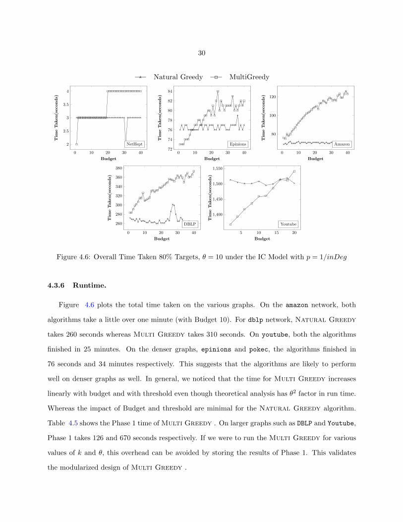
Figure 4.6 plots the total time taken on the various graphs. On the amazon network, both

algorithms take a little over one minute (with Budget 10). For dblp network, Natural Greedy

takes 260 seconds whereas Multi Greedy takes 310 seconds. On youtube, both the algorithms

finished in 25 minutes. On the denser graphs, epinions and pokec, the algorithms finished in

76 seconds and 34 minutes respectively. This suggests that the algorithms are likely to perform

well on denser graphs as well. In general, we noticed that the time for Multi Greedy increases

linearly with budget and with threshold even though theoretical analysis has θ2 factor in run time.

Whereas the impact of Budget and threshold are minimal for the Natural Greedy algorithm.

Table 4.5 shows the Phase 1 time of Multi Greedy . On larger graphs such as DBLP and Youtube,

Phase 1 takes 126 and 670 seconds respectively. If we were to run the Multi Greedy for various

values of k and θ, this overhead can be avoided by storing the results of Phase 1. This validates

the modularized design of Multi Greedy .

31

CHAPTER 5. SUMMARY AND FUTURE WORK

5.1 Summary

In this thesis, we studied the Constrained Influence Maximization (CIM ) problem. The objec-

tive is to influence Target users with the hard constraint on the number of adversarial Non-Target

users influenced. Despite the theoretical hardness of CIM , we’ve provided efficient RIS based

designs of Natural Greedy and Multi Greedy algorithms.

5.2 Future Work

In CIM , the number of adversaries or Non Targets is limited by a hard constraint. The

question then arises: Are there scenarios where this hard constraint must be relaxed? The choice

for threshold θ will vary based on the size of the graph, the application, etc. Consider a political

ad campaign: The objective can be to spread the ad maximally, while still influencing a minimal

number of non-targets. One could tolerate higher numbers of Non-Targets influenced provided more

Targets are also influenced (with the motivation still being to minimize Non-Targets influenced).

We can view this problem as the maximizing difference of the number of Targets and Non-Targets.

Problem 3. Given a network G = (V,E) and k, compute S ⊆ V , |S| = k such that h(S) =

σT (S)− σN (S) is maximized.

While the problem of maximizing the difference between two submodular functions has been

studied [21, 11], there are two major unexplored areas. Firstly, unlike Problem 3, there is no

cardinality constraints in the existing literature. Secondly, the existing algorithms are designed for

general submodular functions and not the influence function under the IC/LT models. We plan to

study Problem 3 as the next step in understanding how to maximize influence in the presence of

Non-Targets.

32

REFERENCES

[1] C. Aslay, N. Barbieri, F. Bonchi, and R. Baeza-Yates. Online topic-aware influence maximiza-

tion queries. In Proc. of the 17th EDBT 2014., pages 295–306, 2014.

[2] C. Borgs, M. Brautbar, J. Chayes, and B. Lucier. Maximizing social influence in nearly optimal

time. In Proc. of the 25th SODA 2014, pages 946–957, 2014.

[3] S. Chen, J. Fan, G. Li, J. Feng, K-L. Tan, and J. Tang. Online topic-aware influence maxi-

mization. Proc. VLDB Endow., 8(6):666–677, 2015.

[4] W. Chen, C. Wang, and Y. Wang. Scalable influence maximization for prevalent viral mar-

keting in large-scale social networks. In KDD, pages 1029–1038, 2010.

[5] W. Chen, Y. Wang, and S. Yang. Efficient influence maximization in social networks. In KDD,

pages 199–208, 2009.

[6] W. Chen, Y. Yuan, and L. Zhang. Scalable influence maximization in social networks under

the linear threshold model. In ICDM, pages 88–97, 2010.

[7] X. Fu, M.R. Padmanabhan, R.G. Kumar, S. Basu, S. Dorius, and A. Pavan. Measuring the

impact of influence on individuals: Roadmap to quantifying attitude. https://arxiv.org/

abs/2010.13304, 2020.

[8] X. Fu, M.R. Padmanabhan, R.G. Kumar, S. Basu, S. Dorius, and A. Pavan. Measuring

the impact of influence on individuals: Roadmap to quantifying attitude. In Proceedings of

the 2020 IEEE/ACM International Conference on Advances in Social Networks Analysis and

Mining, ASONAM ’20 (in press). Association for Computing Machinery, 2020.

[9] A. Goyal, W. Lu, and L. Lakshmanan. Celf++: Optimizing the greedy algorithm for influence

maximization in social networks. In WWW, pages 47–48. ACM, 2011.

33

[10] J. Guo, P. Zhang, C. Zhou, Y. Cao, and L. Guo. Personalized influence maximization on social

networks. In Proc. of CIKM 13, pages 199–208, 2013.

[11] Rishabh K. Iyer and Jeff A. Bilmes. Algorithms for approximate minimization of the difference

between submodular functions, with applications. CoRR, abs/1207.0560, 2012.

[12] Rishabh K. Iyer and Jeff A. Bilmes. Submodular optimization with submodular cover and

submodular knapsack constraints. CoRR, abs/1311.2106, 2013.

[13] K. Jung, W. Heo, and W. Chen. IRIE: scalable and robust influence maximization in social

networks. In 12th ICDM 2012., pages 918–923, 2012.

[14] D. Kempe, J. Kleinberg, and E. Tardos. Maximizing the spread of influence through a social

network. In KDD, pages 137–146, 2003.

[15] Elias Boutros Khalil, Bistra Dilkina, and Le Song. Scalable diffusion-aware optimization of

network topology. In Proceedings of the 20th ACM SIGKDD International Conference on

Knowledge Discovery and Data Mining, KDD ’14, page 1226–1235, New York, NY, USA,

2014. Association for Computing Machinery.

[16] Raj Gaurav Kumar, Preethi Bhardwaj, S. Basu, and A. Pavan. Disrupting diffusion: Critical

nodes in network. In IEEE/ACM/WIC Joint Conference on Web Intelligence and Intelligent

Agent Technology, To Appear, 2020.

[17] J-R. Lee and C-W. Chung. A query approach for influence maximization on specific users in

social networks. IEEE Trans. Knowl. Data Eng., 27(2):340–353, 2015.

[18] Jure Leskovec, Andreas Krause, Carlos Guestrin, Christos Faloutsos, Jeanne VanBriesen, and

Natalie Glance. Cost-effective outbreak detection in networks. In Proceedings of the 13th ACM

SIGKDD International Conference on Knowledge Discovery and Data Mining, KDD ’07, pages

420–429, New York, NY, USA, 2007. ACM.

34

[19] F.H. Li, C.T. Li, and M.K. Shan. Labeled influence maximization in social networks for target

marketing. In PASSAT/SocialCom 2011, pages 560–563, 2011.

[20] Y. Li, D. Zhang, and K-L. Tan. Real-time targeted influence maximization for online adver-

tisements. VLDB, 8(10):1070–1081, 2015.

[21] M. Narasimhan and J. Bilmes. A submodular-supermodular procedure with applications to

discriminative structure learning. In (UAI), pages 404–412, 2005.

[22] G. L. Nemhauser, L. A. Wolsey, and M. L. Fisher. An analysis of approximations for maxi-

mizing submodular set functions—i. Mathematical Programming, 14(1):265–294, Dec 1978.

[23] Hung T. Nguyen, My T. Thai, and Thang N. Dinh. Stop-and-stare: Optimal sampling algo-

rithms for viral marketing in billion-scale networks. CoRR, abs/1605.07990, 2016.

[24] N. Ohsaka, T. Akiba, Y. Yoshida, and K. I. Kawarabayashi. Fast and accurate influence

maximization on large networks with pruned monte-carlo simulations. In Proceedings of the

AAAI, pages 138–144, 2014.

[25] M. R. Padmanabhan, N. Somisetty, S. Basu, and A. Pavan. Influence maximization in social

networks with non-target constraints. In 2018 IEEE International Conference on Big Data

(Big Data), pages 771–780, 2018.

[26] Ramakumar Pasumarthi, Ramasuri Narayanam, and Balaraman Ravindran. Near optimal

strategies for targeted marketing in social networks. In AAMAS, pages 1679–1680, 2015.

[27] Naresh Somisetty. Targeted influence maximization in labeled social networks with non-target

constraints. Master’s thesis, Iowa State University, 2017.

[28] C. Song, W. Hsu, and M. L. Lee. Targeted influence maximization in social networks. In Proc.

of CIKM 16, pages 1683–1692, 2016.

[29] Y. Tang, Y. Shi, and X. Xiao. Influence maximization in near-linear time: A martingale

approach. In SIGMOD, pages 1539–1554, 2015.

35

[30] Y. Tang, X. Xiao, and Y. Shi. Influence maximization: near-optimal time complexity meets

practical efficiency. In SIGMOD, pages 75–86, 2014.

[31] Y. Wang Y. Li, J. Fan and K. Tan. Influence maximization on social graphs: A survey. vol.

30:1852–1872, 2018.