1

Spread-F occurrence during geomagnetic storms near the southern crest

of the EIA in Argentina

Gilda de Lourdes González1,2

1Universidad Nacional de Tucumán (UNT)

Av. Independencia 1800 – San Miguel de Tucumán (4000) – Argentina 2Universidad del Norte “Santo Tomás de Aquino” (UNSTA)

9 de Julio 165, T4000 San Miguel de Tucumán, Tucumán

gilda.gonzalez@unsta.edu.ar

(Accepted for publication in ASR October, 30 2020)

------------------------------------------------------------------------------------------- ---------------------------------------------------------------

Abstract This work presents, for the first time, the analysis of the occurrence of ionospheric

irregularities during geomagnetic storms at Tucumán – Argentina, a low latitude station in the

Southern American longitudinal sector ( 26.9 ° S, 294.6 ° E; magnetic latitude 15.5 ° S), near the

southern crest of the equatorial ionization anomaly (EIA). Three geomagnetic storms occurred

on May 27, 2017 (a month of low occurrence rates of spread-F), October 12, 2016 (a month of

transition from low to high occurrence rates of spread-F) and November 7, 2017 (a month of

high occurrence rates of spread-F) are analyzed using Global Positioning System (GPS) receivers

and ionosondes. The rate of change of total electron content (TEC) Index (ROTI), GPS Ionospheric

L-band scintillation, the virtual height of the F-layer bottom side (h'F) and the critical frequency

of the F2 layer (foF2) are considered. Furthermore, each ionogram is manually examined for the

presence of spread-F signatures.

The results show that, for the three events studied, geomagnetic activity creates favorable

conditions for the initiation of ionospheric irregularities, manifested by ionogram spread-F and

TEC fluctuation. Post-midnight irregularities may have occurred due to the presence of eastward

disturbance dynamo electric fields (DDEF). For the May storm, an eastward over-shielding

prompt penetration electric field (PPEF) is also acting. A possibility is that the PPEF is added to

the DDEF and produces the uplifting of the F region that helps trigger the irregularities. Finally,

during October and November, strong GPS L band scintillation is observed associated with

strong range spread-F (SSF), that is, irregularities extending from the bottom-side to the topside

of the F region.

Keywords: Low Latitude Ionosphere; Spread-F; Geomagnetic storm; space weather

------------------------------------------------------------------------------------------------------------------------------

1. Introduction

The response of the low-latitude

ionosphere to geomagnetic storms is a

prominent topic of study in space weather.

There is significant interest in describing the

short-term variability of the ionosphere and

developing prediction models for

ionospheric weather.

The ionospheric irregularities occurrence

pattern can be modified drastically during

magnetic storms and it may affect the GNSS

and VHF signals, so the analysis of the

occurrence of irregularities during

geomagnetic storms has important

applications in navigation and positioning

systems, as well as in trans-ionospheric

communications.

In this work the ring current Dst index is

used to classify the geomagnetic storms

(Gonzalez, Tsurutani, & Clúa De Gonzalez,

1999). If the minimum Dst is < -100 nT the storm is intense, -100 nT ≤ Dst < -50 nT

corresponds to a moderate storm and -50

nT ≤ Dst < -30 nT characterize a weak storm.

2

The Dst index is based on the depression in

the H component of the geomagnetic field

at low latitudes caused by an enhancement

in the ring current during the storm.

Low-latitude electric fields can be

significantly disturbed during storms. Two

main high-latitude sources of these changes

are: The solar wind-magnetosphere

dynamo and the ionospheric disturbance

dynamo. The first one generates rapid and

short-lived (2–3 h) (prompt) electric field

perturbations associated with rapid

changes in the polar cap potential (Senior

and Blanc, 1984). When the polar cap

potential increases suddenly the situation is

called “under-shielding”, and the associated

electric field (PPEF) has eastward polarity

during the day and westward polarity after

~22LT. On the other hand, an over-shielding

electric field (PEF) is associated with the

recovery of the polar cap potential and has

its polarity opposite to that of the PPEF. The

ionospheric disturbance dynamo results

from thermospheric disturbance winds

generated by Joule heating at auroral

latitudes during periods of high magnetic

activity (Blanc and Richmond, 1980). It

produces disturbance wind dynamo electric

fields (DDEF) that could last several hours

and has a polarity local time dependence

that is opposite to that of the PEF. The DDEF

is delayed by a few hours with respect to the

storm onset (M. a. Abdu, 2012; B. G. Fejer,

Larsen, & Farley, 1983; Bela G. Fejer,

Jensen, & Su, 2008).

The ionospheric instabilities in F region are

grouped under the name of Spread-F. This

term was coined to describe the effect of

broadening in frequency (frequency spread-

F, FSF) and / or in range (range spread-F,

RSF) observed in echo traces of ionograms.

This is due to multiple reflection paths

created by the turbulent ionosphere when

there is a process of instability above the

ionosonde. Spread-F extends from the F

region to 1700 km, and is a nighttime

phenomenon. During quiet geomagnetic

conditions it occurs mainly before midnight

(M A Abdu, de Medeiros, Sobral, &

Bittencourt, 1982; Calvert, 1962; Piggott &

Rawer, 1972). RSF is associated with the

development of plasma bubbles (PB) (Abdu

et al., 2003), regions of very low plasma

density and a high electric field. These

plasma irregularities develop through the

Rayleigh-Taylor instability (RTI) process,

which operates at the bottom side of the F-

region. In the South American longitude

sector there are distinct RSF/PB seasons,

with high occurrence of RSF during the

December solstice months (November to

February) and low occurrence during the

June solstice months (May to August), while

the equinox months (March, April,

September and October) presents

transition characteristics from high to low

occurrence and vice versa.

Figure 1. Map showing the location of Tucumán (blue circle).

3

There has been several attempts to find a

correlation between the geomagnetic

activity and the occurrence of RSF/PB at low

latitudes (M. A. Abdu et al., 2012;

Jayachandran, Ram, Somayajulu, & Rao,

1997; Martinis, 2005; Pavlov et al., 2006;

Ray, Roy, & Das, 2015, and references

therein). Earlier studies show that the RSF is

reduced during disturbed geomagnetic

conditions (Lyon, Skinner, & Wright, 1960).

More recent works conclude that at low

latitudes during the low equatorial plasma

bubbles occurrence season and transition

season, geomagnetic activity helps in the

generation process of PB, whereas during

the high PB season it acts as inhibitor

(Becker-Guedes et al., 2004). Some authors

have reported the occurrence of post-

sunset RSF during the main phase of a

geomagnetic storm for periods of low

occurrence rates of spread-F. Basu et al.

(2001) analyzed the augmentation or

inhibition of spread-F during two major

geomagnetic storms for low and middle

latitudes. They concluded that PPEF

generate post-sunset spread-F at low

latitudes and coincides with an increased in

AE index and a decrease in SYM-H index.

They also showed that the time variation of

the SYM-H is an indicator for the time of

prompt penetration. Other studies

concluded that, depending on the phase of

the storm, geomagnetic activity can either

suppress or trigger the generation of

spread-F in the post-sunset period (pre-

midnight). A consensus is that the

probability of spread-F occurrence during

the post-midnight period increases with

geomagnetic activity (Bowman, 1991;

Sobral et al., 1997).

This work reports for the first time the

influence of three geomagnetic storms on

the occurrence of RSF/PB in Tucuman—

Argentina. Data from ionosonde and Global

Positioning System (GPS) are used. The

geomagnetic storms occurred on 2016 and

2017, at the end of the descending phase of

the 24th solar cycle. The chosen seasons are

winter and summer of 2017 (May and

November) and equinox of 2016 (October).

Two of these storms, the one occurred in

May and the one occurred in October are

caused by a coronal mass ejection (CME)

whereas the storm occurred in November is

caused by a high-speed solar wind stream

(HSSWS).

2. Data and methodology

The different phases of a geomagnetic

storm (initial, main and recovery) are

determined by the variation in Dst

geomagnetic index. This index is obtained

from the World Data Center (WDC) Kyoto,

Japan website http://wdc.kugi.kyoto-

u.ac.jp/dstae/ index.html. The north-south

component of the interplanetary magnetic

field (IMF_Bz) obtained from the Advanced

Composition Explorer (ACE) and the dawn-

to-dusk interplanetary electric field (IEF_Ey)

are analyzed. Additionally, Kp (a 3-hourly

planetary index of geomagnetic activity)

and AE (a geomagnetic index of the auroral

electrojet) are taken from the NASA’s Space

Physics Data Facility (NASA, Goddard Space

Flight Center,

https://omniweb.gsfc.nasa.gov). The

ionospheric sounding data is obtained by

two ionosondes: The Advanced Ionospheric

Sounder (AIS) and the Vertical Incidence

Pulsed Ionospheric Radar (VIPIR). Both

instruments are located in Tucumán (26.9 °

S, 294.6 ° E, lat. Geomagnetic 15.5 S). Figure

1 shows the geographic location of the

analyzed region. The sweeping frequency of

the AIS ionosonde is from 1 to 20 MHz and

the sounding repetition rate is 10 minutes,

the ionograms are available at the

electronic Space Weather upper

atmosphere database (eSWua)

(http://www.eswua.ingv.it/). The VIPIR

operates between 0.3 and 25 MHz with a

sounding repetition rate of 5 minutes

(Bullett, 2008), the ionograms can be

obtained from the website of the Low

Latitude Ionospheric Sensor Network (LISN)

4

(http://lisn.igp.gob.pe). Each ionogram is

manually examined for the presence of RSF.

Also, the virtual height of the F-layer bottom

side, h'F and the critical frequency of the F2-

layer, foF2, are extracted. For the AIS

ionosonde, the parameters are auto scaled

by the Autoscala system (Pezzopane and

Scotto 2005) and for the VIPIR ionosonde,

the parameters are manually scaled.

The Total Electron Content (TEC) is obtained

from a GPS ground-based receiver located

at Tucuman, and the raw GPS observables

are available at the Argentine Continuous

Satellite Monitoring Network (RAMSAC)

website

(http://www.ign.gob.ar/NuestrasActividad

es/Geodesia/Ramsac) (Piñón et al.,

2018).The slant TEC along the satellite-

receiver line of sight is estimated with the

GPS-TEC calibration technique developed

by Dr. Krishna Seemala Gopi of the Indian

Institute of Geomagnetism (IIG), Navi

Mumbai, India (GPS_Gopi_v2.9.5:). An

elevation mask of 25° has been applied to

reduce the effects of multipath.

Ionospheric storms have been categorized

by as positive and negative phases. A

positive phase results in increased electron

density from the quiet time values.

Whereas a negative phase results in

decreased electron density from the quiet

time values. The response of the

ionospheric F-region to a geomagnetic

storm is analyzed using ΔTEC, that is the

deviations of TEC from the reference,

expressed in Eq. 1. Therefore, ΔTEC > 0

indicates a positive phase and ΔTEC < 0

indicates a negative phase.

𝛥𝑇𝐸𝐶 =𝑇𝐸𝐶̅̅ ̅̅̅̅ −⟨𝑇𝐸𝐶̅̅ ̅̅̅̅ ⟩

⟨𝑇𝐸𝐶̅̅ ̅̅̅̅ ⟩× 100 (1)

𝑇𝐸𝐶̅̅ ̅̅̅̅ is the mean TEC considering all the

visible satellites during a day, ⟨𝑇𝐸𝐶̅̅ ̅̅̅̅ ⟩ is the

average 𝑇𝐸𝐶̅̅ ̅̅̅̅ calculated using the ten International Quietest Days (IQDs) of the

month. IQDs are derived from GFZ-Potsdam

(https://www.gfz-potsdam.de/en/kp-

index/).

Ionospheric L-band scintillation is also

obtained from the GPS receiver.

Scintillation index S4 is used to quantified

the strength of the amplitude scintillation.

S4 > 0.5 indicates strong scintillation and 0.1

< S4 ≤ 0.5 indicates weak scintillation

activity (Davies, 1990). The S4 data is

obtained from the LISN database for May

and October and from the GPS Ionospheric

Scintillation receiver owned by Istituto

Nazionale di Geofisica e Vulcanologia

(INGV) for November.

Furthermore, the rate of change of TEC

(ROT) along the signal path from each

visible satellite to the receiver and the rate

of TEC index (ROTI) are computed. The ROT

and ROTI can be used to detect the

presence of GPS ionospheric irregularities

during magnetic storms (Pi et al., 1997; Basu

et al., 1999; Azzouzi et al., 2016; Dugassa,

Habarulema, & Nigussie, 2020). The ROT is

the rate of change of slant TEC (Eq. 2) and

the ROTI is defined as the standard

deviation of ROT (Eq. 3).

𝑅𝑂𝑇 =TEC𝑘

𝑖 −TEC𝑘−1𝑖

𝑡𝑘−𝑡𝑘−1 (2)

𝑅𝑂𝑇𝐼 = √⟨𝑅𝑂𝑇2⟩ − ⟨𝑅𝑂𝑇⟩2 (3)

Where k is the time of epoch and i is the

visible satellite. In the present work, the

sampling interval used to calculate ROT is

0.5 min and the time window of the

standard deviation of ROTI is 5 min.

ROTI is divided into different levels, ROTI <

0.25 indicates no TEC fluctuations, 0.25 ≤

ROTI < 0.5 are considered weak TEC

fluctuations, 0.5 ≤ ROTI < 1 signifies

moderate TEC fluctuations and ROTI ≥ 1 are

strong TEC fluctuations (Atıcı & Sağır, 2019;

Liu, Yuan, Tan, & Li, 2016; Ma & Maruyama,

2006).

3. Results

3.1. The Storm of May 27, 2017

5

The storm occurred in May, a month of low

occurrence rates of spread – F, with a

monthly mean F10.7 flux of 76.3 solar flux

unit (sfu). The storm reaches a minimum Dst

of -125 nT, and a Kp of 7, which makes it is

an intense storm. It is produced by a CME

released by the sun on May 23, 2017, that

arrived at earth four days later. The sudden

storm commencement (SSC) occurs at 15:34

UT (12:34 LT) on May 27

(http://www.obsebre.es/en/rapid), the

initial phase lasts until 19 UT (16 LT) and the

main phase is maintained until May 28 at 7

UT (4 LT) when the Dst index reaches the

minimum. Figure 2 shows the IMF_Bz

obtained from ACE and the interplanetary

electric field IEF_Ey as a function of the

universal time UT (LT = UT – 3). The

geomagnetic indices Dst, Kp and AE, and the

ionospheric parameters h´F and foF2 scaled

from the ionograms are also plotted in the

same figure. The periods with RSF are

highlighted with vertical bars.

It is observed that Bz presents a strong

southward excursion during the storm main

phase, between 20 UT (17 LT) on May 27

and 15 UT (12 LT) on May 28, with a

minimum of -19.5nT at 0 UT on the same

day (21 LT May 27), then it turns northward

and remain thus during about 19 hours with

a peak of 11.6 nT at 22 UT on May 28. The

interconnection between the IMF and the

Earth´s magnetic field is produced during

the southward Bz period and results in the

large decrease observed in Dst. Ey shows a

large increase during the main phase and

has a maximum of 7.72 mV/m at 23 UT (20

LT) on May 27. The AE index (which is a

measure of currents in the auroral

electrojet) shows a small peak of 361 nT at

16 UT (13 LT) on May 27, during the initial

phase of the storm. It then increases from

34 nT to 943 nT between 20 – 23 UT (17 –

20 LT). Small-amplitude fluctuation can be

seen at 23 – 5 UT (20 – 2 LT) on May 28

(storm main phase) with a peak of 1271nT.

Finally, AE decreases to quiet values during

the recovery phase of the storm. The foF2

data shows an increase of 1.7MHz during

the initial phase of the storm compared to

the quiet-time levels (overage of the 10

IQDs of May 2017) with a peak of 8.3 MHz

at 18 UT (15 LT) on May 27. A larger

intensification of about 4.5 MHz occurs

during the recovery phase, with a peak of

10.3 MHz at 16 UT (13 LT) on May 28. The

bottom panel shows the variation of h´F, it

is observed that during the initial phase h´F

is close to its quiet-time reference value,

then on May 28, h´F increases from ~213 km

to 357 km at 0 – 4 UT (21 – 1 LT), it increased

54% more than the quiet time curve in the

same period. This behavior coincides with

the large sudden increase in the AE index

during the second half of the main phase.

Finally, during the recovery phase, h'F

decreases irregularly to quiet levels.

To study the Earth´s electric field

penetration, ΔH is used to infer the electric

field at low latitudes. ΔH is the difference in

the magnitudes of the horizontal

geomagnetic field component (H) between

a magnetometer placed on the magnetic

equator and one displaced 6°- 9° away. As it

is explained by Wei et al. (2015), ΔH is

related to the equatorial electrojet (EEJ) and

the EEJ is linearly related to the electric

field. Figure 3 shows the difference

between H at Jicamarca (dip latitude 0.4°N)

and Piura (dip latitude 6.8°N), Peru. A weak

positive perturbation of ΔH is observed on

May 28 at 3 – 8 UT (0 – 5 LT), that

corresponds to an eastward electric field

likely associated to Bz slowly turning north.

Figure 4 shows the day-to-day variability of

RSF over Tucuman during May 2017,

observed with the ionosonde AIS. The y-axis

represents the day of the month and the x-

axis represents the hour (UT) of the day. The

graphic shows that RSF is present in four

days: the three most disturbed days of May

(28, 20 and 19) and one quiet day (May 5) at

1 – 4:30 LT. During the period of the storm,

the ionograms show RSF during the second

6

Figure 2. Kp index, Dst, Bz, Ey, AE, foF2 and h´F for Tucumán

during May 27 – 29, 2017. The shaded region indicates the

occurrence of RSF.

Figure 3. Time variations of Dst (nT), Bz (nT), AE (nT) and difference

between horizontal geomagnetic field components (H) at Jicamarca

and Piura, Peru, during May 27 – 29, 2017. The shaded region

indicates the occurrence of RSF.

Figure 4. Day-to-day variability of RSF occurrence over Tucuman during May 2017, RSF (red).

7

part of the main phase, in the interval 01:40

UT – 07:40 UT (May 27 22:40 LT – May 28

04:40 LT). During the disturbed period, RSF

appears before local midnight and it is more

intense. To see the evolution of the spread-

F on May 28 at Tucuman, figure 5 illustrates

the beginning, evolution process, and end

of the irregularities.

Figure 6 shows the TEC estimated from a

GPS receiver at Tucuman from different

satellites, it is possible to see TEC depletions

on May 28 at ~1 – 7 UT (22 – 4 LT) for most

of the satellites in view. In order to analyze

this data segment more deeply, the TEC

perturbations (TECp) along PRNs 12 and 15

arcs are calculated according to Eq. (4).

𝑇𝐸𝐶𝑝𝑖 (𝑡) = 𝑇𝐸𝐶𝑖(𝑡) − ⟨𝑇𝐸𝐶𝑖(𝑡)⟩ (4)

Where 𝑇𝐸𝐶 𝑖(𝑡) is the TEC value along the

satellite i and the receiver at a time t and

⟨𝑇𝐸𝐶 𝑖(𝑡)⟩ is the corresponding 1 h running

mean.

Fast Fourier Transform (FFT) analysis

(periodogram) is performed on the data to

identify different periods. Figure 7 shows

the FFT of TEC perturbations characterizing

PRNs 12 and 15 on May 28 2017 from 1 UT

to 7 UT. It is observed that dominant

periods of ~70 and ~ 40 minutes are present

in both cases. These TEC depletions could

be due to the propagation of Atmospheric

Gravity Waves (AGW) in the ionospheric F

region that generate traveling ionospheric

disturbances (TIDs) (Hines, 1959; Hooke,

1968; Hunsucker, 1982; Kirchengast et al.,

1996; Valladares et al., 2009) .

Figure 8a and b shows variations of VTEC,

ROT index and ROTI index over Tucumán for

PRN 12 and 15 during May 27-29, 2017. As

it was mentioned before, TEC profile for

both PRNs is characterized by depletions on

May 28, while it is smooth on May 27 and

29. On May 28 between 1 – 4 UT, for PRN 12

and 15, ROT level is ~ 1 TECU/min and ROTI

presents values of 0.5 – 1 TECU/min, this

indicates moderate TEC fluctuations.

The analysis of the scintillation index S4

(figure 9) for the period of the storms

reveals a weak scintillation activity given

that S4 is always between 0.1 and 0.3. Thus,

the electron density irregularities

associated with the PB observed in the

period of the storm do not cause significant

amplitude scintillation.

Figure 10 shows the deviation, 𝛥𝑇𝐸𝐶, for

May 27 – 29, 2017 calculated with Eq. (1).

The data presents an irregular behavior

with small effects during the initial and the

first part of the main phase; first a negative

ionospheric storm phase is present on May

27 between 15:30 UT and 17:30UT (12:30 LT

– 14:30 LT) followed by a short-lived

positive phase between 17:30 UT – 19 UT

(14:30 LT – 16 LT) and then a negative phase

again from May 27 at 19 UT (16 LT) to May

28 at 23:30 UT (20:30 LT). During the last

part of the main phase, a positive

ionospheric storm effect is observed on

May 28 between 23:30 UT and 6 UT (20:30

LT – 3 LT) with a peak of 96% at 2 UT on May

28 (May 27, 23 LT) followed by minor

negative disturbances during the first part

of the recovery phase on May 28 between 6

UT and 10 UT (3 LT – 7 LT). A positive storm

is observed on May 28 between 10 UT (7 LT)

and 22 UT (19 LT), positive values of ΔTEC

exceed 100% and the peak enhancement

occurs almost 7 hours after the minimum

Dst. Finally, an irregular behavior is

observed during the recovery phase, with

minor positive and negative disturbances.

3.2. The Storm of October 12, 2016

A CME that hit our planet on October 12 (a

month of transition from low to high

occurrence rates of spread-F) at 22:12 UT

(19:12 LT) caused a geomagnetic storm with

a minimum Dst of -104 nT. For this month

the mean F10.7 index is 84.6 sfu. Figure 11

shows the geomagnetic indices and the F-

layer parameters foF2 and h’F during

October 12 – 14, 2016. The main phase of

the storm starts at 6 UT (3 LT) on October 13

8

Figure 5. Ionograms recorded at Tucuman showing the presence of RSF on May 28, 2017.

Figure 6. TEC calibrated from a GPS receiver at Tucuman. TEC depletions

are indicated with a black circle on May 28 at ~1 – 7 UT (22 – 4 LT).

Figure 7. Upper panel, the TEC perturbations characterizing PRNs 12 (left) and 15 (right) on May 28, 2017. Bottom panel, FFT of TEC perturbations characterizing PRNs 12 (left) and 15

(right).

9

Figure 8a. Variations of VTEC, ROT and ROTI for PRN 12 over Tucumán during May 27 – 29, 2017.

Figure 8b. Variations of VTEC, ROT and ROTI for PRN 15 over Tucumán during May 27 – 29, 2017.

10

Figure 9. The temporal variation of Global Positioning

System L-band scintillation over Tucuman on May 27, 28

and 29 2017.

Figure 10. Deviation ΔTEC between the TEC values for May 27- 29, 2017 and the average TEC of the 10 quietest

days of May 2017.The shaded region indicates the period when spread -F is observed in ionograms.

11

and remains until 17 UT (14 LT) followed by

a gradual recovery. The highest Kp is 6 and

occurs at 15 UT (12 LT) on October 13. AE

and Ey show a rapid increase coinciding with

an intense Bz south condition from October

13 at 6 UT (3 LT) till October 14 at 9 UT (6

LT), Bz has a minimum value of -20.8 nT at

16 UT (13 LT) on October 13, AE has a

maximum value of 1200 nT at 15 UT (12 LT)

while the highest value of Esw is 16 mV/m at

16 UT (13 LT). During the recovery phase of

the storm, Bz turns north while AE and E

decrease to quiet values.

It is observed that during the period of the

storm, foF2 is generally higher than the

quiet values (overage of the 10 IQDs of

October 2016), specially between 18 UT (15

LT) and 6 UT (3 LT). The largest difference is

4.5 MHz and occurs at 2 UT on October 13

(23 LT October 12), during the initial phase

of the storm. The peak value of foF2 is 16.6

MHz at 22 UT (19 LT) on October 13.

As for h’F, it is observed that the disturbed

values are usually higher than the quiet

ones, except during the initial phase when

the values for both periods are similar.

During the recovery phase on October 14,

h’F increases from ~216 km to ~336 km at 1

– 4 UT (22 – 1 LT), ~38% more than the quiet

value and during the main phase, on

October 13 around 15 UT (12 LT) h’F is ~22%

higher than for quiet days. There is no data

for h´F and foF2 for the periods with RSF as

it is observed in the curves of figure 7.

Time variations of ΔH for October 12-14 are

shown in figure 12. A negative perturbation

is observed on October 13 at 9-13 UT (6-10

LT) that can be associated with a westward

electric field. ΔH does not present

perturbations during the periods with

ionospheric irregularities.

Figure 13 illustrates the day-to-day

variability of RSF over Tucumán during

October 2016. RSF is present in six days:

three of the most disturbed days of the

month (25, 13 and 29) and one of the ten

quietest days (October 19) between 2 – 6 UT

(23 – 3 LT), except on October 14 and

October 29 when RSF is also observed after

6 UT. During the period of the storm,

spread-F is observed during the initial

phase, on October 13 at 3:30 – 4:20 UT (0:30

– 1:20 LT), and during the recovery phase on

October 14 at 8:50 – 11:50 UT (5:50 – 8:50

LT), indicated with gray bars in figure 12.

Two of these ionograms are shown in figure

14. It is observed that in these periods the

range spread on F layer echo extends to

higher frequencies (~15 MHz), beyond the

local foF2 value (~11 MHz), than that

present during the storm of May 27 (~8

MHz). This type of spread-F is often called

Strong range Spread-F (SSF) and considered

as an independent type of spread-F.

TEC depletions are observed on October 13

and 14 in coincidence with the presence of

RSF in ionograms as is shown in figure 15. In

the same way as in the previous storm,

periodogram analysis is performed in the

TECp to identify different periods. PRN 1

and 27 are considered, the periods found

are ~ 48 and 34 minutes (see figure 16).

On October 13 between 2-3 UT, VTEC

depletions are present in PRN 27, ROT levels

are ~ 1 TECU/min and ROTI values are 0.6 –

0.8 TECU/min (fig. 17a). On October 14, PRN

1 shows TEC depletions between 9-10 UT,

ROT levels are ~3TECU/min and ROTI is 1.2

– 1.8 TECU/min, this indicates strong TEC

fluctuations (fig. 17b).

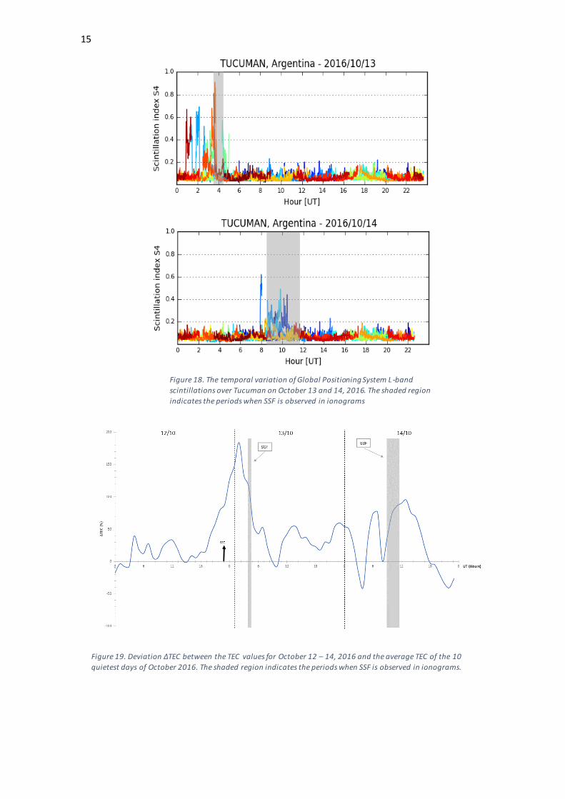
Figure 18 shows the temporal variation of

the scintillation index S4 over Tucuman on

October 13 and 14, 2016. Strong

scintillation (i.e., S4 ≥ 0.5) is observed on

October 13 at 1 – 5 UT (22 – 3 LT) and on

October 14 around 10 UT (7 LT). Ionograms

SSF and GPS – TEC fluctuations occur almost

simultaneously with high amplitudes of S4.

Likely the strong scintillation activity could

be associated with the field-aligned

irregularities (FAIs) with a spatial scale of a

few hundred meters that are confined

12

Figure 11. Kp index, Dst, Bz, Ey, AE, foF2 and h´F for Tucumán

during October 12 – 14, 2016. The shaded regions denote the

periods with spread-F.

Figure 12. Time variations of Dst (nT), Bz (nT), AE (nT) and

difference between horizontal geomagnetic field components (H) at Jicamarca and Piura, Peru, during October 12 – 14, 2016. The

shaded regions denote the periods with spread-F.

Figure 13. Day-to-day variability of RSF occurrence over Tucuman during October 2016, RSF (red).

13

Figure 14. Sample of strong spread-F (SSF) observed in ionograms recorded using the AIS ionosonde at Tucuman –

Argentina on October 13 (left) and 14 (right), 2016.

Figure 15. TEC calibrated from a GPS receiver at Tucuman. TEC depletions (indicated with a black

circle) are observed on October 13 at ~3 – 5 UT (0 – 2 LT) and on October 14 at ~8 – 11 UT (5 – 8 LT).

Figure 16. Upper panel, the TEC perturbations characterizing PRN 27 on October 13, 2016 (left) and

PRN 1 on October 14 (right). Bottom panel, FFT of TEC perturbations characterizing PRN 27 (left)

and PRN 1 (right).

14

Figure 17a. Variations of VTEC, ROT and ROTI for PRN 27 over Tucumán during October 12 – 14, 2016.

Figure 17b. Variations of VTEC, ROT and ROTI for PRN 1 over Tucumán during October 12 – 14, 2016.

15

Figure 18. The temporal variation of Global Positioning System L -band

scintillations over Tucuman on October 13 and 14, 2016. The shaded region

indicates the periods when SSF is observed in ionograms

Figure 19. Deviation ΔTEC between the TEC values for October 12 – 14, 2016 and the average TEC of the 10

quietest days of October 2016. The shaded region indicates the periods when SSF is observed in ionograms.

16

within the PBs (Otsuka, Shiokawa and

Ogawa, 2006).

𝛥𝑇𝐸𝐶 vs UT is shown in figure 19 for

October 12 – 14. The dominant feature is

the absence of significant negative

disturbances and the presence of a large

positive effect during the initial phase of the

storm with a peak of 184% at 2 UT on

October 13 (23 LT October 12). On October

14, 3 – 5 UT (0 – 2 LT) a negative effect is

observed, with a peak of -39.7% at 4 UT (1

LT) on October 14.

3.3. The Storm of November 7, 2017

A moderate geomagnetic storm occurs on

November 7, 2017 (a month of high

occurrence rates of spread-F) caused by the

impact of high-speed solar wind streams

(HSSWS) emanated from a solar coronal

hole, with speeds near 650 km/s. The fast

streams interact with the slow streams

forming and interface region known as Co

rotating Interaction Region (CIR). An

important aspect of the CIRs is the presence

of Alfvén waves in the magnetic field.

During this month the mean F10.7 is 70.3

sfu and the Kp reaches a maximum of 6.3 on

November 7 at 18 UT (15 LT) and on

November 8 at 3 UT (0 LT). A gradual initial

phase (not a sudden commencement) starts

on November 7 at ~1 UT (November 6, 22

LT) and finished at about 8 UT (5 LT). The

main phase lasts until November 8 at 1 UT

(November 7, 22 LT) when the Dst reaches

its minimum value of -72 nT. After that, a

long recovery phase is observed, IMF Bz

oscillations diminish but intense auroral

activity is still present with AE values higher

than 1000 nT on November 8. This is not a

High-Intensity, Long-Duration, Continuous

AE Activity, or HILDCAA event since the

active conditions last less than two days

(Tsurutani & Gonzalez, 1987).

The response of the F-region over Tucuman

during this geomagnetic storm is presented

in Figure 20. During the period of analysis

IMF Bz is highly variable, it oscillates rapidly

between north and south. This is in contrast

to the CME–driven storms analyzed before

that present long-lasting southward and

northward incursions. Therefore, the

energy injection processes from the solar

wind to the magnetosphere-ionosphere

system are different. In the CME-driven

storms the energy is transferred in large

amounts whereas in the CIR-driven storms

the energy is transferred by little impulses

(Rodríguez-Zuluaga et al., 2016; Tsurutani et

al., 2006). In spite of this, during CIR storms

the total amount of energy injected into the

magnetosphere can be large because they

last longer than CME storms. For the event

analyzed here, the maximum Bz south is 11

nT and occurs on November 7 at 9 UT (6 LT),

Bz remains south between November 7 at

17 UT (14 LT) and November 8 at 0 UT

(November 7, 21 LT), then it turns

northward and go back southward on

November 8 between 1 – 6 UT (22 – 3 LT).

Ey has an irregular behavior mainly with

positive values, three peaks are observed:

4.4 mV/m on November 7 at 9 UT (6 LT), 4.3

mV/m at 21 UT (18 LT), 3.8 mV/m at 18 UT

(15 LT) and 3.9 mV/m on November 8 at 12

UT (9 LT). AE shows an oscillatory behavior,

it tends to increase between 0 UT (21 LT) on

November 7 and 6 UT (3 LT) on November 8

and to decrease between 6 UT (3 LT) on

November 8 and 6 UT on November 9. The

peaks values are 1059 nT at 4 UT (1 LT) and

1070 nT at 12 UT (9 LT) on November 8. The

oscillatory behavior in Bz, Ey and AE is

associated to the Alfvén waves within the

CIR.

As for foF2, it presents similar values that

during quiet days except on November 8

between 0 and 15 UT (November 7 21 LT –

November 8 12 LT) when the values are

~15% higher than the quiet ones. Regarding

h´F, the values during the period of the

storm are similar to those for quiet time.

17

Figure 20. Kp index, Dst, Bz, Ey, AE, foF2 and h´F for Tucumán during

November 7 – 9, 2017. The shaded regions indicate periods with SSF.

Figure 21. Time variations of Dst (nT), Bz (nT), AE (nT) and

difference between horizontal geomagnetic field components

(H) at Jicamarca and Piura, Peru, during November 7 – 9,

2017. The shaded regions denote the periods with spread-F.

Figure 22. Day-to-day variability of RSF occurrence over Tucuman during November 2017, RSF

(red), data unavailability (black)

18

Figure 23. Sample of strong spread-F (SSF) recorded using the VIPIR ionosonde at Tucuman – Argentina

on November 8, 2017.

Figure 24. TEC calibrated from a GPS receiver at Tucuman. TEC depletions

(indicated with a black circle) are observed on November 8 at ~7 – 10 UT (4 – 7

LT).

Figure 25. Upper panel, the TEC perturbations characterizing PRNs 6 (left) and 9 (right) on

November 7, 2017. Bottom panel, FFT of TEC perturbations characterizing PRNs 6 (left)

and 9 (right)

19

Figure 26a. Variations of VTEC, ROT and ROTI for PRN 6 over Tucumán during November 7 – 9, 2017.

Figure 26b. Variations of VTEC, ROT and ROTI for PRN 9 over Tucumán during November 7 – 9, 2017.

20

Figure 27. The temporal variation of Global Positioning System L-band scintillations over Tucuman on

November 8, 2017. The shaded region indicates the period when SSF is observed in ionograms.

Figure 28. Deviation ΔTEC between the TEC values for 7 – 9 November and the average TEC of the 10 quietest days of

November 2017. The shaded region indicates the periods when spread-F is observed in ionograms.

21

Figure 29: Maps with the thermospheric O/N2 ratio derived from TIMED/GUVI during October 11-14, 2016 (left) and

November 6-9, 2017 (right).

22

As can be observed in figure 21, three

periods with negative perturbations in ΔH

are present on November 7 at 9-14 UT and

November 8 at 9-17 UT and a weaker one

on November 9 at 9-14 UT. An oscillatory

behavior is present in ΔH on November 7, 9-

19 UT. During the period when ionospheric

irregularities are observed, ΔH was slightly

negative.

Spread-F is identified from the ionograms

recorded during November 2017 at

Tucuman (figure 22). For this period there is

no data for several days because the

ionosonde was not operating. The presence

of RSF was observed in six of the eighteen

days available, three of them are the most

disturbed days of the month. During the

period of the storm, spread-F occurred on

November 8 at 7:43 – 9:48 UT (4:43 – 6:48

LT), during the recovery phase of the storm.

The spread-F echo extends well past the

local foF2 value (i.e., foF2 is ~10 MHz

whereas the trace in figure 23 extends to

~15 MHz) until 8:48 UT.

Figure 24 shows TEC vs UT on November 8,

the black circle TEC depletions between 7 –

10 UT (4 – 7 LT). This coincides with the

strong spread-F observed in the ionograms.

The FFT analysis (figure 25) shows that the

dominant periods are ~60 and 40 minutes.

VTEC, ROT and ROTI for PRN 6 and PRN 9 on

November 7-9 are shown in figures 26 a and

b. On November 8 at 7-9 UT, VTEC for both

PRNs present TEC depletions. During this

period, for PRN 6 ROT level is ~ 1 TECU/min

with a peak of -3 TECU/min at 7:47UT and

ROTI values are 0.4 – 1.2 TECU/min. And for

PRN 9, ROT levels are ~1.5 TECU/min and

ROTI values are 0.4 - 0.8 TECU/min. These

characterize moderate TEC fluctuations.

Moreover, S4 index is higher than 0.5 during

November 8 at ~7 – 10 UT, indicating strong

scintillation activity (figure 27). In this case

as in the previous one, the ionospheric

irregularities that produce SSF also cause

scintillation.

Figure 28 shows 𝛥𝑇𝐸𝐶 vs UT for November

7 – 9, 2017. A negative disturbance is

observed during the initial phase of the

storm. This is followed by irregular positive

disturbances during the main phase and

part of the recovery phase with a peak of ~

84% at 22 UT (19 LT) on November 7. After

~9 UT (6 LT) on November 8, negative

disturbances are present and the maximum

decrease in TEC is of 78% at 11 UT (8 LT) on

November 9.

4. Discussion

The occurrence of ionospheric irregularities

at the low latitude station of Tucuman,

Argentina during three geomagnetic storms

are discussed using data from GPS receivers

and ionosondes. To the authors’

knowledge, this is the first work on

ionospheric irregularities during

geomagnetic storms in the region of

Tucumán.

The storms occur in three different seasons;

winter (low occurrence rates of PBs),

equinox (transition from low to high

occurrence rates of PBs) and summer (high

occurrence rates of PBs). The Total electron

content (TEC) estimated with a GPS-TEC

calibration technique, GPS Ionospheric L-

band scintillation, the virtual height of the F-

layer bottom side (h'F) and the critical

frequency of the F2- layer (foF2) scaled from

the ionograms, are considered.

Interplanetary data were used to

characterize the magnetic storm phases.

For the storm that occurred in winter, RSF

developed at nighttime (10 hours after the

SSC) in coincidence with a positive

ionospheric storm effect which was likely

associated with the uplifting of the F-region.

TEC depletions with periodicity of ~70 and

~40 minutes were observed, and moderate

TEC fluctuations were present according to

the ROTI values. At the time RSF was

observed in the ionograms an eastward

DDEF arising from the auroral heating and

an eastward PEF associated to Bz turning

23

north were affecting the low latitude

region.

For the storm which occurred near equinox,

SSF was observed at the nighttime during

the initial phase of the storm (~5 hours after

the SSC) and at dawn during the recovery

phase, simultaneously with a positive storm

effect. In the first case, no significant

disturbance in AE or IMF Bz was observed.

The spread-F could have been caused by

upward propagating atmospheric gravity

waves. Strong TEC fluctuations (ROTI ≥ 1)

were observed in coincidence with

ionogram spread-F, the FFT analysis of the

perturbations shows periodicity of ~ 48 and

34 minutes. These TEC depletions are

associated with the ionogram RSF and are a

manifestation of PBs. Furthermore, unlike

the previous event, strong scintillation

activity occurred almost simultaneously

with the ionosonde spread-F observations

on October 14 and during the initial phase

of the storm on October 13.

Finally, the storm occurred in summer was

different to the two previous storms since it

was caused by HSSWS and not by a CME.

The IMF Bz polarization and Ey oscillated

rapidly simultaneously with a decreased in

Dst and an irregular increased in the AE

index. At dawn during the recovery phase,

SSF was present in the ionograms in

addition to strong scintillation activity and

moderate TEC fluctuation with periodicity

of ~60 and ~40 minutes.

The large increase observed in AE index

during the storms of May 27 and October 12

is an indication of energy and momentum

deposition into the high-latitude

ionosphere that produce auroral heating. As

several researchers have reported (Blanc &

Richmond, 1980; Scherliess & Fejer, 1997;

Senior & Blanc, 1984), this generates

thermospheric disturbance winds that can

drive DDEF affecting low latitudes several

hours after the SSC. This eastward electric

field produces an upward disturbance

vertical drift in the F region. This is indicated

with a rapid F layer height rise that

generates an unstable plasma density

profile. Further, this leads to the

development of spread-F irregularities

through the RTI process, even during a

season of minimal spread-F occurrence, like

May.

As it was mention before, the disturbance

winds and the associated dynamo electric

field take a few hours to set up. Therefore,

it is reasonable to associate the ionospheric

effects observed several hours after the

storm main phase onset with DDEF.

Disturbance dynamo processes were likely

acting during the storm recovery phase on

November 8, and may be added to the

PPEFs associated to the oscillatory behavior

in IMF Bz. A possibility is that during the

night the eastward disturbance dynamo

electric field elevated the F layer and

favored the generation of spread-F.

Furthermore, the analysis of ΔH suggests

the presence of a westward prompt

penetration electric field which was likely

associated with Bz turning north that

disrupted the development of these

irregularities.

The uplifting of the F layer to heights where

fewer molecular species are present could

be responsible for the large positive

ionospheric storms observed during the

three events studied. Furthermore, changes

in the neutral composition of the upper

atmosphere could also play an important

role in the ionospheric ion density

distribution during geomagnetic storms

(Fuller-Rowell, Codrescu, Moffett, &

Quegan, 1994). A possible correlation

between increases in the thermospheric

O/N2 ratio and positive ionospheric storms

have been reported (Astafyeva et al., 2018;

Mansilla & Zossi, 2020). Figure 29 shows the

variations in the O/N2 ratio during the

geomagnetic storms occurred in October

2016 and November 2017. These data were

obtained from the Global Ultraviolet Imager

24

(GUVI) on board NASA’s Thermosphere,

Ionosphere, and Mesosphere, Energetics

and Dynamics (TIMED) satellite

(http://guvitimed.jhuapl.edu/). Tucumán is

close to the South Atlantic Magnetic

Anomaly (SAMA) and there are no data

under this region. Nevertheless, the

behavior around the SAMA region can be

used to infer the variations in the O/N2 ratio

over Tucumán. For May 28 and 29, there are

no data for latitudes south of ~15°S so the

analysis is limited to the storms of October

and November. Enhancements in the O/N2

ratio are observed in coincidence with

positive storm effect on October 13, 2016.

In contrast, on November 7, 2017 when a

positive effect is observed during the main

phase of the storm, O/N2 ratio slightly

decreases around the SAMA region. Thus, in

the present work, no correlation was found

between the increase in the thermospheric

O/N2 ratio and positive ionospheric storm

effects.

Several authors (M. a. Abdu, 2012; Aquino

& Sreeja, 2013; Basu et al., 2001;

Bhattacharyya, Basu, Groves, Valladares, &

Sheehan, 2002; Huang, 2011; Stanislawska,

Lastovicka, Bourdillon, Zolesi, & Cander,

2010) have shown that a geomagnetic

storm could act as an inhibitor or as an

initiator of ionospheric irregularities,

depending on changes in the quiet and

disturbed drift patterns during different

seasons. Becker-Guedes et al. (2004)

discussed three case studies at Brazilian

stations and found that during low PBs

occurrence season and transition season

geomagnetic activity contributes to the

generation of irregularities, while inhibiting

them in the high PBs occurrence season.

Sahai et al. (2007) reported that for two

stations in the Brazilian sector during an

intense geomagnetic storm in August 2003,

spread-F was observed during the recovery

phase in the nighttime. On the other hand,

de Abreu et al. (2017) studied the effects of

an intense geomagnetic storm over the

American sector, they observed that the

storm did not influence the generation or

suppression of ionospheric irregularities.

The present work shows that, for the three

storms occurred in different seasons,

geomagnetic activity creates favorable

conditions for the initiation of ionospheric

irregularities, manifested as ionogram

spread-F and TEC wave-like fluctuation. The

occurrence of PBs during the geomagnetic

storms analyzed here is related to the

upward movement of F region resulting

from eastward electric field perturbations.

These observations are in agreement with

Tulasi Ram et al. (2008), who pointed out

that the local time dependence of the

polarity and amplitude of electric field

perturbations (PPEF and DDEF) during

geomagnetically active periods determines

the favorable or unfavorable conditions for

the development of spread-F irregularities

through the growth of the RTI process.

Additionally, Abdu et al. (2012) showed that

for three stations Sao Luis, Fortaleza, and

Jicamarca, the F layer rise due to the DDEF

was followed with spread F developed at

nighttime (21-3 LT) during an intense storm

period. Recently, de Paula et al. (2019)

studied the ionospheric irregularity over

São Luís, Brazil during the two-step

magnetic storm of September 6 –10, 2017.

They found that an under-shielding

eastward electric field caused a large

upward plasma drift during the time of the

evening pre-reversal vertical drift on

September 7, which triggered strong

scintillation during the post-sunset hours.

While westward DDEF was suggested to be

the cause of a downward movement of the

F layer height and the scintillation inhibition

on September 8. Sahai et al. (2011) reported

the inhibition of the formation of post-

sunset spread-F in the Latin American

sector during the intense geomagnetic

storm of January 21 2005 due to DDEF.

Cherniak et al. (2019) show the presence of

post-sunset PBs in the equatorial

25

ionosphere induce by PPEF during the

intense geomagnetic storm of June 22-23,

2015 for the period of lowest PBs

occurrence.

The ROT and ROTI index are used in this

work to describe the intensity of

ionospheric TEC fluctuations. For the storms

presented here it is observed that ROT

fluctuations and high ROTI values coincides

with TEC depletions. ROTI ≥ 0.5 TECU/min

corresponds with periods when fluctuations

are observed in TEC, this indicate the

presence of ionospheric irregularities of

several kilometers (Ma and Maruyama,

2006). In the present analysis Five minute

window is used to calculate ROTI, as it is

explained by Nishioka et al. (2008) this

method detects irregularities of ~ 20 km of

spatial scale. Therefore, ROTI identifies the

substructures inside the plasma bubbles.

Ngwira et al. (2013) studied the ionospheric

response during a minor geomagnetic

storm and Amaechi et al. (2018)

investigated the effects of four intense

geomagnetic storms on the occurrences of

ionospheric irregularities over the African

low-latitude region. Both works used TEC

measurements (TEC perturbation, ROT and

ROTI) to examine the presence of

ionospheric irregularities. They found that

high values of ROTI correspond to periods of

electron density depletions/fluctuations

associated with equatorial plasma bubbles.

The same behavior is observed in Tucumán

in the present work. Liu et al. (2016) utilized

ROTI to analyzed the characteristics of TEC

fluctuation over China. They considered

ROTI ≥ 0.5 indicates the occurrence of

irregular ionospheric activities relevant to

ionospheric scintillation. Our results show

strong amplitude scintillation activity in

coincidence with moderate TEC fluctuation

except for May 28.

Valladares et al. (2004) defined a TEC

depletion as a sudden reduction of TEC

followed by a recovery to a level near the

TEC value preceding the depletion. As it has

been explained by several researchers

(DasGupta A. et al., 1983; Dashora &

Pandey, 2005; Tsunoda & Towle, 1979;

Weber et al., 1996), the TEC depletions are

a manifestation of plasma bubbles that drift

across the line of-sight between the GPS

receiver and the satellite.

Plasma bubbles rise to great heights in the

magnetic equator and drift along the

magnetic field line to the anomaly crest. At

the edges of the plasma bubble, the steep

density gradients could create favorable

conditions to the generation of small-scale

irregularities (hundreds of meters) that

induce GPS scintillation (Muella et al., 2010;

Ray, Paul, & Dasgupta, 2006). Previous

works had reported a good correlation

between TEC depletions and strong

scintillation (Bagiya & Sridharan, 2011;

Dashora & Pandey, 2005; Olwendo, Cilliers,

Baki, & Mito, 2012; Seemala & Valladares,

2011). The data presented here shows

correspondence between TEC depletions

and amplitude scintillation for the storms of

October and November but not for May

when S4 was generally less than 0.2.

Some researchers used a depth threshold of

5 TECU to consider a TEC depletion to be

related to bubbles (Magdaleno, Herraiz, &

de la Morena, 2012; Shetti, Gurav, &

Seemla, 2019). In the present work, TEC

depletions with depth of 3 – 15 TECU were

observed. The shallowest depletions

occurred in May 28 coinciding with weak

scintillation activity and moderate ROTI.

Deng et al.,(2015) observed that TEC

depletions with depth smaller than 10 TECU

were associated with small or moderate

ROTI and with weak or no scintillation in the

region of the northern crest of the EIA over

China. They concluded that eroded plasma

bubbles containing large-scale ROTI

irregularities and the disappearance or

decay of small-scale irregularities may be

responsible for these depletions. This could

26

explain the observations for the storm of

May.

5. Conclusions

This work presents the first report on the

generation/suppression of ionospheric

irregularities in the region of Tucumán,

Argentina during geomagnetic storms. The

storms studied occurred on May 27, 2017 (a

month of low occurrence rates of spread –

F), October 12, 2016 (a month of transition

from low to high occurrence rates of

spread-F) and November 7, 2017 (a month

of high occurrence rates of spread-F).

We suggest that in all cases eastward DDEF

may be responsible for the generation of

post-midnight irregularities. These

irregularities are manifested in the form of

fluctuations in TEC and spread F in

ionograms. For the storm in May, an

eastward over-shielding PPEF seems to be

present during the final part of the main

phase and the beginning of the recovery

phase. A possibility is that the PPEF is added

to the DDEF and produces a rise in the F

region that is favorable to irregularity

generation. Irregularities were generally

observed during the main and recovery

phases of the storm. Moreover, during the

storms of October and November, strong

GPS L band scintillation is observed

associated with strong spread-F (SSF).

More studies are needed towards

improving the understanding of the

coupling processes that control the

irregularity occurrence/suppression under

disturbed geomagnetic conditions, such as

the magnetosphere–ionosphere coupling

that cause perturbation electric fields and

winds. These are key parameters to

describe and model the short-term

variability of the ionospheric weather.

Acknowledgments Special thanks to Prof.

Otsuka from Nagoya University,

Dr.Valladares from UT. Dallas and Prof.

Mansilla from National University of

Tucumán for their helpful suggestions. The

author is also thankful to the following

groups for making data publicly available:

the Low Latitude Ionospheric Sensor

Network (LISN), the upper atmosphere

physics group of the Istituto Nazionale di

Geofisica e Vulcanologia – Italy, the

National Geographic Institute (IGN), the

UMass Lowell Center for Atmospheric

Research, the NASA/Goddard’s Space

Physics Data Facility, the International

Service of Geomagnetic Indices, the GFZ

German Research Center for Geosciences at

Potsdam and the World Data Center (WDC)

Kyoto, Japan.

Funding. This work was supported by

Universidad del Norte Santo Tomás de

Aquino (UNSTA).

References

Abdu, M. a. (2012). Equatorial spread

F/plasma bubble irregularities under storm

time disturbance electric fields. Journal of

Atmospheric and Solar-Terrestrial Physics,

75–76, 44–56.

http://doi.org/10.1016/j.jastp.2011.04.024

Abdu, M. A., Batista, I. S., Bertoni, F.,

Reinisch, B. W., Kherani, E. A., & Sobral, J. H.

A. (2012). Equatorial ionosphere responses

to two magnetic storms of moderate

intensity from conjugate point observations

in Brazil. Journal of Geophysical Research:

Space Physics, 117(5), 1–20.

http://doi.org/10.1029/2011JA017174

Abdu, M. A., de Medeiros, R. T., Sobral, J. H.

A., & Bittencourt, J. A. (1982). Spread F

plasma bubble vertical rise velocities

determined from spaced ionosonde

observations. Secretaria de Planejamiento

Da Presidencia Da Republica, (INPE-2416-

PRE/124), 25.

Alfonsi, L. et al. (2013) ‘Comparative

analysis of spread-F signature and GPS

scintillation occurrences at Tucumán,

Argentina’, Journal of Geophysical

27

Research: Space Physics, 118(7), pp. 4483–

4502. doi: 10.1002/jgra.50378.

Amaechi, P. O., Oyeyemi, E. O., & Akala, A.

O. (2018). Geomagnetic storm effects on

the occurrences of ionospheric irregularities

over the African equatorial/low-latitude

region. Advances in Space Research, 61(8),

2074–2090.

https://doi.org/10.1016/j.asr.2018.01.035

Aquino, M., & Sreeja, V. (2013). Correlation

of scintillation occurrence with

interplanetary magnetic field reversals and

impact on global navigation satellite system

receiver tracking performance. Space

Weather, 11(5), 219–224.

http://doi.org/10.1002/swe.20047

Astafyeva, E., Zakharenkova, I., Hozumi, K.,

Alken, P., Coïsson, P., Hairston, M. R., &

Coley, W. R. (2018). Study of the Equatorial

and Low-Latitude Electrodynamic and

Ionospheric Disturbances During the 22-23

June 2015 Geomagnetic Storm Using

Ground-Based and Spaceborne Techniques.

Journal of Geophysical Research: Space

Physics, 123(3), 2424–2440.

http://doi.org/10.1002/2017JA024981

Atıcı, R., & Sağır, S. (2019). Global

investigation of the ionospheric

irregularities during the severe

geomagnetic storm on September 7–8,

2017. Geodesy and Geodynamics, (June), 1–

11.

https://doi.org/10.1016/j.geog.2019.05.00

4

Azzouzi, I., Migoya-Orue, Y. O., Coisson, P.,

Amory-Mazaudier, C., Fleury, R., &

Radicella, S. M. (2016). Day-to-day

variability of VTEC and ROTI in October 2012

with impact of high-speed solar wind

stream on 13 October 2012. Sun and

Geosphere, 11(October 2012), 7–22.

Basu, S., K. M. Groves, J. M. Quinn, and P.

Doherty (1999), A comparison of TEC

fluctuations and scintillations at Ascension

Island, J. Atmos. Sol. Terr. Phys., 61, 1219–

1226

Basu, S., Basu, S., Valladares, C. E., Yeh, H.-

C., Su, S.-Y., MacKenzie, E., … Bullett, T. W.

(2001). Ionospheric effects of major

magnetic storms during the International

Space Weather Period of September and

October 1999: GPS observations, VHF/UHF

scintillations, and in situ density structures

at middle and equatorial latitudes. Journal

of Geophysical Research, 106(A12), 30389.

http://doi.org/10.1029/2001JA001116

Batista, I. S., & Abdu, M. A. (1977). Magnetic

storm associated delayed sporadic E

enhancements in the Brazilian Geomagnetic

Anomaly. Journal of Geophysical Research,

82(29), 4777–4783.

http://doi.org/10.1029/JA082i029p04777

Becker-Guedes, F., Sahai, Y., Fagundes, P. R.,

Lima, W. L. C., Pillat, V. G., Abalde, J. R., &

Bittencourt, J. A. (2004). Geomagnetic

storm and equatorial spread-F. Annales

Geophysicae, (22), 3231–3239.

http://www.ann-

geophys.net/22/3231/2004/angeo-22-

3231-2004.pdf

Bhattacharyya, A., Basu, S., Groves, K. M.,

Valladares, C. E., & Sheehan, R. (2002).

Effect of magnetic activity on the dynamics

of equatorial F region irregularities. Journal

of Geophysical Research: Space Physics,

107(A12), SIA 20-1-SIA 20-7.

http://doi.org/10.1029/2002JA009644

Blanc, M. and Richmond, A. D. (1980) ‘The

ionospheric disturbance dynamo’, Journal

of Geophysical Research, 85(A4), pp. 1669–

1686. doi: 10.1029/JA085iA04p01669.

Bowman, G. G. (1991). Ionospheric Features

Associated with the Fine Structure

Recorded on Some Mid-Latitude Spread-F

Ionograms. J. Geomag. Geoelectr., 43, 885–

897.

Bullett, T. (2008). Station Report : A new

ionosonde at Boulder. Cooperative Institute

28

for Research in Environmental Sciences.

University of Colorado, Boulder.

Calvert, W. (1962). Equatorial Spread-F.

Technical note. US department of

Commerce. National Bureau of Standards.

Cherniak, I., Zakharenkova, I. and

Sokolovsky, S. (2019) ‘Multi-instrumental

observation of storm-induced ionospheric

plasma bubbles at equatorial and middle

latitudes’, Journal of Geophysical Research:

Space Physics, (2), pp. 0–2. doi:

10.1029/2018JA026309.

Davies. K., (1990). Ionospheric Radio, Peter

Peregrinus Ltd., London, U.K., 291 pp.

de Abreu, A. J., Martin, I. M., Fagundes, P.

R., Venkatesh, K., Batista, I. S., de Jesus, R.,

… Wild, M. (2017). Ionospheric F-region

observations over American sector during

an intense space weather event using multi-

instruments. Journal of Atmospheric and

Solar-Terrestrial Physics, 156, 1–14.

https://doi.org/10.1016/j.jastp.2017.02.00

9

de Medeiros, R. T., Abdu, M. A. and Kantor,

I. J. (1983) ‘A comparative study of VHF

scintillation and spread F events over Natal

and Fortaleza in Brazil’, Journal of

Geophysical Research, 88(A8), p. 6253. doi:

10.1029/JA088iA08p06253.

de Paula, E. R., de Oliveira, C. B. A., Caton, R.

G., Negreti, P. M., Batista, I. S., Martinon, A.

R. F., … Moraes, A. O. (2019). Ionospheric

irregularity behavior during the September

6–10, 2017 magnetic storm over Brazilian

equatorial–low latitudes. Earth, Planets and

Space, 71(1), 42.

https://doi.org/10.1186/s40623-019-1020-

z

Dugassa, T., Habarulema, J. B., & Nigussie,

M. (2020). Statistical study of geomagnetic

storm effects on the occurrence of

ionospheric irregularities over

equatorial/low-latitude region of Africa

from 2001 to 2017. Journal of Atmospheric

and Solar-Terrestrial Physics, 105198.

https://doi.org/10.1016/j.jastp.2020.10519

8

Fejer, B. G., Blanc, M., & Richmond, A. D.

(2017). Post-Storm Middle and Low-

Latitude Ionospheric Electric Fields Effects.

Space Science Reviews, 206(1–4), 407–429.

http://doi.org/10.1007/s11214-016-0320-x

Fejer, B. G., Jensen, J. W., & Su, S.-Y. (2008).

Seasonal and longitudinal dependence of

equatorial disturbance vertical plasma

drifts. Geophysical Research Letters, 35(20),

L20106.

http://doi.org/10.1029/2008GL035584

Fejer, B. G., Larsen, M. F., & Farley, D. T.

(1983). Equatorial disturbance dynamo

electric fields. Geophysical Research Letters,

10(7), 537–540.

http://doi.org/10.1029/GL010i007p00537

Gonzalez, W. D., Tsurutani, B. T., & Clúa De

Gonzalez, A. L. (1999). Interplanetary origin

of geomagnetic storms. Space Science

Reviews, 88(3–4), 529–562.

https://doi.org/10.1023/A:1005160129098

Huang, C. S. (2011). Occurrence of

equatorial plasma bubbles during intense

magnetic storms. International Journal of

Geophysics, 2011, 1–10.

http://doi.org/10.1155/2011/401858

Hines, C. O. (1959), An interpretation of

certain ionospheric motions in terms of

atmospheric gravity waves, J. Geophys.

Res., 64, 2210–2211,

doi:10.1029/JZ064i012p02210.

Hooke WH (1968) Ionospheric irregularities

produced by internal atmospheric gravity

waves. J Atmos Terr Phys 30:795–823

Hunsucker RD (1982) Atmospheric gravity

waves generated in the high latitude

ionosphere: a review. Rev Geophys 20:293–

315.

https://doi.org/10.1029/RG020i002p00293

29

Jayachandran, P. T., Ram, P. S., Somayajulu,

V. V, & Rao, P. V. S. R. (1997). Effect of

equatorial ionization anomaly on the

occurrence of spread-F, 262, 255–262.

Kirchengast G, Hocke K, Schlegel K (1996)

The gravity wave-TID relationship: insight

via theoretical model-EISCAT data

comparison. J. Atmos. Sol. Terr. Phys.

58:233–243. https://doi.org/10.1016/0021-

9169(95)00032-1

Liu, X., Yuan, Y., Tan, B., & Li, M. (2016).

Observational Analysis of Variation

Characteristics of GPS-Based TEC

Fluctuation over China. ISPRS International

Journal of Geo-Information, 5(12), 237.

https://doi.org/10.3390/ijgi5120237

Lyon, A. J., Skinner, N. J., & Wright, R. W. H.

(1960). The belt of equatorial spread-F.

Journal of Atmospheric and Terrestrial

Physics, 19(3–4), 145–159.

http://doi.org/10.1016/0021-

9169(60)90043-X

Ma, G., & Maruyama, T. (2006). A super

bubble detected by dense GPS network at

east Asian longitudes. Geophysical Research

Letters, 33(21), L21103

http://doi.wiley.com/10.1029/2006GL0275

12

Mansilla, G. A. (2001). Thermosphere-

ionosphere disturbances during two intense

geomagnetic storms. Geofísica

Internacional, 40(2), 135–144.

Martinis, C. R. (2005). Toward a synthesis of

equatorial spread F onset and suppression

during geomagnetic storms. Journal of

Geophysical Research, 110(A7), A07306.

http://doi.org/10.1029/2003JA010362

Ngwira, C. M., Seemala, G. K., & Bosco

Habarulema, J. (2013). Simultaneous

observations of ionospheric irregularities in

the African low-latitude region. Journal of

Atmospheric and Solar-Terrestrial Physics,

97, 50–57.

https://doi.org/10.1016/j.jastp.2013.02.01

4

Nishioka, M., Saito, A., & Tsugawa, T.

(2008). Occurrence characteristics of

plasma bubble derived from global ground-

based GPS receiver networks. Journal of

Geophysical Research: Space Physics,

113(A5), n/a-n/a.

https://doi.org/10.1029/2007JA012605

Otsuka, Y., Shiokawa, K. and Ogawa, T.

(2006) ‘Equatorial Ionospheric Scintillations

and Zonal Irregularity Drifts Observed with

Closely-Spaced GPS Receivers in Indonesia’,

Journal of the Meteorological Society of

Japan, 84A, pp. 343–351. doi:

10.2151/jmsj.84A.343.

Pavlov, A. V., Fukao, S., Kawamura, S.,

Propagation, R., Region, M., & Technology,

C. (2006). A modeling study of ionospheric

F2-region storm effects at low geomagnetic

latitudes during 17 – 22 March 1990.

Annales Geophysicae, 24(3), 915–940.

http://doi.org/10.5194/angeo-24-915-2006

Pezzopane M, Scotto C (2007) The

automatic scaling of critical frequency foF2

and MUF(3000)F2: a comparison between

Autoscala and ARTIST 4.5 on Rome data.

Radio Sci.

https://doi.org/10.1029/2006RS003581

Pi, X., Mannucci, A. J., Lindqwister, U. J., &

Ho, C. M. (1997). Monitoring of global

ionospheric irregularities using the

Worldwide GPS Network. Geophysical

Research Letters, 24(18), 2283–2286.

https://doi.org/10.1029/97GL02273

Piggott, W. R., and Rawer K. (1972), URSI

handbook of ionogram interpretation and

reduction, Rep. UAG-23A, pp. 68–73, World

Data Cent. A for Sol.-Terr. Phys., Boulder,

Colo

Piñón, D. A., Gómez, D. D., Smalley, R.,

Cimbaro, S. R., Lauría, E. A. and Bevis, M. G.

(2018) ‘The History, State, and Future of the

Argentine Continuous Satellite Monitoring

30

Network and Its Contributions to Geodesy

in Latin America’, Seismological Research

Letters, 89(2A), pp. 475–482. doi:

10.1785/0220170162.

Rastogi, R. G. et al. (1989) ‘Spread-F and

radio wave scintillations near the F-region

anomaly crest’, Annales Geophysicae, 7, pp.

281–284.

Ray, S., Roy, B., & Das, A. (2015). Occurrence

of equatorial spread F during intense

geomagnetic storms. Radio Science, 50(7),

563–573.

http://doi.org/10.1002/2014RS005422

Sahai, Y., Becker-Guedes, F., Fagundes, P. R.,

Lima, W. L. C., Otsuka, Y., Huang, C.-S., …

Bittencourt, J. A. (2007). Response of

nighttime equatorial and low latitude F-

region to the geomagnetic storm of August

18, 2003, in the Brazilian sector. Advances in

Space Research, 39(8), 1325–1334.

https://doi.org/10.1016/j.asr.2007.02.064

Sahai, Y., Fagundes, P. R., de Jesus, R., de

Abreu, A. J., Crowley, G., Kikuchi, T., …

Bittencourt, J. A. (2011). Studies of

ionospheric F-region response in the Latin

American sector during the geomagnetic

storm of 21-22 January 2005. Annales

Geophysicae, 29(5), 919–929.

https://doi.org/10.5194/angeo-29-919-

2011

Scherliess, L. and Fejer, B. G. (1997) ‘Storm

time dependence of equatorial disturbance

dynamo zonal electric fields’, Jounal of

Geophysical Research, 102(97), pp. 24037–

24046.

Senior, C. and Blanc, M. (1984) ‘On the

Control of Magnetospheric Convection by

the Spatial Distribution of Ionospheric

Conductivities’, Journal of Geophysical

Research, 89(A1), pp. 261–284. doi:

10.1029/JA089iA01p00261.

Shi, J. K. et al. (2011) ‘Relationship between

strong range spread F and ionospheric

scintillations observed in Hainan from 2003

to 2007’, Journal of Geophysical Research:

Space Physics, 116, pp. 1–5. doi:

10.1029/2011JA016806.

Sobral, J. H. A., Abdu, M. A., Gonzalez, W. D.,

Tsurutani, B. T., Batista, I. S., & DeGonzalez,

A. L. C. (1997). Effects of intense storms and

substorms on the equatorial

ionosphere/thermosphere system in the

American sector from ground-based and

satellite data. Journal of Geophysical

Research, 102(A7), 14305–14313.

http://doi.org/10.1029/97ja00576

Stanislawska, I., Lastovicka, J., Bourdillon,

A., Zolesi, B., & Cander, L. R. (2010).

Monitoring and modeling of ionospheric

characteristics in the framework of

European COST 296 Action MIERS. Space

Weather, 8(2), 1–7.

http://doi.org/10.1029/2009SW000493

Tsurutani, B. T. and Gonzalez, W. D. (1987)

‘The cause of high-intensity long-duration

continuous AE activity (HILDCAAs):

Interplanetary Alfvén wave trains’,

Planetary and Space Science, 35(4), pp.

405–412. doi: 10.1016/0032-

0633(87)90097-3.

Tulasi Ram, S. et al. (2008) ‘Local time

dependent response of postsunset ESF

during geomagnetic storms’, Journal of

Geophysical Research: Space Physics,

113(A7), , A07310 doi:

10.1029/2007JA012922.

Valladares, C. E., Villalobos, J., Hei, M. A.,

Sheehan, R., Basu, S., Mackenzie, E., … Rios,

V. H. (2009). Simultaneous observation of

traveling ionospheric disturbances in the

Northern and Southern Hemispheres.

Annales Geophysicae, (27), 1501–1508.

Wang, Z., J. K. Shi, K. Torkar, G. J. Wang, and

X. Wang (2014), Correlation between

ionospheric strong range spread F and

scintillations observed in Vanimo station, J.

Geophys. Res. Space Physics, 119, 8578–

8585, doi:10.1002/ 2014JA020447.

31

Wei, Y., Zhao, B., Li, G., & Wan, W. (2015).

Electric field penetration into Earth’s

ionosphere: a brief review for 2000–2013.

Science Bulletin, 60(8), 748–761.

https://doi.org/10.1007/s11434-015-0749-

4