spontaneous rayleigh–brillouin scattering of ultraviolet light in nitrogen, dry air, and moist air

Spontaneous Rayleigh–Brillouin scattering ofultraviolet light in nitrogen,

dry air, and moist air

Benjamin Witschas,1,* Maria O. Vieitez,2 Eric-Jan van Duijn,2 Oliver Reitebuch,1

Willem van de Water,3 and Wim Ubachs2

1Deutsches Zentrum für Luft- und Raumfahrt (DLR), Institut für Physik der Atmosphäre, Oberpfaffenhofen, Germany2Laser Centre, Vrije Universiteit (VU), De Boelelaan 1081, 1081 HV Amsterdam, The Netherlands

3Physics Department, Eindhoven University of Technology, Postbus 513, 5600 MB Eindhoven, The Netherlands

*Corresponding author: [email protected]

Received 7 April 2010; revised 17 June 2010; accepted 23 June 2010;posted 24 June 2010 (Doc. ID 126662); published 27 July 2010

Atmospheric lidar techniques for the measurement of wind, temperature, and optical properties of aero-sols rely on the exact knowledge of the spectral line shape of the scattered laser light on molecules. Wereport on spontaneous Rayleigh–Brillouin scattering measurements in the ultraviolet at a scatteringangle of 90° on N2 and on dry and moist air. The measured line shapes are compared to the TentiS6 model, which is shown to describe the scattering line shapes in air at atmospheric pressures withsmall but significant deviations. We demonstrate that the line profiles of N2 and air under equal pressureand temperature conditions differ significantly, and that this difference can be described by the S6model.Moreover, we show that even a high water vapor content in air up to a volume fraction of 3:6 vol:% has noinfluence on the line shape of the scattered light. The results are of relevance for the future spacebornelidars on ADM-Aeolus (Atmospheric Dynamics Mission) and EarthCARE (Earth Clouds, Aerosols, andRadiation Explorer). © 2010 Optical Society of AmericaOCIS codes: 280.3640, 280.1310, 290.5830, 300.6390.

1. Introduction

Atmospheric remote sensing with lidar (light detec-tion and ranging) relies on scattering of laser lightfrom air constituents such as aerosol and cloudparticles and molecules such as N2 and O2. Range-resolved properties of atmospheric clouds andaerosols, atmospheric trace gas concentrations, tem-perature, density, and wind velocity can be derived.Lidar techniques use laser emission in the infrared,visible, or ultraviolet (UV) spectral region, where theλ−4 dependence of the Rayleigh cross section stronglyfavors short wavelengths in scattering experiments.Raman scattering is associated with molecules andRayleigh scattering with molecules and particles of

sizes much smaller than the wavelength of the scat-tered light, while Mie scattering describes scatteringfrom spherical particles of size equal to the wave-length or larger. The terminology Rayleigh scatteringis somewhat ambiguous [1] and may refer to the en-tire scattering intensity, or to the central unshiftedCabannes line and shifted rotational Raman lines,but excluding the vibrational Raman side features[2,3]. In the present paper we cover the entire lineshape of the scattered radiation excluding all Ramanlines with the term Rayleigh–Brillouin scattering.In the case of spectrally narrow lasers, rotationaland vibrational Raman lines can be distinguished,together with the central Rayleigh–Brillouin line,which has a Gaussian shape for very dilute gases.At higher pressures density fluctuations come intoplay, leading to distinct Brillouin peaks. This resultsin a significant change in line shape at atmospheric

0003-6935/10/224217-11$15.00/0© 2010 Optical Society of America

1 August 2010 / Vol. 49, No. 22 / APPLIED OPTICS 4217

pressures that no longer can be represented by aGaussian.

As pointed out by Fiocco and DeWolf in 1968 [4]Brillouin scattering has to be considered when deriv-ing the frequency spectrum of scattered laser light inthe atmosphere. They also expressed the need to de-velop appropriate models to describe the exact lineshape of molecular scattering under atmosphericconditions. In the retrieval of optical properties ofthe atmosphere using a particular airborne high-spectral resolution lidar (HSRL), errors between3% and 20% can occur for the aerosol backscattercoefficient for unaccounted Brillouin scattering [5]in the case of medium to high aerosol content. Theerrors are a factor of 2 larger for spaceborne HSRL,as the planned EarthCARE (Earth Clouds, Aerosols,and Radiation Explorer) mission [6]. For Dopplerwind lidar (DWL) based on Rayleigh scatteringand using direct detection techniques, a systematic,wind speed dependent error in the retrieved windspeed occurs if the scattered frequency spectrum isassumed to be Gaussian and Brillouin scattering isneglected. The wind speed is overestimated by10% at sea level and still by 3% for 10 km altitude[7,8]. For the future spaceborne wind lidar on the At-mospheric Dynamics Mission ADM-Aeolus [9,10],which requires a systematic error below 0.7%, Bril-louin scattering must be taken into account for thewind retrievals [11] up to altitudes of 30 km [7]. Afringe imaging Michelson interferometer operatingat 355 nm is proposed for the measurement of windspeed, temperature, density, and particle scatteringratio, but errors up to −14 K for air temperatureand þ5% for density are predicted, if the Gaussianapproximation is used [12].

Based on an approximate solution of the linearizedBoltzmann equation, Tenti et al. [13,14] described amodel (from now on called the Tenti S6model) for thespectral line shape of scattered radiation, that hassince then been widely applied for the retrieval of op-tical properties with HSRL [15–17] and wind speedswith DWL [7,12,18]. Although the Tenti S6 modelwas developed for gases of a single-component mole-cular species, and not for gas mixtures such as air,it is considered as the most appropriate model foratmospheric conditions [2,19].

Several laboratory experiments aiming at derivingthe Rayleigh–Brillouin line shape have been per-formed on Ar, Xe, N2, CH4, and CO2 [20], on isotopesof hydrogen [21], on N2 [22,23], on N2, CO2, C2F6,C2H6, and He–Kr mixtures [24], on He, Ne, and Ar[25], on a mixture of He–Ne and He and isotopesof H2 [26], on Ar, Kr [27], as well as on N2, O2,and CO2 [28]. But up to now, no measurements wereperformed on a mixture of N2 and O2 representativeof air. Tenti et al. [14] compared their S6 model tomeasurements on the hydrogen molecule and itsdeuterium containing isotopologues by Hara et al.[21], whereas Sandoval and Armstrong comparedtheir N2 measurements with a line shape model bySugawara and Yip [29]. Lao et al. [24] used N2 mea-

surements at a pressure of 11000 hPa and CO2 mea-surements down to 200 hPa for their comparison tothe S6 model. But none of the performed measure-ments on N2 at atmospheric conditions were com-pared to the Tenti S6 model.

In order to quantify precisely the line shape of lightscattering in air, there is an urgent need for precisedata and validation of commonly used line shapemodels. In addition, the influence of water moleculeson the line shape has to be investigated, as watervapor is the most relevant air constituent amongN2 and O2 within the lower troposphere. In the past[30,31], water molecules were shown to have a verylarge influence on sound damping at frequenciesfrom 10 Hz to 100 kHz. It is a question whether thisinfluence extends to the gigahertz frequency rangethat is relevant for light scattering.

In the present paper we present high-precisionRayleigh–Brillouin scattering experiments on N2as well as on dry and water vapor saturated air, andwe establish the accuracy of the Tenti S6 model. Incontrast to earlier Rayleigh–Brillouin scattering ex-periments in the visible spectral region, these mea-surements are performed in the ultraviolet, which iswidely used for direct-detection DWL [32,33], includ-ing the lidar on ADM-Aeolus and the HSRL onEarthCARE. For technical reasons the present studyemploys a wavelength of 366 nm and a scattering an-gle of 90°. In view of the relatively small wavelengthdifference the results obtained should, after scalingfor the wavelength, be applicable for the case of355 nm, and probably also for other laser wave-lengths. However, the frequency dependence of thebulk viscosity should be investigated in that case.Furthermore, after scaling for the scattering angle,the results obtained are also applicable for otherscattering angles, for instance, 180° as used in lidarmeasurements.

2. Background

Spontaneous Rayleigh–Brillouin scattering (SRB) ingases originates from thermal density fluctuations.It is called “spontaneous” to distinguish it from aquite recent technique where the density perturba-tions are induced by optical dipole forces using laserlight [27]. The equilibrium fluctuations of a mole-cular gas come in the form of fluctuations of both ki-netic and internal energy and density. The densityfluctuations lead to a fluctuating dielectric constantand scattering of light. More precisely, the scatteringcross section is proportional to the Fourier transformof the density–density correlation function [34]. TheBrillouin side peaks are more pronounced at higherpressures, while their magnitude depends on howstrong the density fluctuations are damped. Thesedensity fluctuations can be viewed as thermal soundwaves, and therefore the magnitude of the Brillouinside peaks depends on how these sound waves aredamped. The damping of sound is determined bythe heat conductivity, the heat capacity, and theviscosity of the gas.

4218 APPLIED OPTICS / Vol. 49, No. 22 / 1 August 2010

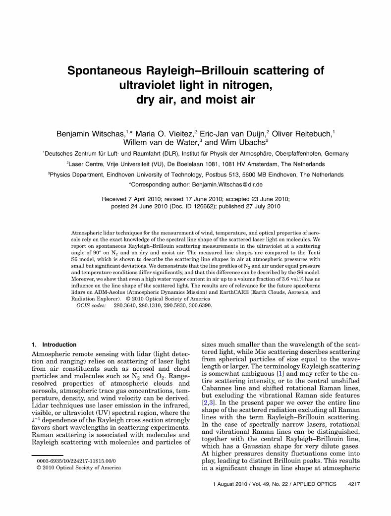
The influence of density fluctuations on the lineshape of the scattered light is largest when thewavenumber of soundmatches the size of the scatter-ing wave vector of light, k ¼ 2 ki sinðθ=2Þ, where ki isthe wave vector of the incident beam and θ is thescattering angle. Therefore, if cs is the velocity ofsound, the frequencies where the sound peaks occurin the scattered light frequency spectrum are shiftedfrom the central frequency by Δf ¼ �cs2 sinðθ=2Þ=λ,with λ the wavelength of the incident beam. Withcs ¼ ðγkBT=MÞ1=2, M as the mass of a molecule, γ ¼1:4 as the heat capacity ratio when no vibrationaldegrees of freedom are excited, and kB ¼ 1:38 ×10−23 J=K as the Boltzmann constant, the frequencyshift is about 1:3 GHz for the typical conditions of ourexperiment (λ ¼ 366:5 nm, θ ¼ 90°, and T ¼ 300 K).A few model spectra for different gas conditions areshown in Fig. 1.

For the backscattering of UV light in air at atmo-spheric pressures, the scattering wavelength be-comes of the order of the mean free path betweencollisions of the molecules. A key parameter is theratio y of the scattering wavelength 2π=k to the meanfree path between collisions [14],

y ¼ pkv0η

¼ nkBTkv0η

; ð1Þ

with n as the number density, T as the temperature,p as the pressure, v0 as the most probable thermalvelocity, v0 ¼ ð2kBT=MÞ1=2, and η as the shear viscos-ity. The definition of y is based on the dimensionalrelation between the mean free path between colli-sions and the shear viscosity η.

For y ≫ 1, the hydrodynamic regime, the meanfree path between collisions is much smaller thanthe scattering wavelength. In that case, the gas

can be treated as a continuum, and the spectrumof the scattered light can be calculated using theNavier–Stokes equations. The resulting spectrumcan be well approximated by the sum of three Lorent-zians displaced by Δf [35]. In the Knudsen regime,y ≪ 1, the mean free path between collisions is muchlarger than the scattering wavelength. Scattering issolely due to individual thermal molecules, and theline profile is described by the Rayleigh distributionaccording to

Iðk;ωÞ ¼ 2π1=2kv0

e−ðω=k v0Þ2: ð2Þ

In the kinetic regime 0:3≲ y≲ 3, which is therelevant regime for atmospheric scattering (y ≈0:1–0:4 for standard atmospheric conditions [36],λ ¼ 355 nm, θ ¼ 180°), neither the individual parti-cle approach nor the continuum approach applies,and one has to resort to solutions of the Boltzmannequation for the density fluctuations [37]. The Boltz-mann equation expresses the dynamical behavior ofthe position–velocity probability density f ðx; v; tÞ ofmolecules. Moments of f ðx; v; tÞ provide the transportequations of mass, momentum, and energy of conti-nuum physics, together with expressions of thetransport coefficients in terms of the collision crosssections. A linear system arises if the deviation ofthe probability density function from thermal equili-brium is expanded in eigenfunctions of the linearcollision operator. A line shape model results aftertruncation of this expansion to six or seven terms.It was shown in [14] that, from these two truncations,the six-moment model (the Tenti S6 model) providesthe superior fit of experimentally measured lineshapes. The line shapes for these different cases, cal-culated by means of the Tenti S6 model, are sketchedin Fig. 1.

While the truncation is one element of the model,the other one is the approximation to the linear colli-sion operator, which embodies elastic and inelasticcollisions between molecules. As detailed collisioncross sections are not available, the collision operatoris constructed such that the moments reproduce theknown values of the transport coefficients. This re-construction can be done in several ways. The theoryof Taxman [38] describes the internal degrees of free-dom of a molecule classically, and the semiclassicaltheory of Wang-Chang and Uhlenbeck [39] treatsthose degrees of freedom quantum-mechanicallybut does not deal with degenerate states. This pro-blem was cured in the model by Waldmann and Sni-der [40]. The Tenti S6 model uses the collision modelof Wang-Chang and Uhlenbeck, which needs thevalues of shear viscosity, heat conductivity, heatcapacity of internal degrees of freedom, and bulkviscosity of the gas under description. The valuesof these transport coefficients are well documented,except for the bulk viscosity ηb.

The bulk viscosity has its origin in the relaxation ofthe energy involving internal degrees of freedom ofmolecules to a change of the kinetic energy. In case

Fig. 1. Line shapes of SRB scattered light according to the TentiS6 model (wavelength λ ¼ 366:5 nm, scattering angle θ ¼ 90°) innitrogen for different scattering regimes. The black curve is repre-sentative for the Knudsen regime (y ¼ 0, for p≃ 0 hPa,T ¼ 293 K), the dashed black curve for the kinetic regime(y ¼ 0:56, for p ¼ 1000 hPa, T ¼ 293 K), and the gray curve forthe hydrodynamic regime (y ¼ 5:6, for p ¼ 10000 hPa,T ¼ 293 K). Curves are normalized to yield unity integrated inten-sity. The gas transport parameters of nitrogen that are used forsimulation can be found in Table 1.


of thermal equilibrium, the internal and the kinetictemperature are the same, but it may take many col-lisions to equilibrate the two. Therefore, the bulkviscosity depends on the structure of a moleculeand is essentially frequency-dependent [41,42].Wakeham [43] reviewed the status of the study oftransport properties of gases and pointed out thatthe shear viscosity as well as the thermal conductiv-ity can be measured with an accuracy of better than1% and that data are available for almost all di-atomic gases. In contrast to that, the bulk viscositydetermination for molecular gases is quite error-prone, which leads to a serious shortage in bulk visc-osity data [44]. Practically, there is only one singlemeasurement technique available for bulk viscosity[45], which utilizes sound absorption measurements.However, the errors of this indirect measurementtechnique are found to range up to 25% or larger [46].A more grave problem is that these measurementsare done at acoustic frequencies (up to 105 Hz), whilelight scattering involves frequencies that are four or-ders of magnitude larger. As the bulk viscosity isstrongly frequency dependent, its value at frequen-cies of the order of gigahertz must be considered lar-gely unknown. In order to establish a value for ηb wewill use spontaneous Rayleigh–Brillouin line shapemeasurements at a pressure of 3000 hPa in combina-tion with the S6 model. As no other measurementtechnique can reach the high frequencies of lightscattering, this is an unavoidable procedure.

The Tenti S6 line shape model is, as for almost allline shape models, restricted to gases consisting of asingle species. However, air is a mixture that we willtreat as an “effective” medium, consisting of mole-cules with an effective mass whose collisions areparametrized by effective transport coefficients.Therefore, we shall first present light scattering ex-periments on pure nitrogen and compare them to theTenti S6 model, and then compare experiments onair to the S6 model using the effective medium ap-proach. This procedure enables us to estimate theerror, which is made by describing the line shapeof scattered light in air using the S6 model withtransport coefficients of nitrogen, as it was done inthe past [5,19]. Furthermore, it gives us the possibi-lity to verify if the line shape prediction is improved ifthe appropriate transport coefficients (those for air)are used.

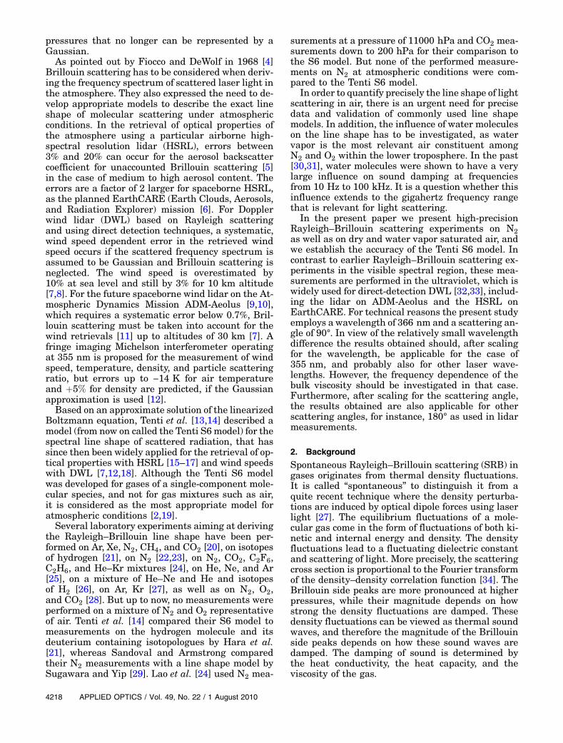
We investigate the role of the water vapor contentin air, which can reach up to 4 vol:%within the atmo-sphere (e.g., tropical conditions with water vaporsaturated air, p ¼ 1013 hPa, T ¼ 30 °C). Thus, watervapor might be the largest contributor to air after N2and O2. Water vapor is known to have a large andfrequency-dependent influence on the damping ofsound. According to sound absorption measurements[30], the bulk viscosity of water vapor saturated airat frequencies of the order of 10 kHz is one order ofmagnitude larger than that of dry air. These trendsare shown in Fig. 2, which shows the bulk viscosityfor both water vapor saturated and dry air depending

on sound frequency, based on an empirical formulapublished in [31]. The largest frequency consideredin this formula is the rotational relaxation frequencyof N2 and O2, after which the bulk viscosity drops tozero. While this might be adequate for the acousticalfrequencies for which this formula was designed, it isunrealistic at sound frequencies corresponding tooptical wavelengths. Figure 2 also suggests that theinfluence of water vapor is restricted to low frequen-cies, but it should be realized that the contribution ofthe relaxation process at much higher frequencies isnot known.

3. Experimental Details

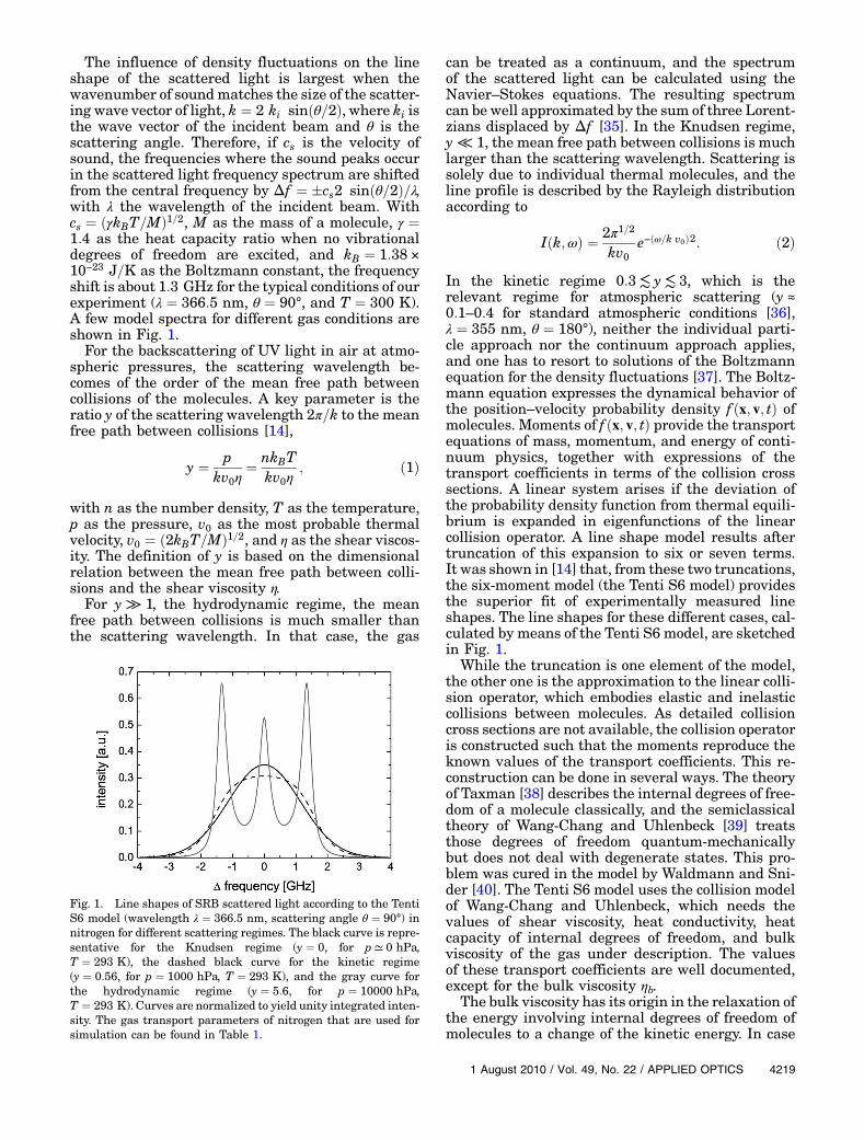
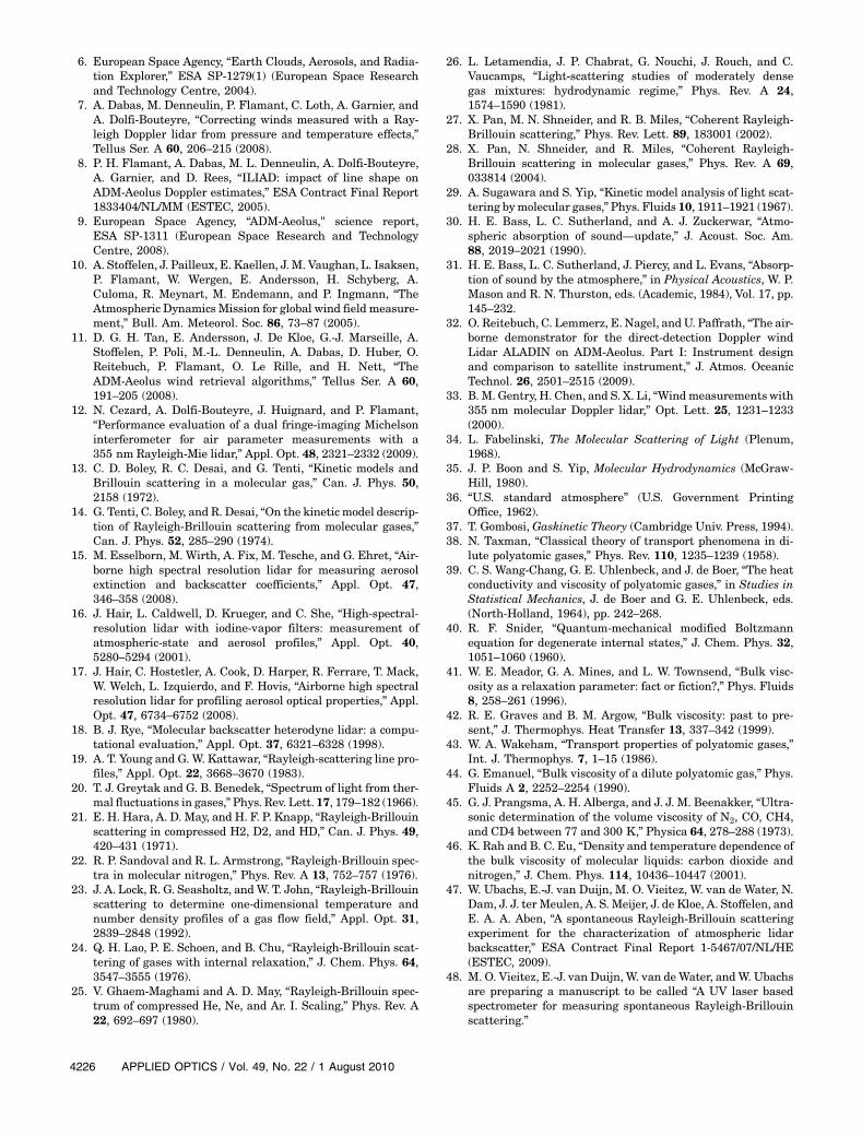
A block diagram of the experimental setup used tomeasure Rayleigh–Brillouin scattering (at Vrije Uni-versiteit, Amsterdam) is shown in Fig. 3. A more de-tailed description of the experimental setup andinstrument specifications can be found in [47,48].

The measured line shape of scattered radiation isthe result of the convolution of the real molecularprofile and the instrument function, which itself is

Fig. 2. Bulk viscosity ηb of dry (dashed line) and water-saturated(solid line) air as a function of frequency. The lines represent anempirical formula that is based on sound absorption measure-ments with sound frequencies up to 105 Hz [31].

Fig. 3. Schematic diagram of the experimental setup. The UVlaser beam (thick solid line), emitted from the laser source (LS),is reflected several times in the enhancement cavity (EC) to in-crease the scattering intensity. A reference beam (dashed line),split off of the main beam, is used for detector alignment. Thein the scattering cell (SC) scattered light (thin solid line) is de-tected at 90° using a pinhole, a Fabry–Perot interferometer(FPI), and a photomultiplier (PMT).


the result of the convolution of the laser bandwidthand the transmission bandwidth of the Fabry–Perotinterferometer. To avoid an influence of the laserbandwidth in the detected signal, a narrowband, con-tinuous wave, single longitudinal mode laser is used.The laser is a titanium sapphire (Ti:Sa) laser thatis pumped by a frequency doubled Nd:YVO4 laser(Millennia), delivering single-mode continuous waveradiation at 732 nm wavelength with an outputpower of 1:5 W. The laser bandwidth is 1 MHz at732 nm and the long-term frequency drift is mea-sured with a wavelength meter to be smaller than10 MHz per hour at 732 nm. After frequency dou-bling in a nonlinear optical crystal, laser light witha wavelength of 366:5 nm, 2 MHz linewidth, andpower of 400 mW is obtained. The UV beam is splitto obtain a main beam that is directed into an en-hancement cavity and a weaker reference beam thatis employed to align the system. The SRB-scatteredlight is collected at an angle of 90° from an auxiliaryfocus inside the enhancement cavity, in which a scat-tering cell (SC) is mounted. The cell is sealed withBrewster windows for not impeding the amplifica-tion of the UV circulating power, which reaches a fac-tor of 10, and hence a power level of 4 Wat 366:5 nm.The scattering angle is calculated to be 90°� 0:9° bymeans of the reference laser beam and geometricalrelations using sets of diaphragms and pinholes pre-sent in the optical setup. In a few cases, slightly bet-ter fits of the model spectra to the measurementscould be obtained by selecting the scattering angleθ from this interval. The scattered light is filteredby a diaphragm that covers an opening angle of 2°,collected by a set of lenses, further filtered by an ex-tra pinhole (d ¼ 50 μm), and is then directed into ascanning Fabry–Perot interferometer (FPI), whichis used to resolve the frequency spectrum of the scat-tered light. The FPI is built as a hemisphericalversion of a confocal etalon, which means that it iscomposed of one spherical and one plane mirror[49]. To scan the FPI plate distance, the sphericalmirror is mounted on a piezo-electrical translator,controlled by a computer. Despite the lower lightgathering in comparison to a plane parallel FPI (com-posed of two plane mirrors), the hemispherical con-figuration was chosen because of its insensitivity tosmall changes in tilt and orientation that can occurduring scanning. The transmission function of theFPI, which is the instrument function of the experi-ment, is described by using the Airy function accord-ing to [49,50]

Tðf Þ ¼ I0

�1þ

�2ΓFSR

πΔf FWHM

�sin2

� πΓFSR

f

��−1; ð3Þ

where I0 is the transmission maximum, ΓFSR is thefree spectral range, and Δf FWHM is the full width athalf-maximumof the transmission curve.ΓFSR, whichis the spectral distance between two intensity maxi-ma, was measured as 7:44 GHz. This is large enoughto resolve the spectrumofmolecular scattered light in

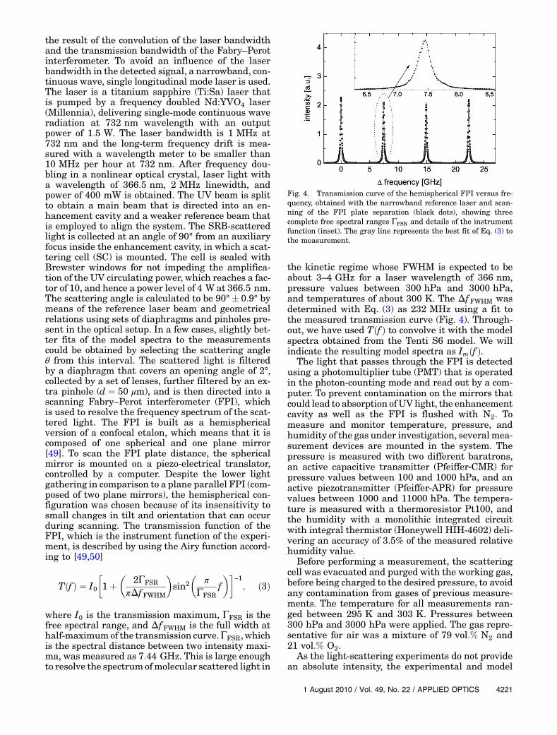
the kinetic regime whose FWHM is expected to beabout 3–4 GHz for a laser wavelength of 366 nm,pressure values between 300 hPa and 3000 hPa,and temperatures of about 300 K. The Δf FWHM wasdetermined with Eq. (3) as 232 MHz using a fit tothe measured transmission curve (Fig. 4). Through-out, we have used Tðf Þ to convolve it with the modelspectra obtained from the Tenti S6 model. We willindicate the resulting model spectra as Imðf Þ.

The light that passes through the FPI is detectedusing a photomultiplier tube (PMT) that is operatedin the photon-counting mode and read out by a com-puter. To prevent contamination on the mirrors thatcould lead to absorption ofUV light, the enhancementcavity as well as the FPI is flushed with N2. Tomeasure and monitor temperature, pressure, andhumidity of the gas under investigation, several mea-surement devices are mounted in the system. Thepressure is measured with two different baratrons,an active capacitive transmitter (Pfeiffer-CMR) forpressure values between 100 and 1000 hPa, and anactive piezotransmitter (Pfeiffer-APR) for pressurevalues between 1000 and 11000 hPa. The tempera-ture is measured with a thermoresistor Pt100, andthe humidity with a monolithic integrated circuitwith integral thermistor (Honeywell HIH-4602) deli-vering an accuracy of 3.5% of the measured relativehumidity value.

Before performing a measurement, the scatteringcell was evacuated and purged with the working gas,before being charged to the desired pressure, to avoidany contamination from gases of previous measure-ments. The temperature for all measurements ran-ged between 295 K and 303 K. Pressures between300 hPa and 3000 hPa were applied. The gas repre-sentative for air was a mixture of 79 vol:% N2 and21 vol:% O2.

As the light-scattering experiments do not providean absolute intensity, the experimental and model

Fig. 4. Transmission curve of the hemispherical FPI versus fre-quency, obtained with the narrowband reference laser and scan-ning of the FPI plate separation (black dots), showing threecomplete free spectral ranges ΓFSR and details of the instrumentfunction (inset). The gray line represents the best fit of Eq. (3) tothe measurement.


spectra were normalized such thatR f b−f b

Iðf Þdf ¼ 1.Ideally, the bounds f b of the integration should besuch that intensity is zero at f ¼ f b; however, the freespectral range of the etalon is not much larger thanthe width of the measured spectra. Therefore, wetake f b ¼ f fsr=2 in the normalization.

Another problem is the signal background Ie0 inthe experiment, which must be subtracted fromthe raw measured spectrum Ierðf Þ before normaliza-tion of Ieðf Þ ¼ Ierðf Þ − Ie0. It turns out that Ie0 is notjust the dark current of the photomultiplier, but alsocontains a small contribution, I0e0 of broadband fluor-escence of the cell windows. Therefore, it was decidedto correct the model spectra Imðf Þ for this poorlyknown background contribution, by setting Imðf Þ ¼aIeðf Þ − I0e0 , and determining I0e0 and the proportion-ality constant a in a least squares procedure for thewings of the spectra. If the measured spectra wouldhave the correct background, a ¼ 1 and I0e0 ¼ 0. Thewings of the spectra were defined as frequencies suchthat Imðf Þ ≤ maxðImÞ=4. The corrected model spec-trum I0mðf Þ ¼ Imðf Þ þ I0e0 was then normalized againsuch that

R f b−f b

I0mðf Þdf ¼ 1. This procedure gives asmall but perceptible change of the background in-tensity; it increased the wing intensity Imðf fsr=2Þby approximately 25%. In conclusion, in comparingexperimental to model line shapes, both the offsetand the scale of the vertical axis of the experimentalresult are chosen to match that of the modelspectrum.

Assuming Poisson statistics of the collected photoncounts, it is possible to arrive at an estimate of thestatistical error σðf iÞ at each (discrete) frequency ofthe data. This enables us to express the differencebetween measured spectrum Ieðf Þ and modeled spec-trum Imðf Þ as a χ2 value,

χ2 ¼ ð1=NÞXNi¼1

Ieðf iÞ − Imðf iÞÞ2σ2ðf iÞ

; ð4Þ

and thus to quantify the significance of the differencebetween experiment and model. This is importantas the number of photons collected for each spec-trum varies and is typically smallest at the lowestpressures.

4. Experimental Results

A. Comparison of N2 and Air

A key point of this study is the question of how wellthe Tenti S6 model reproduces the line shape innitrogen and air, and whether the line shape of spon-taneous Rayleigh–Brillouin scattering in air can beexplained by using the transport coefficients of nitro-gen. Therefore, SRB measurements on N2 and air atpressure ranges from 300 to 3000 hPa and tempera-tures of 295.5 to 301 K were performed and com-pared to the Tenti S6 model.

As explained in Section 2, the value of the bulkviscosity should be considered poorly known at soundfrequencies of the order of 1 GHz, at which values

they are relevant for SRB scattering. In order to ob-tain a value for ηb, we therefore adopted the followingprocedure: at a pressure of p ¼ 3000 hPa, the influ-ence of Brillouin scattering on the spectrum is large,and therefore its sensitivity to the used value of ηb inthe S6 model is large. Therefore, these pressures de-fine a value of ηb at frequencies of about 1:3 GHz,where the S6 model fits the experiment best. Thisprocedure, including the estimate of the uncertaintyin the obtained ηb, will be described in a follow-uppaper [51]. Summarizing, for N2 we thus found ηb ¼ð2:2� 0:5Þ × 10−5 kg m−1 s−1, which is about a factorof 1.7 larger than the literature value of 1:29 ×10−5 kg m−1 s−1 [28,44], while for air, ηb ¼ ð1:5�0:3Þ × 10−5 kg m−1 s−1, which is a factor of about1.4 larger than the literature value of 1:1 ×10−5 kg m−1 s−1 [52]. All transport coefficientsused for the model calculations are summarized inTable 1 [52,53].

The measured spectra for N2 and air at pressuresof 2000 and 3000 hPa, the comparison to the Tenti S6model, and the residuals with respect to the peak in-tensity are shown in Fig. 5. The corresponding spec-tra at 3000 hPa were used to establish the value ofthe bulk viscosity, which was then used for all othermodel calculations. Significant differences betweenthe S6 model and the measured spectra exist. For N2we find χ2 ¼ 5 at 2000 hPa and χ2 ¼ 7 at 3000 hPa,while for air χ2 ¼ 9 at 2000 hPa and χ2 ¼ 4 at3000 hPa. On a relative scale these differences aresmall; for N2 at 3000 hPa the error is 3%, and forair at 2000 hPa it is 2.6%.

To clarify further the difference of SRB spectra ob-tained in pure N2 and air and to show the capabilityof predicting this difference using the S6 model, wecalculate the residual plots between both spectra (N2and air) obtained at almost the same measurementconditions (Table 2). The difference between the N2and air spectra is quantified in two ways. First thestatistical significance of this difference is illustratedby plotting the normalized frequency-dependentdifference,

Δðf iÞ ¼IN2

ðf iÞ − Iairðf iÞðσN2

ðf iÞ2 þ σairðf iÞ2Þ1=2; ð5Þ

where σN2and σair are the statistical errors of the

measured N2 and air spectra assuming Poisson

Table 1. Gas Transport Coefficients Used for S6 Model Calculations

N2 Air

Mass number [g mol−1] 28.013 28.85Shear viscosity η [kg m−1 s−1] (1:79 × 10−5)a (1:846 × 10−5)b

Bulk viscosity ηb [kg m−1 s−1] (2:2 × 10−5)c (1:5 × 10−5)c

Thermal conductivity κ [W m−1 K−1] (25:5 × 10−3)a (26:24 × 10−3)b

Heat capacity ratio γ 1.4 1.4aValid at reference temperature 300 K. Taken from [53].bValid at reference temperature 300 K. Taken from [52].cValid at reference temperature 297 K, and frequency 1:3 GHz.

Taken from measurements (see Subsection 4.A).


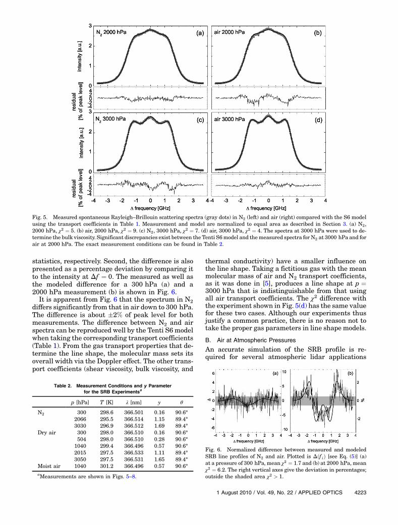
statistics, respectively. Second, the difference is alsopresented as a percentage deviation by comparing itto the intensity at Δf ¼ 0. The measured as well asthe modeled difference for a 300 hPa (a) and a2000 hPa measurement (b) is shown in Fig. 6.

It is apparent from Fig. 6 that the spectrum in N2differs significantly from that in air down to 300 hPa.The difference is about �2% of peak level for bothmeasurements. The difference between N2 and airspectra can be reproduced well by the Tenti S6 modelwhen taking the corresponding transport coefficients(Table 1). From the gas transport properties that de-termine the line shape, the molecular mass sets itsoverall width via the Doppler effect. The other trans-port coefficients (shear viscosity, bulk viscosity, and

thermal conductivity) have a smaller influence onthe line shape. Taking a fictitious gas with the meanmolecular mass of air and N2 transport coefficients,as it was done in [5], produces a line shape at p ¼3000 hPa that is indistinguishable from that usingall air transport coefficients. The χ2 difference withthe experiment shown in Fig. 5(d) has the same valuefor these two cases. Although our experiments thusjustify a common practice, there is no reason not totake the proper gas parameters in line shape models.

B. Air at Atmospheric Pressures

An accurate simulation of the SRB profile is re-quired for several atmospheric lidar applications

Fig. 5. Measured spontaneous Rayleigh–Brillouin scattering spectra (gray dots) in N2 (left) and air (right) compared with the S6 modelusing the transport coefficients in Table 1. Measurement and model are normalized to equal area as described in Section 3. (a) N2,2000 hPa, χ2 ¼ 5. (b) air, 2000 hPa, χ2 ¼ 9. (c) N2, 3000 hPa, χ2 ¼ 7. (d) air, 3000 hPa, χ2 ¼ 4. The spectra at 3000 hPa were used to de-termine the bulk viscosity. Significant discrepancies exist between the Tenti S6model and themeasured spectra for N2 at 3000 hPa and forair at 2000 hPa. The exact measurement conditions can be found in Table 2.

Fig. 6. Normalized difference between measured and modeledSRB line profiles of N2 and air. Plotted is Δðf iÞ [see Eq. (5)] (a)at a pressure of 300 hPa, mean χ2 ¼ 1:7 and (b) at 2000 hPa, meanχ2 ¼ 6:2. The right vertical axes give the deviation in percentages;outside the shaded area χ2 > 1.

Table 2. Measurement Conditions and y Parameterfor the SRB Experimentsa

p [hPa] T [K] λ [nm] y θ

N2 300 298.6 366.501 0.16 90:6°2066 295.5 366.514 1.15 89:4°3030 296.9 366.512 1.69 89:4°

Dry air 300 298.0 366.510 0.16 90:6°504 298.0 366.510 0.28 90:6°

1040 299.4 366.496 0.57 90:6°2015 297.5 366.533 1.11 89:4°3050 297.5 366.531 1.65 89:4°

Moist air 1040 301.2 366.496 0.57 90:6°aMeasurements are shown in Figs. 5–8.


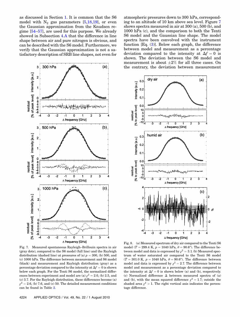
as discussed in Section 1. It is common that the S6model with N2 gas parameters [5,18,19], or eventhe Gaussian approximation from the Knudsen re-gime [54–57], are used for this purpose. We alreadyshowed in Subsection 4.A that the difference in lineshape between air and pure nitrogen is obvious, andcan be described with the S6 model. Furthermore, weverify that the Gaussian approximation is not a sa-tisfactory description of SRB line shapes, not even for

atmospheric pressures down to 300 hPa, correspond-ing to an altitude of 10 km above sea level. Figure 7shows spectra measured in air at 300 (a), 500 (b), and1000 hPa (c), and the comparison to both the TentiS6 model and the Gaussian line shape. The modelspectra have been convolved with the instrumentfunction [Eq. (3)]. Below each graph, the differencebetween model and measurement as a percentagedeviation compared to the intensity at Δf ¼ 0 isshown. The deviation between the S6 model andmeasurement is about �2% for all three cases. Onthe contrary, the deviation between measurement

Fig. 7. Measured spontaneous Rayleigh–Brillouin spectra in air(gray dots), compared to the S6 model (full line) and the Rayleighdistribution (dashed line) at pressures of (a) p ¼ 300, (b) 500, and(c) 1000 hPa. The difference between measurement and S6 model(black) and measurement and Rayleigh distribution (gray) as apercentage deviation compared to the intensity atΔf ¼ 0 is shownbelow each graph. For the Tenti S6 model, the normalized differ-ences between experiment and model are (a) χ2 ¼ 2:0, (b) 2.5, and(c) 3.7. For the Rayleigh distribution, these differences become (a)χ2 ¼ 2:6, (b) 7.6, and (c) 50. The detailed measurement conditionscan be found in Table 2.

Fig. 8. (a) Measured spectrum of dry air compared to the Tenti S6model (T ¼ 299:4 K, p ¼ 1040 hPa, θ ¼ 90:6°). The difference be-tween model and data is expressed by χ2 ¼ 3:1. (b) Measured spec-trum of water saturated air compared to the Tenti S6 model(T ¼ 301:0 K, p ¼ 1040 hPa, θ ¼ 90:6°). The difference betweenmodel and data is expressed by χ2 ¼ 2:7. The difference betweenmodel and measurement as a percentage deviation compared tothe intensity at Δf ¼ 0 is shown below (a) and (b), respectively.(c) Normalized difference Δ between measured spectra of (a)and (b), with the mean squared difference χ2 ¼ 1:7; outside theshaded area χ2 > 1. The right vertical axis indicates the percen-tage difference.


and Gaussian approximation is about �9% for anambient pressure of 1000 hPa (≈ sea level), and stillabout �3% for an ambient pressure of 300 hPa(≈ 10 km above sea level). This clearly demonstratesthat the Gaussian approximation is inadequateat pressures of 500 and 1000 hPa, while it is stillsignificantly worse than the Tenti S6 model atp ¼ 300 hPa.

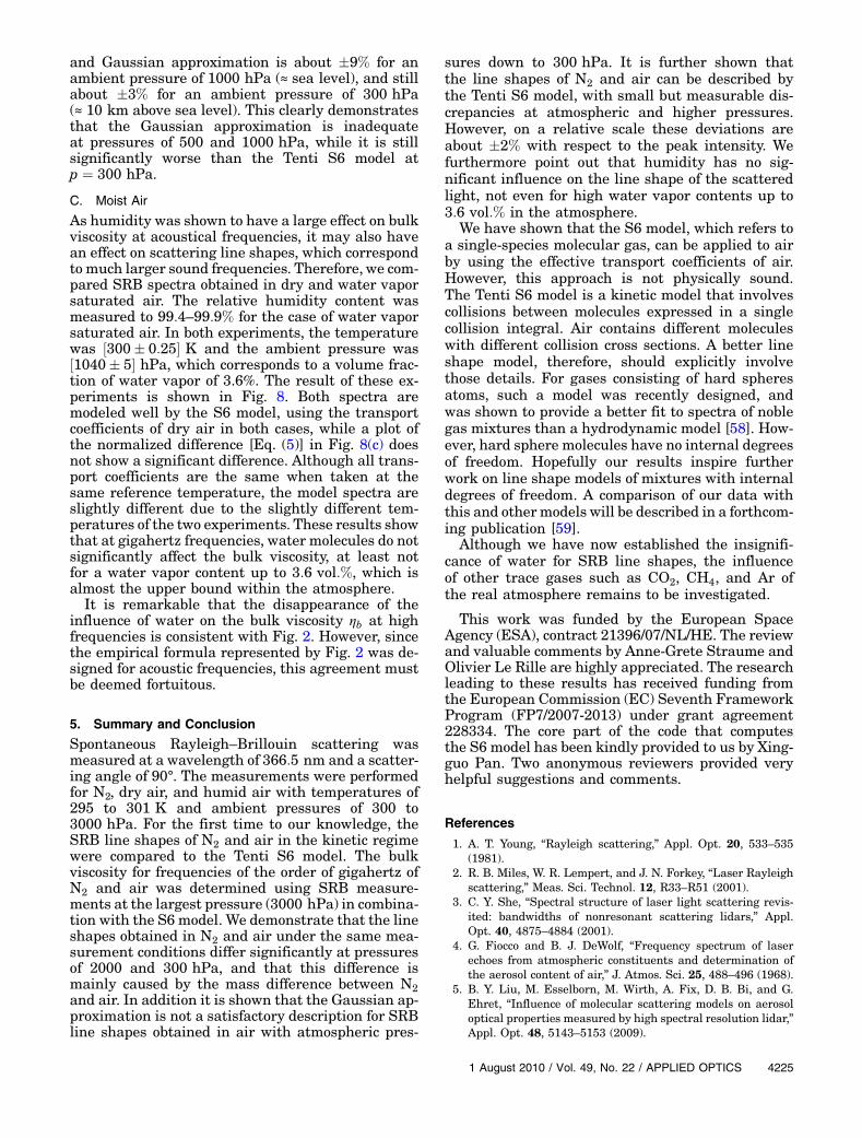
C. Moist Air

As humidity was shown to have a large effect on bulkviscosity at acoustical frequencies, it may also havean effect on scattering line shapes, which correspondto much larger sound frequencies. Therefore, we com-pared SRB spectra obtained in dry and water vaporsaturated air. The relative humidity content wasmeasured to 99:4–99:9% for the case of water vaporsaturated air. In both experiments, the temperaturewas ½300� 0:25� K and the ambient pressure was½1040� 5� hPa, which corresponds to a volume frac-tion of water vapor of 3.6%. The result of these ex-periments is shown in Fig. 8. Both spectra aremodeled well by the S6 model, using the transportcoefficients of dry air in both cases, while a plot ofthe normalized difference [Eq. (5)] in Fig. 8(c) doesnot show a significant difference. Although all trans-port coefficients are the same when taken at thesame reference temperature, the model spectra areslightly different due to the slightly different tem-peratures of the two experiments. These results showthat at gigahertz frequencies, water molecules do notsignificantly affect the bulk viscosity, at least notfor a water vapor content up to 3:6 vol:%, which isalmost the upper bound within the atmosphere.

It is remarkable that the disappearance of theinfluence of water on the bulk viscosity ηb at highfrequencies is consistent with Fig. 2. However, sincethe empirical formula represented by Fig. 2 was de-signed for acoustic frequencies, this agreement mustbe deemed fortuitous.

5. Summary and Conclusion

Spontaneous Rayleigh–Brillouin scattering wasmeasured at a wavelength of 366:5 nm and a scatter-ing angle of 90°. The measurements were performedfor N2, dry air, and humid air with temperatures of295 to 301 K and ambient pressures of 300 to3000 hPa. For the first time to our knowledge, theSRB line shapes of N2 and air in the kinetic regimewere compared to the Tenti S6 model. The bulkviscosity for frequencies of the order of gigahertz ofN2 and air was determined using SRB measure-ments at the largest pressure (3000 hPa) in combina-tion with the S6 model. We demonstrate that the lineshapes obtained in N2 and air under the same mea-surement conditions differ significantly at pressuresof 2000 and 300 hPa, and that this difference ismainly caused by the mass difference between N2and air. In addition it is shown that the Gaussian ap-proximation is not a satisfactory description for SRBline shapes obtained in air with atmospheric pres-

sures down to 300 hPa. It is further shown thatthe line shapes of N2 and air can be described bythe Tenti S6 model, with small but measurable dis-crepancies at atmospheric and higher pressures.However, on a relative scale these deviations areabout �2% with respect to the peak intensity. Wefurthermore point out that humidity has no sig-nificant influence on the line shape of the scatteredlight, not even for high water vapor contents up to3:6 vol:% in the atmosphere.

We have shown that the S6 model, which refers toa single-species molecular gas, can be applied to airby using the effective transport coefficients of air.However, this approach is not physically sound.The Tenti S6 model is a kinetic model that involvescollisions between molecules expressed in a singlecollision integral. Air contains different moleculeswith different collision cross sections. A better lineshape model, therefore, should explicitly involvethose details. For gases consisting of hard spheresatoms, such a model was recently designed, andwas shown to provide a better fit to spectra of noblegas mixtures than a hydrodynamic model [58]. How-ever, hard sphere molecules have no internal degreesof freedom. Hopefully our results inspire furtherwork on line shape models of mixtures with internaldegrees of freedom. A comparison of our data withthis and othermodels will be described in a forthcom-ing publication [59].

Although we have now established the insignifi-cance of water for SRB line shapes, the influenceof other trace gases such as CO2, CH4, and Ar ofthe real atmosphere remains to be investigated.

This work was funded by the European SpaceAgency (ESA), contract 21396/07/NL/HE. The reviewand valuable comments by Anne-Grete Straume andOlivier Le Rille are highly appreciated. The researchleading to these results has received funding fromthe European Commission (EC) Seventh FrameworkProgram (FP7/2007-2013) under grant agreement228334. The core part of the code that computesthe S6 model has been kindly provided to us by Xing-guo Pan. Two anonymous reviewers provided veryhelpful suggestions and comments.

References

1. A. T. Young, “Rayleigh scattering,” Appl. Opt. 20, 533–535(1981).

2. R. B. Miles, W. R. Lempert, and J. N. Forkey, “Laser Rayleighscattering,” Meas. Sci. Technol. 12, R33–R51 (2001).

3. C. Y. She, “Spectral structure of laser light scattering revis-ited: bandwidths of nonresonant scattering lidars,” Appl.Opt. 40, 4875–4884 (2001).

4. G. Fiocco and B. J. DeWolf, “Frequency spectrum of laserechoes from atmospheric constituents and determination ofthe aerosol content of air,” J. Atmos. Sci. 25, 488–496 (1968).

5. B. Y. Liu, M. Esselborn, M. Wirth, A. Fix, D. B. Bi, and G.Ehret, “Influence of molecular scattering models on aerosoloptical properties measured by high spectral resolution lidar,”Appl. Opt. 48, 5143–5153 (2009).


6. European Space Agency, “Earth Clouds, Aerosols, and Radia-tion Explorer,” ESA SP-1279(1) (European Space Researchand Technology Centre, 2004).

7. A. Dabas, M. Denneulin, P. Flamant, C. Loth, A. Garnier, andA. Dolfi-Bouteyre, “Correcting winds measured with a Ray-leigh Doppler lidar from pressure and temperature effects,”Tellus Ser. A 60, 206–215 (2008).

8. P. H. Flamant, A. Dabas, M. L. Denneulin, A. Dolfi-Bouteyre,A. Garnier, and D. Rees, “ILIAD: impact of line shape onADM-Aeolus Doppler estimates,” ESA Contract Final Report1833404/NL/MM (ESTEC, 2005).

9. European Space Agency, “ADM-Aeolus," science report,ESA SP-1311 (European Space Research and TechnologyCentre, 2008).

10. A. Stoffelen, J. Pailleux, E. Kaellen, J. M. Vaughan, L. Isaksen,P. Flamant, W. Wergen, E. Andersson, H. Schyberg, A.Culoma, R. Meynart, M. Endemann, and P. Ingmann, “TheAtmospheric Dynamics Mission for global wind field measure-ment,” Bull. Am. Meteorol. Soc. 86, 73–87 (2005).

11. D. G. H. Tan, E. Andersson, J. De Kloe, G.-J. Marseille, A.Stoffelen, P. Poli, M.-L. Denneulin, A. Dabas, D. Huber, O.Reitebuch, P. Flamant, O. Le Rille, and H. Nett, “TheADM-Aeolus wind retrieval algorithms,” Tellus Ser. A 60,191–205 (2008).

12. N. Cezard, A. Dolfi-Bouteyre, J. Huignard, and P. Flamant,“Performance evaluation of a dual fringe-imaging Michelsoninterferometer for air parameter measurements with a355 nm Rayleigh-Mie lidar,” Appl. Opt. 48, 2321–2332 (2009).

13. C. D. Boley, R. C. Desai, and G. Tenti, “Kinetic models andBrillouin scattering in a molecular gas,” Can. J. Phys. 50,2158 (1972).

14. G. Tenti, C. Boley, and R. Desai, “On the kinetic model descrip-tion of Rayleigh-Brillouin scattering from molecular gases,”Can. J. Phys. 52, 285–290 (1974).

15. M. Esselborn, M. Wirth, A. Fix, M. Tesche, and G. Ehret, “Air-borne high spectral resolution lidar for measuring aerosolextinction and backscatter coefficients,” Appl. Opt. 47,346–358 (2008).

16. J. Hair, L. Caldwell, D. Krueger, and C. She, “High-spectral-resolution lidar with iodine-vapor filters: measurement ofatmospheric-state and aerosol profiles,” Appl. Opt. 40,5280–5294 (2001).

17. J. Hair, C. Hostetler, A. Cook, D. Harper, R. Ferrare, T. Mack,W. Welch, L. Izquierdo, and F. Hovis, “Airborne high spectralresolution lidar for profiling aerosol optical properties,” Appl.Opt. 47, 6734–6752 (2008).

18. B. J. Rye, “Molecular backscatter heterodyne lidar: a compu-tational evaluation,” Appl. Opt. 37, 6321–6328 (1998).

19. A. T. Young and G. W. Kattawar, “Rayleigh-scattering line pro-files,” Appl. Opt. 22, 3668–3670 (1983).

20. T. J. Greytak and G. B. Benedek, “Spectrum of light from ther-mal fluctuations in gases,” Phys. Rev. Lett. 17, 179–182 (1966).

21. E. H. Hara, A. D. May, and H. F. P. Knapp, “Rayleigh-Brillouinscattering in compressed H2, D2, and HD,” Can. J. Phys. 49,420–431 (1971).

22. R. P. Sandoval and R. L. Armstrong, “Rayleigh-Brillouin spec-tra in molecular nitrogen,” Phys. Rev. A 13, 752–757 (1976).

23. J. A. Lock, R. G. Seasholtz, andW. T. John, “Rayleigh-Brillouinscattering to determine one-dimensional temperature andnumber density profiles of a gas flow field,” Appl. Opt. 31,2839–2848 (1992).

24. Q. H. Lao, P. E. Schoen, and B. Chu, “Rayleigh-Brillouin scat-tering of gases with internal relaxation,” J. Chem. Phys. 64,3547–3555 (1976).

25. V. Ghaem-Maghami and A. D. May, “Rayleigh-Brillouin spec-trum of compressed He, Ne, and Ar. I. Scaling,” Phys. Rev. A22, 692–697 (1980).

26. L. Letamendia, J. P. Chabrat, G. Nouchi, J. Rouch, and C.Vaucamps, “Light-scattering studies of moderately densegas mixtures: hydrodynamic regime,” Phys. Rev. A 24,1574–1590 (1981).

27. X. Pan, M. N. Shneider, and R. B. Miles, “Coherent Rayleigh-Brillouin scattering,” Phys. Rev. Lett. 89, 183001 (2002).

28. X. Pan, N. Shneider, and R. Miles, “Coherent Rayleigh-Brillouin scattering in molecular gases,” Phys. Rev. A 69,033814 (2004).

29. A. Sugawara and S. Yip, “Kinetic model analysis of light scat-tering bymolecular gases,” Phys. Fluids 10, 1911–1921 (1967).

30. H. E. Bass, L. C. Sutherland, and A. J. Zuckerwar, “Atmo-spheric absorption of sound—update,” J. Acoust. Soc. Am.88, 2019–2021 (1990).

31. H. E. Bass, L. C. Sutherland, J. Piercy, and L. Evans, “Absorp-tion of sound by the atmosphere,” in Physical Acoustics, W. P.Mason and R. N. Thurston, eds. (Academic, 1984), Vol. 17, pp.145–232.

32. O. Reitebuch, C. Lemmerz, E. Nagel, andU. Paffrath, “The air-borne demonstrator for the direct-detection Doppler windLidar ALADIN on ADM-Aeolus. Part I: Instrument designand comparison to satellite instrument,” J. Atmos. OceanicTechnol. 26, 2501–2515 (2009).

33. B. M. Gentry, H. Chen, and S. X. Li, “Windmeasurements with355 nm molecular Doppler lidar,” Opt. Lett. 25, 1231–1233(2000).

34. L. Fabelinski, The Molecular Scattering of Light (Plenum,1968).

35. J. P. Boon and S. Yip, Molecular Hydrodynamics (McGraw-Hill, 1980).

36. “U.S. standard atmosphere” (U.S. Government PrintingOffice, 1962).

37. T. Gombosi, Gaskinetic Theory (Cambridge Univ. Press, 1994).38. N. Taxman, “Classical theory of transport phenomena in di-

lute polyatomic gases,” Phys. Rev. 110, 1235–1239 (1958).39. C. S. Wang-Chang, G. E. Uhlenbeck, and J. de Boer, “The heat

conductivity and viscosity of polyatomic gases,” in Studies inStatistical Mechanics, J. de Boer and G. E. Uhlenbeck, eds.(North-Holland, 1964), pp. 242–268.

40. R. F. Snider, “Quantum-mechanical modified Boltzmannequation for degenerate internal states,” J. Chem. Phys. 32,1051–1060 (1960).

41. W. E. Meador, G. A. Mines, and L. W. Townsend, “Bulk visc-osity as a relaxation parameter: fact or fiction?,” Phys. Fluids8, 258–261 (1996).

42. R. E. Graves and B. M. Argow, “Bulk viscosity: past to pre-sent,” J. Thermophys. Heat Transfer 13, 337–342 (1999).

43. W. A. Wakeham, “Transport properties of polyatomic gases,”Int. J. Thermophys. 7, 1–15 (1986).

44. G. Emanuel, “Bulk viscosity of a dilute polyatomic gas,” Phys.Fluids A 2, 2252–2254 (1990).

45. G. J. Prangsma, A. H. Alberga, and J. J. M. Beenakker, “Ultra-sonic determination of the volume viscosity of N2, CO, CH4,and CD4 between 77 and 300 K,” Physica 64, 278–288 (1973).

46. K. Rah and B. C. Eu, “Density and temperature dependence ofthe bulk viscosity of molecular liquids: carbon dioxide andnitrogen,” J. Chem. Phys. 114, 10436–10447 (2001).

47. W. Ubachs, E.-J. van Duijn, M. O. Vieitez, W. van de Water, N.Dam, J. J. ter Meulen, A. S. Meijer, J. de Kloe, A. Stoffelen, andE. A. A. Aben, “A spontaneous Rayleigh-Brillouin scatteringexperiment for the characterization of atmospheric lidarbackscatter,” ESA Contract Final Report 1-5467/07/NL/HE(ESTEC, 2009).

48. M. O. Vieitez, E.-J. van Duijn, W. van deWater, andW. Ubachsare preparing a manuscript to be called “A UV laser basedspectrometer for measuring spontaneous Rayleigh-Brillouinscattering.”


49. G. Hernandez, Fabry-Perot Interferometers (Cambridge Univ.Press, 1988).

50. J. M. Vaughan, The Fabry-Perot Interferometer (AdamHilger, 1989).

51. W. van de Water, A. S. Meijer, A. S. de Wijn, M. Peters, and N.J. Dam, “Coherent Rayleigh-Brillouin scattering measure-ments of bulk viscosity of polar and nonpolar gases, and ki-netic theory,” J. Chem. Phys. (to be published).

52. T. D. Rossing, ed., Springer Handbook of Acoustics (Spring-er, 2007).

53. D. R. Lide, ed., CRCHandbook of Chemistry and Physics, 82thed. (CRC, 2002).

54. U. Paffrath, C. Lemmerz, O. Reitebuch, B. Witschas, I.Nikolaus, and V. Freudenthaler, “The airborne demonstratorfor the direct-detection Doppler wind Lidar ALADIN onADM-Aeolus. Part II: Simulations and Rayleigh receiverradiometric performance,” J. Atmos. Oceanic Technol. 26,2516–2530 (2009).

55. A. Ansmann, U. Wandinger, O. Le Rille, D. Lajas, and A.Straume, “Particle backscatter and extinction profilingwith the spaceborne high-spectral-resolution Doppler lidarALADIN: methodology and simulations,” Appl. Opt. 46,6606–6622 (2007).

56. M. McGill, W. Skinner, and T. Irgang, “Validation of wind pro-files measured with incoherent Doppler lidar,” Appl. Opt. 36,1928–1932 (1997).

57. D. Hua, M. Uchida, and T. Kobayashi, “UltravioletRayleigh-Mie lidar for daytime-temperature profiling of thetroposphere,” Appl. Opt. 44, 1315–1322 (2005).

58. J. R. Bonatto andW. Marquez, “Kinetic model analysis of lightscattering in binary mixtures of monoatomic ideal gases,”J. Stat. Mech. 9, 09014 (2005).

59. W. van de Water, M. O. Vieitez, E.-J. van Duijn, W. Ubachs, A.Meijer,A.S. deWijn,N. J.Dam,andB.Witschas, “Coherentandspontaneous Rayleigh-Brillouin scattering in atomic and mo-lecular gases, and gasmixtures,”Phys. Rev. A (to be published).


spontaneous rayleigh–brillouin scattering of ultraviolet light in nitrogen, dry air, and moist air

Documents