sponsored search marketing: dynamic pricing and advertising for an

Vol. 00, No. 0, Xxxxx 0000, pp. 000–000

issn 0000-0000 |eissn 0000-0000 |00 |0000 |0001

INFORMSdoi 10.1287/xxxx.0000.0000

c⃝ 0000 INFORMS

Sponsored Search Marketing: Dynamic Pricing andAdvertising for an Online Retailer

Shengqi Ye, Goker Aydin, Shanshan HuKelley School of Business, Indiana University, Bloomington, IN 47405

[email protected], [email protected], [email protected]

Consider a retailer using sponsored search marketing together with dynamic pricing. The retailer’s bid on

a search keyword affects the retailer’s rank among the search results. The higher the rank, the higher the

customer traffic and the customers’ willingness-to-pay will be. Thus, the question arises: When a retailer

bids higher to attract more customers, should the accompanying price also decrease (to strengthen the bid’s

effect on demand) or increase (to take advantage of higher willingness-to-pay)? We find that the answer

depends on how fast the retailer increases its bid. In particular, as the end of the season approaches, the

optimal bid exhibits smooth increases followed by big jumps. The optimal price increases only when the

optimal bid increases sharply, including the instances where the bid jumps up. Such big jumps arise, for

example, when the customer traffic is an S-shaped function of the retailer’s bid.

Key words : sponsored search marketing; dynamic pricing

1. Introduction

When using sponsored search marketing, the advertiser pays a search engine to display the adver-

tiser’s link in the search results page. Sponsored search is becoming an increasingly influential

advertising tool for many different sellers and service providers, especially for online retailers.

According to an industry survey conducted by PricewaterhouseCoopers, sponsored search spend-

ing in the United States hit $7.3 billion in the first half of 2011, up 27% compared to the same

half of 2010. The largest contributors have been retailers, who account for 23% of total sponsored

search spending (PwC and IAB 2011). Many of these retailers also use dynamic pricing, especially

online. When an online retailer uses dynamic pricing and sponsored search simultaneously, the

retailer has two levers to shape the demand. The first lever is the price. The second lever is the bid,

which indicates how much the retailer is willing to pay the search engine every time the retailer’s

link is clicked. The bid affects the rank of the retailer’s link in the search results page. The rank,

in turn, influences the customer traffic to the website and the customers’ willingness-to-pay (as

suggested by Ghose and Yang 2009, which we discuss later). The leverage enabled by the bid,

namely the ability to shape the customer traffic and willingness to pay, is not well studied in the

1

Ye, Aydin, and Hu: Sponsored Search Marketing2 00(0), pp. 000–000, c⃝ 0000 INFORMS

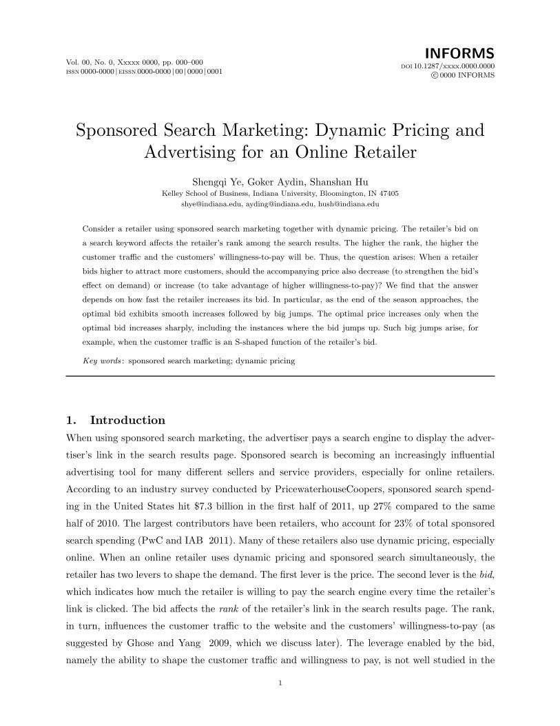
Figure 1 The Anecdotal Evidence: Online Bakery

08−23 08−27 08−31 09−04 09−08 09−12 (Moon Festival)

1

5

10

NA

Ra

nkin

g

Ranking

36

37

38

39

40

Price

1

58

60

62

Price

2

08−23 08−27 08−31 09−04 09−08 09−12 (Moon Festival)62

63

64

65

66

67

Time

Price

3

08−2708−27

Prices

09−0809−0808−29

08−29

Note: We recorded the rank and price at 10:00am and 7:00pm, for each day from 08/23/2011 to

09/12/2011. In the first graph, ranking “NA” means that the retailer’s link did not appear among the

sponsored links.

extant dynamic pricing literature. In this paper we study an online retailer’s dual use of sponsored

search and dynamic pricing. In so doing, we study a novel dynamic pricing problem in which the

retailer influences the customer traffic and willingness-to-pay by deciding how much to bid on a

keyword.

There is anecdotal evidence that online retailers are adjusting the two levers – the price and

the bid – simultaneously and dynamically. Consider the online branch of a Chinese bakery based

in Los Angeles.1 A signature product of this bakery is the mooncake, a dessert served during the

Chinese Moon Festival. The mooncake sales has strong seasonality, because consumers start buying

mooncakes about a month before the festival and rarely buy any after the festival is over. In 2011

the Moon Festival was on September 12. In the days leading to the Moon Festival, we tracked the

retailer’s rank among Google’s sponsored links (for keyword “mooncake”), as well as the posted

prices of three different mooncake packages on its website. Figure 1 shows the tracking results.

The figure suggests that the retailer used sponsored search and also adjusted the prices of the

three products dynamically. First, observe from the figure that the retailer’s ranking displayed

1 The bakery is called Kee Wah, and their online branch is http://keewah.us.

Ye, Aydin, and Hu: Sponsored Search Marketing00(0), pp. 000–000, c⃝ 0000 INFORMS 3

an “on-and-off” pattern, that is, its link either appeared at the top of the sponsored links, or

disappeared from the sponsored list entirely. While we do not observe the retailer’s bids on the

keyword “mooncake,” it is quite likely that the retailer was managing its bid so that its link, if

it appeared, would be among the top search results. Second, the retailer did not simply mark

down its prices as the Moon Festival was getting near. In fact, for the three products we tracked,

most discounts were offered in the middle of the selling season, indicating that the retailer utilized

dynamic pricing. Third, there were instances (marked by the three highlighted blocks) when changes

in rank were accompanied by price adjustments (for example, on September 8, the retailer’s link

reappeared at the top of search results page and the retailer increased the prices of products 1 and

3 on the same day). One suspects that the retailer might be coordinating its bid and price, rather

than managing them separately.

Two features of the online bakery’s business make it sensible to engage in both sponsored search

and dynamic pricing. This bakery is not a household name like Amazon. This makes it unlikely

that customers, especially first-time buyers, will land directly onto the bakery’s website. Spon-

sored search is thus the bakery’s primary method to attract internet customer traffic. In addition,

mooncake is a highly perishable product and the demand ceases after the Moon Festival. Hence,

dynamic pricing is a natural choice to profitably match demand with supply. Much like this online

bakery, there exist many online retailers who sell perishable products and rely on sponsored search

to attract the bulk of their customers. These retailers would benefit from the dual use of sponsored

search and dynamic pricing.

When using sponsored search and dynamic pricing simultaneously, a retailer must be mindful

of how the two strategies interact. Consider the potential profit earned by the retailer when a

customer clicks the retailer’s link and lands onto the retailer’s website. The retailer’s cost is simply

the bid. The retailer’s expected revenue from this customer is the price multiplied by the conversion

rate, i.e., the fraction of clicks that eventually convert to a sale. Hence, the bid and the price must

be determined together to generate a healthy profit margin. This decision is more complicated

than it appears at first blush, because the conversion rate itself depends on both the price and the

bid. Everything else being equal, the conversion rate decreases in the price and increases in the

bid. The latter effect, namely that higher bids lead to a higher conversion rate, is suggested by a

recent empirical study (Ghose and Yang 2009), which observes that as the bid increases and the

retailer’s link moves up, the conversion rate improves. Given these interactions between sponsored

search and dynamic pricing, an online retailer would do well to coordinate its bidding and pricing

decisions.

The research questions of this paper center on a retailer’s dual use of sponsored search and

dynamic pricing in the presence of inventory considerations. In particular, consider an online retailer


who is selling a limited inventory of a perishable product, for which the selling season has a

predetermined deadline. Suppose the inventory of the item is high relative to the time-to-go, i.e.,

the retailer finds itself “overstocked.” In such a case, the retailer needs to take action to increase

the demand. If the retailer is using dynamic pricing without sponsored search, the retailer’s course

of action is clear: decrease the price to sell more. Likewise, if the retailer is using sponsored search

without dynamic pricing, the retailer would choose to increase its bid, which increases customer

traffic and leads to higher willingness-to-pay. If, however, the retailer is using sponsored search

and dynamic pricing simultaneously, the retailer has a larger set of choices. Namely, we expect

that the retailer would take one of three actions: (1) The retailer could decrease the price and

increase the bid, both of which would increase the demand. (2) The retailer could decrease the

price, and if this causes a sufficient increase in demand, then the retailer could decrease its bid to

cut down its advertising cost. (3) The retailer could increase the bid, thereby increasing the traffic

and willingness-to-pay, which the retailer could exploit by increasing the price. Notice that the first

of these three actions uses the bid and the price to reinforce one another’s effect on demand. In

that sense, the first action uses the price and bid as complements. The latter two actions use only

one lever to increase the demand and they use the other lever in the opposite direction, with an

eye toward reducing cost or increasing revenue. In that sense, the latter two actions use the price

and bid as substitutes. These observations lead to our first research question:

(Q1) Given that both the bid and the price can shape the demand, should the retailer use them

as complements or substitutes?

When an overstocked retailer uses the price and the bid as complements, the lower price and

higher bid combine to increase the conversion rate. However, when the price and the bid are

substitutes, it is not clear how the conversion rate changes, because the bid and the price push the

conversion rate in opposite directions. This motivates our second research question:

(Q2) How does the conversion rate change as the retailer reacts to changes in inventory / time?

In addition, while the extant literature is rich in insights regarding dynamic pricing, not much is

known about the optimal dynamic bidding policy for an inventory-constrained retailer. As observed

in Figure 1, the retailer’s ranking exhibited an “on-and-off” pattern, which might have resulted

from the following “on-and-off” bidding policy: Either bid high enough to appear among the top

links or do not bid at all. Indeed, earlier literature suggested that similar bidding strategies may

arise due to competition (e.g., Zhang and Feng 2011). We investigate whether there may be other

explanations for the use of “on-and-off” bidding strategies. In particular, our third research question

is:

(Q3) Under what circumstances is it optimal to use “on-and-off” bidding?

Next, we position our work with respect to the extant literature. We include a summary of our

results in the conclusion.


2. Literature Review

Given our focus on an online retailer’s dual use of sponsored search and dynamic pricing, our

work is ultimately a study of dynamic pricing and advertising decisions for a product with limited

inventory. Thus, our work is related to the streams of literature on (i) dynamic pricing, (ii) dynamic

advertising, and (iii) interactions among pricing, advertising, and capacity.

Dynamic pricing: The dynamic pricing component of our work follows the literature on the

dynamic pricing of a seasonal product with fixed inventory. This stream of literature, pioneered by

Gallego and van Ryzin (1994) and Bitran and Mondschein (1997), studies how to adjust the price

based on the remaining inventory and time until the end of the selling season. While the models of

Gallego and van Ryzin (1994) and Bitran and Mondschein (1997) have been extended in several

directions, much of the earlier literature on dynamic pricing maintains the following assumption:

Neither the customer arrival rate nor the customers’ reservation price distribution depends on the

retailer’s decisions. Recently, two groups of papers have modified this assumption. The first group

includes papers that study dynamic pricing in the presence of strategic customer behavior (e.g.,

Su (2007), Aviv and Pazgal (2008), Elmaghraby et al. (2008), Levin et al. (2009), Liu and van

Ryzin (2011)). In such models, strategic customers anticipate the retailer’s actions and they decide

if and when to buy. In that sense, the effective willingness-to-pay and arrival rate are influenced

by the retailer’s decisions. The second group includes papers that study dynamic pricing in the

presence of reference price effects (e.g., Popescu and Wu (2006), Ahn et al. (2007), and Nasiry

and Popescu (2011)). In such models, the retailer’s earlier pricing decisions lead the customers to

form a reference price, which then influences the customers’ future willingness-to-pay.

Similarly, we model a situation where the retailer can influence the arrival rate and reservation

price of customers. In our model, such influence arises from the retailer’s ability to advertise

the product. In particular, the retailer in our model can improve both the arrival rate and the

reservation price by bidding higher to move up its sponsored link. MacDonald and Rasmussen

(2010) also consider a dynamic pricing problem where the retailer can influence the arrival rate

through advertising expenditure. A fundamental difference is that in our model the retailer is able

to influence the reservation price distribution while in their model the reservation price distribution

is exogenous. In addition, the retailer in their paper has full control over its advertising expenditure.

This is not the case for sponsored search: The retailer in our model pays a fee whenever a customer

clicks its link, hence its expenditure depends also on the stochastic customer arrivals. As we show,

these differences fundamentally change the trade-offs and deliver insights that are in sharp contrast

to those in MacDonald and Rasmussen (2010).

Dynamic advertising: There is a rich literature on dynamic advertising; see Feichtinger et al.

(1994) for an extensive review of earlier work. The dynamic advertising component of our work


focuses on a specific form of advertising, namely sponsored search. There is a growing body of

research on how a retailer can use sponsored search effectively. The economics literature on spon-

sored search treats the advertisers’ problem as bidding in an auction for “position” and focuses

on the bidding behavior that will arise in equilibrium (e.g., Aggarwal et al. (2006), Edelman et al.

(2007) and Varian (2007)). More recently, Edelman and Schwarz (2011) and Zhang and Feng

(2011) consider the equilibrium behavior of advertisers that are adjusting their bids over time in

dynamic auctions. Our focus is different as we do not aim to study the equilibrium behavior of

many advertisers. Instead, we adopt the perspective of an individual retailer who must make joint

pricing and bidding decisions in the presence of inventory considerations. To enable this focus, we

distill the effect of competition into a monotonic relationship between the bid and the arrival rate:

To attract more customers, the retailer needs to bid higher.

The marketing literature on sponsored search studies advertisers’ bidding decisions using models

that incorporate specific customer behavior issues. For example, Athey and Ellison (2009) and

Jerath et al. (2011) investigate advertisers’ optimal bidding strategy, by taking into account

consumers’ navigating and clicking behavior. Li et al. (2010) consider the advertiser’s bidding

strategy when the click rate is unknown in advance. Katona and Sarvary (2010) incorporate

customers’ choice between the list of organic search results and the list of sponsored links. Our

work differs from this literature in two ways. First, in this literature, the capacity constraint is often

neglected: A customer’s demand is guaranteed to be fulfilled once the customer is attracted to the

retailer’s website. In our model, this is not the case since the retailer has limited inventory with

no replenishment opportunity. Second, most papers in this stream assume an exogenous revenue

collected per click. In contrast, in our model, the price of the product, hence the revenue per click,

is endogenously determined by the retailer.

Because the conversion rate is an important performance metric in sponsored search marketing,

it appears as a factor in many of the above papers. For example, in the models of Athey and Ellison

(2009) and Katona and Sarvary (2010), the conversion rate is an input parameter. Our paper

adopts a different perspective on this important metric: In our model the conversion rate depends

on the retailer’s bid and price, which in turn are decisions that depend on the retailer’s inventory

and time until the end of the horizon.

Interactions among pricing, advertising, and capacity: Broadly speaking, our paper

explores the interactions among pricing, advertising, and capacity (given our focus on a retailer’s

pricing and bidding decisions in the presence of inventory considerations). Others have studied the

interaction between advertising and capacity, but in the absence of pricing decisions. For example,

Tan and Mookerjee (2005) consider a budget-constrained electronic retailer, who must trade-off


between sponsored search expenditure and website processing capacity. Chen et el. (2007) inves-

tigate the problem where an online retailer sells a perishable product and dynamically chooses

whether to promote the product by listing on a third-party channel. Swami and Khairnar (2006)

focus on a diffusion-type demand model for a product with limited availability, and they study the

retailer’s optimal advertising and, separately, optimal pricing.

Another group of papers study the interaction between pricing and advertising, but in the absence

of capacity considerations. For example, Albright and Winston (1979) investigate a firm’s optimal

advertising and pricing policy based on the firm’s market position, which is an abstract notion

that could capture, for example, the market share or the current sales level. In addition, Xu et al.

(2011) consider a setting where two advertisers compete over both link position and price, focusing

on the equilibrium behavior.

Other related research: Another related stream of research takes the perspective of a search

engine. The literature in this category generally considers two approaches to optimize the search

engine’s revenue. One of them is optimal auction design, for example, Ostrovsky and Schwarz

(2009), Liu et al. (2010) and Farboodi (2011). The main takeaway of these papers is that the

search engine should rank advertisers not only by their bids, but also by other factors such as

click-through rate. Another approach is more operations-oriented, considering the allocation of

limited advertising space to random advertising demand. The literature belonging to this category

includes Goel et al. (2010) and Asadolahi and Fridgeirsdottir (2011), the last of which provides

a review.

Besides theoretical papers, empirical work is also emerging. For example, Yao and Mela (2011)

empirically confirm that online retailers are practicing dynamic bidding, providing a validation for

our research motivation. Others investigate how click-through rate and conversion rate change with

respect to the rank of the link (Ghose and Yang 2009, Aggarwal et al. 2011), the interdependence

between organic and sponsored search results (Yang and Ghose 2010), the effect of an ad’s obtru-

siveness on purchase intent (Goldfarb and Tucker 2011), and so on. Some of these papers inform

our modeling choices, and they will be discussed later in more detail.

3. Model Description

Suppose the retailer has a fixed inventory of the product to sell within a predetermined selling

season. The retailer does not have the opportunity to replenish the inventory during the selling

season and the leftover inventory has zero value. Following the approach first adopted by Bitran

and Mondschein (1997), we divide the selling season into discrete periods, each of which is short

enough that at most one customer will click the retailer’s link during the period. Hereafter, the

click rate refers to the probability that a customer clicks the retailer’s link within one period. The


click rate is analogous to the arrival rate in the earlier literature on dynamic pricing (e.g., Bitran

and Mondschein 1997), with the very important exception that in our model the retailer can

influence the click rate by changing its bid on the search keyword.

At the beginning of each period t, the retailer chooses a keyword bid bt for its sponsored link

and submits it to the search engine. At the same time, the retailer determines a price pt for the

product, and posts it on the website. If a customer clicks the link during the period, the retailer

pays the search engine its bid bt.2 Subsequently, the customer makes a purchase if his reservation

price is above the posted price pt. From the retailer’s perspective, the reservation price of customers

who follow the link is a random variable with a known distribution. A key feature of our model is

that this reservation price distribution depends on the retailer’s bid on the search keyword. This

dependence arises because the bid influences the retailer’s rank in the search results page, thereby

affecting the customer mix attracted by the retailer.

Next, in Sections 3.1 and 3.2, we discuss our specific assumptions on how the retailer’s bid influ-

ences, respectively, the click rate and the reservation price distribution. In Section 3.3 we formulate

the retailer’s profit maximization problem as a dynamic program and we state preliminary results.

3.1. The Click Rate

The click rate of the retailer’s link depends on the link’s rank in the search results page. Most search

engines rank the links by taking into account both the retailer’s bid and the retailer’s relevance to

the search keyword. For instance, Google AdWords defines “relevance” to mean “the usefulness of

information (such as an ad, keyword, or landing page) to a user.”3 In particular, Google AdWords

uses the so-called “Quality Score” to measure a retailer’s relevance to a given search keyword. The

quality score is known to a potential advertiser, who can find that information in her AdWords

account statistics. For an online retailer who has a sufficiently long history with Google AdWords,

little can be done to change the quality score in the short term. Thus, the retailer’s main instrument

for moving up its rank is the bid. Through a higher bid, the retailer can achieve a higher rank,

which then results in a higher click rate. Instead of explicitly modeling the rank as an intermediary,

we use the abstraction formalized in the next assumption.

Assumption 1. In each period, the click rate λ(b) is a strictly positive, increasing, and twice

differentiable function in the retailer’s bid b.4

2 This assumption corresponds to the case where the search engine uses generalized first-price auction (i.e., the bidder’sper-click fee is equal to its bid). Other search engines use auctions similar to the generalized second-price auction(i.e., the bidder’s per-click fee is no more than its bid, and it depends on the bidder whose link is placed immediatelybelow). In the latter case, the per-click fee paid by the retailer is a stochastically increasing function of the retailer’sbid. Our model could accommodate this case because there is a one-to-one correspondence between the bid and theexpected per-click fee. Thus, we could extend our model by defining bt as the expected per-click fee.

3 See Google AdWords’ online help page, http://support.google.com/adwords/bin/answer.py?hl=en&answer=146307.

4 In this paper, we use the terms positive / negative, increasing / decreasing in the weak sense unless otherwise stated.


Of course, the retailer’s rank in the search results page depends not only on its own bid, but also

on competing bids from other advertisers. However, we do not model competition explicitly. Our

goal is not to capture the equilibrium bids of many advertisers who might be bidding on the same

search keyword. Instead, given our focus on a single retailer’s optimal bidding and pricing policy, it

is more meaningful to assume that a retailer, when making its bidding decision, relies on an estimate

of how the click rate depends on b. Hence, we adopt Assumption 1, which amounts to assuming

that the retailer knows the empirical relationship between its bid and the click rate. In fact, search

engines are assisting advertisers to estimate just such a relationship. For example, Google AdWords

provides a tool called “bid simulator,” which enables an advertiser to see retrospectively the results

it would have obtained if it had used a different bid. Similarly, Yahoo provides a forecast of how

the number of clicks and impressions will change if the advertiser adjusts its bid.

3.2. The Reservation Price Distribution

We assume that the customer decides whether or not to purchase only after clicking the retailer’s

link. In particular, upon following the link, the customer observes the posted price and purchases

the product if her reservation price is greater than the posted price. A key feature of our model

is that the retailer’s bid influences the reservation price distribution of customers who click the

retailer’s link. We adopt this assumption, because the bid influences the rank, which then influences

the mix of customers the retailer attracts. Specifically, letting Y (b) denote a customer’s reservation

price for a given bid b, we assume that Y (b) is given by:

Y (b) = µ(b)+σ(b)X, with µ(0) = 0 and σ(0) = 1. (1)

Here, X is the customer’s reservation price when the retailer bids zero. Let G(·) and g(·) denote thecumulative distribution function (cdf) and probability density function (pdf) of X. Equivalently,

if we denote the cdf of Y (b) as F (·|b), we may write

F (p|b) =G

(p−µ(b)

σ(b)

).

Intuitively, this formulation incorporates both the additive and multiplicative effects of the retailer’s

bid on the customer’s reservation price distribution.

In sponsored search marketing, the term “conversion rate” refers to the fraction of clicks that

lead to actual purchases. One can influence the conversion rate through the bid and the price.

Therefore, in the context of our model, which allows periodic bid and price adjustment, we define

the conversion rate in a given period as the probability that a customer purchases, given that she

clicked the retailer’s link in that period. Notice that, with this definition, the conversion rate is

essentially the probability that the reservation price Y (b) exceeds the posted price, i.e., F (p|b) :=1−F (p|b).

We impose the following assumption on the reservation price Y (b).


Assumption 2. Y (b) satisfies the following properties:

(a) The standard deviation of Y (b) is increasing in b. Equivalently, σ(b) is increasing.

(b) The coefficient of variation of Y (b) is decreasing in b. Equivalently, σ(b)/µ(b) is decreasing.

Given Assumption 2, as the bid increases, both the mean and the standard deviation of the

reservation price increases. However, Assumption 2(b) implies that the mean increases faster than

the standard deviation. In fact, Assumption 2(b) leads to an intuitive outcome, namely that the

reservation price Y (b) is stochastically increasing in the bid b. The following lemma states this

implication more formally.

Lemma 1. Assumption 2(b) implies that the reservation price, Y (b), is stochastically increasing

in the bid, b (in the sense of first-order stochastic dominance). In particular, when the support of

G(·) is the entire real line, Assumption 2(b) is equivalent to Y (b) stochastically increasing in b.

We next discuss the empirical and intuitive underpinnings of Assumption 2. Note that the

reservation price depends on the retailer’s bid only because the bid influences the rank of the

retailer’s link. To justify Assumption 2, let us first summarize two effects of the rank on the

customer mix attracted by the link – similar effects are also discussed in Ghose and Yang (2009)

(see Section 5.1.2 in their paper):

• The first effect is that a higher-ranked link attracts high-value customers, i.e., customers

with high reservation prices. There are many intuitive reasons for this effect. For example, some

customers may see a higher-ranked link as a sign of a more reliable retailer and, therefore, they

may be willing to pay more to purchase from that retailer. In addition, higher-ranked links attract

impatient customers, who tend to be less price sensitive. Furthermore, customers attracted by

higher-ranked links tend to visit fewer competing websites and, therefore, have fewer “outside

options.”

• The second effect runs counter to the first one. In addition to attracting high-value customers,

high-ranked links also attract window shoppers, who might click the top links without a serious

intent to purchase. Essentially, these are customers who have low reservation prices.

Assumption 2(a) follows from these two effects. High bids lead to high-ranked links, which attract

a diverse group of customers, including both high-value customers and window shoppers. Thus, a

higher bid leads to a customer mix whose reservation price exhibits a larger standard deviation.

Assumption 2(b), on the other hand, implies that the reservation price tends to increase in the

bid (as Lemma 1 indicates) and amounts to saying that the first effect outweighs the second effect.

In other words, the downward shift that window shoppers inflict on the reservation price of the

customer mix is more than canceled out by the upward shift caused by high-value customers. This

assumption is empirically supported by Ghose and Yang (2009), who find that “conversion rates


are highest at the top and decrease with rank as one goes down the search engine results page”

(page 11). In our model, the conversion rate is given by F (p|b), the probability that a customer’s

reservation price Y (b) exceeds the posted price. According to Lemma 1, as the retailer increases

its bid and its link moves up, this probability also increases, thus improving the conversion rate.

Therefore, Assumption 2(b) is consistent with Ghose and Yang’s empirical observation.

We should note that, in another recent empirical paper, Aggarwal et al. (2011) observe lower

conversion rates for higher ranks. That is, in their data set, the second effect (the influence of

window shoppers) dominates the first effect (the influence of high-value customers) and, hence, the

customers who click on higher-ranked links might actually have lower reservation prices on average.

Aggarwal et al. (2011) attribute the difference between their results and those of Ghose and Yang

(2009) primarily to the difference in the ranges of ranks studied by the two papers. Specifically,

Ghose and Yang (2009) evaluate conversion rates for ranks ranging from the top all the way down

to 131. In contrast, Aggarwal et al. (2011) focus on the top seven positions. Given that we wish to

model a retailer who is not restricted to remain among the top links, we believe that the empirical

observations of Ghose and Yang (2009) are more applicable in our setting.

Assumption 3 below is needed to ensure the quasi-concavity of the profit function.

Assumption 3. G(·) has an increasing failure rate (IFR).

In addition, we make the following technical assumption, which guarantees the smoothness of

the profit function.

Assumption 4. The following regularity conditions hold:

(a) The support of G(·) extends to positive infinity.

(b) If the support of G(·) has a lower bound, then its density is zero at this lower bound.

(c) G(·) has continuous first-order derivative within its support.

(d) µ(b) and σ(b) have continuous first-order derivatives.

The IFR property in Assumption 3 is satisfied by many standard probability distributions,

including the Normal distribution, Gamma and Weibull distributions with shape parameter strictly

greater than one. Assumption 4(a),(b) rule out certain IFR distributions such as Uniform, Beta,

and Exponential. For these distributions, it might be optimal to set the price at the lower or upper

bound of the support and, hence, there might be cases where it is optimal to sell to all or no

customers. Such cases add few new insights to our current results, but require messy algebra to

handle the end points of the support. Therefore, we choose to adopt Assumption 4(a)(b), which

lead to a simpler exposition.


Remark 1. For ease of exposition, we assumed that the functions λ(b), µ(b) and σ(b) are sta-

tionary. Following the approach in Zhao and Zheng (2000), we could extend our analysis to cover

the case where these functions are time-dependent. The key insights about the optimal bidding

and pricing policy will remain the same.

3.3. The Maximization Problem

Next we formulate the dynamic program for the retailer’s profit maximization problem. Our con-

vention is to count down the periods, with period T corresponding to the beginning of the horizon

and period 1 being the last period. Let Π(y, t) denote the retailer’s optimal expected profit when

starting period t with y units of inventory. The optimality equations are given by (we omit the

subscript t of bt and pt)

Π(y, t) = maxb≥0,p≥0

(1−λ(b))Π(y, t− 1)+λ(b)F (p|b) (Π(y, t− 1)− b)+λ(b)F (p|b) (p+Π(y− 1, t− 1)− b)

, for y > 0, t= 1, ..., T,

Π(0, t) = 0, for t= 1, ..., T,

Π(y,0) = 0, for y > 0.

The first term inside the maximization is the retailer’s expected profit-to-go in the event that no

customer clicks the link. The second term corresponds to the case where a customer clicks but does

not purchase the product. The third term is for the case where a customer clicks and purchases

the product. The retailer chooses its optimal posted price p and bid b at the beginning of period

t to maximize its profit-to-go. The terminal conditions indicate that no replenishment is possible

and that the salvage value of the item is zero.

After some algebraic manipulation, Π(y, t) can be rearranged as follows:

Π(y, t) =Π(y, t− 1)+ maxb≥0,p≥0

{λ(b)

[F (p|b) (p−∆(y, t))− b

]}, (2)

where we use notation ∆(y, t) :=Π(y, t−1)−Π(y−1, t−1). Here, ∆(y, t) can be interpreted as the

expected value of carrying one more unit of the product into period t− 1 when there are already

y − 1 units in inventory. In other words, ∆(y, t) denotes the marginal value of the y-th unit of

inventory in period t or, alternatively, the retailer’s opportunity cost of selling the y-th unit in

period t. Define

π(b, p,∆)= λ(b)[F (p|b)(p−∆)− b

]. (3)

Here, π(b, p,∆) can be interpreted as the expected marginal contribution from selling one unit of

the product in period t, given the retailer’s bid b, the price p, and the marginal value of inventory,

∆. Using (2) and (3), the retailer’s optimization problem becomes

Π(y, t) =Π(y, t− 1)+ maxb≥0,p≥0

π(b, p,∆(y, t)). (4)


The following results about ∆(y, t) are standard in dynamic pricing models and we therefore

present them as preliminary properties of the model.

Lemma 2. The marginal value of inventory, ∆(y, t), is decreasing in the inventory level y and

increasing in the time-to-go t.

We define the following notation, which will be convenient when referring to the retailer’s optimal

actions:

⟨b∗(∆), p∗(∆)⟩ : = argmaxb≥0,p≥0

π(b, p,∆),

⟨b∗(y, t), p∗(y, t)⟩ : = ⟨b∗(∆(y, t)), p∗(∆(y, t))⟩.

Following the interpretation of π(b, p,∆), ⟨b∗(∆), p∗(∆)⟩ is the optimal bid and posted price when

the retailer’s marginal value of inventory is some arbitrary number ∆. In particular, with y units in

inventory and t periods to go, the retailer’s marginal value of inventory is ∆(y, t), and the retailer’s

optimal bid and posted price are ⟨b∗(y, t), p∗(y, t)⟩.

Our analysis will focus on the optimal policy as a function of ∆, i.e., ⟨b∗(∆), p∗(∆)⟩, since it is

more convenient to establish the properties of the optimal policy in the context of the continuous

variable ∆. (We restrict ∆ so that ∆∈ [0,∆(1, T )], where ∆(1, T ) yields the largest possible value

for the marginal value of inventory, by Lemma 2.) We use the structure of this optimal policy to

explain the behavior of ⟨b∗(y, t), p∗(y, t)⟩, which is simply a discretization of ⟨b∗(∆), p∗(∆)⟩.

4. Structure of the Optimal Policy

In this section, we first establish several properties of the optimal bidding and pricing policy. These

properties allow us to identify two distinct structures of the optimal policy, both of which may arise

under our current set of assumptions. Later, in Section 5, we will identify how the assumptions

on the click rate and the reservation price are responsible for the differences between the two

structures.

4.1. The Optimal Bidding Policy

The next proposition describes the effects of time and inventory on the retailer’s optimal bid.

Proposition 1. The optimal bid as a function of the marginal value of inventory, i.e., b∗(∆),

decreases in ∆. Consequently, when the inventory increases or time-to-go decreases, the optimal

bid as a function of inventory and time-to-go, b∗(y, t), increases.

This monotonicity result is intuitive. With shorter time-to-go or higher inventory, the marginal

value of inventory decreases, that is, the opportunity cost of selling one unit of product in the

current period decreases. Thus, the retailer has more incentive to sell the unit within the current


period. As a result, the retailer increases the bid, thereby increasing the sponsored link’s click rate

and the reservation prices of the arriving customers.

Figure 2 depicts two examples of the optimal bidding policy. While both examples in Figure

2 exhibit the monotonicity properties established in Proposition 1, there is a marked difference

between them. In Example 1, for a fixed level of inventory, the optimal bid changes “smoothly”

in the time-to-go t. In Example 2, however, the optimal bid switches between two modes that can

be clearly distinguished: An “on” mode where the retailer sets a series of high bids, and an “off”

mode where the retailer simply bids 0.

Figure 2 Two Distinct Examples of Optimal Bidding Policy.

0510150.2

0.4

0.6

0.8

1

1.2

1.4

1.6

1.8

Optimal Bidding Strategy

Number of Remaining Periods

Op

tim

al B

id

0510150

0.5

1

1.5

Optimal Bidding Strategy


Op

tim

al B

id

I=2

I=4

I=6

Example 1 Example 2

Parameter setting: In both examples, σ(b) = 1+0.1b, and X is distributed with Gamma(6,0.5). In Example

1, we set µ(b) = 0.6b and λ(b) = 0.8−0.7e−b. In Example 2, we set µ(b) = 0.4b and λ(b) = (1+0.4e4−4b)/(1+

e4−4b).

The two examples in Figure 2 correspond to two distinct possibilities. The difference between

them is not cosmetic, but structural. In particular, the difference between these two examples is

rooted in the behavior of b∗(∆): In Example 1 the optimal bid b∗(∆) turns out to be continuous

in ∆, whereas in Example 2 it is discontinuous. In Example 2, as the time-to-go decreases, the

marginal value ∆ also decreases and passes through a discontinuity point of b∗(∆), thus leading to

the jumps observed. Note that the discontinuity arises even though all the input functions (e.g.,

the click rate, the reservation price distribution) are continuous and differentiable.

Hereafter, to distinguish between these two cases, we will refer to the smooth bidding policy

illustrated in Example 1 as single-mode bidding and we will refer to the on-and-off bidding policy


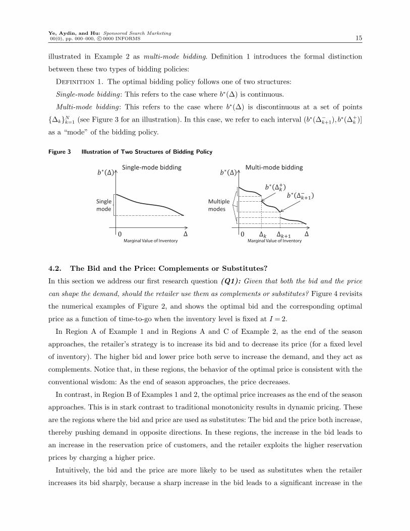
illustrated in Example 2 as multi-mode bidding. Definition 1 introduces the formal distinction

between these two types of bidding policies:

Definition 1. The optimal bidding policy follows one of two structures:

Single-mode bidding : This refers to the case where b∗(∆) is continuous.

Multi-mode bidding : This refers to the case where b∗(∆) is discontinuous at a set of points

{∆k}Nk=1 (see Figure 3 for an illustration). In this case, we refer to each interval (b∗(∆−k+1), b

∗(∆+k )]

as a “mode” of the bidding policy.

Figure 3 Illustration of Two Structures of Bidding Policy

Marginal Value of Inventory Marginal Value of Inventory

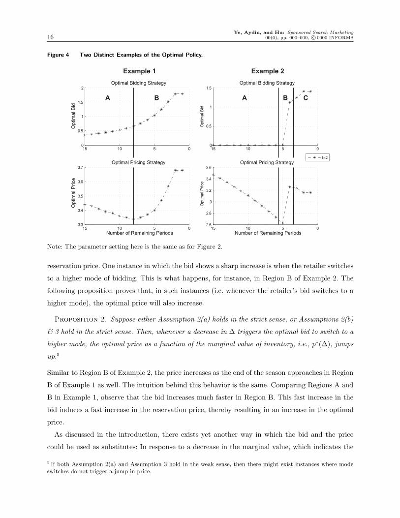
4.2. The Bid and the Price: Complements or Substitutes?

In this section we address our first research question (Q1): Given that both the bid and the price

can shape the demand, should the retailer use them as complements or substitutes? Figure 4 revisits

the numerical examples of Figure 2, and shows the optimal bid and the corresponding optimal

price as a function of time-to-go when the inventory level is fixed at I = 2.

In Region A of Example 1 and in Regions A and C of Example 2, as the end of the season

approaches, the retailer’s strategy is to increase its bid and to decrease its price (for a fixed level

of inventory). The higher bid and lower price both serve to increase the demand, and they act as

complements. Notice that, in these regions, the behavior of the optimal price is consistent with the

conventional wisdom: As the end of season approaches, the price decreases.

In contrast, in Region B of Examples 1 and 2, the optimal price increases as the end of the season

approaches. This is in stark contrast to traditional monotonicity results in dynamic pricing. These

are the regions where the bid and price are used as substitutes: The bid and the price both increase,

thereby pushing demand in opposite directions. In these regions, the increase in the bid leads to

an increase in the reservation price of customers, and the retailer exploits the higher reservation

prices by charging a higher price.

Intuitively, the bid and the price are more likely to be used as substitutes when the retailer

increases its bid sharply, because a sharp increase in the bid leads to a significant increase in the


Figure 4 Two Distinct Examples of the Optimal Policy.

0510150

0.5

1

1.5

2Optimal Bidding Strategy

Op

tim

al B

id

0510153.3

3.4

3.5

3.6

3.7Optimal Pricing Strategy


0510150

0.5

1

1.5Optimal Bidding Strategy

Op

tim

al B

id

0510152.6

2.8

3

3.2

3.4

3.6Optimal Pricing Strategy


Op

tim

al P

rice

Op

tim

al P

rice

Example 1 Example 2

A B A B C

I=2

Note: The parameter setting here is the same as for Figure 2.

reservation price. One instance in which the bid shows a sharp increase is when the retailer switches

to a higher mode of bidding. This is what happens, for instance, in Region B of Example 2. The

following proposition proves that, in such instances (i.e. whenever the retailer’s bid switches to a

higher mode), the optimal price will also increase.

Proposition 2. Suppose either Assumption 2(a) holds in the strict sense, or Assumptions 2(b)

& 3 hold in the strict sense. Then, whenever a decrease in ∆ triggers the optimal bid to switch to a

higher mode, the optimal price as a function of the marginal value of inventory, i.e., p∗(∆), jumps

up.5

Similar to Region B of Example 2, the price increases as the end of the season approaches in Region

B of Example 1 as well. The intuition behind this behavior is the same. Comparing Regions A and

B in Example 1, observe that the bid increases much faster in Region B. This fast increase in the

bid induces a fast increase in the reservation price, thereby resulting in an increase in the optimal

price.

As discussed in the introduction, there exists yet another way in which the bid and the price

could be used as substitutes: In response to a decrease in the marginal value, which indicates the

5 If both Assumption 2(a) and Assumption 3 hold in the weak sense, then there might exist instances where modeswitches do not trigger a jump in price.


retailer is now more overstocked, the retailer could reduce the price (to increase the demand) while

also reducing the bid (to cut down on the advertising costs). However, we now know that such

a pair of decisions would never arise in the optimal policy; Proposition 1 guarantees that when

the marginal value of inventory decreases, the optimal bid increases. Intuitively, reducing the bid

would reduce the reservation prices of the clicking customers and, thus, the retailer would have to

take unattractively large price cuts to stimulate more demand.

It is interesting that the online bakery’s bidding and pricing decisions on 8/27 and 9/8 are in

compliance with our optimal policy (see Figure 1). According to our optimal policy, when the bid

jumps (as it apparently did on 8/27 and 9/8), the price should jump in the same direction. This

is indeed what happened with the retailer’s price on those two days. Of course, we do not know

how the retailer’s inventory changed on those days, so we cannot say if their actions were indeed

optimal according to our model. We should also note that there are instances where the retailer’s

decisions violate our optimal policy. For example, on 8/29, it appears that the retailer turned on

its bid and reduced the prices of two products. Such a coupling of bidding and pricing decisions

would never be optimal under our model. This might be due to reasons outside of our model, for

example, the risk attitude of the decision maker or the actions of a competitor.

4.3. The Conversion Rate

Next we answer our second research question (Q2) How does the conversion rate change as the

retailer reacts to changes in inventory / time? Consider an increase in inventory (at a fixed time)

or a decrease in time-to-go (at a fixed inventory). Both changes put more pressure on the retailer

to move the inventory more quickly. When the bid and the price are complements, it is clear what

happens to the conversion rate: The bid increases and the price decreases, both of which improve the

conversion rate. However, when the bid and the price are substitutes, they will both increase, and

the net effect on the conversion rate is not clear. The higher bid lifts up the customers’ reservation

prices and, hence, increases the conversion rate, whereas the higher price decreases the conversion

rate. Nevertheless, we find that the effect of the bid always wins out over the effect of the price.

Hence, whenever the inventory increases or time-to-go decreases, the conversion rate increases.

Proposition 3. The conversion rate as a function of the marginal value of inventory,

F (p∗(∆)|b∗(∆)), decreases in ∆. Consequently, when the inventory increases or time-to-go

decreases, the conversion rate increases.

In essence, the proposition shows that, even when the retailer is using the bid and price as substi-

tutes, the change in price should not be so large as to override the effect of the bid on the conversion

rate.


5. When is Multi-Mode Bidding Policy Optimal?

In this section we turn to our third research question: (Q3) Under what circumstances it it optimal

to use “on-and-off” bidding? In Figure 2, we already observed a numerical example (Example 2),

in which “on-and-off” bidding policy was optimal. The on-and-off bidding policy is a special case of

the multi-mode bidding policy (see Definition 1), which arises when b∗(∆) is discontinuous. Next

we show that this discontinuity and, thus, the optimality of the multi-mode bidding policy, may

owe to the shape of the click rate function and properties of the reservation price distribution. In

what follows, to isolate the effects of the click rate and the reservation price, we first focus on the

case where only the click rate depends on the bid (in Section 5.1) followed by the case where only

the reservation price depends on the bid (in Section 5.2).

5.1. The Bid’s Effect on the Click Rate

Consider the case where the customer’s reservation price, Y (b), does not depend on the bid, b, while

the click rate, λ(b), does. As the next proposition states, the multi-mode bidding policy would

never arise if the click rate is a concave function of the bid.

Proposition 4. If the click rate, λ(b), is strictly concave in the bid, b, then the optimal bid,

b∗(∆), is continuous and a single-mode bidding policy is optimal.

This result sheds light on why the optimal bidding policy in Example 1 of Figure 2 was the single-

mode bidding policy, i.e., why the optimal bid did not exhibit any jumps. In that example, the

click rate was concave increasing in the bid.

When λ(b) is concave, the improvement in the click rate diminishes as the bid increases. This

assumption is realistic for high-end bids. After all, once the retailer’s link is the top-ranked link,

any further increase in the bid will not improve the click rate. However, one would expect that this

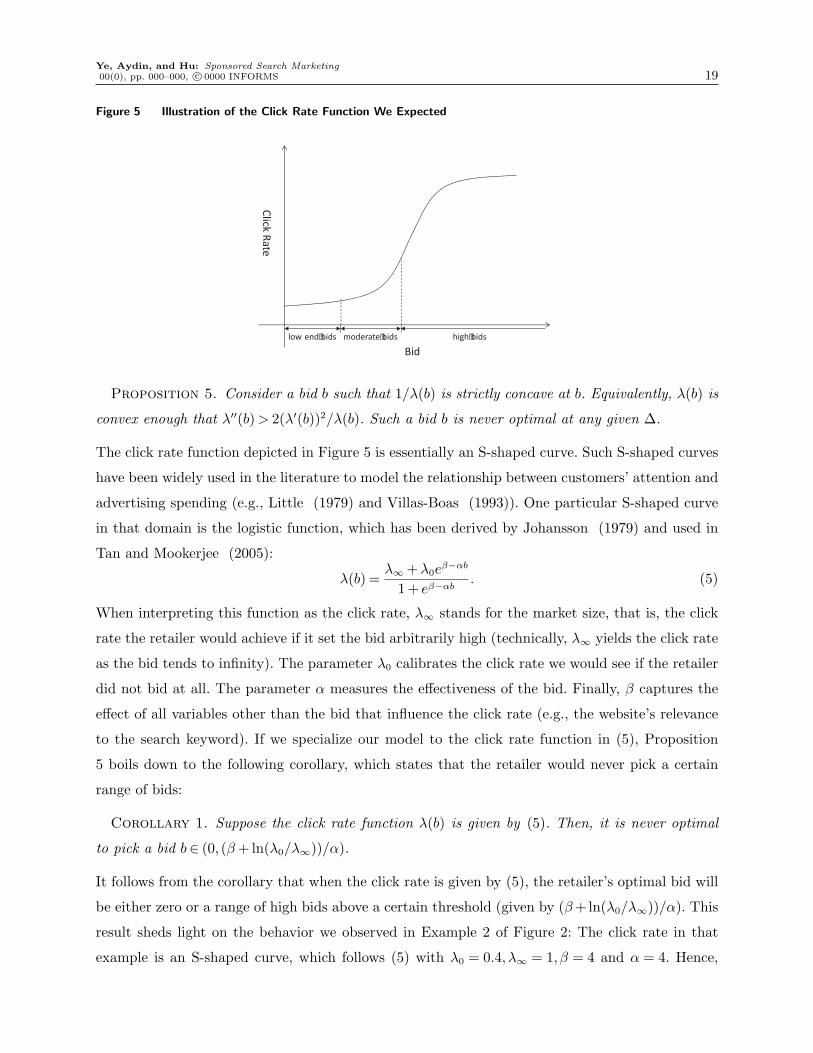
assumption does not hold at low to moderate bids. When the retailer sticks to low-end bids, the

link will appear towards the bottom of the page or, worse yet, the link will fall off the first page.

Few customers will scroll far down the page or go beyond the first page of search results. Hence, as

shown in Figure 5, we expect the click rate to be low and rather flat in the region of low-end bids.

As the bid keeps increasing, it will reach a moderate level that will catapult the link to the easily

visible range of search results, thus turning the click rate from flat to sharply increasing. Hence,

as depicted in Figure 5, we expect the click rate to have a convex region, corresponding to low to

moderate bids.

Intuitively, one would not pick a bid in the region where the click rate is turning from flat to

sharply increasing, because in that region the additional clicks brought by a marginally higher bid

is increasing very fast. In fact, the following proposition formalizes this result as it shows that a

bid b is never optimal if the click rate is sufficiently convex at that bid.


Figure 5 Illustration of the Click Rate Function We Expected

CClick

Rate

low end bids moderate bids high bids

Bid

Proposition 5. Consider a bid b such that 1/λ(b) is strictly concave at b. Equivalently, λ(b) is

convex enough that λ′′(b)> 2(λ′(b))2/λ(b). Such a bid b is never optimal at any given ∆.

The click rate function depicted in Figure 5 is essentially an S-shaped curve. Such S-shaped curves

have been widely used in the literature to model the relationship between customers’ attention and

advertising spending (e.g., Little (1979) and Villas-Boas (1993)). One particular S-shaped curve

in that domain is the logistic function, which has been derived by Johansson (1979) and used in

Tan and Mookerjee (2005):

λ(b) =λ∞ +λ0e

β−αb

1+ eβ−αb. (5)

When interpreting this function as the click rate, λ∞ stands for the market size, that is, the click

rate the retailer would achieve if it set the bid arbitrarily high (technically, λ∞ yields the click rate

as the bid tends to infinity). The parameter λ0 calibrates the click rate we would see if the retailer

did not bid at all. The parameter α measures the effectiveness of the bid. Finally, β captures the

effect of all variables other than the bid that influence the click rate (e.g., the website’s relevance

to the search keyword). If we specialize our model to the click rate function in (5), Proposition

5 boils down to the following corollary, which states that the retailer would never pick a certain

range of bids:

Corollary 1. Suppose the click rate function λ(b) is given by (5). Then, it is never optimal

to pick a bid b∈ (0, (β+ ln(λ0/λ∞))/α).

It follows from the corollary that when the click rate is given by (5), the retailer’s optimal bid will

be either zero or a range of high bids above a certain threshold (given by (β+ln(λ0/λ∞))/α). This

result sheds light on the behavior we observed in Example 2 of Figure 2: The click rate in that

example is an S-shaped curve, which follows (5) with λ0 = 0.4, λ∞ = 1, β = 4 and α = 4. Hence,


as the inventory or time-to-go changes, the retailer’s optimal bid is either zero or is found among

some high-end bids.

5.2. The Bid’s Effect on Customer’s Reservation Price

Next consider the case where the click rate, λ(b), is independent of the bid, b. We focus on the

the case where the randomness of the reservation price Y (b) is additive, i.e., we assume σ(b) to be

independent of b and we normalize it to 1 so that Y (b) = µ(b)+X. In this case, the bid influences

the reservation price only through its effect on µ(b), which shifts the mean. A result analogous to

Proposition 5 holds:

Proposition 6. A bid b > 0 is never optimal for any marginal value of inventory ∆ if µ′′(b)> 0

at b.

Proposition 6 suggests that the optimal bid never falls in the region where a marginally higher

bid shifts the reservation price with increasing speed. When the mean reservation price follows

the logistic form (analogous to the S-shaped curve in (5)), Proposition 6 leads to the following

corollary, which specifies the range of bids that will never be optimal.

Corollary 2. Suppose µ(b) is given by the logistic function, i.e., µ(b) = (µ∞ + µ0eβ−αb)/(1 +

eβ−αb). Then, it is never optimal to pick a bid b∈ (0, β/α).

Consequently, when the mean reservation price follows the logistic function, the retailer’s optimal

bid will be either zero or a range of high bids above a certain threshold.

6. A Heuristic: Static On-and-Off Bidding

We observed in Section 5 that on-and-off bidding might arise in the optimal solution as a special

case of the multi-mode bidding policy. When following the on-and-off bidding policy, the retailer

either bids zero (the “off” mode) or updates its bid within a high range as the inventory and time

change (the “on” mode). Observe from Example 2 of Figure 2 that the optimal bid lands within

a narrow band when the retailer’s bidding is on. Motivated by this observation, it is tempting to

consider a static version of the on-and-off bidding policy as a heuristic. In this heuristic, the retailer

would pick a bid for the “on” mode at the beginning of the selling season and, subsequently, the

retailer’s decision in each period would be whether to bid this predetermined amount or not bid

at all. In this section we analyze the performance of this heuristic, which we refer to as the static

on-and-off bidding policy.

To evaluate the performance of the heuristic policy, we conduct a numerical study. We consider

a retailer with 10 units in inventory and 15 periods to go. We let X follow a Gamma distribution

with shape parameter k and scale parameter θ. To generate problem instances, we let k take on


Table 1 Parameter Settings for Numerical Test

Parameter Set of Valuesk {1,3,5,7,9}α {1,2,3,4,5,6}β {1,2,3,4,5,6}λ0 {0.1,0.2,0.3,0.4,0.5,0.6}γµ {0.1,0.2,0.3,0.4}γσ {0.1,0.2,0.3,0.4}

Table 2 Statistics of the Optimality Gap

Statistics* Valuemean 0.28%standard deviation 0.25%maximum and minimum (0,1.37%]95% confidence interval [0,0.85%]

*When calculating the statistics, we ruled out all instances with zero optimality gap.

one of five different values ({1,3,5,7,9}) with θ chosen accordingly so that X has a mean of three.

We adopt the S-shaped click rate function in (5) with λ∞ normalized to be 1 and with each of λ0,

α and β taking one of six different values. In addition, we let

µ(b) = γµb and σ(b) = 1+ γσb,

where each of γµ and γσ can take one of four different values. Notice that when both µ(b) and

σ(b) are linear, Assumption 2 is satisfied. The parameter values used in our numerical study are

summarized in Table 1. All in all, we are testing 17,280 instances.

For each instance, we evaluate the optimality gap, i.e., the difference between the optimal

expected profit and the profit from the heuristic, expressed as a percentage of the optimal expected

profit. Table 2 provides summary statistics observed across 17,280 instances. (To avoid giving unfair

advantage to the heuristic, we removed instances where the optimality gap is zero; those are likely

to be the trivial instances where the optimal policy is not to make a bid throughout the season.) As

the summary statistics show, the static on-and-off bidding policy comes very close to the optimal

solution. In particular, in 95% of the instances, the optimality gap is less than 1%. On average,

the optimality gap is only 0.28%.

7. Conclusion

Sponsored search marketing has become a reliable marketing tool for online retailers to attract

customer traffic. In this paper, we investigate an online retailer’s dual use of sponsored search

marketing and dynamic pricing. Such decisions involve complicated trade-offs. On one hand, the

retailer faces the usual dynamic pricing trade-off: Too high a price may reduce the sales and lead

to leftover inventory, yet too low a price leaves money on the table. On the other hand, the retailer


needs to choose the right bid: It is unwise to bid so high as to unnecessarily sacrifice profit margin,

yet the bid should be high enough to generate sufficiently high traffic. However, the real challenge

is that there is an interaction between the pricing and bidding trade-offs: The retailer’s bid on the

keyword moves the rank of its sponsored link and, therefore, influences the customer’s reservation

price, which factors into the retailer’s pricing decision.

Based on a model that incorporates the above trade-offs and interactions, we identify the fol-

lowing structure for the optimal bidding policy. (Here we summarize how the optimal bid changes

with time; we obtained similar results for the effect of inventory.) For a fixed level of inventory,

as the retailer gets closer to the end of the season, the optimal bid increases. In particular, the

optimal bid exhibits smooth increases followed by big jumps. The monotonicity of the optimal

bid is intuitive: As the end of season approaches, the retailer is under increasing pressure to move

inventory, thus giving the retailer an incentive to advertise more aggressively. On the other hand,

the big jumps in the optimal bid occur when the click rate or the reservation price “takes off” once

the bid reaches a threshold. In such a case, the retailer will choose a bid beyond the take-off region.

This happens, for example, when the click rate is an S-shaped function of the bid.

As for the optimal pricing strategy: As the end of the season approaches and the bid increases, the

accompanying optimal price may increase or decrease. The case where the optimal price decreases

is intuitive – that is the case where the retailer is using both the bid and the price as complements

to move its inventory quickly as the end of the season is approaching. However, the case where

the optimal price increases is in contrast to the conventional wisdom of dynamic pricing. In those

instances, the retailer is now using the bid and price as substitutes. More specifically, those are

instances where a sharp increase in the bid (sometimes in the form of an upward jump) causes

a significant increase in the customers’ reservation prices, and the retailer increases the price to

exploit the higher willingness to pay. Furthermore, based on our model, it is never optimal for an

increase in bid to come together with a price decrease. In other words, if the retailer is following

the optimal strategy throughout, the retailer will never be so desperate as not to take advantage

of the increase in willingness-to-pay caused by a higher bid.

Our results also provide implementation notes for retailers using sponsored search marketing and

dynamic pricing together. When a retailer takes a break from bidding on a keyword, the retailer

might want to mark down its price simultaneously. Symmetrically, when a retailer starts bidding

again, it might want to increase its price. However, the increase in price should never be so high as

to cancel the improvement in conversion rate caused by the higher bid. In addition, our numerical

results indicate that, instead of adjusting the bid around the clock, the retailer can achieve similarly

good results using a static on-and-off bidding heuristic. When using this simple heuristic, depending

on time and inventory, the retailer switches between no bid and a predetermined static bid.


References

Albright, S. C., W. Winston. 1979. Markov Models of Advertising and Pricing Decisions. Operations Research

27 668–681.

Aggarwal, G., J. Feldman, S. Muthukrishnan. 2006. Bidding to the top: VCG and equilibria of position-based

auctions. Approximation and Online Algorithms. Lecture Notes in Computer Science. Springer, Berlin,

15–28.

Aggarwal, A., K. Hosanagar, M. D. Smith. 2011. Location, Location, Location: An Analysis of Profitability

of Position in Online Advertising Markets. Journal of Marketing Research. 48, 1057-1073.

Ahn, H.-S., M. Gumus, P. Kaminsky. 2007. Pricing and Manufacturing Decisions when Demand is a Function

of Prices in Multiple Periods. Operations Research 55 1039-1057.

Asadolahi, S. N., K. Fridgeirsdottir. 2011. Cost-Per-Click Pricing for Display Advertising. Working paper,

London Business School, Regent’s Park, London.

Athey, S., G. Ellision. 2009. Position Auctions with Consumer Search. Working paper, National Bureau of

Economic Research, Cambridge MA.

Aviv, Y., A. Pazgal. 2008. Optimal pricing of seasonal products in the presence of forward-looking consumers.

Manufacturing & Service Operations Management 10 339-359.

Bitran, G. R., R. Caldentey. 2003. Commissioned paper: An overview of pricing models for revenue manage-

ment. Manufacturing & Service Operations Management 5 203–229.

Bitran, G. R., S. V. Mondschein. 1997. Periodic pricing of seasonal products in retail. Management Science

43 64–79.

Chen, F. Y., J. Chen, Y. Xiao. 2007. Optimal Control of Selling Channels for an Online Retailer with

Cost-per-Click Payments and Seasonal Products. Production and Operations Management 16 292–305.

Edelman, B., M. Ostrovsky, M. Schwarz. 2007. Internet advertising and the generalized 2nd-price auction:

Selling billions of dollars worth of keywords. American Economic Review 97 242–259.

Edelman, B.G., M. Schwarz. 2011. Optimal Auction Design and Equilibrium Selection in Sponsored Search

Auctions. Working paper, Harvard Business School, Boston MA.

Elmaghraby, W., P. Keskinocak. 2003. Dynamic pricing in the presence of inventory considerations: Research

overview, current practices and future directions. Management Science 49 1287–1309.

Elmaghraby, W., A. Gulcu, P. Keskinocak. 2008. Designing optimal preannounced markdowns in the presence

of rational customers with multiunit demands. Manufacturing & Service Operations Management 10

126-148.

Farboodi, M. 2011. Optimal Revenue Maximizing Mechanism in Common-Value Position Auctions. Working

paper, University of Chicago, Chicago IL.

Feichtinger, G., R. F. Hartl, S. P. Sethi. 1994. Dynamic Optimal Control Models in Advertising: Recent

Developments. Management Science 40 195-226.


Gallego, G. & van Ryzin, G. 1994. Optimal dynamic pricing of inventories with stochastic demand over finite

horizions. Management Science 40 999–1020.

Ghose, A., S. Yang. 2009. An Empirical Analysis of Search Engine Advertising: Sponsored Search in Elec-

tronic Markets. Management Science 55 1605-1622.

Goel, A., M. Mahdian, H. Nazerzadeh, A. Saberi. 2010. Advertisement allocation for generalized second-

pricing schemes. Operations Research Letters 38 571-576.

Goldfarb, A., C. Tucker. 2011. Online Display Advertising: Targeting and Obtrusiveness. Marketing Science

30 389-404.

Helft, M. 2009. The Science of Managing Search Ads. The New York Times Dec. 21.

Jerath, K., L. Ma, Y-H. Park, K. Srinivasan. 2011. A “Position Paradox” in Sponsored Search Auctions.

Marketing Science Articles in Advance.

Johansson, J. K. 1979. Advertising and the S-Curve: A New Approach. Journal of Marketing Research 16

346-354.

Katona, Z., M. Sarvary. 2010. The Race for Sponsored Links: Bidding Patterns for Search Advertising.

Marketing Science 29 199-215.

Levin, Y., J. McGill, M. Nediak. 2009. Dynamic Pricing in the Presence of Strategic Consumers and

Oligopolistic Competition. Management Science 55 32-46.

Li, S-M., M. Mahdian, R. P. McAfee. 2010. Value of Learning in Sponsored Search Auctions. Lecture Notes

in Computer Science 6484 294-305.

Liu, D., J. Chen, A. B. Whinston. 2010. Ex Ante Information and the Design of Keyword Auctions. Infor-

mation Systems Research 21 133-153.

Liu, Q. and G. van Ryzin. 2011. Strategic Capacity Rationing when Customers Learn. Manufacturing &

Service Operations Management 13 89-107.

Little, J. D. C. 1979. Aggregate advertising models: The state of the art. Operations Research 27 629-667.

MacDonald, L., H. Rasmussen. 2010. Revenue Management with Dynamic Pricing and Advertising. Journal

of Revenue and Pricing Management 9 126–136.

Nasiry, J., I. Popescu. 2011. Dynamic Pricing with Loss-Averse Consumers and Peak-End Anchoring. Oper-

ations Research 59 1361–1368.

Osadchiy, N., G. Vulcano. 2010. Selling with Binding Reservations in the Presence of Strategic Consumers.

Management Science 56 2173–2190.

Ostrovsky, M., M. Schwarz. 2009. Reserve Prices in Internet Advertising Auctions: A Field Experiment.

Working paper, Stanford University Graduate School of Business.

PricewaterhouseCoopers(PwC), Interactive Advertising Bureau(IAB). September 2011. IAB Internet Adver-

tising Revenue Report (2011 First Six Months Results).


Popescu, I., Y. Wu. 2007. Dynamic Pricing Strategies with Reference Effects. Operations Research 55 413–

429.

Su, X. 2007. Intertemporal Pricing with Strategic Customer Behavior. Management Science 53 726-741.

Swami, S., P. J. Khairnar. 2006. Optimal normative policies for marketing of products with limited avail-

ability. Annals of Operations Research 143 107–121.

Tan, Y., V. S. Mookerjee. 2005. Allocating Spending Between Advertising and Information Technology in

Electronic Retailing. Management Science 51 1236-1249.

Varian, H. R. 2007. Position auctions. International Journal of Industrial Organization 25 1163–1178.

Villas-Boas, J. M. 1993. Predicting Advertising Pulsing Policies in an Oligopoly: A Model and Empirical

Test. Marketing Science 12 88-102.

Xu, L., J. Chen, A. Whinston. 2011. Price Competition and Endogenous Valuation in Search Advertising.

Journal of Marketing Research 48 566-586.

Yang, S., A. Ghose. 2010. Analyzing the Relationship Between Organic and Sponsored Search Advertising:

Positive, Negative, or Zero Interdependence? Marketing Science 29 602–623.

Yao, S., C. F. Mela. 2011. A Dynamic Model of Sponsored Search Advertising.Marketing Science 30 447-468.

Zhang, X., J. Feng. 2011. Cyclical Bid Adjustments in Search-Engine Advertising. Management Science 57

1703-1719.

Zhao, W., Y-S. Zheng. 2000. Optimal Dynamic Pricing for Perishable Assets with Nonhomogeneous Demand.

Management Science 46 375-388.

Appendix. Proofs

Additional Notation

We first define additional notation to be used throughout our proofs. In particular, in some instances, it will

be convenient to use the following change of variable to replace the price p:

ξ(b, p) :=p−µ(b)

σ(b).

Given this definition, F (p|b) can be written as G(ξ(b, p)). Hence, through the change of variable (x= ξ(b, p)),

the profit function in (3) can be rewritten as

π̃(b,x,∆) := λ(b)[G(x)(σ(b)x+µ(b)−∆)− b

], (A.1)

where x is treated as a decision variable. Define x∗(b,∆) as the optimal value of x given b and ∆, that is:

x∗(b,∆) := argmaxx

π̃(b, x,∆). (A.2)


In addition, define x∗(∆) as the optimal value of x when the retailer uses the optimal bid b∗(∆):

x∗(∆) = x∗(b∗(∆),∆).

Notice that the relationship between x∗(∆) and the optimal price p∗(∆) is given by:

p∗(∆) = µ(b∗(∆))+σ(b∗(∆))x∗(∆). (A.3)

Further, we define the induced profit function, π(b,∆), as the profit obtained by maximizing π̃(b,x,∆) over

x:

π(b,∆)=maxx

π̃(b,x,∆)= π̃(b, x∗(b,∆),∆).

Alternatively, the induced profit function π(b,∆) can also be obtained by maximizing π(b, p,∆) over p:

π(b,∆)=maxp

π(b, p,∆).

Supporting Lemmas

Next we develop two supporting lemmas about ξ(b, p) and x∗(b,∆) that will be used by later proofs.

Lemma A.1. ξ(b, p) is increasing in p and decreasing in b.

Proof of Lemma A.1: The monotonicity of ξ(b, p) in p is clear from its definition. It is decreasing in b since

p/σ(b) is decreasing in b by Assumption 2(a), and µ(b)/σ(b) is increasing in b by Assumption 2(b). �

Lemma A.2. x∗(b,∆) satisfies the following properties:

(a) x∗(b,∆) is the unique value of x that satisfies ∂xπ̃(b,x,∆) = 0. Equivalently, x∗(b,∆) is the unique

solution to κ(b, x,∆)= 1, where

κ(b,x,∆) :=g(x)

G(x)

(x+

µ(b)−∆

σ(b)

). (A.4)

(b) x∗(b,∆) is decreasing in b.

(c) x∗(b,∆) is increasing in ∆.

(d) x∗(b,∆) is continuously differentiable with respect to both b and ∆.

Proof of Lemma A.2: To prove (a), we will show that, for any fixed b and ∆, as x increases, the derivative

of π(b,x,∆) with respect to x, which is

∂xπ̃(b,x,∆)= λ(b)σ(b)G(x)[1−κ(b,x,∆)],

crosses zero exactly once and from above. Since λ(b)σ(b)G(x) is strictly positive within G’s support, it suffices

to show that κ(b,x,∆)) crosses 1 exactly once and from below. When x is sufficiently small, κ(b,x,∆) is

strictly smaller than 1. This holds because, if the support of G(·) has a lower bound, then κ(b,x,∆) is zero

there by Assumption 4(b); if the support ofG(·) extends to negative infinity, then κ(b,x,∆) is strictly negative

for sufficiently small x. As x increases and κ(b, x,∆) becomes positive, it is monotonically increasing (because

G(·) is IFR by Assumption 3) and eventually reaches infinity (by Assumption 4(a)). Hence, κ(b, x,∆) starts

out non-positive and crosses 1 only once.


To see parts (b) and (c), first notice that κ(b, x∗(b,∆),∆)≡ 1 by part (a). Note that κ(b, x,∆) is increasing

in b (because −1/σ(b) and µ(b)/σ(b) are both increasing in b by Assumption 2(a) and (b), respectively).

Furthermore, whenever κ(b, x,∆) > 0, we have κ(b, x,∆) is increasing in x (as already argued in the last

paragraph). Therefore, when b increases, x∗(b,∆) must decrease to recover κ(b, x∗(b,∆),∆) = 1. Similarly,

since κ(b, x,∆) is decreasing in ∆, if ∆ increases, then x∗(b,∆) must increase.

To see part (d), we will apply Implicit Function Theorem to κ(b, x,∆) = 1. To apply this theorem, we

require two conditions. First, κ(b,x,∆) needs to be continuously differentiable with respect to b, x, and ∆.

This condition is satisfied due to the differentiability assumed in Assumptions 1 and 4. Second, κ(b, x,∆)

needs to have non-zero derivative with respect to x at x∗(b,∆). To verify this condition is satisfied, we take

the derivative of κ(b,x,∆):

∂xκ(b, x,∆)=

(g(x)

G(x)

)′(x+

µ(b)−∆

σ(b)

)+

g(x)

G(x)

The derivative above is non-zero at x= x∗(b,∆) because G(·) is IFR (by Assumption 3) and x∗(b,∆) is an

interior solution. This concludes the proof. �

Proofs of the Results

In this section we prove the results stated in the body of the paper.

Proof of Lemma 1: As is stated in Lemma A.1, F (p|b) =G (ξ(b, p)). By Lemma A.1, ξ(b, p) decreases in

b at any p ≥ 0. Hence, F (p|b) decreases in b at any p ≥ 0, which, by definition, means Y (b) stochastically

increases in b (in the sense of first-order stochastic dominance).

We next prove the result holds as an equivalence when the support of G(·) covers the entire real line. We

only need to prove that the converse holds. That is, supposing that Y (b) stochastically increases in b, we

need to prove that σ(b)/µ(b) decreases in b. Given Y (b) stochastically increases in b, it must be that ξ(b, p)

decreases in b at any p ≥ 0. Therefore, setting p = 0, we observe that ξ(b,0) = −µ(b)/σ(b) decreases in b.

Hence, σ(b)/µ(b) decreases in b. �

Proof of Lemma 2: The lemma can be rephrased as follows:

Lemma 2 (rephrased) Given y≥ 1 units of inventory and t≥ 1 periods to go, we have

(a) ∆(y, t)≥∆(y, t− 1);

(b) Π(y, t)−Π(y, t− 1)≥Π(y, t+1)−Π(y, t);

(c) ∆(y, t− 1)≥∆(y+1, t− 1).

We omit the proof, which follows from an approach similar to Bitran and Mondschein (1997). �

Proof of Proposition 1: To prove this, we will show that ∂2b,∆π(b,∆) is continuous and negative, which is

sufficient to conclude that b∗(∆) is decreasing in ∆. Taking the cross-partial, we obtain:

∂2b,∆π(b,∆) = ∂2

b,∆π̃(b, x∗(b,∆),∆)

= ∂b

[∂xπ̃(b,x,∆)|x∗(b,∆)∂∆x

∗(b,∆)+ ∂∆π̃(b,x,∆)|x∗(b,∆)

],


where the first term vanishes since ∂xπ̃(b,x,∆)|x∗(b,∆) = 0 by Lemma A.2(a). Therefore,

∂2b,∆π(b,∆)= ∂b

[∂∆π̃(b,x,∆)|x∗(b,∆)

]=−∂b

[λ(b)G(x∗(b,∆))

],

which is continuous because: (i) λ(b) and G(·) have continuous derivatives by Assumptions 1 and 4(c), and (ii)

x∗(b,∆) is continuously differentiable by Lemma A.2(d). ∂2b,∆π(b,∆) is also negative since λ(b) is increasing

in b, and G(x∗(b,∆)) is increasing in b by Lemma A.2(b).

Furthermore, ∆(y, t) decreases in y and increases in t by Lemma 2. Therefore, b∗(y, t) = b∗(∆(y, t))

increases in y and decreases in t. �

Proof of Proposition 2: Recall from Lemma A.2(a) that the optimal b and x, denoted by b∗(∆) and x∗(∆),

must satisfy κ(b∗(∆), x∗(∆),∆) = 1 at any given ∆. Therefore, using the change of variable x= ξ(b, p), the

optimal b∗(∆) and p∗(∆) must satisfy the following equation at any given ∆:

1

σ(b)

g(ξ(b, p))

G(ξ(b, p))(p−∆)= 1, (A.5)

To prove the desired result, it is sufficient to show that the left-hand side of (A.5) is increasing in p and is

strictly decreasing in b. These properties guarantee that whenever b∗(∆) jumps up at a point of discontinuity,

p∗(∆) must jump down to recover the equality.

The left-hand side of (A.5) is increasing in p because g(ξ(b, p))/G(ξ(b, p)) is increasing in p, by Lemma

A.1 and Assumption 3.

The left-hand side of (A.5) is decreasing in b because 1/σ(b) is decreasing in b (by Assumption 2(a))

and g(ξ(b, p))/G(ξ(b, p)) is decreasing in b (since G(·) is IFR and ξ(b, p) decreases in b by Lemma A.1).

Furthermore, the left-hand side is strictly decreasing in b whenever 1/σ(b) is strictly decreasing in b (i.e.,

when Assumption 2(a) holds in the strict sense) or g(ξ(b, p))/G(ξ(b, p)) is strictly decreasing in b (which

would be the case when Assumption 2(b) & 3 hold in the strict sense). �

Proof of Proposition 3: Notice that F (p∗(∆)|b∗(∆)) = G(x∗(∆)). It is sufficient to show that x∗(∆) is

increasing in ∆. As ∆ increases, b∗(∆) decreases by Proposition 1. Therefore, x∗(∆) = x∗(b∗(∆),∆) increases

in ∆ since x∗(b,∆) decreases in b and increases in ∆ by Lemma A.2(b)(c). �

Proof of Proposition 4: It is assumed in Section 5.1 that the customer’s reservation price is independent of

the bid, i.e., µ(b)≡ 0 and σ(b)≡ 1. Therefore, we can write π(b,∆)=maxp π(b, p,∆) in the following way:

π(b,∆)= λ(b)(v∗(∆)− b), where v∗(∆) =maxp

G(p)(p−∆). (A.6)

Taking the first and second derivatives of this objective function with respect to b, we have

∂bπ(b,∆) = λ′(b)(v∗(∆)− b)−λ(b), (A.7)

∂2b,bπ(b,∆) = λ′′(b)(v∗(∆)− b)− 2λ′(b). (A.8)

Since we assumed λ(b) to be strictly concave, the second derivative is strictly negative when b < v∗(∆).

Hence, the first derivative is strictly decreasing for b < v∗(∆). In addition, the first derivative is continuous


in b, and v∗(∆) is continuous in ∆. Therefore, the optimal solution, b∗(∆), is continuous. �

Proof of Proposition 5 and Corollary 1: Consider b such that 1/λ(b) is strictly concave at b. To prove the

proposition, we show that, at such a b value and any given ∆, whenever ∂bπ(b,∆)= 0, we have ∂2b,bπ(b,∆)> 0

and, therefore, such b is never optimal.

The first and second derivatives of the objective function (A.6) are given by (A.7) and (A.8). Now,

∂bπ(b,∆)= 0⇒ v∗(∆)− b=λ(b)

λ′(b).

Therefore, at the point b where the first derivative vanishes, (A.8) reduces to

∂2b,bπ(b,∆)

∣∣∂bπ(b,∆)=0

=λ′′(b)λ(b)

λ′(b)− 2λ′(b)

=−(

1

λ(b)

)′′λ3(b)

λ′(b)[by algebra]

> 0 [because 1/λ(b) is strictly concave at b]

To prove the corollary, we will show that when λ(b) is the S-shaped function defined in (5), (1/λ(b))′′< 0

for 0< b< (β+ ln(λ0/λ∞))/α. Notice that,(1

λ(b)

)′

=− α(λ∞ −λ0)

2λ∞λ0 +λ2∞eαb−β +λ2

0eβ−αb

.

Therefore, (1/λ(b))′′< 0 if and only if the denominator’s derivative with respect to b is strictly negative. The

derivative of the denominator is:

eβ−αbα[λ2∞e2(αb−β) −λ2

0],

which is strictly negative if and only if 0< b< (β+ ln(λ0/λ∞))/α. �

Proof of Proposition 6 and Corollary 2: It is assumed in Section 5.2 that σ(b) ≡ 1 and λ(b) is a constant.

Without loss of generality, we normalize λ(b) to be 1, and the objective function (A.1) boils down to:

π̃(b,x,∆)=G(x)(x+µ(b)−∆)− b.

The induced profit function π(b,∆) is obtained by replacing x with x∗(b,∆):

π(b,∆)=G(x∗(b,∆))(x∗(b,∆)+µ(b)−∆)− b. (A.9)

Consider b such that µ′′(b) > 0 at b. To prove the proposition, we show that at such a b value and any

given ∆, ∂2b,bπ(b,∆)> 0 and, therefore, such b is never optimal.

Taking the second derivative of the objective function (A.9) with respect to b yields:

∂2b,bπ(b,∆) = −g(x∗(b,∆))µ′(b)∂bx

∗(b,∆)+G(x∗(b,∆))µ′′(b),

where the first term is positive since ∂bx∗(b,∆)≤ 0 by Lemma A.2(b). Hence,

∂2b,bπ(b,∆)≥G(x∗(b,∆))µ′′(b)> 0,

where the last inequality follows since µ′′(b)> 0, and G(x∗(b,∆))> 0 by Lemma A.2(a).

To prove the corollary, we will show that when µ(b) is given by the logistic function, µ′′(b) > 0 for any

0< b< β/α. This holds since the logistic function is strictly convex for 0< b< β/α. �

sponsored search marketing: dynamic pricing and advertising for an

Documents