spin motion at and near orbital resonance in storage rings

OPEN ACCESS

Spin motion at and near orbital resonance instorage rings with Siberian Snakes I: at orbitalresonanceTo cite this article: D P Barber and M Vogt 2006 New J. Phys. 8 296

View the article online for updates and enhancements.

You may also likeManifestations of geometric phases in aproton electric-dipole-moment experimentin an all-electric storage ringAlexander J. Silenko

-

Spatiotemporal Bloch states of aspin–orbit coupled Bose–Einsteincondensate in an optical latticeYa-Wen Wei, , Chao Kong et al.

-

Zero-frequency Bragg gap by spin-harnessed metamaterialJoo Hwan Oh, Seong Jae Choi, Jun KyuLee et al.

-

Recent citationsSimulations to study the static polarizationlimit for RHIC latticeZhe Duan and Qing Qin

-

Pre-existing betatron motion and spinflipping with RF fields in storage ringsD P Barber

-

This content was downloaded from IP address 103.198.10.98 on 26/12/2021 at 04:33

https://doi.org/10.1088/1367-2630/8/11/296

https://iopscience.iop.org/article/10.1088/1742-6596/938/1/012061






https://iopscience.iop.org/article/10.1088/1367-2630/aada38

https://iopscience.iop.org/article/10.1088/1367-2630/aada38

http://iopscience.iop.org/1674-1137/40/1/017002




T h e o p e n – a c c e s s j o u r n a l f o r p h y s i c s

New Journal of Physics

Spin motion at and near orbital resonance in storagerings with Siberian Snakes I: at orbital resonance

D P Barber1 and M VogtDeutsches Elektronen–Synchrotron, DESY, 22607 Hamburg, GermanyE-mail: [email protected]

New Journal of Physics 8 (2006) 296Received 8 August 2006Published 28 November 2006Online at http://www.njp.org/doi:10.1088/1367-2630/8/11/296

Abstract. In this paper, and in a sequel, we invoke the invariant spin field toprovide an in-depth study of spin motion at and near low order orbital resonancesin a simple model for the effects of vertical betatron motion in a storage ringwith Siberian Snakes. This leads to a clear understanding, within the model, ofthe behaviour of the beam polarization at and near so-called snake resonances inproton storage rings.

Contents

1. Introduction 22. Recapitulation—the single resonance model (SRM) with two snakes 43. Polarization in the model ring at rational [Q2] 7

3.1. Off orbital resonance . . . . . . . . . . . . . . . . . . . . . . . . . . . . . . . 83.2. On orbital resonance: [Q2] =1/3 . . . . . . . . . . . . . . . . . . . . . . . . . 103.3. On orbital resonance: [Q2]=1/4 . . . . . . . . . . . . . . . . . . . . . . . . . 123.4. On orbital resonance: [Q2]=1/6 . . . . . . . . . . . . . . . . . . . . . . . . . 14

4. Summary and conclusion 19Acknowledgments 20References 20

1 Also Visiting Staff Member at the Cockroft Institute, Daresbury Science and Innovation Campus, and at theUniversity of Liverpool, UK. Author to whom any correspondence should be addressed.

New Journal of Physics 8 (2006) 296 PII: S1367-2630(06)30281-91367-2630/06/010296+21$30.00 © IOP Publishing Ltd and Deutsche Physikalische Gesellschaft

mailto:[email protected]

http://www.njp.org/

2 Institute of Physics �DEUTSCHE PHYSIKALISCHE GESELLSCHAFT

1. Introduction

In earlier papers, we and collaborators have emphasized the utility of the invariant spin field (ISF)and the amplitude dependent spin tune (ADST) for analysing spin motion in circular particleaccelerators and storage rings [1]–[10]. In particular, under certain conditions, the ISF is uniqueup to a global sign and in that case it allows estimates to be made of the maximum equilibriumbeam polarization and the maximum time averaged beam polarization in proton storage rings.Then, for example, for a given equilibrium distribution of particles in phase space, the maximumattainable polarization at the chosen high energy can be estimated before embarking on extensivecomputer simulations of the effect on the polarization of acceleration from low energy. Once amachine configuration has been found which appears to be acceptable at the chosen high energy,one then studies the effect of acceleration to assess whether the configuration is still acceptable.Acceleration can involve crossing many spin–orbit resonances and that can lead to a loss ofpolarization. The latter problem can be partially solved by the inclusion in the ring of so-calledSiberian Snakes [11, 12], magnetic field configurations that cause the average spin precessionrate on the design orbit to be independent of the nominal beam energy. Nevertheless, spin–orbitresonances can still occur but their identification then often requires a more careful definitionof the spin precession rate than has been common among practitioners, involving the ADST.A full understanding also requires a careful definition of an adiabatic invariant for spin motion.In most of the numerical investigations described in [1]–[7], [9, 10], orbital resonance is avoided.Moreover, it is shown that the spin–orbit systems tend to avoid exact spin–orbit resonance. Theseand other matters are explained and illustrated in great detail in the sources cited above. Inorder to keep this paper to a reasonable length, we will assume that the reader is familiar withthat material.

Of course, the ISF, and the concepts derived from it, may be of little help if the ISF is notunique. That can be the case if the orbital motion is resonant or if the system is on spin–orbitresonance [5, 7]. Nevertheless, as we show below, special choices from sets of non-unique ISFscan be useful for investigating spin motion near some kinds of orbital resonance. Moreover, theISF is still useful at rational vertical orbital tunes corresponding to the so-called odd order snake‘resonances’. At these tunes the Siberian Snakes apparently do not succeed in preventing lossof polarization during acceleration [13]–[18]. However, with the exceptions of [5], [19]–[21],discussions about spin motion at or near to these tunes have made no reference to the ISF.The treatment in [19, 20] involved a mathematical approximation to the model used in this paper.Then in [5] it was pointed out for the first time that at these tunes the ISF is an irreduciblydiscontinuous function of the vertical orbital phase and that the discontinuities can be moved,thereby demonstrating non-uniqueness. In [21] the necessity of the discontinuities was disputed(see subsection 3.4). In section 2, we explain that exactly at these special tunes, the term ‘snakeresonance’ does not fit with our preferred definition of spin–orbit resonance. Nevertheless, forsimplicity, we adopt the now traditional nomenclature. In [5] it was also made clear how non-uniqueness can occur at other rational tunes.

In this paper and in a sequel (called Part II) we extend the investigations in [5]. In theinitial and pioneering work on snake resonances in [13]–[15], emphasis was placed on thesignificance of the so-called ‘perturbed spin tune’, a measure of the angles of spin rotationaround the real, unit length, eigenvectors of 1-turn SO(3) spin maps. See also [22]. However,these eigenvectors are usually not solutions of the Thomas–Bargmann–Michel–Telegdi (T–BMT)equation along the trajectories. Thus, while it is clear from calculations that the ‘perturbed

New Journal of Physics 8 (2006) 296 (http://www.njp.org/)

http://www.njp.org/


spin tune’ can show strong variations, we do not consider its behaviour to be relevant tothe discussion [8]. In [13]–[15] spin motion was also analysed in terms of an essentiallyperturbative expansion of the p-turn SU(2) spin transfer matrix, T(p), and it was found thatat snake-resonance tunes, |T21(p)| could increase without limit as the number of turns p

increased. Insofar as it relates to positions in tune space, this behaviour, which is an artefactof the perturbative approach, appears to be consistent with the snake resonance phenomenon.However, although an unlimited increase of a matrix element in a perturbative expression fora rotation matrix does suggest exceptional behaviour, it destroys the unitarity of the matrix,thereby demonstrating an invalid approximation and implying a consequent limitation of thepredictive power of the calculation. For example, in the absence of other input, one mightsuppose that an unlimited growth of |T21| could infer that initially vertical spins are simply flipped.Alternatively, the growth might be a hint that the vertical component of the beam polarizationoscillates as spins rotate around a horizontal axis. Lastly, simulations reported in [10, 23, 24]demonstrate the effects of varying the rate of acceleration near snake-resonance tunes. Thenumber of turns needed to traverse a given energy range depends on the energy gain per turn.Then, if weight is given to the perturbative treatment, the number of turns determines howlarge |T21| can become. The rate of acceleration is certainly important in the Froissart–Storacalculation [25] of the loss of polarization when crossing spin–orbit resonances in rings withoutsnakes, and the phenomenology is well understood. However, the simulations in [10, 23, 24]show that the dependence of the final polarization on the acceleration rate can be complex andunexpected and that no clear picture emerges.

To summarize, in our opinion, although snake resonances have presented problems [17, 18],the numerical and theoretical investigations made so far have provided no completely coherentpicture of spin motion at and near snake-resonance tunes, either with or without acceleration.

These papers provide a new contribution towards such a picture, at least within our adoptedsimple model. We carry out our study against the background of our standard philosophy, namelythat to detect exceptional behaviour, one should start spin–orbit tracking simulations with anequilibrium distribution of particles in phase space and with each spin parallel to the ISF vectorcorresponding to the position of the particle in phase space [7]. Then any unexpected behaviouris signalled by long term or turn-to-turn variations of the polarization of the beam. This givesa much cleaner view of the situation than if one just begins in the common way with spinsparallel to the direction of the ISF on the closed orbit. Accordingly, with the ISF at the centre ofour discussion we show how, in the cases considered, the long-term behaviour of spins can beinferred, at least qualitatively, from some features of the ISF. On low order orbital resonance, anISF can be calculated almost trivially from the spin maps of a few turns.

For our purposes, and in order to allow direct comparison, it suffices just to consider amodel used in earlier literature [13]–[15], namely a model with two Siberian Snakes. Since theranges of the relevant parameters and the number of possible configurations are huge, this study,which is mainly numerical, is not exhaustive. We fully appreciate that storage rings do not run onlow order orbital resonance, that spin–orbit resonances need not be well separated, that particleshave three modes of oscillation and that particle motion in real rings can be non-integrable.Nevertheless our study provides useful insights.

The paper is structured as follows. We continue in section 2 by recalling the simple idealizedand traditional model of spin motion for protons considered in [5], [13]–[15] and specify thenotation commonly used to describe it. Then in section 3 we use the model to study spin motionexactly at orbital resonances including an odd order snake resonance and show how the chief


http://www.njp.org/


features of spin motion can be guessed from the characteristics of the ISF. We summarize ourstudies in section 4. Part II of this study completes the picture by addressing spin motion closeto, but not at, an odd order snake-resonance tune. The numerical calculations were carried outwith purpose-built spin–orbit tracking codes, with the spin–orbit tracking facilities in the codeSPRINT [3, 4] and with the SODOM-II algorithm [26] embedded in SPRINT.

2. Recapitulation—the single resonance model (SRM) with two snakes

Spin motion in the electric and magnetic fields at the point �z in the six-dimensional phasespace at beam energy E0 and at the position s around the ring, is described by the T-BMTprecession equation d �S/ds = ��(�z; s, E0) × �S [1, 27, 28] where �S is the spin expectation value(‘the spin’) in the rest frame of the particle and ��(�z; s, E0) contains the electric and magneticfields in the laboratory and depends on the beam energy E0. The ISF, whose value at (�z; s)

is denoted by n(�z; s), is a three-vector field of unit length obeying the T-BMT equation alongparticle trajectories (�z(s); s) and fulfilling the periodicity condition n(�z; s + C) = n(�z; s) where C

is the circumference2.Thus n( �M(�z; s); s + C) = n( �M(�z; s); s) = R3×3(�z; s)n(�z; s)where �M(�z; s)

is the new position in phase space after one turn starting at �z and s, and R3×3(�z; s) is thecorresponding spin transfer matrix. For convenience we have suppressed the dependence of�M, R and n on E0. In addition to the kinematical constraint |n| = 1, a complete definition of the

ISF requires the specification of a constraint on its regularity with respect to �z. For example, onecould require that n(�z; s) be continuous in �z. It is clear that such regularity conditions are neededsince, for example, a piece-wise continuous ISF exists if a continuous one exists but not vice versa.See subsection 3.4 and [5]. However, since the emphasis of the paper is on numerical results, weonly occasionally dwell on the matter of regularity. We use the term ‘global uniqueness’ if twoISFs can differ only by a sign. Thus in the case of global uniqueness, either exactly two ISFs,±n, exist as in subsection 3.1 or none, as in subsection 3.4. We use the term ‘local uniqueness’if any two ISFs, n and n′, are parallel, i.e. n × n′ = 0, so that n and n′ can differ only by a signfunction. Of course global uniqueness implies local uniqueness but not vice versa. Since theissue of local uniqueness is beyond the scope of this paper, it will be addressed only briefly. If anISF exists and parameters such as E0 are constant, the scalar product Js = �S · n/| �S| is invariantalong a trajectory.

For a turn-to-turn invariant particle distribution in phase space, a distribution of spins initiallyaligned along the ISF remains invariant from turn-to-turn, i.e. in ‘equilibrium’. Moreover, forintegrable orbital motion and away from both orbital resonances and spin–orbit resonances (seebelow), the average |〈n(�z; s)〉| of n over the phases on a torus is the maximum attainable timeaveraged beam polarization Plim . Away from orbital resonances and spin–orbit resonances theactual time averaged polarization can be written as PlimPdyn where the Pdyn = |〈Js〉| depends onthe history of the beam [4]. For a turn-to-turn invariant particle distribution in phase spacePlim = |〈n(�z; s)〉| is also the maximum attainable equilibrium beam polarization. This is reachedwhen Pdyn = 1.

Under appropriate conditions Js is an adiabatic invariant while system parameters such asthe beam energy E0 are slowly varied [3, 9]. In fact n then serves as a ‘template’ for spin motion.Several examples of this are given in section 3.

2 We emphasize that the non-trivial ISF vector n(�z; s) should not be confused with the trivial vector �n used to denote�� in ([15] equation (2.46)) and in ([29] equation (1)) and having the same periodicity.


http://www.njp.org/


The ADST, νs( �J), at the amplitudes (actions) �J , is the number of spin precessions aroundthe n per turn on a trajectory, viewed in a so-called uniform precession frame (UPF). See [7] forprecise definitions for smooth systems, i.e. systems with continuously differentiable functions,and for an explanation of how a particular ADST is, in fact, a member of an equivalence class.Note that although the systems in this paper are not smooth in s due to the presence of point-likesnakes (see below), their smoothness in �z facilitates a close analogy with the smooth systemsof [7].

In general, an ADST does not exist if the trajectory is on orbital resonance but on the otherhand, one avoids running a machine on orbital resonances, at least those of low order. If an ADSTexists, it depends only on �J , hence the name ADST.

The ADST provides a way to quantify the degree of coherence between the spin and orbitalmotion and thereby predict how strongly the electric and magnetic fields along particle trajectoriesdisturb spins. In particular, the spin motion can become very erratic close to the spin–orbitresonance condition νs( �J) = k0 + k1Q1 + k2Q2 + k3Q3 where the Q’s are orbital tunes and thek’s are integers. Near these resonances the ISF can spread out so that Plim is very small. The spintune on the design orbit ν0 ≡ νs(�0) always exists and so does n0(s) ≡ n(�0; s).

In this paper, we shall be concerned mainly with those orbital resonances where the Q’sare rational. We write the fractional parts, [Qi], of rational tunes Qi (i = 1, 2, 3) as ai/bi wherethe ai and bi are integers. Here and later the brackets [ . . . ] are used to signal the fractional partof a number. For rational Qi a trajectory is periodic over c turns where c is the lowest commonmultiple of the bi. This opens the possibility that in this case the ISF at each (�z; s) can be obtained(up to a sign) as the unit length real eigenvector of the 3 × 3 orthogonal matrix representing thec-turn spin map (cf the calculation of n0 from the 1-turn spin map on the closed orbit). However,the corresponding eigentune cνc extracted from the complex eigenvalues �c = e±2πicνc , dependsin general on the synchrobetatron phases at the starting �z. Thus in general νc cannot be used to finda spin tune. Nevertheless if c is very large the dependence of νc on the phases can be very weakso that it can approximate well the ADST of nearby irrational tunes. For non-resonant orbitaltunes, the spin tune can be obtained using the SODOM-II algorithm [26] or from averaging thepseudo spin tune [3, 4].

In perfectly aligned flat rings with no solenoids, n0 is vertical and ν0 can be chosen to beaγ0 where γ0 is the Lorentz factor on the closed orbit and a is the gyromagnetic anomaly of theparticle. In the absence of skew quadrupoles, the primary disturbance to spin is then from the radialmagnetic fields along vertical betatron trajectories. The disturbance can be very strong and thebeam polarization can be small near the condition aγ0 = κ ≡ k0 ± Q2 where k0 is an integer andmode 2 is vertical motion. This can be understood in terms of the SRM whereby a rotating waveapproximation is made in which the contribution to �� from the radial field along a vertical betatrontrajectory is dominated by the Fourier component at κ with resonance strength ε(J2). The SRMcan be solved exactly and the ISF is given by [30] n(φ2) = ±(δe2 + ε(e1 cos φ2 + e3 sin φ2))/λ

where δ = aγ0 − κ is the distance in tune space to the parent resonance, λ = √δ2 + ε2, φ2 is

the difference between the vertical betatron phase and the phase of the Fourier component and(e1, e2, e3) are horizontal, vertical and longitudinal unit vectors. The tilt of n away from thevertical n0 is | arcsin(ε/λ)| so that it is 90◦ at δ = 0 for nonzero ε. At large |δ|, the equilibriumpolarization directions n(J2, φ2; s) are almost parallel to n0(s) but as we see from the aboveformula, at δ = 0, n lies in the horizontal plane and Plim = 0. In this simple model νs exists andis well defined near spin–orbit resonances for all Q2. In our calculations we choose the phase ofthe Fourier harmonic to be zero so that φ2 represents the phase of the vertical betatron motion.


http://www.njp.org/


It is found, both in practice and in simulation, that in the absence of special measures,acceleration of the beam through δ = 0 at practical rates can lead to loss of beam polarization.This loss can be ascribed to a loss of invariance of Js and it can be quantified in terms of theFroissart–Stora formula [25]. Luckily, the loss of polarization can be reduced by installing pairsof Siberian Snakes [11, 12], magnet systems which rotate spins by π, independently of �z, arounda ‘snake axis’ in the machine plane. For example, one puts two snakes at diametrically oppositepoints on the ring. Then n0 · e2 = +1 in one half ring and −1 in the other. With the snake axesrelatively at 90◦, the fractional part of ν0 becomes 1/2 for all γ0. For calculations one oftenrepresents the snakes as elements of zero length (‘point-like snakes’). Then if, in addition, theeffect of vertical betatron motion is described by the SRM, and orbital resonances are avoided, atmost J2, the fractional part of theADST is 1/2 too, independently of γ0 [5, 10, 31]. This is a specialfeature of this model. Thus for [Q2] away from 1/2, the system is not at the first order spin–orbitresonance νs(J2) = [Q2]. Therefore such resonances are not crossed during acceleration throughδ = 0 and the polarization can be preserved. This is confirmed by tracking simulations. However,simulations have shown also that the polarization can still be lost if [Q2] = a2/2b2 where here, andlater, a2 and b2 are odd positive integers with a2 < 2b2 [13]–[15]. This is the ‘snake resonancephenomenon’ and it has also had practical consequences [13]–[15], [17, 18], especially forsmall b2. Such a [Q2] fits the condition 1/2 = (1 − a2)/2 + b2[Q2]. Since such tunes correspondto orbital resonance anADST does not exist at most amplitudes. Then, according to our definitionthe system is not on a spin–orbit resonance νs(J2) = (1 − a2)/2 + b2[Q2]. However, for nearbyirrational [Q2] an ADST can exist, namely with the value 1/2. Then one can say that the systemis close to spin–orbit resonance. This case is studied in Part II. Because the system is on orbitalresonance and using the analogy with the smooth systems [7], even a smooth n need not beglobally unique. Even if it were, there would be no guarantee that the maximum time averagedpolarization on a torus would be given by |〈n(�z; s)〉|. We investigate these matters in the nextsection. Note that the rings in the Relativistic Heavy Ion Collider (RHIC) [17, 18] contain twosnakes and that the RHIC team has avoided running near snake-resonance vertical tunes. Evenaway from the dangerous orbital tunes just mentioned, snake layouts should be chosen carefully.Methods for choosing layouts are discussed in [3, 4].

Although one can describe spin motion in terms of orthogonal 3 × 3 matrices, here, we preferto use SU(2) matrices. Correspondingly, the orientation of a spin is encoded in a two-componentspinor3. We write the SU(2) matrices as

I cos(ψ/2) − i�σ · m sin(ψ/2), (1)

where I is the 2 × 2 unit matrix, m is the unit vector along the effective rotation axis, ψ isthe angle of rotation around that axis and the three components of �σ are the Pauli matrices.The rotation is right handed when ψ > 0. Equation (1) can be re-written as

Ir0 − i�σ · �r, (2)

where∑3

i=0 r2i = 1. We call the real ordered quadruple (r0, �r) a unit quaternion [4, 32]. Spin

maps are then concatenated using the multiplication rule

(a0, �a) (b0, �b) = (a0b0 − �a · �b, a0�b + �ab0 + �a × �b) = (c0, �c), (3)

3 Of course, these spinors should not be interpreted as ‘spin wavefunctions’: here we are dealing with classicalequations of motion for spin expectation values.


http://www.njp.org/


where (a0, �a), (b0, �b) and (c0, �c) are unit quaternions. The elements of the usual 3 × 3 matricesare given by Rij = (2r2

0 − 1)δij + 2rirj + 2r0εijkrk where δij is the Kronecker symbol and εijk isthe Levi-Civita symbol. Note that the Rij are homogeneous quadratic forms in the ri. This impliesthat Rij(r0, �r) = Rij(−r0, −�r) which simply reflects the fact that SU(2) covers SO(3) twice. Inthis paper, as in [5], we consider a system with two point-like snakes placed at diametricallyopposite points on the ring. The snake axes are respectively at 0 and 90◦ to the longitudinaldirection. The effect of vertical betatron motion is modelled by the SRM. The components ofthe unit quaternion for one turn starting with phase φ0

2 just before the first (0◦) snake are then

r0 =( ε

λ

)2sin2 πλ

2sin(2φ0

2 + 2πκ)

r1 =(

− ε

λsin πλ sin πκ − 2

ε

λ

δ

λsin2 πλ

2cos πκ

)sin(φ0

2 + πκ)

r2 = −cos2 πλ

2−

(δ

λ

)2

sin2 πλ

2−

( ε

λ

)2sin2 πλ

2cos(2φ0

2 + 2πκ)

r3 =(

− ε

λsin πλ cos πκ + 2

ε

λ

δ

λsin2 πλ

2sin πκ

)sin(φ0

2 + πκ). (4)

As mentioned above, on orbital resonance, the vector n can be obtained (up to a sign) as theeigenvector of unit length of the appropriate c-turn spin map. In terms of unit quaternions,n is simply the unit vector along the vector �r(c) for the c-turn unit quaternion and we are free tochoose the sign.

It is clear from (4) that with small but nonzero ε/λ, the 1-turn spin map is close to a rotationby the angle π around an axis close to the vertical. This is expected on physical grounds too:at large |δ|, i.e. far from the parent resonance, or at small ε, the perturbation embodied in ε isrelatively unimportant and the spins precess by an amount per turn similar to that on the designorbit. Then, the map for an odd number of turns is also close to a rotation by the angle π aroundthe vertical but the map for an even number of turns is close to the identity. If λ is an even integer,the 1-turn spin map is always a rotation by the angle π around the vertical.

It is straightforward to show that at most small values of ε/λ and with [Q2] = a2/b2,the rotation vector �r(b2) for a b2-turn map is close to vertical for [Q2] = 1/3, 2/3, 1/5,

2/5, 3/5, 4/5, 1/7, 2/7, 3/7, 4/7, 5/7, 6/7, . . . and for [Q2] = 1/4, 3/4, 1/8, 3/8, 5/8, 7/8,

1/12, 5/12, 7/12, 11/12, . . ., and that unless λ is an even integer, it is close to thehorizontal plane for [Q2] = 1/6, 5/6, 1/10, 3/10, 7/10, 9/10, 1/14, 3/14, 5/14, 9/14, 11/14,

13/14, . . ., corresponding to snake resonances.

3. Polarization in the model ring at rational [Q2]

We now use our model to study and contrast the equilibrium beam polarization, the time averagedbeam polarization and the beam polarization surviving after acceleration, for the first membersof the three classes of rational tunes just listed, namely for [Q2] = 1/3, 1/4 and 1/6. We areprimarily interested in [Q2] at and near 1/6 but the other cases serve to familiarize the readerwith the ‘normal’ cases.


http://www.njp.org/


–1.0

–0.5

0.0

0.5

1.0

0 0.25 0.50 0.75 1.00

n

[φ2/2π]

n1n2n3

Figure 1. The three components of n(φ2) for the SRM with two Siberian Snakeswith axes at 0 and 90◦ and for [Q2] = 0.236067977 . . ..Viewing point: just beforethe 0◦ snake. δ = 0 and ε = 0.4.

3.1. Off orbital resonance

To set the scene, and at variance with the title of this section, we first consider a case where thesystem is off orbital resonance and off spin–orbit resonance so that the smooth ISF n is globallyunique. Thus figure 1 shows the components of n for δ = 0 in the range 0 < [φ2/2π] � 1 obtainedby stroboscopic averaging [1]–[4] at the irrational tuneQ2 = 47 +

√5 − 2 = 47.236067977 . . ..4

In this and in all other figures in this paper, the spins are viewed just before the 0◦ snake.Furthermore, for all calculations in this paper, the resonance strength, ε, is 0.4 and the integerk0 is 1800, corresponding to a proton energy of about 970 GeV. These are the values used in [5]and we use them again here to allow comparisons to be made.

We remind the reader that n is 2π-periodic in φ2. In principle, the stroboscopic averagingcould have been carried out at each value of [φ2/2π] separately. However, away from orbitalresonances one can cover a torus by simply finding n at some [φ2/2π], setting a spin parallelto this n and then recording the spin components while transporting the spin for a large numberof turns. Since Js is invariant along a trajectory we then have the components of n all along thetrajectory. This is the approach adopted for figure 1 and we see confirmation that n is a singlevalued continuous function of [φ2/2π]. The average 〈n〉 of n over φ2 is vertical and Plim = 0.47.The ADST is 1/2.

Figure 2 shows the beam polarization, sampled every hundred turns for 106 turns, foran ensemble of particles distributed uniformly in the range 0 < [φ2/2π] � 1 at δ = 0 whenthe spins are all initially vertically upward. The horizontal components remain at zero but thevertical component oscillates, at least for millions of turns, between time independent maximaand minima with a time average of about 0.3. As expected, this is less than Plim . A constantpolarization equal to the maximum 0.47 could have been attained by setting the spins initiallyparallel to their respective n vectors. See also figure 9 in [1]. Inspection of the turn-by-turn datareveals that the oscillations have a period of about four turns, as expected for a [Q2] close to one

4 Of course, we are aware that in calculations in a digital computer, all irrational numbers must be represented byrational numbers, but then of very high order.


http://www.njp.org/


–100–80–60–40–20

020406080

100

0 0.2 0.4 0.6 0.8 1.0

P2

/%

Turns /10 6

Figure 2. For initially vertical spins, the vertical component of the beampolarization, sampled every 100 turns, at δ = 0 for [Q2] = 0.236067977 . . ..

–1.0

–0.5

0.0

0.5

1.0

0 0.25 0.50 0.75 1.00

n

[φ2/2π]

n1n2n3

Figure 3. The three components of n(φ2) at δ = 10.6 for [Q2] =0.236067977 . . ..

quarter and an ADST of 1/2. In the simple SRM and at δ = 0 the analogous simulation wouldexhibit a beam polarization oscillating between +1 and −1 as the spins precessed around thehorizontal n at a rate λ = ε.

Figure 3 shows the components of n for the parameters of figure 1 except with δ = 10.6,a value corresponding to a beam energy far from that of the parent resonance, with non-evenλ but otherwise arbitrary. The vectors n(φ2) are almost vertical so that Plim is high, namely0.998. Figure 4 shows the curve for Plim together with the beam polarizations, as ensemblesare accelerated through δ = 0 at the rates of 100 MeV, 500 MeV and 1 GeV per turn (p.t.). Theacceleration is simulated by incrementing δ by four equal amounts, namely just after each snakeand at the mid-points of the two arcs. At the start, δ = −10.6 and the particles are distributeduniformly in [φ2/2π] with each spin initially set parallel to its corresponding n(φ2), which isalmost vertical. For protons, a rate of 100 MeV per turn corresponds to ≈ 0.19 for the change


http://www.njp.org/


–1.0

–0.5

0.0

0.5

1.0

–10 –8 –6 –4 –2 0 2 4 6 8 10

P2

δ

Plim0.1 GeV p.t.0.5 GeV p.t.1.0 GeV p.t.

Figure 4. With each spin initially parallel to its n, the beam polarization sampledturn-by-turn, for [Q2] = 0.236067977 . . . during acceleration from δ = −10.6 toδ = +10.6 at the rates of 100 MeV, 500 MeV and 1 GeV per turn.

of aγ0 per turn. For this rate the beam polarization follows the curve for Plim versus δ, dipping tothe value 0.47 at δ = 0. Moreover, detailed inspection shows that at each δ the distribution of spinsmatches the ISF. This is a nice demonstration of the adiabatic invariance of Js in this case [9].The invariance of Js is lost at the higher rates. Slightly different curves are obtained if the spinsare set vertically upward at the start.

The rate of 100 MeV per turn corresponds to a value ε2/α ≈ 5.3 in the Froissart–Storaformula [25] where α = /2π. The Froissart–Stora formula describes the final polarizationwhen a spin–orbit resonance is crossed in the SRM and for these parameters it would predictalmost full spin flip, corresponding to adiabaticity. However, our model includes the snakes andthere are therefore no first order spin–orbit resonances to cross. So the Froissart-Stora formuladoes not apply. Nevertheless for our model, the rate of 100 MeV per turn is adiabatic.

3.2. On orbital resonance: [Q2] =1/3

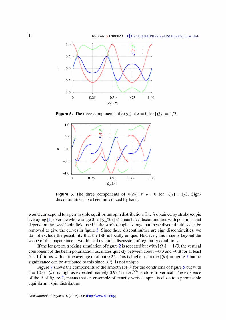
We now consider our first case of orbital resonance, namely with Q2 = 47 + 1/3, correspondingto odd a2 and b2. Figure 5 shows the components of n at δ = 0 and ε = 0.4. These componentsare obtained by normalizing to unity the �r(3) corresponding to three turns in the range0 < [φ2/2π] � 1/3, namely 0–120◦, and then transporting the n for each [φ2/2π] in this rangefor two or more turns with the 1-turn spin map, thereby filling up the full phase range. Notethat the curves are single valued functions of [φ2/2π] as required. The average |〈n〉| of n over[φ2/2π] in figure 5 is 0.05 and 〈n〉 is vertical. While the smooth ISF n of figure 5 is globallyunique, one loses global uniqueness if one allows discontinuities, as demonstrated in figure 6.There, we introduce changes of sign in n by hand at the arbitrarily chosen angles of 17.5 and90◦, while constructing n in the range 0–120◦ using �r(3). We then transport this n for two ormore turns as before. Naturally, the sign-discontinuities (often simply called ‘discontinuities’from now on) are transported too. In particular, we see that the transported n is still a singlevalued function of [φ2/2π]. The average |〈n〉| in figure 6 is 0.164. It is clear that neither n nor|〈n〉| are unique. Of course, an unlimited number of discontinuities could be introduced in thesame way. Then the curves would be smooth almost nowhere. Each of the n obtained in this way


http://www.njp.org/


–1.0

–0.5

0.0

0.5

1.0

0 0.25 0.50 0.75 1.00

n

[φ2/2π]

n1n2n3

Figure 5. The three components of n(φ2) at δ = 0 for [Q2] = 1/3.

–1.0

–0.5

0.0

0.5

1.0

0 0.25 0.50 0.75 1.00

n

[φ2/2π]

n1n2n3

Figure 6. The three components of n(φ2) at δ = 0 for [Q2] = 1/3. Sign-discontinuities have been introduced by hand.

would correspond to a permissible equilibrium spin distribution. The n obtained by stroboscopicaveraging [1] over the whole range 0 < [φ2/2π] � 1 can have discontinuities with positions thatdepend on the ‘seed’ spin field used in the stroboscopic average but these discontinuities can beremoved to give the curves in figure 5. Since these discontinuities are sign discontinuities, wedo not exclude the possibility that the ISF is locally unique. However, this issue is beyond thescope of this paper since it would lead us into a discussion of regularity conditions.

If the long-term tracking simulation of figure 2 is repeated but with [Q2] = 1/3, the verticalcomponent of the beam polarization oscillates quickly between about −0.3 and +0.8 for at least5 × 106 turns with a time average of about 0.25. This is higher than the |〈n〉| in figure 5 but nosignificance can be attributed to this since |〈n〉| is not unique.

Figure 7 shows the components of the smooth ISF n for the conditions of figure 5 but withδ = 10.6. |〈n〉| is high as expected, namely 0.997 since �r(3) is close to vertical. The existenceof the n of figure 7, means that an ensemble of exactly vertical spins is close to a permissibleequilibrium spin distribution.


http://www.njp.org/


–1.0

–0.5

0.0

0.5

1.0

0 0.25 0.50 0.75 1.00

n

[φ2/2π]

n1n2n3

Figure 7. The three components of n(φ2) at δ = 10.6 for [Q2] = 1/3.

–1.0

–0.5

0.0

0.5

1.0

–10 –8 –6 –4 –2 0 2 4 6 8 10

P2

δ

0.05 GeV p.t.0.30 GeV p.t.1.00 GeV p.t.

Figure 8. With each spin initially parallel to its n, the beam polarization, sampledturn-by-turn, for [Q2] = 1/3 during acceleration from δ = −10.6 to δ = +10.6at the rates of 50 MeV, 300 MeV and 1 GeV per turn.

Figure 8 shows the beam polarization for acceleration through δ = 0 from δ = −10.6 toδ = +10.6 at the rates of 50 MeV, 300 MeV and 1 GeV per turn for this Q2. At the start, theparticles are distributed uniformly in [φ2/2π] and the spins are set parallel to the almost verticaln vectors of the smooth ISF. Up to an acceleration rate of 50 MeV per turn, Js is invariant, withthe beam polarization dipping down to 0.05 around δ = 0 and returning to a high value at theend. This is a demonstration that with the chosen smooth n, Js can be adiabatically invariant,although the proof in [9] does not guarantee this because the system is on orbital resonance. Atthe higher acceleration rates, the invariance is lost. By using stroboscopic averaging for irrational[Q2] near 1/3 one finds ISFs similar to that in figure 5.

3.3. On orbital resonance: [Q2]=1/4

For our second case of orbital resonance we choose Q2 = 47 + 1/4, corresponding to an odda2 and a b2 which is twice an even integer. Figure 9 shows the components of n at δ = 0 and


http://www.njp.org/


–1.0

–0.5

0.0

0.5

1.0

0 0.25 0.50 0.75 1.00

n

[φ2/2π]

n1n2n3


ε = 0.4 obtained, in analogy with the previous case, from �r(4) in the range 0 < [φ2/2π] � 1/4and from transporting those n for three or more turns. In this case we see ‘stray’points at multiplesof 45◦ corresponding to the phases where the 4-turn map is the identity. For this figure we haveimposed the constraint that the components are continuous in the range 0–90◦, apart from thestray points. If we had not imposed smoothness, the components would have changed sign at 45◦

and the resulting discontinuities would have been transported to the remainder of the phase range.So, for these parameters and for [Q2] = 1/4, n can have discontinuities as in the case of anyrational Q2. But in contrast to a case discussed below, these discontinuities can be suppressed.The n obtained by stroboscopic averaging over the whole range 0 < [φ2/2π] � 1 is smooth asin figure 9. Of course, as in the case of [Q2] = 1/3, we can also introduce an unlimited numberof sign-discontinuities. The curves of figure 9 give |〈n〉| = 0.43. Note the similarity betweenfigure 9 and figure 1. Such similarities are seen with other irrational [Q2] near 1/4 and indicatea weak dependence of n on such irrational [Q2]. This is consistent with the prediction in ([4]subsection 4.8) that in mid-plane symmetric rings the ISF is well behaved close to the conditionν0 = k0 + 2k2Q2, (k0, k2 ∈ Z).

If the long-term tracking simulation of figure 2 is repeated but with [Q2] = 1/4, the verticalcomponent of the beam polarization oscillates quickly, initially between about −0.1 and +0.7.

But these limits gradually change and become 0.1 and 0.4 respectively after 5 × 106 turns. Thetime average is about 0.25. This is lower than the |〈n〉| in figure 9 but no significance can beattributed to this since |〈n〉| is not unique.

Figure 10 shows the components of n for the conditions of figure 9 but with δ = 10.6. Theaverage |〈n〉| is 0.99. Note that in contrast to the 3-turn map used for [Q2] = 1/3, at large δ

the 4-turn map is close to the identity. Nevertheless, �r(4) is close to vertical.Figure 11 shows the beam polarization as the simulation of figure 4 is repeated for

[Q2] = 1/4. At the start, the spins are set parallel to the almost vertical n vectors of the smoothISF. Up to an acceleration rate of 100 MeV per turn, Js is invariant, with the beam polarizationdipping down to 0.43 around δ = 0 and returning to a high value at the end. This is again ademonstration that with the chosen n, Js can be adiabatically invariant although the system is onorbital resonance. At the higher acceleration rates, the invariance is lost.


http://www.njp.org/


–1.0

–0.5

0.0

0.5

1.0

0 0.25 0.50 0.75 1.00

n

[φ2/2π]

n1n2n3


–1.0

–0.5

0.0

0.5

1.0

–10 –8 –6 –4 –2 0 2 4 6 8 10

P2

δ

0.10 GeV p.t.0.50 GeV p.t.1.00 GeV p.t.

Figure 11. With each spin initially parallel to its n, the beam polarization, sampledturn-by-turn, for [Q2] = 1/4 during acceleration from δ = −10.6 to δ = +10.6at the rates of 100 MeV, 500 MeV and 1 GeV per turn.

3.4. On orbital resonance: [Q2]=1/6

We now come to the first of the two cases of primary interest for this study, namely the case when[Q2] = 1/6, i.e. a case of a snake resonance. Again, the integer part of Q2 is 47 and ε = 0.4.Figure 12 shows the components of n at δ = 0 obtained by transporting for five or more turnsthe n obtained from �r(6) in the range 0 < [φ2/2π] � 1/6.

We see stray points at phases which are multiples of 30 and 90◦ corresponding to the phaseswhere the 6-turn map is the identity. The vector �r(6) has sign-discontinuities at these points butfor this figure we have imposed the constraint that the components of n are continuous in therange 0–60◦, apart from the stray points. One sees that n still has discontinuities, namely atphases which are multiples of 60◦. Thus, in spite of smoothing n in the initial range of 0–60◦,discontinuities persist. They cannot be removed without creating a vector field which becomesdouble valued when it is transported turn-by-turn. However, the discontinuities can be moved.These effects explain the failure of the MILES algorithm for n at snake-resonance tunes in [21]


http://www.njp.org/


–1.0

–0.5

0.0

0.5

1.0

0 1/6 1/3 1/2 2/3 5/6 1

n

[φ2/2π]

n1n2n3


where the need for discontinuities in this model is nevertheless disputed. It is clear that the curvesin figures 7 and 8 in [21] do not represent n [5].

Stroboscopic averaging over the whole range 0 < [φ2/2π] � 1 generates the curves offigure 12 directly, i.e. without extra smoothing. The discontinuities of n occur at phases wherethe raw stroboscopic average passes through zero. The passage through zero is smooth. Sodiscontinuities in n do not imply discontinuities in the stroboscopic average.

Our numerical calculations show that n has such discontinuities at snake-resonance tunesat most values of ε and that the minimum number of discontinuities is 2b2.

Of course, if n is represented as the locus of points on the unit 2-sphere, one finds disjointsegments. The average |〈n〉| over [φ2/2π] in figure 12 is 0.13. An arbitrary number of extradiscontinuities can be introduced by hand.

If the long-term tracking simulation of figure 2 is repeated but with [Q2] = 1/6, thepolarization oscillates quickly, but with constant upper and lower limits with a time averageof about 0.1, at least up to 5 × 106

turns. Thus the time averaged polarization does not vanish. This is illustrated in figure 13.

Figure 14 shows n obtained as for figure 12 but with δ = 10.6. Except when λ is an eveninteger this is typical of the n at large δ (and also at small ε). The value of �r(6) is very smalland the 6-turn spin map is close to a rotation of 2π around n. The discontinuities persist but incontrast to the earlier examples, the vertical component of n is close to zero and the horizontalcomponents are piece-wise almost independent of [φ2/2π]. The average |〈n(φ2)〉| is essentiallyzero. It would remain close to zero if sign-discontinuities were introduced by hand. Since thehorizontal components of n are piece-wise almost independent of [φ2/2π] but also different, andsince the 1-turn spin map is a rotation of about π around an axis close to the vertical, it essentiallychanges their signs from turn to turn, causing the discontinuities. Such discontinuities donot occur at large δ for [Q2] = 1/3 or [Q2] = 1/4 in figures 7 and 10 because n is close tovertical. The curves of figure 14 deform continuously into those of figure 12 as δ is reduced tozero. The analogous curves for the other three tunes show the same kind of behaviour and, ofcourse, that behaviour is a prerequisite for Js is to be invariant in figures 4, 8 and 11.

For [Q2] = 1/6 with ε = 0.4 and large non-even integer λ, all equilibrium spin distributionshave spins close to the horizontal plane. Thus a spin distribution in which all spins are initially


http://www.njp.org/


–100–80–60–40–20

020406080

100

0 1 2 3 4 5

P2

/%

Turns /106

Figure 13. For initially vertical spins, the vertical component of the beampolarization, sampled every 1000 turns, at δ = 0 for [Q2] = 1/6.

–1.0

–0.5

0.0

0.5

1.0

0 1/6 1/3 1/2 2/3 5/6 1

n

[φ2/2π]

n1n2n3


vertically upward cannot be in equilibrium. This is confirmed in figure 15 where we repeatthe long-term tracking simulation of figures 2 and 13 but at δ = −10.6 and [Q2] = 1/6. Wenow see that the polarization falls, but slowly, over many tens of thousands of turns andsubsequently oscillates around zero. Then the time averaged polarization is close to |〈n(φ2)〉| ≈ 0.Nevertheless, since the system is on orbital resonance, the theorem [3, 4] on the maximumtime averaged polarization does not enforce this. Although the initial spin distribution is notin equilibrium, it is not surprising that it takes about 105 turns before the polarization reacheszero. This is due to the fact that at large |δ| the eigentune, 6ν6, of the 6-turn spin map is almostindependent of [φ2/2π] and very close to an integer for this case. Since Js is invariant along atrajectory, we can view the motion of a spin as a precession at a fixed angle cos−1(�S · n/|�S|)around its n. In this case the angles are about 90◦. With eigentunes almost independent of [φ2/2π]and close to an integer, the projections of spins on the planes perpendicular to their respectiven’s spread out (decohere) only slowly. Then, at the viewing position, the spins return almost totheir original directions after six turns.


http://www.njp.org/


–100–80–60–40–20

020406080

100

0 1 2 3 4 5

P2

/%

Turns /106

Figure 15. For initially vertical spins, the vertical component of the beampolarization, sampled every 1000 turns, at δ = −10.6 for [Q2] = 1/6.

–0.1

–0.05

0.00

0.05

0.10

0.15

–10 –8 –6 –4 –2 0 2 4 6 8 10

P2

δ

50 keV p.t. 10 MeV p.t.

500 MeV p.t.

Figure 16. The beam polarization for [Q2] = 1/6 during acceleration fromδ = −10.6 to δ = +10.6 at the rates of 50 KeV, 10 MeV and 500 MeV per turnwith the spins initially parallel to n.

For large |δ|, the 1-turn spin map corresponds to a rotation of about π around an axis closeto the vertical. So, it is again no surprise that the polarization in figure 15 takes many turns toreach zero. For even larger δ (e.g. over 100), n can be taken to be horizontal but the polarizationremains vertical and it takes many millions of turns for it to show signs of falling. There is nofall if λ is an even integer since then, the 6-turn map is the identity.

Figure 16 shows the beam polarization for acceleration through δ = 0 at the rates of 50 KeV,10 MeV and 500 MeV per turn for [Q2] = 1/6.At the start, the particles are uniformly distributedin [φ/2π] and the spins are set parallel to the almost horizontal n vectors of that ISF which deformsinto the ISFs of figures 12 and 14. The initial beam polarization is essentially zero. Duringacceleration at rates up to 50 KeV per turn, the beam polarization rises to 0.13, correspondingto the |〈n〉| of figure 12, and then returns to around zero. A detailed inspection of the data showsthat for a rate of 10 MeV per turn, the spins deviate slightly from their respective n vectors


http://www.njp.org/


0

0.2

0.4

0.6

0.8

1.0

–10 –8 –6 –4 –2 0 2 4 6 8 10

⟨ |J s

|⟩

δ

50 keV p.t. 10 MeV p.t.500 MeV p.t.

Figure 17. With each spin initially parallel to its n, 〈Js〉 during acceleration fromδ = −10.6 to δ = +10.6 at the rates of 50 KeV, 10 MeV and 500 MeV per turnwith [Q2] = 1/6.

–1.0

–0.5

0.0

0.5

1.0

–10 –8 –6 –4 –2 0 2 4 6 8 10

P2

δ

50 keV p.t.10 MeV p.t.50 MeV p.t.

Figure 18. For initially vertical spins, the beam polarization for [Q2] = 1/6during acceleration from δ = −10.6 to δ = +10.6 at the rates of 50 KeV, 10 MeVand 50 MeV per turn.

at large δ. However, this effect is not apparent in the average over [φ2/2π] contained in thebeam polarization. This is again a demonstration that with the chosen n and the chosen layoutof accelerating cavities, Js can be approximately invariant even for these discontinuous ISFsand that at the higher acceleration rates, the invariance is lost. The approximate invariance isconfirmed in figure 17 which shows the corresponding behaviour of the phase average of Js,〈Js〉. In figure 17 we have suppressed data at δ’s where n is indeterminate because λ is an eveninteger.

Figure 18 shows the beam polarization as the simulation of figure 16 is repeated but with thespins initially vertically upward and for rates of 50 KeV and 10 MeV per turn and for 50 MeV perturn, where Js is still approximately invariant. For these rates of acceleration the angle between aspin and its n remains around 90◦. Then the beam polarization during acceleration depends juston the geometry of the ISF and on the history of the rate of decoherence of the projections of


http://www.njp.org/


–100–80–60–40–20

020406080

100

0 1 2 3 4 5

P2

/%

Turns /106

50 keV p.t.10 MeV p.t.50 MeV p.t.

Figure 19. The beam polarization for [Q2] = 1/6 when δ is frozen at +10.6after the acceleration cycle of figure 18, and the spins are tracked for a further5 × 106 turns.

the spins on the planes perpendicular to the n’s. These rates depend, in turn, on the magnitudeof 6ν6 and its dependence on [φ2/2π]. We therefore expect that the final polarization coulddepend sensitively on the magnitude of the rate of acceleration and on its time dependence.This is confirmed in figure 18 which shows that at a rate of 50 KeV per turn, the polarizationis effectively lost at positive δ but that at the much higher rate of 50 MeV per turn the finalpolarization is around −0.4 at the end of the acceleration cycle. By now, the reader will haverealized that the polarization of −0.4 cannot represent an equilibrium state. This is confirmedin figure 19 where, after acceleration up to δ = 10.6, δ is frozen and the ensembles are trackedfor a further 5 × 106 turns. Figure 19 shows that after some large oscillations the polarizationgradually decays to zero in a way and on a time scale familiar from figure 15. It also showsthat although the polarization can be small at the end of the acceleration (as in the case of10 MeV/turn), the spin distribution is by no means isotropic but is such that the polarization canreturn to a large value later. In fact after the 5 × 106 turns, the curves of spin vector versus [φ2/2π]are smooth curves for all three acceleration rates5. This suggests that contrary to conventionalexpectation, a complete loss of polarization is not inevitable during acceleration exactly at a snakeresonance with [Q2] = 1/6, at least not within the confines of our model. This completes Part I ofour investigation.

4. Summary and conclusion

In this paper, we have presented and contrasted four scenarios for spin motion on and off orbitalresonance within the confines of our simple model, and by this means we have developed a clean,elegant account of the special features of spin motion at a snake resonance. In all four cases�S · n is an invariant at low enough rates of acceleration. For the first three cases ([Q2] =0.236067977 . . . , 1/3, 1/4) the ISF is close to vertical at large |δ|, i.e. far away from the energyfor the parent resonance, and the spin motion is unexceptional. For example, after acceleration

5 This vindicates the advice in ([7] section I) on the use of the term ‘depolarization’.


http://www.njp.org/


from a large negative δ to a high positive δ, an initially vertical spin is still close to vertical.These cases serve to emphasize the exceptional form of the ISF when [Q2] = 1/6. In this case,far away from the parent resonance, the ISF lies close to the horizontal plane. Then in contrast tothe other three cases, an ensemble of particles with a uniform distribution of [φ2/2π] and withvertically upward spins, cannot be at spin equilibrium. The subsequent evolution of the beampolarization depends on the chosen initial δ and is exemplified in figures 13 and 15. In particular,the polarization oscillates at a rate depending on the proximity of the eigentune of the 6-turn spinmap to an integer and on the extent of the variation of that eigentune with [φ2/2π]. Then at theenergy of the parent resonance (δ = 0), the polarization oscillates quickly and the time averagedpolarization is small but nonzero. At most large |δ|, the time averaged polarization is zero butthe polarization oscillates slowly and it reaches zero for the first time only after many thousandsof turns.

As soon as one sees that at most large δ the ISF for [Q2] = 1/6 lies close to the horizontalplane, it is no surprise that in this case the time averaged beam polarization can become small inthe long term.Acceleration adds little to the story, except that within our model, after starting withan ensemble of vertical spins at δ = −10.6, the final polarization depends on the rate at whichone passes from the spin motion underlying figure 15 to the spin motion underlying figure 13and then beyond to large positive δ. The key features of spin motion at [Q2] = 1/6 are encodedin the ISF. We see no necessity to invoke the perturbed spin tune [14, 15]. Instead, we appeal tothe eigentune of the 6-turn spin map, a quantity with physical significance.

We emphasize that the main results presented here refer to a very special case, namelyfor our model right at [Q2] = 1/6 and with ε = 0.4. As pointed out in [5], the ISF is extremelycomplicated for values of [Q2] just below and just above 1/6. This is consistent with the predictionin ([4] subsection 4.8) that in mid-plane symmetric rings the ISF need not be well behaved closeto the condition ν0 = k0 + (2k2 + 1)Q2, (k0, k2 ∈ Z). Thus in Part II of this study we extend ourcalculations to cover such values of [Q2] and to larger values of ε. It will be shown there thatalthough the ISF for [Q2] = 1/6 has the special form described above, this is an exception andthat the loss of polarization during acceleration near to [Q2] = 1/6 has a different origin. Wealso comment on the findings in [10, 23, 24].

The analysis should then be extended to real synchrobetatron motion with misalignmentsfor a typical optic of a real ring and with the fields of real snakes. See, for example, [33]. Othersnake-resonance tunes should also be covered. We note with interest that according to simulationsfor RHIC, the loss of polarization during acceleration is less severe when the simulations arecarried out with the magnetic fields of real snakes rather than with point-like snakes [34].

Acknowledgments

We thank K Heinemann, G H Hoffstaetter and J A Ellison for useful discussions and for valuedcollaboration and we thank L Malysheva for help during the preparation of this paper.

References

[1] Heinemann K and Hoffstaetter G H 1996 Phys. Rev. E 54 4240[2] Hoffstaetter G H, Vogt M and Barber D P 1999 Phys. Rev. ST Accel. Beams 11 114001[3] Hoffstaetter G H 2006 High Energy Polarized Proton Beams: A Modern View (Springer Tracts in Modern

Physics Vol 218) (Berlin: Springer)


http://dx.doi.org/10.1103/PhysRevE.54.4240

http://dx.doi.org/10.1103/PhysRevSTAB.2.114001

http://www.njp.org/


[4] Vogt M 2000 PhD Thesis University of Hamburg, DESY-THESIS-2000-054[5] Barber D P, Jaganathan R and Vogt M 2003 Proc. 15th Int. Spin Physics Symp. (Brookhaven National

Laboratory, Long Island, NY, September 2002) AIP Proc. 675Barber D P, Jaganathan R and Vogt M 2005 Extended version: Preprint physics/0502121

[6] Hoffstaetter G H and Vogt M 2004 Phys. Rev. E 70 056501[7] Barber D P, Ellison J A and Heinemann K 2004 Phys. Rev. ST Accel. Beams 7 124002[8] Barber D P, Ellison J A and Heinemann K 2005 Phys. Rev. ST Accel. Beams 8 089002[9] Hoffstaetter G H, Dumas H S and Ellison J A 2006 Phys. Rev. ST Accel. Beams 9 014001

[10] Yokoya K 1988 SSC CDG Report SSC-189[11] Derbenev Ya S and Kondratenko A 1976 Sov. Phys.—Dokl. 20 562[12] Derbenev Ya S et al 1978 Part. Accelerators 8 115[13] Lee S Y and Tepikian S 1986 Phys. Rev. Lett. 56 1653[14] Lee S Y 1989 Proc. 8th Int. Symp. on High Energy Spin Physics (Minneapolis, MN, September 1988) AIP

Proc. 187[15] Lee S Y 1997 Spin Dynamics and Snakes in Synchrotrons (Singapore: World Scientific)[16] Luccio A 1995 Brookhaven National Laboratory Technical Report BNL-52481[17] Ptitsyn V et al 2005 Proc. 16th Int. Spin Physics Symp. (Trieste, October 2004) (Singapore: World Scientific)[18] Bai M et al 2005 Proc. 16th Int. Spin Physics Symp. (Trieste, Italy, October 2004) (Singapore: World Scientific)[19] Ptitsin V I 1997 PhD Thesis Budker Institute of Nuclear Physics, Novosibirsk (in Russian)[20] Ptitsin V I 1997 Proc. 12th Int. Symp. on High Energy Spin Physics (Amsterdam, September 1996) (Singapore:

World Scientific)[21] Mane S R 2004 Nucl. Instrum. Methods A 528 667[22] Lee S Y and Mane S R 2005 Phys. Rev. ST Accel. Beams 8 089001[23] Buon J 1986 Proc. Workshop on Polarized Beams at the SSC (Ann Arbor, MI, 1985) AIP Proc. 145[24] Ptitsin V I 1995 AGS/AD Technical Note 419, Brookhaven National Laboratory, NY[25] Froissart M and Stora R 1960 Nucl. Instrum. Methods 7 297[26] Yokoya K 1999 DESY Report 99-006 (Preprint physics/9902068)[27] Jackson J D 1998 Classical Electrodynamics 3rd edn (New York: Wiley)[28] Barber D P, Heinemann K and Ripken G 1994 Z. Phys. C 64 117[29] Lee S Y 2006 Phys. Rev. ST Accel. Beams 9 074001[30] Mane S R 1988 Fermilab Technical Report TM-1515[31] Mane S R 2002 Nucl. Instrum. Methods A 480 328

Mane S R 2002 Nucl. Instrum. Methods A 485 277[32] Hamilton W R 1844 Proc. R. Irish Acad. 2 424[33] Ranjbar V H et al 2003 Phys. Rev. Lett. 91 034801[34] Xiao M and Katayama T 2003 University of Tokyo Technical Report CNS-REP-51


http://dx.doi.org/10.1103/PhysRevE.70.056501




http://dx.doi.org/10.1016/j.nima.2004.03.208


http://dx.doi.org/10.1016/0029-554X(60)90033-1

http://dx.doi.org/10.1007/BF01557243


http://dx.doi.org/10.1016/S0168-9002(01)00955-X

http://dx.doi.org/10.1016/S0168-9002(01)02140-4

http://dx.doi.org/10.1103/PhysRevLett.91.034801

http://www.njp.org/

spin motion at and near orbital resonance in storage rings

Documents