spherical and ring-like configurations for the ... · introduction the jefimenko’s equations...

Open Access Journal of Physics

Volume 2, Issue 1, 2018, PP 1-12

Open Access Journal of Physics V2● 11 ● 2018 1

Spherical and Ring-Like Configurations for the

Gravitodynamical Field

David Perez-Carlos, Augusto Espinoza and Andrew Chubykalo

Academic Unit of Physics. Autonomous University of Zacatecas, Zacatecas, Mexico

*Corresponding Author: David Perez-Carlos, Academic Unit of Physics. Autonomous University of Zacatecas, Zacatecas, Mexico.

INTRODUCTION

The Jefimenko’s equations arise from an

analogy between the laws that rules the electrodynamics and the laws of gravitation.

Such analogy was proposed for the first time by

Heaviside in a paper published [1] more than a century ago, where he supposed there must exist

a second field due to moving masses and acting

over moving masses only, called by Jefimenko, cogravitational field (sometimes this field is

called Heaviside’s field). The Heaviside paper

was forgotten for a long time until Jefimenko

returned his work and made improvement to the Heaviside’s work in two books published and

reissued since the 90’s decade [2], [3].

To start we need to write about the analogy made by Jefimenko between the laws of

electromagnetism and the laws of gravitation.

Oliver Heaviside proposed a system of

equations with the same structure as the Maxwell’s equations, assuming the existence of

a second field due and acting over moving

masses only, called Heaviside’s field or co

gravitational field and it is denoted by 𝐤, unlike

the ordinary gravitational field 𝐠 which is due

and acts not only on stationary masses but in movement. Although there are detractors of the

Jefimenko’s theory of gravitation1 (see for

example [5]), there exist books written by

Wenceslao Segura [6] and Jolien E. D. Creighton [7] where they derived the Jefimenko’s equations

from the linearized Einstein’s equations. Jefimenko

derived the equations of gravitodynamics in a different way, starting from make an analogy of

his retarded solutions of the electromagnetic

field to the gravitodynamical field to finally get the analogous equations to the Maxwell’s

equations for the gravitational and cogravitational

fields.

Next, we assume there is a configuration of the gravitodynamical field in an analogue way to

those found in other works realized by

Chubykalo and Espinoza [8], [9], where the authors have obtained the mathematical

foundations on the Kapitsa’s hypothesis [10]

about the origin of ball lightning related with

interference processes. The configuration of the gravitodynamical field in our work begins with

1Called by us in a previous work gravitodynamical

theory [4].

ABSTRACT

In the present work, we write a brief exposition of the Jefimenko’s theory of gravitation. This theory arose

from the analogy between the laws of gravitation and electromagnetism, that is, exist a second gravitational

field called cogravitational field, analogous to the magnetic field. We introduce a new system of units called

Gravitational Gaussian System (GGS). This system allows us write the equations of gravitation in a simple

form to solve them. Using the Jefimenko’s equations of gravitation, we obtain the wave equations for

gravitational and cogravitational fields and we find wave solutions. We demonstrate there are

configurations of the gravitodynamical field (that is, the set of gravitational and cogravitacional fields) in

form of co gravitational field spheres and gravitational field rings. This phenomenon must be an analogue of

the ball lightning in the electromagnetic field, but in this case the cogravitational field spheres serves as

containers of matter (it could be a gas). We analyze how this configuration acts on the particles inside the spheres, and we investigate the physical properties of such configurations, namely, how behaves the density

of energy and the Pointing vector of this solution.

Keywords: Cogravitation; Gravitational waves; Gravitodynamical field.

PACS: 04.50.Kd; 04.30.-w

Spherical and Ring-Like Configurations for the Gravitodynamical Field

2 Open Access Journal of Physics V2● 11 ● 2018

the hypothesis that the gravitational waves exist.

We are going to do a formal development about this issue based in the theoretical results

obtained by Jefimenko. We will use the free

gravitodynamical equations, that is, the equations valid for vacuum.

It is important to emphasize that gravitational

waves were predicted in the general theory of

relativity by linearzing Einstein's field equations and this approximation is valid for weak fields.

It is obvious that a complete theory of gravity is

not linear but this linear approximation allows us to study a great variety of gravitational

phenomena where gravitational induction is

considered. In the same way that electromagnetic theory is not linear but Maxwell

equations are applicable to a wide range of

electromagnetic phenomena.

Our results presented here do not try to replace the non-linear theories of gravitation, such as

Einstein’s theory of general relativity [11] or

Logunov’s relativistic theory of gravitation [12], but we want to show the importance of a linear

gravitational theory, not only historical but

methodological too, because we will show that

exist properties of the weak fields that are not understood because they were not have the

opportunity to appear in a linear theory of

gravitation.

THE JEFIMENKO’S EQUATIONS FOR

GRAVITATION

The gravitodynamical theory is a generalization

of the Newton’s gravitation theory, since the

Newtonian theory of gravitation describes perfectly phenomena of a wide range of masses,

but it does not consider the behavior of the

fields of moving mass distributions. This is the reason why it is necessary to make an extension

of the classical Newton’s theory of gravitation.

We can write the Newton’s theory in a way as a

force field theory in terms of the gravitational

field 𝐠 as

∇ ∙ 𝐠 = −4𝜋𝛾𝜚 (1)

and

∇ × 𝐠 = 0, (2)

where 𝛾 is the gravitational constant, 𝜚 is the

mass density given by 𝜚 = 𝑑𝑚/𝑑𝑉 and 𝑑𝑚 is

the element of mass contained in the volume

element 𝑑𝑉.

As we know, the gravitational field 𝐠 is defined

by means of the force exerted by the mass

distribution 𝜚 over a mass test

𝐅𝘨 = 𝑚𝑡𝐠. (3)

In other words, the gravitational field is the

perturbation of the space due to distribution of

mass in some region which interact on a test

mass 𝑚𝑡 Both masses (the mass creating the

field and the test mass) can be moving or at rest.

If we consider that the co gravitational field 𝐤

exists, we need to define it in terms of the co gravitational force

𝐅𝑘 = 𝑚𝑡 𝐯 × 𝐤 , (4)

Where 𝐅𝑘 is the force exerted by the

cogravitational field over a test mass 𝑚𝑡 moving

with velocity 𝐯.

So, we can define the cogravitational field 𝐤 as

the perturbation of the space due to a moving

mass distribution which interacts on a moving test mass.

Jefimenko started to derive their gravitational

equations from the next expressions

𝐠 = −𝛾 [𝜚]

𝑟3+

1

𝑟2𝑐 𝜕𝜚

𝜕𝑡 𝐫𝑑𝑉 ′ +

𝛾

𝑐2

1

𝑟 𝜕 𝜚𝐯

𝜕𝑡 𝑑𝑉 ′ (5)

and

𝐤 = −𝛾

𝑐2

[𝜚𝐯]

𝑟3+

1

𝑟2𝑐 𝜕(𝜚𝐯)

𝜕𝑡 × 𝐫𝑑𝑉 ′, (6)

where 𝛾 is the gravitational constant, 𝑐 is the

velocity of propagation of the fields2 and 𝐫 is the

vector directed from the element of volume 𝑑𝑉 ′ (the source point) to the point where the

gravitodynamical field is measured (the field

point) and 𝑟 is its magnitude, the square

brackets designate that the quantities inside

them are evaluated in the delayed time𝑡′ = 𝑡 −𝑟/𝑐. The integrals are evaluated over all space.

We can see from (5) and (6) that the gravitodynamical fields have four causative

sources, namely: the mass density 𝜚, the

temporal derivative of the mass density 𝜕𝑡𝜚, the

mass current 𝜚𝐯and its time derivative 𝜕𝑡(𝜚𝐯).

Jefimenko obtained the gravitodynamical

equations making use of the vector calculus and

some vector identities. The gravitodynamical

equations are:

∇ ∙ 𝐠 = −4𝜋𝛾𝜚, (7)

∇ ∙ 𝐤 = 0, (8)

∇ × 𝐠 = −𝜕𝐤

𝜕𝑡, (9)

2Jefimenko assumed that the velocity of the

propagation of the fields must be 𝑐, i.e, the finite

speed of light. But we have demonstrated in [4] that

this velocity must be finite or instantaneous.



∇ × 𝐤 −

1

𝑐2

𝜕𝐠

𝜕𝑡= −

4𝜋𝛾

𝑐2𝐣, (10)

where j= 𝜚𝐯 is the mass current density. It is

evident the analogy between the Maxwell equations and the Jefimenko’s ones is not

perfect: while we have only one kind of mass,

we have two types of electric charge. While the electric field is directed from the positive

charges that generate it and is directed toward

negative charges, the gravitational field is always directed to the masses by which it is

created. Another difference is that the magnetic

field is dextrorotatory (right hand) with respect

to the electric current through which it is generated, while the gravitational field is always

levorotatory (left hand) with respect to the mass

current through which it is generated. In spite of these differences, the system of equations

obtained by Jefimenko describe correctly the

behavior of the weak gravitational fields, as we

have already seen they are deduced from different formulations in [3] and in [6], [7].

We define a Gaussian system of units for the

gravitodynamical field, in order to simplify our calculations. We will call this system

Gravitational Gaussian System (GGS).To do

this we need to introduce the next rationalized quantities:

Table1. Rationalized quantities in the new gravitational

Gaussian system of units3.

Gravitational field Co gravitational field

Formula 𝐆 = 𝛾−1𝐠 𝐊 = 𝛾−1𝑐𝐤

Units 𝐆 = 𝑀𝐿−2 =Jef 𝐊 = 𝑀𝐿−2 =Jef

If we introduce such quantities in the system of

Equations (7)-(10) we obtain the next system of

equations in the GGS

∇ ∙ 𝐆 = −4𝜋𝜚, (11)

∇ ∙ 𝐊 = 0, (12)

∇ × 𝐆 = −1

𝑐

𝜕𝐊

𝜕𝑡, (13)

∇ × 𝐊 −1

𝑐

𝜕𝐆

𝜕𝑡= −

4𝜋

𝑐𝐣. (14)

Where, 𝐣 = 𝜚𝐯is the mass current density and

𝐯is the velocity of the mass distribution

generating the co gravitational field.

GRAVITATIONAL WAVES

The Jefimenko’s theory of gravitation predicts also the existence of gravitational waves. We

3We define the unit 𝐽efimenko abbreviated 𝐽ef for the

rationalized gravitational and co gravitational fields

in honor of Jefimenko.

will study the properties of such waves, in this

and in other sections (especially in the section V, where we will study the energy and the

Poynting vector of such waves).

We will obtain in this section the wave equation for both fields, namely, the gravitational field

and the cogravitational one, making direct

calculations on the system of equations (11)-(14), we will see that these equations lead us to

the wave equation. We start calculating the curl

on the equation (13)

∇ × ∇ × 𝐆 = −1

𝑐

𝜕

𝜕𝑡∇ × 𝐊, (15)

and substituting in equation (14) and using the identity for a Laplacian of a vector,

∇ × ∇ × 𝐕 = 𝛁 𝛁 ∙ 𝐕 − ∆𝐕, (16)

for any arbitrary vector 𝐕, and where ∆= ∇2is

the Laplacian operator, we get

∆𝐆 −1

𝑐2

𝜕2𝐆

𝜕𝑡2= −4𝜋 ∇𝜚 +

1

𝑐2

𝜕𝐣

𝜕𝑡 , (17)

the in homogeneous gravitational wave

equation.

In a similar way, starting from (14) taking the

curl and using the identity (16), we get

∆𝐊 −1

𝑐2

𝜕2𝐊

𝜕𝑡2=

4𝜋

𝑐∇ × 𝐣, (18)

Is the inhomogeneous cogravitational wave

equation. Both expressions (17) and (18) are

field waves propagating on the space with a

velocity 𝑐.

If we consider regions without masses

distributions and current masses we obtain the

homogeneous wave equations, namely,

∆𝐆 −1

𝑐2

𝜕2𝐆

𝜕𝑡2= 0 (19)

And

∆𝐊 −1

𝑐2

𝜕2𝐊

𝜕𝑡2= 0. (20)

The equations obtained (19) and (20) can be

solved by a sum of two vector functions, 𝝋1

and 𝝋2,

𝝋1 𝒌 ∙ 𝐫 − 𝜔𝑡 + 𝝋2 𝒌 ∙ 𝐫 + 𝜔𝑡 , (21)

Where 𝒌 = (𝑘𝑥 , 𝑘𝑦 , 𝑘𝑧) is the wave vector4, 𝝋1

and 𝝋2 are general expressions which represent

plane waves propagating with velocity 𝑐 in

4 To avoid confusions, we use italic boldface 𝒌 to

represent the wave vector and normal boldface 𝐤 to

represent the cogravitational field.



opposite directions. Then the solution (21) for

the wave equation can be derived from the method of separation of variables. If we

introduce the harmonic dependence given by

𝐆 = 𝐺0𝑒𝑖 𝒌∙𝐫±𝜔𝑡 𝒏𝐆 (22)

and

K = 𝐾0𝑒𝑖 𝒌∙𝐫±𝜔𝑡 𝒏𝐊, (23)

Where 𝒏𝐆 is a unitary vector in the direction of

propagation of 𝐆 and 𝒏𝐊 is in the direction of

propagation of 𝐊, the wave’s equation results in

the dispersion’s relation

𝜔2 − 𝑘2𝑐2 = 0. (24)

For the election of sign 𝑘 = + 𝜔 𝑐 , we obtain

from the Jefimenko’s equations for gravitodynamical fields

𝒌 ∙ 𝒏𝐆 = 0 and 𝙜 ∙ 𝒏𝐊 = 0, (25)

𝒌 × 𝒏𝐆 𝐺0 =𝜔

𝑐𝐾0𝒏𝐊 and 𝒌 × 𝒏𝐊 𝐾0

=𝜔

𝑐𝐺0𝒏𝐆. (26)

From Eq s. (25) And (26) we can see that 𝐆 and

𝐊 are vector mutually perpendicular to the

direction of propagation and 𝐺0 = 𝐾0 .

An Interesting Wave Solution of the

Jefimenko’s Equations for the Free Space

The prediction of gravitational waves by means

of the Jefimenko’s gravitodynamical theory let

us search a various types of solutions for the

gravitodynamical field in vacuum. For example,

as we will show in this section, solutions exist

that have a set of interesting properties. These

solutions have the form of spheres of co

gravitational field and ring-like gravitational

field, in such way the total configuration of the

gravitodynamical field oscillates. In such

spheres the Heaviside’s field is tangent in all

points over the surface of this sphere, and the

same for the ring-like configuration of the

gravitational field.

We will begin this section rewriting the

Jefimenko’s equations for the gravitation, assuming there are regions of free space or

vacuum, this means, 𝜚 = 0 and 𝐣 = 0. We get

∇ ∙ 𝐆 = 0, (27)

∇ ∙ 𝐊 = 0, (28)

∇ × 𝐆 = −1

𝑐

𝜕𝐊

𝜕𝑡, (29)

∇ × 𝐊 =1

𝑐

𝜕𝐆

𝜕𝑡. (30)

In Electrodynamics is usual to refer to standard polarity in the solutions of the Maxwell

equations when the electric field 𝐄 is a polar

vector and the magnetic induction B is an axial

vector, or pseudo-vector. This means that after a transformation of inversion of axis coordinates,

𝐄 changes its signs, while B maintains its signs.

Following the analogy between both theories we are going to look for solutions to these equations

with standard polarity, to wit, when the vector

𝐆 is polarand 𝐊 is axial. We propose to solve the

system of free Jefimenko’s equations by the method of separation of variables, we can write

𝐆 and 𝐊 as follows:

𝐆 𝐫, 𝑡 = 𝛄 𝐫 𝜇 𝑡 (31)

and

𝐊 𝐫, 𝑡 = 𝛋 𝐫 𝜈 𝑡 , (32)

where 𝛄 𝐫 is a polar vector and 𝛋 𝐫 is an

axial one, also 𝜇 𝑡 and 𝜈 𝑡 are functions of

time.

Substituting (31) and (32) in the system (27)-

(30)

∇ ∙ 𝛄 𝐫 = 0, (33)

∇ ∙ 𝛋 𝐫 = 0, (34)

∇ × 𝛄 𝐫 = −1

𝑐

1

𝜇 𝑡

𝜕𝜈 𝑡

𝜕𝑡𝛋 𝐫 , (35)

∇ × 𝛋 𝐫 =1

𝑐

1

𝜈 𝑡

𝜕𝜇 𝑡

𝜕𝑡𝛄 𝐫 . (36)

We can equate the temporal parts of both

equations to certain constants to obtain a consistent system,

−1

𝜇 𝑡

𝜕𝜈 𝑡

𝜕𝑡= 𝜔1 (37)

And

1

𝜈 𝑡

𝜕𝜇 𝑡

𝜕𝑡= 𝜔2 . (38)

We are going to equating both equations to 𝜔, in

order to obtain sinusoidal solutions and get only three constants in our system (37)-(38)

𝜈 𝑡 = 𝐴 cos 𝜔𝑡 − 𝛿 (39)

and

𝜇 𝑡 = 𝐴 sin 𝜔𝑡 − 𝛿 , (40)

where, 𝐴 and 𝛿 are arbitrary constants.



Thus, in this way, the equations for 𝛄 and

𝛋 become

∇ × 𝛄 𝐫 =𝜔

𝑐𝛋 𝐫 , (41)

and

∇ × 𝛋 𝐫 =𝜔

𝑐𝛄 𝐫 . (42)

Due to the linearity of the spatial components of

the fields, we can add (41) and (42), then, we

can define the vector

𝛔 𝐫 = 𝛄 𝐫 + 𝛋 𝐫 , (43)

Such as, we obtain

∇ × 𝛔 𝐫 =𝜔

𝑐𝛔 𝐫 . (44)

First of all, we are going to solve (44), then,

once we have obtained 𝛔, we can calculate

𝛄 and 𝛋. We need to note that vector 𝛔 has not

polarity, but we can express its polar and axial

parts as

𝛄 𝐫 =1

2 𝛔 𝐫 − 𝛔 −𝐫 (45)

And

𝛋 𝐫 =1

2 𝛔 𝐫 + 𝛔 −𝐫 . (46)

Taking the curl of (45) and (46), and inverting the coordinates of equation (44), we have

∇ × 𝛄 𝐫 =1

2 ∇ × 𝛔 𝐫 − ∇ × 𝛔 −𝐫

=1

2 𝜔

𝑐𝛔 𝐫 +

𝜔

𝑐𝛔 −𝐫

=𝜔

𝑐𝛋 𝐫 (47)

And

∇ × 𝛋 𝐫 =1

2 ∇ × 𝛔 𝐫 + ∇ × 𝛔 −𝐫 =

1

2 𝜔

𝑐𝛔 𝐫 −

𝜔

𝑐𝛔 −𝐫 =

𝜔

𝑐𝛄 𝐫 , (48)

we can be sure that the system is satisfied. The only thing we need to do is to find the solution

of (44), in order to find the solution of the

system (41)-(42). To get such solution we will

consider the vector 𝛔 in spherical coordinates

and we suppose that the solution has axial

symmetry

𝛔 = 𝜎𝒓 𝑟, 𝜃 𝒓 + 𝜎𝜃 𝑟, 𝜃 𝜽 + 𝜎𝜙 𝑟, 𝜃 𝝋 . (49)

The curl of 𝛔 in spherical coordinates is

∇ × 𝛔 =1

𝑟2 sin𝜃 𝜕 𝑟𝜎𝜙 sin 𝜃

𝜕𝜃−

𝜕 𝑟𝜎𝜃

𝜕𝜙 𝒓 +

1

𝑟 sin𝜃 𝜕 𝜎𝑟

𝜕𝜙−

𝜕 𝑟𝜎𝜙 sin 𝜃

𝜕𝑟 𝜽 +

1

𝑟 𝜕 𝑟𝜎𝜃

𝜕𝑟−

𝜕 𝜎𝑟

𝜕𝜃 𝝋 , (50)

We can obtain the next system of equations taking into account Eq. (44) and comparing it

with (49) and (50)

𝜕 𝜎𝜙 sin 𝜃

𝜕𝜃=

𝜔𝑟𝜎𝑟 sin 𝜃

𝑐, 51

𝜕(𝑟𝜎𝜙 )

𝜕𝑟= −

𝜔𝑟𝜎𝜃

𝑐 (52)

and

𝜕 𝑟𝜎𝜃

𝜕𝑟−

𝜕 𝜎𝑟

𝜕𝜃=

𝜔𝑟𝜎𝜙

𝑐. (53)

Expressing the variables 𝜎𝑟y 𝜎𝜃 from (51) y (52)

and replacing them in (53), we obtain the next

partial differential equation for 𝜎𝜙 , namely,

𝑟𝜕2

𝜕𝑟2 𝑟𝜎𝜙 +

𝜕

𝜕𝜃

1

sin 𝜃

𝜕

𝜕𝜃 𝜎𝜙 sin𝜃 +

𝜔2𝑟2

𝑐2𝜎𝜙

= 0. (54)

If we propose 𝜎𝜙 = 𝑅(𝑟)Θ(𝜃) as a solution for

(54) we find that 𝑅 and Θ have to satisfy

𝑟2𝑑2(𝑟𝑅)

𝑑𝑟2+

𝜔2𝑟2

𝑐2+ 𝜆 𝑟𝑅 = 0 (55)

And

𝑑

𝑑𝜃

1

sin 𝜃

𝑑

𝑑𝜃 Θ sin 𝜃 − 𝜆Θ = 0, (56)

where 𝜆 is an arbitrary constant? If 𝜆 = 0, then

the solution for 𝑟𝑅 in Equation (55) must be

𝐴 cos𝜔𝑟

𝑐+ 𝐵 sin

𝜔𝑟

𝑐, where 𝐴 and 𝐵 are

constants, but, in general, 𝐴 and 𝐵 depend on 𝑟, so

𝑟𝑅 = 𝐴 𝑟 cos𝜔𝑟

𝑐+ 𝐵 𝑟 sin

𝜔𝑟

𝑐. (57)

Now, we are going to substitute (57) in (55) and we obtain the next two equations

𝑑2𝐴

𝑑𝑟2+

𝜆

𝑟2𝐴 +

2𝜔

𝑐

𝑑𝐵

𝑑𝑟= 0 (58)

And

𝑑2𝐵

𝑑𝑟2+

𝜆

𝑟2𝐵 −

2𝜔

𝑐

𝑑𝐴

𝑑𝑟= 0, (59)

Considering the fact that the coefficients of sine

and cosine must be zero separately, due these functions has the same argument.

To solve (58) and (59) we propose 𝐴 𝑟 = 𝑎𝑟𝑚

and𝐵 𝑟 = 𝑏𝑟𝑛 , where the coefficients 𝑎 and 𝑏

are constants and 𝑛, 𝑚 ∈ 𝑁 are constants, too. Then, we obtain the following characteristic

equations, substituting the solutions proposed in

Eqs. (58) and (59)



𝑎𝑚 𝑚 − 1 + 𝜆𝑎 +2𝜔

𝑐𝑏𝑛𝑟𝑛−𝑚+1 = 0 (60)

and

𝑏𝑛 𝑛 − 1 + 𝜆𝑏 −2𝜔

𝑐𝑎𝑚𝑟𝑚−𝑛+1 = 0. (61)

Both equations can be satisfied for the next two cases:

Case1) 𝑚 = 0, 𝑛 = −1, 𝜆 = −2 and 𝑎 =−𝜔𝑏/𝑐, and regarding Eq. (57) for 𝑏 = 1, we obtain

𝑅 =1

𝑟2 −

𝜔𝑟

𝑐cos

𝜔𝑟

𝑐+ sin

𝜔𝑟

𝑐 ; (62)

Case2)𝑚 = −1, 𝑛 = 0, 𝜆 = −2 and 𝑏 = −𝜔𝑎/𝑐, and regarding Eq. (57) for 𝑎 = 1, we obtain,

𝑅 =1

𝑟2 cos

𝜔𝑟

𝑐+

𝜔𝑟

𝑐sin

𝜔𝑟

𝑐 . (63)

Then, from the solutions (62) and (63) we have

the general solution for Eq. (55)

𝑅 𝑟 =𝐶1

𝑟2 −

𝜔𝑟

𝑐cos

𝜔𝑟

𝑐+ sin

𝜔𝑟

𝑐

+𝐶2

𝑟2 cos

𝜔𝑟

𝑐+

𝜔𝑟

𝑐sin

𝜔𝑟

𝑐 , (64)

Where 𝐶1 and 𝐶2 are arbitrary constants. This

general solution can be expressed as

𝑅 𝑟 =𝐶

𝑟2 cos

𝜔𝑟

𝑐− 𝛼 + sin

𝜔𝑟

𝑐− 𝛼 , (65)

Where 𝐶 and 𝛼 are arbitrary constants.

Now, we considering the Eq. (56), which for 𝜆 = −2 become:

𝑑

𝑑𝜃

1

sin 𝜃

𝑑

𝑑𝜃 Θ sin 𝜃 + 2Θ = 0. (66)

This equation has the general solution:

Θ 𝜃 = 𝐶3 sin𝜃 + 𝐶4 cot𝜃− sin 𝜃 ln csc 𝜃 − cot 𝜃 (67)

Where 𝐶3 and 𝐶4 are arbitrary constants too.

Due to in 𝜃 = (2𝑛 + 1)𝜋 the corresponding

solution has a singularity, we can make 𝐶4 = 0.

Also, due to the homogeneity of the equation for

the vector 𝛔, we can make 𝐶3 = 1.

In this way, we can write the solution of the Eq.

(54) as follows

𝜎𝜙 (𝑟, 𝜃) =1

𝑟2 cos

𝜔𝑟

𝑐− 𝛼 +

𝜔𝑟

𝑐sin

𝜔𝑟

𝑐− 𝛼 sin 𝜃. (68)

We can use the system (51)-(53) to find 𝜎𝑟(𝑟, 𝜃)

and𝜎𝜃 (𝑟, 𝜃), namely

𝜎𝑟 𝑟, 𝜃 =2𝑐

𝜔𝑟3 cos

𝜔𝑟

𝑐− 𝛼 +

𝜔𝑟

𝑐sin

𝜔𝑟

𝑐− 𝛼 cos 𝜃 (69)

and

𝜎𝜃 𝑟, 𝜃 =𝑐

𝜔𝑟3 cos

𝜔𝑟

𝑐− 𝛼 +

𝜔𝑟

𝑐sin

𝜔𝑟

𝑐− 𝛼 −

𝜔2𝑟2

𝑐2cos

𝜔𝑟

𝑐− 𝛼 sin 𝜃. (70)

In order to write the solutions in a short way, we

define

𝜁 = cos 𝜔𝑟

𝑐− 𝛼 +

𝜔𝑟

𝑐sin

𝜔𝑟

𝑐− 𝛼

and

𝜂 = 𝜁 −𝜔2𝑟2

𝑐2cos

𝜔𝑟

𝑐− 𝛼 ,

such as we can write the solution of Eq. (44) in

spherical coordinates as

𝛔 = 𝜉 2𝜁

𝑟3cos 𝜃 𝒓 + 𝜉

𝜂

𝑟3sin𝜃 𝜽

+ 𝜉 𝜔𝜁

𝑐𝑟2sin 𝜃 𝝋 . (71)

Where we have multiplied by 𝜉𝜔/𝑐 for

convenience, and𝜉 has dimensions 𝜉 = 𝑔 𝑐𝑚.

In this way, we can see that the component in

𝝋 direction corresponds to the vector 𝛄 and the

components in 𝒓 and 𝜽 directions correspond to

the vector 𝛋. That is,

𝛄 = 𝜉 𝜔𝜁

𝑐𝑟2sin𝜃 𝝋 (72)

and

𝛋 = 𝜉 2𝜁


𝜂

𝑟3sin 𝜃 𝜽 . (73)

Finally, we write the solution for the

gravitational and co gravitational fields as

follows

𝐆 = 𝜉 𝜔𝜁

𝑐𝑟2sin 𝜃 𝝋 sin 𝜔𝑡 − 𝛿 (74)

and

𝐊 = 𝜉 2𝜁


𝜂

𝑟3sin 𝜃 𝜽 cos 𝜔𝑡 − 𝛿 , (75)

where we have bear in mind temporal solutions (39), (40) and the spatial solutions (72), (73).

The necessary condition so that solutions (74)

and (75) do not diverge in 𝑟 = 0 is,

𝜁 0 = cos 𝜔𝑟

𝑐− 𝛼 +

𝜔𝑟

𝑐sin

𝜔𝑟

𝑐− 𝛼

𝑟=0= 0,

to fulfill such condition we need cos 𝛼 = 0, this

implies 𝛼 = 𝑛 + 1 2 𝜋, where 𝑛 =0, ±1, ±2, …

Now, we calculate the next limits to ensure that

the solutions converge,



lim𝑟→0

𝜁

𝑟2= 0; lim

𝑟→0

𝜁

𝑟3=

𝜔3

3𝑐3and lim

𝑟→0

𝜂

𝑟3= −

2𝜔3

3𝑐3,

these limits are evaluated for 𝛼 = 𝜋 2 , also 𝜁

and 𝜂 were expanded in power series of 𝑟.

we have the energy density defined5 as

𝑤 = −1

8𝜋 𝐺2 + 𝐾2 , (76)

so, we obtain the limits

lim𝑟→0

𝐆 = 0; limr→0

𝐊 = 2𝜉𝜔3

3𝑐3cos 𝜔𝑡 𝒛 ; lim

𝑟→0𝑤

=𝜉2𝜔6

18𝜋𝑐6cos2𝜔𝑡 , (77)

𝒛 is the unit vector in the direction 𝑍 + of the Cartesian system.

We propose 𝛼 = 𝜋 2 and 𝛿 = 0, because 𝛿

defines the initial wave phase of the fields 𝐆 and

𝐊, we can write convergent solutions for these fields:

𝐆 = 𝜉 𝜔𝜁

𝑐𝑟2sin 𝜃 𝝋 sin𝜔𝑡 (78)

and

𝐊 = 𝜉 2𝜁


𝜂

𝑟3sin 𝜃 𝜽 cos𝜔𝑡, (79)

where

𝜁 = −𝜔𝑟

𝑐cos

𝜔𝑟

𝑐 + sin

𝜔𝑟

𝑐 and 𝜂 = 𝜁 −

𝜔2𝑟2

𝑐2 sin 𝜔𝑟

𝑐 .

We can conclude that the solutions (78) and (79)

for the Jefimenko’s gravitational equations for

the free space involve the novel existence of spherical formations of the gravitodynamical

field.

Analysis of the Energy and the Energy Flow

of the Gravitodynamical Field

The expression of energy density given by Eq.

(76) can be changed after some algebraic

manipulations in another that contains a part time-dependent and an independent one,

namely:

𝑤 = −𝜉2

16𝜋 𝜔2𝜁2

𝑐2𝑟4sin2𝜃 +

4𝜁2

𝑟6cos2𝜃 +

𝜂2

𝑟6sin2𝜃

−𝜉2

16𝜋

4𝜁2

𝑟6cos2𝜃 +

𝜂2

𝑟6sin2𝜃

−𝜔2𝜁2

𝑐2𝑟4sin2𝜃 cos 2𝜔𝑡 . (80)

5See, page 303 of Gravitation and Co gravitation [3]

by Jefimenko. But in our case we use GGS units.

From this expression we find the geometric

places where the energy density do not depend

on time 𝑡. Those geometric places are

The points along the Z axis where is satisfied

tan 𝜔𝑧

𝑐 =

𝜔𝑧

𝑐,

where 𝜃 = 0, 𝜋 and 𝜁 = 0.

The surfaces where 𝑟 satisfies

𝜂2 = 𝜁2 𝜔2𝑟2

𝑐2− 4 cot2𝜃 .

The cross-section of such surfaces is drawn as

discontinuous curves in the Fig. 3.

Now, we are going to obtain the

gravitodynamical energy 𝐸𝐺 inside a sphere of

radius 𝑅 centered at the origin, by means of

𝐸𝑇𝐺 = 𝑤 𝑟, 𝜃, 𝜙, 𝑡 𝑟2 sin 𝜃 𝑑𝑟𝑑𝜃𝑑𝜙 =

2𝜋

0

𝜋

0

𝑅

0

𝐸𝐺 𝑅

+ 𝐸𝐺 𝑅, 𝑡 , (81)

where

𝐸𝐺 𝑅 = −𝜉2

6𝑅3 𝜔4𝑅4

𝑐4−

𝜔2𝑅2

𝑐2sin2

𝜔𝑅

𝑐 − 𝜁2 , (82)

and

𝐸𝐺 𝑅, 𝑡 =𝜉2

6𝑅3𝜁𝜂 cos 2𝜔𝑡. (83)

In this case,

𝜁 = −𝜔𝑅

𝑐cos

𝜔𝑅

𝑐 + sin

𝜔𝑅

𝑐 And𝜂 = 𝜁 −

𝜔 2𝑅2

𝑐2 sin 𝜔𝑅

𝑐 .

We can see from Eq. (83) that gravitodynamical energy does not change in time within spheres

of radiuses 𝑅 which are solutions of the next

equations obtained respectively making 𝜁 = 0

and 𝜂 = 0

tan 𝜔𝑅

𝑐 =

𝜔𝑅

𝑐 (84)

and

tan 𝜔𝑅

𝑐 =

𝜔𝑅

𝑐

1−𝜔2𝑅2

𝑐2

. (85)

The surfaces whose radii satisfy Eq. (84)

contains only co gravitational field, there is not

gravitational field over those surfaces, as we can

verify from Eqs. (78) And (79) taking 𝜁 = 0.

Now, we analyze the energy flow contained in

the wave field given by (78) and (79).

As a first step we are going to calculate the Poynting’s vector in GGSunits



𝐒 =𝑐

4𝜋𝐊 × 𝐆

=𝜉2

8𝜋 𝜔𝜁𝜂 sin2𝜃

𝑟5𝒓

−𝜔𝜁2 sin(2𝜃)

𝑟5𝜽 sin 2𝜔𝑡 . (86)

Now, we will calculate the total momentum of

the gravitodynamical field within a sphere of

radius 𝑟 centered at the origin. We will do this

making use of the fact that the Poynting vector

is proportional to the vector of the density of momentum, so that we can calculate the integral

of the Poynting vector over the volume of the

sphere of radius 𝑟. To make this easier we will

express the unit vectors in spherical coordinates system in a Cartesian one, namely

𝒓 = sin𝜃 cos 𝜙𝒙 + sin 𝜃 sin𝜙 𝒚 + cos 𝜃 𝒛 And 𝜽 =cos 𝜃 cos 𝜙𝒙 + cos 𝜃 sin 𝜙 𝒚 − sin 𝜃 𝒛

Integrating Eq. (81) over the given volume we

obtain:

𝐒𝑟2 sin 𝜃 𝑑𝑟𝑑𝜃𝑑𝜙

=𝜉2𝜔 sin(2𝜔𝑡)

8 𝜁

2

𝑟3sin4𝜃

0

𝜋

𝑑𝑟𝒛

= 0. (87)

We can interpret this result as follows. The total momentum of the gravitodynamical field (78)-

(79) in a volume bounded by an arbitrary sphere

centered at the origin is null at any time given.

We will obtain the geometric places where the

Poynting vector is zero at any instant. To do

this, we need the conditions when the Poynting

vector is zero and this is obtained by means of Eq. (76),

𝜁2 sin 2𝜃 = 0 and 𝜁𝜂 sin2𝜃 = 0. (88)

From the first equation of (88) we have

𝜁 = 0, which satisfies both equations (88). We

obtain the equation

tan 𝜔𝑟

𝑐 =

𝜔𝑟

𝑐. (89)

Accordingly, the geometric places for the case

(1) are spheres whose radiuses satisfy Eq. (89).

sin 2𝜃 = 0. Which means that 𝜃 can be 0, 𝜋 2

or𝜋.

𝜃 = 0, 𝜋, In this case both equations satisfy the conditions (88). Therefore, the

geometric place is the Z axis.

𝜃 = 𝜋 2 , we have two possibilities to

satisfy the conditions (88), namely: 𝜁 = 0,

as in case (1) or 𝜂 = 0. From this condition

we have

tan 𝜔𝑟

𝑐 =

𝜔𝑟𝑐

1 −𝜔2𝑟2

𝑐2

. (90)

So, we have the geometric places are rings in

the plane 𝑧 = 0 whose radiuses satisfying Eq.

(90), these rings corresponding to the case

𝜃 = 𝜋 2 and 𝜂 = 0. In all points over these

rings the cogravitational field is zero.

The Poynting vector is tangential in all points

over these surfaces. This can be seen from Eq.

(81). This fact clarifies the conservation of energy within spheres of radiuses (85).

The geometric places where the Poynting vector

for the gravitodynamical field given by (78)-

(79) is null at any time are:

Z axis, called cogravitational axis because

the ordinary gravitational field does not

exist there.

Rings at the plane 𝑧 = 0 whose radiuses satisfy Eq. (90), called gravitational rings

because there is not cogravitational field on them.

Spheres centered at the origin whose

radiuses satisfy Eq. (89), called

cogravitational spheres, because there is not gravitational field on them.

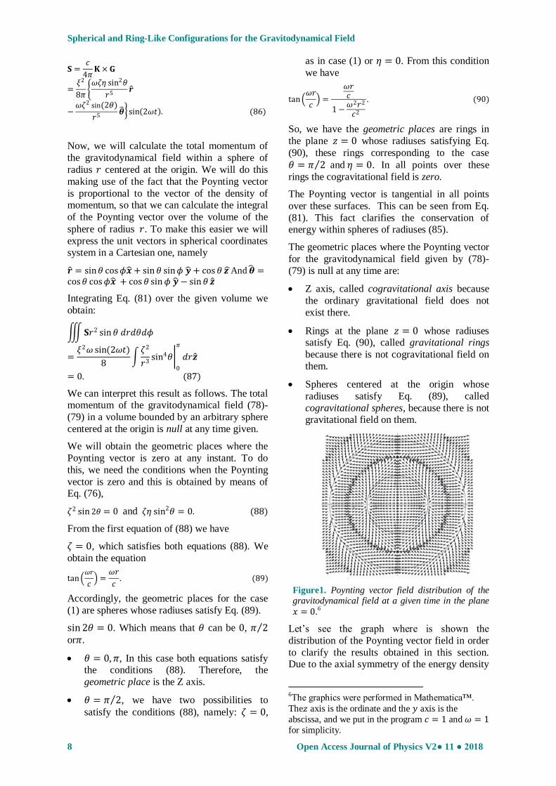
Figure1. Poynting vector field distribution of the gravitodynamical field at a given time in the plane

𝑥 = 0.6

Let’s see the graph where is shown the

distribution of the Poynting vector field in order

to clarify the results obtained in this section. Due to the axial symmetry of the energy density

6The graphics were performed in Mathematica™.

The𝑧 axis is the ordinate and the 𝑦 axis is the

abscissa, and we put in the program 𝑐 = 1 and 𝜔 = 1

for simplicity.



and the energy-flux density, we can consider

only the distribution in the plane𝑥 = 0.

In Fig. 1 we can see the vertical cogravitational

axis that matches with the 𝑧 axis, And we ca

also see the cross-section of three spheres, which we will call G-sphere to the first one, K-

sphere to the second one, and G-sphere to the

last one7, in an arbitrary instant. The total

gravitodynamical energy conserves within G-spheres due to theenergy-flux vector at the

surface of this sphere has tangential component

only.

We can see also that energy transfers from these

G-spheres to the gravitational ring (the equator

of such spheres) and after a period defined by

the function sin(2𝜔𝑡) in Eq. (81) the movement is reversed. Inside the first G-sphere the energy

transfers from the cogravitational axis to the

gravitational ringand having spent some time returns. The energy within the K-sphere is also

conserved, we can see this because the Poynting

vector is zero in every point of the K-sphere graphed. The energy is transferred from the

surface of the K-sphere to the gravitational rings

of the G-spheres. An analogue exchange of

energy occurs between next G-spheres and K-spheres.

We want to emphasize the fact that the Poynting

vector field reverses their direction after a time

due to the function sin(2𝜔𝑡) present in Eq. (86).

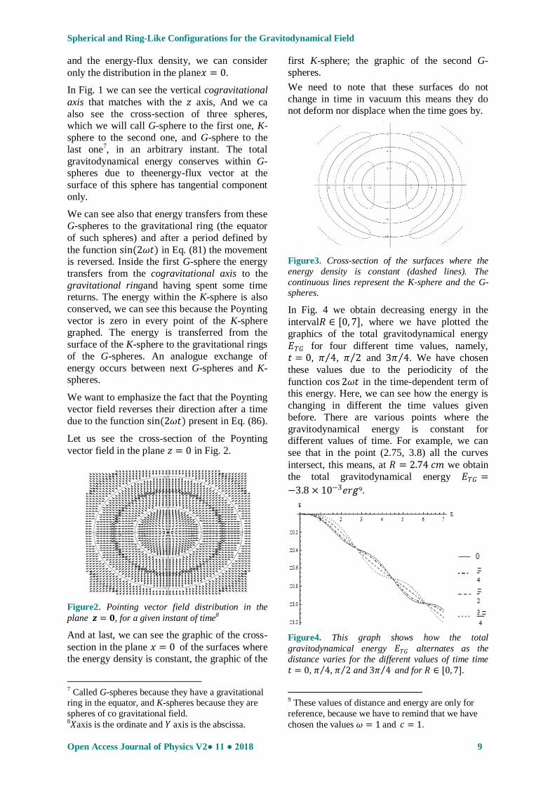
Let us see the cross-section of the Poynting

vector field in the plane 𝑧 = 0 in Fig. 2.

Figure2. Pointing vector field distribution in the

plane 𝒛 = 𝟎, for a given instant of time8

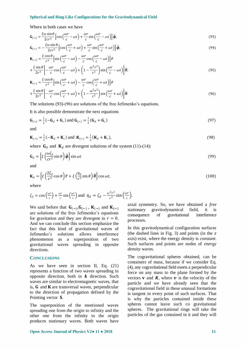
And at last, we can see the graphic of the cross-

section in the plane 𝑥 = 0 of the surfaces where the energy density is constant, the graphic of the

7 Called G-spheres because they have a gravitational ring in the equator, and K-spheres because they are

spheres of co gravitational field. 8𝑋axis is the ordinate and 𝑌 axis is the abscissa.

first K-sphere; the graphic of the second G-

spheres.

We need to note that these surfaces do not

change in time in vacuum this means they do not deform nor displace when the time goes by.

Figure3. Cross-section of the surfaces where the

energy density is constant (dashed lines). The

continuous lines represent the K-sphere and the G-spheres.

In Fig. 4 we obtain decreasing energy in the

interval𝑅 ∈ [0, 7], where we have plotted the

graphics of the total gravitodynamical energy

𝐸𝑇𝐺 for four different time values, namely,

𝑡 = 0, 𝜋 4 , 𝜋 2 and 3𝜋 4 . We have chosen

these values due to the periodicity of the

function cos 2𝜔𝑡 in the time-dependent term of this energy. Here, we can see how the energy is

changing in different the time values given

before. There are various points where the

gravitodynamical energy is constant for different values of time. For example, we can

see that in the point (2.75, 3.8) all the curves

intersect, this means, at 𝑅 = 2.74 𝑐𝑚 we obtain

the total gravitodynamical energy 𝐸𝑇𝐺 =

−3.8 × 10−3𝑒𝑟𝘨9.

Figure4. This graph shows how the total

gravitodynamical energy 𝐸𝑇𝐺 alternates as the

distance varies for the different values of time time

𝑡 = 0, 𝜋 4 , 𝜋 2 and 3𝜋 4 and for 𝑅 ∈ [0, 7].

9 These values of distance and energy are only for

reference, because we have to remind that we have

chosen the values 𝜔 = 1 and 𝑐 = 1.



Now, we want to show both dependences in 3D

graphics, and we are going to analyze them. Due to the periodicity of the term time-dependent we

will fix them for 𝑡 ∈ [0, 2𝜋]. First, we have Fig.

5(a) the interval 𝑅 ∈ [0, 1 ].

Figure5(a). Graph of the total gravitodynamical

energy contained in the G- and K-spheres. 𝐸𝑇𝐺 for

the intervals 𝑅 ∈ [0, 1 ] and 𝑡 ∈ [0, 2𝜋].

In the Fig. 5 (b) we show the total

gravitodynamical energy in the interval𝑅 ∈[0, 10].

Figure5(b).Total gravitodynamical energy in the

interval 𝑅 ∈ [0, 10].

Figure6.Contour plot of the total gravitational

energy in the intervals 𝑅 ∈ [0,1.25]and𝑡 ∈ [0, 2𝜋]. The cross-section where the total gravitodynamical

energy is null, forms semi-ovoid.

At last, we want to show the graphics of the

cross-sections of both fields, in Fig. 7 we have

the gravitational field in the plane 𝑧 = 0. In Fig.

8 we have drawn cross-sections of the

cogravitational field in the planes 𝑦 = 0 and

𝑥 = 0 respectively.

Figure7. Ring-like form of the gravitational field in

the plane 𝑧 = 0.

Figure8.Cogravitational field in the planes 𝑦 = 0

and 𝑥 = 0, this field does not have components in

the plane 𝑧 = 0.

Convergent Solution (78) and (79)

Represented as a Superposition of Two

Divergent Solutions

We can represent solutions (78) and (79) as a

superposition of two waves spreading in

opposite directions in each point, as the same way as Eq. (21). To do that only we need to do

an algebraic transformation.

We call

𝐆𝑐 = 𝐆(→) + 𝐆 ← (91)

Gravitational co nvergent solution. This 𝐆𝑐 is the

superposition of the two waves 𝐆(→) and

𝐆(←)spreading in opposite directions at every

point. In a similar way, we call

𝐊𝑐 = 𝐊(→) + 𝐊 ← (92)

co gravitational convergent solution. These

solutions converge in 𝑟 = 0 ⟺ 𝛿 = (𝑛 +1 2 )𝜋, where, 𝑛 = 0, ±1, ±2, ±3, …



Where in both cases we have

𝐆(→) =𝜉𝜔 sin𝜃

2𝑐𝑟2 cos

𝜔𝑟

𝑐− 𝜔𝑡 +

𝜔𝑟

𝑐sin

𝜔𝑟

𝑐− 𝜔𝑡 𝝓 , (93)

𝐆(←) = −𝜉𝜔 sin 𝜃

2𝑐𝑟2 cos

𝜔𝑟

𝑐+ 𝜔𝑡 +

𝜔𝑟

𝑐sin

𝜔𝑟

𝑐+ 𝜔𝑡 𝝓 , (94)

𝐊(→) =𝜉 cos 𝜃

𝑟3 sin

𝜔𝑟

𝑐− 𝜔𝑡 −

𝜔𝑟

𝑐cos

𝜔𝑟

𝑐− 𝜔𝑡 𝒓

+𝜉 sin 𝜃

2𝑟3 −

𝜔𝑟

𝑐cos

𝜔𝑟

𝑐− 𝜔𝑡 + 1 −

𝜔2𝑟2

𝑐2 sin

𝜔𝑟

𝑐− 𝜔𝑡 𝜽 , (95)

𝐊(←) =𝜉 cos 𝜃

𝑟3 sin

𝜔𝑟

𝑐+ 𝜔𝑡 −

𝜔𝑟

𝑐cos

𝜔𝑟

𝑐+ 𝜔𝑡 𝒓

+𝜉 sin 𝜃

2𝑟3 −

𝜔𝑟

𝑐cos

𝜔𝑟

𝑐+ 𝜔𝑡 + 1 −

𝜔2𝑟2

𝑐2 sin

𝜔𝑟

𝑐+ 𝜔𝑡 𝜽 . (96)

The solutions (93)-(96) are solutions of the free Jefimenko’s equations.

It is also possible demonstrate the next equations

𝐆(→) =1

2 −𝐆𝑑 + 𝐆𝑐 and 𝐆(←) =

1

2 𝐆𝑑 + 𝐆𝑐 (97)

and

𝐊(→) =1

2 −𝐊𝑑 + 𝐊𝑐 and 𝐊(←) =

1

2 𝐊𝑑 + 𝐊𝑐 , (98)

where 𝐆𝑑 and 𝐊𝑑 are divergent solutions of the system (11)-(14):

𝐆𝑑 = 𝜉 𝜔𝜁𝑑

𝑐𝑟2sin 𝜃 𝝓 sin 𝜔𝑡 (99)

and

𝐊𝑑 = 𝜉 2𝜁𝑑


𝜂𝑑

𝑟3sin 𝜃 𝜽 cos 𝜔𝑡, (100)

where

𝜁𝑑 = cos 𝜔𝑟

𝑐 +

𝜔𝑟

𝑐sin

𝜔𝑟

𝑐 and 𝜂𝑑 = 𝜁𝑑 −

𝜔2𝑟2

𝑐2 sin 𝜔𝑟

𝑐 .

We said before that 𝐆(→),𝐆(←) , 𝐊(→) and 𝐊(←)

are solutions of the free Jefimenko’s equations

for gravitation and they are divergent in 𝑟 = 0. And we can conclude this section emphasize the

fact that this kind of gravitational waves of

Jefimenko’s solutions allows interference phenomenon as a superposition of two

gravitational waves spreading in opposite

directions.

CONCLUSIONS

As we have seen in section II, Eq. (21)

represents a function of two waves spreading in

opposite direction, both in 𝒌 direction. Such

waves are similar to electromagnetic waves, that

is, 𝐆 and 𝐊 are transversal waves, perpendicular

to the direction of propagation defined by the

Pointing vector 𝐒.

The superposition of the mentioned waves

spreading one from the origin to infinity and the other one from the infinity to the origin

produces stationary waves. Both waves have

axial symmetry. So, we have obtained a free stationary gravitodynamical field, it is

consequence of gravitational interference

processes.

In this gravitodynamical configuration surfaces

(the dashed lines in Fig. 3) and points (in the 𝑧

axis) exist, where the energy density is constant.

Such surfaces and points are nodes of energy density waves.

The cogravitational spheres obtained, can be

containers of mass, because if we consider Eq. (4), any cogravitational field exerts a perpendicular

force on any mass to the plane formed by the

vectors 𝐯 and 𝑲, where 𝒗 is the velocity of the

particle and we have already seen that the cogravitational field in these unusual formations

is tangent in every point of such surfaces. That

is why the particles contained inside these spheres cannot leave such co gravitational

spheres. The gravitational rings will take the

particles of the gas contained in it and they will



turn them in a direction of rotation of such a

field.

From figure 4 we can see the points where the

energy is constant, such points are those where

the different curves are intersected and they represent the nodes of energy waves.

ACKNOWLEDGEMENTS

We would to like to thanks to CONACyT, especially to the Master Pablo RojoDirector of

National Scholarship Allocation and Gabriela

Gomez Deputy Director of National Scholarship Allocation, for the opportunity given to the

Master in Physical Sciences David A. Perez

Carlos to continue the studies in the doctorate in

physical sciences. And in general, to all people working in CONACyT.

REFERENCES

[1] Heaviside O 1893 A gravitational and

electromagnetic Analogies. The Electrician 31

5125-5134.

[2] Jefimenko O D 2000 Causality, electromagnetic

induction and gravitation: A different approach

to the theory of electromagnetic and gravitational fields(Princeton, NJ: Princeton University

Press)

[3] Jefimenko O D 2006Gravitation and Co

gravitation: Developing Newton's Theory of

Gravitation to its Physical and Mathematical

Conclusion (Waynesburg, PA: Electret

Scientific Star City)

[4] Espinoza A, Chubykalo A and Perez Carlos D

2016Gauge Invariance of Gravitodynamical

Potentials in the Jefimenko’s Generalized

Theory of Gravitation Journal of Modern

Physics 7 1617-1626

[5] Assis A K T 2007Gravitation and Cogravitation

Annales de la Fonda tión Louis de Broglie32

117-120.

[6] González W S 2013 Gravito electromagnetismo y principio de Mach (Cádiz: e WT Ediciones)

[7] Creighton J D and Anderson W

G2012 Gravitational-wave physics and astronomy:

An introduction to theory, experiment and data

analysis(Hoboken, NJ: John Wiley & Sons)

[8] Chubykalo A and Espinoza A2002Unusual

formations of the free electromagnetic field in

vacuum. Journal of Physics A: Mathematical

and General 35 8043-8056

[9] Espinoza A and Chubykalo A2003 Mathematical

Foundation of Kapitsa's Hypothesis about the

Origin and Structure of Ball Lightning Foundations

of Physics 33 863-873

[10] Kapitsa P L 1955On the nature of ball

lightning Dokl. Acad. Nauk SSSR101 245-246

(in Russian)

[11] Einstein A 1916 Relativity: The special and general theory (London: Methuen & Co Ltd)

[12] Logunov AA and Mestvirishvili M A 2001

Relativistic theory of gravitation (Moscow:

Mir publishers)

spherical and ring-like configurations for the ... · introduction the jefimenko’s equations...

Documents