spextool: a spectral extraction package for spex, a 0.8–5...

362

Publications of the Astronomical Society of the Pacific, 116:362–376, 2004 April� 2004. The Astronomical Society of the Pacific. All rights reserved. Printed in U.S.A.

Spextool: A Spectral Extraction Package for SpeX, a 0.8–5.5 MicronCross-Dispersed Spectrograph

Michael C. Cushing,1,2

Institute for Astronomy, University of Hawai‘i, 2680 Woodlawn Drive, Honolulu, HI 96822; [email protected]

William D. Vacca1

NASA Ames Research Center, MS 144-2, Moffett Field, CA 94035; and Department of Astronomy, University of California, 601 Campbell Hall, Berkeley,CA, 94720; [email protected]

andJohn T. Rayner

Institute for Astronomy, University of Hawai‘i, 2680 Woodlawn Drive, Honolulu, HI 96822; [email protected]

Received 2003 May 9; accepted 2004 January 15; published 2004 April 2

ABSTRACT. We describe an IDL-based package for the reduction of spectral data obtained with SpeX, amedium-resolution, 0.8–5.5mm cross-dispersed spectrograph and imager for the NASA Infrared Telescope Facility.The package, called Spextool, carries out all the procedures necessary to produce fully reduced spectra includingpreparation of calibration frames, processing and extraction of spectra from science frames, wavelength calibrationof spectra, and flux calibration of spectra. The package incorporates an “optimal extraction” algorithm for point-source data and also generates realistic error arrays associated with the extracted spectra. Because it is fairlyquick and easy to use, requiring minimal user interaction, Spextool can be run by observers at the telescope toestimate the signal-to-noise ratio of their data. We describe the procedures incorporated into Spextool and showexamples of extracted spectra.

1. INTRODUCTION

Cross-dispersed spectrographs provide one of the most ef-ficient means of acquiring spectroscopic data from celestialsources, because they record a broad wavelength range in asingle exposure. Concomitant with the increase in efficiency,however, is a substantial increase in the complexity of themethods needed to reduce these data. Usually the spectral or-ders are curved and irregularly spaced on the detector so thatthe dispersion axis is not aligned with the detector rows. Inaddition, the spatial axis is sometimes not aligned with thedetector columns, so that a given wavelength may span manycolumns along the slit. These properties can make the extractionand calibration of cross-dispersed spectra particularlychallenging.

Until recently, cross-dispersed spectrographs have beenmainly limited to optical wavelengths. However, with the ad-vances in near-infrared detector technology, a new generation ofcross-dispersed spectrographs sensitive in the 1–5mm range has

1 Visiting Astronomer at the Infrared Telescope Facility, which is operatedby the University of Hawai‘i under contract from the National Aeronauticsand Space Administration.

2 Current address: SETI Institute, NASA Ames Research Center, MS 245�3,Moffett Field, CA 94035.

been developed. One such instrument is SpeX (Rayner et al.2003), a medium-resolution ( ), 0.8–5.5mmR { l/Dl ∼ 2000spectrograph operating at the 3.0 m NASA Infrared TelescopeFacility on Mauna Kea.

In an effort to provide a set of semiautomatic routines forreducing SpeX data, we have developed a spectral extractionand reduction package called Spextool (spectral extractiontool). Written in the interactive data language (IDL), this pack-age is driven by a set of graphical user interfaces (GUIs) inwhich a user specifies various parameters pertinent to the re-duction procedures and performs the reductions with a fewmouse clicks.

In this paper, we present a description of Spextool and pro-vide examples of spectra reduced with Spextool. In § 2 webriefly describe the aspects of SpeX that relate to the datareduction process. In § 3 we describe the typical observingmodes used with SpeX. In § 4 we provide a detaileddescriptionof the reduction procedures carried out by Spextool, and in§ 5 we give a summary.

2. SpeX

A full description of the design, construction, and perfor-mance of SpeX is provided by Rayner et al. (2003). Here we

SPECTRAL EXTRACTION TOOL FOR SPEX 363

2004 PASP,116:362–376

TABLE 1SpeX Observation Modes

ModeWavelength Range

(mm) Ra

Slit Lengths(arcsec)

Short XD . . . . . . . . . . . . . . . . 0.8–2.4 200–2000 15Long XD1.9 . . . . . . . . . . . . . 1.9–4.2 250–2500 15Long XD2.1 . . . . . . . . . . . . . 2.1–5.0 250–2500 15Long XD2.3 . . . . . . . . . . . . . 2.3–5.4 250–2500 15Low Resolution . . . . . . . . . 0.8–2.5 25–250 15, 60Short Single Order. . . . . . 0.8–2.5b 200–2000 15, 60Long Single Order. . . . . . 1.9–5.5b 250–2500 15, 60

a R is the resolving power and is given by ; the two valuesR p l/Dl

correspond to the widest (3�.0) and narrowest (0�.3) slits, respectively.b Requires multiple grating settings to achieve full wavelength coverage.

Fig. 1.—Raw SXD flat-field exposure. The spatial axis is parallel to thecolumns and wavelength increases to the right. The six cross-dispersed orders(3–8; bottom to top) are apparent. The diagonal lines are 1 pixel wide cracksin the array. The spot at the approximate coordinates (600, 275) is a clustersof bad pixels. The faint interorder flux is due to scattered light and internalreflections (“ghosts”) and is typically at a level of∼1% of the signal in thebrightest order.

will discuss only those aspects of the instrument that are rel-evant to the data reduction process.

Table 1 provides a summary of the various observing modesfor SpeX. Spextool was designed primarily to extract spectrafrom the cross-dispersed modes, since single-order spectra canbe extracted easily using other data reduction packages (e.g.,IRAF). The short-wavelength cross-dispersed (SXD) mode ofSpeX covers the wavelength range 0.8–2.4mm with an averageresolving power for a slit width of 0�.3. The entireARS p 2000wavelength range, except for a 0.6mm gap in the telluric bandbetween theH and K bands, is recorded simultaneously in 6orders. As can be seen in Figure 1, the spectral orders aresubstantially curved, and the spacing between the orders varieswith position on the array. The long-wavelength cross-dis-persed (LXD) mode covers the wavelength range 1.9–5.5mmwith for a slit width of 0�.3. The entire wavelengthARS p 2500range, except for a 0.1mm gap centered at 4.4mm, is coveredin 7 orders, but only 6 orders can be recorded simultaneouslyon the detector. Therefore, the LXD mode actually consists ofthree submodes (LXD1.9, LXD2.1, and LXD2.3) that coverslightly different wavelength ranges (see Table 1). Both cross-dispersed modes have a slit length of 15�, which correspondsto ∼100 pixels on the detector. Spextool also has the ability toreduce data taken in the LOWRES (prism) mode with the 15�long slit (∼100 pixels); this mode covers the wavelength range∼0.8–2.5mm at for a slit width of 0�.3. Wider slitsARS p 250(0�.5, 0�.8, 1�.6, and 3�.0) are also available for each mode andprovide proportionally lower resolving powers. The pixel sizefor all three modes is 0�.15 pixel�1, so even during the bestseeing conditions currently attainable at the IRTF (∼0�.4 at 2.2mm), the point-spread function is sampled by∼3 pixels. As aresult, intrapixel sensitivity variations (e.g., Lauer 1999) arenot a concern for the data reduction process.

The gratings are operated in the near-Littrow configuration,which means, in principle, the image of the slit should not betilted with respect to the detector columns (Schroeder 2000).In practice, however, the image of the slit is tilted by up to�0.5 pixels over the length of the 15� slit because of predis-persion from the cross-dispersing prisms, the natural curvature

due to any finite-length slit, and the precision to which the slitscan be aligned with the detector columns (see Rayner et al.2003). Since this misalignment is significantly smaller than themaximum spectral resolution delivered by SpeX, we have cho-sen not to attempt to correct for it in Spextool. This greatlysimplifies the data reduction process, since the spectral data donot have to be rectified before extraction.

An external calibration unit contains lamps needed for flat-fielding and wavelength calibration. The flat-field lamps are a10 W quartz-tungsten-halogen lamp (3200 K) and 0.1 W bulbfor the 0.8–2.5mm wavelength range, and an infrared source(1100 K) for the 2.5–5.5mm wavelength range. The unit alsocontains a low-pressure argon discharge lamp for wavelengthcalibration. The lamps are located at the entrance ports of anintegrating sphere. Light from the exit port of the integratingsphere is projected into the spectrograph at the same focal ratioas light from the telescope.

3. OBSERVING TECHNIQUE

It is instructive to discuss the typical manner in which ob-servations are acquired with SpeX, as the observing proceduresdictate, in part, the data reduction process. The number ofcounts recorded in any given detector pixel is given by the sumof the counts from the dark current, emission from the telescopeand sky, and the target. This is an ideal case that ignores anysystematic effects such as array persistence (see Vacca, Cush-ing, & Rayner 2004). In order to remove the dark current,telescope signal, and sky signal (to first order) from the data,observations are usually taken in pairs: anA frame exposureon the target immediately followed by aB frame exposure of

364 CUSHING, VACCA, & RAYNER

2004 PASP,116:362–376

equal integration time to measure the dark current and thetelescope and sky background alone (e.g., Joyce 1992). (Here-after we use a bold letterX to represent an image, and thesubscripted designation to represent the value of the imageX i, j

at the pixel in columni and rowj.) Mathematically we have

A p dark � telescope � sky � target, (1)A

B p dark � telescope � sky , (2)B

where we have explicitly allowed for the possibility that theflux level from the sky may change between theA and Bexposures (e.g., due to the time-variable OH� line emissionfrom 0.8–2.5mm or thermal background from the sky from2.5–5.5mm) but have assumed that the non–sky backgroundsignals, including the dark current and telescope emission, donot (see, however, Rayner et al. 2003). Subtracting theB framefrom theA frame (pair subtraction) gives

A � B p target � sky � sky (3)A B

p target � R, (4)

where we have definedR p skyA � skyB to be the residualsky signal. As long as the signal from the sky in the individualraw A andB frames has not reached the saturation level of thedetector, any residual sky signal can easily be subtracted in theextraction process (see § 4.2.5).

If the object is an extended source, then theB frame is takenafter offsetting (“nodding”) the telescope to a patch of nearbyblank sky so that the object is no longer on the slit (A-skymode). If the object is a point source, however, a more efficientobserving method involves nodding the telescope so that theobject is moved to a new (second) position along the slit andthen taking theB frame exposure (AB mode). In this mode,subtracting theB frame from theA frame leaves both a positiveand negative signal (spectrum) from the object and any residualsignal from the sky. In either mode, the strength of the residualsky signal depends on the variability of the sky and the rapiditywith which the nodding was performed.

In order to correct for absorption from the Earth’s atmo-sphere, as well as to assign physical flux units to the detectedcounts in the extracted object spectrum, observations of a so-called telluric standard star must also be obtained. In additionto the science and telluric standard data, calibration frames thatinclude a series of flat-field exposures as well as argon arcexposures for wavelength calibration are also taken. The objectand standard star exposures, along with the flats and arcs, makeup a single data set.

4. SPECTRAL REDUCTION

The reduction process consists of three main steps:

1. Preparation of calibration frames.—Combine and nor-

malize flat-field exposures and create an arc image suitable forwavelength calibration.

2. Spectral extraction.—Extract and wavelength calibratetarget and standard star spectra.

3.Post-extraction processing.—Correct target spectra for tel-luric absorption, merge spectra from different orders, clean andsmooth spectra, and merge spectra from different modes (SXDand LXD).

A flowchart showing the order of the various steps is shownin Figure 2, and we describe each step in detail in §§ 4.1, 4.2,and 4.3, respectively. The GUI used to perform steps 1 and 2is shown in Figure 3.

4.1. Step 1: Calibration Frames

4.1.1. Flat Fields

As described in § 3, multiple flat-field exposures are takenas part of the calibration set and then combined to maximizethe signal-to-noise ratio (S/N). Before the individual flat-fieldframes are combined, Spextool computes the median signallevel of each frame. It then scales each frame to a commonmedian flux level (the median of the individual median signallevels) to compensate for any variations in the flux levels dueto changes in the temperature of the lamp filaments. Thesetemperature changes also affect the slope of the spectrum pro-duced by the filaments. However, we have found that correctingfor these changes makes almost no difference (less than 0.1%)in the final normalized flat field, and so in the interest of com-putational speed, we do not correct for these changes. Thescaled flat-field exposures are then combined using the statisticchosen by the user (median, mean, or weighted mean).

One of the most important steps in the entire reduction pro-cess is the determination of the location of the orders on thearray. The combined flat-field image, with its high S/N acrossthe entire wavelength range for all the orders, is ideal for thispurpose. Spextool determines the spectroscopy mode in whichthe data were taken by reading the FITS header of the dataframes and retrieves the approximate center positions of eachorder from a file stored on disk. Starting from these centerpositions, an edge detection algorithm moves across the arrayat regularly spaced intervals and locates the bottom and topedge of each order. The individual edge points are then fittedwith a low-order robust polynomial (see Fig. 4,left). The re-sultingedge coefficients then provide the location of each orderat any column. As can be seen in Figure 4 (left), some ordersare truncated by the edges of the array. Therefore, in additionto the edge coefficients, the columns at which the truncationoccurs are also are identified. Spectral extraction proceeds onlybetween the truncation limits, because knowledge of the orderlocation is crucial for the extraction process.

The 15� slit is re-imaged across∼100 pixels, which yieldsan average plate scale of 0�.15 pixel�1. However, because ofanamorphic magnification, the slit height measured in pixels


2004 PASP,116:362–376

Fig. 2.—Flowchart showing the steps in the reduction process used by Spextool.

varies within an order (�3 pixels) and from order to order. Forexample, order 3 in the SXD mode has an average slit heightof 97 pixels, while order 8 has an average slit height of 106pixels. To simplify spectral extraction, all operations that in-volve the spatial dimension are carried out in units of arcse-conds instead of pixels. The arcsecond value of each pixel alongthe slit at a given column is determined by assuming that thelength of the slit in pixels is always equal to 15�.

The flat-field frame must be normalized to unity for usersto obtain estimates of the S/N of their spectra. To facilitate thenormalization process, each order is “straightened” by resam-pling it onto a uniform grid ofi columns ands spatial points.

Since we assume that the reimaged slit is aligned with thecolumns of the array, the resampling proceeds on a column-by-column basis. The result is a rectangular image of the orderuniformly sampled in the spatial dimension. Because the lampsdo not illuminate the slit the same way as the sky does, a two-dimensional surface is then fitted to the straightened order im-age of the flat. The raw flat field is normalized by resamplingthe surface fit back onto the arcsecond grid of the raw datacolumn by column and dividing the result into the raw data.It should be noted that the final normalized flat field has notbeen resampled. The resampling occurs only to construct thesmooth, two-dimensional surface fit. The normalized flat field


2004 PASP,116:362–376

Fig. 3.—Main Spextool GUI.

is then written to disk with the edge coefficients and the trun-cations limits contained in the FITS header. Figure 4 (right)shows an example of a normalized SXD flat field.

4.1.2. Arcs

Wavelength calibration of SpeX data is accomplished usingargon lines. For the SXD and LOWRES modes, several arcexposures are combined to increase the S/N. For the LXDmodes, an “arc off” frame (taken immediately after the arclamp is turned off) is subtracted from an “arc on” frame (takenwith the arc lamp turned on) in order to remove the strongthermal continuum from the heated arc lamp.

For mm the number and strength of the argon linesl � 3

diminish rapidly, and for mm there are no suitablyl 1 4.5strong argon lines that can be used for wavelength calibration.Therefore, to calibrate the LXD modes, we have adopted anapproach that makes use of both the argon lines at shorterwavelengths and the numerous sky emission lines at longerwavelengths. A pure sky frame (for A-sky mode) or two targetframes (for AB mode) are used to produce a night-sky emissionimage. If the object is observed in the AB mode, then this isdone by combining the frames according to the equation

F Fsky p (A � B) � (A � B) . (5)

For those LXD orders (4 and 6) where the arc lines are either


2004 PASP,116:362–376

Fig. 4.—Left: Detection of the edges of the orders in the flat-field image. The red asterisks represent initial guesses for the centers of each order. The greencrosses mark the positions where the order edge is located, and the red lines are the robust polynomial fits through these positions. The blue crosses designatepositions that have been excluded from the fits.Right: A normalized flat field. Note the tree-ring-like structure caused by mechanical thinning of the InSb arraymaterial from 200 to 20mm, and the odd-even eight column pattern due to the eight separate readout locations in the silicon multiplexer. Also visible is a slightdifference in gain between the top half and bottom half of the array, which are read out by two different analog-to-digital converter boards. The spot at theapproximate coordinates (900, 400) is a clusters of bad pixels.

Fig. 5.—LXD2.3 wavelength calibration frame. The five orders (4–8;bottomto top) are apparent. Orders 4 and 6 have been replaced by a sky emissionspectrum.

weak or absent, the sky emission image replaces the arc image.The final image is then written to disk. Figure 5 shows an arcimage for LXD2.3 mode.

4.2. Step 2: Spectral Extraction

4.2.1. Image Processing

The first step in processing the science images involves cor-recting each pixel value in the raw data frames for possiblenonlinearity. Spextool accomplishes this using a nonlinearitycurve constructed by P. Onaka and J. Leong from flat-fielddata taken expressly for this purpose. A series of flats wastaken with gradually increasing exposure times, and the non-linearity curve was then determined by fitting a third-orderpolynomial to the observed count rate as a function of theobserved counts in each pixel. The deviation of this curve froma constant value then gives the factor needed to correct theobserved counts in a given pixel to the expected counts for alinear response.

Unfortunately, as noted by Vacca et al. (2004), the linearitycorrection factor cannot be applied directly to the stored pixelvalues, because the array is read out using multiple correlateddouble sampling (MCDS; Fowler & Gatley 1990), also knownas Fowler sampling. In this readout mode, the array is read outnondestructively times at the start of the integration. Afternr

a time (the integration time), the array is again read outDt


2004 PASP,116:362–376

Fig. 6.—Pair-subtracted, flat-fielded SXD frame. The source spectra in eachorder are the strong positive and negative curved lines. Note the regions ofzero source flux due to strong atmospheric absorption. The faint horizontallines seen at columns above 900 in rows 300 and 350 areK-band “ghosts”due to internal reflections in SpeX.

nondestructively times. Each nondestructive read requires anr

time of . Thenet signal, given by the difference between thedtsums of the values recorded for the two sets of nondestructivereads, is then written to disk as an image. If the user requests

“co-adds,” then the readout process is repeated times, andn nc c

the individual net signals are summed in memory and the totalnet signal is written to disk. The linearity correction shouldStot

be applied to the values of the individual nondestructive reads,but only the total net signal is written to disk as an image.Therefore, Spextool determines the nonlinearity correction foreach pixel in each input frame using the iterative techniquedescribed by Vacca et al. (2004).

The linearity-corrected data are then converted to a “flux”cStot

(DN s�1) given byI

cStotI p . (6)n n Dtr c

Because optimal extraction (see § 4.2.5) requires an error es-timate for each pixel in the extraction aperture, Spextool alsoconstructs a variance image for each input image, given byVI

c 2 2S 1 dt (n � 1) 2jtot r readV p 1 � � (7)I [ ]2 2 2 2gn n Dt 3 Dt n g n n Dtr c r r c

whereg is the gain (e� DN�1) and is the rms read noisejread

( ). A derivation of equation (7) is given by Vacca et al.�e(2004).

The next step consists of subtracting an and frame toI IA B

remove the additive components of the recorded signal as de-scribed in § 3. The resulting image is then flat-fielded usingthe normalized flat field created in § 4.1.1. This yields the finalreduced image

I � IA BD p . (8)f lat

The variance image of is given by,D

V � VA BV p . (9)D 2f lat

A pair-subtracted, flat-fielded image of a point source in theSXD mode is shown in Figure 6. Note the positive and negativespectra produced by the pair subtraction.

4.2.2. Spatial Profiles

The spatial profile image gives the relative intensity ofPi, j

a target spectrum at each spatial positionj along the slit at eachcolumn (wavelength)i. The spatial profile varies as a functionof both wavelength (column) and spatial position (row) becauseof small optical effects, atmospheric differential refraction, andwavelength-dependent seeing, which cause changes in the rel-

ative shape and position of the spatial profile (Horne 1986).Constructing an accurate, high-S/N spatial profile image is cru-cial for the optimal extraction procedure. In addition, the meanspatial profile along the slit (averaged over all columnsi) isneeded by the user to define the extraction parameters (see §4.2.4). The procedure used by Spextool to construct the spatialprofile images is a variation on the “virtual resampling” al-gorithm of Mukai (1990).

The spatial profile image for each order is constructed asfollows. If the target is a point source, then the median signallevel in each column (within an order) is subtracted from eachpixel in the column to remove any residual sky background.If the target is an extended source, then no attempt is made tosubtract any residual sky signal, because the sky signal cannotbe measured if the target subtends an angle greater than 15�,the length of the slit. The order is then resampled onto a uniformrectangular grid ofi columns ands spatial points, as describedin § 4.1.1. Figure 7 (top left) shows the resampled image oforder 6 in the SXD mode.

The resampled image of an order can be thought of as aspatial profile image with an intensity modulated by the ob-served spectrum of the object at each wavelength. Therefore,at any given columni and spatial points in the order image,the intensity is given by

O p f P , (10)i, s i i, s

where is the intensity of the source spectrum at column (wave-fi


2004 PASP,116:362–376

Fig. 7.—Top left: Resampled image of order 6 of the SXD mode. Note the positive and negative spectrum produced by the pair subtraction in the AB mode.The sharp peaks are bad pixels.Top right: First-order approximation of the spatial profile image.Bottom left: Model of the spatial profile image created byevaluating the profile coefficients.Bottom right: Average spatial profile.

length) i. If is known, then can be generated easily byf Pi i, s

simple division. (Of course is exactly what we are trying tofi

determine from the observations and so is never known apriori!) The variation in intensity with column can be removedby normalizing each column in by an appropriate scaleOi, s

factor. For optical spectroscopy, the scale factor is given bythe total intensity in a column, which can be calculated bysimply summing the values of the pixel along the column.Dividing each pixel in a column by the total flux in that columnremoves the variation in wavelength, and yields (HornePi, s

1986). However, in the near-infrared, the AB mode of observingproduces both positive and negative images of the spectrum inany column when the two exposures are subtracted, and as aresult, for all i. Therefore, Spextool computes the� f ≈ 0i, ss

profile image in the following iterative manner.First, at each spatial (slit) points, Spextool computes the

median of the columns of the observed order image. This yieldsa one-dimensional array (of lengths) that is the first-orderapproximation to the mean spatial profile . Assuming thatPs

O ≈ c P , (11)i, s i s

Spextool then uses a linear least-squares routine to fit the first-order approximation of to the intensity variation in eachPs

column in the resampled order image and determines the scalefactors . These scale factors are actually the first-order ap-ci

proximations to . The resampled image is then divided by thefi

scale factors, which then yields an approximation to . ThePi, s

result of this procedure, applied to order 6, is shown in Figure7 (top right). The entire procedure can be repeated to yieldbetter approximations to . However, we have found that thisPi, s


2004 PASP,116:362–376

first image is quite satisfactory for optimal extraction pur-Pi, s

poses. Further iterations produce only marginal improvements.Once the spatial profile image is determined, SpextoolPi, s

fits a low-order polynomial along the columnsi at each spatialpoints in the image. This has the effect of smoothing the profileimage, thus increasing its S/N. Columns for which the scalefactors indicate there is no significant source flux are ex-ci

cluded from the polynomial fit. Theprofile coefficients resultingfrom the polynomial fits can be used to determine the valueof the intensity profile at any column and any spatial point.Pi, s

The spatial profile image for order 6, created by evaluating theprofile coefficients, is shown in Figure 7 (bottom left). Theaverage spatial profile , computed from the model spatialPs

profile image, is shown in Figure 7 (bottom right). Finally,is constructed by resampling onto the pixel gridP P (i, j)i, j i, s

using the arcsecond values associated with each pixel.

4.2.3. Aperture Location and Tracing

Once the profile coefficients have been determined, the userspecifies the position of the extraction apertures along the slitusing the average spatial profiles as a guide. If the target is apoint source, Spextool automatically determines the aperture po-sitions by iteratively identifying local maxima in the absolutevalue of the average spatial profiles. If the target is an extendedsource, the user types the locations of the aperture positions,measured in arcseconds from the bottom of the slit (see Fig. 8),into a text field.

Since the location of the extraction apertures are identifiedusing the average spatial profiles, they do not represent the trueposition of the spectrum on the detector at any given column.As discussed in § 4.2.2, this is a result of small optical effectsas well as atmospheric differential refraction. For point sources,this true position is found by tracing the spectra across thearray. A tracing routine steps across the array at regularlyspaced intervals and locates the center of a spectrum by fittinga Gaussian in the spatial dimension centered on the apertureposition defined above. The individual center points are thenfitted as a function of column number with a low-order robustpolynomial. The resultingtrace coefficients provide the locationof that spectrum at any column. This process is repeated foreach aperture and for each order.

Unfortunately, extended sources cannot, in general, betraced, since there is no guarantee that the extraction apertureswill be located at the positions of local maxima in the averagespatial profiles. Therefore, Spextool simply adopts trace co-efficients based on the edge coefficients. Spextool first convertsthe user-specified aperture position (in arcseconds) to a pixelposition at each column using the edge coefficients. The ap-erture positions (in pixels) are then fitted as a function of col-umn number with a low-order robust polynomial to producethe trace coefficients. Therefore, due primarily to atmosphericdifferential refraction, the position of the extraction apertureon the target will vary with wavelength. For most air masses,

this effect can be mitigated by choosing a large enough ex-traction aperture.

4.2.4. Extraction Parameters

The extraction parameters (i.e., extraction apertures andbackground regions) are defined by the user with the aid ofthe average spatial profiles constructed in § 4.2.2. Figure 8shows the average spatial profiles for a point source and anextended source (Uranus) in order 6 of the SXD mode.

For point sources, the parameters are defined with respect toeach aperture position (vertical cyan solid line). The followingextraction parameters are indicated in color in Figure 8:

PSF radius.—The radius in arcseconds at which the PSFprofile falls to zero (blue dotted lines). This parameter is usedonly for optimal extraction (see § 4.2.5).

Aperture radius.—The radius in arcseconds defining theedge of the extraction aperture (green solid and vertical dottedlines).

Background start.—The radius in arcseconds at which tostart the background region.

Background width.—The width in arcseconds of the back-ground region (the background region is shown with a red solidline).

Background fit degree.—The degree of the robust least-squares polynomial fit to the background regions (the fit to thebackground is shown with a magenta dotted line).

For extended sources, the relevant parameters are:

Aperture radii.—The extraction radius for each aperture(green solid and dotted line).

Background regions.—The regions used to fit the back-ground level (red solid lines).

Background fit degree.—The degree of the robust least-squares polynomial fit to the background regions (magentadotted line).

4.2.5. Extracting the Spectra

The spectra can be extracted once the trace coefficients aredetermined and the extraction parameters have been definedby the user. For a given aperture and order, the trace coefficientsare used to determine the position of the spectrum at a givencolumn. The extraction parameters, defined in arcseconds, arethen converted to units of pixels using the edge coefficients.Before the spectra can be extracted, any residual sky signalleft over from the initial pair subtraction (see § 3) must besubtracted from the reduced image (eq. [8]). At each columnDi, the values of the pixels in the user-defined backgroundregions (red solid lines in Fig. 8) are fitted with a low-orderweighted polynomial as a function of their position along theslit. The resulting fit provides an estimate of the residual skylevel at each pixel along the slit in columni. As long asR̃i, j

the raw pixel values in the individual raw and frames areA B


2004 PASP,116:362–376

Fig. 8.—Two examples of the average spatial profiles for order 6 of the SXD mode. The upper profile results from a point source observed in the AB mode;the bottom is an extended source (Uranus) observed in the A-sky mode. The solid vertical cyan lines denote the location of the two apertures. Spextool automaticallyidentified the positions of the two apertures in the upper panel, while we manually selected two apertures located at 6�.3 and 9�.5 in the lower panel. The solidand dotted green lines denote the extraction aperture, while the red lines denote the regions used for the background determination. The magenta dotted linerepresents the polynomial fit to the background regions. The dotted blue lines in the point-source profile represent the PSF radius. The PSF radius is used onlyfor optimal extraction and is therefore not present in the extended source profile.

not saturated, subtracting from removes the residualR̃ Di, j i, j

sky signal.Spextool can extract the spectra from the sky-subtracted

frame ( ) in two ways:sum andoptimal. In the sum˜D � Ri, j i, j

mode, cosmic-ray hits are first identified using the spatial pro-files created in § 4.2.2. At each columni, the spatial profile

is scaled to the data in a robust linear least-squares sense.Pi, j

Any pixels identified as outliers, as well as bad pixels identifiedfrom the bad pixel mask stored on disk, are replaced with thevalue of the scaled profile. The flux and variance of the objectat columni is then given by

j2sum ˜f p e (D � R ),�i i, j i, j i, j

jpj1

j22V p e (V � V ), (12)sum ˜�f i, j D Ri i, j i, j

jpj1

where and are the pixel indices of the upper and lowerj j1 2

limits of the extraction aperture, and is the fractional weightei, j

of pixel ( ), which is given by the fraction the each pixeli, j

contained within the extraction aperture. The value of isei, j

everywhere unity except for the pixels at the edges of theapertures.

Optimal extraction was originally developed by Robertson(1986) and Horne (1986) to maximize the S/N of long-slitspectra of point sources. The method was later expanded byMarsh (1989) and Mukai (1990) to include the extraction ofcross-dispersed spectra, and Naylor (1998) has developed an“optimal extraction” algorithm for point-source photometry.All optimal extraction algorithms work on the same principle,namely, weighting each pixel in the extraction aperture in pro-portion to the amount of flux it contains from the target.

For each aperture, Spextool normalizes using the PSFPi, j

radius defined in § 4.2.4 so that

Pi, jP p , (13)i, j j2� Pi, jjpj1

where and are the upper and lower limits given by thej j1 2

PSF radius. Here now gives the fraction of the total fluxPi, j

from the object contained in pixelj of columni. At each column


2004 PASP,116:362–376

i, then represents an array ofj independent˜(D � R )/Pi, j i, j i, j

estimates of the total flux of the object. These independentestimates are combined in an optimal way using a weightedmean where the weights are given by their inverse variances,

. The flux and variance of the object at column2P /(V � V )˜i, j D Ri, j i, j

i then become

j2 ˜� M P (D � R )/(V � V )˜i, j i, j i, j i, j D Rj i, j i, j1optf p ,i j2 2� M P /(V � V )˜i, j i, j D Rj i, j i, j1

1V p , (14)optf ji 2 2� M P /(V � V )˜i, j i, j D Rj i, j i, j1

where and are the upper and lower limits given by thej j1 2

aperture radius, and is an optional mask to remove badM i, j

pixels.As explained by Horne (1986), optimal extraction provides

an increase in the S/N only for background-limited spectros-copy. Since the SXD mode is source limited for all but thefaintest targets, optimal extraction provides relatively little in-crease in the S/N of the spectra. However, the LXD mode isalmost always background limited because of the strong ther-mal flux of the sky and telescope, and as a result, optimalextraction provides an increase in the S/N of the spectra of upto 25%. Independent of S/N concerns, optimal extraction issuperior to sum extraction because it ignores bad pixels insteadof trying to fix them.

4.2.6. Wavelength Calibration

The spectra are wavelength calibrated using the arc framecreated in § 4.1.2. As discussed there, we use argon lines andsky emission features for wavelength calibration. We have com-piled a list of argon lines from Rao, Humphreys, & Rank (1966)and have removed lines that are blended at , theR p 2500maximum resolving power available with SpeX. We deter-mined the wavelengths of the sky emission features using amodel of the atmospheric transmission computed with ATRAN(Lord 1992). All wavelengths are given in vacuum.

Spextool begins the wavelength-calibration process by ex-tracting arc spectra for each extraction aperture. Argon linesor sky features that are blended at the resolving power of theobject spectra are then pruned from the line list. The approx-imate position of each line in the pruned line list is determinedfrom a previously determined wavelength solution stored ondisk. Due to the combined effects of the nonrepeatability ofthe slit wheel mechanism, flexure in the instrument, and internalmovements due to the thermal recycling of SpeX, the zeropoint of this solution can vary by up to a few pixels. Spextool,therefore, performs a cross-correlation between the arc spec-trum extracted above and an arc spectrum stored on disk (usedto create the solution stored on disk) to determine the zeropoint. The position of each line is then determined by fitting

a Gaussian to a small section of the arc spectrum centered onthe approximate position of each line.

Spextool then determines a single wavelength solution foreach extraction aperture using a variation of the technique out-lined by Hall et al. (1994). This method has two advantagesover determining a wavelength solution on an order-by-orderbasis. First, the overall fit is of higher quality, because all ofthe lines on the array are used in the fit. Second, orders witha small number of lines can still be accurately calibrated. Themethod makes use of the fact that for a fixed groove spacing,the ratio of two wavelengths and , diffracted at the samel l1 2

angle but located in two different orders and , is givenm m1 2

by

l m1 2p . (15)l m2 1

Since we assume the spatial dimension is aligned with the col-umns of the detector (see § 2), a given column corresponds tothe same diffraction angle for all of the orders. Therefore, Spex-tool scales the wavelengths of the identified lines to their equiv-alent wavelengths in a given order using equation (15).′ ′l mFor example, in the SXD mode, a line with mm inl p 2.2order 3 will have mm for .′ ′l p 1.1 m p 6

In principle, a wavelength solution can be computed by fit-ting the scaled lines ( ) as a function of column number and′l

then applying the solution to the individual orders using equa-tion (15). However, we find that such a fit leaves large-scaletrends with order number in the residuals (due to small opticaleffects). To remove these trends, we fit the scaled wavelengthswith a robust two-dimensional polynomial where is a func-′l

tion of both the column numberi and the order numberm:

N Nk l

′ k ll (i, m) p C i m . (16)�� klkp0 lp0

A third-order polynomial in bothi and m ( ) re-N p N p 3k l

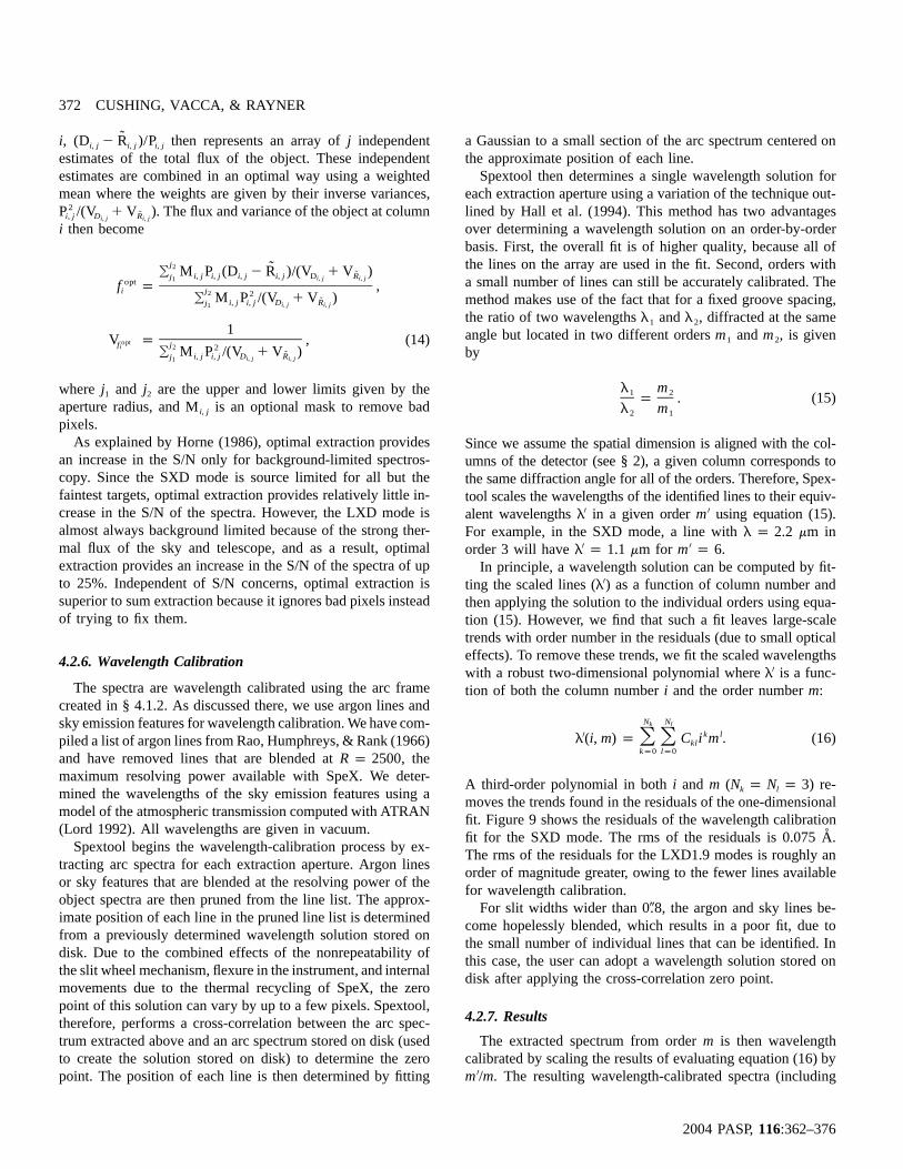
moves the trends found in the residuals of the one-dimensionalfit. Figure 9 shows the residuals of the wavelength calibrationfit for the SXD mode. The rms of the residuals is 0.075 A˚ .The rms of the residuals for the LXD1.9 modes is roughly anorder of magnitude greater, owing to the fewer lines availablefor wavelength calibration.

For slit widths wider than 0�.8, the argon and sky lines be-come hopelessly blended, which results in a poor fit, due tothe small number of individual lines that can be identified. Inthis case, the user can adopt a wavelength solution stored ondisk after applying the cross-correlation zero point.

4.2.7. Results

The extracted spectrum from orderm is then wavelengthcalibrated by scaling the results of evaluating equation (16) by

. The resulting wavelength-calibrated spectra (including′m /m


2004 PASP,116:362–376

Fig. 9.—Residuals of the wavelength-calibration procedure for the SXD mode, shown as a function of spectral order (top) and column (bottom). The rms of theresiduals is 0.075 A˚ .

the error spectra) are written to disk as a FITS file. All of thepertinent extraction parameters are written to the FITS header.Figure 10 shows the SXD and LXD2.1 spectra of the B5 sub-giant HD 147394.

4.3. Step 3: Post-Extraction Processing

4.3.1. Combining the Spectra

For each input image, Spextool produces an output file con-taining the wavelength-calibrated flux and error spectra cor-responding to each extraction aperture in each order. Multipleoutput files (resulting from repeated observations) can be com-bined with a routine that allows the user to choose the com-bining procedure (mean, weighted mean, or median). The spec-tra are resampled onto a common wavelength grid and thencombined.

4.3.2. Telluric Correction

In contrast to the relatively weak telluric absorption featurespresent in the optical, strong absorption bands due to H2O,CO2, and CH4, and to a lesser extent N2O, O2, and O3, dominatethe 1–5mm wavelength range. Therefore, removing the telluricabsorption features in the spectrum of the target is both a nec-essary and critical step in the reduction of infrared spectra.

We have developed a new method for correcting medium-resolution, near-infrared spectra that makes use of an A0 Vstar, observed near in time and close in air mass to the target,and a high-resolution model of Vega. This method simulta-neously removes the instrument signature and approximatelyflux calibrates the target spectrum. A full explanation of themethod, as well as examples of the process, is given by Vacca,Cushing, & Rayner (2003).

4.3.3. Merging the Orders

Once the target spectra have been corrected for telluric ab-sorption, the spectra from the various orders can be merged intoa single, continuous spectrum. In principle, the flux levels andslopes of the spectra from two neighboring orders should matchexactly in their common wavelength range. However, we findsignificant differences in both the flux levels and slopes for someobjects when the nonlinearity correction is not incorporated intothe reduction process (§ 4.2.1). For example, the top panel ofFigure 11 shows the mismatch in flux and slope between theuncorrected spectra from orders 6 (green) and 7 (red) of Gl846 (M0.5 V). The nonlinearity correction removes this prob-lem to a large degree, as can be seen in the lower panel ofFigure 11. For most objects the corrected flux levels in the


2004 PASP,116:362–376

Fig. 10.—Left: SXD spectra of HD 147394 (B5 IV) prior to telluric correction. The overall shape of the spectra is due to the instrument throughput. Strong Habsorption lines can seen in orders 6 and 7. The high-frequency structure is due to telluric absorption.Right: LXD2.1 spectra of HD 147394 prior to telluriccorrection. Most of the structure in these spectra is due to telluric absorption.

order overlap regions differ by�2%. To account for this smalloffset before the spectra from two orders are merged, the usercan scale one of the spectra to match the flux level of the other.One spectrum is then resampled onto the wavelength grid ofthe other, and the two spectra are combined using a weightedmean. The process is continued until all of the orders havebeen merged.

4.3.4. Cleaning and Smoothing the Spectrum

Cleaning and smoothing the spectra are cosmetic in natureand are therefore optional. In principle, the extraction processeither ignores or fixes bad pixels. However, occasionally badpixels are missed and corrupt the spectrum. In addition, thedivision by the telluric correction spectrum can produce strong,high-frequency noise deep in the telluric bands, since the fluxvalues in these wavelength ranges can be close to zero. There-fore, the user can either remove sections of the spectrum thatare noisy, or interpolate over single bad pixels.

For faint objects, it is often advantageous to smooth or rebina spectrum to increase its S/N. The user has the option ofsmoothing the spectrum using a Gaussian kernel or a Savitzky-Golay kernel (Press et al. 1992). The advantage of the latteris that it increases the S/N of the spectrum with minimal lossof resolution.

4.3.5. Merge SXD and LXD Spectra

Finally, if the object has been observed in both the SXDand LXD mode, the spectra from the two modes can be com-bined to produce a single, continuous spectrum. In principle,the flux levels of the SXD and LXD spectra should match, butin practice we often find that the absolute flux levels differ.Therefore, before the spectra from the two modes are combined,one spectrum can be scaled to match the flux level of the other.The LXD spectrum is then resampled onto the wavelength gridof the SXD spectrum, and the two spectra are combined usinga weighted mean.


2004 PASP,116:362–376

Fig. 11.—Spectra of Gl 846 (M0.5 V) from orders 6 and 7 of the SXD mode. The spectra in the upper panel were reduced without applying a correction fornonlinearity; the corrections were incorporated into the reductions of the spectra in the bottom panel. Incorporation of the nonlinearity corrections removes, to alarge degree, the mismatch in both the flux levels and slopes of the spectra in the overlap regions. No additional scaling has been applied to these spectra.

Fig. 12.—The 0.8–5.0mm spectrum of HD 147394 (B5 IV). The break inthe spectrum centered at 1.83mm is a result of a gap in the wavelength coverageof the SXD mode. The spectrum from 2.5 to 2.9mm and from 4.2 to 4.5mmhas been removed because the atmosphere is almost completely opaque atthese wavelengths. The hydrogen absorption lines from the Paschen, Brackett,and Pfund series are indicated. Note the excellent agreement in flux betweenthe separate spectral regions.

4.3.6. Results

Figure 12 shows the approximately flux-calibrated 0.8–5.0mm spectrum of HD 147394 (B5 IV). The resolving power ofthe 0.8–2.5mm spectrum is , and the S/N is greaterARS p 2000than 100; for the 2.1–5.0mm spectrum, , and theARS p 2500S/N is ∼70. The break in the spectrum centered at 1.83mm isa result of a gap in the wavelength coverage of the SXD mode(see Rayner et al. 2003). The spectrum from 2.5 to 2.9mm andfrom 4.2 to 4.5mm has been removed because the atmosphereis almost completely opaque at these wavelengths. The Brack-ett, Paschen, and Pfund series have been identified.

5. SUMMARY

We have presented a description of a new IDL package calledSpextool, which has been developed for the reduction of spec-tral data taken with the near-infrared, medium-resolution, cross-dispersed spectrograph SpeX at the IRTF. Spextool allowsrapid reduction (i.e., flat fielding, aperture definition, sky sub-traction, spectral extraction, wavelength calibration, and vari-ous postprocessing steps) of spectral data acquired in the mostcommonly used spectroscopic modes of SpeX. It generatesrealistic estimates of error arrays associated with spectra, andincorporates an “optimal extraction” algorithm for point-source


2004 PASP,116:362–376

data. A user interacts with Spextool via graphical user interfacesthat incorporate a set of buttons and alphanumeric text fieldsthat specify the various parameters needed for the spectral ex-traction procedures.3

3 The most current version of the package (ver. 3.2) can be downloadedfrom the SpeX website, http://irtfweb.ifa.hawaii.edu/Facility/spex. In addition,

We thank Marc Buie, Nick Kaiser, and John Tonry for helpfuldiscussions, and Peter Onaka and Jonathan Leong for theirwork on the nonlinearity curve. M. Cushing acknowledges fi-nancial support from the NASA Infrared Telescope facility. W.Vacca thanks Alan Tokunaga and James Graham for support.

detailed instructions on how to run Spextool are included in the package andcan also be downloaded from the SpeX website.

REFERENCES

Fowler, A. M., & Gatley, I. 1990, ApJ, 353, L33Hall, J. C., Fulton, E. E., Huenemoerder, D. P., Welty, A. D., & Neff,

J. E. 1994, PASP, 106, 315Horne, K. 1986, PASP, 98, 609Joyce, R. R. 1992, in ASP Conf. Ser. 23, Astronomical CCD Ob-

serving and Reduction Techniques, ed. S. B. Howell (San Francisco:ASP), 258

Lauer, T. R. 1999, PASP, 111, 1434Lord, S. D. 1992, A New Software Tool for Computing Earth’s Atmo-

spheric Transmission of Near- and Far-Infrared Radiation (NASATech. Mem. 103957; Washington: NASA)

Marsh, T. R. 1989, PASP, 101, 1032Mukai, K. 1990, PASP, 102, 183Naylor, T. 1998, MNRAS, 296, 339

Press, W. H., Teukolsky, S. A., Vetterling, W. T., & Flannery, B. P.1992, Numerical Recipes in Fortran 77 (New York: CambridgeUniv. Press)

Rao, K. N., Humphreys, C. J., & Rank, D. H. 1966, WavelengthStandards in the Infrared (New York: Academic Press)

Rayner, J. T., Toomey, D. W., Onaka, P. M., Denault, A. J., StahlbergerW. E., Vacca, W. D., Cushing, M. C., & Wang, S. 2003, PASP, 115,362

Robertson, J. G. 1986, PASP, 98, 1220Schroeder, D. J. 2000, Astronomical Optics (San Diego: Academic

Press)Vacca, W. D., Cushing, M. C., & Rayner, J. T. 2003, PASP, 115, 389Vacca, W. D., Cushing, M. C., & Rayner, J. T. 2004, PASP, 116, 352

spextool: a spectral extraction package for spex, a 0.8–5...

Documents