speed limits set low er than engineering...

i

SPEED LIMITS SET LOWER THAN ENGINEERING RECOMMENDATIONS

Task Report: Literature Review

Prepared by:

Eric T. Donnell Associate Professor

Vikash V. Gayah Assistant Professor

Jeffrey P. Gooch

Graduate Research Assistant

Department of Civil and Environmental Engineering Pennsylvania State University

217 Sackett Building University Park, PA 16082

The Thomas D. Larson

Pennsylvania Transportation Institute 201 Transportation Research Building

University Park, PA 16802

Prepared for: Montana Department of Transportation

October 2014

iii

TABLE OF CONTENTS Table of Contents ........................................................................................................................... iii

List of Tables ................................................................................................................................. iv

List of Figures ................................................................................................................................ iv

Introduction ..................................................................................................................................... 1

Speed ............................................................................................................................................... 1

Posted Speed Limits .................................................................................................................... 1

Design Speed .............................................................................................................................. 2

Operating Speeds ........................................................................................................................ 3

Operating Speeds on Rural Two-Lane Highways .................................................................. 4

Operating Speeds on Multi-lane Highways ............................................................................ 8

Role of Posted Speed Limit in Operating Speed Models ..................................................... 10

State Practices for Setting Posted Speed Limits ....................................................................... 10

Conflicting Design Speeds and Speed Limits ........................................................................... 11

National Maximum Speed Limit .......................................................................................... 12

Work Zone Speed Limits ...................................................................................................... 12

Seasonal Speed Limits .......................................................................................................... 14

Speed Limit Transition Zones ............................................................................................... 15

Speed Limit Compliance and Enforcement .................................................................................. 16

Speed Choice and Compliance ................................................................................................. 16

Enforcement .............................................................................................................................. 17

Speed and Safety ........................................................................................................................... 21

Speed and Crash Severity ......................................................................................................... 25

Speed Enforcement and Safety ................................................................................................. 26

Conclusion .................................................................................................................................... 27

References ..................................................................................................................................... 29

iv

LIST OF TABLES Table 1 – V85 Prediction Models for Two-Lane Rural Highways ................................................. 6 Table 2 – Speed Models Developed by Jessen et al. (2001) ........................................................... 7 Table 3 – Summary of Descriptive Statistics for Work Zone Speed Limit Compliance .............. 13 Table 4 – Results of OLS Operating Speed Models in Transition Zones ..................................... 16 Table 5 – Designs of Speed Limit Enforcement Field Studies ..................................................... 17 Table 6 – Summary of Halo Effects ............................................................................................. 20 Table 7 – Power Model Coefficients from Meta-Analysis ........................................................... 23 Table 8 – Summary of Speed Related CMF Studies (FHWA 2014b) .......................................... 24 Table 9 – Odds ratio of injury by severity and study sites versus comparison sites..................... 26

LIST OF FIGURES Figure 1 – Depiction of the relationship between inferred design speed and other speeds ............ 3 Figure 2 – Crash involvement as a function of speed for daytime and nighttime crashes ........... 21 Figure 3 – CMF for relative speed enforcement. .......................................................................... 27

1

INTRODUCTION The Montana Department of Transportation has implemented posted speed limits lower than engineering recommendations on several roadways, and would like to quantify the effects of this practice on vehicle speed and safety. Current research regarding speed and safety performance on roadways with posted speed limits set lower than engineering recommendations is limited. To account for this limitation in the published literature, this review broadly considers the relationship between various speed measures and safety. The literature review begins with a discussion of speed concepts, including the relationship between posted speed limits, operating speeds, and design speeds. Issues related to speed compliance and enforcement are then described. The literature review concludes with a brief discussion of the effects of speed on safety.

SPEED This section of the report focuses on the posted speed limit, design speed, and operating speed. The speed limit is the maximum allowable speed at which a vehicle can legally traverse a roadway. The design speed of a roadway is one of the controlling criteria for a roadway and is used directly and indirectly to establish many characteristics of a highway alignment and cross-section (AASHTO 2011). The operating speed is defined as the speed at which vehicles are observed under free-flow conditions. The most common operating speed measure is the 85th percentile of the speed distribution. Each of these speed concepts is described in more detail below.

POSTED SPEED LIMITS Posted speed limits are conveyed by regulatory signs and are established in increments of five miles per hour (mph). The Federal Highway Administration’s (FHWA) SPEED CONCEPTS: INFORMATION GUIDE (Donnell et al. 2009) describes two methods for establishing posted speed limits: legislative/statutory and an engineering study. A statutory (or legislative) speed limit is established by law and often provides maximum posted speed limits based on specific roadway categories (e.g., local street or urban arterial). This method is often criticized for its arbitrary assignment of speed limits independent of site characteristics. Enforcement officials are challenged to manage operating speeds on roadways with statutory speed limits due to their arbitrary assignment (Transportation Research Board 1998).

An engineering study consists of collecting a sample of free-flow vehicle operating speeds during daylight and compiling a speed distribution. The 85th percentile speed of the sample data is most often used to establish the posted speed limit. Being that this speed limit is based on field data, the posted speed limit is much more reliable in identifying drivers travelling at excessive speeds. This process implies that only a limited proportion of vehicles (15 percent) will violate the posted speed limit. In practice, the number of speed limit violators is likely even fewer because enforcement officers typically provide a 5-10 mph allowance over the posted speed limit before offering traffic citations (Transportation Research Board 1998). Specific instructions for

2

undertaking a spot speed study are laid out by the Institute of Transportation Engineers (ITE) in MANUAL OF TRANSPORTATION ENGINEERING STUDIES (Institute of Transportation Engineers 2010). Posted speed limits based on the results of this study are often considered more rational than posted speed limits based on legislative policy.

The definition of a vehicle operating under “free-flow” conditions varies. Most studies classify a vehicle in free-flow conditions based on a minimum time headway. Hauer, Ahlin, and Bowser (1981) selected 4 seconds as the minimum headway value based on previous research, which indicated that drivers adjust speed at headways of less than 3 seconds (Ahlin 1979). Misaghi and Yassan (2005) considered vehicle headways of less than 5 seconds as non-free-flow. The Highway Capacity Manual procedure requires vehicles to have a leading headway of 8 seconds as well as a lagging (or following) headway of 5 seconds (Transportation Research Board 2010).

Two other, but less common, methods for setting speed limits are optimization and the expert system approach (Forbes et al. 2012). Optimization is an approach in which all “costs” associated with transportation (safety, travel time, fuel consumption, noise, and pollution) are considered and the speed limit is selected to minimize the total sum of these costs. The expert system approach utilizes a computer program with an extensive knowledge base to recommend a speed limit based on prior experience. A current example of the expert system approach is FHWA’s USLIMITS2, a tool for communities that lack access to engineers with experience in establishing speed limits. USLIMITS2 has been used in over 3,000 projects with users from a wide range of backgrounds (federal, state, local government, non-profits, consultants, and even law enforcement) (FHWA 2014a). Examples of specific uses of USLIMITS2 include: verifying the findings of an engineering speed study to increase a speed limit in Michigan; using site characteristics to determine if a speed limit should be reduced in Indiana; and, checking the validity of speed limits during a statewide safety analysis in Wisconsin (Warren, Xu, and Srinivasan 2013).

DESIGN SPEED The American Association of State Highway Transportation Officials’ (AASHTO) A POLICY ON GEOMETRIC DESIGN OF HIGHWAYS AND STREETS (AASHTO 2011), commonly referred to as the AASHTO GREEN BOOK, uses the design speed concept to produce design consistency. Using this concept, a design speed is selected for a roadway and then used as a direct or indirect input to many geometric design criteria, such as horizontal alignment, vertical alignment, sight distance, and cross-section elements.

The equations that provide design criteria based on the design speed are often conservative. This fact, combined with conservative decision-making in the design process, results in roadway environments that often encourage drivers to travel faster than the intended design speed. This results in an “inferred” design speed being communicated to the driver (Donnell et al. 2009) and operating speeds that are sometimes higher than the design speed of the roadway.

This concept was first introduced as “critical design speed”, which was defined as the minimum calculated design speed from each geometric element along a roadway (Poe, Tarris, and Mason Jr. 1996). This idea was studied in more detail in SPEED CONCEPTS: INFORMATION GUIDE,

3

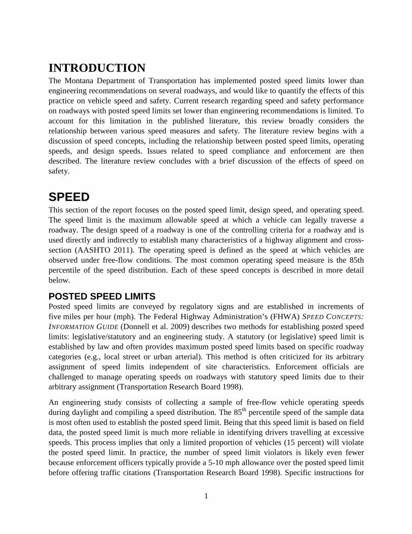
which formally defined the inferred design speed as “the maximum speed for which all critical design speed-related criteria are met at a particular location.” This inferred design speed is determined by calculating the speed using the actual geometry of a specific element. For instance, the inferred design speed of a crest vertical curve is the maximum speed at which minimum stopping sight distance is provided based on the curve’s actual design. The inferred design speed is always greater than or equal to the designated design speed used to design the roadway, whereas the posted speed limit is set equal to or below the designated design speed. An example of the relationship between these different speed definitions is depicted graphically in Figure 1.

FIGURE 1 – DEPICTION OF THE RELATIONSHIP BETWEEN INFERRED DESIGN SPEED AND OTHER SPEEDS

SOURCE: DONNELL ET AL. (2009)

OPERATING SPEEDS Operating speed is the speed that drivers choose to operate their vehicle on a highway. The two most common metrics used to describe operating speeds in the published literature are the mean travel speed and the 85th percentile speed (most common) under free-flow operating conditions. Some engineering studies also describe operating speeds by the 10 mph range in which the highest fraction of drivers is observed, defined as the pace. The pace is particularly useful as it provides the range of speeds that are most commonly expected at a particular location. However, the pace is much less commonly used in practice than the 85th percentile or mean free flow speed.

A significant amount of published literature exists on the development of models to predict operating speeds based on geometric and other roadway characteristics. Much of this research is

4

focused on producing statistical models of vehicle operating speeds to objectively quantify the design consistency of two-lane rural highways (in place of the AASHTO Green Book design speed concept). Dimaiuta et al. (2011) performed an extensive review of speed models in North America, covering both two-lane rural roads and multilane rural highways and freeways. The following sections provide a summary of their findings.

OPERATING SPEEDS ON RURAL TWO-LANE HIGHWAYS Most research on two-lane rural road operating speeds has focused on estimating the 85th percentile speeds of passenger cars on horizontal curves. The majority of studies find that the radius of the horizontal curve is most closely associated with the mean or 85th percentile operating speed (Dimaiuta et al. 2011; McFadden, Yang, and Durrans 2001; McFadden and Elefteriadou 2000; Fitzpatrick et al. 2000; Donnell et al. 2001; Voigt and Krammes 1996; Misaghi and Hassan 2005; Islam and Seneviratne 1994; Krammes et al. 1995). All of the studies covered in Dimaiuta et al. found that the 85th percentile speeds on the curve decreases as the radius of the curve decreases.

Islam and Seneviratne (1994) measured spot speeds at eight horizontal curves in Utah. Degrees of curvature on these curves ranged between 4 and 28 degrees. Speeds were measured at the start (PC), midpoint (MC), and end (PT) of the curve. The following models were developed for each location along the curve:

𝑉85𝑃𝑃 = 95.41 − 1.48𝐷𝐷 − 0.012𝐷𝐷2 𝑅2 = 0.99

𝑉85𝑀𝑃 = 103.30 − 2.41𝐷𝐷 − 0.029𝐷𝐷2 𝑅2 = 0.98

𝑉85𝑃𝑃 = 96.11 − 1.07𝐷𝐷 𝑅2 = 0.98

where

V85PC = predicted 85th percentile speed at PC (km/h)

V85MC = predicted 85th percentile speed at the midpoint of the curve (km/h)

V85PT = predicted 85th percentile speed at PT (km/h)

DC = degree of curvature (degrees per 30 m of arc)

Voigt and Krammes (1996) modeled simple horizontal curve speeds on 138 curves from New York, Pennsylvania, Oregon, Texas, and Washington. Speeds were modeled using degree of curvature, length of curve, superelevation rate, and deflection angle. Linear regression was used to develop the following models:

𝑉85 = 102.0 − 2.08𝐷𝐷 + 40.33𝑒 𝑅2 = 0.81

𝑉85 = 99.6 − 1.69𝐷𝐷 + 0.014𝐿 − 0.13𝐷𝑒𝐷𝐷𝐷 + 71.82𝑒 𝑅2 = 0.84

where

V85 = 85th percentile speed at the midpoint of the curve (km/h)

5

e = superelevation rate (m/m)

L = length of curve (m)

Delta = deflection angle (degrees)

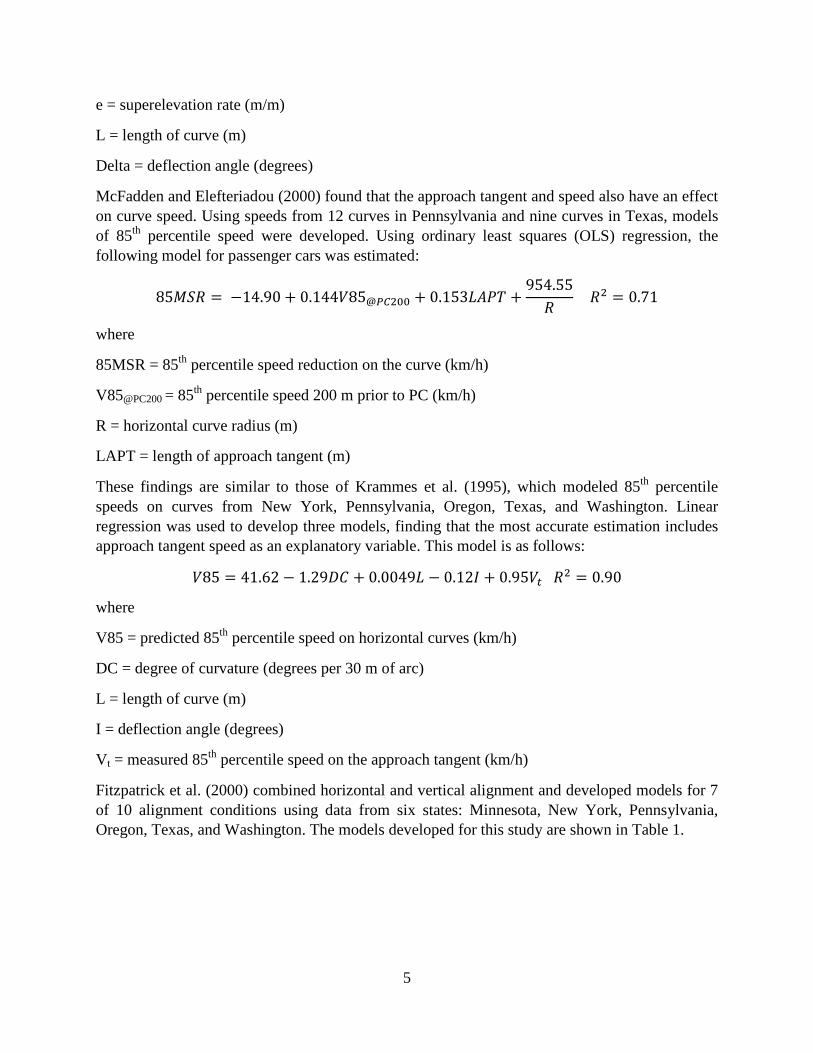
McFadden and Elefteriadou (2000) found that the approach tangent and speed also have an effect on curve speed. Using speeds from 12 curves in Pennsylvania and nine curves in Texas, models of 85th percentile speed were developed. Using ordinary least squares (OLS) regression, the following model for passenger cars was estimated:

85𝑀𝑀𝑅 = −14.90 + 0.144𝑉85@𝑃𝑃200 + 0.153𝐿𝐿𝐿𝐿 +954.55𝑅

𝑅2 = 0.71

where

85MSR = 85th percentile speed reduction on the curve (km/h)

V85@PC200 = 85th percentile speed 200 m prior to PC (km/h)

R = horizontal curve radius (m)

LAPT = length of approach tangent (m)

These findings are similar to those of Krammes et al. (1995), which modeled 85th percentile speeds on curves from New York, Pennsylvania, Oregon, Texas, and Washington. Linear regression was used to develop three models, finding that the most accurate estimation includes approach tangent speed as an explanatory variable. This model is as follows:

𝑉85 = 41.62 − 1.29𝐷𝐷 + 0.0049𝐿 − 0.12𝐼 + 0.95𝑉𝑡 𝑅2 = 0.90

where

V85 = predicted 85th percentile speed on horizontal curves (km/h)

DC = degree of curvature (degrees per 30 m of arc)

L = length of curve (m)

I = deflection angle (degrees)

Vt = measured 85th percentile speed on the approach tangent (km/h)

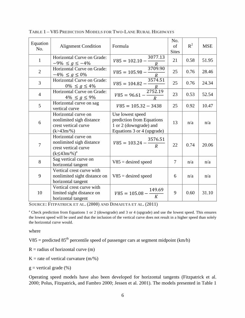
Fitzpatrick et al. (2000) combined horizontal and vertical alignment and developed models for 7 of 10 alignment conditions using data from six states: Minnesota, New York, Pennsylvania, Oregon, Texas, and Washington. The models developed for this study are shown in Table 1.

6

TABLE 1 – V85 PREDICTION MODELS FOR TWO-LANE RURAL HIGHWAYS

Equation No. Alignment Condition Formula

No. of

Sites R2 MSE

1 Horizontal Curve on Grade: −9% ≤ 𝑔 ≤ −4% 𝑉85 = 102.10 −

3077.13𝑅

21 0.58 51.95

2 Horizontal Curve on Grade: −4% ≤ 𝑔 ≤ 0% 𝑉85 = 105.98 −

3709.90𝑅

25 0.76 28.46

3 Horizontal Curve on Grade: 0% ≤ 𝑔 ≤ 4% 𝑉85 = 104.82 −

3574.51𝑅

25 0.76 24.34

4 Horizontal Curve on Grade: 4% ≤ 𝑔 ≤ 9% 𝑉85 = 96.61 −

2752.19𝑅

23 0.53 52.54

5 Horizontal curve on sag vertical curve 𝑉85 = 105.32 − 3438 25 0.92 10.47

6

Horizontal curve on nonlimited sigh distance crest vertical curve (k>43m/%)

Use lowest speed prediction from Equations 1 or 2 (downgrade) and Equations 3 or 4 (upgrade)

13 n/a n/a

7

Horizontal curve on nonlimited sigh distance crest vertical curve (k≤43m/%)a

𝑉85 = 103.24 −3576.51

𝑅

22 0.74 20.06

8 Sag vertical curve on horizontal tangent V85 = desired speed 7 n/a n/a

9 Vertical crest curve with nonlimited sight distance on horizontal tangent

V85 = desired speed 6 n/a n/a

10 Vertical crest curve with limited sight distance on horizontal tangent

𝑉85 = 105.08 −149.69𝐾

9 0.60 31.10

SOURCE: FITPATRICK ET AL. (2000) AND DIMAIUTA ET AL. (2011) a Check prediction from Equations 1 or 2 (downgrade) and 3 or 4 (upgrade) and use the lowest speed. This ensures the lowest speed will be used and that the inclusion of the vertical curve does not result in a higher speed than solely the horizontal curve would.

where

V85 = predicted 85th percentile speed of passenger cars at segment midpoint (km/h)

R = radius of horizontal curve (m)

K = rate of vertical curvature (m/%)

g = vertical grade (%)

Operating speed models have also been developed for horizontal tangents (Fitzpatrick et al. 2000; Polus, Fitzpatrick, and Fambro 2000; Jessen et al. 2001). The models presented in Table 1

7

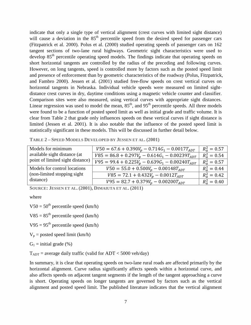
indicate that only a single type of vertical alignment (crest curves with limited sight distance) will cause a deviation in the 85th percentile speed from the desired speed for passenger cars (Fitzpatrick et al. 2000). Polus et al. (2000) studied operating speeds of passenger cars on 162 tangent sections of two-lane rural highways. Geometric sight characteristics were used to develop 85th percentile operating speed models. The findings indicate that operating speeds on short horizontal tangents are controlled by the radius of the preceding and following curves. However, on long tangents, speed is controlled more by factors such as the posted speed limit and presence of enforcement than by geometric characteristics of the roadway (Polus, Fitzpatrick, and Fambro 2000). Jessen et al. (2001) studied free-flow speeds on crest vertical curves on horizontal tangents in Nebraska. Individual vehicle speeds were measured on limited sight-distance crest curves in dry, daytime conditions using a magnetic vehicle counter and classifier. Comparison sites were also measured, using vertical curves with appropriate sight distances. Linear regression was used to model the mean, 85th, and 95th percentile speeds. All three models were found to be a function of posted speed limit as well as initial grade and traffic volume. It is clear from Table 2 that grade only influences speeds on these vertical curves if sight distance is limited (Jessen et al. 2001). It is also notable that the influence of the posted speed limit is statistically significant in these models. This will be discussed in further detail below.

TABLE 2 – SPEED MODELS DEVELOPED BY JESSEN ET AL. (2001)

Models for minimum available sight distance (at point of limited sight distance)

𝑉50 = 67.6 + 0.390𝑉𝑝 − 0.714𝐺1 − 0.0017𝐿𝐴𝐴𝑃 𝑅𝑎2 = 0.57 𝑉85 = 86.8 + 0.297𝑉𝑝 − 0.614𝐺1 − 0.00239𝐿𝐴𝐴𝑃 𝑅𝑎2 = 0.54 𝑉95 = 99.4 + 0.225𝑉𝑝 − 0.639𝐺1 − 0.00240𝐿𝐴𝐴𝑃 𝑅𝑎2 = 0.57

Models for control locations (non-limited stopping sight distance)

𝑉50 = 55.0 + 0.500𝑉𝑝 − 0.00148𝐿𝐴𝐴𝑃 𝑅𝑎2 = 0.44 𝑉85 = 72.1 + 0.432𝑉𝑝 − 0.0012𝐿𝐴𝐴𝑃 𝑅𝑎2 = 0.42 𝑉95 = 82.7 + 0.379𝑉𝑝 − 0.00200𝐿𝐴𝐴𝑃 𝑅𝑎2 = 0.40

SOURCE: JESSEN ET AL. (2001), DIMAIUTA ET AL. (2011)

where

V50 = 50th percentile speed (km/h)



Vp = posted speed limit (km/h)

G1 = initial grade (%)

TADT = average daily traffic (valid for ADT < 5000 veh/day)

In summary, it is clear that operating speeds on two-lane rural roads are affected primarily by the horizontal alignment. Curve radius significantly affects speeds within a horizontal curve, and also affects speeds on adjacent tangent segments if the length of the tangent approaching a curve is short. Operating speeds on longer tangents are governed by factors such as the vertical alignment and posted speed limit. The published literature indicates that the vertical alignment

8

only significantly affects operating speeds on limited sight distance vertical crest curves. Therefore, the posted speed limit is the primary factor that influences operating speeds on long tangent segments.

OPERATING SPEEDS ON MULTI-LANE HIGHWAYS Operating speed models also exist for multi-lane highways as discussed in the review by Dimaiuta et al. (2011), although attempts at modeling operating speeds on rural multi-lane highways are sparser than two-lane rural road studies. One study focused on the effect of speed limit increases on rural highways in Georgia following the repeal of the 55 mph National Maximum Speed Limit (Dixon et al. 1999). Analysis of speed and volume data collected before and after the change in speed limit from 55 mph to 65 mph revealed a 3.2 mph increase in mean operating speed. While this is a small increase, it was theorized that mean speed will continue to increase over time as drivers adjusted to the new posted speed limit.

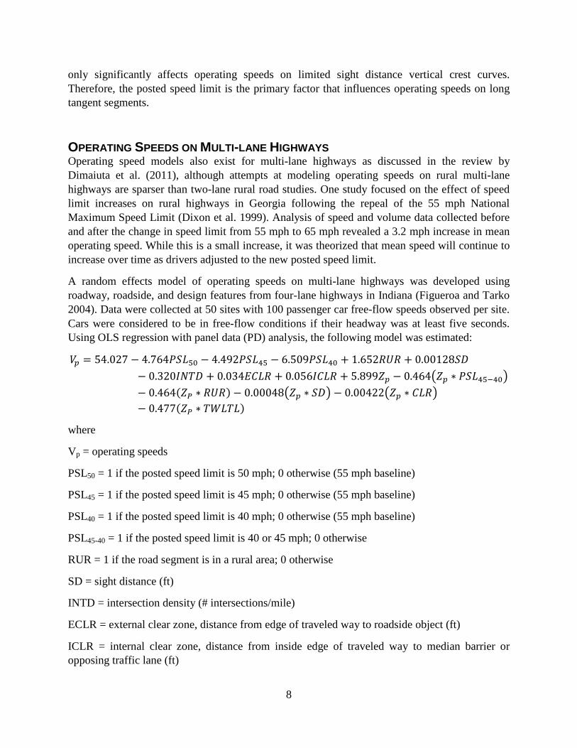
A random effects model of operating speeds on multi-lane highways was developed using roadway, roadside, and design features from four-lane highways in Indiana (Figueroa and Tarko 2004). Data were collected at 50 sites with 100 passenger car free-flow speeds observed per site. Cars were considered to be in free-flow conditions if their headway was at least five seconds. Using OLS regression with panel data (PD) analysis, the following model was estimated:

𝑉𝑝 = 54.027 − 4.764𝐿𝑀𝐿50 − 4.492𝐿𝑀𝐿45 − 6.509𝐿𝑀𝐿40 + 1.652𝑅𝑅𝑅 + 0.00128𝑀𝐷− 0.320𝐼𝐼𝐿𝐷 + 0.034𝐸𝐷𝐿𝑅 + 0.056𝐼𝐷𝐿𝑅 + 5.899𝑍𝑝 − 0.464�𝑍𝑝 ∗ 𝐿𝑀𝐿45−40�− 0.464(𝑍𝑃 ∗ 𝑅𝑅𝑅) − 0.00048�𝑍𝑝 ∗ 𝑀𝐷� − 0.00422�𝑍𝑝 ∗ 𝐷𝐿𝑅�− 0.477(𝑍𝑃 ∗ 𝐿𝑇𝐿𝐿𝐿)

where

Vp = operating speeds

PSL50 = 1 if the posted speed limit is 50 mph; 0 otherwise (55 mph baseline)



PSL45-40 = 1 if the posted speed limit is 40 or 45 mph; 0 otherwise

RUR = 1 if the road segment is in a rural area; 0 otherwise

SD = sight distance (ft)

INTD = intersection density (# intersections/mile)

ECLR = external clear zone, distance from edge of traveled way to roadside object (ft)

ICLR = internal clear zone, distance from inside edge of traveled way to median barrier or opposing traffic lane (ft)

9

Zp = standardize normal variable corresponding to a selected percentile speed

CLR = total clear zone (ICLR + ECLR, ft)

TWLTL = 1 of a two-way left-turn lane is present; 0 otherwise

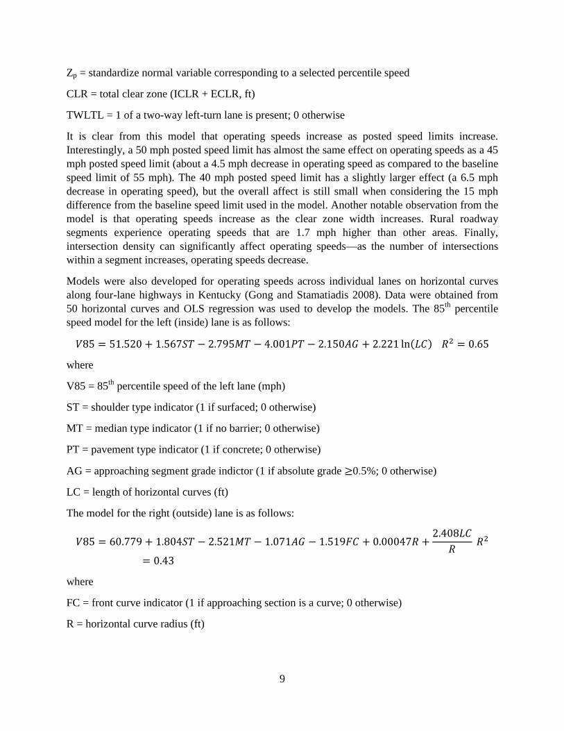
It is clear from this model that operating speeds increase as posted speed limits increase. Interestingly, a 50 mph posted speed limit has almost the same effect on operating speeds as a 45 mph posted speed limit (about a 4.5 mph decrease in operating speed as compared to the baseline speed limit of 55 mph). The 40 mph posted speed limit has a slightly larger effect (a 6.5 mph decrease in operating speed), but the overall affect is still small when considering the 15 mph difference from the baseline speed limit used in the model. Another notable observation from the model is that operating speeds increase as the clear zone width increases. Rural roadway segments experience operating speeds that are 1.7 mph higher than other areas. Finally, intersection density can significantly affect operating speeds—as the number of intersections within a segment increases, operating speeds decrease.

Models were also developed for operating speeds across individual lanes on horizontal curves along four-lane highways in Kentucky (Gong and Stamatiadis 2008). Data were obtained from 50 horizontal curves and OLS regression was used to develop the models. The 85th percentile speed model for the left (inside) lane is as follows:

𝑉85 = 51.520 + 1.567𝑀𝐿 − 2.795𝑀𝐿 − 4.001𝐿𝐿 − 2.150𝐿𝐺 + 2.221 ln(𝐿𝐷) 𝑅2 = 0.65

where

V85 = 85th percentile speed of the left lane (mph)

ST = shoulder type indicator (1 if surfaced; 0 otherwise)

MT = median type indicator (1 if no barrier; 0 otherwise)

PT = pavement type indicator (1 if concrete; 0 otherwise)

AG = approaching segment grade indictor (1 if absolute grade ≥0.5%; 0 otherwise)

LC = length of horizontal curves (ft)

The model for the right (outside) lane is as follows:

𝑉85 = 60.779 + 1.804𝑀𝐿 − 2.521𝑀𝐿 − 1.071𝐿𝐺 − 1.519𝐹𝐷 + 0.00047𝑅 +2.408𝐿𝐷

𝑅 𝑅2

= 0.43

where

FC = front curve indicator (1 if approaching section is a curve; 0 otherwise)

R = horizontal curve radius (ft)

10

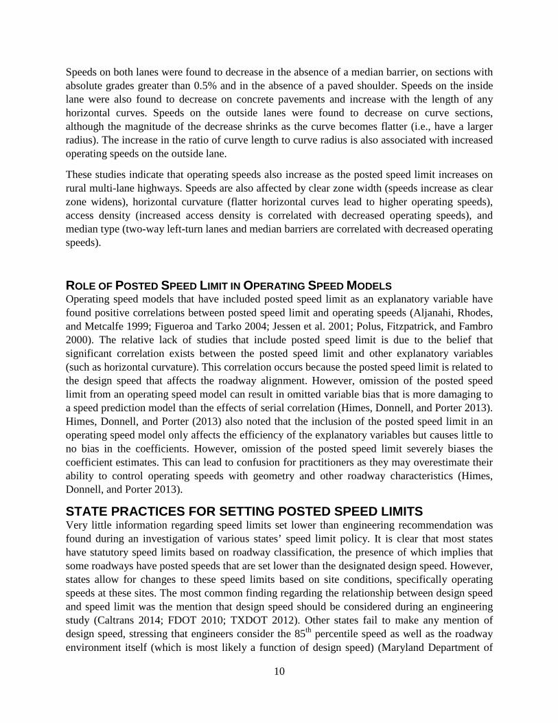
Speeds on both lanes were found to decrease in the absence of a median barrier, on sections with absolute grades greater than 0.5% and in the absence of a paved shoulder. Speeds on the inside lane were also found to decrease on concrete pavements and increase with the length of any horizontal curves. Speeds on the outside lanes were found to decrease on curve sections, although the magnitude of the decrease shrinks as the curve becomes flatter (i.e., have a larger radius). The increase in the ratio of curve length to curve radius is also associated with increased operating speeds on the outside lane.

These studies indicate that operating speeds also increase as the posted speed limit increases on rural multi-lane highways. Speeds are also affected by clear zone width (speeds increase as clear zone widens), horizontal curvature (flatter horizontal curves lead to higher operating speeds), access density (increased access density is correlated with decreased operating speeds), and median type (two-way left-turn lanes and median barriers are correlated with decreased operating speeds).

ROLE OF POSTED SPEED LIMIT IN OPERATING SPEED MODELS Operating speed models that have included posted speed limit as an explanatory variable have found positive correlations between posted speed limit and operating speeds (Aljanahi, Rhodes, and Metcalfe 1999; Figueroa and Tarko 2004; Jessen et al. 2001; Polus, Fitzpatrick, and Fambro 2000). The relative lack of studies that include posted speed limit is due to the belief that significant correlation exists between the posted speed limit and other explanatory variables (such as horizontal curvature). This correlation occurs because the posted speed limit is related to the design speed that affects the roadway alignment. However, omission of the posted speed limit from an operating speed model can result in omitted variable bias that is more damaging to a speed prediction model than the effects of serial correlation (Himes, Donnell, and Porter 2013). Himes, Donnell, and Porter (2013) also noted that the inclusion of the posted speed limit in an operating speed model only affects the efficiency of the explanatory variables but causes little to no bias in the coefficients. However, omission of the posted speed limit severely biases the coefficient estimates. This can lead to confusion for practitioners as they may overestimate their ability to control operating speeds with geometry and other roadway characteristics (Himes, Donnell, and Porter 2013).

STATE PRACTICES FOR SETTING POSTED SPEED LIMITS Very little information regarding speed limits set lower than engineering recommendation was found during an investigation of various states’ speed limit policy. It is clear that most states have statutory speed limits based on roadway classification, the presence of which implies that some roadways have posted speeds that are set lower than the designated design speed. However, states allow for changes to these speed limits based on site conditions, specifically operating speeds at these sites. The most common finding regarding the relationship between design speed and speed limit was the mention that design speed should be considered during an engineering study (Caltrans 2014; FDOT 2010; TXDOT 2012). Other states fail to make any mention of design speed, stressing that engineers consider the 85th percentile speed as well as the roadway environment itself (which is most likely a function of design speed) (Maryland Department of

11

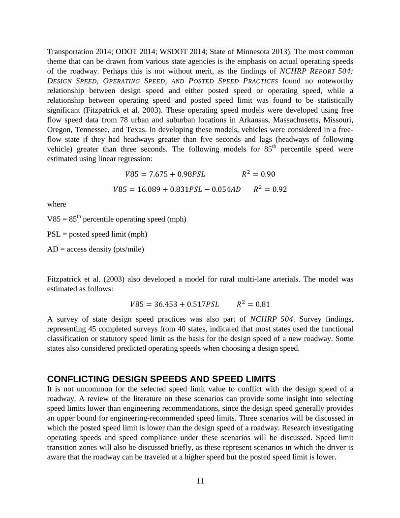
Transportation 2014; ODOT 2014; WSDOT 2014; State of Minnesota 2013). The most common theme that can be drawn from various state agencies is the emphasis on actual operating speeds of the roadway. Perhaps this is not without merit, as the findings of NCHRP REPORT 504: DESIGN SPEED, OPERATING SPEED, AND POSTED SPEED PRACTICES found no noteworthy relationship between design speed and either posted speed or operating speed, while a relationship between operating speed and posted speed limit was found to be statistically significant (Fitzpatrick et al. 2003). These operating speed models were developed using free flow speed data from 78 urban and suburban locations in Arkansas, Massachusetts, Missouri, Oregon, Tennessee, and Texas. In developing these models, vehicles were considered in a free-flow state if they had headways greater than five seconds and lags (headways of following vehicle) greater than three seconds. The following models for 85th percentile speed were estimated using linear regression:

𝑉85 = 7.675 + 0.98𝐿𝑀𝐿 𝑅2 = 0.90

𝑉85 = 16.089 + 0.831𝐿𝑀𝐿 − 0.054𝐿𝐷 𝑅2 = 0.92

where

V85 = 85th percentile operating speed (mph)

PSL = posted speed limit (mph)

AD = access density (pts/mile)

Fitzpatrick et al. (2003) also developed a model for rural multi-lane arterials. The model was estimated as follows:

𝑉85 = 36.453 + 0.517𝐿𝑀𝐿 𝑅2 = 0.81

A survey of state design speed practices was also part of NCHRP 504. Survey findings, representing 45 completed surveys from 40 states, indicated that most states used the functional classification or statutory speed limit as the basis for the design speed of a new roadway. Some states also considered predicted operating speeds when choosing a design speed.

CONFLICTING DESIGN SPEEDS AND SPEED LIMITS It is not uncommon for the selected speed limit value to conflict with the design speed of a roadway. A review of the literature on these scenarios can provide some insight into selecting speed limits lower than engineering recommendations, since the design speed generally provides an upper bound for engineering-recommended speed limits. Three scenarios will be discussed in which the posted speed limit is lower than the design speed of a roadway. Research investigating operating speeds and speed compliance under these scenarios will be discussed. Speed limit transition zones will also be discussed briefly, as these represent scenarios in which the driver is aware that the roadway can be traveled at a higher speed but the posted speed limit is lower.

12

NATIONAL MAXIMUM SPEED LIMIT One well-known example of a low posted speed limit is the implementation of the National Maximum Speed Limit (NMSL). In an effort to increase fuel efficiency and reduce oil usage during the oil embargo of the 1970’s, the U.S. federal government enacted legislation that established a maximum speed limit of 55 mph on all interstates (Friedman, Hedeker, and Richter 2009). This meant that many interstates built with design speeds of 70 mph, and previously operated with posted speed limits higher than 55 mph, were to enact a lower posted speed limit of 55 mph. Adhering to this speed limit was likely difficult for drivers for several reasons. First, these drivers likely had prior experience driving interstates at higher speeds, and thus would have felt comfortable driving at these speeds. Second, interstates were designed using uniform criteria that were the most “forgiving” (e.g., wider travel lanes, flatter horizontal curves) among criteria used for other roadway types. Due to this forgiving design, the inferred design speed of these facilities is likely much higher than 55 mph. This may confuse drivers as the roadway geometry provides no indication concerning compliance with the new posted speed limit of 55 mph.

Viewing speed limit compliance from a public policy standpoint, Meier and Morgan (1982) analyzed speed data from all 50 states to model the percent non-compliance based on environmental variables. Linear regression models were developed for two metrics: percent vehicles exceeding 55 mph (i.e., percent of non-compliance) and 85th percentile speed. Within a compliance theory framework, six variables were used to explain the speed variation of different states on NMSL facilities: miles driven per capita, size of the state (square miles), percent of interstate highways, days of precipitation, altitude variation, and minimum driving age. The first three variables were found to be positively correlated in both models, while the last three were negatively correlated. Residuals for each state were used to discuss a true level of non-compliance. Instead of simply viewing a state’s 85th percentile speed and percent of non-compliance on NMSL freeways, the authors suggest comparing the state’s metrics to those predicted by the models developed. States with highly positive residuals (i.e. those in which their actual speed metrics are much greater than those predicted) are those that had significant non-compliance issues with the NMSL. The data shows that Montana had a +3 percent residual for percent of vehicles exceeding a 55 mph speed limit and +0.93 mph residual for 85th percentile speed, suggesting non-compliance issues with respect to the NMSL (Meier and Morgan 1982). A similar national maximum speed limit exists in Israel (90 kilometers per hour or kph), and it is hypothesized that roughly half of the drivers exceed this limit (D. Shinar 2007). The NMSL is likely the best example of enforcing speed limits that are lower than design and engineering recommended speeds, and the framework of speed model residuals is described when discussing speed limit compliance.

WORK ZONE SPEED LIMITS Another common example of posted speed limits set lower than engineering recommendations occurs in work zones. Although work zone speed limits are temporary, vehicles often exceed them and travel at speeds near the permanent posted speed limit of the roadway. Research has shown that vehicles speeding prior to entering a work zone still travel at high speeds and violate the temporary speed limit, although they do reduce their speeds (Benekohal and Wang 1994).

13

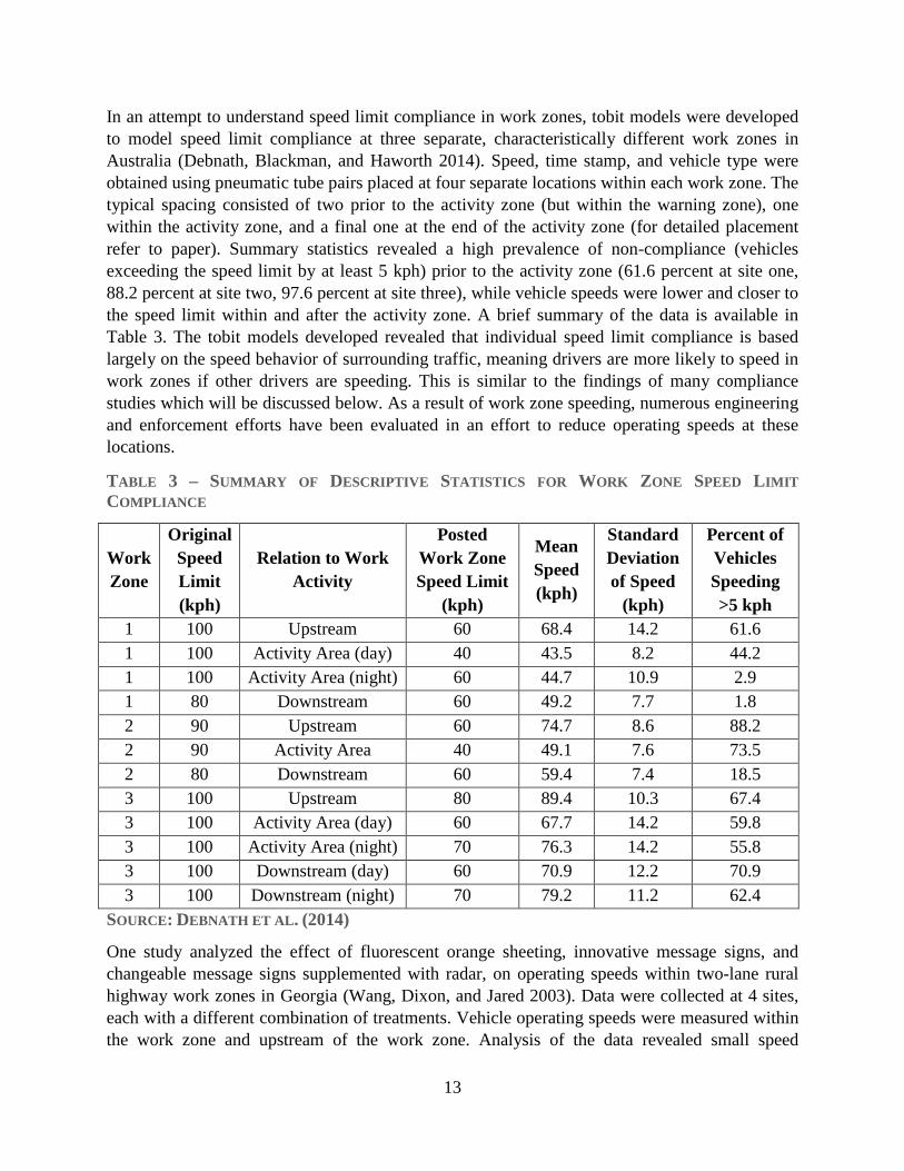
In an attempt to understand speed limit compliance in work zones, tobit models were developed to model speed limit compliance at three separate, characteristically different work zones in Australia (Debnath, Blackman, and Haworth 2014). Speed, time stamp, and vehicle type were obtained using pneumatic tube pairs placed at four separate locations within each work zone. The typical spacing consisted of two prior to the activity zone (but within the warning zone), one within the activity zone, and a final one at the end of the activity zone (for detailed placement refer to paper). Summary statistics revealed a high prevalence of non-compliance (vehicles exceeding the speed limit by at least 5 kph) prior to the activity zone (61.6 percent at site one, 88.2 percent at site two, 97.6 percent at site three), while vehicle speeds were lower and closer to the speed limit within and after the activity zone. A brief summary of the data is available in Table 3. The tobit models developed revealed that individual speed limit compliance is based largely on the speed behavior of surrounding traffic, meaning drivers are more likely to speed in work zones if other drivers are speeding. This is similar to the findings of many compliance studies which will be discussed below. As a result of work zone speeding, numerous engineering and enforcement efforts have been evaluated in an effort to reduce operating speeds at these locations.

TABLE 3 – SUMMARY OF DESCRIPTIVE STATISTICS FOR WORK ZONE SPEED LIMIT COMPLIANCE

Work Zone

Original Speed Limit (kph)

Relation to Work Activity

Posted Work Zone Speed Limit

(kph)

Mean Speed (kph)

Standard Deviation of Speed

(kph)

Percent of Vehicles Speeding >5 kph

1 100 Upstream 60 68.4 14.2 61.6 1 100 Activity Area (day) 40 43.5 8.2 44.2 1 100 Activity Area (night) 60 44.7 10.9 2.9 1 80 Downstream 60 49.2 7.7 1.8 2 90 Upstream 60 74.7 8.6 88.2 2 90 Activity Area 40 49.1 7.6 73.5 2 80 Downstream 60 59.4 7.4 18.5 3 100 Upstream 80 89.4 10.3 67.4 3 100 Activity Area (day) 60 67.7 14.2 59.8 3 100 Activity Area (night) 70 76.3 14.2 55.8 3 100 Downstream (day) 60 70.9 12.2 70.9 3 100 Downstream (night) 70 79.2 11.2 62.4

SOURCE: DEBNATH ET AL. (2014)

One study analyzed the effect of fluorescent orange sheeting, innovative message signs, and changeable message signs supplemented with radar, on operating speeds within two-lane rural highway work zones in Georgia (Wang, Dixon, and Jared 2003). Data were collected at 4 sites, each with a different combination of treatments. Vehicle operating speeds were measured within the work zone and upstream of the work zone. Analysis of the data revealed small speed

14

reductions (less than 3 mph) when fluorescent orange sheeting and innovative message signs were used. The novelty effect (i.e., adjustment of behavior based on the introduction of a new treatment) reduced the impact of the sheeting at some sites, while the innovative message signs failed to maintain any speed reduction. The biggest speed reduction was associated with changeable message signs with radar (CMSRs), which resulted in operating speed reductions up to 8 mph. A novelty effect was not found when using CMSRs in work zones. It should be noted that no information concerning the difference between work zone speed limit and upstream speed limit was made, meaning there is no context for viewing these speed reductions in terms of a change in the regulatory speed limit. It is clear from this study that speed compliance with signage is challenging, yet possible. General guidelines for the design of work zones, including discussion on speed enforcement, are discussed in NCHRP REPORT 581 (Mahoney et al. 2007).

SEASONAL SPEED LIMITS Another scenario that considers the impacts of speed limit reductions on vehicle operating speeds is the use of seasonal speed limits. Separate studies have investigated the effect of seasonal posted speed limit reductions in Finland. Finland has consistently experimented with lower winter speed limits from November to February with the goal of reducing crashes related to poor roadway conditions during the winter. Peltola (2000) found that a reduction of the speed limit from 100 km/h to 80 km/h using static speed limit signs reduced mean operating speeds of all vehicles by 3.8 km/h (compared to a 3.3 km/h reduction on control roads with no changed speed limit). Passenger car operating speeds were reduced by more than 5 km/h. Also, the variation in individual speeds was reduced, primarily at sites with higher posted speed limits. Data were obtained by measuring point speeds with radar at a set of locations per month for a two-year data collection period that began one month prior to the first speed limit reduction. Data collection resulted in 140,000 individual vehicle speed measurements. This study was performed using an observational before-after design with comparison sites using 100 treatment and 147 control sites (Peltola 2000).

Similarly, Rämä (2001) found a mean speed reduction of 3.4 km/h for a seasonal speed limit reduction of 120 km/h to 100 km/h using variable message speed limit signs, along with a reduction of speed variance. Speed data for this study were obtained using loop sensors. While both of these reductions were found to be statistically significant, the practical significance is nominal, considering the posted speed limit reduction was 20 km/h.

The studies discussed above reveal issues with speed limit compliance. It is clear that when faced with a reduced speed limit, drivers tend to disregard the lower posted speed limit if they feel like they can safely travel at a higher speed. This is likely due to previous safe navigating experience on this roadway and inferred design speed resulting from the characteristics of the roadway. One factor these studies did not consider is enforcement. The effect of enforcement is discussed in the next section, as well as how a driver chooses an operating speed and how speed limit compliance plays into this decision. These are discussed together because enforcement often influences speed choice.

15

SPEED LIMIT TRANSITION ZONES Speed transition zones are common on rural two-lane highways. These zones occur when a high-speed facility traverses through a town or area with many conflicts for which the original speed limit is no longer appropriate. NCHRP REPORT 737 provides design guidelines for agencies implementing high-to-low speed transition zones (Torbic et al. 2012). Research has demonstrated the factors that affect operating speed changes in transition zones (Cruzado and Donnell 2009; Cruzado and Donnell 2010). Cruzado and Donnell (2009) studied the effectiveness of dynamic speed display signs on free-flow operating speeds on two-lane rural highway transition zones in Pennsylvania. These signs consist of a speed limit sign and a dynamic message sign. The dynamic message sign reports the speed measured by the radar device to the driver of the oncoming vehicle, providing drivers with real-time feedback regarding their compliance. Data were collected before implementation, during implementation, and after the signs were removed. Analysis of the data revealed that dynamic speed display signs reduced operating speeds by about 6 mph during implementation, but this reduction diminished upon removal of the devices.

Cruzado and Donnell (2010) examined how various site characteristics affected speed reduction in transition zones on two-lane rural highways in Pennsylvania. 20 potential sites were identified based on the following criteria:

1. Presence of a Reduced Speed Ahead (W3-5) sign 2. No major signalized or stop-controlled intersections 3. Low percentage of heavy vehicles (less than 10 percent) 4. Low traffic volumes (to maximize free-flow observations) 5. Smooth pavement surface with good pavement markings

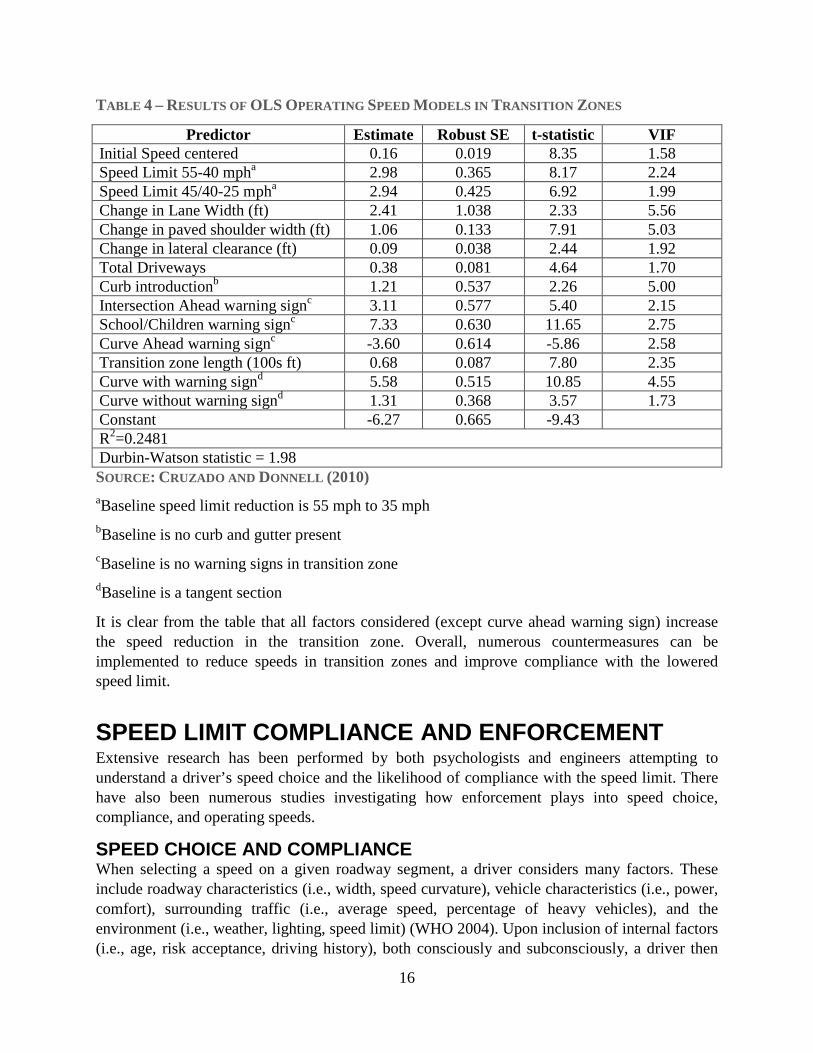
At each site, at least 100 free-flow vehicle observations were obtained from the following three locations: 500 feet prior to the Reduced Speed Ahead sign, at the Reduced Speed Ahead Sign, and at the lowered posted speed limit sign. Linear and multilevel regression models were used to predict speed reduction in the transition zone. Table 4 contains the results of the linear regression model.

16

TABLE 4 – RESULTS OF OLS OPERATING SPEED MODELS IN TRANSITION ZONES

Predictor Estimate Robust SE t-statistic VIF Initial Speed centered 0.16 0.019 8.35 1.58 Speed Limit 55-40 mpha 2.98 0.365 8.17 2.24 Speed Limit 45/40-25 mpha 2.94 0.425 6.92 1.99 Change in Lane Width (ft) 2.41 1.038 2.33 5.56 Change in paved shoulder width (ft) 1.06 0.133 7.91 5.03 Change in lateral clearance (ft) 0.09 0.038 2.44 1.92 Total Driveways 0.38 0.081 4.64 1.70 Curb introductionb 1.21 0.537 2.26 5.00 Intersection Ahead warning signc 3.11 0.577 5.40 2.15 School/Children warning signc 7.33 0.630 11.65 2.75 Curve Ahead warning signc -3.60 0.614 -5.86 2.58 Transition zone length (100s ft) 0.68 0.087 7.80 2.35 Curve with warning signd 5.58 0.515 10.85 4.55 Curve without warning signd 1.31 0.368 3.57 1.73 Constant -6.27 0.665 -9.43 R2=0.2481 Durbin-Watson statistic = 1.98 SOURCE: CRUZADO AND DONNELL (2010) aBaseline speed limit reduction is 55 mph to 35 mph bBaseline is no curb and gutter present cBaseline is no warning signs in transition zone dBaseline is a tangent section

It is clear from the table that all factors considered (except curve ahead warning sign) increase the speed reduction in the transition zone. Overall, numerous countermeasures can be implemented to reduce speeds in transition zones and improve compliance with the lowered speed limit.

SPEED LIMIT COMPLIANCE AND ENFORCEMENT Extensive research has been performed by both psychologists and engineers attempting to understand a driver’s speed choice and the likelihood of compliance with the speed limit. There have also been numerous studies investigating how enforcement plays into speed choice, compliance, and operating speeds.

SPEED CHOICE AND COMPLIANCE When selecting a speed on a given roadway segment, a driver considers many factors. These include roadway characteristics (i.e., width, speed curvature), vehicle characteristics (i.e., power, comfort), surrounding traffic (i.e., average speed, percentage of heavy vehicles), and the environment (i.e., weather, lighting, speed limit) (WHO 2004). Upon inclusion of internal factors (i.e., age, risk acceptance, driving history), both consciously and subconsciously, a driver then

17

selects a desired speed. While all of these factors play into speed choice, they affect the decision at different magnitudes. A survey conducted by the Transport Research Laboratory found that site characteristics had the biggest impact on a driver’s speed choice (Quimby et al. 1999). This is evidenced by the relationship between operating speeds and geometric characteristics previously shown in the operating speed models. Other research has found that an individual driver’s speed choice, especially in relation to a willingness to exceed the posted speed limit, is based largely on the speed of other vehicles (Haglund and Aberg 2000; C. Wang, Dixon, and Jared 2003). It has also been shown that drivers who have experience violating the speed limit are more likely to continue this behavior in the future as a result of developing a speeding habit (Elliott, Armitage, and Baughan 2003; De Pelsmacker and Janssens 2007). A more detailed discussion of this topic can be found in TRAFFIC SAFETY AND HUMAN BEHAVIOR (D. Shinar 2007).

ENFORCEMENT Speed enforcement is one of the few ways to ensure compliance with a posted speed limit. Most speed enforcement is performed by police officers, but some agencies utilize tools such as speed cameras.

Washington, D.C., implemented speed cameras mounted on police cruisers (Retting and Farmer 2003). These cameras use Doppler radar to monitor vehicle speeds and a violation of the speed limit triggers the camera to take a picture. 60 enforcement sites were identified, and from August 1 to October 1, speed cameras were deployed twice per week. Implementation of this program was preceded by a public awareness campaign and the enforcement sites were signed to warn drivers of the use of speed cameras. Seven of the 60 sites were randomly selected for the study, with eight similar comparison sites selected in Baltimore, Maryland. Speed data were collected using the speed camera equipment utilized by the police both before and after implementation. Analysis of the data revealed a statistically significant reduction in average speed of 14 percent and a reduction in non-compliance, compared to no reduction on the comparison sites.

A study of semi-rural highways in Canada by Hauer, Ahlin, and Bowser (1981) examined four enforcement scenarios using a single police car with radar in four separate field studies. Details of the four scenarios are shown in Table 5.

TABLE 5 – DESIGNS OF SPEED LIMIT ENFORCEMENT FIELD STUDIES

Experiment Number Visibility Days Enforced 1 Clear 1 2 Hidden 1 3 Hidden 5 4 Hidden 2 (with 3 days between)

SOURCE: HAUER, AHLIN, AND BOWSER (1981)

The “hidden” police vehicle was not visible by approaching vehicles until they were roughly 300 meters upstream. Speed data were collected for 2.5 hours per weekday for 5 weeks and measured at three locations: upstream, in front of the police cruiser, and roughly 2 km downstream.

18

Collection of data at these locations and time intervals also allowed the researchers to measure the impact of enforcement that persists upstream and downstream of the enforcement location (the distance halo effect) and after the enforcement period (the time halo effect) (Hauer, Ahlin, and Bowser 1981). The recorder also videotaped the rear of the car to record its license plate so the researchers could determine the effect of enforcement on both the overall speed distribution and for individual drivers. Analysis of the data indicated that all enforcement scenarios lowered average speed to near the posted speed limit at the location of enforcement. This speed reduction decayed exponentially as vehicles traveled away from the enforcement location in the downstream direction. Compliance with the speed limit also existed some distance upstream of the enforcement location, perhaps due to communication with the opposing traffic stream (e.g., flashing headlights). The impact of the time halo effect was related to the length of time enforcement was present. For instance, one day of enforcement reduced speeds for three days, while five days of enforcement reduced speeds for much longer.

Shinar and Stiebel (1986) compared the effect of stationary and moving police vehicles on speed limit compliance on a major Israeli freeway. This study, like the one completed by Hauer, Ahlin, and Bowser, recorded speeds upstream of the enforcement vehicle, at the enforcement vehicle, and downstream of the enforcement vehicle. Analysis of the data indicated that the presence of both police vehicle types reduced the speed of 95 percent of vehicles, and most reduced their speed to a value equal to or below the posted speed limit. Regression analysis revealed that both stationary and mobile police vehicles achieved the same compliance levels. However, the distance halo effect was found to be much more significant for moving police vehicles, as most vehicles that encountered the mobile cruiser were still traveling equal to or below the speed limit 4 km downstream, while the average operating speed of vehicles encountering the stationary vehicle returned to levels near their original operating speeds. A regression analysis confirmed that vehicles encountering the mobile cruiser recovered their original speed over a longer distance than those that encountered the stationary cruiser (David Shinar and Stiebel 1986).

The halo effect was also observed in another study performed in Norway, in which posted speed limits were enforced on a highway for an average of nine hours by a mix of stationary manned vehicles, mobile traffic surveillance, and a parked unmanned vehicle (Vaa 1997). The 5 weeks of enforcement in a 60 kph speed zone resulted in an eight week time halo during day-time hours (9am-3pm) while the 80 kph speed zone experienced a six week time halo during all hours except 6am-3pm. This study also found a statistically significant reduction in speeding vehicles, indicating a reduction in speed variance.

An observational before-after study of speed and safety on a 22 km long corridor of freeway in British Columbia was performed to estimate the effect of 12 stationary speed cameras (G. Chen, Meckle, and Wilson 2002). These speed cameras operated from 6 am to 11 pm and were programmed to photograph offenders violating the posted speed limit by greater than 11 kph. After collecting speed data from millions of vehicles using both the speed cameras and induction loops, it was found that mean speeds at individual speed camera locations dropped to or below the posted speed limit, while a speed reduction of more than 2 kph was found along the entire corridor. This indicates that these individual cameras have a significant distance halo.

19

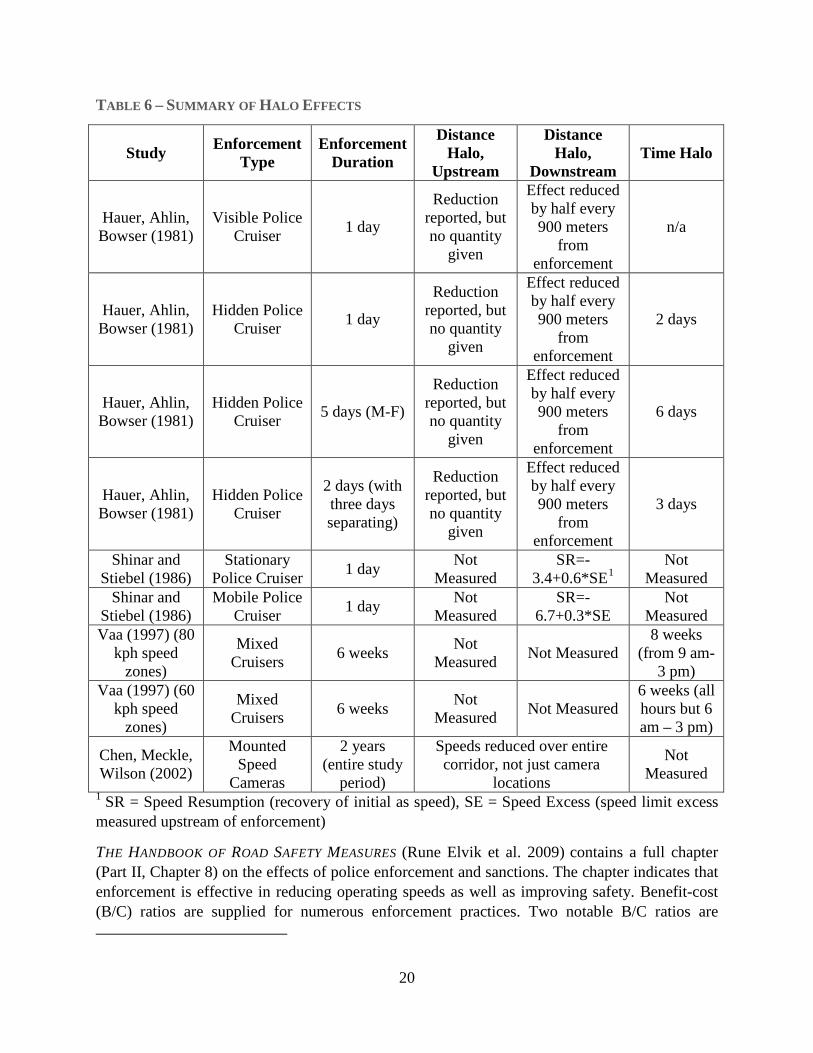
Researchers also found a statistically significant reduction of speed variance on the corridor of 0.5 (kph)2. Since enforcement was not removed, it was not possible to evaluate the existence of a time halo effect. However, the researchers noted that the drop in speed was consistent over the two year study period. An Empirical Bayes before-after study was also performed to determine the safety effect of the enforcement system. The results of this analysis found an expected crash reduction of 16 percent (standard deviation of 7 percent) over the entire corridor. A summary of the halo effects is shown in Table 6. Overall, it is clear that speed limit enforcement can reduce vehicle operating speeds to levels consistent with posted the speed limit. However, the distance and time halo effects indicate that the speed reduction is not permanent unless the enforcement is permanent (e.g., as would occur with speed cameras).

20

TABLE 6 – SUMMARY OF HALO EFFECTS

Study Enforcement Type

Enforcement Duration

Distance Halo,

Upstream

Distance Halo,

Downstream Time Halo

Hauer, Ahlin, Bowser (1981)

Visible Police Cruiser 1 day

Reduction reported, but no quantity

given

Effect reduced by half every 900 meters

from enforcement

n/a


Hidden Police Cruiser 1 day


given


from enforcement

2 days


Hidden Police Cruiser 5 days (M-F)


given


from enforcement

6 days


Hidden Police Cruiser

2 days (with three days separating)


given


from enforcement

3 days

Shinar and Stiebel (1986)

Stationary Police Cruiser 1 day Not

Measured SR=-

3.4+0.6*SE1 Not

Measured Shinar and

Stiebel (1986) Mobile Police

Cruiser 1 day Not Measured

SR=-6.7+0.3*SE

Not Measured

Vaa (1997) (80 kph speed

zones)

Mixed Cruisers 6 weeks Not

Measured Not Measured 8 weeks

(from 9 am-3 pm)

Vaa (1997) (60 kph speed

zones)

Mixed Cruisers 6 weeks Not

Measured Not Measured 6 weeks (all hours but 6 am – 3 pm)

Chen, Meckle, Wilson (2002)

Mounted Speed

Cameras

2 years (entire study

period)

Speeds reduced over entire corridor, not just camera

locations

Not Measured

1 SR = Speed Resumption (recovery of initial as speed), SE = Speed Excess (speed limit excess measured upstream of enforcement)

THE HANDBOOK OF ROAD SAFETY MEASURES (Rune Elvik et al. 2009) contains a full chapter (Part II, Chapter 8) on the effects of police enforcement and sanctions. The chapter indicates that enforcement is effective in reducing operating speeds as well as improving safety. Benefit-cost (B/C) ratios are supplied for numerous enforcement practices. Two notable B/C ratios are

21

tripling stationary speed enforcement (B/C = 1.5) and automatic speed enforcement (B/C ranges from 2 to 27). These indicate that typical enforcement strategies do see a return on investment mainly from safety benefits.

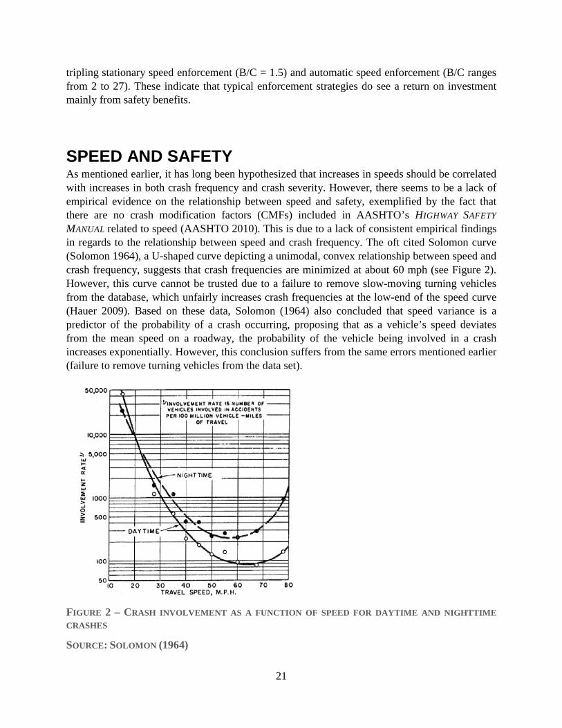
SPEED AND SAFETY As mentioned earlier, it has long been hypothesized that increases in speeds should be correlated with increases in both crash frequency and crash severity. However, there seems to be a lack of empirical evidence on the relationship between speed and safety, exemplified by the fact that there are no crash modification factors (CMFs) included in AASHTO’s HIGHWAY SAFETY MANUAL related to speed (AASHTO 2010). This is due to a lack of consistent empirical findings in regards to the relationship between speed and crash frequency. The oft cited Solomon curve (Solomon 1964), a U-shaped curve depicting a unimodal, convex relationship between speed and crash frequency, suggests that crash frequencies are minimized at about 60 mph (see Figure 2). However, this curve cannot be trusted due to a failure to remove slow-moving turning vehicles from the database, which unfairly increases crash frequencies at the low-end of the speed curve (Hauer 2009). Based on these data, Solomon (1964) also concluded that speed variance is a predictor of the probability of a crash occurring, proposing that as a vehicle’s speed deviates from the mean speed on a roadway, the probability of the vehicle being involved in a crash increases exponentially. However, this conclusion suffers from the same errors mentioned earlier (failure to remove turning vehicles from the data set).

FIGURE 2 – CRASH INVOLVEMENT AS A FUNCTION OF SPEED FOR DAYTIME AND NIGHTTIME CRASHES

SOURCE: SOLOMON (1964)

22

Abdel-Aty and Pande (2005) used real-time traffic data from a series of loop detectors on an urban freeway section to predict the probability of a crash occurring. Traffic data were averaged from over three lanes of traffic and divided into five-minute periods. Mean speed and standard deviation of the mean speed were determined for each five-minute period. A model for the probability of a crash occurring was developed using a neural network. The results indicated that crash propensity is the highest when mean speeds are low but the standard deviation of travel speeds is high. This is mainly due to the increased probability of rear end crashes in queuing scenarios. However, this and similar findings have been suggested to be an “ecological fallacy,” meaning aggregation of the data resulted in a misinterpreted relationship (Davis 2002). Reviewing the Solomon (1964) and Cirillo (1968) data, Davis (2002) and Hauer (2009) have questioned the validity of the U-shaped relationship between speed deviation and crash probability, raising concerns that speed variance does not necessarily predict crash frequency.

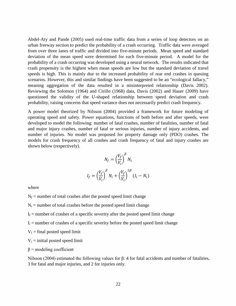
A power model theorized by Nilsson (2004) provided a framework for future modeling of operating speed and safety. Power equations, functions of both before and after speeds, were developed to model the following: number of fatal crashes, number of fatalities, number of fatal and major injury crashes, number of fatal or serious injuries, number of injury accidents, and number of injuries. No model was proposed for property damage only (PDO) crashes. The models for crash frequency of all crashes and crash frequency of fatal and injury crashes are shown below (respectively).

𝐼𝑓 = �𝑉𝑓𝑉𝑖�𝛽

𝐼𝑖

𝐼𝑓 = �𝑉𝑓𝑉𝑖�𝛽

𝐼𝑖 + �𝑉𝑓𝑉𝑖�2𝛽

(𝐼𝑖 − 𝐼𝑖)

where

Nf = number of total crashes after the posted speed limit change

Ni = number of total crashes before the posted speed limit change

If = number of crashes of a specific severity after the posted speed limit change

Ii = number of crashes of a specific severity before the posted speed limit change

Vf = final posted speed limit

Vi = initial posted speed limit

β = modeling coefficient

Nilsson (2004) estimated the following values for β: 4 for fatal accidents and number of fatalities, 3 for fatal and major injuries, and 2 for injuries only.

23

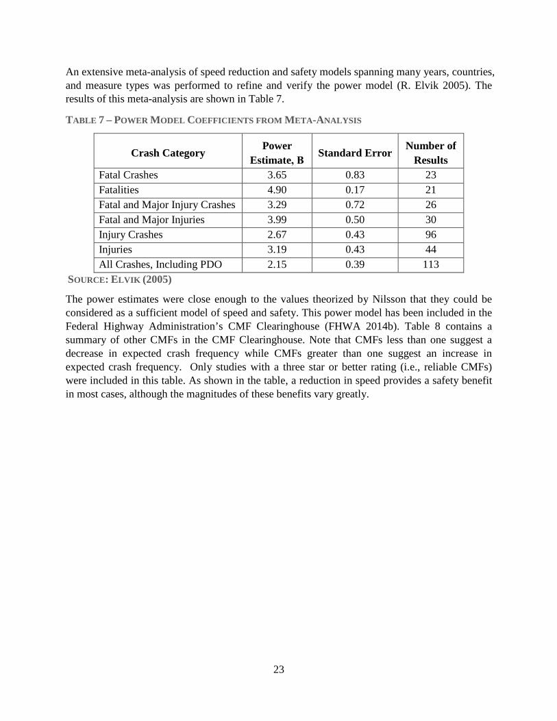
An extensive meta-analysis of speed reduction and safety models spanning many years, countries, and measure types was performed to refine and verify the power model (R. Elvik 2005). The results of this meta-analysis are shown in Table 7.

TABLE 7 – POWER MODEL COEFFICIENTS FROM META-ANALYSIS

Crash Category Power Estimate, Β Standard Error Number of

Results Fatal Crashes 3.65 0.83 23 Fatalities 4.90 0.17 21 Fatal and Major Injury Crashes 3.29 0.72 26 Fatal and Major Injuries 3.99 0.50 30 Injury Crashes 2.67 0.43 96 Injuries 3.19 0.43 44 All Crashes, Including PDO 2.15 0.39 113

SOURCE: ELVIK (2005)

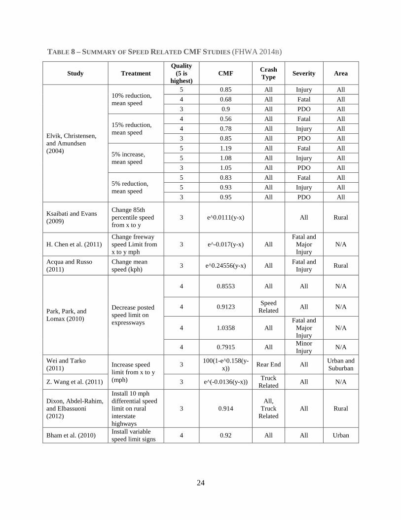
The power estimates were close enough to the values theorized by Nilsson that they could be considered as a sufficient model of speed and safety. This power model has been included in the Federal Highway Administration’s CMF Clearinghouse (FHWA 2014b). Table 8 contains a summary of other CMFs in the CMF Clearinghouse. Note that CMFs less than one suggest a decrease in expected crash frequency while CMFs greater than one suggest an increase in expected crash frequency. Only studies with a three star or better rating (i.e., reliable CMFs) were included in this table. As shown in the table, a reduction in speed provides a safety benefit in most cases, although the magnitudes of these benefits vary greatly.

24

TABLE 8 – SUMMARY OF SPEED RELATED CMF STUDIES (FHWA 2014B)

Study Treatment Quality

(5 is highest)

CMF Crash Type Severity Area

Elvik, Christensen, and Amundsen (2004)

10% reduction, mean speed

5 0.85 All Injury All 4 0.68 All Fatal All 3 0.9 All PDO All


4 0.56 All Fatal All 4 0.78 All Injury All 3 0.85 All PDO All

5% increase, mean speed




Ksaibati and Evans (2009)

Change 85th percentile speed from x to y

3 e^0.0111(y-x) All Rural

H. Chen et al. (2011) Change freeway speed Limit from x to y mph

3 e^-0.017(y-x) All Fatal and

Major Injury

N/A

Acqua and Russo (2011)

Change mean speed (kph) 3 e^0.24556(y-x) All Fatal and

Injury Rural

Park, Park, and Lomax (2010)

Decrease posted speed limit on expressways

4 0.8553 All All N/A

4 0.9123 Speed Related All N/A

4 1.0358 All Fatal and

Major Injury

N/A

4 0.7915 All Minor Injury N/A

Wei and Tarko (2011) Increase speed

limit from x to y (mph)

3 100(1-e^0.158(y-x)) Rear End All Urban and

Suburban

Z. Wang et al. (2011) 3 e^(-0.0136(y-x)) Truck Related All N/A

Dixon, Abdel-Rahim, and Elbassuoni (2012)

Install 10 mph differential speed limit on rural interstate highways

3 0.914 All,

Truck Related

All Rural

Bham et al. (2010) Install variable speed limit signs 4 0.92 All All Urban

25

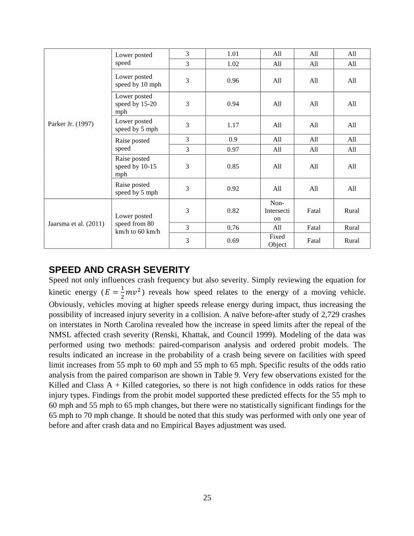
Parker Jr. (1997)

Lower posted speed

3 1.01 All All All 3 1.02 All All All

Lower posted speed by 10 mph 3 0.96 All All All

Lower posted speed by 15-20 mph

3 0.94 All All All

Lower posted speed by 5 mph 3 1.17 All All All

Raise posted speed

3 0.9 All All All 3 0.97 All All All

Raise posted speed by 10-15 mph

3 0.85 All All All

Raise posted speed by 5 mph 3 0.92 All All All

Jaarsma et al. (2011) Lower posted speed from 80 km/h to 60 km/h

3 0.82 Non-

Intersection

Fatal Rural

3 0.76 All Fatal Rural

3 0.69 Fixed Object Fatal Rural

SPEED AND CRASH SEVERITY Speed not only influences crash frequency but also severity. Simply reviewing the equation for kinetic energy (𝐸 = 1

2𝑚𝑣2 ) reveals how speed relates to the energy of a moving vehicle.

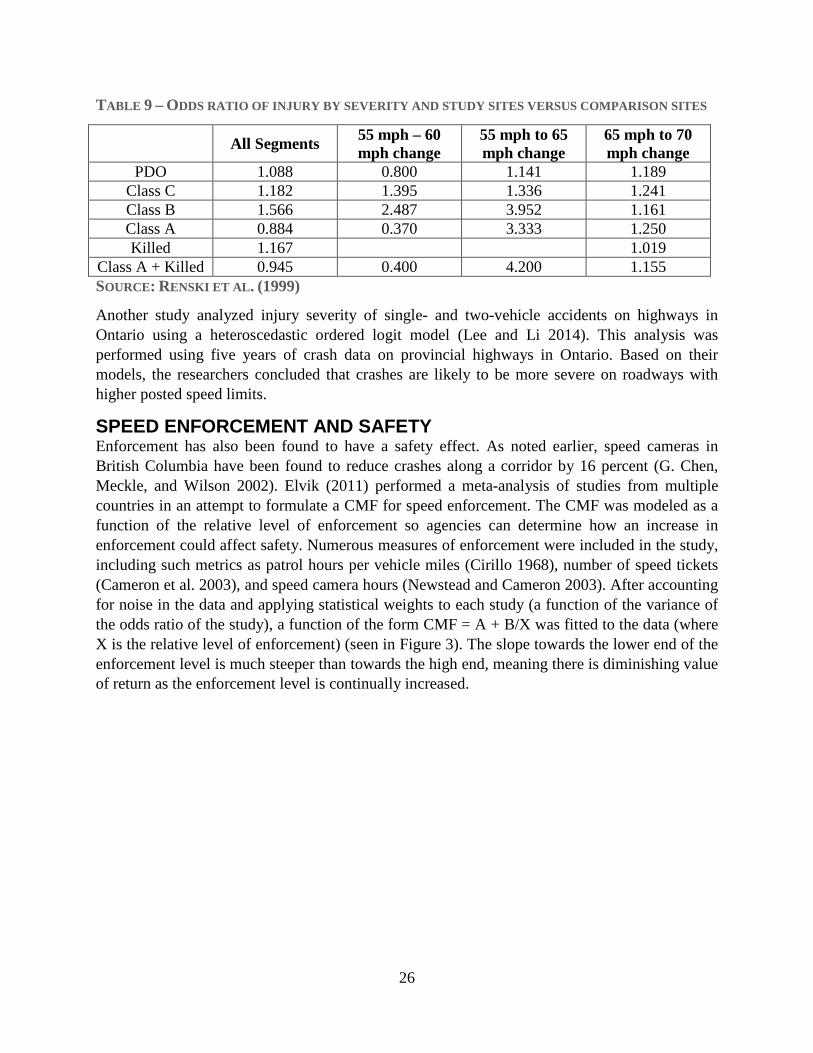
Obviously, vehicles moving at higher speeds release energy during impact, thus increasing the possibility of increased injury severity in a collision. A naïve before-after study of 2,729 crashes on interstates in North Carolina revealed how the increase in speed limits after the repeal of the NMSL affected crash severity (Renski, Khattak, and Council 1999). Modeling of the data was performed using two methods: paired-comparison analysis and ordered probit models. The results indicated an increase in the probability of a crash being severe on facilities with speed limit increases from 55 mph to 60 mph and 55 mph to 65 mph. Specific results of the odds ratio analysis from the paired comparison are shown in Table 9. Very few observations existed for the Killed and Class A + Killed categories, so there is not high confidence in odds ratios for these injury types. Findings from the probit model supported these predicted effects for the 55 mph to 60 mph and 55 mph to 65 mph changes, but there were no statistically significant findings for the 65 mph to 70 mph change. It should be noted that this study was performed with only one year of before and after crash data and no Empirical Bayes adjustment was used.

26

TABLE 9 – ODDS RATIO OF INJURY BY SEVERITY AND STUDY SITES VERSUS COMPARISON SITES

All Segments 55 mph – 60 mph change

55 mph to 65 mph change

65 mph to 70 mph change

PDO 1.088 0.800 1.141 1.189 Class C 1.182 1.395 1.336 1.241 Class B 1.566 2.487 3.952 1.161 Class A 0.884 0.370 3.333 1.250 Killed 1.167 1.019

Class A + Killed 0.945 0.400 4.200 1.155 SOURCE: RENSKI ET AL. (1999)

Another study analyzed injury severity of single- and two-vehicle accidents on highways in Ontario using a heteroscedastic ordered logit model (Lee and Li 2014). This analysis was performed using five years of crash data on provincial highways in Ontario. Based on their models, the researchers concluded that crashes are likely to be more severe on roadways with higher posted speed limits.

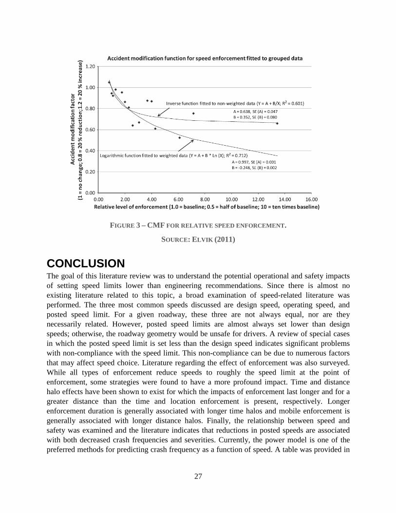
SPEED ENFORCEMENT AND SAFETY Enforcement has also been found to have a safety effect. As noted earlier, speed cameras in British Columbia have been found to reduce crashes along a corridor by 16 percent (G. Chen, Meckle, and Wilson 2002). Elvik (2011) performed a meta-analysis of studies from multiple countries in an attempt to formulate a CMF for speed enforcement. The CMF was modeled as a function of the relative level of enforcement so agencies can determine how an increase in enforcement could affect safety. Numerous measures of enforcement were included in the study, including such metrics as patrol hours per vehicle miles (Cirillo 1968), number of speed tickets (Cameron et al. 2003), and speed camera hours (Newstead and Cameron 2003). After accounting for noise in the data and applying statistical weights to each study (a function of the variance of the odds ratio of the study), a function of the form CMF = A + B/X was fitted to the data (where X is the relative level of enforcement) (seen in Figure 3). The slope towards the lower end of the enforcement level is much steeper than towards the high end, meaning there is diminishing value of return as the enforcement level is continually increased.

27

FIGURE 3 – CMF FOR RELATIVE SPEED ENFORCEMENT.

SOURCE: ELVIK (2011)

CONCLUSION The goal of this literature review was to understand the potential operational and safety impacts of setting speed limits lower than engineering recommendations. Since there is almost no existing literature related to this topic, a broad examination of speed-related literature was performed. The three most common speeds discussed are design speed, operating speed, and posted speed limit. For a given roadway, these three are not always equal, nor are they necessarily related. However, posted speed limits are almost always set lower than design speeds; otherwise, the roadway geometry would be unsafe for drivers. A review of special cases in which the posted speed limit is set less than the design speed indicates significant problems with non-compliance with the speed limit. This non-compliance can be due to numerous factors that may affect speed choice. Literature regarding the effect of enforcement was also surveyed. While all types of enforcement reduce speeds to roughly the speed limit at the point of enforcement, some strategies were found to have a more profound impact. Time and distance halo effects have been shown to exist for which the impacts of enforcement last longer and for a greater distance than the time and location enforcement is present, respectively. Longer enforcement duration is generally associated with longer time halos and mobile enforcement is generally associated with longer distance halos. Finally, the relationship between speed and safety was examined and the literature indicates that reductions in posted speeds are associated with both decreased crash frequencies and severities. Currently, the power model is one of the preferred methods for predicting crash frequency as a function of speed. A table was provided in

28

which speed-related crash modification factors from the CMF Clearinghouse were explained. Finally, the safety benefits of enforcement were covered.

The findings of this literature review will assist in the development of the data collection plan. Free-flow speed studies seem to be the main tool for assessing operating speeds on a facility. Speeds in these studies can be measured using various tools including radar, pneumatic road tubes, and on-pavement sensors. Previous studies indicate that a vehicle is in “free-flow” conditions if its lead headway is at least five seconds and a trail headway of three seconds. The operating speed models discussed suggest that posted speed limits, design speed, and geometry impact operating speeds. Therefore, when searching for comparison sites, roadways should be similar in these characteristics as well as similar engineering recommended speeds.

Based on the findings of this literature review, it is likely that there is a somewhat significant level of non-compliance on roadways with posted speed limits lower than the engineering recommended speed. A free-flow speed study will likely reveal an 85th percentile speed that is significantly larger than the speed limit. These high speeds will likely cause safety problems, especially considering the high level of non-compliance. In order to account for this, enforcement strategies that maximize distance and time halos should be considered.

29

REFERENCES AASHTO (American Association of State Highway Transportation Officials), Highway Safety

Manual 1st Edition. American Association of State Highway Transportation Officials (2010).

AASHTO (American Association of State Highway Transportation Officials), A Policy on the Geometric Design of Highways and Streets. American Association of State Highway Transportation Officials (2011) pp. 1.1-10.132.

Abdel-Aty, M. and Pande, A., “Identifying Crash Propensity Using Specific Traffic Speed Conditions.” Journal of Safety Research, Vol. 36 (2005) pp. 97-108.

Acqua, G. D. and Russo, F., “Safety Performance Functions for Low-Volume Roads.” 90th Annual Meeting of the Transportation Research Board, Washington, D.C. (2011).

Ahlin, F. J. “An Investigation in the Consistency of Driver’s Speed Choice.” Doctoral Dissertation, University of Toronto, Toronto, ON. (1979).

Aljanahi, A. A. M., Rhodes, A. H., and Metcalde, A. V., “Speed, Speed Limits and Road Traffic Accidents under Free Flow Conditions.” Accident Analysis & Prevention, Vol. 31, Nos. 1-2 (1999) pp. 161-168.

Benekohal, R. F. and Wang, L., “Relationship between Initial Speed and Speed inside a Highway Work Zone.” Transportation Research Record: Journal of the Transportation Research Board 1441 (1994) pp. 41-48.

Bham, G. H., Long, S., Baik, H., Ryan, T., Gentry, L., Lall, K., Arezoumandi, M., Liu, D., Li, T., and Schaeffer, B., “Evaluation of Variable Speed Limits on I-270/I-255 in St. Louis”. TRyy0825, RI 08‐025, Missouri Department of Transportation, Rolla, MO (2010) pp. 1-39.

Caltrans, “2014 California Manual for Setting Speed Limits.” California Department of Transportation (2014) pp. 1-91.

Cameron, M. H., Newstead, S., Diamantopoulou, K., and Oxley, P., “The Interaction between Speed Camera Enforcement and Speed-Related Mass Media Publicity in Victoria.” 47th Annual Proceedings of the Association for the Advancement of Automotive Medicine, Lisbon, Portugal (2003) pp. 267-282.

Chen, H., Zhang, Y., Wang, Z., and Lu, J., “Identifying Crash Distributions and Prone Locations by Lane Groups at Freeway Diverging Areas.” Accident Analysis & Prevention, Vol. 32, No. 2 (2002) pp. 129-138.

Cirillo, J. A. “Interstate System Accident Research Study II, Interim Report II.” Public Roads, Vol. 35, No. 3 (1968) pp. 71-75.

30

Cruzado, I. and Donnell, E. T., “Evaluating Effectiveness of Dynamic Speed Display Signs in Transition Zones of Two-Lane Rural Highways in Pennsylvania.” Transportation Research Record: Journal of the Transportation Research Board 2112 (2009) pp. 1-8.

Cruzado, I. and Donnell, E. T., “Factors Affecting Driver Speed Choice along Two-Lane Rural Highway Transition Zones.” Journal of Transportation Engineering, Vol. 136, No. 8 (2010) pp. 755-764.

Davis, G. A., “Is the Claim that ‘Variance Kills’ an Ecological Fallacy?” Accident Analysis & Prevention, Vol. 32, No. 3 (2002) pp. 343-346.

De Pelsmacker, P., and Janssens, W., “The Effect of Norms, Attitudes and Habits on Speeding Behavior: scale Development and Model Building Estimation.” Accident Analysis & Prevention, Vol. 39, No. 1 (2007) pp. 6-15.

Debnath, A. K., Blackman, R., and Haworth, N. “A Tobit Model for Analyzing Speed Limit Compliance in Work Zones.” Safety Science, Vol. 70, December (2014) pp. 367-377.

Dimaiuta, M., Donnell, E. T., Himes, S. C., and Porter, R. J., “Speed Models in North America.” TRB E-Circular 151 – Modeling Operating Speed: Synthesis Report, Washington, D.C., Transportation Research Board, National Research Council (2011) pp. 3-42.

Dixon, K. K., Wu, C. H., Sarasua, W., and Daniels, J., “Posted and Free-Flow Speeds for Rural Multilane Highways in Georgia.” Journal of Transportation Engineering, Vol. 125, No. 6 (1999) pp. 487-494.

Donnell, E. T., Himes, S. C., Mahoney, K. M., Porter, R. J., and McGee, H., “Speed Concepts: Informational Guide.” FHWA-SA-10-001, Federal Highway Administration, U.S. Department of Transportation, Washington, D.C. (2009) pp. 1-50.

Donnell, E. T., Ni, Y., Adolini, M., Eleferiadou, L., “Speed Prediction Models for Trucks on Two-Lane Rural Highways.” Transportation Research Record: Journal of the Transportation Research Board 1751, (2001) pp. 44-55.

Elliot, M. A., Armitage, C. J., Baughan, C. J., “Drivers’ Compliance with Speed Limits: An Application of the Theory of Planned Behavior.” The Journal of Applied Psychology, Vol. 88, No. 5 (2003) pp. 964-972.

Elvik, R., “Speed and Road Safety: Synthesis of Evidence from Evaluation Studies.” Transportation Research Record: Journal of the Transportation Research Board 1908, (2005) pp. 59-69.

Elvik, R., Christensen, P., Amundsen, A., “Speed and Road Accidents: An Evaluation of the Power Model.” TØI report 740, Transportokonomisk Institutt, Oslo, Norway (2004) pp. 1-134.

Elvik, R., Hoye, A., Vaa, T., and Sorensen, M., The Handbook of Road Safety Measures. Emerald Group Publishing Limited, Bingley, U.K. (2009) 2nd Edition pp. 1-1124

31

FDOT (Florida Department of Transportation), “Speed Zoning for Highways, Roads and Streets in Florida.” Topic No. 750-010-002, Traffic Engineering & Operations Office, Florida Department of Transportation, Tallahassee, FL (2010) pp. 1.1-16.6.

FHWA (Federal Highway Administration), USLIMITS2: A Web-Based Tool for Setting Appropriate Speed Limits. Washington, D.C.: Federal Highway Administration, U.S. Department of Transportation, (2014a). Informational flyer. http://safety.fhwa.dot.gov/uslimits/documents/uslimits2_flyer_lowres121012.pdf

FHWA (Federal Highway Administration), CMF Clearinghouse.” (2014b) hhtp://www.cmfclearinghouse.org/index.cfm. Accessed: 10/1/2014

Figueroa, A. and Tarko, A., “Reconciling Speed Limits with Design Speeds.” Report No. FHWA/IN/JTRP-2004/26, Purdue University, West Lafayette, Ind. (2004) pp. 1-165.

Fitzpatrick, K., Carlson, P., Brewer, M. A., Wooldridge, M. D., and Miaou, S., “Design Speed, Operating Speed, and Posted Speed Practices.” NCHRP Report 504, Transportation Research Board, National Research Council, Washington, D.C. (2003) pp. 1-92.

Fitzpatrick, K., Elefteriadou, L., Harwood, D. W., Collins, J., McFadden, J., Anderson, I. B., Krammes, R. A., Irizarry, N., Parma, K., Bauer, K. M., Passetti, K., “Speed Prediction Models for Two-Lane Rural Highways.” Report FHWA-RD-99-171, Federal Highway Administration, U.S. Department of Transportation, Washington, D.C. (2000) pp. 1-213.

Forbes, G. J., Gardner, T., McGee, H., and Srinivasan, R., “Methods and Practices for Setting Speed Limits.” FHWA-SA-12-004, Federal Highway Administration, U.S. Department of Transportation, Washington, D.C. (2012) pp. 1-109.

Friedman, L. S., Hedeker, D., and Richter, E. D., “Long-Term Effects of Repealing the National Maximum Speed Limit in the United States.” American Journal of Public Health, Vol. 99, No. 9 (2009) pp. 1626-1631.

Gong, H. and Stamatiadis, N., “Operating Speed Prediction Models for Horizontal Curves on Rural Four-Lane Highways.” 87th Annual Meeting of the Transportation Research Board, Washington, D.C., (2008).

Haglund, M. and Aberg, L., “Speed Choice in Relation to Speed Limit and Influences from Other Drivers.” Transportation Research Part F: Traffic Psychology and Behavior 3 (2000) pp. 39-51.

Hauer, E., “Speed and Safety.” Transportation Research Record: Journal of the Transportation Research Board 2103 (2009) pp. 10-17.

Hauer, E., Ahlin, F. J., and Bowser, J. S., “Speed Enforcement and Speed Choice.” Accident Analysis & Prevention, Vol. 14, No. 4 (1981) pp. 267-278.

Himes, S. C., Donnell, E. T., and Porter, R. J., “Posted Speed Limit: To Include or Not to Include in Operating Speed Models.” Transportation Research Part A: Policy and Practice 52 (2013) pp. 23-33.

32

Institute of Transportation Engineers, Manual of Transportation Engineering Studies. Prentice Hall, Englewood (2010) 2nd Edition pp. 1-514

Islam, M. N. and Seneviratne, P. N., “Evaluation of Design Consistency of Two-Lane Rural Highways.” ITE Journal, Vol. 64, No. 2 (1994) pp. 28-31.

Jaarsma, R., Louwerse, R., Dijkstra, A., and de Vries, J., “Making Minor Rural Road Networks Safer: The Effects of 60 km/h-Zones.” Accident Analysis & Prevention, Vol. 43, No. 4 (2011) pp. 1508-1515.

Jessen D. R., Schurr, K. S., McCoy, P.T., Pesti, G., and Huff, R. R., “Operating Speed Prediction on Crest Vertical Curves of Rural Two-Lane Highways in Nebraska.” Transportation Research Record: Journal of the Transportation Research Board 1751 (2001) pp. 67-75.

Krammes, R. A., Brackett, R. Q., Shafer, M. A., Ottesen, J. L., Anderson, I. B., Fink, K. L., Collins, K. M., Pendleton, O. J., and Messer, C. J., “Horizontal Alignment Design Consistency for Rural Two-Lane Highways.” Report No. FHWA-RD-94-034, Federal Highway Administration, U.S. Department of Transportation, Washington, D.C. (1995) pp. 1-127.

Ksaibati, K. and Evans, B., “WRRSP: Wyoming Rural Road Safety Program.” FHWA-WY-09/06F, Wyoming Department of Transportation, Federal Highway Administration, U.S. Department of Transportation, Washington, D.C. (2009) pp.1-272.

Lee, C. and Li, X., “Analysis of Injury Severity of Drivers Involved in Single- and Two-Vehicle Crashes on Highways in Ontario.” Accident Analysis & Prevention, Vol. 71, October (2014) pp. 286-295.

Mahoney, K. M., Porter, R. J., Taylor, D. R., and Kulakowski, B. R., “Design of Construction Work Zones.” NCHRP Report 581, Transportation Research Board, National Research Council, Washington, D.C. (2007) pp. 1-65.

Maryland Department of Transportation, “Speed Limits.” (2014) http://www.sha.maryland.gov/Index.aspx?PageId=295. Accessed: 10/1/2014.

McFadden, J. and Elefteriadou, L., “Evaluating Horizontal Alignment Design Consistency of Two-Lane Rural Highways.” Transportation Research Record: Journal of the Transportation Research Board 1737 (2000) pp. 9-16.

McFadden, J., Yang, W. T., and Durrans, S. R., “Application of Artificial Networks to Predict Speeds on Two-Lane Rural Highways.” Transportation Research Record: Journal of the Transportation Research Board 1751 (2001) pp. 9-17.

Meier, K. J. and Morgan, D. R., “Citizen Compliance with Public Policy: The National Maximum Speed Law.” The Western Political Quarterly, Vol. 35, No. 2 (1982) pp. 258-273.

33

Misaghi, P. and Hassan, Y., “Modeling Operating Speed and Speed Differential on Two-Lane Rural Roads.” Journal of Transportation Engineering, Vol. 131, No. 6 (2005) pp. 408-417.

Newstead, S. and Cameron, M. H., “Evaluation of the Crash Effects of the Queensland Speed Camera Program.” Report 204, Monash University Accident Research Centre, Victoria, Australia (2003) pp. 1-35.

Nilsson, G., “An Investigation in the Consistency of Driver’s Speed Choice.” Doctoral Dissertation, Lund Institute of Technology, Lund, Sweden (2004).

ODOT (Ohio Department of Transportation), “Speed Zones – Ohio Speed Limits.” (2014) http://www.dot.state.oh.us/districts/D01/PlanningPrograms/trafficstudies/SpeedZoens/Pages/default.aspx Accessed: 10/1/2014

Park, E. S., Park, J., and Lomax, T. J., “A Fully Bayesian Multivariate Approach to Before-After Safety Evaluation.” Accident Analysis & Prevention, Vol. 42, No. 4 (2010) pp. 1118-1127.

Parker, M. R., “Effects of Raising and Lowering Speed Limits on Selected Roadway Sections.” No. FHWA-RD-92-084, Federal Highway Administration, U.S. Department of Transportation, Washington, D.C. (1997) pp. 1-166.

Peltola, H., “Seasonally Changing Speed Limits Effects on Speeds and Accidents.” Transportation Research Record: Journal of the Transportation Research Board 1734, (2000) pp. 46-51.

Poe, C. M., Tarris, J. P., and Mason Jr., J. M., “Operating Speed Approach to Geometric Design of Low-Speed Urban Streets.” Report Number PTI 9606, Pennsylvania Transportation Institute, Penn State University, University Park, PA (1996) pp. 10.1-10.9.

Polus, A., Fitzpatrick, K., and Fambro, D. B., “Predicting Operating Speeds on Tangent Sections of Two-Lane Rural Highways.” Transportation Research Record: Journal of the Transportation Research Board 1737 (2000) pp.50-57.

Quimby, A., Maycock, G., Palmer, C., and Buttress, S., “The Factors That Influence a Driver’s Choice of Speed – A Questionnaire Study.” TRL Report 325, Transport Research Laboratory, U.K. (1999) pp. 1-34.

Rämä, P., “Effects of Weather-Controlled Variable Message Signing on Driver Behaviour.” Doctoral Dissertation, VTT Technical Research Centre of Finland, Helsinki University of Technology, Helsinki, Finland (2004) pp.1-55.

Renski, H., Khattak, A. J., Council, F. M., “Effects of Speed Limit Increases on Crash Injury Severity: Analysis of Single-Vehicle Crashes on North Carolina Interstate Highways.” Transportation Research Record: Journal of the Transportation Research 1665 (1999) pp. 100-108.

34

Retting, R. A. and Farmer, C. M., “Evaluation of Speed Camera Enforcement in the District of Columbia.” Transportation Research Record: Journal of the Transportation Research Board 1830 (2003) pp. 34-37.

Shinar, D., Traffic Safety and Human Behavior. Emerald Group Publishing Limited, Bingley, U.K. (2007) 2nd Edition pp. 1-776.

Shinar, D. and Stiebel, J., “The Effectiveness of Stationary versus Moving Police Vehicles on Compliance with Speed Limit.” Human Factors: The Journal of the Human Factors and Ergonomics Society, Vol. 28, No. 3 (1986) pp. 365-371.

Solomon, D., “Accidents on Main Rural Highways Related to Speed, Driver, and Vehicle.” (1964) pp. 1-44.

State of Minnesota, “2013 Minnesota Statutes.” The Office of the Revisor of Statutes. (2013) http://www.revisor.mn.gov/statutes/?id=169.14 Accessed: 10/1/2014.

Torbic, D. J., Gilmore, D. K., Bauer, K. M., Bokenroger, C. D., Harwood, D. W., Lucas, L. M., Frazier, R. J., Kinzel, C. S., Petree, D. L., and Forsberg, M. D., “Design Guidance for High-Speed to Low-Speed Transition Zones for Rural Highways.” NCHRP Report 737, Transportation Research Board, National Research Council, Washington, D.C. (2012) pp. 1-88.

Transportation Research Board, Managing Speed: Review of Current Practice for Setting and Enforcing Speed Limits. Transportation Research Board, National Research Council, Washington, D.C. (1998) pp. 1-427.

Transportation Research Board, Highway Capacity Manual 2010. Transportation Research Board, National Research Council, Washington, D.C. (2010).

TXDOT (Texas Department of Transportation), “Procedures for Establishing Speed Zones.” Texas Department of Transportation (2012) pp. 1.1-5.24.

Vaa, T., “Increased Police Enforcement: Effects on Speed.” Accident Analysis & Prevention, Vol. 29, No. 3 (1997) pp. 373-385.

Voigt, A. P. and Krammes, R. A., “An Operational and Safety Evaluation of Alternative Horizontal Curve Design Approaches on Rural Two-Lane Highways.” Transportation Research Circular, E-C003, No. 11 (1998) pp. 1-8.

Wang, C., Dixon, K. K., and Jared, D., “Evaluation of Speed Reduction Strategies.” Transportation Research Record: Journal of the Transportation Research Board 1824 (2003) pp. 44-53.

Wang, Z. B., Cao, B., Deng, W., Lu, J., and Zhang, Z., “Safety Evaluation of Truck-Related Crashes at Freeway Diverge Areas.” 90th Annual Meeting of the Transportation Research Board, Washington, D.C. (2011).

35

Warren, D., Xu, G., and Srinivasan, R., “Setting Speed Limits for Safety.” Public Roads, Vol. 77, No. 2 (2013).

Wei, L. and Tarko, A., “Safety Effect of Arterial Signal Coordination.” 90th Annual Meeting of the Transportation Research Board, Washington, D.C. (2011).

WHO (World Health Organization), “World Report on Road Traffic Injury Prevention.” World Health Organization, Geneva, Switzerland (2004).

WSDOT (Washington State Department of Transportation), “Speed Limits.” Washington State Department of Transportation (2014). http://www.wsdot.wa.gov/Operations/Traffic/speedlimits.htm Accessed: 10/1/2014.

speed limits set low er than engineering...

Documents