speed limit induced co2 reduction on motorways: enhancing

sustainability

Article

Speed Limit Induced CO2 Reduction on Motorways:Enhancing Discussion Transparency through Data Enrichmentof Road Networks

Jan Kunkler * , Maximilian Braun and Florian Kellner

��

Citation: Kunkler, J.; Braun, M.;

Kellner, F. Speed Limit Induced CO2

Reduction on Motorways: Enhancing

Discussion Transparency through

Data Enrichment of Road Networks.

Sustainability 2021, 13, 395.

https://doi.org/10.3390/su13010395

Received: 16 November 2020

Accepted: 30 December 2020

Published: 4 January 2021

Publisher’s Note: MDPI stays neu-

tral with regard to jurisdictional clai-

ms in published maps and institutio-

nal affiliations.

Copyright: © 2021 by the authors. Li-

censee MDPI, Basel, Switzerland.

This article is an open access article

distributed under the terms and con-

ditions of the Creative Commons At-

tribution (CC BY) license (https://

creativecommons.org/licenses/by/

4.0/).

Faculty of Business, Economics and Management Information Systems, University of Regensburg,93053 Regensburg, Germany; [email protected] (M.B.); [email protected] (F.K.)* Correspondence: [email protected]; Tel.: +49-941-943-2687

Abstract: Considering climate change, recent political debates often focus on measures to reduceCO2 emissions. One key component is the reduction of emissions produced by motorized vehicles.Since the amount of emission directly correlates to the velocity of a vehicle via energy consumptionfactors, a general speed limit is often proposed. This article presents a methodology to combineopenly available topology data of road networks from OpenStreetMap (OSM) with pay-per-useAPI traffic data from TomTom to evaluate such measures transparently by analyzing historicalreal-world circumstances. From our exemplary case study of the German motorway network,we derive that most parts of the motorway network on average do not reach their maximum allowedspeed throughout the day due to traffic, construction sites and general road utilization by networkparticipants. Nonetheless our findings prove that the introduction of a speed limit of 120 km perhour on the German autobahn would restrict 50.74% of network flow kilometers for a CO2 reductionof 7.43% compared to the unrestricted state.

Keywords: road network analysis; CO2 emissions; speed limits; traffic; navigation services

1. Introduction

Greenhouse gas emissions, especially carbon dioxide emissions, are a significant driverof climate change [1]. Therefore, political discussions and ecological debates have focusedon reducing CO2 emissions to slow down the impact of man-made climate change for morethan 25 years [2].

According to the European Environment Agency (EEA), the energy supply and trans-port sectors are main contributors to this problem by producing the largest amounts ofCO2 emissions. More specifically, one major factor is road transport, which accounted for18% of European CO2 emissions in 2018. Road transportation can generally be divided intothe commercial and private transportation sectors. The European Commission stated thatcommercial road transportation accounts for about 38% of all CO2 emissions producedvia road transportation, whereas private road transportation represented by passengervehicles contributes the remaining 62% of CO2 emissions. Extensive literature can be foundon the topic of dealing with the connection between the public road transport sector andgreenhouse gas emission as well as potential actions to achieve certain reductions [3–10].While examining the literature, two major proposals to reduce greenhouse gas emissionswithin the private road transport sector are identified: (1) a global change of fleet to electricvehicles powered by renewable energy sources instead of fossil fuels, as well as (2) theintroduction of general speed limits to reduce higher amounts of emission produced atincreased velocities.

The proposal of switching to electric vehicles has one significant disadvantage: It isconsidered a long-term strategy and therefore has no significant instant impact on CO2emissions [11]. Research on electric vehicle sales forecasting provides evidence that the

Sustainability 2021, 13, 395. https://doi.org/10.3390/su13010395 https://www.mdpi.com/journal/sustainability

https://www.mdpi.com/journal/sustainability

https://www.mdpi.com

https://orcid.org/0000-0002-1063-9321

https://orcid.org/0000-0001-8529-9715

https://orcid.org/0000-0002-3521-5023

https://doi.org/10.3390/su13010395

https://doi.org/10.3390/su13010395

https://creativecommons.org/

https://creativecommons.org/licenses/by/4.0/



https://doi.org/10.3390/su13010395

https://www.mdpi.com/journal/sustainability

https://www.mdpi.com/2071-1050/13/1/395?type=check_update&version=2

Sustainability 2021, 13, 395 2 of 22

first country to achieve a targeted market penetration of electric vehicles of 50% willbe Norway by the year 2026. Germany is considered to reach the 50% mark of electricvehicle market penetration by 2032 [12]. This slow diffusion stems from two sub-problems:The first and rather obvious problem lies in the fact that people are required to swap theircombustion engine vehicles for electric vehicles. In most cases, this means buying a newcar. Buying a new car leads to an additional financial burden, which results in people notdaring to take the step without need or necessity [13]. The financial burden can be loweredby governmental support in the form of subsidies or tax discounts [14]. In addition tothat, the willingness to adopt this new technology is highly dependent on the availablecharging infrastructure, which must be improved to make using an electric vehicle overlong distances a viable alternative [15,16]. Therefore, the problem of conversion timefrom conventional vehicles to electric vehicles is dependent on the life cycle of currentconventional fleets, the financial support provided by the government and the willingnessof consumers to adopt and accept this new technology. Secondly, a more severe probleminhibiting a short-term change of fleet is the required power supply to support largefleets of battery-powered vehicles. Electric vehicles do not rely on fossil fuels duringoperation, which results in reduced operating CO2 emissions. Nonetheless, one key factthat is easily forgotten is the heavily increased CO2 emission as a result of generatinglarge amounts of electric energy via conventional means of power generation. Therefore,electric vehicles can realistically only help reduce road-transport-induced CO2 emissionsunder the assumption that electricity output is generated in a decarbonized way [17,18].Inspecting the G20 states, Brazil and Canada lead the comparison with shares over 70% ofrenewable power generation capacities. Indonesia, Republic of Korea, and South Africa areconsidered negative examples with shares of renewable power generation capacities under20%. Trailing far behind in terms of renewable power generation is Saudi Arabia with zerorenewable power generation capacity [19]. Generating most of the electricity demand viarenewable resources like wind and sunlight is part of most governmental and ecologicalplans but certainly is not the main contributor to power generation in many countriesyet. Implementing and realizing these plans cannot be achieved overnight and thereforestill impede a fleet-wide electrification [20]. Consequently, politicians and researchers arelooking for actions to reduce CO2 emissions quickly. An action that is meant to instantlyreduce CO2 emissions is the introduction of speed limits on public streets.

To allow for a better understanding of the political debate in general, we take a closerlook at the following question: How do speed limits affect CO2 emissions? Speed limits di-rectly influence and, in most cases, reduce the average velocity of motorized vehicles [21,22],even if not every driver can be expected to obey the restrictions [23]. Since the amount ofenergy required to move a conventional vehicle at a specific speed directly results in litersof fossil fuel burned, which in turn leads to carbon dioxide emissions, the total amount ofpollution created by a vehicle is heavily correlated to the velocity it is moving at [24–26].Therefore, in theory a restriction in maximum allowed speed significantly reduces themaximum amount of CO2 produced on a per-kilometer basis. This correlation betweenspeed limits and CO2 reductions has been researched extensively [23,27–31].

Furthermore, a general speed limit can smooth out the velocity across network partici-pants, leading, theoretically, to a smoothed traffic flow, which requires less braking andaccelerating [32]. Since the amount of fuel burned during acceleration is much higher thanduring cruising speeds, this in turn results in less air pollution by CO2 emissions [29,31]while also decreasing the likelihood of accidents caused by speeding within the trafficnetwork as well as noise emissions [33–35].

As a result, one key argument that is heavily controversial within the German parlia-ment and public opinion alike is the introduction of a general speed limit on the Germanautobahn. This stems from the fact that carbon dioxide emissions generally increase dispro-portionally above 120 kph and the German autobahn is one of the last motorway networksworldwide where it is legally allowed to drive at unrestricted speeds throughout largeparts of the network. Studies cited in favor of speed reductions on urban streets as well as


highways presented substantial savings in CO2 emissions in the range of 5 to 30%, depend-ing on the intensity of traffic congestion [30,31]. Additionally, the German EnvironmentAgency (GEA) recently published a study to evaluate the consequences of a general speedlimit on German motorways. According to this official study, the proposed reduction toa maximum velocity of 120 kph should result in yearly total CO2 savings of 2.6 milliontons. These savings assume that 55.5% of the entire motorway network flow is unrestrictedand driving speeds along these unrestricted edges average at about 124.7 kph [36]. Criticsquestion the validity of the proposed savings in terms of the assumptions made and themethodology used, since the official study partly relied on old data from 2010 as well asnon-public information.

When reading the referenced study [37], three suggestions for improvement regardingthe estimation of vehicle velocities stand out that should be considered and improved upon:

1. The study references data from nearly one decade ago to estimate an underlyingdistribution of vehicle velocities throughout the network. According to the study,additional data were gathered from 2010 to 2014 to measure velocity but this informa-tion has never received an update and could be outdated, since road conditions andconstruction sites have a significant impact on network velocity and could very wellchange within the span of 10 years. Therefore, more recent data should be included.

2. The aforementioned information was gathered via measuring points directly installedon individual motorway edges. However, the number of measuring points was verylimited. In sequence for the years 2010 to 2014, the number of measuring points thatwere working as intended and generating data was 80, 102, 108, 114 and 116 points,respectively. Comparing the number of measuring stations to the total motorwaynetwork length of 25,665 km, one measuring point had to cover approximately 221 km.Due to this small coverage, relevance of the provided velocity estimations on a largescale is questionable and requires validation.

3. The last argument for an in-depth review of these velocity estimations is one concern-ing data transparency. The raw data basis as well as the presented estimations havenever been published in detail, which inflicts doubts on the credibility of the usedmethodology and implementation.

Due to the shortcomings of the previously published study by the GEA as well asthe general necessity to regularly update such assessments in a perpetually changing fieldof research [38], the following article aims to validate or disprove political and ecologicalstatements transparently by using publicly available up-to-date data from providers suchas OpenStreetMap (OSM) and TomTom. Within our context, publicly available meansthe source of the information allows access to the information by anyone upon request.We aim to evaluate whether the actual driving speeds as measured by navigation devicesthroughout the entirety of the road network are as high as presented during previousselected studies based on historical averages. Based on this evaluation, we computepossible savings via the introduction of a speed limit into the network by referencinggeneral emission curves for motorized passenger vehicles. The general research questionto be answered via this methodology can therefore be formulated as follows:

How can road networks be enriched by publicly available real-world data to enableCO2 emission calculations?

The remainder of this article is structured as follows: Section 2 describes and appliesour methodology to generate representative and routable (road) networks from publiclyavailable data. We begin by retrieving geographical street data via OpenStreetMap tobuild the network and continue by supplementing the network by means of static, officialtraffic count and traffic distribution data provided by the GEA. In addition to this staticinformation, we reference and map historically averaged traffic flow information fromthe TomTom API onto our network to approximate network usage on a per-edge basisthroughout any given day. Section 3 continues by outlining the calculations applied to thisenhanced network to derive results in terms of CO2 emission reductions achievable byintroducing speed limits into the traffic network. Finally, Section 4 discusses the results


of our calculations in comparison to the previously published study by the GEA, whileSection 5 discusses our findings in relation to previous studies on dynamic traffic speedlimits and road participant acceptance in different countries.

2. Generating Routable Networks from Publicly Available Data2.1. Extracting Data from OSM

At its core, the methodology to be presented is based on a programmatic analysis oftraffic networks. Within this context, a traffic network is defined as a combination of nodesand edges, while edges are defined as a direct link between a set of exactly two nodes.One key component of mapping traffic information onto network data structures is theassumption of directed connections. Therefore, two-way streets are defined by differentnodes and edges for each individual direction. This fact plays a crucial role in our need todevelop auxiliary functions to correctly map external data onto the right nodes and edgeswithin our network.

Building such networks from scratch would require mapping any relevant streetwithin the network as a connection of nodes and edges while also adding geospatial infor-mation to each data point. Due to the sheer size of a country-wide motorway network, thiswould require hours upon hours of manual and labor-intensive work. This is where open-data platforms like OpenStreetMap come into play. These platforms use crowdsourcing tokeep information up to date and openly accessible. Especially for primary road networks,this approach results in a high coverage and accuracy [39,40].

Unsurprisingly, these data pools are used regularly by researchers and practitionersalike to extract detailed topological information. One such framework to create spatialnetworks from OSM data is the Python package OSMnx by Geoff Boeing [41]. By usingthis package, we extracted the relevant motorway network, in the example defined viabounding box, and saved the network to disk as a GraphML file. This GraphML file notonly contained information about nodes and edges, which, in their sum, define the network,but also included additional information from OSM such as, for example, speed limits asenforced by traffic signs as well as the length in meters for any given edge throughoutthe network. Note, however, that this information is entirely crowdsourced and mighttherefore include errors or missing details if no OSM user has added a specific parameter tothe platform yet. Nonetheless, this first step left us with a fully connected and routable roadnetwork that already contained most basic information. In our context, fully connected androutable describes the fact that the network topology enables the construction of routesfrom a source to a destination both defined by separate nodes via an uninterrupted pathcontaining several edges. Since every node at least contains information about its geospatiallocation in the form of latitude–longitude coordinate pairs, we can already visualize theretrieved network as depicted in Figure 1.

2.2. Adding Official Traffic Count Data

We began enhancing the information density of the network by adding traffic countdata to identify estimated total quantities of cars on a per-edge basis for any average day.In case of the German motorway network, the “Bundesanstalt für Straßenwesen” (BASt),a governmental institution, regularly measures traffic counts on German primary andsecondary roads via a total of 1913 counting points. For application in different countriesor regions, corresponding local data sources must be identified accordingly. Of these 1913counting points throughout Germany, 1125 are located on motorways.

Sustainability 2021, 13, 395 5 of 22Sustainability 2021, 13, x FOR PEER REVIEW 5 of 23

Figure 1. German motorway network defined by nodes and edges as retrieved from Open-StreetMap (OSM) using OSMnx.

2.2. Adding Official Traffic Count Data We began enhancing the information density of the network by adding traffic count

data to identify estimated total quantities of cars on a per-edge basis for any average day. In case of the German motorway network, the “Bundesanstalt für Straßenwesen” (BASt), a governmental institution, regularly measures traffic counts on German primary and sec-ondary roads via a total of 1913 counting points. For application in different countries or regions, corresponding local data sources must be identified accordingly. Of these 1913 counting points throughout Germany, 1125 are located on motorways.

The most recent data available at the time of this writing were from the year 2018. Data was exported as a comma-separated values (.csv) file. It was then imported into the Python workspace where the network resides. By using a getNearestNode function from the OSMnx package with a maximum cutoff radius of 5 km, we mapped the traffic count data (which include latitude/longitude coordinate pairs for every counting point) onto their respective nodes in the network. The contextually relevant information included in this data was comprised of • the average daily quantity of cars measured by the counting point, • as well as the average daily quantity of trucks measured by the counting point.

After successful mapping, these data were incorporated into the network and could be referenced as a data dictionary for every node’s unique ID. Figure 2 depicts all nodes that now contained traffic data information in yellow.

Figure 1. German motorway network defined by nodes and edges as retrieved from OpenStreetMap(OSM) using OSMnx.

The most recent data available at the time of this writing were from the year 2018.Data was exported as a comma-separated values (.csv) file. It was then imported into thePython workspace where the network resides. By using a getNearestNode function fromthe OSMnx package with a maximum cutoff radius of 5 km, we mapped the traffic countdata (which include latitude/longitude coordinate pairs for every counting point) ontotheir respective nodes in the network. The contextually relevant information included inthis data was comprised of

• the average daily quantity of cars measured by the counting point,• as well as the average daily quantity of trucks measured by the counting point.

After successful mapping, these data were incorporated into the network and couldbe referenced as a data dictionary for every node’s unique ID. Figure 2 depicts all nodesthat now contained traffic data information in yellow.

Sustainability 2021, 13, 395 6 of 22Sustainability 2021, 13, x FOR PEER REVIEW 6 of 23

Figure 2. Depiction of traffic count data mapped onto the network. Yellow nodes contain traffic count data.

Since we only mapped data onto the individual closest node identified via getNear-estNode, as can be seen in Figure 2, we needed to enrich all remaining nodes throughout our network as well. We achieved this by iterating over all nodes without data and iden-tifying the closest node that contained traffic count data via great-circle distance. There-fore, all nodes around the individual nodes we mapped traffic count data onto were sup-plied with the same traffic count information. Since our analysis was mostly concerned with actual road sections instead of selective points, we needed to derive a methodology to approximate the traffic count for every edge between two nodes. Throughout multiple iterations of this process, we found that a simple average calculation led to satisfactory and sensible results. Therefore, the formula to estimate the traffic count (TC) for any given edge E defined by one start- and endnode (n1, n2) inside the network is the simple average of both its adjacent nodes. By applying this logic to every edge in the network, we arrived at the first intermediate result of our methodology: A road network enriched by daily traffic count data.

TC ( , ) = 12 (TC TC ). (1)

Figure 2. Depiction of traffic count data mapped onto the network. Yellow nodes contain trafficcount data.

Since we only mapped data onto the individual closest node identified via getNear-estNode, as can be seen in Figure 2, we needed to enrich all remaining nodes throughoutour network as well. We achieved this by iterating over all nodes without data and identi-fying the closest node that contained traffic count data via great-circle distance. Therefore,all nodes around the individual nodes we mapped traffic count data onto were suppliedwith the same traffic count information. Since our analysis was mostly concerned withactual road sections instead of selective points, we needed to derive a methodology toapproximate the traffic count for every edge between two nodes. Throughout multipleiterations of this process, we found that a simple average calculation led to satisfactory andsensible results. Therefore, the formula to estimate the traffic count (TC) for any given edgeE defined by one start- and endnode (n1, n2) inside the network is the simple average ofboth its adjacent nodes. By applying this logic to every edge in the network, we arrived atthe first intermediate result of our methodology: A road network enriched by daily trafficcount data.

TCE(n1,n2) =12(TCn1 + TCn2). (1)

As can be seen in Figure 3, throughout Germany, certain areas showed a specificallyhigh traffic count. The western area, mainly the state of North Rhine–Westphalia, as well asthe areas around Frankfurt, Stuttgart, Berlin and Munich, depicted a higher-than-average


traffic count, which was to be expected since these geographical areas are known socioe-conomic conurbations and therefore are central traffic turnstiles throughout the Germantraffic landscape. Note, however, that by now, the network only contained averaged dailytraffic count information for every edge. To perform a thorough and time-specific casestudy, region-specific car distribution data on an hourly or even a 30-min interval basisneeded to be added. Otherwise, all calculations performed within the network would needto be averaged for an entire day. This would require the assumption that traffic was evenlydistributed throughout any given day, ignoring the existence of rush hours.

Sustainability 2021, 13, x FOR PEER REVIEW 7 of 23

As can be seen in Figure 3, throughout Germany, certain areas showed a specifically high traffic count. The western area, mainly the state of North Rhine–Westphalia, as well as the areas around Frankfurt, Stuttgart, Berlin and Munich, depicted a higher-than-aver-age traffic count, which was to be expected since these geographical areas are known so-cioeconomic conurbations and therefore are central traffic turnstiles throughout the Ger-man traffic landscape. Note, however, that by now, the network only contained averaged daily traffic count information for every edge. To perform a thorough and time-specific case study, region-specific car distribution data on an hourly or even a 30-min interval basis needed to be added. Otherwise, all calculations performed within the network would need to be averaged for an entire day. This would require the assumption that traffic was evenly distributed throughout any given day, ignoring the existence of rush hours.

Figure 3. Visualization of traffic count within the network. Network edges are colored based on their daily quantity of cars. Brighter color corresponds to higher traffic count. Figure 3. Visualization of traffic count within the network. Network edges are colored based on their daily quantity of cars.Brighter color corresponds to higher traffic count.

2.3. Adding Additional Traffic Distribution Information throughout the Day

To be able to divide the daily total traffic count per edge into 30-min intervals, a dis-tribution function was derived using another set of officially published BASt data. Thissecond data set is a more detailed version of the previously used traffic count data set andincludes hourly data points for the same traffic counting points. We grouped this data byhour and extracted bidirectional traffic counts, derived the average hourly traffic count,


and used linear interpolation to approximate data for every half-hour mark. This results inthe distribution shown in Figure 4.


2.3. Adding Additional Traffic Distribution Information throughout the Day To be able to divide the daily total traffic count per edge into 30-min intervals, a dis-

tribution function was derived using another set of officially published BASt data. This second data set is a more detailed version of the previously used traffic count data set and includes hourly data points for the same traffic counting points. We grouped this data by hour and extracted bidirectional traffic counts, derived the average hourly traffic count, and used linear interpolation to approximate data for every half-hour mark. This results in the distribution shown in Figure 4.

Figure 4. German motorway traffic distribution throughout the day. Two peaks can be identified, corresponding to daily commuting rush hours.

As expected, two major peaks were identified, corresponding to the daily commuting rush hours across the German motorway network. At 8:00 a.m., on average, 3% of the total daily number of vehicles were traveling along any given edge. Between 9:00 a.m. and 7:00 p.m., the average percentage of daily vehicles on edge varied between 2.5 and 4%, peaking in between 5:00 p.m. and 6:30 p.m. Between 11 p.m. and 4:00 a.m., only a marginal amount of daily traffic occurred on German motorways. This distribution later allowed for a more precise calculation of flow kilometers across edges for any given timestamp within the network. The total quantity of daily cars per edge (see Section 2.2 and Figure 3) was there-fore multiplied by the average percentage from Figure 4. By applying this transformation, specific travel speeds could be weighted by the total sum of applicable flow kilometers. A detailed description of the flow kilometer calculation is given in Section 3.1.

In case no suitable, region-specific data set to estimate a daily traffic distribution is available, the distribution provided in Figure 4 can be used as a reference for countries with comparable size and similar official working hours.

2.4. Adding Real-World Traffic Flow Information to the Network Continuing, the next part of our methodology was concerned with adding external

real-world traffic flow information, in this case using the TomTom Routing Application Programming Interface (API) into the network. Real-world information refers to historical data gathered under practical circumstances, in this case via navigation devices. In com-

0.0%

0.5%

1.0%

1.5%

2.0%

2.5%

3.0%

3.5%

4.0%

4.5%

Perc

enta

ge o

f tot

al d

aily

car

s [%

]

Time of day

Figure 4. German motorway traffic distribution throughout the day. Two peaks can be identified, corresponding to dailycommuting rush hours.

As expected, two major peaks were identified, corresponding to the daily commutingrush hours across the German motorway network. At 8:00 a.m., on average, 3% of the totaldaily number of vehicles were traveling along any given edge. Between 9:00 a.m. and7:00 p.m., the average percentage of daily vehicles on edge varied between 2.5 and 4%,peaking in between 5:00 p.m. and 6:30 p.m. Between 11 p.m. and 4:00 a.m., only a marginalamount of daily traffic occurred on German motorways. This distribution later allowedfor a more precise calculation of flow kilometers across edges for any given timestampwithin the network. The total quantity of daily cars per edge (see Section 2.2 and Figure 3)was therefore multiplied by the average percentage from Figure 4. By applying thistransformation, specific travel speeds could be weighted by the total sum of applicable flowkilometers. A detailed description of the flow kilometer calculation is given in Section 3.1.

In case no suitable, region-specific data set to estimate a daily traffic distribution isavailable, the distribution provided in Figure 4 can be used as a reference for countrieswith comparable size and similar official working hours.

2.4. Adding Real-World Traffic Flow Information to the Network

Continuing, the next part of our methodology was concerned with adding externalreal-world traffic flow information, in this case using the TomTom Routing ApplicationProgramming Interface (API) into the network. Real-world information refers to historicaldata gathered under practical circumstances, in this case via navigation devices. In compar-ison, the official (in this case mostly governmental) data sources used in previous studiesby the GEA were mostly estimations from small-scale data samples or simulation-based.Therefore, the accuracy of real-world data was considered significantly higher on a widescale. Data that adhered to this definition could be retrieved programmatically by sendingHTTP-compliant GET-requests to a remote API endpoint provided by TomTom. The end-point allowed access to a database of navigation information supplemented by historicaldata gathered via personal and commercial navigation devices. Every route request, ex-cluding free quotas provided to experiment with the API, required authentication and


incurred a cost. To request and incorporate this data efficiently, we first needed to generateroutes such that, at best, every edge included in the network was also included in at leastone or more TomTom routing calls while minimizing the total number of routes required.

2.4.1. Generating Network Routes Requestable via TomTom Routing API

A TomTom route is defined by a single source and destination coordinate pair. In be-tween these two points, up to 148 points along the route can be inserted. By trial and error,we devised a five-step process to generate a list of 958 routes in total, which resulted ina network coverage of 98.79% of all relevant motorway nodes. These five steps can besummarized as follows:

1. Identify all motorway endpoints by filtering for network nodes with only one adjacentmotorway edge.

2. For every node identified in such a way (destination), apply the Dijkstra algorithmto calculate the shortest path from the network’s central node (source) identified viadegree centrality. The result is a sequence of nodes comprising the shortest path.

3. Since the network is defined as a directed graph, Step 1 only handled one direction.Therefore, apply the same logic from Step 1 in reverse to all endpoints that have notyet been found in any route from Step 1.

4. For every remaining endnode, calculate the shortest path from the endnode (source)to the central node (destination).

5. After applying Steps 1 and 2, a total of 3630 nodes (out of 13,763 network nodes) werestill not included in any path, since these nodes did not lie on any shortest path toor from the previously identified network endpoints in combination with the centralnode. To handle these nodes as well, we derived the following logic: Select new start-and endpoints within all remaining nodes by identifying nodes that border on exactlyone node already included in paths from Steps 1 and 2. For every start- and endnodepairing identified this way, once again create the shortest paths using the Dijkstraalgorithm. Figure 5 depicts the different stages of route coverage described above.


parison, the official (in this case mostly governmental) data sources used in previous stud-ies by the GEA were mostly estimations from small-scale data samples or simulation-based. Therefore, the accuracy of real-world data was considered significantly higher on a wide scale. Data that adhered to this definition could be retrieved programmatically by sending HTTP-compliant GET-requests to a remote API endpoint provided by TomTom. The endpoint allowed access to a database of navigation information supplemented by historical data gathered via personal and commercial navigation devices. Every route re-quest, excluding free quotas provided to experiment with the API, required authentica-tion and incurred a cost. To request and incorporate this data efficiently, we first needed to generate routes such that, at best, every edge included in the network was also included in at least one or more TomTom routing calls while minimizing the total number of routes required.

2.4.1. Generating Network Routes Requestable via TomTom Routing API A TomTom route is defined by a single source and destination coordinate pair. In

between these two points, up to 148 points along the route can be inserted. By trial and error, we devised a five-step process to generate a list of 958 routes in total, which resulted in a network coverage of 98.79% of all relevant motorway nodes. These five steps can be summarized as follows: 1. Identify all motorway endpoints by filtering for network nodes with only one adja-

cent motorway edge. 2. For every node identified in such a way (destination), apply the Dijkstra algorithm

to calculate the shortest path from the network’s central node (source) identified via degree centrality. The result is a sequence of nodes comprising the shortest path.

3. Since the network is defined as a directed graph, Step 1 only handled one direction. Therefore, apply the same logic from Step 1 in reverse to all endpoints that have not yet been found in any route from Step 1.

4. For every remaining endnode, calculate the shortest path from the endnode (source) to the central node (destination).

5. After applying Steps 1 and 2, a total of 3630 nodes (out of 13,763 network nodes) were still not included in any path, since these nodes did not lie on any shortest path to or from the previously identified network endpoints in combination with the central node. To handle these nodes as well, we derived the following logic: Select new start- and endpoints within all remaining nodes by identifying nodes that border on ex-actly one node already included in paths from Steps 1 and 2. For every start- and endnode pairing identified this way, once again create the shortest paths using the Dijkstra algorithm. Figure 5 depicts the different stages of route coverage described above.

(a)

(b)

(c)

Figure 5. Different stages of network coverage after Steps 2 (a), 4 (b) and 5 (c). The rightmost image depicts the finalnetwork coverage. Road sections highlighted in red are traversed by at least one route request.

As a next step, all 958 routes needed to be converted to a suitable format to usewith the TomTom Routing API. In its most basic form, the API requires a route as acolon-delimited list of successive coordinate pairs. We therefore retrieved the latitude and


longitude attribute for every node along a route and added them together as a text stringin the format.

routeString1 to n = lat1 : lon1; lat2 : lon2; . . . ; latn : lonn. (2)

Since the maximum number of points contained within any given TomTom route isrestricted to 150, we only added one coordinate pair for every motorway exit along theroute, since these exit nodes were the only possible change in direction on a motorway.In case a route contained more than 150 individual points, we divided the full route intoindividual slices, resulting in multiple API calls for full route coverage. An additionalrestriction was added in the form of a minimum aerial distance of 100 m between con-secutive coordinate pairs. This was incorporated to compensate for slight discrepanciesbetween our network coordinates and TomTom’s routing network, which in the case ofhigh-granularity routing led to mismatches and unwanted detours. The resulting list ofroutes comprised of coordinate pairings as specified and required for use with the TomTomRouting API was then saved to disk as a .csv file.

2.4.2. Mapping TomTom Routing API Data onto the Network

Using the comma-separated values file created during the previous paragraph, a totalof 45,984 API requests were necessary to retrieve all relevant data via the Routing API.The total amount was comprised of 958 requests per individual pass. One pass equaledthe request of all routes throughout the network for a single timestamp on any future date,in this case, a future Monday. Requesting a future date led to the calculation of historicalaverages by TomTom. We observed a timeframe from 0:00 a.m. to 11:30 p.m. in 30-minintervals, leading to 48 separate API passes. One important parameter that must be set isthe sectionType = motorway parameter. Using this optional parameter, the TomTom responseincluded additional information describing which of the return legs, corresponding tonetwork edges, lay on the motorway network. This was necessary because, as previouslymentioned, the TomTom routing network marginally deviates from the underlying OSMnetwork data. In some cases, this led to TomTom mapping the provided coordinate pairsslightly off to the side of any actual motorway, resulting in high deviations of route lengthcaused by significant detours to navigate to the next freeway ramp and get back on route.Since we did not want to map any of these detours onto our network, we eliminated thisproblem by using the sectionType parameter.

The result for any individual API call was saved to disk as a JSON file. Every JSONresponse file contained multiple trip legs. Every leg contained multiple successive co-ordinate points. Additionally, every leg contained information such as length of the legin meters, travel time in seconds required to fully traverse the leg, the associated travelspeed in kilometers per hour as well as historically averaged counterparts and informationabout traffic-induced delays. All of these details remained to be incorporated into the localOSM network. To do this, we derived the following logic, which was applied to everyresponse file:

1. Iterate through all legs within the response file;2. Check if the entirety of points inside a leg are included in a motorway section (meaning

the leg is entirely located on a motorway and therefore relevant);3. If true, calculate the shortest paths from start- to endpoint of the leg within the OSM

network, resulting in a list of network nodes along the TomTom leg;4. If leg length and corresponding OSM network path length deviate by less than 10%,

a correct mapping is found;5. Therefore, iterate across all edges of this path and update the edge attributes with

TomTom leg traffic flow information.

By running this logic, we created a data dictionary for every edge contained in theOSM network with a single index for every timestamp during which the edge was traversed


by the API response data. This allowed for indexing by specific timestamps and retrievingthe average travel speed for any given edge for a specific time of the day.

In total, this methodology reached a traffic flow information coverage across the OSMnetwork of 81.5% of all edges.

2.5. Translating Average Speed into Estimated Actual Speed

Up to this point, all calculations were based on a single average travel speed for anygiven edge at a specified time t. Gathering reliable data on travel speed distributions formotorway networks is a laborious task and is, to the best of our knowledge, only under-taken by governmental organizations in small sample sizes. To adjust our calculations, wetherefore needed to rely on individually published excerpts of a non-public data set bythe GEA. Depicted in Figure 6 is an averaged version of the original speed distributionaccording to the GEA. By applying this speed distribution to the historically averagedtravel speeds returned by TomTom, a more realistic indication of network speeds on anygiven edge was estimated.


5. Therefore, iterate across all edges of this path and update the edge attributes with TomTom leg traffic flow information. By running this logic, we created a data dictionary for every edge contained in the

OSM network with a single index for every timestamp during which the edge was trav-ersed by the API response data. This allowed for indexing by specific timestamps and retrieving the average travel speed for any given edge for a specific time of the day.

In total, this methodology reached a traffic flow information coverage across the OSM network of 81.5% of all edges.

2.5. Translating Average Speed into Estimated Actual Speed Up to this point, all calculations were based on a single average travel speed for any

given edge at a specified time t. Gathering reliable data on travel speed distributions for motorway networks is a laborious task and is, to the best of our knowledge, only under-taken by governmental organizations in small sample sizes. To adjust our calculations, we therefore needed to rely on individually published excerpts of a non-public data set by the GEA. Depicted in Figure 6 is an averaged version of the original speed distribution according to the GEA. By applying this speed distribution to the historically averaged travel speeds returned by TomTom, a more realistic indication of network speeds on any given edge was estimated.

Figure 6. Averaged speed distribution for restricted (as in derived from sections with a legally allowed maximum speed of 130 kph) and unrestricted network state, according to the German Environment Agency.

3. Case Study: Calculating CO2 Emissions The methodology provided in the previous section can be applied to any region that

can be defined either via a geographical bounding box or a unique literal identifier like “Bavaria, Germany” to create a programmatically analyzable traffic network as long as general traffic information, OSM and TomTom data are available. The types of analyses possible are predefined solely by the type of additional data that can be gathered. For this case study, we focused on CO2 emission calculations, but the necessary steps can easily be modified to include traffic-induced noise emissions or similar data as well.

0

5

10

15

20

25

30

Perc

enta

ge o

f tot

al c

ar p

opul

atio

n

Average speed of driving cycle [kph]

restricted

unrestricted

Figure 6. Averaged speed distribution for restricted (as in derived from sections with a legally allowed maximum speed of130 kph) and unrestricted network state, according to the German Environment Agency.

3. Case Study: Calculating CO2 Emissions

The methodology provided in the previous section can be applied to any region thatcan be defined either via a geographical bounding box or a unique literal identifier like“Bavaria, Germany” to create a programmatically analyzable traffic network as long asgeneral traffic information, OSM and TomTom data are available. The types of analysespossible are predefined solely by the type of additional data that can be gathered. For thiscase study, we focused on CO2 emission calculations, but the necessary steps can easily bemodified to include traffic-induced noise emissions or similar data as well.

3.1. Establishing General Key Parameters for CO2 Calculations

According to the DIN EN 16258:2013-03 norm, every Megajoule of petroleum burnedproduces 75.2 g of CO2 equivalents (CO2e), while one Megajoule of diesel leads to 71.0 g ofCO2e emissions [42]. According to the European Automobile Manufacturers Association,one liter of diesel fuel has an energy density of 36.9 Megajoule, while one liter of petroleumhas an energy density of 33.7 Megajoule. Therefore, both engine types produce roughly


the same amount of CO2e emission on a per-kilometer basis, depending on the exactcomposition of the fuel and drivetrain efficiency. Due to this fact, the different fuel typeswere not analyzed separately.

To quantify the total amount of possible CO2 savings resulting from the introductionof a speed limit, it was necessary to compute the total emissions by any given vehiclein relation to its velocity. As a basis for this calculation, we concurred with the recom-mendation of the German Environment Agency by referencing adjusted driving cyclesprovided by the Handbook Emission Factors for Road Transport (HBEFA). For all drivingcycles, CO2 emissions on a per-kilometer basis were calculated using the Passenger Carand Heavy-Duty Emission Model (PHEM). For this model, modern Euro-6 passengervehicles were used as a baseline. Euro-6 vehicles have a nearly identical fleet average ofCO2 emissions in day-to-day usage compared to older vehicles adhering to previous Euro-3to Euro-5 norms [36]. Since more than 90% of registered vehicles in Germany adhered to atleast Euro-3 standard and newer, we considered PHEM as representative and generallyapplicable for this analysis. Since most emission models, PHEM included, are only definedfor velocities up to 130 kph, the GEA provides unpublished “further driving cycles” up to190 kph inside their study, which we could neither validate nor disprove but adhered tofor comparability between both studies. Figure 7 depicts the final regression model used toestimate CO2 emissions by means of averaged travel speeds.


3.1. Establishing General Key Parameters for CO2 Calculations According to the DIN EN 16258:2013-03 norm, every Megajoule of petroleum burned

produces 75.2 g of CO2 equivalents (CO2e), while one Megajoule of diesel leads to 71.0 g of CO2e emissions [42]. According to the European Automobile Manufacturers Associa-tion, one liter of diesel fuel has an energy density of 36.9 Megajoule, while one liter of petroleum has an energy density of 33.7 Megajoule. Therefore, both engine types produce roughly the same amount of CO2e emission on a per-kilometer basis, depending on the exact composition of the fuel and drivetrain efficiency. Due to this fact, the different fuel types were not analyzed separately.

To quantify the total amount of possible CO2 savings resulting from the introduction of a speed limit, it was necessary to compute the total emissions by any given vehicle in relation to its velocity. As a basis for this calculation, we concurred with the recommen-dation of the German Environment Agency by referencing adjusted driving cycles pro-vided by the Handbook Emission Factors for Road Transport (HBEFA). For all driving cycles, CO2 emissions on a per-kilometer basis were calculated using the Passenger Car and Heavy-Duty Emission Model (PHEM). For this model, modern Euro-6 passenger ve-hicles were used as a baseline. Euro-6 vehicles have a nearly identical fleet average of CO2 emissions in day-to-day usage compared to older vehicles adhering to previous Euro-3 to Euro-5 norms [36]. Since more than 90% of registered vehicles in Germany adhered to at least Euro-3 standard and newer, we considered PHEM as representative and generally applicable for this analysis. Since most emission models, PHEM included, are only de-fined for velocities up to 130 kph, the GEA provides unpublished “further driving cycles” up to 190 kph inside their study, which we could neither validate nor disprove but ad-hered to for comparability between both studies. Figure 7 depicts the final regression model used to estimate CO2 emissions by means of averaged travel speeds.

Figure 7. Threefold regression model based on Handbook Emission Factors for Road Transport (HBEFA) and Passenger Car and Heavy-Duty Emission Model (PHEM), according to the German Environment Agency.

0

50

100

150

200

250

300

350

400

0 20 40 60 80 100 120 140 160 180 200

CO

2-Em

issi

ons [

g/km

]

Average travel speed of driving cycle [kph]

Quadratic Regression < 50 kph

Estimation ≥ 50 kph & < 80 kph

Quadratic Regression ≥ 80 kph

y = 0.0165x² − 2.3481x + 211.68 R² = 0.9917

y = 130

y = 0.0928x² − 9.2601x + 358.7 R² = 0.8869

Figure 7. Threefold regression model based on Handbook Emission Factors for Road Transport (HBEFA) and Passenger Carand Heavy-Duty Emission Model (PHEM), according to the German Environment Agency.

Applying this regression to all edges within the network resulted in the total amountof CO2 g emitted on any average Monday throughout the German motorway network.Unfortunately, this result only held true under the previous assumption that all traffic isevenly distributed across the day. It was therefore prone to error because travel speedsas well as traffic delays vary throughout the day, as can be measured by inspecting thespecific attributes across edges throughout the day. Given the fact that during a possiblemorning rush hour, the travel speed on a specific edge is much lower than during the restof the day, this should be weighted accordingly by also including the percentage of daily


cars that need to traverse the edge at this specific time of the day into the calculation (seeSection 2.3).

The measurement of kilometers traveled along an edge multiplied by the number oftotal applicable cars at any specific time t was therefore defined as the edge flow kilometersof any edge at time t. Due to this, the total edge flow kilometers (TEFK) of any edge can becalculated via the formula

TEFK = ∑48t=1

edge length [m]

1000∗ (Percentage o f daily cars(t) ∗ TCE), (3)

which enables weighting of time-specific edge calculations based on their proportion oftotal edge flow kilometers. All following calculations and results depicted were based onthese weighted flow kilometers.

3.2. Applying Speed Limits to the Network

Introducing a speed limit into the network was as simple as defining a cutoff-thresholdthat was applied at time of calculation. During unrestricted state, every network edge con-tained several average travel speeds—one value per timestamp. By defining an exemplarythreshold of 120 kph, we simply cut off any average travel speeds above 120 kph on a per-unrestricted-edge basis. Any edge with a speed below the threshold remained unchangedwhile sections above the threshold were limited to the threshold when included in anycalculation. This simplified introduction of a speed limit could therefore be compared to theintroduction of legally binding, static traffic signs on the motorway network. As depictedin Figure 6, not all network participants could be expected to implicitly comply with thelegal restrictions. Therefore, we additionally applied the speed distribution in restrictedstate (see Figure 6, depicted in blue) to arrive at a more realistic speed distribution for anygiven edge at specified time t. A thorough discussion of the results achieved by introducingdifferent speed thresholds into the network can be found in the upcoming section.

4. Results

In this section, we examine the results presented by the German Environment Agencywithin the official study and compare these results to calculations derived directly viathe network.

4.1. Network Benchmark

We began by comparing basic statements concerning the general motorway infras-tructure, its state of restriction and general usage-patterns to establish a baseline similaritybetween both the official study and our programmatical analysis. The results of thiscomparison are shown in Table 1.

Table 1. Benchmark between general motorway infrastructure according to the German Environment Agency (GEA) andproposed methodology for network analysis.

Speed Limit [kph] Ø Travel Speed GEA[kph]

Affected Flow GEA[%]

Ø Travel Speed NetworkAnalysis [kph]

Affected FlowNetwork Analysis [%]

100 103.3 10.95 102.9 8.38120 115.6 17.17 114.24 25130 118.3 7.4 118.82 8.8

Unrestricted 124.7 55.5 126.77 53.5Network-wide 116.5 - 119.37 -

According to the GEA, 55.5% of the German motorway flow across the networkcurrently has no permanent speed restriction (e.g., static traffic signs) in place. In cases ofno speed restriction, hereby defined as “open” sections, the average travel speed acrossnetwork participants is measured at 124.7 kph. A total of 10.95% of network flow ispermanently restricted to 100 kph with a measured average travel speed of 103.3 kph.


The largest part of the restricted network flow is statically restricted to 120 kph with anaverage travel speed slightly below the allowed maximum speed at 115.6 kph. Another7.4% of network flow is presented as currently restricted to 130 kph with an average travelspeed of 118.3 kph. The remaining 8.9% of network flow belongs to speed categoriesbelow 100 kph, as is the case with inner-city motorways or permanent construction sites.On average, travel speed across all network flow is 116.5 kph, according to the GEA.

By retrieving the same statistics programmatically via the motorway network, we ar-rived at comparable results for speed restrictions of 100 kph, 130 kph and for non-restrictedtraffic flow with 8.38% and 102.9 kph, 8.8% and 118.82 kph as well as 53.5% and 126.77 kph,respectively. In the case of network flow permanently restricted to 120 km, our resultsdiffered significantly from the official study. The network analysis resulted in 25% of flowkilometers that were currently restricted to 120 kph instead of the previously cited 17.2%.In terms of average speed on these sections, the results converged again with the networkanalysis, resulting in 114.24 kph compared to 115.6 kph. This difference was most likelycaused by including versus omitting dynamic traffic signs during the analysis. Whilewe have no specific information on how dynamic traffic signs were handled by the GEA,our network defaulted to assuming an average restriction of 120 kph. Across all flowkilometers, the network calculated an average travel speed of 119.37 kph.

4.2. Theoretical versus Practical Speed Restrictions

By definition, a restriction only occurs if the historically averaged travel speed ishigher than the threshold at which the speed limit would occur. This means that it isentirely possible that even though a particular section of the motorway network legallyallows for a maximum speed of 130 kph, meaning that it would in theory be restrictedby a speed threshold of 120 kph, in reality the historically achieved travel speed averagesat about 118 kph. What this in turn means is that even though on first glance, a roadpreviously limited to 130 kph might be restricted by a general speed limit, in reality mostnetwork participants on this road section are never able to reach travel speeds above thespeed limit throughout most of the day, meaning the restriction would not affect them atall but would also not contribute to any CO2 savings resulting from a general speed limit.While critics of general speed restrictions base their argumentation of heavy incursions onpersonal freedom on the first aspect of currently allowed maximum speed limits, the morerelevant aspect in terms of CO2 reductions is the analysis of practical, real-world facts asrecorded by navigation devices.

Putting these claims to the test by adding the previously retrieved historical trafficdetails from TomTom into the equation, our network analysis revealed that only 7.19%of all flow kilometers allow for high-speed driving. High-speed driving is defined asthe circumstance that a road section is currently not restricted by any traffic signs (“un-restricted” or “open”) and has no traffic-induced delays, for example, caused by trafficjams or construction sites. Comparing this 7.19% of practically “unlimited” flow kilometersaccording to real-world TomTom data (where it is indeed possible to achieve high speedsin day-to-day driving) to the previously described 53.5% of theoretically unrestricted flowaccording to traffic signs, a major gap between theory and practice became obvious.

Additionally, a total of 65.61% of all flow kilometers on average do not reach theirlegally allowed travel speed (according to traffic signs) due to general traffic volume as wellas traffic jams. To put it simply, most motorway sections operate at suboptimal performancedue to traffic delays induced by too many network participants simultaneously claimingusage of the same finite infrastructure. Additionally, another 1.61% of all flow kilometersoperate below their legally allowed speed limits without any traffic-induced delays at all.On the other hand, for 22.5% of flow kilometers, the average daily travel speed exceedsthe legally allowed speed limit, leading to illegal speeding on certain motorway sections.It therefore appears that major reductions in CO2 emissions can already be achieved byenforcing current speed limitations more strictly.


Referencing the speed limit of 120 kph as proposed by the GEA, the introduction ofsuch a general speed limit across the entire network would restrict 50.74% of practical flowkilometers, leading to a decrease in average speed of 4.1 kph or 2.94% compared to thestatus quo.

4.3. Analysis of Possible CO2 Reductions by Inducing Speed Limits

Now that we have established that a general speed limit of 120 kph across all Germanmotorways would restrict 50.74% of total daily flow kilometers based on real-world trafficdata, the question remains as to what proportions of CO2 emission savings would resultfrom such measures.

During the second major part of the analysis, we identified potential emission savingson a per-edge basis by calculating the total CO2 emissions with and without a speed limitthreshold in place. To achieve this, we calculated CO2 emissions by inserting the historicaltravel speeds as measured by TomTom, adjusted by applying the travel speed distributionpreviously depicted in Figure 6 into the regression model and retrieved the respective CO2emissions. If the historic travel speed was higher than the introduced speed threshold,the value of the threshold was inserted instead. According to our traffic data networkcoverage of 81.5%, we scaled up the results of our calculations by dividing each absoluteCO2 value by.815, such that the remaining 18.5% of network edges not covered by anyTomTom data were likewise included within the results to be presented.

By applying this logic to the network, total daily CO2 savings of 7.43% compared to theunrestricted network can be achieved, while the aforementioned 50.74% of flow kilometersthroughout the German motorway network would practically be restricted. In absolutemeasures, this would save 9796.37 tons of CO2 emission per day or 3,575,675.95 tons of CO2per year within the transport sector. To calculate yearly savings, we assumed a historicallyaveraged Monday is representative for any given weekday. Future research might focuson analyzing network characteristics depending on different days of the week, especiallyMonday to Friday versus the weekend.

The same procedure was carried out for several different thresholds ranging from60 kph to 130 kph, comparing potential CO2 savings to network restrictions necessary toachieve these savings. The results are shown in Table 2.

Table 2. Sensitivity analysis of different speed limit thresholds and their impact on network speed compared to CO2 savings.Highlighted in blue is the scenario of 120 kph referenced during most of this article.

Speed Threshold[kph]

Restricted FlowKilometers [%]

Ø SpeedRestriction [kph]

Ø SpeedRestriction [%] CO2 Savings [%] CO2 Savings

[tons]

60 96.91 57.52 46.73 28.04 36,965.6370 96.91 47.83 38.37 27.45 36,184.4780 92.06 38.26 30.54 25.98 34,251.8190 87.92 28.77 22.66 23.16 30,536.46100 80.68 19.51 15.1 18.94 24,963.77110 69.23 10.95 8.27 13.49 17,777.05120 50.74 4.10 2.94 7.43 9796.37130 35.23 −0.14 −0.26 2.39 3144.28

One interesting result from Table 2 is the fact that a speed limit of 130 kph would resultin a negative change of average speed (meaning an average speed increase) throughoutthe network. On first sight, this appears to be counterintuitive. Nonetheless, these resultsare a good indicator for the underlying assumption that the introduction of a speed limitwould implicitly result in road participants adhering to these new regulations. Due tothe previously described average speed throughout the network of 119.38 km an hour,adhering to the speed limit would require the general road user to increase their averagedriving speed. Since the current average network travel speed results not only from driver


preference but also primarily from infrastructural performance of the network in general,it is highly unlikely that such a broad change could be realized.

To allow for a representative comparison between both studies it was important tokeep in mind that while the GEA cited the total amount of CO2 emitted by motorizedvehicles as 44.5 million tons annually, a calculation within our network returned a totalof 48.12 million tons, based on official and supplemented traffic count information aswell as navigation service provider data. Therefore, percentage-wise comparison requirednormalization as provided within Table 3.

Table 3. Comparison between results presented by the German Environment Agency (GEA) versus results generated byprogrammatically analyzing the network.

Speed Threshold[kph]

CO2 Savings GEA[m tons] CO2 Savings GEA [%] CO2 Savings Network

Analysis [m tons]CO2 Savings Network

Analysis * [%]

100 6.2 13.93 9.1 20.45120 2.9 6.52 3.6 8.09130 2.2 4.94 1.1 2.47

* Percentage-values normalized to 44.5 million tons according to the GEA.

The estimated CO2 savings for a targeted speed limit of 120 kph differed by 1.57 per-centage points, based on the absolute difference of 700,000 tons annually between ouranalysis and the results presented by the GEA. This gap is a direct result of the differentmethodologies applied. While the GEA used a fixed set of measuring points to extrapolatetraffic flow information across the network, the methodology presented in this articlereferenced real-world traffic data provided by navigation devices across 81% of the net-work. Results differed more significantly for the remaining two cases of 100 and 130 kph.These variations stemmed from the fact that Löhe [37], the major data source for the GEAanalysis, only provides data from measuring points for restricted sections with a speedlimit of 120 kph. Therefore, the GEA was only able to provide general estimations forscenarios of 100 and 130 kph, while our data-driven methodology could draw from broadnavigation service provider data to estimate a more realistic speed distribution for theseadditional thresholds.

4.4. On the Way to Well-Chosen Speed Limits

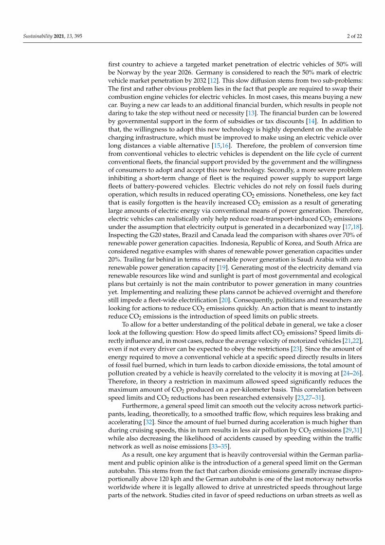
While the goal of minimizing CO2 emission is generally accepted as beneficial, discus-sions on the dimensions of restrictions necessary and acceptable to achieve these savingscontinue. To better compare the proportions of restrictions necessary for achievable CO2savings, the parallel coordinate plot in Figure 8 is used.

A completely parallel line in Figure 8 equates to a directly proportional relationbetween two parameters. An example for this is the left-hand side for a speed limit of90 km (black line). To achieve percentage-based CO2 savings of 23.16% compared to theunrestricted network state, the average speed across the network must be reduced by22.66%. In contrast to that, a steeper line in any direction (upward or downward slope)indicates a non-proportional relation between two attributes. The steeper the line, the moredisproportional the relation is. Coming back to the major example of this article, the blueline indicates a speed limit of 120 km per hour. While the left-hand side relation betweenthe average speed to be restricted and the potential savings is a positive one (an averagespeed reduction of 2.94% results in average daily CO2 savings of 7.43%), the right-handside supports claims of disproportionate incisions as 50.74% of total flow kilometers wouldrequire restrictions to achieve this 7.43% of CO2 savings. The same can be said for any ofthe other thresholds considered during this case study.

To seek a mutually acceptable compromise for both parties—supporters and oppo-nents of general speed restrictions—we took a closer look at the 120 kph restriction. In thecase of 120 kph, 50.74% of traffic flow would practically be restricted. The total CO2emissions could be reduced by 7.43%, equaling 9796.37 tons per day. Figure 9 indicates


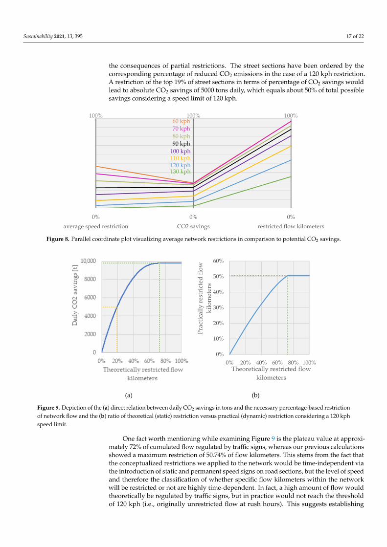
the consequences of partial restrictions. The street sections have been ordered by thecorresponding percentage of reduced CO2 emissions in the case of a 120 kph restriction.A restriction of the top 19% of street sections in terms of percentage of CO2 savings wouldlead to absolute CO2 savings of 5000 tons daily, which equals about 50% of total possiblesavings considering a speed limit of 120 kph.


(black line). To achieve percentage-based CO2 savings of 23.16% compared to the unre-stricted network state, the average speed across the network must be reduced by 22.66%. In contrast to that, a steeper line in any direction (upward or downward slope) indicates a non-proportional relation between two attributes. The steeper the line, the more dispro-portional the relation is. Coming back to the major example of this article, the blue line indicates a speed limit of 120 km per hour. While the left-hand side relation between the average speed to be restricted and the potential savings is a positive one (an average speed reduction of 2.94% results in average daily CO2 savings of 7.43%), the right-hand side supports claims of disproportionate incisions as 50.74% of total flow kilometers would require restrictions to achieve this 7.43% of CO2 savings. The same can be said for any of the other thresholds considered during this case study.

Figure 8. Parallel coordinate plot visualizing average network restrictions in comparison to potential CO2 savings.

To seek a mutually acceptable compromise for both parties—supporters and oppo-nents of general speed restrictions—we took a closer look at the 120 kph restriction. In the case of 120 kph, 50.74% of traffic flow would practically be restricted. The total CO2 emis-sions could be reduced by 7.43%, equaling 9796.37 tons per day. Figure 9 indicates the consequences of partial restrictions. The street sections have been ordered by the corre-sponding percentage of reduced CO2 emissions in the case of a 120 kph restriction. A re-striction of the top 19% of street sections in terms of percentage of CO2 savings would lead to absolute CO2 savings of 5000 tons daily, which equals about 50% of total possible sav-ings considering a speed limit of 120 kph.

60 kph70 kph80 kph90 kph

100 kph110 kph120 kph130 kph

100% 100% 100%

0% 0% 0%average speed restriction CO2 savings restricted flow kilometers

Figure 8. Parallel coordinate plot visualizing average network restrictions in comparison to potential CO2 savings.


(a) (b)

Figure 9. Depiction of the (a) direct relation between daily CO2 savings in tons and the necessary percentage-based re-striction of network flow and the (b) ratio of theoretical (static) restriction versus practical (dynamic) restriction consider-ing a 120 kph speed limit.

One fact worth mentioning while examining Figure 9 is the plateau value at approx-imately 72% of cumulated flow regulated by traffic signs, whereas our previous calcula-tions showed a maximum restriction of 50.74% of flow kilometers. This stems from the fact that the conceptualized restrictions we applied to the network would be time-inde-pendent via the introduction of static and permanent speed signs on road sections, but the level of speed and therefore the classification of whether specific flow kilometers within the network will be restricted or not are highly time-dependent. In fact, a high amount of flow would theoretically be regulated by traffic signs, but in practice would not reach the threshold of 120 kph (i.e., originally unrestricted flow at rush hours). This suggests estab-lishing dynamic traffic signs to adjust speed limits throughout different times of the day, based on actual traffic volume at specified time t. Therefore, the x-axis of Figure 9 indicates the flow that is driven on edges with potential speed signs, but its practical restriction depends on the daytime-specific actual driving speeds. As a result, the amount of flow kilometers that are theoretically restricted is higher than the amount of flow kilometers that are practically restricted. This is worth mentioning since speed limit opponents will argue based on a 72% restriction extracted from Figure 9, which in fact distorts the pro-portion of restricted flow kilometers and ignores dynamic real-world conditions. A more in-depth analysis and discussion on the topic of dynamic traffic regulation can be found in the upcoming section.

Figure 10 depicts the result in terms of absolute CO2 savings per network edge (with an average edge length of 1.8 km) throughout the German motorway network according to our network analysis. Unsurprisingly, the highest savings are to be found on motorway edges in between large cities. As proximity to city centers increases, only marginal sav-ings, if any, exist, which is to be expected since most of the traffic converges at these net-work intersections before it splits into different directions. Therefore, these highly used parts of the network predominately suffer from traffic jams, decreasing the historically averaged travel speed. Due to this decrease in average travel speed, most motorways lo-cated in close proximity to major cities are not affected by a speed limit since their default travel speed is already below the maximum speed allowed via the introduction of a speed threshold, resulting in no noteworthy CO2 savings on these network edges.

0%

10%

20%

30%

40%

50%

60%

0% 20% 40% 60% 80% 100%

Prac

tical

ly re

stri

cted

flow

ki

lom

eter

s

Theoretically restricted flow kilometers

Figure 9. Depiction of the (a) direct relation between daily CO2 savings in tons and the necessary percentage-based restrictionof network flow and the (b) ratio of theoretical (static) restriction versus practical (dynamic) restriction considering a 120 kphspeed limit.

One fact worth mentioning while examining Figure 9 is the plateau value at approxi-mately 72% of cumulated flow regulated by traffic signs, whereas our previous calculationsshowed a maximum restriction of 50.74% of flow kilometers. This stems from the fact thatthe conceptualized restrictions we applied to the network would be time-independent viathe introduction of static and permanent speed signs on road sections, but the level of speedand therefore the classification of whether specific flow kilometers within the networkwill be restricted or not are highly time-dependent. In fact, a high amount of flow wouldtheoretically be regulated by traffic signs, but in practice would not reach the thresholdof 120 kph (i.e., originally unrestricted flow at rush hours). This suggests establishing


dynamic traffic signs to adjust speed limits throughout different times of the day, based onactual traffic volume at specified time t. Therefore, the x-axis of Figure 9 indicates the flowthat is driven on edges with potential speed signs, but its practical restriction depends onthe daytime-specific actual driving speeds. As a result, the amount of flow kilometers thatare theoretically restricted is higher than the amount of flow kilometers that are practicallyrestricted. This is worth mentioning since speed limit opponents will argue based on a72% restriction extracted from Figure 9, which in fact distorts the proportion of restrictedflow kilometers and ignores dynamic real-world conditions. A more in-depth analysis anddiscussion on the topic of dynamic traffic regulation can be found in the upcoming section.

Figure 10 depicts the result in terms of absolute CO2 savings per network edge (withan average edge length of 1.8 km) throughout the German motorway network according toour network analysis. Unsurprisingly, the highest savings are to be found on motorwayedges in between large cities. As proximity to city centers increases, only marginal savings,if any, exist, which is to be expected since most of the traffic converges at these networkintersections before it splits into different directions. Therefore, these highly used parts ofthe network predominately suffer from traffic jams, decreasing the historically averagedtravel speed. Due to this decrease in average travel speed, most motorways located in closeproximity to major cities are not affected by a speed limit since their default travel speedis already below the maximum speed allowed via the introduction of a speed threshold,resulting in no noteworthy CO2 savings on these network edges.


Figure 10. Network edges colored by the amount of daily CO2 savings per edge resulting from a general speed limit of 120 kph. Brighter areas correspond to higher savings.

5. Discussion Our results verify the assumption that a general speed limit throughout the German

motorway network can help reduce the annual amount of CO2 emission by reducing av-erage travel speeds. The range of achievable savings calculated using our proposed meth-odology is in line with previous governmental studies by the German Environment Agency as well as the body of literature on this topic [24,28,30,36]

The methodology presented in this paper delivers a coherent guide on how to pro-grammatically leverage official governmental data, historical traffic information as well as open-data platforms to improve on many of the shortcomings of previous studies, mainly on the issue of non-published data sets as well as the lack of transparency and reproducibility caused by it.

As discussed in Section 4, it is not necessary to apply speed limits to the whole net-work. Instead of this, we suggest the usage of so-called Variable Speed Limits (VSL). In addition to reducing the obstacle of perceived justification, VSL contribute significant fur-ther side effects, mainly flow optimization, reduced travel times, a decrease in traffic shock waves as well as an increase in road safety in general [43–50].

Unfortunately, motorists generally do not adhere to speed limits [51]. Because of that, VSL still require enforcement to realize many of their implied benefits [52–54], which re-sults in high upfront and maintenance costs. It is therefore necessary to precisely evaluate the benefits resulting from these investments. In our case, Sections 3 and 4 focused on environmental benefits in terms of CO2 emission savings. The calculated savings of 3.6 million tons annually (by implementing a speed limit of 120 kph) would require 50.74%

Figure 10. Network edges colored by the amount of daily CO2 savings per edge resulting from ageneral speed limit of 120 kph. Brighter areas correspond to higher savings.


5. Discussion

Our results verify the assumption that a general speed limit throughout the Germanmotorway network can help reduce the annual amount of CO2 emission by reducingaverage travel speeds. The range of achievable savings calculated using our proposedmethodology is in line with previous governmental studies by the German EnvironmentAgency as well as the body of literature on this topic [24,28,30,36].

The methodology presented in this paper delivers a coherent guide on how to pro-grammatically leverage official governmental data, historical traffic information as wellas open-data platforms to improve on many of the shortcomings of previous studies,mainly on the issue of non-published data sets as well as the lack of transparency andreproducibility caused by it.

As discussed in Section 4, it is not necessary to apply speed limits to the whole network.Instead of this, we suggest the usage of so-called Variable Speed Limits (VSL). In additionto reducing the obstacle of perceived justification, VSL contribute significant further sideeffects, mainly flow optimization, reduced travel times, a decrease in traffic shock waves aswell as an increase in road safety in general [43–50].

Unfortunately, motorists generally do not adhere to speed limits [51]. Because of that,VSL still require enforcement to realize many of their implied benefits [52–54], which resultsin high upfront and maintenance costs. It is therefore necessary to precisely evaluatethe benefits resulting from these investments. In our case, Sections 3 and 4 focused onenvironmental benefits in terms of CO2 emission savings. The calculated savings of3.6 million tons annually (by implementing a speed limit of 120 kph) would require 50.74%of daily flow kilometers to be restricted throughout the network. However, this estimationresides on the lower end of the spectrum since it currently neglects the positive impactsof VSL previously described. Due to this, a wide-scale implementation of Variable SpeedLimits could lead to reduced road occupancy, resulting in a smoothed traffic flow, whichtransfers to better driving patterns that require less acceleration and braking throughout ajourney, decreasing the fuel consumption of any given vehicle, which directly correlates tofewer fossil fuels burned and less CO2 emitted throughout the network.

Unfortunately, the proposed introduction of VSL into the network highlights a majorlimitation of our methodology, since these effects cannot currently be determined becausewe adhered to simplifications and assumptions provided by the GEA for the sake ofcomparability. Due to this, future research might focus on improving on these assumptionsand supplementing the network via more specific and scientifically verifiable calculations.Some key points to be approved upon can therefore be summarized as follows:

We adopted the average-based CO2 emission functions derived by the GEA. Sincedata on how the underlying driving cycles have been calculated are non-public, we suggestbuilding transparent CO2 emission functions. To achieve this, vehicle registration datacan be analyzed to extract the distribution of different vehicle types moving on Germanmotorways. In addition to that, open access frameworks like COPERT could be utilizedto differentiate CO2 emission curves by vehicle and fuel type [55]. The biggest issue thatneeds addressing is the fact that CO2 emission functions often have a limited definitionrange. COPERT functions are currently only defined up to velocities of 130 kph. Therefore,one crucial part is finding or developing emission functions that adhere to the followingtwo requirements: (1) they should be detailed enough to differentiate between vehicleand fuel types, and (2) must be robust at higher speeds, which are driven on legallyunrestricted motorways.

Additionally, the applicability and reliability of the traffic distribution functions pro-vided by the GEA depicted in Figure 6 require further validation. Since the introductionof a general speed limit might significantly impact the driving patterns throughout thenetwork, leading to increased travel times and longer lengths of stay within the network,future studies could focus on a simulation-based approach to validate the assumed distri-bution functions and their impact on network-wide CO2 emission savings. Microscopictraffic simulation would also allow for the inclusion of VSL-based calculations [56–58],


drastically improving on the applicability of our methodology to practical debates andpotentially offsetting concerns on the topic of negative changes in driving patterns.

6. Conclusions

The contribution of this paper is a methodology to allow for transparent data analysisin road networks by enriching OpenStreetMap (OSM) data with publicly available trafficinformation on a dynamic scale.

We apply our methodology to contribute to the discussion of possible CO2 emissionsavings via the introduction of a speed limit to the German motorway network by compar-ing our programmatical results to the official study by the German Environment Agencypublished in 2020. The comparison reveals that while the key facts and estimations in termsof network infrastructure as presented by the GEA hold true, major differences betweenthe theoretical assumptions of network performance in terms of possible travel speeds andpractical data gathered by navigation service providers can be identified.

We have quantified and shown that the introduction of a flat-rate speed limit of 120 kmper hour would result in a theoretical restriction of about 70% of total flow kilometers acrossthe German motorway network, saving 3,575,675.95 tons of annual CO2 emissions withinthe transport sector. More importantly, we quantify that nearly 100% of these savings couldalready be realized by restricting only 50.74% of all network sections dynamically through-out the day due to significant variations in time-dependent road utilization. Additionalcalculations for speed limits from 60 kph to 130 kph were provided as a means of sensitivityanalysis to our findings.

Since we adopted multiple simplifying assumptions provided by the GEA for sake ofcomparability, future research might focus on speed distribution patterns in the contextof 100 and 130 kph as well as on validating the presented driving cycles to calculate thespeed-induced CO2 emissions. In addition to that, the influence of Variable Speed Limitson traffic flow smoothness and its consequences, such as the level of CO2 emissions andthe probability of accidents, are currently not included and should be analyzed in detail.

Author Contributions: Conceptualization, J.K. and M.B.; methodology, J.K. and M.B.; software, J.K.and M.B.; validation, J.K. and M.B.; writing—original draft preparation, J.K.; writing—review andediting, M.B.; visualization, M.B. and J.K.; project administration, J.K.; supervision, F.K. All authorshave read and agreed to the published version of the manuscript.

Funding: This research received no external funding.

Data Availability Statement: Data available in a publicly accessible repository.

Conflicts of Interest: The authors declare no conflict of interest.

References1. Kuramochi, T.; Roelfsema, M.; Hsu, A.; Lui, S.; Weinfurter, A.; Chan, S.; Hale, T.; Clapper, A.; Chang, A.; Höhne, N. Beyond

national climate action: The impact of region, city, and business commitments on global greenhouse gas emissions. Clim. Policy2020, 20, 275–291. [CrossRef]

2. Manne, A.; Richels, R. The Greenhouse Debate: Econonmic Efficiency, Burden Sharing and Hedging Strategies. Energy J. 1995, 16.[CrossRef]

3. Woensel, T.; Creten, R.; Vandaele, N. Managing the environmental externalities of traffic logistics: The issue of emissions. Prod.Oper. Manag. 2001, 10, 207–223. [CrossRef]

4. Kellner, F. Exploring the impact of traffic congestion on CO2 emissions in freight distribution networks. Logist. Res. 2016, 9.[CrossRef]

5. Durbin, T.D.; Johnson, K.; Miller, J.W.; Maldonado, H.; Chernich, D. Emissions from heavy-duty vehicles under actual on-roaddriving conditions. Atmos. Environ. 2008, 42, 4812–4821. [CrossRef]

6. Santos, G. Road transport and CO2 emissions: What are the challenges? Transp. Policy 2017, 59, 71–74. [CrossRef]7. Liang, Y.; Niu, D.; Wang, H.; Li, Y. Factors Affecting Transportation Sector CO2 Emissions Growth in China: An LMDI

Decomposition Analysis. Sustainability 2017, 9, 1730. [CrossRef]8. Klumpp, M. To Green or Not to Green: A Political, Economic and Social Analysis for the Past Failure of Green Logistics.

Sustainability 2016, 8, 441. [CrossRef]

http://doi.org/10.1080/14693062.2020.1740150

http://doi.org/10.5547/ISSN0195-6574-EJ-Vol16-No4-1

http://doi.org/10.1111/j.1937-5956.2001.tb00079.x

http://doi.org/10.1007/s12159-016-0148-5

http://doi.org/10.1016/j.atmosenv.2008.02.006

http://doi.org/10.1016/j.tranpol.2017.06.007

http://doi.org/10.3390/su9101730

http://doi.org/10.3390/su8050441


9. Hickman, R.; Banister, D. Looking over the horizon: Transport and reduced CO2 emissions in the UK by 2030. Transp. Policy 2007,14, 377–387. [CrossRef]

10. Haas, T.; Sander, H. Decarbonizing Transport in the European Union: Emission Performance Standards and the Perspectives for aEuropean Green Deal. Sustainability 2020, 12, 8381. [CrossRef]

11. Lajunen, A.; Kivekäs, K.; Vepsäläinen, J.; Tammi, K. Influence of Increasing Electrification of Passenger Vehicle Fleet on CarbonDioxide Emissions in Finland. Sustainability 2020, 12, 5032. [CrossRef]

12. Rietmann, N.; Hügler, B.; Lieven, T. Forecasting the trajectory of electric vehicle sales and the consequences for worldwide CO2emissions. J. Clean. Prod. 2020, 261, 121038. [CrossRef]

13. Bienias, K.; Kowalska-Pyzalska, A.; Ramsey, D. What do people think about electric vehicles? An initial study of the opinions ofcar purchasers in Poland. Energy Rep. 2020, 6, 267–273. [CrossRef]

14. Kapustin, N.O.; Grushevenko, D.A. Long-term electric vehicles outlook and their potential impact on electric grid. Energy Policy2020, 137, 111103. [CrossRef]

15. Funke, S.Á.; Sprei, F.; Gnann, T.; Plötz, P. How much charging infrastructure do electric vehicles need? A review of the evidenceand international comparison. Transp. Res. Part D Transp. Environ. 2019, 77, 224–242. [CrossRef]

16. Greene, D.L.; Kontou, E.; Borlaug, B.; Brooker, A.; Muratori, M. Public charging infrastructure for plug-in electric vehicles: What isit worth? Transp. Res. Part D Transp. Environ. 2020, 78, 102182. [CrossRef]

17. Fridstrøm, L. Who will bell the cat? On the environmental and sustainability risks of electric vehicles: A comment. Transp. Res.Part A Policy Pract. 2020, 135, 354–357. [CrossRef]

18. Kawamoto, R.; Mochizuki, H.; Moriguchi, Y.; Nakano, T.; Motohashi, M.; Sakai, Y.; Inaba, A. Estimation of CO2 Emissions ofInternal Combustion Engine Vehicle and Battery Electric Vehicle Using LCA. Sustainability 2019, 11, 2690. [CrossRef]

19. Ram, M.; Child, M.; Aghahosseini, A.; Bogdanov, D.; Lohrmann, A.; Breyer, C. A comparative analysis of electricity generationcosts from renewable, fossil fuel and nuclear sources in G20 countries for the period 2015-2030. J. Clean. Prod. 2018, 199, 687–704.[CrossRef]

20. Canals Casals, L.; Martinez-Laserna, E.; Amante García, B.; Nieto, N. Sustainability analysis of the electric vehicle use in Europefor CO2 emissions reduction. J. Clean. Prod. 2016, 127, 425–437. [CrossRef]

21. Shirazinejad, R.S.; Dissanayake, S. Speed Characteristics in Relation to Speed Limit Increase and Its Influence on Driver’s SpeedSelection Behavior. Sustainability 2020, 12, 1369. [CrossRef]

22. Yang, J.; Xu, J.; Gao, C.; Bai, G.; Xie, L.; Li, M. Modeling of the Relationship Between Speed Limit and Characteristic Speed ofExpressway Traffic Flow. Sustainability 2019, 11, 4621. [CrossRef]

23. Fergusson, M. The effect of vehicle speeds on emissions. Energy Policy 1994, 22, 103–106. [CrossRef]24. Keller, J.; Andreani-Aksoyoglu, S.; Tinguely, M.; Flemming, J.; Heldstab, J.; Keller, M.; Zbinden, R.; Prevot, A.S.H. The impact of

reducing the maximum speed limit on motorways in Switzerland to 80km h−1 on emissions and peak ozone. Environ. Model.Softw. 2008, 23, 322–332. [CrossRef]

25. Frey, H.C.; Rouphail, N.M.; Zhai, H. Speed- and Facility-Specific Emission Estimates for On-Road Light-Duty Vehicles on theBasis of Real-World Speed Profiles. Transp. Res. Rec. J. Transp. Res. Board 2006, 1987, 128–137. [CrossRef]

26. Lejri, D.; Can, A.; Schiper, N.; Leclercq, L. Accounting for traffic speed dynamics when calculating COPERT and PHEM pollutantemissions at the urban scale. Transp. Res. Part D Transp. Environ. 2018, 63, 588–603. [CrossRef]

27. Chang, C.-C.; Wang, C.-M. Evaluating the effects of speed reduce for shipping costs and CO2 emission. Transp. Res. Part D Transp.Environ. 2014, 31, 110–115. [CrossRef]

28. Int Panis, L.; Beckx, C.; Broekx, S.; de Vlieger, I.; Schrooten, L.; Degraeuwe, B.; Pelkmans, L. PM, NOx and CO2 emissionreductions from speed management policies in Europe. Transp. Policy 2011, 18, 32–37. [CrossRef]

29. Int Panis, L.; Broekx, S.; Liu, R. Modelling instantaneous traffic emission and the influence of traffic speed limits. Sci. Total Environ.2006, 371, 270–285. [CrossRef] [PubMed]

30. Keuken, M.P.; Jonkers, S.; Wilmink, I.R.; Wesseling, J. Reduced NOx and PM10 emissions on urban motorways in The Netherlandsby 80 km/h speed management. Sci. Total Environ. 2010, 408, 2517–2526. [CrossRef]

31. Madireddy, M.; de Coensel, B.; Can, A.; Degraeuwe, B.; Beusen, B.; de Vlieger, I.; Botteldooren, D. Assessment of the impactof speed limit reduction and traffic signal coordination on vehicle emissions using an integrated approach. Transp. Res. Part DTransp. Environ. 2011, 16, 504–508. [CrossRef]

32. Gao, C.; Xu, J.; Li, Q.; Yang, J. The Effect of Posted Speed Limit on the Dispersion of Traffic Flow Speed. Sustainability 2019, 11,3594. [CrossRef]

33. Kleiziene, R.; Šernas, O.; Vaitkus, A.; Simanaviciene, R. Asphalt Pavement Acoustic Performance Model. Sustainability 2019, 11,2938. [CrossRef]

34. Park, T.; Kim, M.; Jang, C.; Choung, T.; Sim, K.-A.; Seo, D.; Chang, S. The Public Health Impact of Road-Traffic Noise in aHighly-Populated City, Republic of Korea: Annoyance and Sleep Disturbance. Sustainability 2018, 10, 2947. [CrossRef]

35. Casado-Sanz, N.; Guirao, B.; Attard, M. Analysis of the Risk Factors Affecting the Severity of Traffic Accidents on SpanishCrosstown Roads: The Driver’s Perspective. Sustainability 2020, 12, 2237. [CrossRef]

36. Lange, M.; Hendzlik, M.; Schmied, M. Klimaschutz durch Tempolimit. In Wirkung Eines Generellen Tempolimits Auf Bundesautobah-nen Auf Die Treibhausgasemissionen; Umweltbundesamt: Dessau-Roßlau, Germany, 2020.


http://doi.org/10.3390/su12208381

http://doi.org/10.3390/su12125032

http://doi.org/10.1016/j.jclepro.2020.121038

http://doi.org/10.1016/j.egyr.2019.08.055

http://doi.org/10.1016/j.enpol.2019.111103

http://doi.org/10.1016/j.trd.2019.10.024

http://doi.org/10.1016/j.trd.2019.11.011

http://doi.org/10.1016/j.tra.2020.03.017

http://doi.org/10.3390/su11092690

http://doi.org/10.1016/j.jclepro.2018.07.159

http://doi.org/10.1016/j.jclepro.2016.03.120

http://doi.org/10.3390/su12041369

http://doi.org/10.3390/su11174621

http://doi.org/10.1016/0301-4215(94)90126-0

http://doi.org/10.1016/j.envsoft.2007.04.008

http://doi.org/10.1177/0361198106198700114

http://doi.org/10.1016/j.trd.2018.06.023

http://doi.org/10.1016/j.trd.2014.05.020


http://doi.org/10.1016/j.scitotenv.2006.08.017

http://www.ncbi.nlm.nih.gov/pubmed/17049967

http://doi.org/10.1016/j.scitotenv.2010.03.008

http://doi.org/10.1016/j.trd.2011.06.001

http://doi.org/10.3390/su11133594

http://doi.org/10.3390/su11102938

http://doi.org/10.3390/su10082947

http://doi.org/10.3390/su12062237


37. Löhe, U. Geschwindigkeiten auf Bundesautobahnen in den Jahren 2010 bis 2014. In Schlussbericht Zum AP-Projekt F1100.6213001;Bundesanstalt für Straßenwesen: Bergisch Gladbach, Germany, 2016.

38. Zhang, S.; Witlox, F. Analyzing the Impact of Different Transport Governance Strategies on Climate Change. Sustainability 2020,12, 200. [CrossRef]

39. Haklay, M. How Good is Volunteered Geographical Information? A Comparative Study of OpenStreetMap and Ordnance SurveyDatasets. Environ. Plann. B Plann. Des. 2010, 37, 682–703. [CrossRef]

40. Jacobs, K.T.; Mitchell, S.W. OpenStreetMap quality assessment using unsupervised machine learning methods. Trans. GIS 2020,24, 1280–1298. [CrossRef]

41. Boeing, G. OSMnx: New methods for acquiring, constructing, analyzing, and visualizing complex street networks. Comput.Environ. Urban Syst. 2017, 65, 126–139. [CrossRef]

42. DIN EN 16258: 2012. Methodology for Calculation and Declaration of Energy Consumption and GHG Emissions of Transport Services(Freight and Passengers); European Committee for Standardization: Brussels, Belgium, 2012.

43. Heydecker, B.G.; Addison, J.D. Analysis and modelling of traffic flow under variable speed limits. Transp. Res. Part C Emerg.Technol. 2011, 19, 206–217. [CrossRef]

44. Khondaker, B.; Kattan, L. Variable speed limit: An overview. Transp. Lett. 2015, 7, 264–278. [CrossRef]45. Papageorgiou, M.; Kosmatopoulos, E.; Papamichail, I. Effects of Variable Speed Limits on Motorway Traffic Flow. Transp. Res. Rec.

2008, 2047, 37–48. [CrossRef]46. Bertini, R.L.; Boice, S.; Bogenberger, K. Dynamics of Variable Speed Limit System Surrounding Bottleneck on German Autobahn.

Transp. Res. Rec. 2006, 1978, 149–159. [CrossRef]47. Hegyi, A.; DeSchutter, B.; Hellendoorn, J. Optimal Coordination of Variable Speed Limits to Suppress Shock Waves. IEEE Trans.

Intell. Transport. Syst. 2005, 6, 102–112. [CrossRef]48. Abdel-Aty, M.; Dilmore, J.; Dhindsa, A. Evaluation of variable speed limits for real-time freeway safety improvement. Accid. Anal.

Prev. 2006, 38, 335–345. [CrossRef] [PubMed]49. Islam, M.T.; Hadiuzzaman, M.; Fang, J.; Qiu, T.Z.; El-Basyouny, K. Assessing Mobility and Safety Impacts of a Variable Speed

Limit Control Strategy. Transp. Res. Rec. 2013, 2364, 1–11. [CrossRef]50. Lee, C.; Hellinga, B.; Saccomanno, F. Evaluation of variable speed limits to improve traffic safety. Transp. Res. Part C Emerg.

Technol. 2006, 14, 213–228. [CrossRef]51. Wilmot, C.G.; Khanal, M. Effect of Speed limits on speed and safety: A review. Transp. Rev. 1999, 19, 315–329. [CrossRef]52. Hirst, W.M.; Mountain, L.J.; Maher, M.J. Are speed enforcement cameras more effective than other speed management measures?

An evaluation of the relationship between speed and accident reductions. Accid. Anal. Prev. 2005, 37, 731–741. [CrossRef]53. Montella, A.; Imbriani, L.L.; Marzano, V.; Mauriello, F. Effects on speed and safety of point-to-point speed enforcement systems:

Evaluation on the urban motorway A56 Tangenziale di Napoli. Accid. Anal. Prev. 2015, 75, 164–178. [CrossRef]54. Soole, D.W.; Watson, B.C.; Fleiter, J.J. Effects of average speed enforcement on speed compliance and crashes: A review of the

literature. Accid. Anal. Prev. 2013, 54, 46–56. [CrossRef] [PubMed]55. O’Driscoll, R.; ApSimon, H.M.; Oxley, T.; Molden, N.; Stettler, M.E.J.; Thiyagarajah, A. A Portable Emissions Measurement System

(PEMS) study of NOx and primary NO2 emissions from Euro 6 diesel passenger cars and comparison with COPERT emissionfactors. Atmos. Environ. 2016, 145, 81–91. [CrossRef]

56. Arnaout, G.M.; Arnaout, J.-P. Exploring the effects of cooperative adaptive cruise control on highway traffic flow using microscopictraffic simulation. Transp. Plan. Technol. 2014, 37, 186–199. [CrossRef]

57. Barcel, J.; Codina, E.; Casas, J.; Ferrer, J.L.; Garca, D. Microscopic traffic simulation: A tool for the design, analysis and evaluationof intelligent transport systems. J. Intell. Robot Syst. 2005, 41, 173–203. [CrossRef]

58. So, J.; Motamedidehkordi, N.; Wu, Y.; Busch, F.; Choi, K. Estimating emissions based on the integration of microscopic trafficsimulation and vehicle dynamics model. Int. J. Sustain. Transp. 2018, 12, 286–298. [CrossRef]

http://doi.org/10.3390/su12010200

http://doi.org/10.1068/b35097

http://doi.org/10.1111/tgis.12680

http://doi.org/10.1016/j.compenvurbsys.2017.05.004

http://doi.org/10.1016/j.trc.2010.05.008

http://doi.org/10.1179/1942787514Y.0000000053

http://doi.org/10.3141/2047-05

http://doi.org/10.1177/0361198106197800119

http://doi.org/10.1109/TITS.2004.842408

http://doi.org/10.1016/j.aap.2005.10.010


http://doi.org/10.3141/2364-01

http://doi.org/10.1016/j.trc.2006.06.002

http://doi.org/10.1080/014416499295420

http://doi.org/10.1016/j.aap.2005.03.014

http://doi.org/10.1016/j.aap.2014.11.022

http://doi.org/10.1016/j.aap.2013.01.018


http://doi.org/10.1016/j.atmosenv.2016.09.021

http://doi.org/10.1080/03081060.2013.870791

http://doi.org/10.1007/s10846-005-3808-2

http://doi.org/10.1080/15568318.2017.1363328

speed limit induced co2 reduction on motorways: enhancing

Documents