speed limit and asymmetric inflation effects … · oecd economic studies no. 24, i995/1 speed...

OECD Economic Studies No. 24, I995/1

SPEED LIMIT AND ASYMMETRIC INFLATION EFFECTS FROM THE OUTPUT GAP IN THE MAJOR SEVEN ECONOMIES

Dave Turner

TABLE OF CONTENTS

Introduaion ....................................................... 58 Estimation of reduced form equations to explain inflation . . . . . . . . . . . . . . . . . . . 60 Speed limit effects in the linear model . . . . . . . . . . . . . . . . . . . . . . . . . . . . . . . . . . 61

Asymmetric effects from positive and negative output gaps on inflation . '. . . . . . . 63 Allowing for possible mismeasurement of the gap . . . . . . . . . . . . . . . . . . . . . . . 64 An illustrative example . . . . . . . . . . . . . . . . . . . . . . . . . . . . . . . . . . . . . . . . . . . . 66

Summary and policy implications. . . . . . . . . . . . . . . . . . . . . . . . . . . . . . . . . . . . . . . 69 Annex 1. Algebraic proofs.. . . . . . . . . . . . . . . . . . . . . . . . . . . . . . . . . . . . . . . . . . 73 Annex 2. Estimation results . . . . . . . . . . . . . . . . . . . . . . . . . . . . . . . . . . . . . . . . . . 77 Bibliography ....................................................... 87

The author is currently working in Country Studies I Division of the OECD Economics Depart- ment. He would like to thank Jergen Elmeskov and David Grubb for helpful comments and suggestions and Diane Tufek and Frangoise Correia for the technical preparation of the paper.

571

INTRODUCTION

((Fast growing economies, like champagne parties, have a habit of spinning out of control, unleashing inflation ... Typically, policy makers wait too late to spoil the fun, and they thereby increase the likelihood that growth will turn abruptly to recession. ))

The Economist magazine (ID December 1994)

((Employment growth was rapid and the OED-wide unemployment rate was brought down to 6% per cent in 1990, ... OECD inflation fell to a 25-year low of less than 3 per cent in 1986. This was a missed opportunity to lock in low inflation given the acknowledged cost of disinflation. 2

OECD ( I 994a)

Economic commentators and policy-makers often emphasise that timing is important in macroeconomic policy-making and that mistakes can be costly, as illustrated by the quotations above. Such views contrast with the predictions of much empirical modelling of the inflation process where linear, or near linear, relationships between inflation and output predominate. A linear relationship implies that an increase in inflation resulting from excessive output can be reversed by following policies which ensure an equivalent reduction in output.] Thus, no permanent penalty, in terms of higher inflation or lost output, is ultimately paid for errors in macroeconomic policy-making or, as De Long and Summers (1988) put it, ((policies can do no first order good or harm on the output side without perma- nently raising or lowering the inflation rate,). This paper considers the empirical evidence of some alternatives to the simple linear relationship between output and inflation which imply a more important role for macroeconomic policy.

A common approach to empirical modelling of inflation involves estimates of the a output gap )>, namely the difference between (( potential )> output and actual output.2 This approach assumes that there exists some identifiable path of potential output, such that i f output rises above it, then there will be an increase in inflation (possibly with some lag) and conversely if output falls below potential output then there will be a fall in inflation. For example, commenting on the relationship between inflation and the output gap for the major seven economies, similar to that shown in Figure I , the OECD (1991) argued that :

Speed limit and asymmetric inflation effects from the output gap in the major seven economies

Figure I. Inflation and the output gap for the major seven OECD economies

Per cent Per cent 14 14

12 12

10 10

a a

6 6

4

2

4

2

0 0

-2 -2

4 -4

1960 62 64 66 68 70 72 74 76 78 ao a2 a4 a6 aa 90 92

Source: OECD.

((There appears to be a relatively close link over time between the size of the output gap and the change in average inflation for the aggregate of the major OECD economies. As a rule of thumb, a negative output gap of 1 per cent has been associated with a reduction in inflation, as measured by the GDP deflator, of slightly more than percentage point each year in the major countries taken together. Large divergences from this pattern have not occurred since the first oil shock.)> The concept of potential output is thus similar to that of the non-accelerating

wagedinflation rate of unemployment (NAWRU or NAIRU) for the labour market. Indeed, Torres and Martin (1990) derive series for potential output by substituting a measure of potential employment which is consistent with the NAWRU into an estimated production function for the main OECD economies. This work has been updated by Giorno et al. in an article in this issue. Other less theoretically based approaches to deriving a measure of potential output involve simply smoothing actual output, for example using moving average method or a Hodrick-Prescott filter.3

In addition to evaluating the size of the output gap it is necessary to have some view of the nature of the relationship between the output gap and inflation in order to assess inflationary risks. This paper focuses on two departures from the simple linear relationship whereby inflationary pressures are judged in direct proportion to the size and sjgn of the output gap.4 The first is whether there is empirical evidence of a ((speed limit )) effect such that i f the gap between actual and potential output is closed quickly, then inflation can increase, even though output never rises above .i??

OECD - ronornic Studies No. 24, 199511

potential. Such <(speed limit, effects can be represented as a special case of a linear relationship between the output gap and inflation. The second issue concerns a complete departure from the linear model, namely whether there is evidence of an asymmetry in the inflationary effect of output gaps so that the inflationary effect of output being above potential is greater than the deflationary effect of output being below potential.

The remainder of the paper is organised as follows. In the first section the estimation of reduced form equations explaining inflation for each of the major seven OECD economies is described. The issue of speed limits is examined by reference to these equations in the section on speed limit effects in the linear model. In the third section variants of the equations are estimated in which allow- ance is made for possible asymmetric effects from negative and positive output gaps. Finally, the main results from the paper are summarised and the implications for policy are discussed in the final section. Various algebraic proofs are in given in Annex 1 and details of the estimation results are given in Annex 2.

ESTIMATION OF REDUCED FORM EQUATIONS TO EXPLAlN INFLATION For each of the major seven OECD economies a reduced form equation for the

change in inflation is estimated as a dynamic function of the output gap, using annual data starting in the early 1960s. Inflation is measured in terms of the non-oil GDP deflator at factor cost, in order to exclude the direct effect of oil shocks on those economies [the United States, Canada and the United Kingdom) with significant oil production sectors as well as to exclude the effect of changes in net indirect taxes. The output gap is defined as the percentage deviation of real GDP from potential, the latter being proxied by using a Hodrick-Prescott filter on (the logarithm of) actual GDP (see Annex 2 for further detail^).^ The change in inflation is regressed on contemporaneous and lagged output gap variables as well as other variables designed to capture the effect of supply shocks.

The variables included to capture the effect of supply shocks can mostly be described as various measures of the <wedge)+ or components of it : tax rates, import prices (weighted according to the weight of imports in total expenditure), total domestic demand prices and consumer prices. The price variables enter the equation either in terms of relative inflation rates (e.g. consumer price less output price inflation) or relative price levels (e.g. the level of consumer prices relative to the level of output prices), according to which is preferred statistically. The latter functional form implies stronger real wage resistance, since inflation responds not only to current and recent lagged differences in relative inflation rates, but also to all past differences reflected in relative price levels. In addition, a number of country specific dummy variables are included : in the equation for Canada to capture the operation of the Anti-Inflation Board in 1976 and 1977; in the equation for France to capture the effect of the general strike in 1968; and in the equation For the United Kingdom in 1976 and 1977 to capture the effect of incomes p ~ l i c y . ~ The equations also include a constant which has no theoretical role [and is ignored in empirical &


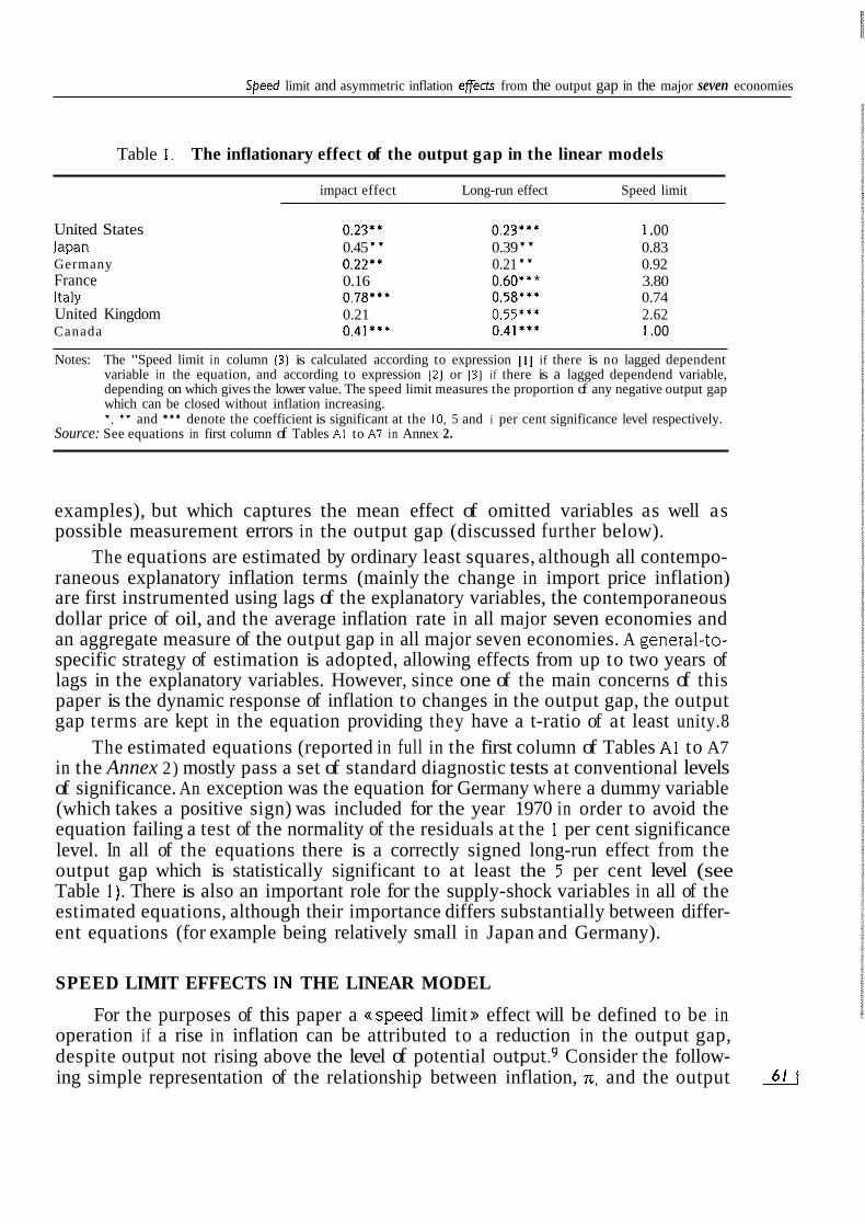
Table 1 . The inflationary effect of the output gap in the linear models

impact effect Long-run effect Speed limit

United States 0.23** 0.23"' 1 .oo lapan 0.45" 0.39" 0.83 Germany 0.22'' 0.21" 0.92 France 0.16 0.60** * 3.80 Italy 0.78''' 0.58*** 0.74 United Kingdom 0.21 0.55*** 2.62 Canada 0.41*** 0.41*** I .oo Notes: The "Speed limit in column (3) is calculated according to expression I l l if there is no lagged dependent

variable in the equation, and according to expression 121 or 131 i f there is a lagged dependend variable, depending on which gives the lower value. The speed limit measures the proportion of any negative output gap which can be closed without inflation increasing. *. * * and * * * denote the coefficient is significant at the 10. 5 and i per cent significance level respectively.

Source: See equations in first column of Tables Al to A 1 in Annex 2.

examples), but which captures the mean effect of omitted variables as well as possible measurement errors in the output gap (discussed further below).

The equations are estimated by ordinary least squares, although all contemporaneous explanatory inflation terms (mainly the change in import price inflation) are first instrumented using lags of the explanatory variables, the contemporaneous dollar price of oil, and the average inflation rate in all major seven economies and an aggregate measure of the output gap in all major seven economies. A general-to- specific strategy of estimation is adopted, allowing effects from up to two years of lags in the explanatory variables. However, since one of the main concerns of this paper is the dynamic response of inflation to changes in the output gap, the output gap terms are kept in the equation providing they have a t-ratio of at least unity.8

The estimated equations (reported in full in the first column of Tables A1 to A7 in the Annex 2) mostly pass a set of standard diagnostic tests at conventional levels of significance. An exception was the equation for Germany where a dummy variable (which takes a positive sign) was included for the year 1970 in order to avoid the equation failing a test of the normality of the residuals at the 1 per cent significance level. In all of the equations there is a correctly signed long-run effect from the output gap which is statistically significant to at least the 5 per cent level (see Table 1 ) . There is also an important role for the supply-shock variables in all of the estimated equations, although their importance differs substantially between different equations (for example being relatively small in Japan and Germany).

SPEED LIMIT EFFECTS IN THE LINEAR MODEL

For the purposes of this paper a <(speed limit )) effect will be defined to be in operation if a rise in inflation can be attributed to a reduction in the output gap, despite output not rising above the level of potential o ~ t p u t . ~ Consider the following simple representation of the relationship between inflation, n. and the output 4

OECD Economic Studies No. 24, I99511

gap, GAP (which encompasses the linear models estimated for each of the major seven countries) :

111 where A is the first difference operator, subscripts denote lags and Po and (Po + 0,) are both positive. Consider first the simple case where there is no inertia to changes in inflation so that a, = a, = 0. Now suppose that in period 1 output is below potential, GAP, = GAP* c 0, and that in period 2 the gap is closed and output equals potential, i.e. GAP, = 0, then for inflation to rise (An, > 0) PI must be negative, so that the impact effect of the gap on inflation must be greater than t h e total effect in the period following the impact. If this condition does hold, then the extent of the speed limit is determined in terms of the proportion,@ of the output gap which can be closed without increasing inflation. This speed limit can be calculated as the ratio of the impact plus lagged effect of the output gap on inflation to the impact effect of the output gap Ifor proof of expressions 121, 131 and 141 for the speed limit see Annex 11. thus :

121 If there is inertia to changes in inflation, so that a, or a2 are not zero, then the

calculation of the speed limit effect is more complicated because it involves the history of past inflation. Two extreme cases are therefore considered, although these are by no means exhaustive of all possibilities. Firstly, it is assumed that there has been a zero output gap for several periods prior to the downturn in period 1 so that inflation is stable and in period 1 inflation falls at the rate predicted by equation 111, so that An, = Po GAP*. In this case the speed limit is calculated as :

131 Alternatively, assume that the economy has been running a negative output

gap, GAP', for a number of periods prior to period I so that inflation is falling (both in period 1 and prior to it) at a steady state rate of (Po + P,)GAP'/( 1 - a, - a2), a s predicted by equation 11 1. In this second case the speed limit is given as the ratio of the long-run effect to the impact effect of the output gap :

An = Po GAP + 0 , GAP-, + a, An-, + a, An-, + .. supply-side shocks,

0 = (Po + P,)/PO

8 = (pea, + so + P, ) /P~

e = i(p0 + P,)N - a, - ~ , ) I / P ~ 141 In Table 1 the speed limits for each of the major seven economies are calcu-

lated from the estimated linear equations. In those cases where there are lagged inflation terms in the estimated equation, expression 131 or 141 is chosen to evaluate the speed limit effect according to whichever gives the the most binding speed limit effect (i.e. the lowest value of 8).

For three of the seven countries a speed limit effect does operate, so that the value of e is less than one, implying that only a proportion of any negative output gap can be closed without inflation rising. However, even in these cases the speed limit effect is not particularly tight with Italy, lapan and Germany being able to close up to 74, 83 and 92 per cent of any negative output gap respectively, without inflation risinglo. For both the United States and Canada €I is close to one, so that the impact and long-run effect of the output gap on inflation are similar, implying W

Speed limit and asymmetric inpotion effects from the output gap in the major seven economies

that inflation will respond quickly to the current gap, but that there is no speed limit effect. There is no evidence of a speed limit effect for either France or the United Kingdom, with the estimated value of 8 much greater than one.

Moreover, the importance of the speed limit effect should not be over- emphasised. In particular, the change in inflation over the course of an entire recession and recovery phase will be completely independent of the existence or scale of any speed limit effect. More formally, the sacrifice ratio, the ratio of the cumulative loss in output to the reduction in inflation, is given by the reciprocal of the the long-run effect of the output gap (i.e. (Po + &)/ ( I - a, - a?) in terms of equation 11 I ) and is independent of the speed limit effect (for proof see Annex I ) .

ASYMMETRIC EFFECTS FROM POSITIVE AND NEGATIVE OUTPUT GAPS ON INFLATION

In this section the empirical evidence as to whether the inflationary effect of output being above potential is greater than the deflationary effect of output being below potential is examined. Such an asymmetry has a long tradition in macroeconomic theory, corresponding to the Keynesian idea that the aggregate supply curve is kinked, being roughly horizontal up to some notion of full employment or potential output, beyond which it becomes very steep and even vertical. Recent work by Ball and Mankiw (1994) provides some microeconomic basis for asymmetrical inflation effects. They describe a menu-cost model of pricing behaviour where positive shocks to firm’s desired prices generate faster adjustment than negative shocks, since in the latter case the adjustment of relative prices can be at least partially achieved by the presence of trend inflation.”

Asymmetric or non-linear effects from demand on inflation do not, however, feature strongly in most empirical macroeconometric models.I2 An exception is the Bank of Canada model, following the work by Laxton et a/. (1993b). which found evidence of such asymmetry when estimating a reduced form inflation equation on annual data for Canada, see Coletti et a/. (1994). The findings of Laxton et a/. ( l993b) suggest that the inflationary effects of a positive output gap are more than five times as great as the deflationary effect from a similar negative output gap and that, in addition, inflation responds more quickly to a positive gap. Recent work by Laxton et a/. (1994). discussed further below, also finds evidence of such asymmetric non-linearities using a pooled estimation technique for the major seven economies. The restrictions necessary to transform their preferred non-linear asymmetric model of inflation to a more standard linear model are overwhelmingly rejected.I3

In the present paper, the hypothesis of asymmetric gap effects is initially investigated by allowing differences between the effects of positive and negative output gaps in the estimated equations discussed in previous sections (this is similar to the approach followed by Laxton et a/., 1993b). Positive and negative output gap terms are retained in the equation, as before, providing that they have a t-ratio of at least unity. The resulting equations (tabulated in the second column of 4

OECD Economic Studies No. 24. 199511

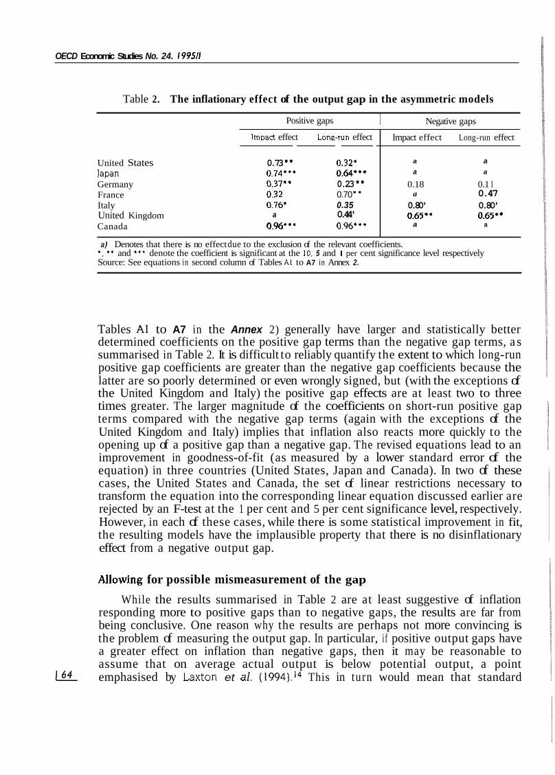
Table 2. The inflationary effect of the output gap in the asymmetric models

I Negative gaps Positive gaps

Impact effect Lona-run effect

United States Japan Germany France Italy United Kingdom Canada

~ ~ ~~ ~

0.73" 0.32' 0.74*** 0.64'" 0.37'' 0.23" 0.32 0.70" 0.76* 0.35

a 0.44' 0.96' * * 0.96**'

Impact effect Long-run effect

a a a a

0.18 0.1 I a 0.47 0.80' 0.80' 0.65.' 0.65''

a a

a) Denotes that there is no effect due to the exclusion of the relevant coefficients. *. * * and * * * denote the coefficient is significant at the 10. 5 and I per cent significance level respectively Source: See equations in second column of Tables A l to A7 in Annex 2.

Tables A1 to A7 in the Annex 2) generally have larger and statistically better determined coefficients on the positive gap terms than the negative gap terms, a s summarised in Table 2. It is difficult to reliably quantify the extent to which long-run positive gap coefficients are greater than the negative gap coefficients because the latter are so poorly determined or even wrongly signed, but (with the exceptions of the United Kingdom and Italy) the positive gap effects are at least two to three times greater. The larger magnitude of the coefficients on short-run positive gap terms compared with the negative gap terms (again with the exceptions of the United Kingdom and Italy) implies that inflation also reacts more quickly to the opening up of a positive gap than a negative gap. The revised equations lead to an improvement in goodness-of-fit (as measured by a lower standard error of the equation) in three countries (United States, Japan and Canada). In two of these cases, the United States and Canada, the set of linear restrictions necessary to transform the equation into the corresponding linear equation discussed earlier are rejected by an F-test at the 1 per cent and 5 per cent significance level, respectively. However, in each of these cases, while there is some statistical improvement in fit, the resulting models have the implausible property that there is no disinflationary effect from a negative output gap.

Mowing for possible mismeasurement of the gap

While the results summarised in Table 2 are at least suggestive of inflation responding more to positive gaps than to negative gaps, the results are far from being conclusive. One reason why the results are perhaps not more convincing is the problem of measuring the output gap. In particular, i f positive output gaps have a greater effect on inflation than negative gaps, then it may be reasonable to assume that on average actual output is below potential output, a point emphasised by Laxton et al. (1994).14 This in turn would mean that standard

Speed limit ond asymmetric inpotion effects from the output gap in the major seven economies

methods of estimating potential output (such as the Hodrick-Prescott filter adopted here), which typically produce some smoothed trend of actual output, may be systematically over-estimating potential output. Laxton eta!. (1993) present Monte- Carlo evidence which shows that i f the true data generation process does have asymmetric effects from inflation, a failure to allow for this mismeasurement strongly biases tests towards the acceptance of a linear approximations. However, given the limited span of time series data typically being worked with, it is difficult to simultaneously identify the bias in the gap as well as a non-linear relationship between the gap and inflation. In order to overcome this problem Laxton et a/. (1994) adopt a pooled estimation technique in which common parameters across the major seven OECD countries are imposed. The use of a pooled estimation approach, however, clearly relies on the assumption of similarity in the processes generating inflation across economies with widely different institutional frameworks and widely different histories of macroeconomic performance.15

An alternative approach which is adopted here is to assume a simple relationship between the mismeasurement of the output gap and the form of the non-linear relationship between inflation and the output gap. Thus i f , for example, it is assumed that a positive gap has an effect on inflation which is double the effect of a negative gap, then the output gap derived from the Hodrick-Prescott filter is adjusted by subtracting a constant to give the result that over the full sample period the sum of all negative output gaps is double the sum of all positive gaps.l6 More formally, if a constant 6, is subtracted from the Hodrick-Prescott gap measure, GAP, so that the cumulative negative output gap is c n )> times the cumulative positive gap, then the form of the gap which is included in the reduced form inflation equation is f,(GAP), where :

f,(GAP) = n (GAP - 6) if (GAP - 6) > 0 = (GAP- 6) if (GAP-6) < 0.

151

Thus 6 is calculated, dependent on n , to ensure that the weighted sum of positive and negative gap terms is zero (ie. C f,(GAP) = 0, where C denotes the sum over the entire sample period). For each country f,(GAP) is calculated for values of n of 2, 3, 4 and 5 and the value of n chosen according to which f,(GAP) gives the greatest goodness-of-fit when substituted For the linear GAP variables (which correspond to the case n = 1 ) in the estimated reduced form inflation equations.17

The results from following this estimation procedure are summarised in Table 3 with full details of the equations (for the optimal value of n ) detailed in the third column of Tables Al to A7 in the Annex 2. For five of the seven countries some improvement in goodness-of-fit (as measured by a lower standard error to the equation) is achieved relative to the linear model. The values of n which maximise the goodness-of-fit are 4 for the United States, Japan and Canada, 2 for Germany and France, whereas for both the United Kingdom and Italy the transformed gap measures do not give any improvement in goodness-of-fit over the linear model. In three of the fives cases (the United States, Canada and Japan) where there is some improvement over the linear model, the linear model is rejected at least at the 5 per 4


Table 3. Tests for alternative asymmetric models

Value of "n" Magnitude of

('I F-test versus linear Model2 for fJGAP) giving greatest to the output gap

goodness-of-fit (per cent of GDP)

United States 4 0.89 Linear model rejected at 1 per cent level lapan 4 1.1 I Linear model rejected at 5 per cent level Germany 2 0.71 Not possible to reject linear model France 2 0.47 Not possible to reject linear model Italy I - Not applicable United Kingdom I - Not applicable Canada 4 0.92 Linear model rejected at 5 per cent level

I . Greatest goodness-of-ht is iudged by lowest standard error for the equation. A value of "n" of I signifies the linear model is preferred.

2. The test is carried out by constructing a composite equation of the linear model and the asymmetric model with f,(GAP) and then conducting an F-test to see whether the linear model is a valid restriction of the composite model.

cent significance level as a restriction of the more general composite model which includes both the linear and transformed gap terms. This is, however, quite a strict test of the asymmetry. because there is a high degree of collinearity between t h e alternative measures of the output gap lie. GAP and fn(GAP)] in the composite equation, which will tend to bias against rejection of the linear model.

The magnitude of the constant adjustment, 6, to the Hodrick-Prescott measure of the gap is between 0.9 and 1 .1 per cent for the United States, Japan, and Canada, and 0.5 to 0.7 per cent for France and Germany. The magnitude of these adjust- ments can be compared with the constant adjustment of 0.6 per cent which Laxton et a/. (1994) estimate for the major seven countries using a pooled estimation technique.

The two countries, Italy and United Kingdom, where the linear model is favoured over asymmetric alternatives are also those (together with japan) where the standard error of the equation is largest. They are also the two countries where, arguably, structural reform, particularly in the labour market, has had most influ- ence in changing the processes which determine inflation. Barrel1 (1990) finds evidence of a structural break in estimated wage equations for Italy in the early 1980s. which is attributed to the gradual dismantling of wage fixing agreements under the Scala Mobile. If the reduced form inflation equation is estimated for Italy. but only using data from 1980 onwards, then an asymmetric model is preferred to

L4L linear alternatives.


An illustrative example In order to demonstrate the importance of these asymmetries, the behaviour of

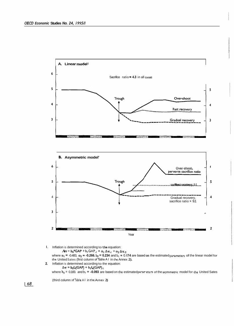
inflation in various recovery scenarios from a hypothetical recession are considered, using the US equations as an illustrative case, with the predictions from the linear model being compared with those of the asymmetric model. The recession is assumed to take place following a period of stable inflation (assumed to be 5 per cent per annum) where output has coincided with potential output. In the first, second and third years of the recession output is assumed to be 1, 2 and 3 per cent below potential output, respectively. Three alternative recovery scenarios are considered : ((gradual recovery,, whereby the gap is closed to -2, -1 and zero in successive years; ((fast recovery,, whereby the gap is closed immediately, but there- after output does not rise above potential; and an ((over-shooting), scenario whereby the gap is closed immediately, and output then over-shoots potential giving a positive gap of +2 and then + I before the gap is finally closed.

The results of applying these three scenarios to the linear US model are shown in Figure 2a. In all cases, the post-recovery inflation rate is lower than the pre- recession inflation rate and the reduction in inflation is proportional to the loss of output (relative to potential). Thus, in the gradual recovery scenario the total cumulative output loss is three times greater than in the over-shooting scenario and the reduction in inflation is similarly three times greater (i.e. the sacrifice ratio is constant across the recovery scenarios). Differences between these scenarios illustrate that, to the extent that this simple linear model is appropriate, mistakes in macroeconomic policy-making are not very costly. For example, if following the over-shooting scenario the inflation rate is judged to be unacceptably high, then this could be subsequently remedied by running a negative output gap for a sufficiently long period - the cumulative output loss/gain of achieving any given steady-state inflation target at some point in the future is identical no matter what time path the output gap follows.lS

The asymmetric ((shifted, output gap equation for the United States (see third column of Table A1 in the Annex 2) has the property that the magnitude of the long- run inflationary effect from a given positive gap is four times the magnitude of the response to the same negative gap and also about double the magnitude of the effect (of either sign) in the linear equation. The results of the same three scenarios on the asymmetric model are very different from those of the linear model, see Figure 2b. Firstly, the reductions in inflation achieved in the gradual recovery and fast recovery scenarios are smaller than those implied by the linear model. The most striking difference, however, is that the inflation rate at the end of the over- shooting scenario is actually higher than the pre-recession rate, despite a cumulative output loss relative to potential of 3 percentage points over the course of the entire cycle (i.e. the sacrifice ratio has a perverse sign). Furthermore, correcting for past mistakes is much more costly than implied by the linear model. In this case, the inflationary effect of every percentage point of output above potential requires four percentage points to be spent below potential to produce a corresponding

-

67/

OECD Economic Studies No. 24, 199511

A. Linear modell

B. Asymmetric model'

Sacrifice ratio = 4.3 in all caseS

Over-shoot. 1 -? ..................................................................... sacrifice Fastrecovery, ratio = 9.1 1 ____ .....................

4 Gradual recovery, sacrifice ratio = 9.1

4

2 2

Year

I. Inflation is determined according to the equation:

where a1 = -0.483, a2 = -0.266. bo = 0.234 and b, = 0. I74 are based on the estimated pammeterr of the linear model for che United Sates (first column ofTable A l in che Annex 2). Inflation is determined according to the equation:

where bo = 0.183. and bl = -0.093 are based on che estimated parameters of the arymmecric model for che United Sates

An = bo%AP + blGAP.1 + a1 An.1 + a2An.2

2. AT = bof4(GAP) + blf4(GAP).I

(third column ofTableAl in theAnnex 2) I 6 8

Speed limit and asymmetric inPotion effects from the output gap in the major seven economies

deflationary effect. Thus, following the over-shooting scenario, in order to return to the inflation rate that would have prevailed following the fast recovery scenario, a further 12 percentage point cumulative loss in output would be required (whereas in the case of the linear model it would only require the over-shoot t o be reversed with a further 3 percentage point cumulative loss in o ~ t p u t ) . ' ~

This is one example of the more general proposition highlighted by Laxton et al. (1994), that in an economy where there are important non-linear inflation effects a: by adopting rules that minimise the variance of output, policy makers can raise the average level of output of the economy over time,. The extent of the output loss implied by the volatility in output can be readily evaluated for the estimated asymmetric equations (see Annex I ) . For the three countries ( the United States, Japan and Canada), where evidence of such asymmetries has been found t o be strongest, the volatility in output over the entire sample estimation period implies an average output loss of about 1 per cent of GDP. However, over the course of particularly pronounced cycles, the output cost has on occasions been more than double this.

While the gains from active macroeconomic policy are in principle much greater with asymmetric inflation effects, judging the appropriate time to intervene can be more problematic. Thus, in the over-shooting scenario the upturn in inflation, is very sudden compared with the more gentle upturn in inflation predicted by the linear model. This suggests that changes in inflation may only act a s a very late warning signal to tighten policy.

SUMMARY AND POLICY IMPLICATIONS

Some evidence has been found to support the notion of speed limit effects in the context of a linear model underlying the inflation process for three of the major seven OECD economies. However, the extent of such effects are more limited than has been found in previous work which has focused on the labour market. Neverthe- less, an awareness of speed limit effects may be important for forecasting purposes, particularly if the authorities are committed t o maintaining inflation within a target range. However, speed limit effects d o not fundamentally alter the questionable property of linear models of inflation that macroeconomic policies can have no first order effect on output without changing inflation.

For three of the major seven economies it is possible to significantly improve on linear models of inflation by allowing for asymmetric effects from the output gap which suggest that the inflationary effects of positive gaps are up t o four times larger than the deflationary effect of negative gaps. One reason why the results are not more convincing may be the difficulty of simultaneously estimating the form of the non-linear relationship between inflation and the output gap a s well a s the size of the output gap. An important implication of asymmetric inflation effects is that conventional ((trend )) methods of deriving the output gap are likely to be systematically biased. 4


In the presence of asymmetric inflation effects, of the form explored in this paper, the main inflationary risks come not from closing the gap quickly per se, but rather from overshooting potential output. In practice, the problem of judging the right moment for policy action to prevent over-shooting is likely to be difficult for a number of reasons : uncertainty about where potential output is; inertia behind movements in the real economy and lags in the operation of policy instruments; as well as the possibility that inflation may only act as a late warning signal. These considerations all suggest that a prudent policy approach would be one that ensures that the output gap is not closed too quickly during recovery. Such a policy conclusion seems to capture the sentiments expressed in the advice from The Economist magazine quoted in the introduction. Moreover, it represents one example of how a non-linear model of inflation provides a clear rationale for the importance of timeliness in macroeconomic policy actions, which is otherwise absent in linear models.

NOTES

I . The ((excessive)) and ((reduction)) in output both being measured relative to some notion of ((actual output)), a concept which is explained further in the section on ((Estimation of reduced form equations to explain inflation )).

For a recent example where output gaps are used as a means of assessing inflationary risks, see OECD (I 9946).

See Giorno et af. in this issue for a comparison of alternative methods of deriving the output gap.

4. A convention which will be followed throughout this paper is that if output is above potential this will be defined as being a positive output gap, whereas if output is below potential there is a negative output gap.

A Hodrick-Prescott filter is used to provide the proxy for potential output, rather than use a framework with a more theoretical basis, such as that detailed in Torres and Martin (1990) and Giorno et al. (I 995). for two reasons. Firstly, because of the relative ease of deriving a long sample of data. Secondly, both sources estimate potential output based on theoretical frameworks implicitly assuming symmetrical effects of positive and negative output gaps on inflation - exactly the assumption which is questioned in the third section.

The wedge is the difference between workers’ take home pay deflated by consumption prices and firms’ real wage costs deflated by output prices. An increase in the wedge will be inflationary if workers attempt to maintain their real consumption wage.

There was some form of incomes policy in operation throughout much of the 1960s and 1970s in the United Kingdom. However, the period in which it exercised the greatest restraint on wages is generally regarded to be in I976 and I977 (see a comparison of alternative measures of incomes policy in Turner et of., 1989). The “strength of incomes policy” variable devised by Lawson (I 98 I) was also tested in the equation, but the dummy variable for I976 and I977 was preferred.

8. The inclusion of a variable which has a coefficient with a t-ratio of a t least unity will reduce the overall equation standard error. The size of the equation standard error is subsequently used as a model selection criteria.

In a linear model the presence of a speed limit, by symmetry, also implies that a reverse speed limit will be present whereby a fall in output can lead t o a fall in inflation despite

2.

3.

5.

6.

7.

9.

output being above potential. 2.L


10. Similar tests comparing the rate of change and levels effect of unemployment in wage equations in a number of OECD economies by Elmeskov ( I 993) imply a higher incidence of speed limit effects in the labour market.

I 1. The theory described by Ball and Mankiw implies that the extent of the asymmetry will be related to the prevailing level of general inflation: at low levels of inflation the asymmetry will decline and at zero inflation the asymmetry would disappear. However, no attempt has been made to model such a form of asymmetry here.

12. A common departure from strict linearity in modelling the inflation process is the inclusion of the logarithm of the unemployment rate in estimated wage equations. Nevertheless, in all but the most extreme of circumstances, the extent of the non- linearity introduced in this way is likely to be quite modest, particularly in comparison with the the scale of the non-linearities implied by the work of Laxton et a/. (I 9934 1994). This point is illustrated by means of a numerical example in Annex 1.

13. The work by Laxton et a/. ( I 994) makes use of a variant of the non-linear form of the output gap (a “modified hyperbola”) f i rs t proposed by Chada et a/. ( I 992).

14. If negative output gaps are not more predominant than positive gaps then asymmetric inflation effects would imply a trendwise rise in inflation over time, unless on average the effect of supply shocks is M reduce inflation (an assumption which seems difficult to justify).

15. Some doubt is cast on the validity of this assumption by, for example, the very differing degrees to which the major seven economies appear t o vulnerable to different supply shocks, as suggested by the results in the Annex 2.

16. This approach relies on the assumption that the effect of supply shocks over the full estimation period are not biased so as to significantly raise o r lower inflation, on average.

17. The form of the non-linear relationship adopted here is criticised by Laxton et a/. ( I 994) for implying an abrupt change, or “kink”, in the inflationary effect of the gap as it changes sign, which may be difficult t o rationalise given that the gap reflects the average of conditions in many markets. This form of relationship does have the advantage here, however, of providing a natural assumption regarding the extent of the adjustment to the gap.

18. This is the reverse of the case criticised by De Long and Summers (1988) where the linear model predicts that “Excess unemployment incurred today because of policy ‘mistakes’ allows a larger boom tomorrow”.

19. The example considered above can be adapted (see Annex I ) to demonstrate that the extent of the non-linearity implied by having inflationary pressure related to the logarithm of the unemployment rate is comparatively modest: in the over-shooting scenario, for example, it i s unlikely that there would be a perverse sacrifice ratio.

Annex I

ALGEBRAIC PROOFS

Proof of expressions for the speed limit effect

Assume inflation is determined according to the expression:

An = Po GAP + P, GAP-, + a, AT-, + a2 An-, IAl1

Now suppose that in period 1 output is below potential, GAP, = GAP* < 0, and that in period 2 a proportion, 9, of this gap is closed, i.e. GAP, = ( 1 - €))GAP*. If , in order to prevent inflation rising in period 2, 9 must be less than one, then a speed limit effect is in operation. Expressions for 9 are derived for three cases.

Case (i) - N o lagged inflation terms (a1 = a, = 0 )

To derive the proportion of the gap which can be closed while keeping inflation in period 2 unchanged, substitute An = 0, GAP-, = GAP*, GAP = ( 1 - 9) GAP* in [A1 ] to give:

"421 0 = Po( I - 9) GAP* + PIGAP*

8 = (Po + P , ) / P O Solving for 9 gives:

1 ~ 3 I as per expression 121 in the section on "speed limit effects in the linear model".

Case (ii) - Lagged inflation terms are present in [A l l and prior to period 1 the output gap was zero and inflation stable

In this case the fall in inflation in period 1 is given by IAl I as An, = Po GAP". Then to derive the proportion of the gap which can be closed while keeping inflation in period 2 unchanged, substitute An = An-, = 0, An-, = Po GAP", GAP-, = GAP*, GAP = ( 1 - P) GAP*, in [ A ] ] to give:

IA41 0 = Po( 1 - 0) GAP* + PI GAP* + GAP*

Solving for 9 gives:

0 = (Poa, + Po + PJPO as per expression 131 in the section cited above


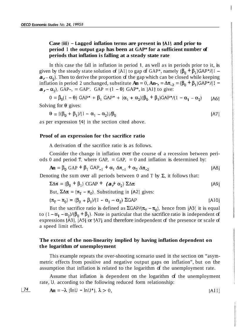
Case (iii) - Lagged inflation terms are present in lAll and prior to period 1 the output gap has been at GAP* for a sufficient number of periods that inflation is falling at a steady state rate

In this case the fall in inflation in period 1, as well as in periods prior to it, is given by the steady state solution of IAll to gap of GAP*, namely (Po + p,)GAP*/( I - a, - a>). Then to derive the proportion of the gap which can be closed while keeping inflation in period 2 unchanged, substitute An = 0, An-, = An-2 = (Po + P,)GAP*/( 1 - a, - a2), GAP-, = GAP‘. GAP = ( 1 - 0) GAP*, in lAl] to give:

Solving for 8 gives: o = p0(i - e) GAP* + pI GAP* + (a, + a,)(pO + ~ , ) G A P * / ( I - a, - a,)

8 = rcpo + PJU -a, -

1 ~ 6 1

IA71 as per expression 141 in the section cited above.

Proof of an expression for the sacrifice ratio

A derivation of the sacrifice ratio is as follows.

Consider the change in inflation over the course of a recession between peri-

lA8l

lA9 I But, CAn = (rr, - no). Substituting in IA2] gives:

“4101 But the sacrifice ratio is defined as CGAP/(TL,. - no), hence from IA3) it is equal

to ( 1 - a, - a,)/(Po + P I ) . Note in particular that the sacrifice ratio is independent of expressions IA3), \A51 or IA7) and therefore independent of the presence or scale of a speed limit effect.

ods 0 and period T. where GAP, = GAP, = 0 and inflation is determined by:

An = Po GAP + P I GAP-, + a, An-, + a2 AX-,

CAX = (Po + P I ) CGAP + (a, + a2) ZAZ

(? - no) = (Po + PI ) / ( I - a, - “2) CGAP

Denoting the sum over all periods between 0 and T by C, it follows that:

The extent of the non-linearity implied by having inflation dependent on the logarithm of unemployment

This example repeats the over-shooting scenario used in the section on “asymmetric effects from positive and negative output gaps on inflation”, but on the assumption that inflation is related to the logarithm of the unemployment rate.

Assume that inflation is dependent on the logarithm of the unemployment rate, U. according to the following reduced form relationship:

An = -1 (InU - ] n u * ) , h > 0, IAl1 I E


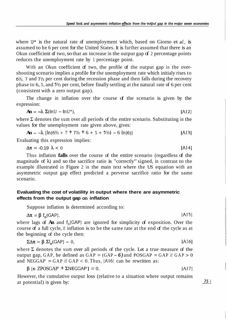
where U * is the natural rate of unemployment which, based on Giorno et al., is assumed to be 6 per cent for the United States. It is further assumed that there is an Okun coefficient of two, so that an increase in the output gap of 2 percentage points reduces the unemployment rate by 1 percentage point.

With an Okun coefficient of two, the profile of the output gap in the over- shooting scenario implies a profile for the unemployment rate which initialy rises to 6'/2, 7 and 7% per cent during the recession phase and then falls during the recovery phase to 6, 5, and 5% per cent, before finally settling at the natural rate of 6 per cent (consistent with a zero output gap).

The change in inflation over the course of the scenario is given by the expression:

An = -h C(1nU - InU*), IAl21 where C denotes the sum over all periods of the entire scenario. Substituting in the values for the unemployment rate given above, gives:

An = -h lln(6% + 7 + 7% + 6 + 5 + 5%) - 6 In(6)l 1 ~ 1 3 1 Evaluating this expression implies:

An = -0.19 h < 0 IA141 Thus inflation falls over the course of the entire scenario (regardless of the

magnitude of A) and so the sacrifice ratio is "correctly" signed, in contrast to the example illustrated in Figure 2 in the main text where the US equation with an asymmetric output gap effect predicted a perverse sacrifice ratio for the same scenario.

Evaluating the cost of volatility in output where there are asymmetric effects from the output gap on inflation

Suppose inflation is determined according to:

An = p f,(GAP), IAl51 where lags of An and f,(GAP) are ignored for simplicity of exposition. Over the course of a full cycle, if inflation is to be the same rate at the end of the cycle as at the beginning of the cycle then:

CAE = p Zf,(GAP) = 0, IA161 where C denotes the sum over all periods of the cycle. Let a true measure of the output gap, GAP, be defined as GAP = (GAP - 6 ) and POSGAP = GAP if G A P > 0 and NEGGAP' = G A P if G A P < 0. Thus, IA16] can be rewritten as:

"A.171 However, the cumulative output loss (relative to a situation where output remains at potential) is given by:

p In ZPOSGAP' + ZNEGGAP'] = 0.


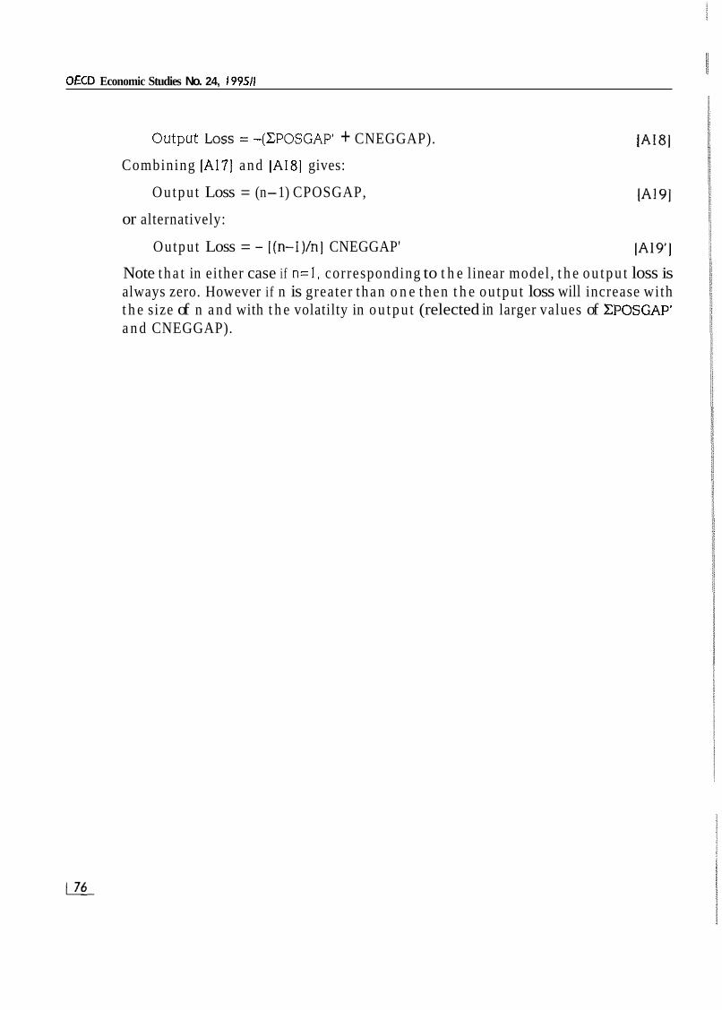
Output Loss = -(CPOSGAP + CNEGGAP). [A181 Combining [A171 and [A181 gives:

Ou tpu t Loss = (n-1) CPOSGAP,

or alternatively:

Output Loss = - l(n-l)/n] CNEGGAP' IA19'I

Note t h a t in either case if n = l , corresponding to t h e linear model , t h e o u t p u t loss is always zero. However if n is greater than o n e then t h e ou tpu t loss will increase with t h e size of n a n d with t h e volatilty in o u t p u t (relected in larger values of ZPOSGAP' a n d CNEGGAP).

Annex 2

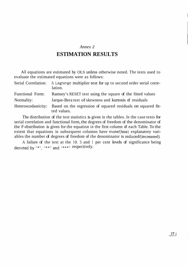
ESTIMATION RESULTS

All equations are estimated by OLS unless otherwise noted. The tests used to evaluate the estimated equations were as follows: Serial Correlation: A Lagrange multiplier test for up to second order serial corre-

lation. Functional Form: Ramsey’s RESET test using the square of the fitted values Normality: Jarque-Bera test of skewness and kurtosis of residuals Heteroscedasticity: Based on the regression of squared residuals on squared fit-

ted values. The distribution of the test statistics is given in the tables. In the case tests for

serial correlation and functional form, the degrees of freedom of the denominator of the F-distribution is given for the equation in the first column of each Table. To the extent that equations in subsequent columns have more/(less) explanatory variables the number of degrees of freedom of the denominator is reduced!(increased).

A failure of the test at the 10. 5 and 1 per cent levels of significance being denoted by “*’,, ,,**’, and ‘,**I” respectively.


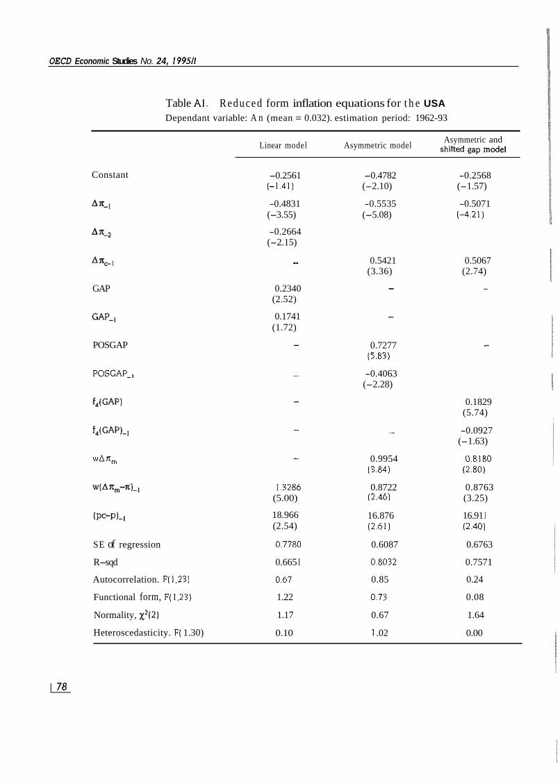
Table Al . Reduced form inflation equations for t h e USA Dependant variable: A n (mean = 0.032). estimation period: 1962-93

Constant

GAP

POSGAP

POSGAP-,

wAn,

Asymmetric and Linear model Asymmetric model gap model

-0.2561 -0.4782 -0.2568 (-1.41) (-2.10) (-1.57)

(-3.55) (-5.08) (4 .21) -0.4831 -0.5535 -0.5071

-0.2664 (-2.15)

- 0.5421 0.5067 (3.36) (2.74)

0.2340 (2.52)

0.1741 (1.72)

0.7277 (5.83)

- -0.4063 (-2.28)

0.1829 (5.74)

(-1.63) - -0.0927

0.9954 0.8180 (3.84) (2.80)

I .3286 0.8722 0.8763 (5.00) 12.46) (3.25)

18.966 (2.54)

16.876 16.91 I (2.61) (2.40)

SE of regression 0.7780 0.6087 0.6763

R-sqd 0.665 I 0.8032 0.7571

Autocorrelation. F(1.23) 0.67 0.85 0.24

Functional form, F( I .23) 1.22 0.73 0.08

Normality, x2(2) 1.17 0.67 1.64

Heteroscedasticity. F( 1.30) 0.10 I .02 0.00


Table A2. Reduced form inflation equations for japan Dependant variable: A n (mean = -0.181). estimation period: 1966-93

Asymmetric and shifted gap model Linear model Asymmetric model

Constant

A X ,

GAP

POSGAP

f,(GAPl

Ana-1

''=SO

SE of regression

R-Sqd

Autocorrelation. F( I .22)

Functional form, F( I .22)

Normality. x2(2)

Heteroscedasticity. F( I .26)

-0.3458 (-1.04)

-0.8396 (-2.82)

0.4548 (2.61)

-

-

0.6700 (2.49)

0.0534 (7.93)

1.7477

0.7859

0.39

0.64

1.37

0.00

-0.9094 (-2.34)

-0.8541 (-2.98)

-

0.7427 (3.00)

-

0.6881 (2.65)

0.0549 (8.52)

1.6857

0.8009

0.54

0.72

0.33

0.17

-0.3537 (-I. 13)

-0.8420 (-3.03)

-

-

0.2333 (3.32)

0.6746 (2.68)

0.0542 (8.66)

I .6362

0.8 I24

0.35

0.58

0.40

0.09


Table A3. Reduced form inflation equations for Western Germany Dependant variable: An (mean = -0.0331, estimation period: 1963-93

Constant

GAP

POSGAP

NECGAP

D70


-0.3679 4 .5157 4.3192 (-2.50) (-1.97) (-2.20)

4.2858 -0.2724 -0.2203 (-3.66) 1-2.52) (-2.53)

-0.3921 4 .3880 4 .3836 (-3.66) (-4.17) ( 4 . 4 5 )

0.2248 - (2.41)

0.1211 (1.02)

0.3687 (2.40)

0. 1805 (1.11)

- 0.2031 (3.75)

0.1967 0.2634 (1.47) (2.21)

0.2696 (2.33)

6.6794 6.7 184 6.76 I4 (8.34) (8.26) (8.60)

SE of regression 0.7752 0.7851 0.7638

R-sqd 0.8412 0.8371 0.8388

Autocorrelation. F( 1.24) 2.53 4.02' 2.00

Functional form. F( 1,24) 0.06 0.88 0.19

Normality, x2(2) 0.91 3.14 I .72

Heteroscedasticity. F( 1.29) 0.42 0.51 0.21


Table A4. Reduced form inflation equations for France Dependant variable: An (mean = -0.062). estimation period: 1965-93


Constant

GAP

GAP-,

POSGAP

POSGAP-I

NEGGAP-I

f,(GAP)

f,lGAPl-,

wAnm

(nC-n)-,

D6869

SE of regression

R-sqd

Autocorrelation. F( 1.22)

Functional form, F( 1.22)

Normality, x2(2)

Heteroscedasticity F( 1.27)

-0.2391 (-1.24)

0.1584 (0.96)

0.4443 (2.61)

-

-

-

-

-

0.1045 (2.88)

0.7239 (3.30)

2.3717 (3.26)

0.9490

0.6421

I .29

0.98

0.97

1.57

4.3744 (-1.11)

-

-

0.3247 (1.16)

0.3727 (1.34)

-0.4699 (1.52)

-

-

0.1047 (2.92)

0.7449 (3.35)

2.4034 (3.24)

0.9606

0.6496

1.29

1.77

0.78

I .40

-0.1822 (-0.97)

-

-

-

-

-

0.1399 (1.21)

0.2733 (2.35)

0.1026 (2.86)

0.7522 (3.45)

2.2973 (3.19)

0.9473

0.6437

1.25

0.37

0.98

0.93


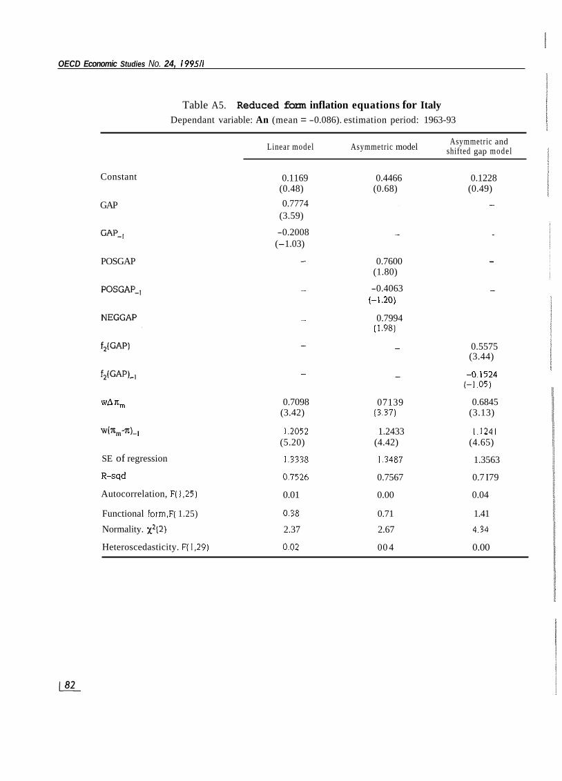
Table A5. Reduced form inflation equations for Italy Dependant variable: An (mean = -0.086). estimation period: 1963-93

~


Constant

GAP

GAP-,

POSGAP

wA nm

wm,-z)_,

SE of regression

Rsqd

Autocorrelation, F( 1,251

0.1169 0.4466 0.1228 (0.48) (0.68) (0.49) 0.7774 -

(3.59)

-0.2008 - - (-1.03)

-

0.7600 (1.80)

- -0.4063 - (-I .20)

( I .98) - 0.7994

- 0.5575 - (3.44)

(-1.05) - -0.1524 -

0.7098 07139 0.6845 (3.42) (3.37) (3.13)

1.2052 1.2433 1.1241

1.3338 1.3487 1.3563

0.7526 0.7567 0.7 I79

0.01 0.00 0.04

(5.20) (4.42) (4.65)

Functional form.F( 1.25) 0.38 0.71 1.41

Normality. ~ ~ ( 2 ) 2.37 2.67 4.34

Heteroscedasticity. F( I .29) 0.02 0 0 4 0.00


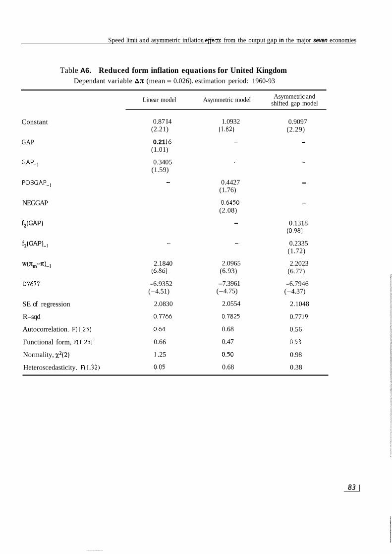
Table A6. Reduced form inflation equations for United Kingdom Dependant variable An (mean = 0.026). estimation period: 1960-93


Constant

GAP

GAP-,

POSGAP-,

NEGGAP

f2(GAP)

f,(GAP)L

w ( ~ m - ~ ) - ]

D7677

SE of regression

R-sqd

Autocorrelation. F( I .25)

Functional form, F(1.25)

Normality, x2(2)

Heteroscedasticity. F( I ,32)

0.87 I4 (2.21)

0.21 16 (1.01)

0.3405 (1.59)

-

-

-

-

2.1840 (6.86)

-6.9352 (-4.51)

2.0830

0.7766

0.64

0.66

I .25

0.05

1.0932 ( I .82)

-

-

0.4427 (1.76)

0.6450 (2.08)

-

-

2.0965 (6.93)

-7.3961 (-4.75)

2.0554

0.7825

0.68

0.47

0.50

0.68

0.9097 (2.29)

-

-

-

-

0.1318 (0.98)

0.2335 (1.72)

2.2023 (6.77)

-6.7946 (-4.37)

2.1048

0.77 I9

0.56

0.53

0.98

0.38

OECD Economic Studies No. 24, I995I1

Table A7. Reduced form inflation equations for Canada Dependant variable: Ax (mean = 0.015). estimation period: 1962-93

Constant

GAP

POSGAP

m-m-,

AIB

SE of regression

Asymmetric and shifted aaD model Linear model Asymmetric model

1.0887 (3.52)

0.4123 (3.64)

-

0.3386 1.1731 (1.13) (4.101

0.9588 (4.85)

1.8420 2.0749 (5.02) 16.31)

1.8525 2.4000 (4.36) (5.93)

0.25 12 (4.56)

2.0306 (6.02)

2.2469 (5.53)

0.6496 0.5376 0.5980 (3.801 (3.71 1 (3.95)

-4.4692 -4.6872 -4.431 I (-4.32) (-5.08) (-4.74)

I .409 1 1.2550 1.2903

R-sqd 0.7 I90 0.7771 0.7644

Autocorrelation. F( 1.25) 2.22 0.00 0.90

Functional form, F( I .25) 0.33 0.56 0.43

Normality. ~ ~ ( 2 ) 0.69 0.40 1.95

Heteroscedasticity. F( 1,30) 0.16 0.66 0.16


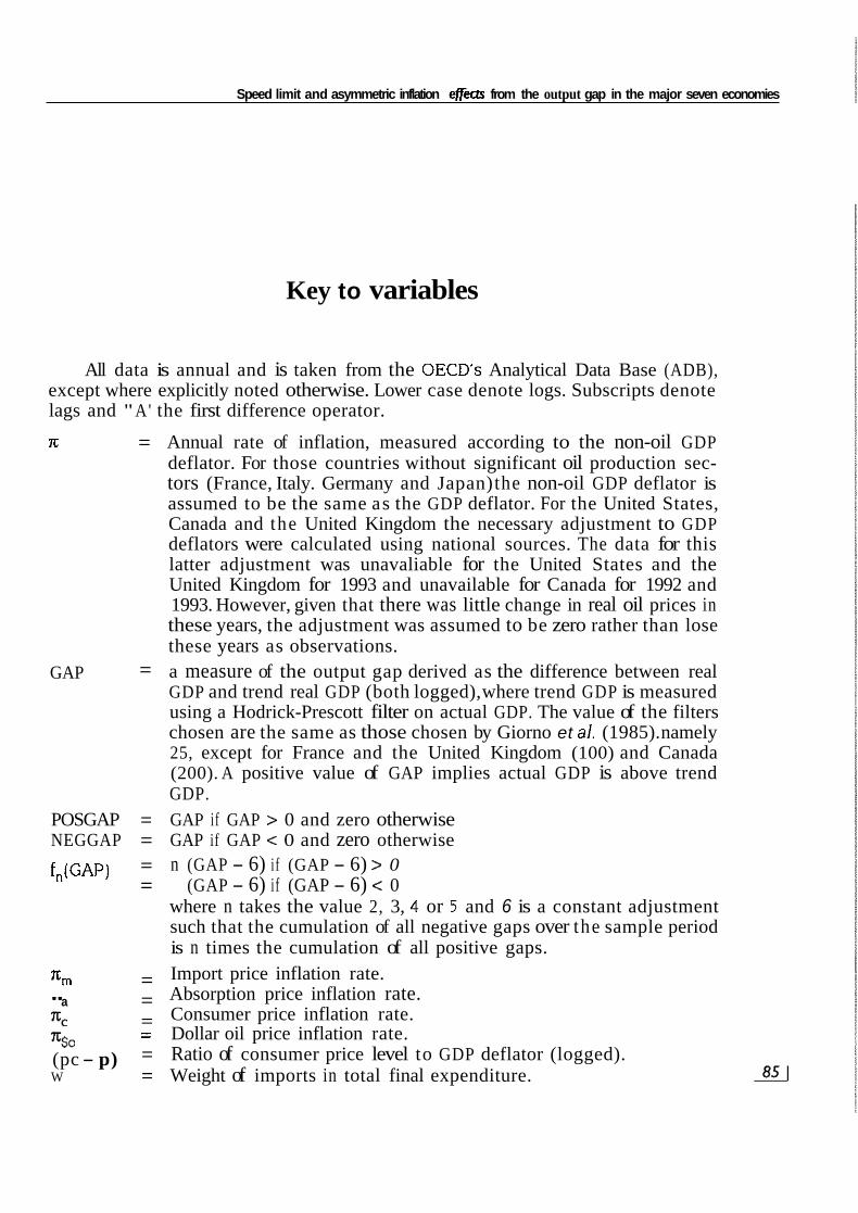
Key to variables

All data is annual and is taken from the OECD's Analytical Data Base (ADB), except where explicitly noted otherwise. Lower case denote logs. Subscripts denote lags and "A' the first difference operator.

7.c = Annual rate of inflation, measured according to the non-oil GDP deflator. For those countries without significant oil production sectors (France, Italy. Germany and Japan) the non-oil GDP deflator is assumed to be the same as the GDP deflator. For the United States, Canada and the United Kingdom the necessary adjustment to GDP deflators were calculated using national sources. The data for this latter adjustment was unavaliable for the United States and the United Kingdom for 1993 and unavailable for Canada for 1992 and 1993. However, given that there was little change in real oil prices in these years, the adjustment was assumed to be zero rather than lose these years as observations. a measure of the output gap derived as the difference between real GDP and trend real GDP (both logged), where trend GDP is measured using a Hodrick-Prescott filter on actual GDP. The value of the filters chosen are the same as those chosen by Giorno et al. (1985). namely 25, except for France and the United Kingdom (100) and Canada (200). A positive value of GAP implies actual GDP is above trend GDP.

GAP =

POSGAP = GAP if GAP > 0 and zero otherwise NEGGAP = GAP if GAP < 0 and zero otherwise f,(GAP) = n (GAP - 6) if (GAP - 6) > 0

= (GAP - 6) if (GAP - 6) < 0 where n takes the value 2, 3, 4 or 5 and 6 is a constant adjustment such that the cumulation of all negative gaps over the sample period is n times the cumulation of all positive gaps.

"m = Import price inflation rate. "a = Absorption price inflation rate. % = Consumer price inflation rate.

= Dollar oil price inflation rate. 7% (pc - p) = Ratio of consumer price level to GDP deflator (logged). W = Weight of imports in total final expenditure.

OECD Economic Swdies No. 24, 199511

DWxx

A1 B = Dummy for operation of Anti-Inflation Board [Canada).

= Dummy variable taking the value unity in years 19yy and 19xx and zero elsewhere.

B,

BIBLIOGRAPHY

LL and MANKIW (I 994), “Asymmetric Price Adjustment an’ Economic Journal, I04 (March), 247-26 I.

Economic Fluctuations”,

BARRELL R. ( I 990). “Has the EMS Changed Wage and Price Behaviour in Europe ?”, National Institute Economic Review, November.

CHADA, B., P. MASSON and G. MEREDITH (I 992), “Models of inflation and the costs of Disinflation”, IMF StafPapers, Vol. 39, No. 2.

COLETTI, D., B. HUNT, D. ROSE and R. TETLOW (1994), “Some Dynamic Properties of QPM”, Bank of Canada, mimeo.

DE LONG, J.B. and L.H. SUMMERS (1988), “How does Macroeconomic Policy Effect Out- put”, Brookings Papen on Economic Activity, 2, pp. 433-494.

ELMESKOV, J. (1993), “High and Persistent Unemployment: Assessment of the Problem and i t s Causes”, OECD Economics Department Working Paper, No. 132, Paris.

GIORNO, C., P. RICHARDSON, D. ROSNEARE, P. VAN DEN NOORD (1995), “Estimat- ing Potential Output, Output Gaps and Structural Budget Balances”, OECD Economics Department Working Papers, No. 152, Paris.

LAXTON, D., D. ROSE, and R. TETLOW (19930), “Problems in Identifying Non-Linear Phillips Curves: Some Further Consequences of Mismeasuring Potential Output”, Bank of Canada, Working Paper 93-6.

LAXTON, D., D. ROSE, and R. TETLOW (1993b). “Is the Canadian Phillips Curve Non- Linear?”, Bank of Canada, Working Paper 93-7.

LAXTON, D., G. MEREDITH and D. ROSE, (I 994). “Asymmetric Effects of Economic Activity on Inflation: Evidence and Policy Implications”, IMF Working Paper.

OECD (I 99 I), OECD Economic Outlook, No. 50, Paris, December.

OECD (1994a), “The OECD Jobs Study, Part I, Labour Markets and Underlying Forces of

OECD (1994), OECD Economic Outlook, No. 56, Paris, December.

TORRES, R. and J.P. MARTIN (I 990). “Measuring Potential Output in the Seven Major OECD Countries”, OECD Economic Studies, No. 14, Paris.

TURNER, D, K.F. WALLIS and J.D. WHITLEY, “Using Macroeconometric Models to evaluate Policy Proposals”, in “Policymaking with Macroeconomic Models”, ed. A. Britton,

Change”, Paris.

Cower. 871

speed limit and asymmetric inflation effects … · oecd economic studies no. 24, i995/1 speed...

Documents