1

ABSTRACT

The total transition rate summed over all decay channels can be measured

either through frequency-resolved studies of the level width, or through

time-resolved studies of the level lifetime. In order to determine the natural

line width in a field-free spectroscopic measurement, either the lifetime must

be very short, or the Doppler, pressure, and instrumental broadenings must

be made very small. Line widths have been determined using Fabry-Perot

spectrometry at very low temperatures and pressures, and in beam-foil

studies of radioactive transitions in which the lower level decays very

rapidly via auto-ionisation. The line-width can also be determined through

the use of the phase shift method. Here modulated excitation is applied to

the source, thus producing similarly modulated emitted radiation, and the

width can be specified from the phase shift between the two signals. Other

methods involve resonance fluorescence techniques, where sub-Doppler

widths are obtained because the width of the exciting radiation selects a

subset of particle motions within the sample. Resonance fluorescence

techniques that can be used to determine level widths include zero-field level

crossing (the Hanle effect), high-field level crossing, and double optical

resonance methods, but the Hanle effect is the most common.

2

INTRODUCTION

TIME-RESOLVED DECAY MEASUREMENTS

The most direct method for the experimental determination of level lifetimes

is through the time-resolved measurement of free decay of the fluorescence

radiation following a cut-off of the source of excitation. An important factor

limiting the accuracy is the repopulation of the level of interest by cascade

transitions from higher-lying levels. For this reason, decay curve

measurements fall into two classes: those that involve selective excitation of

the level of interest, thus eliminating cascading altogether; and those that use

correlations between cascades connected decays to account for the effects of

cascades.

SELECTIVE EXCITATION

Lifetime measurements accurate to within a few parts in 103 have been

obtained through selective excitation produced when appropriately tuned

laser light is incident on a gas cell or a thermal beam, or on a fast ion beam.

With a gas cell or thermal beam, the timing is obtained by a pulsed laser and

delayed coincidence detection. With a fast ion beam, time-of-flight methods

are used. In either case, after removal of the background, the decay curve of

intensity vs. time is a single exponential, and the lifetime is obtained from its

semi logarithmic slope. Laser-excited time-of-flight studies were first

3

carried out by observing the optical decay of the ion in light following

excitation using a laser beam, which crossed the ion beam. In these studies,

the laser light was tuned to the frequency of the desired absorption transition

either through the use of a tunable dye laser, or by varying the angle of

intersection to exploit the Doppler effect. Recent measurements have

utilised diode laser excitation in this geometry.

A number of adaptations of this technique have been developed in which the

laser and ion beams are made to be collinear, and are switched into and out

of resonance within a segment of the beam by use of the Doppler effect.

The collinear geometry can provide a longer excitation region and less

scattering of laser light into the detector than occurs in the crossed beam

geometry. In one adaptation, excitation occurs within an electrostatic

velocity switch, and the time resolution is obtained by physically moving the

velocity switch. In another adaptation the ion beam is accelerated with a

spatially varying voltage ramp. The resonance region is moved relative to a

fixed detector by time-sweeping either the laser tuning or the ramp voltage.

While these selective excitation methods totally eliminate the effects of

cascade repopulation, they are generally limited to levels in neutral and

singly ionised atoms that can be accessed from the ground state by strongly

absorptive E1 transitions, and the selectivity itself is a limitation. Many very

4

precise measurements have been made by these techniques, but they have

primarily involved ¨Q = 0 resonance transitions in neutral alkali atoms and

singly ionised alkali-like ions.

NONSELECTIVE EXCITATION

Much more general access can be obtained by non-selective excitation

methods, such as pulsed electron beam bombardment of a gas cell or gas jet,

or in-fight excitation of a fast ion beam by a thin foil. Pulsed electron beam

excitation can be achieved either through use of a suppressor grid, or by

repetitive high frequency deflection of the beam across a slit so as to chop

the beam. Particularly in the case of weak lines, the high frequency

deflection technique offers the advantages of high current and sharp cut-off

times. The high currents yield high light levels, so that high-resolution

spectroscopic methods can be used to eliminate the effects of line blending.

Pulsed electron excitation methods are well suited to measurements in

neutral and near neutral ions (although for very long lifetimes in ionised

species, the decay curves can be distorted if particles escape from the

viewing volume through the Coulomb explosion effect).

However, for highly ionised atoms, the only generally applicable method is

thin foil excitation of a fast ion beam. Nonselective excitation techniques

can also be applied to measurements such as the phase shift method and the

5

Hanle effect, in which case cascade repopulation also can become a serious

problem. However, most of the attempts to eliminate or account for cascade

effects have occurred in decay curve studies.

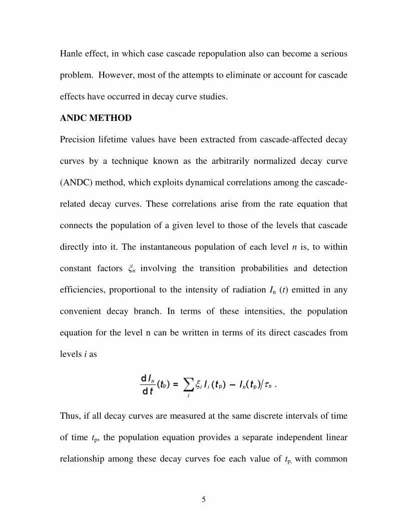
ANDC METHOD

Precision lifetime values have been extracted from cascade-affected decay

curves by a technique known as the arbitrarily normalized decay curve

(ANDC) method, which exploits dynamical correlations among the cascade-

related decay curves. These correlations arise from the rate equation that

connects the population of a given level to those of the levels that cascade

directly into it. The instantaneous population of each level n is, to within

constant factors �n involving the transition probabilities and detection

efficiencies, proportional to the intensity of radiation In (t) emitted in any

convenient decay branch. In terms of these intensities, the population

equation for the level n can be written in terms of its direct cascades from

levels i as

Thus, if all decay curves are measured at the same discrete intervals of time

of time tp, the population equation provides a separate independent linear

relationship among these decay curves foe each value of tp, with common

6

constant coefficients given by the lifetime 2n and the normalization

parameters �i. Although the sum over cascades is formally unbounded, the

dominant effects of cascading from highly excited states are often accounted

for by indirect cascading through the lower states, in which case the sum can

be truncated after only a few terms. ANDC analysis consists of using this

equation to relate the measured Ik(tp) (using numerical differentiation or

integration) to determine 2k and the �i through a linear regression. If all

significant direct cascades have been included, the goodness-of-fit will be

uniform for all time sub-regions, indicating reliability. If important cascades

have been omitted or blends are present, the fit will vary over time sub

regions, indicating a failure of the analysis. Very rugged algorithms have

been developed that permit accurate lifetimes to be extracted even in cases

where statistical fluctuations are substantial, and studies of the propagation

and correlation of errors have been made. Clearly the ANDC method is most

easily applied to systems for which repopulation effects are dominated by a

small number of cascade channels.

There are three rather different ways of measuring lifetimes of excited states:

delay time, beam foil spectroscopy, and Hanle effect. None of these

methods is universally applicable. Some work only for states that can be

7

excited directly from the ground state, others are no good if the lifetime is

too short (strong line) or the intensity too low (weak line) for accurate

measurement. Amongst them, however, they cover a very wide range of

transitions, both atomic and molecular, and they have in common the one

immensely important advantage that there is no need to know the population

of the initial level. It must be remembered that a lifetime does not yield

directly an oscillator strength, unless there is only one allowed transition

from the excited state. However, if relative values of A2j can be obtained

from emission, they can be put on an absolute scale by a measurement of 2.

(where A2j is the Einstein coefficient for spontaneous emission and 2 is the

time constant).

In the description of the delay methods that follows (and also in that of the

Hanle effect) reference is made to excitation by resonance radiation. It is

now becoming possible to use tuneable dye laser as an exciting source. Its

high intensity makes it ideal for selective population of excited levels, and

its short pulse duration allows good time resolution. New ways of

exploiting these advantages are constantly being devised at the present time.

8

1. DELAY METHODS

The delayed coincidence method is shown schematically below (Figure 1).

The gas is excited by a pulsed electron beam (or occasionally by a pulse of

resonance radiation), which also triggers off the time-to-pulse-height

converter. The stop signal for this is provided by the emitted radiation, via a

monochromator and photo-multiplier, so that the pulse height is proportional

to the time between the excitation and decay of the relevant excited level.

Building up statistics for dN/dt as a function of t should result in an

exponential of time constant 2.

Figure 1. Schematic arrangement for measurement of lifetimes by

delayed coincidence

9

A variant of this is to use a coincidence counter in place of the time-to-

pulse-height converter and to record coincidences between the exciting

electron pulse and the emitted radiation as a function of a variable delay time

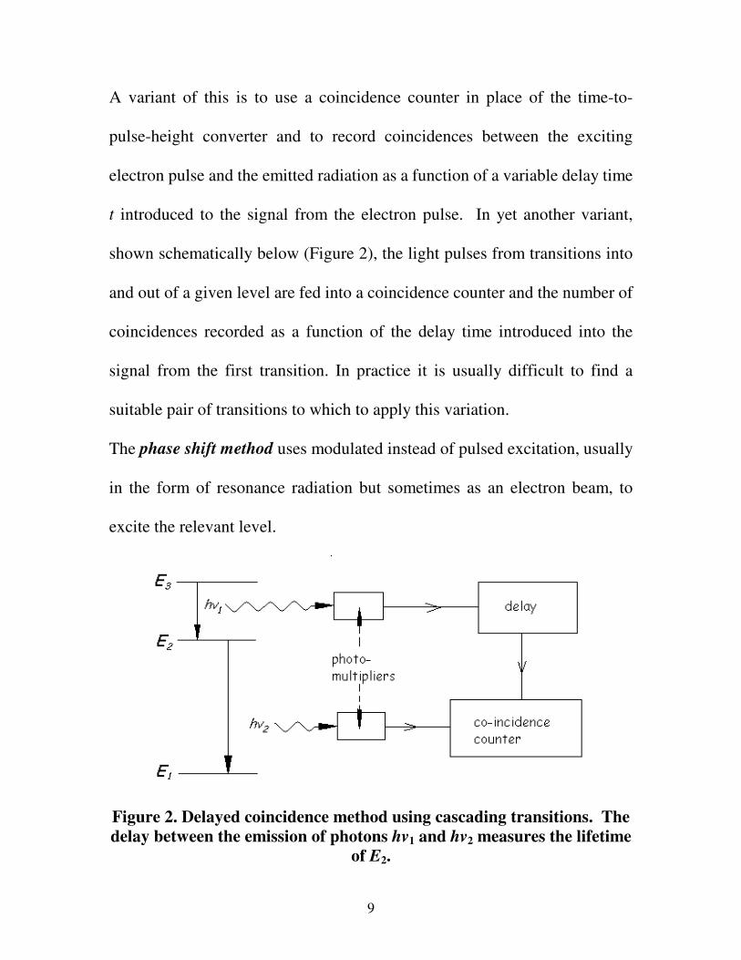
t introduced to the signal from the electron pulse. In yet another variant,

shown schematically below (Figure 2), the light pulses from transitions into

and out of a given level are fed into a coincidence counter and the number of

coincidences recorded as a function of the delay time introduced into the

signal from the first transition. In practice it is usually difficult to find a

suitable pair of transitions to which to apply this variation.

The phase shift method uses modulated instead of pulsed excitation, usually

in the form of resonance radiation but sometimes as an electron beam, to

excite the relevant level.

Figure 2. Delayed coincidence method using cascading transitions. The

delay between the emission of photons hv1 and hv2 measures the lifetime

of E2.

10

The emitted radiation is then also modulated, but with a phase shift θ

relative to the exciting radiation which depends on the lifetime of the excited

state according to tanθ = 2πvm2, where vm is the modulating frequency. The

figure below (Figure 3) shows the method schematically. The modulation

may be done with a Kerr cell or with a standing ultrasonic wave. The

accuracy can be improved by modulating the voltage on the photo-multiplier

cathode so that θ is measured at the beat frequency of a few kilocycles rather

than at the modulation frequency, which has to be in the megacycle range.

The delay methods can be used for lifetimes from a few microseconds to a

few nanoseconds. Apart from difficulties associated with scattered light and

insufficient resolution (they are usually used with broad band-pass

monochromators or filters to obtain enough intensity in the fluorescent

light), they have two principal potential sources of error. The first is

cascading: unless the relevant level is excited by resonance radiation or by a

tuned dye laser, a number of higher levels may be excited at the same time

and subsequently decay to the level under investigation. The latter is

therefore re-populated from above, so that its apparent lifetime is prolonged.

In principle, even with electron excitation it should be possible to excite only

the required level, but in practice the cross-section near the threshold energy

is so small that considerably higher electron energies have to be used. The

11

second principal difficulty affects all levels emitting to the ground or a

metastable state and is usually known as imprisonment of radiation.

Figure 3. Schematic arrangement for measurement of lifetime by phase

shift.

If the gas is not optically thin, a number of photons will be absorbed and re-

emitted one or more times before they eventually get out, and the effect is,

again, to prolong the apparent lifetime of the excited state. Measuring

apparent lifetime as a function of pressure can check for the effect. A

further source of error that may affect the longer-lived states is collisional

depopulation; this of course shortens the apparent lifetime. Both these last

12

troubles may be avoided by going to sufficiently low pressures (atomic

beams have been used for this reason), but one may then run into difficulties

with the low light intensities. The accuracy claimed for lifetime

measurements is usually around 10%, is often better, but may in fact be

considerably worse if systematic errors have not been eliminated.

2. BEAM FOIL METHOD

A beam of ions of various degrees of ionisation emerges from the thin foil in

different states of excitation. The excited states decay as the beam travels

downstream from the foil, and the rate of decrease of intensity of any

particular line as a function of distance from the foil gives directly the

lifetime of the relevant excited state.

Historically, this method is the successor to the experiments of Wien in

1920s with canal rays, in which the lifetime was measured from the decay of

emitted radiation as the excited ions in a discharge tube travelled beyond the

cathode. In practice, in the beam foil method, the spectrometer is kept fixed,

and the intensity of the required lines is measured while the foil is moved

upstream. It is necessary to monitor the constancy of the beam while this is

going on, either by measuring the total charge collected at its end or by using

a second photo-multiplier.

13

Figure 4. Reason for Doppler broadening in beam foil spectroscopy.

The excited ions have a velocity component in the R-direction of νν sin θθ

away from the spectrometer, giving a red-shift. For the B-direction

there is an equal blue shift.

The principal difficulties of the method are cascading from higher excited

states, low light intensity, and large Doppler broadening. The reason for this

last is illustrated above (Figure 4). The velocity of the beam is of order

5x108 cm sec

-1, and because of the finite acceptance angle of the

spectrometer the direction of observation is not strictly perpendicular to the

beam direction. For light travelling along ray B the ions have a component

of velocity along B of v sin θ, resulting in a blue shift, whereas for ray R the

velocity is v sinθ away from the spectrometer, giving a red shift. Since all

rays in the cone RB contribute to the image, the result is a broadened line.

14

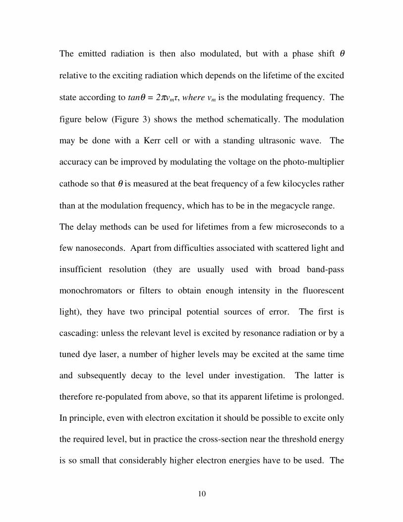
The low intensity makes a wide aperture essential, and the Doppler

broadening may be as high as

On the other hand, the density in the beam is so low that there are no

difficulties with imprisonment of radiation or collisional depopulation.

More importantly, this is the only method other than that of emission line

intensity, which can be applied to ionic spectra. It is best suited for lifetimes

of about 10-8

sec, during which time the ions travel a few cm. With shorter

lifetimes the decay is too fast to measure accurately, bearing in mind that it

is usually necessary to accept light from an appreciable length of beam ∆l to

obtain sufficient intensity, so that the space resolution is rather poor. If the

lifetime is very long, so few ions decay in the path ∆l that inadequate

intensity again becomes a problem.

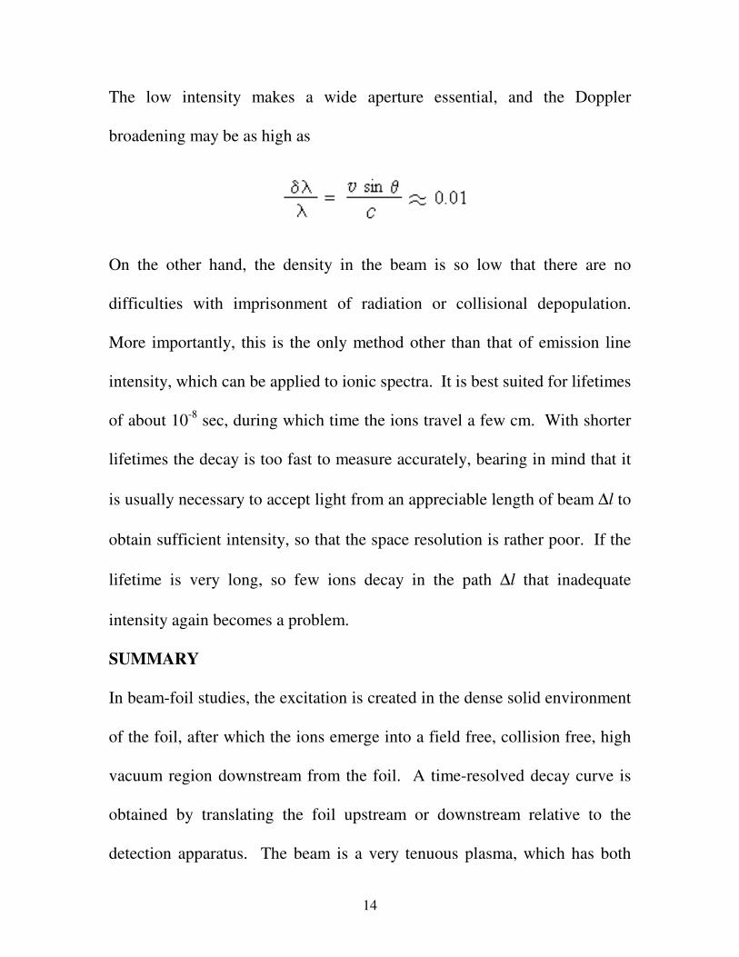
SUMMARY

In beam-foil studies, the excitation is created in the dense solid environment

of the foil, after which the ions emerge into a field free, collision free, high

vacuum region downstream from the foil. A time-resolved decay curve is

obtained by translating the foil upstream or downstream relative to the

detection apparatus. The beam is a very tenuous plasma, which has both

15

advantages and disadvantages. The low density avoids the effects of

collisional de-excitation and radiation trapping, but also produces relatively

low light levels. This requires fast optical systems with a corresponding

reduction in wavelength dispersion, and care must be taken to avoid

blending of these Doppler broadened lines. Methods have been developed

by which grating monochromators can be refocused to a moving light

source, thus utilizing the angular dependence of the Doppler effect to narrow

and enhance the lines.

3. HANLE EFFECT

This technique again is a resurrection from the 1920s, when the effect,

investigated by Hanle, was known as magnetic depolarisation of resonance

radiation. It is now also known as zero-field level crossing, being a special

case of the level-crossing experiments for the measurement of hyperfine

structure. For a very brief qualitative description of the effect it is simplest

to use a semi-classical model, but when there is hyperfine structure or close

fine structure in the excited level a proper quantum-mechanical treatment is

required. A typical experimental layout is shown below (Figure 5). Light

from the source of resonance radiation travelling in the y-direction is plane-

polarized in the x-direction before entering the resonance vessel where it is

absorbed and re-emitted. The emitted radiation has the same polarization as

16

the exciting radiation, and a photo-multiplier on the x-axis therefore records

no signal. If now a magnetic field is applied to the resonance vessel in the z-

direction, the resonance radiation is partly de-polarized, and a signal is

registered, rising at strong field to half the intensity in the absence of the

polariser.

Figure 5. Schematic arrangement for Hanle effect. The photomultiplier

in the x-direction registers a signal where field B is applied in the z-

direction.

This is because the direction of oscillation of the electrons, originally

parallel to the x-axis, now precesses about the z-axis. If the precession is

sufficiently rapid, half the oscillations may be considered as in the y-

direction, thus radiating in the x-direction. The lifetime enters into the story

17

because if the precession is not very fast some of the atoms will have

decayed before the precessional cycle is completed, so that the intensity

component in the y-direction is less than the original x-component.

Figure 6. Classical interpretation of Hanle effect. (a) represents small

damping (ωωB>1/ττ) and (b) represents large damping �&Ba��ττ). The

length of each spoke in these figures is proportional to the intensity of

the radiation at the corresponding direction of polarization.

The signal thus depends on the relative magnitudes of the precessional and

decay times, as shown schematically above (Figure 6): (a) represents the

situation when the precessional frequency ωB is large compared to the

damping constant γ = 1/τ and (b) shows them comparable. Simply by

treating the system as an oscillator precessing with angular frequency ωB and

decaying amplitude exp (- ½ γ / t) it can be shown that the signal is given by

18

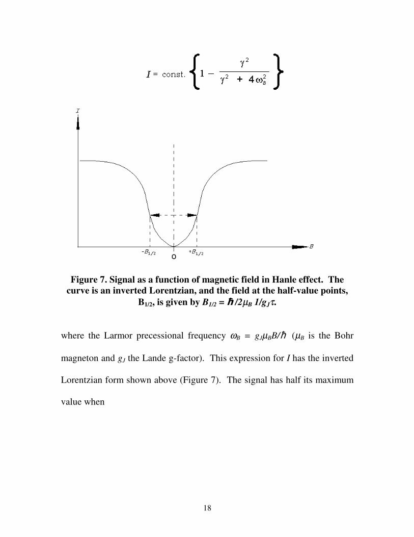
Figure 7. Signal as a function of magnetic field in Hanle effect. The

curve is an inverted Lorentzian, and the field at the half-value points,

B1/2, is given by B1/2 = Y /2µµB 1/gJττ.

where the Larmor precessional frequency ωB = gJµBB/Y (µB is the Bohr

magneton and gJ the Lande g-factor). This expression for I has the inverted

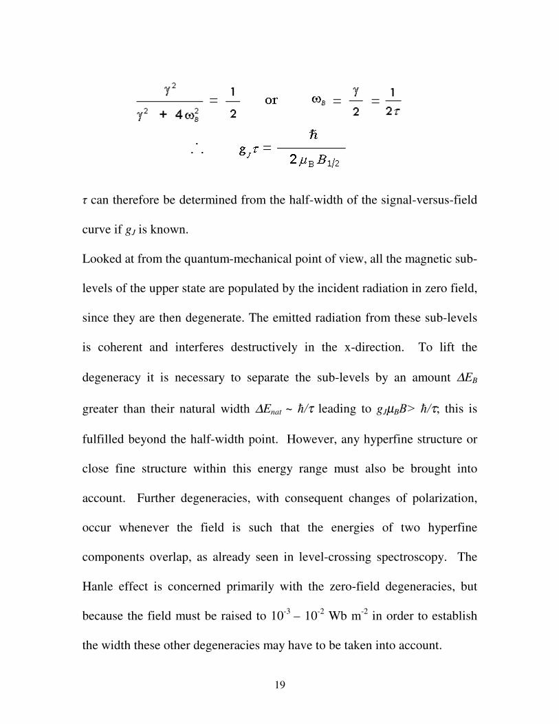
Lorentzian form shown above (Figure 7). The signal has half its maximum

value when

19

2 can therefore be determined from the half-width of the signal-versus-field

curve if gJ is known.

Looked at from the quantum-mechanical point of view, all the magnetic sub-

levels of the upper state are populated by the incident radiation in zero field,

since they are then degenerate. The emitted radiation from these sub-levels

is coherent and interferes destructively in the x-direction. To lift the

degeneracy it is necessary to separate the sub-levels by an amount ∆EB

greater than their natural width ∆Enat ~ ��τ leading to gJµB%!���τ; this is

fulfilled beyond the half-width point. However, any hyperfine structure or

close fine structure within this energy range must also be brought into

account. Further degeneracies, with consequent changes of polarization,

occur whenever the field is such that the energies of two hyperfine

components overlap, as already seen in level-crossing spectroscopy. The

Hanle effect is concerned primarily with the zero-field degeneracies, but

because the field must be raised to 10-3

– 10-2

Wb m-2

in order to establish

the width these other degeneracies may have to be taken into account.

20

In contrast to the other lifetime techniques, this one has no cascading

problems. The ‘line width’ is determined entirely by the lifetime, with no

Doppler or power broadening. Apart from limitations on the possible

transitions to which the method can be applied, the main difficulties are

associated with self-absorption in the original resonance source and

coherence narrowing of the ‘line’, resulting from coherent trapping of the

radiation.

SUMMARY

In its most commonly used form, the Hanle effect makes use of polarized

resonance radiation to excite atoms in the presence of a known variable

magnetic field. The magnetic substates of the sample are anisotropically

excited, and the subsequent radiation possesses a preferred angular

distribution. By applying the magnetic field in a direction perpendicular to

the anisotropy, the angular distribution is made to precess, producing

oscillations in the radiation observed at a fixed angle. At infinite

precessional frequency the intensity would be proportional to the

instantaneous average angular intensity, by at finite precessional frequency it

depends upon the decay that has occurred during each quarter rotation.

Measured as a function of magnetic field, the emitted intensity has a

21

Lorentzian shape centered about zero field with a width that depends on the

lifetime and g-factor of the level.

22

REFERENCES

1. Thorne A. P. (1974) Experimental determination of transition

probabilities, Spectrophysics, Chapman and Hall & Science Paperbacks,

London, 332.

2. Curtis L. J. Lifetimes: In Part B, 17, Precision Oscillator Strength and

Lifetime Measurements, 262,

http://www.physics.utoledo.edu/~ljc/drake17.pdf, Department of Physics

and Astronomy, University of Toledo, Toledo, Ohio 43606.

23

BIBLIOGRAPHY

1. (Lifetimes) Corney, A. The Measurement of Lifetimes of Free Atoms,

Molecules and Ions, Adv. In electronics and Electron Phys. 29, 115,1970

2. (Beam foil) Bickel, W. S. Mean Life Measurements using Beam Foil

Light Source Appl. Optics 7,2367,1968.

3. (Hanle) De Zafra, R. L. and Kirk, W. Measurement of Atomic Lifetimes

by the Hanle Effect, Amer. J. Phys. 35, 573, 1967.

4. Curtis L.J. (2003) Atomic Structure and lifetimes: A Conceptual

approach, Cambridge Univ. Press, Cambridge.

5. Thorne A., Litzen U., Johansson S. (1999) Spectrophysics: Principles

and Applications, Springer, Heidelberg.

6. Andra H. J. (1976) Beam-Foil spectroscopy, Vol. 2, ed., By Sellin I. A.,

Pegg D. J., Plenum, New York, p. 835.

7. Curtis L.J. (1976) Beam-Foil Spectroscopy, Heidelberg, ed., By S.

Bashkin, Springer, Berlin, Heidelberg, p. 3

8. Bashkin, S. (1968) ‘Beam Foil Spectroscopy’, ed., Gordon and Breach.

9. Jin J., Church D. A. (1993) Phys. Rev. 47, 132