spectral properties of noisy classical and quantum propagatorsnonnenma... · 2016-01-18 ·...
TRANSCRIPT

This content has been downloaded from IOPscience. Please scroll down to see the full text.
Download details:
This content was downloaded by: nonnen
IP Address: 132.167.222.3
This content was downloaded on 24/03/2014 at 20:38
Please note that terms and conditions apply.
Spectral properties of noisy classical and quantum propagators
View the table of contents for this issue, or go to the journal homepage for more
2003 Nonlinearity 16 1685
(http://iopscience.iop.org/0951-7715/16/5/309)
Home Search Collections Journals About Contact us My IOPscience

INSTITUTE OF PHYSICS PUBLISHING NONLINEARITY
Nonlinearity 16 (2003) 1685–1713 PII: S0951-7715(03)58422-5
Spectral properties of noisy classical and quantumpropagators
Stephane Nonnenmacher
Service de Physique Theorique, CEA/DSM/PhT Unite de recherche associee au CNRSCEA/Saclay, 91191 Gif-sur-Yvette cedex, France
E-mail: [email protected]
Received 15 January 2003, in final form 6 June 2003Published 11 July 2003Online at stacks.iop.org/Non/16/1685
Recommended by T Prosen
AbstractWe study classical and quantum maps on the torus phase space, in the presenceof noise. We focus on the spectral properties of the noisy evolution operator,and prove that for any amount of noise, the quantum spectrum converges tothe classical one in the semiclassical limit. The small-noise behaviour of theclassical spectrum highly depends on the dynamics generated by the map.For a chaotic dynamics, the outer spectrum consists of isolated eigenvalues(‘resonances’) inside the unit circle, leading to an exponential damping ofcorrelations. In contrast, in the case of a regular map, part of the spectrumaccumulates along a one-dimensional ‘string’ connecting the origin with unity,yielding a diffusive behaviour. We finally study the non-commutativity betweenthe semiclassical and small-noise limits, and illustrate this phenomenon bycomputing (analytically and numerically) the classical and quantum spectra forsome maps.
Mathematics Subject Classification: 81Q50, 37D20, 37J35, 37C30, 81S30,60J60
1. Introduction
Numerical studies of chaotic dynamical systems inevitably face the problem of rounding errorsdue to finite computer precision. Indeed, the instability of the dynamics would require infiniteprecision of the initial position, if one wants to compute the long-time evolution. Besides,any deterministic model describing the evolution of some physical system is intrinsicallyan approximation, which neglects unknown but presumably small interactions with the‘environment’. A way to take this interaction into account is to introduce some randomness inthe deterministic equations, for instance through a term of Langevin type. Such a term inducessome diffusion, that is, some coarse-graining or smoothing of the phase space density. If the
0951-7715/03/051685+29$30.00 © 2003 IOP Publishing Ltd and LMS Publishing Ltd Printed in the UK 1685
1686 S Nonnenmacher
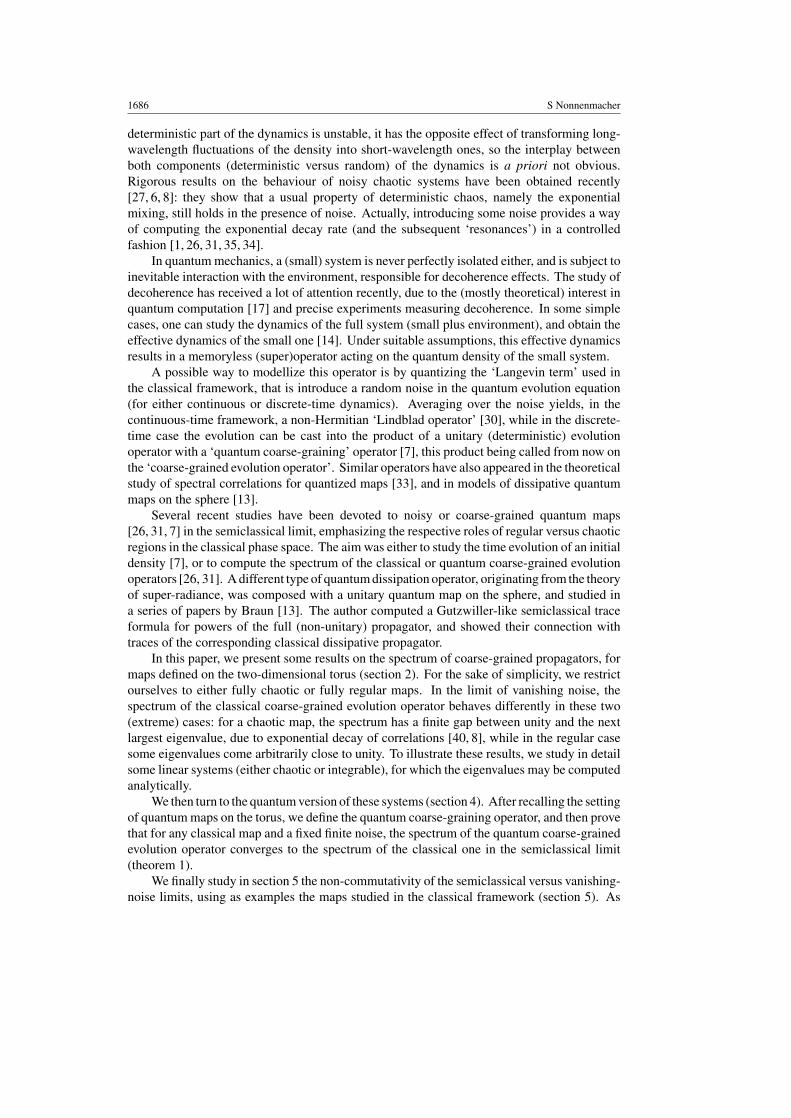
deterministic part of the dynamics is unstable, it has the opposite effect of transforming long-wavelength fluctuations of the density into short-wavelength ones, so the interplay betweenboth components (deterministic versus random) of the dynamics is a priori not obvious.Rigorous results on the behaviour of noisy chaotic systems have been obtained recently[27, 6, 8]: they show that a usual property of deterministic chaos, namely the exponentialmixing, still holds in the presence of noise. Actually, introducing some noise provides a wayof computing the exponential decay rate (and the subsequent ‘resonances’) in a controlledfashion [1, 26, 31, 35, 34].
In quantum mechanics, a (small) system is never perfectly isolated either, and is subject toinevitable interaction with the environment, responsible for decoherence effects. The study ofdecoherence has received a lot of attention recently, due to the (mostly theoretical) interest inquantum computation [17] and precise experiments measuring decoherence. In some simplecases, one can study the dynamics of the full system (small plus environment), and obtain theeffective dynamics of the small one [14]. Under suitable assumptions, this effective dynamicsresults in a memoryless (super)operator acting on the quantum density of the small system.
A possible way to modellize this operator is by quantizing the ‘Langevin term’ used inthe classical framework, that is introduce a random noise in the quantum evolution equation(for either continuous or discrete-time dynamics). Averaging over the noise yields, in thecontinuous-time framework, a non-Hermitian ‘Lindblad operator’ [30], while in the discrete-time case the evolution can be cast into the product of a unitary (deterministic) evolutionoperator with a ‘quantum coarse-graining’ operator [7], this product being called from now onthe ‘coarse-grained evolution operator’. Similar operators have also appeared in the theoreticalstudy of spectral correlations for quantized maps [33], and in models of dissipative quantummaps on the sphere [13].
Several recent studies have been devoted to noisy or coarse-grained quantum maps[26, 31, 7] in the semiclassical limit, emphasizing the respective roles of regular versus chaoticregions in the classical phase space. The aim was either to study the time evolution of an initialdensity [7], or to compute the spectrum of the classical or quantum coarse-grained evolutionoperators [26, 31]. A different type of quantum dissipation operator, originating from the theoryof super-radiance, was composed with a unitary quantum map on the sphere, and studied ina series of papers by Braun [13]. The author computed a Gutzwiller-like semiclassical traceformula for powers of the full (non-unitary) propagator, and showed their connection withtraces of the corresponding classical dissipative propagator.
In this paper, we present some results on the spectrum of coarse-grained propagators, formaps defined on the two-dimensional torus (section 2). For the sake of simplicity, we restrictourselves to either fully chaotic or fully regular maps. In the limit of vanishing noise, thespectrum of the classical coarse-grained evolution operator behaves differently in these two(extreme) cases: for a chaotic map, the spectrum has a finite gap between unity and the nextlargest eigenvalue, due to exponential decay of correlations [40, 8], while in the regular casesome eigenvalues come arbitrarily close to unity. To illustrate these results, we study in detailsome linear systems (either chaotic or integrable), for which the eigenvalues may be computedanalytically.
We then turn to the quantum version of these systems (section 4). After recalling the settingof quantum maps on the torus, we define the quantum coarse-graining operator, and then provethat for any classical map and a fixed finite noise, the spectrum of the quantum coarse-grainedevolution operator converges to the spectrum of the classical one in the semiclassical limit(theorem 1).
We finally study in section 5 the non-commutativity of the semiclassical versus vanishing-noise limits, using as examples the maps studied in the classical framework (section 5). As

Noisy classical and quantum propagators 1687
a byproduct, we show that one can obtain the resonances of a classical hyperbolic map fromthe spectrum of an associated quantum operator (the quantum coarse-grained propagator),provided the coarse-graining is set to decrease slowly enough in the semiclassical limit (weconjecture a sufficient condition for the speed of convergence). In contrast, for an integrablemap the same limit yields a spectrum densely filling one-dimensional curves (‘strings’) in theunit disc, one of them containing unity as a limit point.
2. Classical noisy evolution
The classical dynamical systems we will study are defined on a two-dimensional symplecticand Riemannian manifold, the torus T
2 = R2/Z
2. The maps are smooth (C∞), invertibleand leave the symplectic form dp ∧ dq (and therefore the volume element d2x = dq dp)invariant: they are canonical diffeomorphisms of T
2. Such a map x = (q, p) �→ Mx
naturally induces a Perron–Frobenius operator P = PM acting on phase space densitiesρ(x) : [Pρ](x) = ρ(M−1x).
2.1. Spectral properties of the classical propagator
In this section we review the spectral properties of the Perron–Frobenius operator PM ,depending on the map M and on the functional space on which the operator acts. The resultspresented are not new, but allow us to fix some notation.
2.1.1. Spectrum on L2(T2). For any canonical diffeomorphism M and any p � 1, thespectrum of PM on the Banach space Lp(T2) is a subset of the unit circle and admits ρ0(x) ≡ 1as invariant density. In particular, P is unitary on L2(T2) and on its subspace L2
0(T2) of
zero-mean densities.One can relate some dynamical properties of the map M with the (unitary) spectrum of P
on L20(T
2) [18]. For instance, if the dynamics M leaves invariant a non-constant observableH(x) ∈ C0(T2) (e.g. if M is the stroboscopic map of the Hamiltonian flow generated by H ),then all observables of the type ρ(x) = f (H(x)) (with f a smooth function) are invariant aswell, so that the eigenvalue 1 of P is infinitely degenerate. The full spectrum of P will beexplicitly given for some integrable maps in section 3.2.
In contrast, the map M is ergodic iff P has no invariant density in L20 (i.e. if 1 is a simple
eigenvalue in L2). Stronger chaotic properties may be defined in terms of the correlationfunction between two densities f, g ∈ L2:
Cfg(t)def=
∫T2
dx f (x)g(M−t x) = (f, P t g) (1)
(the time parameter t will always take integer values). The map M is said to be mixing iff forany f, g, the correlation function behaves for large times as:
Cfg(t)|t |→∞−→
∫T2
dx f (x)
∫T2
dx g(x). (2)
A slightly weaker property (weak mixing) is equivalent with the fact that PM has no eigenvaluein L2
0(T2).
2.1.2. Exponential mixing. For a certain class of maps (e.g. the Anosov maps definedlater), the convergence of mixing is exponentially fast, provided the observables f, g
are smooth enough. One speaks of exponential mixing with a decay rate γ > 0 if|Cfg(t)−
∫f dx
∫g dx| � Kfge−γ |t | for a certain constant Kfg .

1688 S Nonnenmacher
This behaviour can sometimes be explained through the spectral analysis of the Perron–Frobenius operator P acting on an ad hoc functional space B, with B �⊂ L2 (in generalB contains some distributions). One proves that the operator P on B is quasi-compact:its spectrum consists of finitely many isolated eigenvalues {λi} (called Ruelle–Pollicottresonances) situated in an annulus {r < λi < λ0 = 1} for some r > 0, plus a possibleessential spectrum inside the disc of radius r . In that case, assuming for simplicity that each λi
is a simple eigenvalue with spectral projector �i , the spectral decomposition of P on B leadsto the following asymptotic expansion for Cfg(t) in the limit t →∞:
Cfg(t) =∑
i
λti〈f, �ig〉 + O(rt ). (3)
In the above expression, the brackets do not refer to a Hermitian structure, but represent theintegrals
∫f (x)[�ig](x) dx. The first resonance λ0 = 1 corresponds to the unique invariant
density ρ0, and the decay rate (obviously independent of the observables f, g) is given byγ = − log |λ1|, respectively, by − log r if there is no resonance other than unity.
This type of spectrum was first put in evidence in the case of uniformly hyperbolic mapsby using Markov partitions to translate the dynamics on the phase space into a simple symbolicdynamics (namely a subshift of finite type) [40]. It was later extended to more general systems,including non-uniformly hyperbolic ones [4]. In the next sections, we will introduce theAnosov diffeomorphisms on the torus, which often serve as a ‘model’ for deterministic chaos.
2.1.3. Anosov diffeomorphism on the two-dimensional torus. In this section we recallthe definition and some properties of an Anosov diffeomorphism M on the torus T
2 [24].The Anosov property means that at each point x ∈ T
2, the tangent space TxT2 splits into
TxT2 = Es
x ⊕ Eux , where E
u/sx are the local stable and unstable subspaces. The tangent map
dxM sends Eu/sx to E
u/sM(x), and there exist constants A > 0, 0 < λs < 1 < λu (independent
on x) s.t.
∀t ∈ N, ‖(dxMt)|Es
x‖ � Aλt
s and ‖(dxM−t )|Eu
x‖ � Aλ−t
u . (4)
These inequalities describe the uniform hyperbolicity of M on T2. The splitting of TxT
2 intoE
u/sx has in general regularity C1+α for some 1 > α > 0, meaning that it is differentiable and
its derivatives are Holder-continuous with coefficient α.This uniform hyperbolicity implies that M is ergodic and exponentially mixing with
respect to the Lebesgue measure (see next section).Simple examples of Anosov diffeomorphisms are provided by the linear hyperbolic
automorphisms of T2, defined by matrices A ∈ SL(2, Z) with |trA| > 2. These maps
are sometimes referred to as ‘generalized cat maps’, in reference to Arnold’s ‘cat map’AArnold = (
2 11 1) [3]. We will study in some detail these linear maps and their quantizations,
and obtain a rather explicit description of the associated coarse-grained propagators. One canperturb the linear hyperbolic automorphism A with the stroboscopic map ϕ1
H generated bysome Hamiltonian H(x) on the torus: M
def= ϕ1H ◦ A. If the Hamiltonian H is ‘small enough’,
the perturbed map M remains Anosov, and topologically conjugated with the linear map A.
2.1.4. Ruelle resonances for Anosov diffeomorphisms. As announced above, Anosovdiffeomorphisms on T
2 are exponentially mixing, and their correlation functions satisfyexpansions of the type (3). Although the original proofs made use of Markov partitions [40],we will rather describe a more recent approach due to Blank et al [8], which has the advantageof providing spectral results for the coarse-grained propagator as well.

Noisy classical and quantum propagators 1689
The strategy of [8] is to define a Banach space B of densities on T2 adapted to the map
M: the space B contains distributions which are smooth along the unstable direction of M butpossibly singular (dual of smooth) along the stable direction. In particular, these functions aretoo singular to be in L2, which allows a non-unitary spectrum of P acting on B. The space B isdefined in terms of an arbitrary parameter 0 < β < 1, and satisfies the continuous one-to-oneembeddings: C1(T2)→ B → C1(T2)∗.
The space B depends on the map M , and also on the direction of time: the space BM−1
adapted to the map M−1 is different from BM . Although the map M on the torus is invertible,the dynamics of the operator P on the space B is irreversible: its spectrum is qualitatively verydifferent from that of P−1.
The authors indeed show that P is quasi-compact in B, with essential spectral radiusress bounded above by σ = max(λ−1
u , λβs ) (see equation (4) for the definition of λu/s). For
any 1 > r > σ , the spectrum of P in the ring Rrdef= {r � |λ| � 1} consists of isolated
eigenvalues, the Ruelle–Pollicott resonances {λi}. Therefore, a spectral expansion similarto (3) holds for any pair of observables f, g ∈ B, which includes in particular observablesin C1(T2) (the expansion might be slightly more complicated than (3) due to possible finitedegeneracies of the resonances).
A possible strategy to extend the results of [8] to maps and observables of regularity Ck
was discussed in the recent preprint [5]. Under stronger smoothness assumptions, namelyfor real-analytic Anosov maps in two dimensions, Rugh [41] constructed a transfer operatoracting on observables real-analytic along the unstable direction, and ‘dual of analytic’ alongthe stable one; he showed that this operator is compact, which means that the essential spectralradius vanishes in that case.
2.2. Coarse-grained classical propagator
In this section we precisely define the operator representing the effect of ‘noise’ on thedeterministic evolution of M . This operator is of diffusion type, it realizes a coarse-grainingof the densities.
2.2.1. Classical diffusion operator. We consider a smooth probability density K(x) on R2
with compact support. For simplicity, we also assume that K(x) = K(−x). From there, toany ε > 0 corresponds a probability density on the torus, defined as
Kε(x) = 1
ε2
∑n∈Z2
K(x + n
ε
).
Due to the compact support of K , we see that for small enough ε and any x ∈ T2 this sum
has at most one non-vanishing term (for x close to the origin). We define the coarse-grainingoperator Dε on L2(T2) as the following convolution:
∀f ∈ L2(T2), [Dεf ](y) =∫
T2dx Kε(y − x) f (x). (5)
Dε is a self-adjoint compact operator on L2(T2), with discrete spectrum accumulating at theorigin.
We define the Fourier transform on the plane as
K(ξ) =∫
R2dx K(x)e2iπξ∧x
with the wedge product given by ξ ∧ x = ξ1p− ξ2q. From the assumptions on the density K ,the function K(ξ) is real, even and smooth. It takes its maximum at ξ = 0 (where it behaves

1690 S Nonnenmacher
as K(ξ) = 1 −Q(ξ) + O(|ξ |4), with Q(·) a positive definite quadratic form), and decreasesfast for |ξ | → ∞.
The plane waves (or Fourier modes) on T2 are accordingly defined as ρk(x)
def=exp{2iπx ∧ k}, for k ∈ Z
2. They obviously form an orthonormal eigenbasis of the coarse-graining operator:
∀ε > 0, ∀k ∈ Z2, Dερk = K(εk)ρk. (6)
The fast decrease of the eigenvalues as |k| → ∞ implies that the operator Dε is not onlycompact, but also trace-class. It kills the small-wavelength modes, effectively truncating theFourier decomposition of ρ(x) at a cut-off |k| ∼ ε−1. For some instances, we will actuallyreplace the smooth function K(ξ) by a sharp cut-off �(1 − |ξ |) (with � the Heaviside stepfunction).
2.2.2. Classical coarse-grained propagator. The noisy dynamics associated with the map M
is represented by the product of the deterministic evolution PM with the diffusion operator:
PM,εdef= Dε ◦ PM. (7)
It may be more natural to define the noisy propagator as the more ‘symmetric’ Dε ◦PM ◦Dε , butboth definitions lead to the same spectral structure. PM,ε describes a Markov process definedby the deterministic map M followed by a random jump on a scale ε.
We now give some general properties of this operator, independent of the particular map M .Like the regularizing operator Dε , PM,ε maps distributions into smooth functions, and iscompact and trace-class on any functional space containing C∞(T2) as a dense subspace, witha spectrum independent of the space. Its eigenvalues {λµ,ε}µ�0 are inside the unit disc (onlyλ0,ε = 1 is exactly on the unit circle), they are of finite multiplicity and admit the origin as theonly accumulation point. The eigenvalue λ0,ε is simple, with unique eigenfunction ρ0. Pε mapsa real density to a real density, therefore its spectrum is symmetric with respect to the real axis.
In the next section we investigate in more detail the behaviour of these eigenvalues in thelimit of small noise, stressing the difference between chaotic versus regular maps.
3. Spectral properties of a classical coarse-grained propagator
We describe more precisely the spectrum of PM,ε , in the limit of small noise, and for differentclasses of maps M . We start with the most chaotic maps, namely the Anosov diffeomorphismsdefined in section 2.1.3, the exponential mixing of which was described in section 2.1.4. Inthe second part, we will then turn to the opposite case of ‘regular’ maps on T
2.
3.1. Anosov diffeomorphism
We use the same notation as in section 2.1.4 for M an Anosov map. It was proven in [8] thatthe spectrum of PM,ε outside some neighbourhood of the origin converges to the resonancespectrum of PM on the Banach space B.
More precisely, for M a smooth Anosov canonical diffeomorphism on T2 with foliations
of Holder regularity C1+α (0 < α < 1), one considers the ‘associated’ Banach space B = BM
defined in terms of a coefficient β < α, such that the essential radius of P on B has forupper bound σ = max(λ−1
u , λβs ). The authors then construct a ‘weak’ norm ‖ · ‖w on L(B),
such that ‖Pε − P‖w → 0 as ε → 0. As a consequence, for any 1 > r > σ , any λ
in the annulus Rr = {r � |λ| � 1} and any δ > 0 small enough, the spectral projector�
(ε)
B(λ,δ) of Pε (respectively, �B(λ,δ) of P) in the disc B(λ, δ) = {z : |z − λ| � δ} satisfies

Noisy classical and quantum propagators 1691
‖�(ε)
B(λ,δ)−�B(λ,δ)‖wε→0→ 0. Both projectors therefore have the same rank for ε small enough,
this rank being zero if the disc contains no resonance λi .This proves that the spectrum of Pε in the annulus Rr converges (with multiplicity) to the
set of resonances {λi} as ε → 0, and the eigenmodes of Pε weakly converge to correspondingeigenmodes of P (since the latter are genuine distributions, the convergence can only hold ina weak sense).
Remarks.
• These results also apply to the ‘symmetric’ coarse-graining Dε ◦ P ◦Dε .• It is reasonable to conjecture that these results hold as well if the coarse-graining kernel
K(x) is not compactly supported on R2, but decreases sufficiently fast, for instance if
one takes the Gaussian G(x)def= e−π |x|2 , G(ξ) = e−π |ξ |2 , as was done in [1, 26]. As a
broader generalization, we will sometimes consider a coarse-graining defined by a sharpcut-off in Fourier space, K(ξ) = �(1 − |ξ |), similar to the method used in [31]; afinite-rank coarse-graining was also used in [34] for one-dimensional noisy maps.
• If the map M and the kernel K(x) are real-analytic, we conjecture that the eigenvalues ofPε on any ring Rr with r > 0 converge to the resonances P in Rr (cf the remark at theend of section 2.1.4).
The (discrete) spectrum of Pε is the same on any space S admitting C∞ as dense subspace,in particular on L2, and this is the space we will consider from now on (more precisely,its subspace L2
0). This spectrum drastically differs from the absolutely continuous unitaryspectrum of the ‘pure’ propagator P on that space (cf section 2.1). The unitary spectrum isthus unstable upon the coarse-graining Dε : when switching on the noise, the spectral radiusof Pε on L2
0 suddenly collapses from 1 to |λ1| < 1. As we will see in the next sections,this collapse is characteristic of chaotic maps. We first describe it explicitly for the case ofhyperbolic linear automorphisms.
3.1.1. Example of Anosov maps: the hyperbolic linear automorphisms. In this section wereview [18, 27] the spectral analysis of the (pure versus noisy) propagator when the map A isa hyperbolic linear automorphism of T
2 (cf section 2.1.3). The unitary operator PA on L20 acts
very simply on the basis of Fourier modes ρk , k ∈ Z2∗ = Z
2\0, namely as a permutation:
[PAρk](x) = ρk(A−1x) = ρAk(x). (8)
This evolution induces orbits on the Fourier lattice Z2∗, which we will denote by O(k0) = {Atk0,
t ∈ Z}. Due to the hyperbolicity of A, each orbit is infinite, so that the modes {ρAtk0 , t ∈ Z}span an infinite-dimensional invariant subspace of L2
0, which we call Span O(k0). The spectralmeasure of PA associated with this subspace is of Lebesgue type (as usual when the operatoracts as a shift [39]). The number of distinct orbits being infinite, the spectrum of PA on L2
0 isLebesgue with infinite multiplicity.
Now we consider the coarse-grained propagator Pε,A = Dε ◦ PA. Since the ρk areeigenfunctions of Dε (cf equation (6)), Pε,A will also act as a permutation inside each orbitO(k0), but now at each step the mode ρk is multiplied by K(εk). Therefore, the operator Pε,A
restricted to the invariant subspace Span O(k0) can be represented as follows (the notation (·, ·)denotes the scalar product on L2
0):
Pε,A|O(k0) =∑t∈Z
K(εAt+1k0)(ρAtk0 , ·)ρAt+1k0 . (9)
Since |Atk0| → ∞ for t →±∞, the factors K(εAt+1k0) vanish in both limits. As a result, thespectrum of Pε,A|O(k0) reduces to the single point {0} (which is not an eigenvalue, but essential

1692 S Nonnenmacher
spectrum) [39]. By taking all orbits into account, the spectrum of Pε,A on L20 also reduces
to {0}: for linear hyperbolic maps, the collapse of the Lebesgue unitary spectrum throughcoarse-graining is ‘maximal’.
3.2. Coarse-graining of regular dynamics
In the previous sections we have considered classical propagators of Anosov diffeomorphismson T
2. We now describe the opposite case of an integrable map on T2. The notion of
integrability for a map is not so clear as for a Hamiltonian flow. In view of the examplesbelow, the definition should include the stroboscopic map MH = ϕ1
H of the flow generatedby an autonomous Hamiltonian H(x) on T
2, but it should also encompass elliptic andparabolic automorphisms, as well as rational translations. A required property is that thephase space T
2 splits into a union of invariant one-dimensional (not necessarily connected)closed submanifolds, with possible ‘critical energies’. Note that this condition excludes the(un)stable manifolds of an Anosov map, which are open. A more or less equivalent condition forintegrability is that the map leaves invariant a nowhere constant smooth function H(x), the levelcurves of which provide the above submanifolds. As a result, any density ρ(x) = f (H(x)) isinvariant through PM as well, so that PM has an infinite-dimensional eigenspace of invariantdensities on L2
0 (which we will call Vinv).The rest of the spectrum of PM can be of various types, as we will see (it can be pure point
or absolutely continuous, be a mixture, etc). For this reason, a general statement concerningthe coarse-grained spectrum of these maps cannot be very precise.
In the following sections we consider some simple examples of integrable maps for which(part of) the spectrum can be analysed in detail. We then discuss (mostly by hand-waving) thegeneral case.
3.2.1. Translations on the torus. The simplest nontrivial maps on T2 are the translations
x �→ Tvx = x +v mod T2, which do not derive from a Hamiltonian on the torus. A translation
is either ergodic (yet non-mixing) or integrable (see later).The spectrum of the corresponding Perron–Frobenius operator Pv = PTv
on L20 is easy to
describe [18]: Pv admits the Fourier modes ρk as eigenstates, with eigenvalues e2iπk∧v . Thespectrum of Pv is therefore pure point, with possible degeneracies. The spectrum of the coarse-grained propagator Pε,v = Dε ◦ Pv on L2
0 is also easy to describe: each Fourier mode ρk is aneigenfunction with eigenvalue K(εk)e2iπk∧v inside the unit disc. From the small-ε expansionK(εk) ∼ 1−ε2Q(k), the eigenvalues corresponding to long wavelengths (|k| � ε−1) are closeto the unit circle for small ε, while the short wavelength eigenvalues (|k| � ε−1) accumulatenear the origin. We now describe how the global aspect of the spectrum qualitatively dependson the translation vector v.
• Tv is ergodic iff the coefficients v1, v2 as well as their ratio v1/v2 are irrational: in thatcase, the equation k ∧ v ∈ Z has no solution for k �= 0. The spectrum of Pv forms adense subgroup of the unit circle, all eigenvalues being simple. In the limit ε → 0+, thespectrum of Pε,v becomes ‘dense’ in the unit disc (a similar quantum spectrum is plottedin figure 4, right).
• If one of the coefficients v1, v2, v1/v2 is rational, Tv leaves invariant a family of parallelone-dimensional ‘affine’ submanifolds, and is therefore integrable according to ourdefinition. For instance, if we take v1 = r/s (with r, s coprime integers) and v2 irrational,then for any q0 ∈ [0, 1], the union of vertical lines
⋃s−1l=0 {q = q0 + l/s} is invariant (if
s > 1, this set is non-connected). The spectrum of Pv is still dense on the circle, but all
Noisy classical and quantum propagators 1693
eigenvalues are now infinitely degenerate: for any k0, the modes k = k0 + (0, js), j ∈ Z
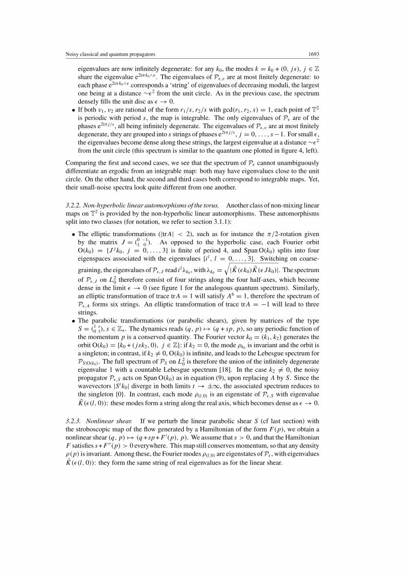
share the eigenvalue e2iπk0∧v . The eigenvalues of Pε,v are at most finitely degenerate: toeach phase e2iπk0∧v corresponds a ‘string’ of eigenvalues of decreasing moduli, the largestone being at a distance ∼ε2 from the unit circle. As in the previous case, the spectrumdensely fills the unit disc as ε → 0.
• If both v1, v2 are rational of the form r1/s, r2/s with gcd(r1, r2, s) = 1, each point of T2
is periodic with period s, the map is integrable. The only eigenvalues of Pv are of thephases e2iπj/s , all being infinitely degenerate. The eigenvalues of Pε,v are at most finitelydegenerate, they are grouped into s strings of phases e2iπj/s , j = 0, . . . , s−1. For small ε,the eigenvalues become dense along these strings, the largest eigenvalue at a distance∼ε2
from the unit circle (this spectrum is similar to the quantum one plotted in figure 4, left).
Comparing the first and second cases, we see that the spectrum of Pε cannot unambiguouslydifferentiate an ergodic from an integrable map: both may have eigenvalues close to the unitcircle. On the other hand, the second and third cases both correspond to integrable maps. Yet,their small-noise spectra look quite different from one another.
3.2.2. Non-hyperbolic linear automorphisms of the torus. Another class of non-mixing linearmaps on T
2 is provided by the non-hyperbolic linear automorphisms. These automorphismssplit into two classes (for notation, we refer to section 3.1.1):
• The elliptic transformations (|trA| < 2), such as for instance the π/2-rotation givenby the matrix J = (
0 −11 0 ). As opposed to the hyperbolic case, each Fourier orbit
O(k0) = {J jk0, j = 0, . . . , 3} is finite of period 4, and Span O(k0) splits into foureigenspaces associated with the eigenvalues {il, l = 0, . . . , 3}. Switching on coarse-
graining, the eigenvalues of Pε,J read ilλk0 , with λk0 =√|K(εk0)K(εJ k0)|. The spectrum
of Pε,J on L20 therefore consist of four strings along the four half-axes, which become
dense in the limit ε → 0 (see figure 1 for the analogous quantum spectrum). Similarly,an elliptic transformation of trace trA = 1 will satisfy A6 = 1, therefore the spectrum ofPε,A forms six strings. An elliptic transformation of trace trA = −1 will lead to threestrings.
• The parabolic transformations (or parabolic shears), given by matrices of the typeS = (
1 s0 1), s ∈ Z∗. The dynamics reads (q, p) �→ (q + sp, p), so any periodic function of
the momentum p is a conserved quantity. The Fourier vector k0 = (k1, k2) generates theorbit O(k0) = {k0 + (jsk2, 0), j ∈ Z}: if k2 = 0, the mode ρk0 is invariant and the orbit isa singleton; in contrast, if k2 �= 0, O(k0) is infinite, and leads to the Lebesgue spectrum forPS|O(k0). The full spectrum of PS on L2
0 is therefore the union of the infinitely degenerateeigenvalue 1 with a countable Lebesgue spectrum [18]. In the case k2 �= 0, the noisypropagator Pε,S acts on Span O(k0) as in equation (9), upon replacing A by S. Since thewavevectors |Stk0| diverge in both limits t → ±∞, the associated spectrum reduces tothe singleton {0}. In contrast, each mode ρ(l,0) is an eigenstate of Pε,S with eigenvalueK(ε(l, 0)): these modes form a string along the real axis, which becomes dense as ε → 0.
3.2.3. Nonlinear shear. If we perturb the linear parabolic shear S (cf last section) withthe stroboscopic map of the flow generated by a Hamiltonian of the form F(p), we obtain anonlinear shear (q, p) �→ (q +sp+F ′(p), p). We assume that s > 0, and that the HamiltonianF satisfies s+F ′′(p) > 0 everywhere. This map still conserves momentum, so that any densityρ(p) is invariant. Among these, the Fourier modes ρ(l,0) are eigenstates of Pε , with eigenvaluesK(ε(l, 0)): they form the same string of real eigenvalues as for the linear shear.

1694 S Nonnenmacher
For any n ∈ Z∗, P and Pε leave invariant the subspace Vn = Span {e2iπnqρ(p),ρ ∈ L2(T1)}, and their spectra on this subspace can be partially described, at least if one takesF ′ small enough and replaces the kernel K(ξ) by the sharp cut-off �(1 − |ξ1|)�(1 − |ξ2|)(such that Dε projects to a finite-dimensional subspace). The spectrum of P on Vn is absolutelycontinuous, while that of Pε is contained in a small neighbourhood of the origin, uniformlywith respect to n and ε (see appendix A.1 for details). The spectrum should be qualitatively thesame if K(ξ) is of fast decrease at infinity.
3.2.4. Stroboscopic map of the Harper Hamiltonian flow. As a last example of an integrablemap, we consider the Harper Hamiltonian on the torus
H(x) = cos(q) + cos(p) = 12 (ρ(1,0) + ρ(−1,0) + ρ(0,1) + ρ(0,−1))
and take its stroboscopic map M = ϕ1H . The invariant densities are of the form ρ(x) =
f (H(x)). As opposed to what happened for the parabolic shear, Vinv is not invariant throughthe diffusion operator Dε , so the spectrum of Pε is more complicated to analyse. Still, ifwe take a coarse-graining kernel satisfying K(ξ) = k(|ξ1| + |ξ2|) along the axes of slopes0,± 1
2 , ±1, ±2, ∞ then the invariant functions H(x), (H(x))2 − 1 and (H(x))3 − 94H(x)
are eigenstates of Dε and therefore of Pε , with respective eigenvalues k(ε), k(2ε) and k(3ε)
(if the kernel only satisfies K((0, ζ )) = K((ζ, 0)) together with even parity, then H(x) willbe an eigenstate of Pε with eigenvalue K((ε, 0))). These eigenvalues are real and approachunity as ε → 0. Numerically, they are the first three elements (respectively, the first element)of a string of real eigenvalues connecting unity to the origin, the further elements of the stringbeing mixtures of invariant and non-invariant densities (see figure 5, right, for a similar quantumspectrum).
3.2.5. General behaviour for an integrable map. After these examples, we want to describethe spectrum of PM,ε for M an integrable map, say the stroboscopic map of an autonomousHamiltonian H . As we already explained, the space Vinv of invariant densities is infinite-dimensional, containing all densities f (H(x)). When applying the coarse-graining Dε , onegenerally mixes these invariant densities with non-invariant ones (as opposed to what happensfor the linear maps described above). Using ideas of degenerate perturbation theory, weconjecture the following behaviour, which is supported by numerical investigations [31, 26].
The invariant subspace Vinv contains modes ρlw with long-wavelength fluctuations (i.e.densities for which the Fourier spectrum is concentrated in a finite region near k = 0). For ε
small, these modes are hardly modified by the coarse-graining operator: Dερlw−ρlw = O(ε2).This suggests that Pε has an eigenstate of the type ρlw + O(ε2), of eigenvalue 1− O(ε2), thiseigenstate being close to an invariant state of P . In contrast, Vinv also contains highly fluctuatingmodes, which will be very damped by Dε , and should lead to eigenstates of Pε close to theorigin. As a whole, the hybridization of invariant modes with non-invariant ones leads to astring of eigenvalues connecting unity to the origin, this string being symmetrical with respectto the real axis. Note that the projected operator �invPε�inv = �invDε�inv = (where �inv
is the orthogonal projector on the space Vinv) is self-adjoint, therefore its spectrum can beestimated through the min–max method: for ε → 0 it consists in a dense string of eigenvaluesbetween unity and zero. I believe that the largest eigenstates (-values) of this projected operatorare close to eigenstates (-values) of Pε .
Conclusion: qualitatively different spectra. We have exhibited a qualitative difference of thecoarse-grained Perron–Frobenius spectra between, on the one hand, the chaotic maps (Anosov),and on the other hand, non-mixing maps, including ergodic translations and integrable maps.

Noisy classical and quantum propagators 1695
In the latter case, the spectrum of Pε on the subspace L20(T
2) comes close to the unitcircle for small ε, either along one-dimensional strings ‘connecting’ the origin to infinitelydegenerate eigenvalues of P (among which unity), or by densely filling the unit disc (for ergodictranslations). A common feature is that any annulus {R < |λ| < 1} (or any open neighbourhoodof unity) contains more and more eigenvalues of Pε in the small-noise limit ε → 0.
In contrast, for an Anosov map the spectrum of Pε on L20 is contained inside a disc of radius
R < 1, uniformly for small enough ε. This spectrum consists in a finite number (possiblyzero) of finitely degenerate eigenvalues (asymptotically close to the Ruelle resonances) insidean annulus {r < |λµ,ε | � R}, the remaining eigenvalues having moduli smaller than r .
The numerical results of [31, 26] go beyond this statement: the authors consider systemswith mixed dynamics (not to be mistaken with the ‘mixing’ property of Anosov maps), thatis systems for which the phase space splits into ‘regular islands’ embedded in a ‘chaotic sea’.They study the spectrum of the coarse-grained Perron–Frobenius operator (the coarse-grainingis taken as a cut-off in Fourier space), and show the presence of eigenvalues close to the unitcircle, the eigendensities of which are supported on the regular islands; on the other hand, theyalso find some eigenvalues inside the unit circle, which are associated with the chaotic part ofphase space, and therefore interpreted as (generalized) Ruelle resonances. Yet, the nature ofthe ‘chaotic sea’ in such systems is not well understood at the mathematical level, so that arigorous spectral analysis of the propagator seems a quite distant goal.
4. Quantum coarse-grained evolution
After studying the effect of noise on classical propagators, we turn to noisy quantum maps,obtained by quantizing the classical ones. Although we will restrict ourselves to maps on the2-torus, the main result of this section (theorem 1) can be straightforwardly generalized toquantum maps on any compact phase space, provided one adapts the definition of the coarse-graining operator (see the discussion in section 4.2.3). We start by recalling the setting ofquantized maps on the 2-torus.
4.1. Quantum propagator on the torus
4.1.1. Quantum Hilbert space and observables. We briefly review the construction ofquantum mechanics on T
2, in order to fix notation. For any value of h > 0, the Weyl–Heisenberg group associates with each vector v = (v1, v2) ∈ R
2 the ‘quantum translation’Tv = exp{(i/h)(v2q − v1p)} which acts unitarily on L2(R). These translations satisfy thegroup relations TvTv′ = e−(i/2h)v∧v′ Tv+v′ .
The ‘torus wavefunctions’ are then defined as distributions |ψ〉 ∈ S ′(R) satisfyingthe periodicity conditions T(0,1)|ψ〉 = T(1,0)|ψ〉 = |ψ〉. Due to the group relations, suchdistributions exist iff h satisfies the condition (2πh)−1 = N ∈ N (such a value of h will becalled admissible). In that case they form a space of dimension N , which will be denotedHN [23]. A basis of this space is provided by the ‘Dirac combs’ {|qj 〉N }j=0,...,N−1 defined as:
〈q|qj 〉N =∑ν∈Z
δ(q − qj − ν), with qj = j
N. (10)
By construction, |qj 〉N = |qj+N 〉N , so the index j must be understood modulo N .For practical reasons, we will choose the following representatives of integers moduloN : ZN = {−N/2 + 1, . . . , N/2} for N even, ZN = {−(N − 1)/2 + 1, . . . , (N − 1)/2} forN odd.

1696 S Nonnenmacher
The quantum translation Tv acts inside HN iff v is on the square lattice of side 1/N , thatis v = (V1/N, V2/N) with Vi ∈ Z. Besides, each translation with integer coefficients actson HN as a multiple of the identity. As a result, the set {TV/N , V ∈ Z
2N } forms a basis of
the space of linear operators on HN , denoted by L(HN). This basis can be used to definethe Weyl quantization of smooth observables f ∈ C∞(T2). From the Fourier decompositionf =∑
k∈Z2 f (k)ρk , the Weyl quantization of the observable f is defined as
f = OpN(f )def=
∑k∈Z2
f (k)Tk/N =∑k∈Z
2N
Tk/N
(∑ν∈Z2
(−1)Nν1ν2+k∧ν f (k + Nν)
). (11)
The ‘converse’ of Weyl quantization, that is the Weyl symbol (or Wigner function) WB(x) of anoperator B ∈ L(HN) is also easily defined through its Fourier transform: for each k ∈ Z
2, itsFourier coefficient WB(k) is given by WB(k) = (1/N)tr(T †
k/N B). These Fourier coefficientsare N -periodic (up to a sign), so that the ‘function’ WB(x) is a periodic combination of Diracpeaks on the lattice of side 1/2N [23]. Alternatively, a polynomial Weyl symbol was definedin [19] as the finite sum
WP
B(x) =
∑k∈Z
2N
WB(k)e2iπx∧k.
As opposed to the former symbol, the polynomial symbol depends on the specific choicefor the representative ZN (the choice we made, with maximum symmetry around the origin,seems more natural in this respect). The polynomial symbol map together with OpN yield anisometric isomorphism between the subspace IN
def= Span {ρk , k ∈ Z2N } of L2(T2) and the
space of observables on HN equipped with the Hilbert–Schmidt scalar product (B, C) =(1/N)tr(B†C). Since the Hilbert–Schmidt norm differs from the usual operator norm onL(HN), we will denote by L2
N the space of observables on HN (i.e. N ×N matrices) equippedwith the Hilbert–Schmidt norm.
4.1.2. Quantization of canonical maps. We briefly explain how one quantizes a canonicalmap M on T
2. The aim is to define for each N ∈ N a unitary operator on HN (which we willdenote by MN or simply M) which satisfies prescribed semiclassical properties [42]. Theseproperties do not unambiguously define the sequence of unitary matrices, so a choice has to bemade (in [44], a Toeplitz quantization is proposed for symplectic maps on Kahler manifolds).We present here another quantization prescription, which uses the following decomposition ofany canonical map M on T
2 [16]:
M = A ◦ Tv ◦ ϕ1H . (12)
In this formula, the linear automorphism A ∈ SL(2, Z) and the translation Tv are uniquelydefined. In contrast, the last factor corresponds to the stroboscopic map of the flow of atime-dependent periodic Hamiltonian H ∈ C∞(T2
x × Tt ); this Hamiltonian is not unique,since two Hamiltonians H1 �= H2 may lead to the same stroboscopic map ϕ1
H1= ϕ1
H2. From
this decomposition, one can quantize M as follows [25]. First, one quantizes a la Weyl theHamiltonian H(x, t) into the operator H (t) on HN , then take for the quantization of ϕ1
H thetime-ordered exponential T e−i
∫ 10 dt H (t)/h. Second, one may quantize the translation Tv with
the quantum translation Tv(N) , where the vector v(N) belongs to the 1/N -lattice and is close tov, for instance take
v(N) = ([Nv1], [Nv2])
N
[32]. Third, provided A satisfies the condition A ≡ Id2 mod 2 or A ≡ σx mod 2, the linearautomorphism A is ‘naturally’ quantized into a unitary matrix AN [23] (this condition may

Noisy classical and quantum propagators 1697
be relaxed if one generalizes the quantum Hilbert space HN to arbitrary ‘Bloch angles’ [12]).Finally, the map M is quantized on HN as the product:
MN = AN ◦ Tv(N) ◦ T e−i2πN∫ 1
0 dt H (t). (13)
This choice for the quantum map automatically satisfies the Egorov property [12,32]: for anyclassical observable ρ ∈ C∞(T2),
MN OpN(ρ)M−1N −OpN(ρ ◦M−1)
N→∞−→ 0. (14)
This means that the quantization and finite-time evolution of densities commute in thesemiclassical limit (the convergence holds for the operator norm in L(HN)).
In practice, the classical maps we consider are all defined as products of automorphisms,translations and Hamiltonian maps, so they admit a ‘natural’ quantization.
4.1.3. Propagator of quantum densities. The quantum map M propagates quantum states|ψ〉 ∈ HN . A density matrix ρ is an element of the space L2
N = HN ⊗H∗N , and its evolution
through the quantum map reads ρ �→ MρM−1 = ad(M)ρ. The operator PMdef= ad(M)
acting on the space L2N is the quantum analogue of the Perron–Frobenius operator PM acting
on classical densities. PM is unitary, with eigenvalues {ei(θj−θi ); i, j = 1, . . . , N}, where{eiθj } are the eigenvalues of the matrix M . In contrast with its classical analogue, the spaceof invariant densities through PM is at least N -dimensional, since it contains all the rank-1projectors |φi〉〈φi |, where |φi〉 are the eigenstates of M .
The operator P acting on densities is called a super-operator, to contrast with an operatoracting on HN . Being the adjoint action of a unitary matrix, it conserves the purity of the density,which means that a pure density ρ = |ψ〉〈ψ | is mapped onto a pure density Pρ = |ψ ′〉〈ψ ′|.We notice that P conserves the trace of the density, that is the quantum counterpart of the totalprobability of the density ρ.
4.2. Quantum coarse-graining operator
As we remarked above, the spectrum of P on L2N is qualitatively different from that of P on
L2(T2): the former has at least N invariant eigenstates, while the latter may have only one ifthe map M is ergodic. In section 2.1, we explained how the spectrum of P was sensitive to thefunctional space on which P acts. This is no longer the case in the quantum framework, sincethe propagator is a finite-dimensional matrix. Still, we showed in section 3 an alternative wayto obtain the (non-unitary) resonance spectrum of an Anosov map, namely by introducing somenoise and studying the spectrum of the noisy propagator Pε = Dε ◦ P on the space L2(T2).This procedure can also be carried out at the quantum level, by first defining a ‘quantumcoarse-graining’ or ‘quantum diffusion’ (super)operator Dε , using it to construct a quantumcoarse-grained propagator Pε , then studying the spectrum of the latter on L2
N . To connect theclassical and quantum frameworks, we will consider the semiclassical limit N →∞.
4.2.1. Definition. We define the coarse-graining superoperator by analogy with the classicalone (equation (5)). The latter can be expressed as follows:
∀f ∈ L2(T2), (Dεf )(x) =∫
T2dv Kε(v)ρ(x − v) =
∫T2
dv Kε(v)(Pvρ)(x) (15)
where Pv is the Perron–Frobenius operator for the translation Tv . Since Tv is quantized on HN
into the unitary matrix Tv(N) , a natural way to define a quantum coarse-graining super-operator

1698 S Nonnenmacher
would be through the integral∫T2
dv Kε(v)Pv(N) .
For convenience, we prefer a slightly different definition. The map v �→ v(N) is constant onsquares of side 1/N , so the above integral reduces to a finite sum over V ∈ Z
2N , with each
operator PV/N multiplied by the average of Kε over the corresponding square. Kε being asmooth function, this average is semiclassically close to the value Kε(V/N), therefore for N
large the above integral is well approximated by the sum:
Dε = F(ε, N)
N2
∑V∈Z
2N
Kε
(V
N
)ad(TV/N). (16)
The prefactor F(ε, N) is needed to guarantee that Dε conserves the trace, that is Dερ0 = ρ0.This factor is easily expressed in terms of the two-dimensional theta function:
θK(εN, ζ )def=
∑ν∈Z2
K(εN(ν + ζ )), ζ ∈ T2. (17)
For Gaussian coarse-graining K(x) = G(x) = e−π |x|2 , this function reduces to the product oftwo classical Jacobi one-dimensional theta functions. In the limit εN � 1, the function θK ispeaked around the point ζ = 0, due to the fast decrease of K(ξ). Now, one easily checks thatF(ε, N) = θK(εN, 0)−1 converges to K(0) = 1 in the limit εN →∞.
4.2.2. Spectrum of the quantum coarse-graining operator. The spectrum of Dε on L2N is as
easy to analyse as that of Dε (see equation (6)). Using the group relation
ad(Tv)Tv′ = e−i(v∧v′/h)Tv′ (18)
we see that for any k ∈ Z2N , the quantum translation Tk/N (=OpN(ρk)) is an eigenstate of Dε
with eigenvalue
d(N)ε,k =
F(ε, N)
N2
∑V∈Z
2N
Kε
(V
N
)e2iπk∧(V/N) = θK(εN, k/N)
θK(εN, 0). (19)
For fixed k and εN →∞, one has the asymptotics d(N)ε,k = K(εk) + O((εN)−α) for any power
α > 0, so that the eigenvalue of Dε associated with Tk/N converges to the eigenvalue of Dε
associated with its symbol ρk . The estimate is sharper in the Gaussian case:
∀k ∈ Z2N, d
(N)ε,k = e−πε2k2
+ O(e−π(εN)2/4) (20)
so that the relative deviations between classical and quantum eigenvalues are exponentiallysmall, uniformly on the modes k ∈ {|k1|, |k2| � (N/2)(1 − δ)} (with δ > 0 fixed). For theGaussian case, both classical and quantum spectra are strictly positive, which is not true ingeneral. The spectrum of Dε for a Gaussian noise is plotted in figure 1 (left).
If we replace K(ξ) by the sharp cut-off �(1−|ξ |), then d(N)ε,k = 1 for |k| < ε−1, d(N)
ε,k = 0otherwise: the coarse-graining truncates the expansion (11), keeping only short wavevectors(modulo N ). In other words, Dε truncates the Fourier series of the polynomial Weyl symbolWP
ρ, keeping only the coefficients |k| < ε−1.A Fourier cut-off was also used as a definition for the quantum coarse-graining in [31],
but there the cut-off was applied to the Husimi function of ρ instead of its polynomial Weylsymbol.

Noisy classical and quantum propagators 1699
4.2.3. Probabilistic interpretation and generalizations of coarse-graining. In a differentphysical framework (one-dimensional quantum spin chains), Prosen [38] recently defined asimilar quantum coarse-graining by truncating the densities on finite-dimensional spaces. Inthis case, the quantum densities are decomposed into sums of spin operators acting on finitesequences of spins (e.g. σ1(x)σ1(x + 1) · · · σ1(x + l)). The truncation consists in keeping onlythose operators for which l � ε−1.
The right-hand side of equation (16) expresses the super-operator Dε in the Krausrepresentation, i.e. as a sum
∑j ad(Ej ), where the operators Ej on HN satisfy the condition∑
j E†j Ej = IdN . Kraus super-operators conserve the trace and the ‘complete positivity’ of
density matrices [17].The right-hand side of equations (15) and (16) may be interpreted as a random global jump
for the density, which jumps at a distance v with a probability ∝Kε(v). Dερ and its quantumcounterpart represent the average over all these random jumps. Since Dε or Dε do not dependon time, they therefore represent the classical and quantum versions of a memoryless Markovprocess.
In a different scope, a super-operator similar to Dε was used in [33] to study the spectralcorrelations of the quantum map M in the semiclassical limit. Coarse-graining was thereinterpreted as an average over a set of quantum maps close to identity. The phase space canbe an arbitrary (quantizable) symplectic manifold, and the classical and quantum averages aregenerated by a finite set of Hamiltonians {Hj }j=1,...,f ; Kε is a smooth probability kernel inf variables with compact support of scale ε around the origin. The classical and quantumcoarse-graining operators are defined as:
D{Hj }ε ρ(x) =
∫R
df t Kε(t)ρ(ϕ−1∑
j tj Hj(x)
),
D{Hj }ε ρ =
∫Rf
df t Kε(t)ad(e−i
∑j Hj tj /h
)ρ.
(21)
This scheme is more general than what we have done on the torus: one does not need anygroup action on the phase space, but only a sufficient number of Hamiltonians. We recoverour previous definition on the torus if we take for ‘Hamiltonians’ the multivalued functionsH1 = p mod 1, H2 = −q mod 1 (these functions are not well defined on T
2, but their flowsare). The qualitative spectral features of the classical coarse-grained propagator D
{Hj }ε for small
ε should not depend on the selected family of Hamiltonians {Hj }, as long as the second-orderoperator
∑f
j=1(∇Hj)2 is elliptic (in the above case on the torus, this is the Laplace operator
∂2/∂q2 + ∂2/∂p2, which is indeed elliptic) [27].In the framework of quantum mechanics on the 2-sphere, a different type of dissipative
super-operator Pτ = Dτ ◦ ad(M) was considered in [13], where Dτ is a quantum dissipationoperator obtained by integrating a quantum master equation during the time τ . Thisdissipation operator first appeared in the study of super-radiance in atomic physics [10]. Asa main difference with our noisy propagator Pε , the (unique) invariant eigenmode of Pτ isdifferent from ρ0. This corresponds to the fact that the corresponding classical propagatorPτ (obtained from Pτ by taking the semiclassical limit) does not leave invariant the uniformdensity ρ0, but rather a more singular measure, which may be supported either on a discreteset of points, or even on a more complicated ‘strange attractor’.
4.3. Quantum coarse-grained propagator
We will now study the quantum analogue of Pε , that is the coarse-grained quantum propagatorPε = Dε ◦ PM . Similarly as the classical propagator, Pε maps a Hermitian density to a

1700 S Nonnenmacher
Hermitian density; as a result, its spectrum is symmetric with respect to the real axis. Like Dε ,Pε is a Kraus super-operator, and therefore realizes a quantum Markov process: the quantumdensity first evolves through the deterministic map ad(M), then performs a random quantumjump through ad(TV/N), with a probability ∝Kε(V/N).
Linear combinations of quantum translations were considered in [7] as models fordecoherence on the quantum torus. The authors studied the evolution of densities through anoperator similar to Pε , by computing the time evolution of the ‘purity’ tr(ρ2). They took for M
the quantized baker’s map, which is fully chaotic, yet discontinuous on T2. More recently,
similar computations were performed for smooth nonlinear perturbations of cat maps [21].The author of [13] uses Gutzwiller-type trace formulae to estimate the traces of powers
of the dissipative quantum propagator tr(Pnτ ), in the regime of n fixed and h → ∞; from
them he shows that each trace converges to the corresponding trace of the classical dissipativepropagator tr(Pn
τ ) (this trace being given by a sum over periodic orbits as well).In the following I will not use any trace formula, but more basic semiclassical and operator-
theoretic techniques to compare quantum and classical coarse-grained propagators. Pε isindeed spectrally similar to its classical counterpart Pε . It conserves the trace: Pε ρ0 = ρ0,but in contrast with its noiseless version P , it has for unique invariant density ρ0, all othereigenvalues (in number N2 − 1) being inside the unit disc. As a non-classical property, Pε
destroys purity: the image of a pure state ρ = |ψ〉〈ψ | is not a pure state.The following theorem, which is the central result of this paper, relates more precisely the
spectra of Pε and Pε in the semiclassical limit: it states the ‘semiclassical spectral stability’ ofcoarse-grained propagators.
Theorem 1. For any smooth map M on the torus and any fixed ε > 0, the spectrum of thequantum coarse-grained propagator Pε = Dε ◦ PM on L2
N converges in the semiclassicallimit N →∞ to the spectrum of the classical coarse-grained propagator Pε = Dε ◦ PM onL2(T2). For any r > 0, the convergence is uniform in the annulus Rr = {r � |λ| � 1}.
To compare the classical and quantum propagators, we use the isometry between thesubspace IN of L2(T2) and L2
N , induced by the Weyl quantization OpN and its inverse WP
(see section 4.1.1 for notation). Pε is then isometric to σN(Pε)def= WP ◦ Pε ◦OpN ◦�IN
(�IN
projects orthogonally L2(T2) onto IN ). We therefore need to compare the operators σN(Pε)
and Pε on L2(T2). The crucial semiclassical estimate is the following lemma.
Lemma 1. The finite-rank operators σN(Pε) converge to Pε in the operator norm on L2(T2),in the limit N →∞.
Proof. The key semiclassical ingredient is Egorov’s property (14). From the norm inequality
‖ρ‖2HS =
1
Ntr(ρ†ρ) � ‖ρ‖2
L(HN ),
the convergence in (14) also holds for the Hilbert–Schmidt norm, that is on the space L2N .
Using the symbol map WP and its inverse OpN on IN , we will convert operators on L2N into
operators on L2(T2). We notice that for any k ∈ Z2, ρk ∈ IN for large enough N . The evolved
density PMρk is in general not in IN , but it is smooth since M is so. Any smooth density ρ isasymptotically equal to its projection on IN , so that
∀ρ ∈ C∞(T2), ‖WP ◦OpN(ρ)− ρ‖L2(T2)
N→∞−→ 0.
Using this fact, Egorov’s property can be recast into:
∀k ∈ Z2, ‖σN(PM)ρk − PMρk‖L2(T2)
N→∞−→ 0.

Noisy classical and quantum propagators 1701
This means that the sequence of operators σN(PM) semiclassically converges to PM in thestrong topology on B(L2) (the bounded operators on L2(T2)). Now, a standard lemma infunctional analysis [11, lemma 2.8] states that if a sequence An of bounded operators on someBanach space converges strongly to the operator A, then for any compact operator K , KAn
converges to KA in the operator norm. Since Dε is compact, this implies that Dε ◦ σN(PM)
converges to Pε,M in the operator norm. A simple comparison of the eigenvalues shows that‖σN(Dε)−Dε‖B(L2) → 0 as N →∞, which achieves the proof of the lemma. �
End of proof of the theorem. From lemma 1, one applies standard methods to show thatthe spectrum of σN(Pε) converges to that of Pε , as was done in section 3.1. Namely, for anyλ �= 0 and any small disc B(λ, δ) around it, the spectral projectors for σN(Pε) and Pε in thatdisc satisfy ‖�(N)
B(λ,δ) −�B(λ,δ)‖ → 0 as N →∞. For small enough δ, the projector �B(λ,δ)
is independent of δ and of finite rank, equal to the multiplicity of λ in the spectrum of Pε . Theabove convergence implies that �
(N)
B(λ,δ) has the same rank for N large enough, and that thecorresponding eigenspaces of Pε and σN(Pε) are close to each other. Finally, the spectrum ofPε is identical with that of σN(Pε). �
This spectral stability was noticed numerically in [31] for the kicked rotator on the2-sphere. In their case, the coarse-graining consists in a sharp truncation of the Fourierexpansion of the Husimi functions of the quantum densities, but the same arguments asabove can be applied to show the spectral stability of the coarse-grained propagator in thesemiclassical limit.
5. On the non-commutativity of the semiclassical versus small-noise limits
In the previous section we have described the semiclassical limit of the quantum coarse-grainedpropagator Pε for a fixed coarse-graining width ε > 0. On the other hand, section 3 was dealingwith the small-noise limit ε → 0 for the classical propagator Pε .
These two limits do not commute. Indeed, for fixed N ∈ N the coarse-graining operator Dε
is a finite matrix, the N2 eigenvalues of which converge to unity as ε → 0 (see equation (19)).Therefore, in this limit ‖Dε − IdL2
N‖ → 0. For K(x) of compact support, we even have
Dε = IdL2N
as soon as the rescaled support (εN)Supp(K) has no intersection with Z2∗. This
shows that for N fixed and ε decreasing to zero, Pε is close to unitary on L2N , uniformly with
respect to the map M:
∀ρ ∈ L2N s.t. ‖ρ‖HS = 1, (1− ‖Dε − IdL2
N‖) � ‖Pε ρ‖HS � 1. (22)
In contrast, there should exist a regime where N → ∞ (semiclassical) and simultaneouslyε = ε(N) → 0 (vanishing noise) slowly enough, such that the eigenvalues of Pε(N) stayclose to the eigenvalues of Pε(N), and therefore behave differently according to the classicalproperties of M . For an Anosov map, the ‘outer’ eigenvalues (say, in some annulus Rr ) willconverge to the Ruelle resonances, while for an integrable map they will form dense stringstouching the unit circle. Equation (22) shows that a necessary condition for Pε to possesseigenvalues close to the origin (like Pε) is that the coarse-graining operator Dε itself has smalleigenvalues. The smallest eigenvalues of Dε correspond to the largest wave vectors in Z
2N ,
namely |k| ∼ N/2. From the explicit expression (19), this implies the condition
Nε(N)� 1. (23)
This condition is quite obvious: it means that the scale of coarse-graining ε(N) must belarger than the ‘quantum scale’ 1/N = 2πh, that is the distance between two nearby position

1702 S Nonnenmacher
-1
-0.8
-0.6
-0.4
-0.2
0
0.2
0.4
0.6
0.8
1
-1 -0.8 -0.6 -0.4 -0.2 0 0.2 0.4 0.6 0.8 1-1
-0.8
-0.6
-0.4
-0.2
0
0.2
0.4
0.6
0.8
1
-1 -0.8 -0.6 -0.4 -0.2 0 0.2 0.4 0.6 0.8 1
Figure 1. Spectrum of the quantum coarse-graining operator Dε for the Gaussian noise (left);spectrum of the coarse-grained π/2-rotation Pε,J (right). Parameters are N = 40, ε = N−1/2 (◦).The large concentric circles are only shown for clarity.
states |qj 〉N . One may wonder if this condition is sufficient, or if ε(N) should decrease moreslowly to get the desired convergence. We have so far no definite answer to this question fora general map.
In the next two subsections, we will compare the spectra of Pε and Pε for the various mapstreated classically in sections 3.1.1 and 3.2. We know no nonlinear Anosov map for whichRuelle resonances can be computed analytically, so for this case we rely on numerical studiesfor the perturbed cat map [1].
We plot some numerically computed spectra, always using Gaussian noise and selectingtwo different h-dependences for the noise width ε(N). We consider either a ‘slow decrease’ε(N) = N−1/2, for which the convergence to classical eigenvalues is checked even for relativelysmall values of N (the largest value of N we considered is N = 40). To test the finercondition (26), we also consider a ‘fast decrease’ of the noise width ε(N) = log(N)/N , theconvergence to classical eigenvalues then being harder to verify numerically.
We start by plotting in figure 1 (left) the spectrum of the quantum coarse-grainingoperator Dε .
5.1. Quantum linear automorphisms
In this section, we will only consider linear maps A satisfying the ‘checkerboard condition’given in section 4.1.2, necessary for their quantization on HN . Then, the quantized linearautomorphism A satisfies the exact Egorov property [23]:
∀k ∈ Z2, A Tk/N A−1 = TAk/N ⇐⇒ PA OpN(ρk) = OpN(PAρk) = OpN(ρAk).
The quantum propagator therefore acts as a permutation on the quantum translations, like theclassical propagator on plane waves (cf equation (8)). In a first step, we treat any linear map,regardless of the nature of its dynamics.
The main difference between the quantum and classical frameworks comes from the factthat Weyl quantization OpN is not one-to-one: OpN(ρk+Nk′) ∝ OpN(ρk) for any k′ ∈ Z
2. As aresult, each orbit O(k) = {Atk, t ∈ Z} has to be taken modulo Z
2N in the quantum case, yielding
a ‘quantum orbit’ ON(k) which is necessarily finite. Through a rescaling of 1/N , ON(k) is

Noisy classical and quantum propagators 1703
identified with a periodic orbit of the map A on the torus, situated on the ‘quantum lattice’((1/N)Z)2. The period TN,k of this orbit is the smallest t > 0 such that Atk ≡ k mod Z
2N . To
compute the spectrum of PA and Pε,A we need to analyse these quantum orbits.The quantum orbits form a partition of Z
2N , therefore a partition of the basis {Tk/N , k ∈ Z
2N }
of L2N . To each ON(k) corresponds the TN,k-dimensional subspace Span ON(k), invariant
through both PA and Dε . The quantum propagator PA satisfies (we abbreviate TN,k with T )
PTAOpN(ρk) = OpN(ρAT k) = OpN(ρk+NV ) = (−1)γ OpN(ρk) (24)
for some V ∈ Z2, and γ = k ∧ V + NV1V2. This implies that the eigenvalues of PA on
Span ON(k) are the phases {exp((2iπ/T )(r + γ /2)), r = 0, . . . , T − 1}. By switching onthe noise, the equation (24) is modified by inserting the action of Dε on the successive modesTAt k/N . As a result,
PTε,ATk/N = (−1)γ d
(N)
ε,O(k)Tk/N
with
d(N)
ε,O(k)
def=T−1∏t=0
d(N)
ε,At k.
The spectrum of Pε on Span ON(k) thus consists in T regularly spaced points on the circle ofradius |d(N)
ε,O(k)|1/T . To estimate this radius, we take its logarithm
1
Tlog |d(N)
ε,O(k)| =1
T
∑k′∈ON (k)
log |d(N)ε,k′ |. (25)
According to equation (19), this quantity is the average over the periodic orbit (1/N)ON(k)
of the function
fK(εN, ζ )def= log
∣∣∣∣θK(εN, ζ )
θK(εN, 0)
∣∣∣∣ .This function is smooth in ζ except at possible logarithmic singularities if θK vanishes. In theGaussian case G(x) = e−π |x|2 , fG has no singularities and admits for εN � 1 the asymptoticbehaviour fG(εN, ζ ) ∼ −π(εNζ)2 in the square {|ζ1| � 1
2 , |ζ2| � 12 }.
We have obtained an explicit relationship between the spectrum of Pε,A and the structureof periodic orbits of A on the quantum lattice. The latter drastically differs between chaoticand integrable automorphisms, which leads to qualitatively different quantum spectra. Below,we sketch the description of these quantum orbits, respectively, for the elliptic, parabolic andhyperbolic maps. We use the notation and results of sections 3.1.1 and 3.2.2.
5.1.1. Elliptic transformation J . The quantization of the π/2-rotation J yields the finiteFourier transform J . The classical orbits O(k) are of period 4. In general, the successiveJ jk are not congruent modN , so that the quantum orbit ON(k) also has period 4. The onlyexception occurs forN even, k = (N/2, N/2) (period 1) or k = (0, N/2) (period 2). Assumingthat the coarse-graining kernel has the symmetry K(ξ) = K(J ξ), the eigenvalues of Pε,J ona four-dimensional Span ON(k) are {ild(N)
ε,k , l = 0, . . . , 3}. Taking all quantum orbits intoaccount, the spectrum forms four strings as in the classical case (see figure 1, right). Fora Gaussian noise, equation (20) shows that these eigenvalues are exponentially close to thecorresponding classical eigenvalues.

1704 S Nonnenmacher
5.1.2. Parabolic linear shear S. We can quantize on HN the parabolic shear S describedin section 3.2.2 if the integer s is even. Quantizing the space of PS-invariants Vinv =Span {ρ(l,0), l ∈ Z} leads to the PS-invariants Vinv,N = Span {T(l/N,0), l ∈ ZN }. Each T(l/N,0) isan eigenstate of Pε with eigenvalue d
(N)
ε,(0,l), which is close to the classical eigenvalue K(ε(0, l))
for εN � 1; these eigenvalues then form a string connecting unity to the origin.Now we study the spectrum of Pε on the orthogonal of the invariant space, V ⊥
inv,N . Fork = (k1, k2) with k2 �≡ 0 mod N , the infinite orbit O(k) = {k + (jsk2, 0), j ∈ Z} projects
modulo N onto a finite orbit ON(k) whose period depends on the ‘step’ gdef= gcd(N, sk2):
ON(k) = {(k1 + jg mod N, k2) |j = 0, . . . , N/g − 1}. For a fixed k2 ∈ Z∗, the stepg stays bounded in the limit of large N , so that the sum (25) behaves as the integral∫ 1
0 dt fK(εN, (t, k2/N)); for the Gaussian noise, the latter yields −πε2(N2/12 + k22) + O(1).
For a general value of k2 ∈ ZN\0, the step g may be of order N , in which case the sum (25)is not well-approximated by an integral; still, one can (for Gaussian noise) prove the uniformupper bound:
1
TN,k
log |d(N)
ε,O(k)| � −C(εN)2
with C = π min{1/s2, 116 }. The eigenvalues of Pε on V ⊥
inv,N are therefore situated on circles ofradii �e−C(εN)2
, so they uniformly converge to zero as εN →∞ (we recall that the spectrumof Pε,S restricted to V ⊥
inv reduces to {0}).In figure 2 we show the spectra of Pε,S2 for the linear shear S2 = (
1 20 1) and a ‘fast decreasing
noise’, together with the eigenvalues {d(N)
ε,(j,0)}Nj=0. The ‘non-invariant spectrum’ convergesslowly to the origin, while the ‘invariant spectrum’ becomes dense on the interval [0, 1]. Hadwe chosen a larger noise width, the non-invariant spectrum would be contained in a smallerdisc for the same values of N .
5.1.3. Hyperbolic transformations. The space of invariant densities for a hyperbolicautomorphism A reduces to Vinv = Cρ0. Its orthogonal V ⊥
inv = L20 is quantized into the
space L20,N of traceless densities. We recall (cf section 3.1.1) that the spectrum of Pε,A on this
subspace reduces to {0}, for any ε > 0.
Figure 2. Spectrum of Pε,S2 for the linear shear S2 (◦) and values {d(N)ε,(j,0)}Nj=0 (�). Parameters
are N = 20 (left), N = 40 (right) and in both cases ε = log(N)/N .

Noisy classical and quantum propagators 1705
The periodic orbits of a hyperbolic automorphism A were thoroughly studied in [37]; theauthors classified the orbits according to the 1/N sublattice they belong to. Yet, they gave noequidistribution estimate on long periodic orbits. Our aim is to estimate the right-hand side ofequation (25) for all quantum orbits, at least for large enough N (we will restrict ourselves tothe Gaussian coarse-graining). For any Anosov map, the long periodic orbits equidistribute inthe statistical sense (averaging over all orbits of a given period) in the limit of long periods [36].For a certain class of hyperbolic automorphisms, semiclassical equidistribution of all quantumorbits was obtained for an infinite subsequence of values of N [19]. Equidistribution morallyimplies that the sum (25) behaves as the integral∫
T2dx fG(εN, x) ≈ π(εN)2
6.
One can indeed show that for N in this subsequence, any eigenvalue λ of Pε,A on the subspaceL2
0,N satisfies
|λ| � exp
{−π(εN)2
6+ O(ε2N3/2)
}.
There also exist arbitrary large values of N for which the period T (N) of A modulo N
is as small as 2 log N/λ + O(1), where λ > 0 is the Lyapounov exponent of A [37]. Allquantum orbits ON(k) have periods dividing T (N). Starting from k0 = (0, 1), the lineardynamics shows that the point Atk0/N remains close to the origin (i.e. at a distance �1)along the unstable direction until the time ≈(log N)/λ, when it reaches the boundary of thesquare {|ζ1| � 1
2 , |ζ2| � 12 }; it is then straight away ‘captured’ by the stable manifold,
which brings it back to the origin during the remaining ≈(log N)/λ steps. This orbit thusachieves an ‘optimally short’ homoclinic excursion from the unstable origin, and is far frombeing equidistributed. The average of fG along this orbit is of order −C(εN)2/log N , so theeigenvalues of Pε,A on Span ON(k0) have a radius≈ exp(−C(εN)2/log N). These eigenvalueswill therefore semiclassically converge to zero under the condition
εN√log N
→∞. (26)
We believe that these particular values of N represent the ‘worst case’ as far as equidistributionof long orbits is concerned, and that condition (26) suffices for the spectra of Pε,A|L2
0,Nto
semiclassically converge to zero for the full sequence N ∈ N. In figure 3 we show thespectrum of Pε,A0 for the quantization of the cat map A0 = (
2 13 2), with fast decreasing noise
width.
Remark. For both the parabolic and the hyperbolic automorphisms, the spectrum of Pε onV ⊥
inv,N reduces to {0} if the coarse-graining consists in a sharp truncation in Fourier space, andε−1 grows as ε−1 ≈ cN with c a finite but small constant (depending on the classical map).Any non-trivial quantum orbit ON(k0) then contains an element k s.t. |k| > ε−1, such that thecorresponding mode Tk/N is killed by Dε .
5.1.4. Quantum translations. As we mentioned in section 4.1.2, any classical translationTv with v ∈ T
2 can be quantized on HN by the quantum translation Tv(N) , where v(N) isthe ‘closest’ point to v on the quantum lattice. This quantization was shown [32] to satisfyEgorov’s property (14).
From equation (18), the quantum propagator Pv(N) = ad(Tv(N) ) admits any quantumtranslation Tk/N = OpN(ρk) as an eigenstate, with eigenvalue e−2iπv(N)∧k . All eigenvalues

1706 S Nonnenmacher
-1
-0.8
-0.6
-0.4
-0.2
0
0.2
0.4
0.6
0.8
1
-1 -0.8 -0.6 -0.4 -0.2 0 0.2 0.4 0.6 0.8 1-1
-0.8
-0.6
-0.4
-0.2
0
0.2
0.4
0.6
0.8
1
-1 -0.8 -0.6 -0.4 -0.2 0 0.2 0.4 0.6 0.8 1
Figure 3. Spectrum of Pε,A0 for the cat map A0. Parameters are N = 30 (left), N = 40 (right)and in both cases ε = log(N)/N . N = 30 corresponds to a ‘short quantum period’ T (30) = 6,which is clearly visible in the shape of the spectrum.
are N th roots or unity, and are at least N -degenerate; in the case the classical translation Tv
is ergodic, these degeneracies contrast with the non-degenerate (but dense) spectrum of Pv .In contrast, for a rational translation (the classical eigenvalues form a finite set), the quantumeigenvalues may take values in all N th roots of unity, in the case N and v(N) are coprime. Thespectra of Pv and Pv(N) may thus be qualitatively very different.
This difference disappears when one switches on the noise. Each Tk/N is also aneigenstate of the coarse-grained propagator Pε,v = DεPv(N) , associated with the eigenvaluee2iπk∧v(N)
d(N)ε,k . In the semiclassical limit, the deviation from the corresponding classical
eigenvalue e2iπk∧vK(εk) (cf section 3.2.1) depends on both the wavevector k and the differencev − v(N).
To give an example, the rational translation vector v = (0, 13 ) leads to three eigenvalues
e2iπl/3 for the classical propagator Pv , and three (infinite) strings for the spectrum of Pv,ε .Quantum-mechanically, if N is a multiple of 3 one takes v(N) = v, and the eigenvalues ofPv,ε are exponentially close to the classical ones (figure 4, left). In the case N = 3n + 1, thequantum translation vector will be v(N) = (0, n/(3n + 1)), so that the classical and quantumnoiseless eigenvalues for the mode ρk deviate by an angle 2πk ∧ (v− v(N)) = 2πk1/3N : thisdeviation can be as large as π/3 for wavevectors |k1| ≈ N/2. After switching on the noise, theclassical and quantum eigenvalues for k ∈ Z
2N can deviate by at most O(1/εN), the maximal
deviations occurring for wavevectors |k1| � ε−1, k2 = O(1) (figure 4, centre).
5.2. Examples of quantized nonlinear maps
In this section we shortly review the spectrum of quantized coarse-grained propagators forthree nonlinear maps: we first treat the nonlinear parabolic shear of section 3.2.3 and thestroboscopic map of the Harper Hamiltonian (section 3.2.4), for which we have some analytichandle. We then consider a perturbation of the cat map A0 and compare the numericallycomputed eigenvalues of Pε to the spectrum of Pε obtained in [1].
(a) The nonlinear shear described in section 3.2.3 is quantized by taking the product of thequantum linear shear S (see section 5.1.2) with the matrix e−iF /h. Since F(p) is a function of

Noisy classical and quantum propagators 1707
the impulsion only, its Weyl quantization F acts diagonally on the impulsion basis {|pj 〉}. Asa result, the perturbation ad(e−iF /h) acts trivially on any projector |pj 〉〈pj |, and therefore onany translation T(0,m)/N . As a result, the spectrum of the noisy nonlinear propagator on Vinv,N
forms the same string as for the linear shear.The action of P on V ⊥
inv,N can be studied as in the classical case: the propagator acts
inside each subspace Vn,N = Span {T(n,m)/N , m ∈ ZN }, as a unitary N × N Toeplitz matrixP (n) (instead of a simple permutation). In appendix A.2 we study the non-unitary spectrum ofP (n)
ε when taking for K(ξ) a sharp cut-off: P (n)ε is then the truncation of P (n) to the subspace
{|m| � ε−1}. We compare this truncated propagator with the corresponding classical one,and show that if εN � 1, both spectra belong to the same union of one-dimensional stringscontained in a fixed ‘small’ disc around the origin, the size of which depends on the strengthof the perturbation F ′. The spectrum of P for the quantized nonlinear shear e−iF /hS2 withF = (0.25/2π) cos(2πp) is shown in figure 5 (left) for N = 40 and ε = log(N)/N , togetherwith the values {d(N)
ε,(j,0)}Nj=0.
-1
-0.8
-0.6
-0.4
-0.2
0
0.2
0.4
0.6
0.8
1
-1 -0.8 -0.6 -0.4 -0.2 0 0.2 0.4 0.6 0.8 1-1
-0.8
-0.6
-0.4
-0.2
0
0.2
0.4
0.6
0.8
1
-1 -0.8 -0.6 -0.4 -0.2 0 0.2 0.4 0.6 0.8 1-1
-0.8
-0.6
-0.4
-0.2
0
0.2
0.4
0.6
0.8
1
-1 -0.8 -0.6 -0.4 -0.2 0 0.2 0.4 0.6 0.8 1
Figure 4. Spectrum of Pε,v for the translations v = (0, 13 ) (left: N = 30, centre: N = 37) and
v = (1/√
2, 1/√
5) (right: N = 37). The noise strength is ε = N−1/2. For the rational translation,the eigenvalues are either exactly on the classical axes (for N a multiple of 3), or semiclassicallyconverge to it. For the irrational one, the eigenvalues become dense in the full disc.
-1
-0.8
-0.6
-0.4
-0.2
0
0.2
0.4
0.6
0.8
1
-1 -0.8 -0.6 -0.4 -0.2 0 0.2 0.4 0.6 0.8 1-1
-0.8
-0.6
-0.4
-0.2
0
0.2
0.4
0.6
0.8
1
-1 -0.8 -0.6 -0.4 -0.2 0 0.2 0.4 0.6 0.8 1
Figure 5. Spectrum of Pε for the nonlinear shear e−iF /hS2 (left: N = 40, ε = log(N)/N ) and
the Harper map e−iH /h (right: N = 40, ε = N−1/2). In both cases we also plotted some valuesd
(N)ε,(j,0) (�).

1708 S Nonnenmacher
-1
-0.8
-0.6
-0.4
-0.2
0
0.2
0.4
0.6
0.8
1
-1 -0.8 -0.6 -0.4 -0.2 0 0.2 0.4 0.6 0.8 1-1
-0.8
-0.6
-0.4
-0.2
0
0.2
0.4
0.6
0.8
1
-1 -0.8 -0.6 -0.4 -0.2 0 0.2 0.4 0.6 0.8 1
Figure 6. Spectrum of Pε for the quantum perturbed cat map Anl (◦) together with the largestseven classical resonances (�). Left: N = 40, ε = N−1/2. Right: N = 40, ε = log(N)/N .
(b) The quantization of the stroboscopic map ϕ1H for the Harper flow, i.e. the unitary matrix
e−iH /h, leads to the propagator PH leaving invariant any density of the type H n. Under thesame conditions for the coarse-graining kernel K(ξ) as in the classical case (see section 3.2.4),PH,ε may admit for eigenstates H , (H 2 − Id) and (H 3 − (7 + 2 cos(2π/N)/4)H ), andthe associated eigenvalues {d(N)
ε,(j,0)}3j=1 converge to the classical eigenvalues {k(jε)}3j=1 if
εN → ∞. The spectrum of PH,ε for N = 40 and ε = N−1/2 is shown in figure 5 (right),together with the values {d(N)
ε,(j,0)}4j=0. For the Gaussian kernel used there, only H is an eigenstate
of Dε , so the subsequent eigenvalues are hybridized by the coarse-graining. A ‘string’ ofeigenvalues along the positive real axis is clearly visible on the plot.
(c) We consider the quantization of the perturbed cat map studied in [1], that is the map
Anl :
(q
p
)�→
(2q + p
3q + 2p + κ(cos(2πq)− cos(4πq))
).
We selected the perturbation κ = 0.5/2π in order to compare the quantum spectrum with theclassical resonance spectrum described in [1, figure 2]. In figure 6 we plot the spectrum of Pε
for N = 40 together with the seven ‘outer’ resonances whose values are given in [1, table 1].In the ‘large noise’ regime (left), the largest quantum eigenvalues are indeed close to theseresonances, and the rest of the spectrum is inside a smaller disc. The small-noise regime(right) does not uncover the classical resonances, however the non-invariant spectrum is alreadycontained in a relatively small disc around the origin, of radius comparable with the largestresonance.
5.3. Concluding remarks
In spite of the relatively low values of N used in the numerical plots, one can already clearlydistinguish two different types of behaviour of the quantum spectra, depending on the classicalmotion, especially for the slow noise decrease ε = N−1/2. For the integrable maps, the largestnon-trivial eigenvalue of the noisy quantum propagator Pε is at a distance ε2 from unity, andthis eigenvalue is the first one of a string of eigenvalues connecting unity with a neighbourhoodof zero. In contrast, for the two chaotic maps we studied (linear and perturbed cat maps), the
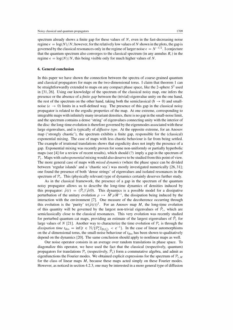
Noisy classical and quantum propagators 1709
spectrum already shows a finite gap for these values of N , even in the fast-decreasing noiseregime ε = log(N)/N ; however, for the relatively low values of N shown in the plots, the gap isgoverned by the classical resonances only in the regime of larger noise ε = N−1/2. I conjecturethat the quantum spectrum also converges to the classical spectrum (in any annulus Rr ) in theregime ε = log(N)/N , this being visible only for much higher values of N .
6. General conclusion
In this paper we have shown the connection between the spectra of coarse-grained quantumand classical propagators for maps on the two-dimensional torus. I claim that theorem 1 canbe straightforwardly extended to maps on any compact phase space, like the 2-sphere S2 usedin [31, 26]. Using our knowledge of the spectrum of the classical noisy map, one infers thepresence or the absence of a finite gap between the (trivial) eigenvalue unity on the one hand,the rest of the spectrum on the other hand, taking both the semiclassical (h → 0) and small-noise (ε → 0) limits in a well-defined way. The presence of this gap in the classical noisypropagator is related to the ergodic properties of the map. At one extreme, corresponding tointegrable maps with infinitely many invariant densities, there is no gap in the small-noise limit,and the spectrum contains a dense ‘string’ of eigenvalues connecting unity with the interior ofthe disc: the long-time evolution is therefore governed by the eigenmodes associated with theselarge eigenvalues, and is typically of diffusive type. At the opposite extreme, for an Anosovmap (‘strongly chaotic’), the spectrum exhibits a finite gap, responsible for the (classical)exponential mixing. The case of maps with less chaotic behaviour is far from being settled.The example of irrational translations shows that ergodicity does not imply the presence of agap. Exponential mixing was recently proven for some non-uniformly or partially hyperbolicmaps (see [4] for a review of recent results), which should (?) imply a gap in the spectrum ofPε . Maps with subexponential mixing would also deserve to be studied from this point of view.The more general case of maps with mixed dynamics (where the phase space can be dividedbetween ‘regular islands’ and a ‘chaotic sea’) was mostly investigated numerically [26, 31];one found the presence of both ‘dense strings’ of eigenvalues and isolated resonances in thespectrum of Pε . This (physically relevant) type of dynamics certainly deserves further study.
As in the classical framework, the presence of a gap in the spectrum of the quantumnoisy propagator allows us to describe the long-time dynamics of densities induced bythis propagator: ρ(t) = (Pε)
t ρ(0). This dynamics is a possible model for a dissipativeperturbation of the unitary evolution ρ �→ MtρM−t , the dissipation being induced by theinteraction with the environment [7]. One measure of the decoherence occurring throughthis evolution is the ‘purity’ tr(ρ(t))2. For an Anosov map M , the long-time evolutionof this quantity will be governed by the largest non-trivial eigenvalues of Pε , which aresemiclassically close to the classical resonances. This very evolution was recently studiedfor perturbed quantum cat maps, providing an estimate of the largest eigenvalues of Pε forlarge values of N [21]. Another way to characterize the time evolution of Pε is through thedissipation time tdiss = inf{t ∈ N/‖P t
ε‖B(L20)
< e−1}. In the case of linear automorphismson the d-dimensional torus, the small-noise behaviour of tdiss has been shown to qualitativelydepend on the dynamics [20]. The same conclusion should apply to nonlinear maps as well.
Our noise operator consists in an average over random translations in phase space. Todiagonalize this operator, we have used the fact that the classical (respectively, quantum)propagators for translations Pv (respectively, Pv) form a commutative algebra, and admit aseigenfunctions the Fourier modes. We obtained explicit expressions for the spectrum of Pε,M
for the class of linear maps M , because these maps acted simply on these Fourier modes.However, as noticed in section 4.2.3, one may be interested in a more general type of diffusion

1710 S Nonnenmacher
operator, like the one defined in equation (21). The spectrum of D{Hj }ε ◦PM for a given map M
should be qualitatively independent of the family of Hamiltonians {Hj }, as long as the operator
D{Hj }ε has the same characteristics as the coarse-graining Dε , namely it leaves almost invariant
some ‘soft modes’, while killing fast-oscillating modes. In particular, for M an Anosov map,the outer spectrum of D
{Hj }ε ◦ PM should converge to the set of resonances {λi}, and the rest
is contained in a smaller disc, in the limit ε → 0. For an integrable map, the eigenvalues willnot pointwise converge to those of DεPM , but they should also accumulate along a ‘string’touching unity.
Our choice for the super-operator Dε was inspired by its classical analogue, as well as itsrelevance to modellize the ‘quantum noise’. However, in some quantum systems experiencing(weak) interaction with the environment, the effective ‘noise’ or ‘decoherence’ superoperatormay have no obvious classical analogue; this seems to be the case for instance in nuclearmagnetic resonance experiments aiming at realizing a ‘quantum computer’ [15]. The quantumHilbert space is composed of a sequence of n spins, so it is isomorphic with the torusHilbert space HN for N = 2n (each spin corresponds to a binary digit of the position qj ).The decoherence operator acting on such a system (for a small number of spins) has beenexperimentally measured, it resembles the product of operators acting independently on theindividual spins, and therefore does not enter in the family of diffusion operators describedin this paper; in particular, such a decoherence operator seems to have no obvious classicalcounterpart. Conjugating this type of decoherence operator with a unitary evolution (typically,the finite Fourier transform J ) may lead to a drastically different spectrum from the one shownin figure 1 (right), not excluding the presence of a gap.
Acknowledgments
I thank M Zirnbauer and the Institut fur theoretische Physik, Universitat zu Koln, where thiswork was initiated. I am grateful to V Baladi and S De Bievre for respectively pointingout [8, 20] to me, and thank S Keppeler for his insight on integrable maps. I had interestingdiscussions on the whole subject with M Saraceno and I Garcia Mata.
Appendix A
Appendix A.1. Classical nonlinear shear: spectrum of truncated Toeplitz matrices
This appendix describes the spectrum of the noisy classical propagator for a nonlinear shear(section 3.2.3). In each invariant subspace Vn = {e2iπnq ρ(p)} (n ∈ Z
∗), the Perron–Frobeniusoperator P acts as a multiplication of the function ρ(p) on the circle T
1 � t = e2iπp by
an(e2iπp)
def= e−2iπn(sp+F ′(p)) =∑m∈Z
an(m)e2iπmp. (27)
Note that an(t) = (a1(t))n. In the Fourier basis, this multiplication has the form of an infinite
Laurent matrix L(an), with entries L(an)ij = an(i − j). From standard results, the spectrumof P|Vn
is absolutely continuous, with support in the range of the function an(t) (here, the unitcircle).
We consider the coarse-graining consisting in a sharp truncation in Fourier space:K(ξ) = �(ξ1)�(ξ2). The noisy propagator Pε then acts on Vn as the matrix L(an) truncatedto the block {|m|, |m′| � ε−1}, or equivalently as {1 � m, m′ � 2ε−1 + 1}. We assume thatthe smooth function an(t) on T
1 can be continued to an analytic (or meromorphic) functionon C
∗ (for the linear shear, one has an(z) = z−sn). Then, for any r > 0 and any ε > 0,

Noisy classical and quantum propagators 1711
the spectrum of this truncated matrix is contained in the convex hull of the curve an(rT1)
[11, proposition 2.17 and section 5.8]. For the linear shear, these curves are the circles centredat the origin, so the spectrum reduces to {0}, as expected. If the perturbation F ′ is small,these curves are deformations of circles, some of which remain in a small neighbourhood ofthe origin. As a concrete example, the perturbation F(p) = (α/2π) cos(2πp) leads to thefunction a−1(z) = zs exp{πα(1/z− z)}. The curves a−1(rT
1) satisfy
∀r > 0, |z| = r ⇒ |a−1(z)| � rs exp
(πα
∣∣∣∣1
r− r
∣∣∣∣)
.
We assume that s > 0. For a small perturbation (α � 1), the function on the right-hand sidehas a minimum of value amin(α) � (παe/s)s. This implies that for any n, the spectrum ofPε|Vn
is contained in the disc of radius (amin(α))|n| for any ε > 0 (we have used the symmetrya−n = an).
For a more general perturbation 2πF ′(t) = ∑m�1 fmtm + c.c. one can use the bound
2π |!F ′(rt)| � sup(g(r), g(1/r)) with g(r)def= ∑
m�1 |fm|rm. If g(r) is ‘small’, then thefunction rs exp(g(1/r)) has a minimum amin � 1 on R
∗+. This implies that the spectrum of
Pε|Vnis contained, for any ε, in the disc around the origin of radius a
|n|min.
Appendix A.2. Quantum nonlinear shear
The results of the previous appendix can be easily adapted to the quantized nonlinear shear.The latter is defined as the composition of the quantum linear shear S with the Floquet operatorcorresponding to the Hamiltonian F (see section 3.2.3): the quantum map reads Se−2iπNF . Itsaction is diagonal in the impulsion basis {|pj 〉N } of HN (pj = j/N , with j ∈ ZN ):
Se−iF /h|pj 〉N = e−2iπN((s/2)p2j +F(pj ))|pj 〉N.
Since s is even, this expression is well defined for any j ∈ ZN . As we now show, itallows us to express the action of the propagator P on the quantum translations Tk/N . Takingk = (m, n) ∈ Z
2N , this translation can be decomposed as
Tk/N =∑j∈ZN
|pj+n〉〈pj |e−2iπm(pj +n/2N).
P acts inside each subspace Vn,N = Span {T(m,n)/N , m ∈ ZN } = Span {|pj+n〉〈pj |, j ∈ ZN }.The propagator P indeed multiplies each |pj+n〉〈pj | by the phase An,N(e2iπ(pj +n/2N)), with thefunction An,N on T
1 defined as:
An,N(e2iπp)def= e−2iπsnpe−2iπN [F(p+n/2N)−F(p−n/2N)] =
∑m∈Z
An,N (m)e2iπmp.
An,N(t) uniformly converges to the function an(t) of equation (27) in the limit N →∞. Forour example F(p) = (α/2π) cos(2πp), it takes the concise form
An,N(e2iπp) = e−2iπn(sp−αn,N sin(2πp))
with
αn,N = αN
πnsin
(πn
N
)= α
(1 + O
(( n
N
)2))
.
From there, we can express the action of P on the quantum translations:
PT(m,n)/N =∑l∈Z
T(m−l,n)/N An,N (l) =∑l∈ZN
T(l,n)/N A′n,N (m− l)

1712 S Nonnenmacher
where A′n,N (m) =∑ν∈Z
(−1)nνAn,N (m + νN). Therefore, P acts on Vn,N through the N ×N
Toeplitz matrix with coefficients A′n,N (m). If we truncate this matrix to the size {|l|, |l′| � ε−1}with ε−1 � N , we only take into account the coefficients with |m| � 2ε−1. Since An,N isa smooth function, each of these coefficients is the sum of a ‘dominant’ term An,N (m) anda ‘remainder’. For our example, the classical coefficients are given by Bessel functions:an(m) = Jm+sn(2πnα), and the same for An,N (m), replacing α by αn,N . These coefficientstherefore satisfy |An,N (m)| � C((nα)|m+ns|/|m + ns|!), so that the remainder is uniformlybounded above by (C ′α/εN)N/2 for large N . If we call P�
ε|Vn,Nthe truncated Toeplitz matrix
with coefficients An,N (m), we get the estimate:
‖Pε|Vn,N− P�
ε|Vn,N‖ � (2ε−1 + 1)
(C ′αεN
)N/2
.
This estimate implies that the spectra of both matrices cannot be at a distance larger thanO((εN)−εN/4). The matrix P�
ε|Vn,Nmay be analysed along the same lines as Pε|Vn
in theprevious appendix. Its spectrum is contained for any ε > 0 and any r > 0 in the convex hullof An,N(rT
1), which converges to the convex hull of an(rT1) when N →∞.
References
[1] Agam O and Blum G 2000 The leading Ruelle resonances of chaotic maps Phys. Rev. E 62 1977–82[2] Andreev A V, Agam O, Altshuler B L and Simons B D 1996 Semiclassical field theory approach to quantum
chaos Nucl. Phys. B 482 536–66[3] Arnold V I and Avez A 1968 Ergodic Problems of Classical Mechanics (New York: Benjamin)[4] Baladi V 2001 Spectrum and statistical properties of chaotic dynamics Prog. Math. 201 203–23[5] Baladi V and Baillif M 2002 Kneading determinants and spectra of transfer operators in higher dimensions, the
isotropic case Preprint math.DS/0211343/[6] Baladi V and Young L-S 1993 On the spectra of randomly perturbed expanding maps Commun. Math. Phys.
156 355–85Baladi V and Young L-S 1994 Commun. Math. Phys. 166 219–20 (erratum)
[7] Bianucci P, Paz J P and Saraceno M 2002 Decoherence for classically chaotic quantum maps Phys. Rev. E 65046226
[8] Blank M, Keller G and Liverani C 2002 Ruelle–Perron–Frobenius spectrum for Anosov maps Nonlinearity 151905–73
[9] Bogomolny E B 1992 Semiclassical quantization of multidimensional systems Nonlinearity 5 805–66[10] Bonifacio R, Schwendimann P and Haake F 1971 Quantum statistical theory of superradiance Phys. Rev. A 4
302–13 and 854–64[11] Bottcher A and Silbermann B 1999 Introduction to Large Truncated Toeplitz Matrices (Berlin: Springer)[12] Bouzouina A and De Bièvre S 1996 Equipartition of the eigenfunctions of quantized ergodic maps on the torus
Commun. Math. Phys. 178 83–105[13] Braun D 1999 Spectral properties of dissipative chaotic quantum maps Chaos 9 730–7
Braun D 2001 Dissipative Quantum Chaos and Decoherence (Springer Tracts in Modern Physics vol 172)(Heidelberg: Springer)
[14] Caldeira A O and Leggett A J 1985 Influence of damping on quantum interference: an exactly soluble modelPhys. Rev. A 31 1059–66
[15] Childs A M, Chuang I L and Leung D W 2001 Realization of quantum process tomography in NMR Phys. Rev.A 64 012314
Vandersypen L M K et al 2001 Experimental realization of Shor’s quantum factoring algorithm using nuclearmagnetic resonance Nature 414 883–7
[16] Conley C and Zehnder E 1983 The Birkhoff–Lewis fixed point theorem and a conjecture of V I Arnold Invent.Math. 73 33–49
[17] Chuang I L and Nielsen M A 2000 Quantum Computation and Quantum Information (Cambridge: CambridgeUniversity Press)
[18] Cornfeld I P, Fomin S V and Sinai Ya G 1982 Ergodic Theory (Berlin: Springer)

Noisy classical and quantum propagators 1713
[19] Degli Esposti M, Graffi S and Isola S 1995 Classical limit of the quantized hyperbolic toral automorphismsCommun. Math. Phys. 167 471–507
[20] Fannjiang A and Wołowski L 2003 Noise induced dissipation in Lebesgue-measure preserving maps ond-dimensional torus Preprint
[21] Garcia Mata I, Saraceno M and Spina M E 2003 Classical decays in decoherent quantum maps Preprintnlin.CD/0301025
[22] Habib S, Shizume K and Zurek W H 1998 Decoherence, chaos and the correspondence principle Phys. Rev.Lett. 80 4361
[23] Hannay J H and Berry M V 1980 Quantization of linear maps on a torus-Fresnel diffraction by a periodic gratingPhysica D 1 267–90
Degli Esposti M 1993 Quantization of the orientation preserving automorphisms of the torus Ann. Inst. HPoincaré 58 323–41
[24] Katok A and Hasselblatt B 1995 Introduction to the Modern Theory of Dynamical Systems (Cambridge:Cambridge University Press)
[25] Keating J, Mezzadri F and Robbins J 1999 Quantum boundary conditions for torus maps Nonlinearity 12 579–91[26] Khodas M, Fishman S and Agam O 2000 Relaxation to the invariant density for kicked rotor Phys. Rev. 62
4769–83Fishman S and Rahav S 2002 Relaxation and noise in chaotic systems Lecture Notes (Ladek Winter School)
nlin.CD/0204068[27] Kifer Yu 1988 Random Perturbations of Dynamical Systems (Basel: Birkhauser)[28] Kurlberg P and Rudnick Z 2001 On quantum ergodicity for linear maps of the torus Commun. Math. Phys. 222
201–27[29] Kurlberg P 2002 On the order of unimodular matrices modulo integers Preprint math.NT/0202053[30] Lindblad G 1976 On the generators of quantum dynamical semigroups Commun. Math. Phys. 48 119–30[31] Manderfeld C, Weber J and Haake F 2001 Classical versus quantum time evolution of (quasi-) probability
densities at limited phase-space resolution J. Phys. A: Math. Gen. 34 9893–905Weber J, Haake F, Braun P A, Manderfeld C and Seba P 2001 Resonances of the Frobenius–Perron operator for
a Hamiltonian map with a mixed phase space J. Phys. A: Math. Gen. 34 7195–211[32] Marklof J and Rudnick Z 2000 Quantum unique ergodicity for parabolic maps Geom. Funct. Anal. 10 1554–78[33] Nonnenmacher S and Zirnbauer M R 2002 Det–det correlations for quantum maps: dual pair and saddle-point
analyses J. Math. Phys. 43 2214–40[34] Ostruszka A and Zyckzkowski K 2001 Spectrum of the Frobenius–Perron operator for systems with stochastic
perturbation Phys. Lett. A 289 306–12[35] Palla G, Vattay G, Voros A, Søndergaard N and Dettmann C-P 2001 Noise corrections to stochastic trace formulas
Found. Phys. 31 641–57[36] Parry W and Pollicott M 1990 Zeta functions and the periodic orbit structure of hyperbolic dynamics Astérisque
vol 187–8, Société mathématique de France, Paris[37] Percival I and Vivaldi F 1987 Arithmetical properties of strongly chaotic motions Physica D 25 105–30[38] Prosen T 2002 Chaotic resonances in quantum many-body dynamics Preprint[39] Reed M and Simon B 1972 Methods of Modern Mathematical Physics, I: Functional Analysis (New York:
Academic)[40] Ruelle D 1986 Locating resonances for axiom A dynamical systems J. Stat. Phys. 44 281–92
Ruelle D 1987 One-dimensional Gibbs states and axiom-A diffeomorphisms J. Diff. Geom. 25 117–37[41] Rugh H H 1992 The correlation spectrum for hyperbolic analytic maps Nonlinearity 5 1237–63
Rugh H H 1996 Generalized Fredholm determinants and Selberg zeta functions for axiom A dynamical systemsErgod. Theory Dyn. Syst. 16 805–19
[42] Tabor M 1983 A semiclassical quantization of area-preserving maps Physica D 6 195–210[43] Takahashi K 1989 Distribution in classical and quantum mechanics Prog. Theor. Phys. Suppl. 98 109–56[44] Zelditch S 1997 Index and dynamics of quantized contact transformations Ann. Inst. Fourier 47 305–65