spectral methods for multi-scale feature extraction … spectral methods for multi-scale feature...
TRANSCRIPT

Spectral Methods for
Multi-Scale Feature Extraction and Data Clustering
by
Srinivas Chakra Chennubhotla
A thesis submitted in conformity with the requirementsfor the degree of Doctor of Philosophy
Graduate Department of Computer ScienceUniversity of Toronto
Copyright c© 2004 by Srinivas Chakra Chennubhotla

Abstract
Spectral Methods for
Multi-Scale Feature Extraction and Data Clustering
Srinivas Chakra Chennubhotla
Doctor of Philosophy
Graduate Department of Computer Science
University of Toronto
2004
We address two issues that are fundamental to the analysis of naturally-occurring datasets:
how to extract features that arise at multiple-scales and how to cluster items in a dataset
using pairwise similarities between the elements. To this end we present two spectral
methods: (1) Sparse Principal Component Analysis S-PCA — a framework for learning
a linear, orthonormal basis representation for structure intrinsic to a given dataset; and
(2) EigenCuts — an algorithm for clustering items in a dataset using their pairwise-
similarities.
S-PCA is based on the discovery that natural images exhibit structure in a low-
dimensional subspace in a local, scale-dependent form. It is motivated by the observation
that PCA does not typically recover such representations, due to its single minded pursuit
of variance. In fact, it is widely believed that the analysis of second-order statistics alone
is insufficient for extracting multi-scale structure from data and there are many proposals
in the literature showing how to harness higher-order image statistics to build multi-
scale representations. In this thesis, we show that resolving second-order statistics with
suitably constrained basis directions is indeed sufficient to extract multi-scale structure.
In particular, S-PCA basis optimizes an objective function which trades off correlations
among output coefficients for sparsity in the description of basis vector elements. Using
S-PCA we present new approaches to the problem of constrast-invariant appearance
ii

detection, specifically eye and face detection.
EigenCuts is a clustering algorithm for finding stable clusters in a dataset. Using
a Markov chain perspective, we derive an eigenflow to describe the flow of probability
mass due to the Markov chain and characterize it by its eigenvalue, or equivalently, by
the halflife of its decay as the Markov chain is iterated. The key insight in this work
is that bottlenecks between weakly coupled clusters can be identified by computing the
sensitivity of the eigenflow’s halflife to variations in the edge weights. The EigenCuts
algorithm performs clustering by removing these identified bottlenecks in an iterative
fashion. As an efficient step in this process we also propose a specialized hierarchical
eigensolver suitable for large stochastic matrices.
iii

Contents
1 Introduction 1
1.1 Image Understanding . . . . . . . . . . . . . . . . . . . . . . . . . . . . . 1
1.2 Contributions . . . . . . . . . . . . . . . . . . . . . . . . . . . . . . . . . 3
1.3 Overview . . . . . . . . . . . . . . . . . . . . . . . . . . . . . . . . . . . . 4
2 Identifying Object-Specific Multi-Scale Structure 6
2.1 Motivation . . . . . . . . . . . . . . . . . . . . . . . . . . . . . . . . . . . 6
2.2 Decorrelation, Sparsity and Independence . . . . . . . . . . . . . . . . . . 10
2.2.1 Datasets . . . . . . . . . . . . . . . . . . . . . . . . . . . . . . . . 10
2.2.2 Linear Synthesis Model . . . . . . . . . . . . . . . . . . . . . . . . 11
2.2.3 Principal Component Analysis (PCA) . . . . . . . . . . . . . . . . 12
Results from PCA . . . . . . . . . . . . . . . . . . . . . . . . . . 14
2.2.4 Sparse Coding and ICA . . . . . . . . . . . . . . . . . . . . . . . 17
Results from Sparse Coding . . . . . . . . . . . . . . . . . . . . . 23
2.3 Object-Specific Multi-Scale Structure . . . . . . . . . . . . . . . . . . . . 26
3 Sparse Principal Component Analysis: S-PCA 31
3.1 Introduction . . . . . . . . . . . . . . . . . . . . . . . . . . . . . . . . . . 31
3.2 Encouraging Sparsity . . . . . . . . . . . . . . . . . . . . . . . . . . . . . 32
3.3 S-PCA Pairwise Rotation Algorithm . . . . . . . . . . . . . . . . . . . . 33
3.3.1 Details . . . . . . . . . . . . . . . . . . . . . . . . . . . . . . . . . 35
iv

3.4 S-PCA on Datasets With Known Structure . . . . . . . . . . . . . . . . . 39
3.4.1 Low-Pass Filtered Noise Ensemble . . . . . . . . . . . . . . . . . . 39
3.4.2 Band-Pass Filtered Noise Ensemble . . . . . . . . . . . . . . . . . 46
3.4.3 Noisy Sine Waves . . . . . . . . . . . . . . . . . . . . . . . . . . . 46
3.4.4 Garbage In, “Garbage” Out? . . . . . . . . . . . . . . . . . . . . 50
3.5 S-PCA on Natural Ensembles . . . . . . . . . . . . . . . . . . . . . . . . 50
3.5.1 Facelets . . . . . . . . . . . . . . . . . . . . . . . . . . . . . . . 54
3.5.2 Handlets . . . . . . . . . . . . . . . . . . . . . . . . . . . . . . 54
3.5.3 Wavelets . . . . . . . . . . . . . . . . . . . . . . . . . . . . . . 56
3.5.4 Flowlets . . . . . . . . . . . . . . . . . . . . . . . . . . . . . . 58
3.6 Enforcing Sparsity by Coring . . . . . . . . . . . . . . . . . . . . . . . . 60
3.6.1 Iterative Image Reconstruction . . . . . . . . . . . . . . . . . . . 61
3.6.2 Eyelets . . . . . . . . . . . . . . . . . . . . . . . . . . . . . . . 63
3.7 Related Work . . . . . . . . . . . . . . . . . . . . . . . . . . . . . . . . . 68
4 Contrast-Invariant Appearance-Based Detection 71
4.1 Introduction . . . . . . . . . . . . . . . . . . . . . . . . . . . . . . . . . . 71
4.2 Datasets . . . . . . . . . . . . . . . . . . . . . . . . . . . . . . . . . . . . 73
4.3 Detection Model – I . . . . . . . . . . . . . . . . . . . . . . . . . . . . . . 74
4.3.1 Contrast Model for an Object-Specific Ensemble . . . . . . . . . . 75
4.3.2 Principal Subspace and its Complement . . . . . . . . . . . . . . 77
4.3.3 Detection Strategy . . . . . . . . . . . . . . . . . . . . . . . . . . 81
4.3.4 Results . . . . . . . . . . . . . . . . . . . . . . . . . . . . . . . . . 82
4.4 Detection Model – II . . . . . . . . . . . . . . . . . . . . . . . . . . . . . 86
4.4.1 Weber-Contrast Normalization . . . . . . . . . . . . . . . . . . . . 87
4.4.2 S-PCA Representation: W,B . . . . . . . . . . . . . . . . . . . . 90
4.4.3 Perceptual Distance Normalization . . . . . . . . . . . . . . . . . 90
4.4.4 Detection Strategy . . . . . . . . . . . . . . . . . . . . . . . . . . 94
v

4.4.5 Results . . . . . . . . . . . . . . . . . . . . . . . . . . . . . . . . . 95
Eyes/Non-Eyes: . . . . . . . . . . . . . . . . . . . . . . . . . . . . 95
Faces/Non-Faces: . . . . . . . . . . . . . . . . . . . . . . . . . . . 96
Comparison with Support Vector Machine (SVM) . . . . . . . . . 98
4.5 Conclusion . . . . . . . . . . . . . . . . . . . . . . . . . . . . . . . . . . . 103
5 S-PCA: Conclusions and Future Work 104
5.1 Future Work . . . . . . . . . . . . . . . . . . . . . . . . . . . . . . . . . . 105
5.1.1 Sparse-Infomax . . . . . . . . . . . . . . . . . . . . . . . . . . 105
5.1.2 Encouraging Sparsity with a Mixture-of-Gaussian Prior . . . . . . 107
6 Spectral Clustering 110
6.1 Visual Grouping . . . . . . . . . . . . . . . . . . . . . . . . . . . . . . . . 110
6.2 Graph-Theoretic Partitioning . . . . . . . . . . . . . . . . . . . . . . . . 111
6.2.1 Graph Formulation . . . . . . . . . . . . . . . . . . . . . . . . . . 111
6.2.2 Cut Measures / Criterion . . . . . . . . . . . . . . . . . . . . . . . 113
6.3 Spectral-based Methods . . . . . . . . . . . . . . . . . . . . . . . . . . . 115
6.3.1 NCut algorithm . . . . . . . . . . . . . . . . . . . . . . . . . . . . 116
6.3.2 K–Means Spectral Clustering . . . . . . . . . . . . . . . . . . . . 116
6.3.3 Random Walks and Normalized Cuts . . . . . . . . . . . . . . . . 117
6.3.4 Assumption of piecewise constancy . . . . . . . . . . . . . . . . . 119
7 EigenCuts: A Spectral Clustering Algorithm 122
7.1 Introduction . . . . . . . . . . . . . . . . . . . . . . . . . . . . . . . . . . 122
7.2 From Affinities to Markov Chains . . . . . . . . . . . . . . . . . . . . . . 123
7.2.1 Notation and basic parameters . . . . . . . . . . . . . . . . . . . . 123
7.2.2 Markov Chain . . . . . . . . . . . . . . . . . . . . . . . . . . . . . 124
7.2.3 Markov Chain Propagation . . . . . . . . . . . . . . . . . . . . . 126
7.2.4 Perturbations to the Stationary Distribution . . . . . . . . . . . . 127
vi
7.3 EigenFlows and Perturbation Analysis . . . . . . . . . . . . . . . . . . . 130
7.3.1 EigenFlows . . . . . . . . . . . . . . . . . . . . . . . . . . . . . . 130
7.3.2 Perturbation Analysis . . . . . . . . . . . . . . . . . . . . . . . . 133
7.3.3 What do half-life sensitivities reveal? . . . . . . . . . . . . . . . . 136
7.4 EigenCuts: A Basic Clustering Algorithm . . . . . . . . . . . . . . . . 138
7.4.1 Iterative Cutting Process . . . . . . . . . . . . . . . . . . . . . . . 140
7.5 Experiments . . . . . . . . . . . . . . . . . . . . . . . . . . . . . . . . . . 146
7.6 Discussion . . . . . . . . . . . . . . . . . . . . . . . . . . . . . . . . . . . 148
8 Hierarchical Representation of Transition Matrices 152
8.1 Previous Work . . . . . . . . . . . . . . . . . . . . . . . . . . . . . . . . 153
8.2 Markov Chain Terminology . . . . . . . . . . . . . . . . . . . . . . . . . 154
8.3 Building a Hierarchy of Transition Matrices . . . . . . . . . . . . . . . . 155
8.3.1 Deriving Coarse-Scale Stationary Distribution . . . . . . . . . . . 156
8.3.2 Deriving the Coarse-Scale Transition Matrix . . . . . . . . . . . . 159
8.3.3 Selecting Kernels . . . . . . . . . . . . . . . . . . . . . . . . . . . 160
8.4 Fast EigenSolver . . . . . . . . . . . . . . . . . . . . . . . . . . . . . . . 163
8.4.1 Interpolation Results . . . . . . . . . . . . . . . . . . . . . . . . . 165
9 Multi-Scale EigenCuts 174
9.1 Introduction . . . . . . . . . . . . . . . . . . . . . . . . . . . . . . . . . . 174
9.2 Algorithm Details . . . . . . . . . . . . . . . . . . . . . . . . . . . . . . . 174
9.3 Results . . . . . . . . . . . . . . . . . . . . . . . . . . . . . . . . . . . . . 182
10 EigenCuts: Conclusions 183
Bibliography 185
vii

Chapter 1
Introduction
1.1 Image Understanding
One of the goals in the study of computer vision is to devise algorithms that help us
understand and recover useful properties of the scene from one or more images. This
inverse problem is difficult because information is lost about the three-dimensional world
when it is projected on to a two-dimensional image. However, our visual systems seem
very adept at performing this task. For example, the objects (or well-defined parts of
objects) in the scene are perceived as coherent visual groups in the image and the quality
of the percept tends to be consistent across observers. Typically, subjects agree on
the properties that they ascribe to objects in the scene, say in terms of colour, texture
or shape attributes. Furthermore, if the objects are familiar, then they tend to get
recognized as such. Thus, two processes: perceptual grouping/organization and object
recognition, form the core of image understanding.
The importance of perceptual grouping and organization in visual perception has been
laid out many years ago by the Gestaltist school [120]. For this thesis we motivate the
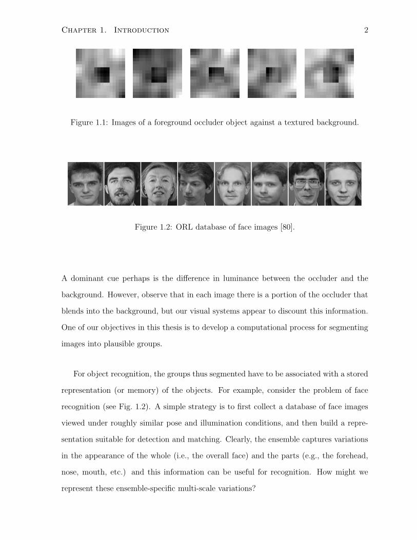
grouping problem by inviting the reader to segment images shown in Fig. 1.1. Observers
report perceiving two “things” – a foreground object occluding a textured background.
1
Chapter 1. Introduction 2
Figure 1.1: Images of a foreground occluder object against a textured background.
Figure 1.2: ORL database of face images [80].
A dominant cue perhaps is the difference in luminance between the occluder and the
background. However, observe that in each image there is a portion of the occluder that
blends into the background, but our visual systems appear to discount this information.
One of our objectives in this thesis is to develop a computational process for segmenting
images into plausible groups.
For object recognition, the groups thus segmented have to be associated with a stored
representation (or memory) of the objects. For example, consider the problem of face
recognition (see Fig. 1.2). A simple strategy is to first collect a database of face images
viewed under roughly similar pose and illumination conditions, and then build a repre-
sentation suitable for detection and matching. Clearly, the ensemble captures variations
in the appearance of the whole (i.e., the overall face) and the parts (e.g., the forehead,
nose, mouth, etc.) and this information can be useful for recognition. How might we
represent these ensemble-specific multi-scale variations?
Chapter 1. Introduction 3
1.2 Contributions
In this thesis, we address two issues that we believe are fundamental to the analysis of
high-dimensional, object-specific ensembles of visual, and other perceptual, data:
• how to extract features that arise at multiple-scales;
• how to cluster, or group, items in a dataset using pairwise similarities between the
elements.
To this end, we present the following two spectral methods:
1. Sparse Principal Component Analysis (S-PCA) — a framework for learning
a linear, orthonormal basis representation for structure intrinsic to a given dataset;
2. EigenCuts — an algorithm for clustering items in a dataset using their pairwise-
similarities.
S-PCA is based on the discovery that natural images exhibit structure in a low-
dimensional subspace in a local, scale-dependent form. It is motivated by the observation
that PCA does not typically recover such representations. In fact, it is widely believed
that the analysis of second-order statistics alone is insufficient for extracting multi-scale
structure from data and there are many proposals in the literature showing how to harness
higher-order image statistics to build multi-scale representations. In this thesis, we show
that resolving second-order statistics with suitably constrained basis directions is indeed
sufficient to extract multi-scale structure. The formulation of S-PCA is novel in that it
successfully computes multi-scale representations for a variety of natural image ensembles
including face images, images from outdoor scenes and a database of optical flow vectors
representing a motion class.
Using S-PCA, we present new approaches to the problem of contrast-invariant ap-
pearance detection. The goal is to classify object-specific images (eg. face images) from

Chapter 1. Introduction 4
generic background patches. The novel contribution of this work is the design of a percep-
tual distortion measure for image similarity, i.e., comparing the appearance of an object
to its reconstruction from the principal subspace. We demonstrate our approach on two
different datasets: separating eyes from non-eyes and classifying faces from non-faces.
EigenCuts is a clustering algorithm for finding stable clusters in a dataset. Using
a Markov chain perspective, we characterize the spectral properties of the matrix of
transition probabilities, from which we derive eigenflows along with their halflives. An
eigenflow describes the flow of probability mass due to the Markov chain, and it is
characterized by its eigenvalue, or equivalently, by the halflife of its decay as the Markov
chain is iterated. A ideal stable cluster is one with zero eigenflow and infinite half-life.
The key insight in this work is that bottlenecks between weakly coupled clusters can be
identified by computing the sensitivity of the eigenflow’s halflife to variations in the edge
weights. The EigenCuts algorithm performs clustering by removing these identified
bottlenecks in an iterative fashion.
Also, in this thesis we propose a specialized eigensolver suitable for large stochas-
tic matrices with known stationary distributions. In particular, we exploit the spectral
properties of the Markov transition matrix to generate hierarchical, successively lower-
dimensional approximations to the full transition matrix. The eigen problem is solved
directly at the coarsest level of representation. The approximate eigen solution is then in-
terpolated over successive levels of the hierarchy, using a small number of power iterations
to correct the solution at each stage. To show the effectiveness of this approximation, we
present a multi-scale version of the EigenCuts algorithm.
1.3 Overview
This thesis is organized in two parts. In the first part we discuss S-PCA and in the
second we study spectral clustering.

Chapter 1. Introduction 5
We begin our discussion in Chapter 2 with the following question: how to identify
object-specific multi-scale structure? We review the observation that natural images ex-
hibit structure in a low-dimensional subspace in a sparse, scale-dependent form. Based
on this discovery, we propose a new learning algorithm called S-PCA in Chapter 3.
In particular, S-PCA basis optimizes an objective function which trades off correlations
among output coefficients for sparsity in the description of basis vector elements. This
objective function is minimized by a simple, robust and highly scalable algorithm con-
sisting of successive planar rotations of pairs of basis vectors. We discuss the algorithm
in detail and demonstrate results on a wide variety of ensembles.
In Chapter 4 we demonstrate an application of this model for appearance-based object
detection using two different datasets: separating eyes from non-eyes and classifying faces
from non-faces. We end the first part of this thesis in Chapter 5, with a discussion on
two possible new directions that we can undertake with S-PCA.
We begin the second part of this thesis in Chapter 6 with an introduction to spectral
clustering. In Chapter 7 we present a new clustering algorithm called EigenCuts based
on a Markov chain perspective of spectral clustering. The significant time complexity
of solving eigenvalue problems in spectral clustering motivated us to build a specialized
eigensolver suitable for large stochastic matrices with known stationary distributions
(Chapter 8). In particular, we exploit the spectral properties of the Markov transi-
tion matrix to generate hierarchical, successively lower-ranked approximations to the full
transition matrix. To show the effectiveness of this approximation, we also present a
multi-scale version of the EigenCuts algorithm. We conclude the second part of this
thesis in Chapter 10.
Chapter 2
Identifying Object-Specific
Multi-Scale Structure
2.1 Motivation
Our goal is to identify and represent structure inherent to high-dimensional object-specific
ensembles of visual, and other perceptual, data. In this thesis we consider several dif-
ferent natural image ensembles: images sampled from outdoor environments (Fig. 2.1);
face images acquired from roughly similar viewpoints (Fig. 1.2); images of a gesturing
hand (Fig. 2.4); and vector-valued optical flow measurements collected from motion se-
quences. It is well known that natural image ensembles exhibit multi-scale structure.
Typically, fine-scale structure is spatially localized while coarse-scale structure is spa-
tially distributed. As an example, consider the database of face images acquired under
roughly similar viewpoints and illumination conditions (Fig. 1.2). Here, we expect to see
variations in the appearance of the whole (overall face), the parts (forehead, nose, mouth,
etc.), and then perhaps some fine details (moles etc.). We are interested in representing
these ensemble-specific multi-scale variations.
There are at least two approaches to take for building a multi-scale representation: (1)
6
Chapter 2. Identifying Object-Specific Multi-Scale Structure 7
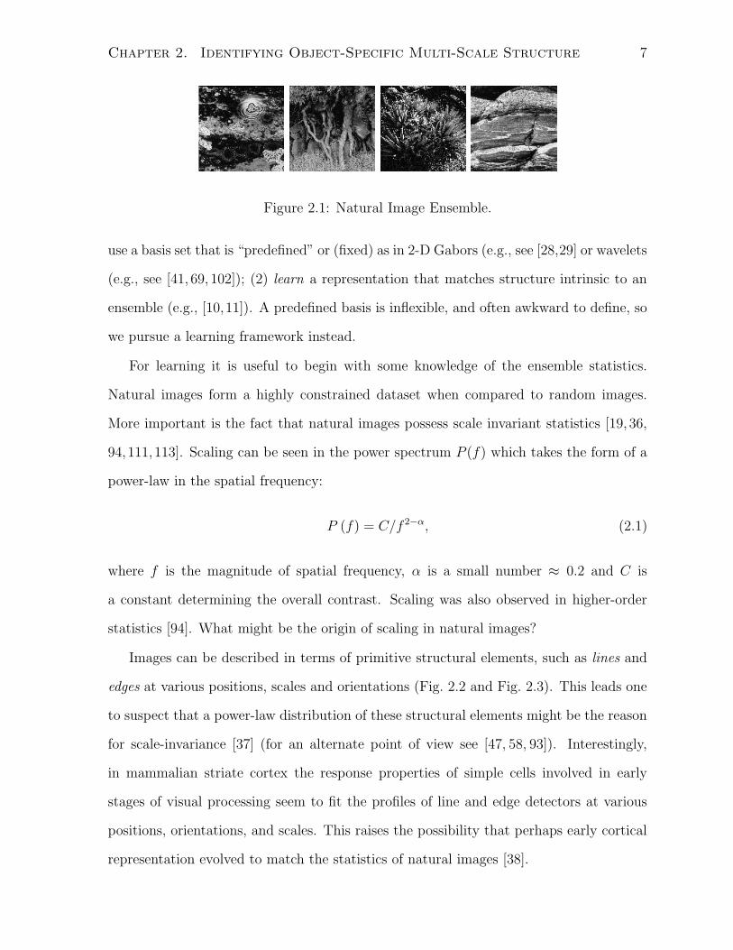
Figure 2.1: Natural Image Ensemble.
use a basis set that is “predefined” or (fixed) as in 2-D Gabors (e.g., see [28,29] or wavelets
(e.g., see [41, 69, 102]); (2) learn a representation that matches structure intrinsic to an
ensemble (e.g., [10,11]). A predefined basis is inflexible, and often awkward to define, so
we pursue a learning framework instead.
For learning it is useful to begin with some knowledge of the ensemble statistics.
Natural images form a highly constrained dataset when compared to random images.
More important is the fact that natural images possess scale invariant statistics [19, 36,
94,111,113]. Scaling can be seen in the power spectrum P (f) which takes the form of a
power-law in the spatial frequency:
P (f) = C/f 2−α, (2.1)
where f is the magnitude of spatial frequency, α is a small number ≈ 0.2 and C is
a constant determining the overall contrast. Scaling was also observed in higher-order
statistics [94]. What might be the origin of scaling in natural images?
Images can be described in terms of primitive structural elements, such as lines and
edges at various positions, scales and orientations (Fig. 2.2 and Fig. 2.3). This leads one
to suspect that a power-law distribution of these structural elements might be the reason
for scale-invariance [37] (for an alternate point of view see [47, 58, 93]). Interestingly,
in mammalian striate cortex the response properties of simple cells involved in early
stages of visual processing seem to fit the profiles of line and edge detectors at various
positions, orientations, and scales. This raises the possibility that perhaps early cortical
representation evolved to match the statistics of natural images [38].

Chapter 2. Identifying Object-Specific Multi-Scale Structure 8
Figure 2.2: Spatial profiles of even (“line”) and odd (“edge”) wavelet filters. The filters
shown here respond best to image structure oriented 0 and 45 degrees away from the
horizontal, at a scale given by λ = 4 pixels [41].
Image λ = 4 λ = 8 λ = 16
Figure 2.3: Multi-scale decomposition of a natural image using a “line” filter (Fig. 2.2).
The results show responses from three different filters, each tuned to an angle of 90
degrees away from the horizontal and at scales λ ∈ 4, 8, 16 pixels. The filter outputs
at scales λ ∈ 8, 16 have been sub-sampled.
Chapter 2. Identifying Object-Specific Multi-Scale Structure 9
While invariances may facilitate a direct understanding of the image structure, they
are not always present, such as when the ensembles are object-specific. In a database of
face images, the statistics are likely to be, at best, locally stationary. In fact, there is an
important observation to be made about object-specific ensembles that is not apparent
from studying the power spectrum alone; which is that in several object-specific ensembles
multi-scale structure reveals itself in a sparse, scale-dependent form [85]. We will discuss
this issue in considerable detail later in this chapter.
A typical learning strategy is then to combine knowledge of ensemble statistics with
simple optimization principles, based on the hypothesis that images are caused by a
linear combination of statistically independent components [10, 11]. The goal is to seek
a representation that can reduce, if not eliminate, pixel redundancies. For example,
we expect pixels that belong to the same object to have statistical dependencies and
the statistics must be different if the pixels were to come from different objects. There
were several specific optimization criteria put forth in the literature to achieve the goal
of statistical independence in the derived representation: redundancy minimization or
decorrelation [7–9,34,57,61,61,66], maximization of information transmission [13,14,16,
27,57,64,95,114], or sparseness in encoding [38,46,79].
In this chapter, we will review three relevant algorithms: Principal Component Anal-
ysis (PCA) [49], sparse coding [46, 79] and Independent Component Analysis (ICA)
[12–14, 27]. PCA uses second-order statistics to decorrelate the outputs of an orthog-
onal set of basis vectors. However, decorrelation alone does not guarantee statistical
independence. Alternatively, sparse coding constrains outputs to be drawn from a low-
entropy distribution to achieve, if not independence, at least a reduction in higher-order
dependencies. Similarly, ICA is closely related to sparse coding and is based on an
information-theoretic argument of maximizing the joint entropy of a non-linear trans-
form of the coefficient vectors
The strategies of sparse coding and ICA were deemed successful because they extract
Chapter 2. Identifying Object-Specific Multi-Scale Structure 10
multi-scale, wavelet-like structure when applied on an ensemble of natural scenes (such
as images of forests/outdoors). However, when the input ensemble is specific to an object
(e.g. face images), sparse coding, ICA and PCA all lead to basis images that are not
multi-scale, but rather appear holistic (or alternatively very local), lacking an obvious
visual interpretation [12, 103, 112]. We will be discussing this issue in greater detail
later in this chapter, where we identify object-specific structure and demonstrate that
the learning algorithms such as PCA, sparse coding and ICA are not predisposed to
converge to naturally occurring, object-specific, multi-scale structure.
2.2 Decorrelation, Sparsity and Independence
2.2.1 Datasets
In this chapter we train PCA, sparse coding and ICA on three different ensembles: a
database of generic image patches sampled from images of outdoor environments [79]
(Fig. 2.1), a database of gesturing hand images (Fig. 2.4) and a database of face images
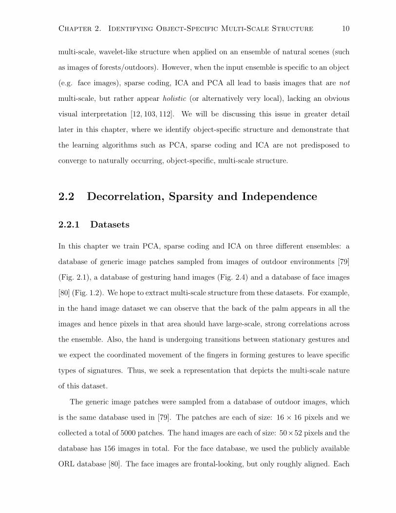
[80] (Fig. 1.2). We hope to extract multi-scale structure from these datasets. For example,
in the hand image dataset we can observe that the back of the palm appears in all the
images and hence pixels in that area should have large-scale, strong correlations across
the ensemble. Also, the hand is undergoing transitions between stationary gestures and
we expect the coordinated movement of the fingers in forming gestures to leave specific
types of signatures. Thus, we seek a representation that depicts the multi-scale nature
of this dataset.
The generic image patches were sampled from a database of outdoor images, which
is the same database used in [79]. The patches are each of size: 16 × 16 pixels and we
collected a total of 5000 patches. The hand images are each of size: 50×52 pixels and the
database has 156 images in total. For the face database, we used the publicly available
ORL database [80]. The face images are frontal-looking, but only roughly aligned. Each
Chapter 2. Identifying Object-Specific Multi-Scale Structure 11
Figure 2.4: Sample images from a database of a gesturing hand. Each sub-image is of
size: 50 × 52 pixels. The database contains images of 6 stationary gestures, and also
transition images between these gestures, for a total of 156 images.
image is of size: 112× 92 pixels and the database contains 400 images in total.
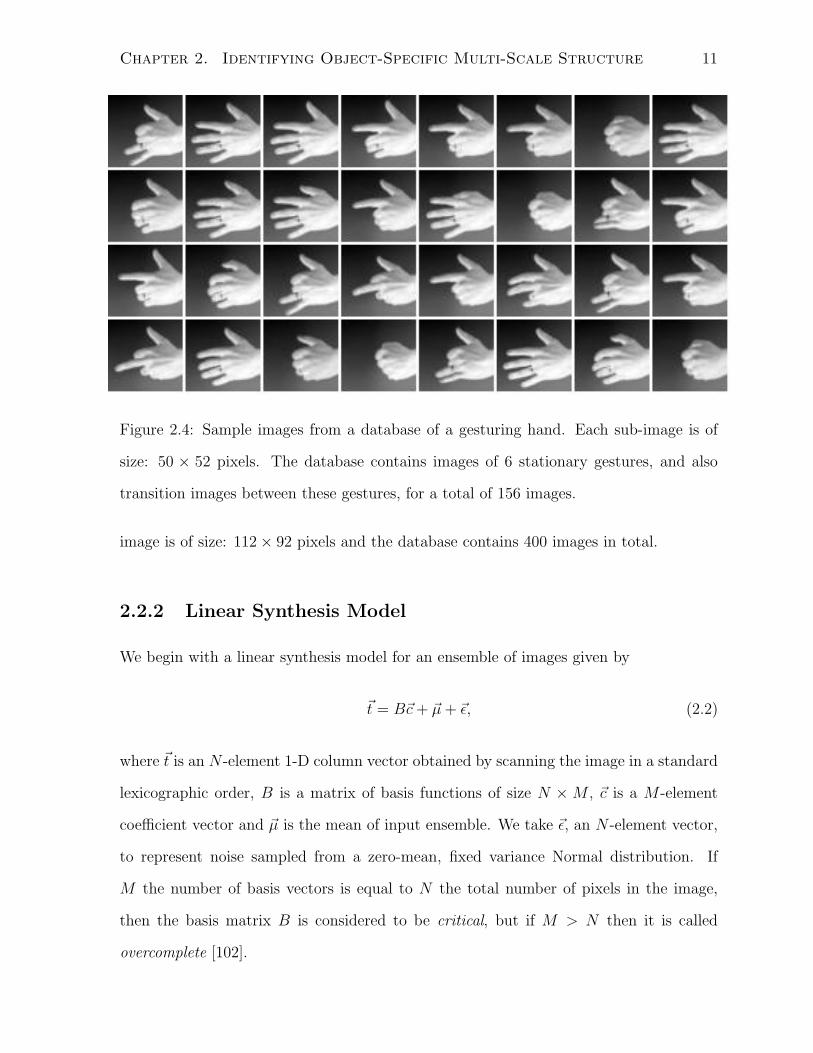
2.2.2 Linear Synthesis Model
We begin with a linear synthesis model for an ensemble of images given by
~t = B~c + ~µ + ~ε, (2.2)
where ~t is an N -element 1-D column vector obtained by scanning the image in a standard
lexicographic order, B is a matrix of basis functions of size N ×M , ~c is a M -element
coefficient vector and ~µ is the mean of input ensemble. We take ~ε, an N -element vector,
to represent noise sampled from a zero-mean, fixed variance Normal distribution. If
M the number of basis vectors is equal to N the total number of pixels in the image,
then the basis matrix B is considered to be critical, but if M > N then it is called
overcomplete [102].

Chapter 2. Identifying Object-Specific Multi-Scale Structure 12
2.2.3 Principal Component Analysis (PCA)
In PCA the goal is to construct a small set of basis functions (or images) that can
characterize the majority of the variation in the training set. We take the standard view
of PCA [49] (for a probabilistic treatment see [92,109]). Here the data is assumed to be
noise free (i.e., ~ε = 0) and the variation in the ensemble is characterized by the covariance
matrix S given by:
S = E[(~t− ~µ)(~t− ~µ)T
], (2.3)
where E represents the expectation over the image ensemble ~tkKk=1 and S is a matrix
of size N ×N . The eigenvectors of the covariance matrix given by
U =
[~u1 ~u2 · · · ~uN
]
form an orthonormal basis, that is
~uTk ~uj =
1 if k = j,
0 otherwise.
(2.4)
The eigenvectors satisfy
S~uj = σ2j~uj,
where σ2j is the eigenvalue denoting the variance of the input data projected onto the
basis direction ~uj and
σ21 ≥ σ2
2 · · · ≥ σ2n ≥ 0. (2.5)
In a matrix form
SU = UΣ, (2.6)
where Σ is a diagonal matrix with entries σ2j arranged on the diagonal according to
Eq. 2.5.
A low-dimensional representation for the input ensemble can be built if, for some M ,
the eigenvalues σ2k are small for k > M . In particular, using a principal subspace U

Chapter 2. Identifying Object-Specific Multi-Scale Structure 13
containing the leading M eigenvectors associated with the largest M eigenvalues of the
covariance matrix, namely
U =
[~u1 ~u2 · · · ~uM
], (2.7)
an approximation ~t can be made to the input image ~t,
~t = U~c + ~µ,
where the coefficient vector ~c is an M -element vector given by
~c = UT (~t− ~µ). (2.8)
There are two appealing properties to this eigenvector representation. One, for a
given sub-space dimensionality M , the principal subspace defined by the leading M -
eigenvectors is optimal in the sense of minimizing the mean squared reconstruction error
[49]:
E∥∥∥~t− ~t
∥∥∥2
,
where E stands for the expectation operator. Two, the basis matrix U leaves the output
coefficients decorrelated. In other words, the covariance matrix of the output coefficients
is the diagonal matrix Σ,
E[~c ~c T
]= Σ.
This equation can be easily derived by combining Eq. 2.8, 2.6 and 2.3.
Additionally, we introduce two quantities, one to describe the fraction of the total
input variance captured by a PCA basis image and the other to accumulate this fraction
over principal subspaces for a given dimensionality s. First, we denote the relative
variance captured by the mth basis vector to be dQm given by:
dQm =σ2
m∑Mk=1 σ2
k
. (2.9)
We use the variable−→dQ, a vector of length M , to represent the relative variances:
−→dQ =
[dQ1 dQ2 · · · dQM
], (2.10)
Chapter 2. Identifying Object-Specific Multi-Scale Structure 14
Second, we use Qs to represent the fraction of total variance a subspace of a given di-
mensionality s ≤M captures:
Qs =s∑
t=1
σ2t∑M
k=1 σ2k
,
=s∑
t=1
dQt. (2.11)
Similarly,−→Q is a M -element vector representing the cumulative variances of a M -
dimensional principal subspace:
−→Q =
[Q1 Q2 · · · QM
]. (2.12)
Results from PCA
Our goal here is to use PCA to assess the intrinsic dimensionality’s of the three image
ensembles mentioned in §2.2.1 and evaluate if the PCA bases appear to match our in-
tuition for object-specific structure. The datasets have been preprocessed to remove the
mean (as in Eq. 2.3) and an eigendecomposition is performed on the covariance matrix of
the mean-subtracted dataset. We then compute the relative variance−→dQ (Eq. 2.10) and
the cumulative variance−→Q (Eq. 2.12) separately for each one of the datasets. The plots
shown in Fig. 2.5 depict the variation in log (dQm) and Qm as we increase the subspace
dimensionality m.
For the face and hand image ensemble, the−→dQ plot shows eigen values dropping off
rapidly at first, then decreasing roughly exponentially (linearly in log (dQm) plot) for a
large range in the subspace dimension m. This we find is typical for a wide variety of
object-specific ensembles.
In comparison, for natural image ensembles we know the amplitude-spectrum has
a power law dependency on spatial frequency (Eq. 2.1). This effect can be seen in
the roughly linear fall-off that log (dQm) plot exhibits (up to m = 150 or so). It is
worth mentioning that the generic image patch dataset in [79] has been preprocessed by

Chapter 2. Identifying Object-Specific Multi-Scale Structure 15
50 100 150 200
−14
−12
−10
−8
−6
−4
m
log e(d
Q)
Natural Images : Relative Variance
0 50 100 1500
0.25
0.5
0.75
1
Q
m
Natural Images : Cumulative Variance
20 40 60 80 100 120 140
−11
−10
−9
−8
−7
−6
−5
−4
−3
−2
m
log e(d
Q)
Hands : Relative Variance
0 50 100 150 2000.3
0.4
0.5
0.6
0.7
0.8
0.9
1
Q
m
Hands : Cumulative Variance
50 100 150 200 250 300 350−9
−8
−7
−6
−5
−4
−3
−2
m
log e(d
Q)
Faces : Relative Variance
0 100 200 300 4000.1
0.2
0.3
0.4
0.5
0.6
0.7
0.8
0.9
1
Q
m
Faces : Cumulative Variance
(a) (b)
Figure 2.5: Plots of relative variance (a) and cumulative variance (b) for three different
datasets: (Top) Natural Images (Middle) Hand Images (Bottom) Face Images.

Chapter 2. Identifying Object-Specific Multi-Scale Structure 16
Figure 2.6: PCA basis for an ensemble of generic image patches. PCA basis are displayed
in the decreasing order of the input variance they capture, beginning at the top left corner
and going horizontally across the page. Observe that the fine-scale information captured
by the high-order eigenbasis is spread spatially across the entire image.
a combined low-pass/variance-adjusting filter in the frequency domain, first to remove
artifacts of rectangular sampling (that is to eliminate energies present in the corners of
the 2-D frequency domain) and then to reduce the effect of large inequities in variance
across frequency channels. The filtering effect can be seen in log(dQm) plot, where the
higher eigen bases report a sudden decrease in the accounted variance compared to what
the linear fall-off predicts.
From the Qm plot drawn for the generic image patch dataset, the first 50 bases
account for more than 70% of the mean-subtracted ensemble variance. However, for the
hand dataset, almost 95% of the variance is captured by a principal subspace of roughly
25 dimensions. The face database requires at least a 100 dimensional principal subspace
to account for 90% of the input variance.
The PCA basis vectors for a generic image patch ensemble are shown in Fig. 2.6. The

Chapter 2. Identifying Object-Specific Multi-Scale Structure 17
PCA basis look similar to a set of discrete Fourier harmonics and the reason is as follows
(see [38,70]). If image statistics are stationary and the covariance information is mainly
a function of the distance between pixels, then the covariance matrix exhibits a banded
symmetry. If the images are assumed to be periodic, then the covariance matrix takes on
a special form called a periodic Toeplitz matrix, where the elements along the diagonals
are constant. Interestingly, complex exponentials are eigenvectors of periodic Toeplitz
matrices. Hence, for generic image patches which have roughly stationary statistics, a
discrete Fourier basis is a good approximation to the PCA directions.
From Fig. 2.6 we can see that the PCA basis are global and spatial frequency-specific.
The leading eigenvectors appear to capture edge/line like structure at a coarse scale.
However, the remaining PCA basis are not simultaneously local in space and frequency.
Now we analyze the PCA basis images shown in Figs. 2.7 and 2.8, for the hand and the
face image ensembles, respectively. The first few basis vectors appear relatively smooth
and hence they represent global correlations. In particular, for small values of the eigen
vector index m the basis images seem to depict larger scales. An approximate measure
of the scale, and hence the correlation length, can be inferred by estimating the size of
a blob of one sign (either positive or negative) appearing in a basis image. As the index
m for the principal component increases, the scale gets finer and hence the basis vectors
appear to represent fine scale structure. However, they remain global in space. This
clearly is not representative of the object-specific local structure that we believe these
images to possess.
2.2.4 Sparse Coding and ICA
The goal in sparse coding is to seek a linear basis representation where each image
is represented by a small number of active coefficients (e.g. [38, 46, 79]). The learning
algorithm involves adapting a basis vector set, while imposing a low-entropy (or sparse)
prior on the output coefficients. One example of a low-entropy prior is the double-sided

Chapter 2. Identifying Object-Specific Multi-Scale Structure 18
Figure 2.7: PCA results on the hand images. PCA basis are displayed in the decreasing
order of the input variance they capture, beginning at the top left corner and going
horizontally across the page. Note, fine-scale information represented by the high-order
eigenvectors is spread across the entire image.
Laplacian,
p(cj) ∝ exp(−∣∣∣cj
θ
∣∣∣)
, (2.13)
where p(cj) is the probability distribution on the jth element of an output coefficient
vector ~c. For a discussion on low-entropy priors suitable for sparse coding see [46, 79].
Typically, these are uni-modal, long-tailed distributions with significant probability mass
around the origin and having high-kurtosis.
The intuition for sparse priors comes from analyzing the statistics of natural scenes. In
particular, evidence for sparse structure can be seen by processing images with wavelet-
type filters (Fig. 2.2) and studying the histogram of the filter coefficients. It is clear
from the wavelet processed image shown in Fig. 2.3 that smooth regions in an image
typically provide negligible filter coefficients. But transition regions, e.g. image patches
that appear line-like locally, and in the case of Fig. 2.3 oriented 90 degrees away from the
horizontal, have high magnitudes. The resulting filter coefficient histograms show high
kurtosis, which is taken to indicate sparse structure.
On the contrary, if the same image structure is filtered with global fine scale PCA

Chapter 2. Identifying Object-Specific Multi-Scale Structure 19
Figure 2.8: PCA basis vectors on face images from the ORL database [80]. The first 40
principal components are displayed in the decreasing order of the input variance they
capture, beginning at the top left corner and going horizontally across the page. Observe
the finer-scale information represented by the higher-order eigenvectors is spread across
the entire image.

Chapter 2. Identifying Object-Specific Multi-Scale Structure 20
basis, then the coefficient histograms are more nearly Gaussian. This effect is due to the
Central Limit Theorem, for which the sum of a larger number of independent random
variables each of finite variance is approximately Gaussian, no matter what their individ-
ual distributions are. So, the hope in using a low-entropy prior for the coefficients is that
the adapted basis vector set will acquire the shape and form of the naturally-occurring
multi-scale structure.
For a given image ensemble~ti
i=1..pa sparse representation is learned by minimizing
the following cost function [46,79]:
E(λ) =∑
i
Ei(λ) =∑
i
[||~ti −B~ci||22 + λ
∑
j
Ω(cij)
]. (2.14)
The cost function Ei(λ) for each image ~ti contains two terms: a reconstruction error term
given by ||~ti−B~ci||22 and a regularization term given by λ∑
j Ω(cij). The reconstruction
error term encourages B to span the subspace containing the input vectors~ti
i=1..p.
The regularization term is set up to favor solutions in which the responses cij match
the prespecified prior distribution on the coefficients. In particular, the prior on the
coefficients is assumed to be statistically independent, that is,
p(~c) =∏
j
p(cj). (2.15)
Then the penalty term Ω(cj) can be expressed as
Ω(cj) = log (p(cj)) . (2.16)
The regularization parameter λ controls the weighting of the prior term in the cost
function.
The overall cost function E(λ) is minimized in two stages. In the inner loop for
each image ~ti, the basis matrix B is held fixed and Ei(λ) is minimized with respect to
the coefficient vector ~ci. In the outer loop, after coding several training images, the
accumulated E(λ) is minimized with respect to B. The regularization parameter λ need
not be held fixed [79].

Chapter 2. Identifying Object-Specific Multi-Scale Structure 21
Before initiating the sparse coding procedure, several decisions have to be made:
choosing a functional form for the low-entropy prior (Eq. 2.16,2.13), fixing an appropriate
value for λ or deciding to learn it from the data, and guessing a lower bound on the number
of basis vectors needed to extract independent components in the images (Eq. 2.14). Our
implementation follows the improved version of the sparse coding algorithm presented
in [60].
Independent Component Analysis (ICA) is an algorithm based on maximizing the
mutual information between the inputs and outputs of an information processing network
[13]. ICA can be understood as solving a maximum-likelihood problem, similar to the
one posed by sparse coding [67,79,83]. In particular, there are two assumptions made in
ICA: the ensemble is assumed to be noise-free (~ε = 0) and the basis matrix has a critical
form where the number of basis vectors M is equal to the number of pixels N in the
input image. Because the basis matrix is critical and the noise is zero, the reconstruction
error term in Eq. 2.14 is also zero as long as the basis matrix is linearly independent.
This leads to a simple formulation for the optimal basis:
B† = arg minB
[λ∑
i
∑
j
Ω([B−1~ti]j
)− log| det(B−1) |
]. (2.17)
Instead of adapting the basis matrix B, in the ICA formulation a filter matrix D is
learned, where
D = B−1. (2.18)
The rows of D act as filters and the filter coefficients are obtained by applying the filter
matrix to the image ~t:
~c = D~t. (2.19)
The learning formulation specified in Eq. 2.17 for the optimal basis matrix B can be easily
rewritten to obtain update equations for an optimal filter matrix D. This is precisely
the formulation given in the ICA algorithm [13], under the condition that the output of

Chapter 2. Identifying Object-Specific Multi-Scale Structure 22
the ICA network be equal to the cumulative density function of the sparse prior on the
coefficients.
As argued in [13] maximizing the mutual information between the inputs and outputs
of an information processing network promotes independence in the distribution of the
output coefficients. However, a transformation that minimizes the entropy of the indi-
vidual outputs also promotes their statistical independence (see [46] or Sec 2.5 in [45]).
To get a better understanding of this issue, consider the mutual information I(~c ; ~t
)
between the output ~c and input ~t of an information processing system. We will assume
the dimensionalities of the input signal ~t and the output coefficient ~c are the same. The
mutual information I(~c ; ~t
)can be written as the difference between the joint entropy
of the output coefficients H (~c) and the conditional entropy of the output given the input
given by H (~c | ~x). If the system is assumed to be noiseless, then the conditional entropy
in the output given the input H (~c | ~x) is zero. In this case, maximizing the mutual
information between the input and output is equivalent to maximizing the overall output
entropy. Furthermore, the output entropy is given by the sum of the individual output
element entropies minus any mutual information between them:
H(~c) =∑
i
H(ai)−∑
i
I(ci; ci−1, · · · , c1)
. In attempting to maximize the output entropy, we can simultaneously minimize the
mutual information term if the individual entropies∑
i H(ai) are suitably constrained,
either by applying some upper bound or by placing a downward pressure on the sum
of the output entropies, as is done in low-entropy or sparse coding. In this way, the
mutual information between the output elements is reduced, thus promoting statistical
independence among outputs. In fact, in much of the literature the term “independent”,
as applied to the study of low-level structure in images, is abused when they really mean
“low-entropy” (e.g., [14]). We continue this tradition when we refer to the “independent
components”.

Chapter 2. Identifying Object-Specific Multi-Scale Structure 23
Results from Sparse Coding
The strategies of sparse coding and ICA were deemed successful because they extract
multi-scale, wavelet-like structure when applied to an ensemble of natural scenes (such as
the images from outdoors/forests) [14,46,79]. This result was seen to be insensitive to the
exact functional form of the low-entropy prior [46, 79]. However, for object-specific en-
sembles we observe that it can be difficult to extract object-specific structure by imposing
a low-entropy prior on the output coefficients.
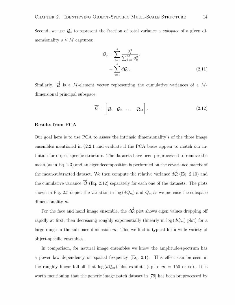
In Figures 2.9 and 2.10 we show results of sparse coding on the hand image dataset.
As shown in Fig. 2.5, this ensemble has a low-dimensional description in that the eigen
spectrum decays rapidly. So we assume independent components, if any, will reside
within a low-dimensional sub-space. Our experience with sparse coding suggests that
this procedure has difficulty finding the correct low-dimensional subspace and resolving
the independent components within [23]. During optimization, perturbations to the
basis matrix B will cause the representation to move away from the spanning space.
Optimization steps mainly cause the updates to move the basis matrix B to the spanning
space, instead of modifying the representation so it can come closer to capturing the
structure within the spanning space. Assuming this to be the case, we split the problem
into two sub-problems, namely the restriction to the subspace and the representation
within the subspace.
The restriction to the subspace is achieved by principal component analysis (PCA).
Images are projected to a low-dimensional subspace spanned by an orthogonal set of
principal component vectors:
~q = UT~t,
where ~t is the input image, U is a basis matrix with a small number of principal compo-
nents, UT is the PCA matrix transposed and ~q is the resulting low-dimensional coefficient

Chapter 2. Identifying Object-Specific Multi-Scale Structure 24
vector. We then search for the sparse structure matrix B ′ in the projected space:
~q = B′~c,
where a low-entropy prior is placed on ~c and B ′ resolves the sparse structure in the set
of low-dimensional data points ~q. These two equations can be combined to give the
independent components matrix B:
~t = U~q,
= UB′~c,
= B~c.
So to facilitate sparse coding, we first project the data into the space spanned by
the first 10 principal components. We can see from Fig. 2.5 that the first ten principal
components account for more than 90% of the input variance. However, in this 10-
dimensional principal subspace it is not clear how many independent components one
should search for. Recall in the sparse coding framework we have the freedom to set
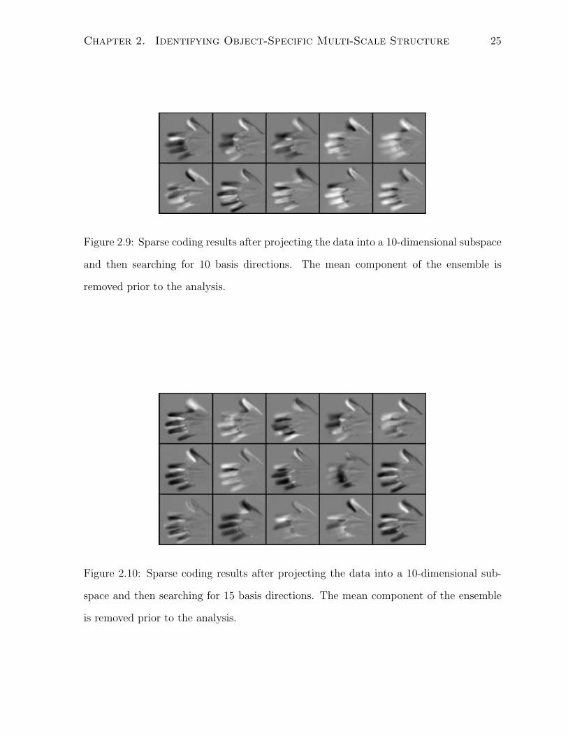
the basis matrix to be overcomplete. In Figures 2.9 and 2.10 we show the results from
extracting 10 and 15 independent components respectively. The overall appearance of the
basis vectors is global and edge-like (alternating dark and bright regions). They cannot
be simply interpreted in terms of object parts, i.e. fingers of a hand. We also applied
the ICA algorithm in [13] but the results are not very different from the ones shown for
sparse coding.
For sparse coding/ICA results on the face images the reader is referred to the thesis
in [12], where the filter matrix shows some resemblance to facial features, but the resulting
basis matrix appears “holistic”. Thus, we have demonstrated that PCA, sparse coding
and ICA do not necessarily extract object-specific, multi-scale, local structure. Either our
intuition is wrong and the datasets do not contain such structure or the three algorithms
have failed to extract it. We next turn our attention to characterizing object-specific
structure and discuss how this may impose novel constraints on a learning algorithm.
Chapter 2. Identifying Object-Specific Multi-Scale Structure 25
Figure 2.9: Sparse coding results after projecting the data into a 10-dimensional subspace
and then searching for 10 basis directions. The mean component of the ensemble is
removed prior to the analysis.
Figure 2.10: Sparse coding results after projecting the data into a 10-dimensional sub-
space and then searching for 15 basis directions. The mean component of the ensemble
is removed prior to the analysis.
Chapter 2. Identifying Object-Specific Multi-Scale Structure 26
2.3 Object-Specific Multi-Scale Structure
What is the structure one can expect to find in an object-specific ensemble? We show
that object-specific ensembles exhibit structure in a low-dimensional subspace in a sparse,
scale-dependent, local form. In particular, there is large-scale structure correlated across
the entire image and fine-scale structure that is spatially localized. Although we study
a database of gesturing hand images (Fig. 2.4), the following argument holds true for
other object-specific ensembles as well. Once the structure is made explicit, it is easier
to conclude whether PCA, sparse coding or ICA was successful in extracting the object-
specific structure.
We review the observations made by Penev and Atick in [85]. Here we extend their
results to highlight object-specific multi-scale properties. We begin with a linear low-
dimensional representation for the ensemble, which can be readily obtained by PCA.
As we discussed earlier, the principal components characterize the second-order statis-
tical variation in the ensemble. The associated variance spectrum, for a majority of
object-specific ensembles, shows a rapid drop at first, then starts to decrease roughly
exponentially (Fig. 2.5). The images in the ensemble can be approximated using a small
number of principal components.
We assume each input image ~t that is N -pixels long is approximated by M leading
principal components to give:
~t = U1:MUT1:M
~t, (2.20)
where U is the principal component matrix spanning the image space, U1:M is a sub-
matrix with M leading principal components and M << N , the size of the input image.
Notice that U1:MUT1:M is the projection/reconstruction operator for the M -dimensional
subspace approximating the image ensemble.
To understand structure, we ask what it means to reconstruct the intensity at a
pixel position r in ~t? It involves the rth row of the projection operator: U1:MUT1:M . We

Chapter 2. Identifying Object-Specific Multi-Scale Structure 27
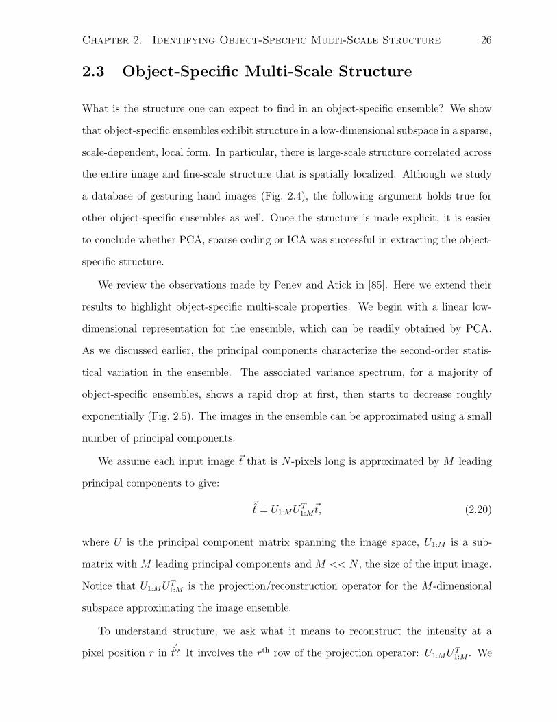
rearrange the data in the rth row of the matrix U1:MUT1:M , so it can be seen as an image
of the same size as the input. As we show in Fig. 2.11, the rth row of U1:MUT1:M varies
with M . Observe that with increasing M , the appearance of the rth row changes from
being global to very local. We interpret the projection operator in the following way:
• U1:MUT1:M captures correlations, not in the raw image space, but in the whitened
space. For each image ~t there is a whitened image ~j given by:
~j = U1:MΣ−1/2UT1:M
~t,
= U1:MΣ−1/2~q,
= U1:M~d,
where ~q = UT1:M
~t is the vector of PCA coefficients for input image ~t, Σ is a diagonal
matrix providing the variance in each element of the coefficient vector ~q across
the ensemble, and ~d is a rescaling of ~q such that it can be treated as a sample
from a zero-mean unit-variance Gaussian distribution (assuming the dataset is zero
mean). The image ~j is considered whitened because the covariance matrix of ~d is
the identity matrix. Hence, the covariance of the whitened image ensemble is given
by:
< ~j~jT > = U1:M < ~d~dT > UT1:M ,
= U1:MUT1:M .
• The correlation in the space of whitened images < ~j~jT > provides a measure of how
appropriate it was to use M global models in representing the image ensemble. If
the correlations are large, global models such as PCA are appropriate. Otherwise,
at least some spatially local models (and perhaps some global models) would be
more appropriate. This is clearly the case for M = 12 and higher in Fig. 2.11.
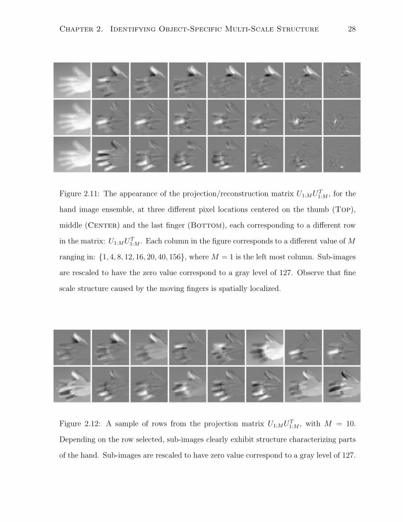
In Fig. 2.12 we show how the correlation map at each pixel appears to have a shape,
characteristic of a part of the object (i.e. the hand and its fingers) and the correlation
Chapter 2. Identifying Object-Specific Multi-Scale Structure 28
Figure 2.11: The appearance of the projection/reconstruction matrix U1:MUT1:M , for the
hand image ensemble, at three different pixel locations centered on the thumb (Top),
middle (Center) and the last finger (Bottom), each corresponding to a different row
in the matrix: U1:MUT1:M . Each column in the figure corresponds to a different value of M
ranging in: 1, 4, 8, 12, 16, 20, 40, 156, where M = 1 is the left most column. Sub-images
are rescaled to have the zero value correspond to a gray level of 127. Observe that fine
scale structure caused by the moving fingers is spatially localized.
Figure 2.12: A sample of rows from the projection matrix U1:MUT1:M , with M = 10.
Depending on the row selected, sub-images clearly exhibit structure characterizing parts
of the hand. Sub-images are rescaled to have zero value correspond to a gray level of 127.
Chapter 2. Identifying Object-Specific Multi-Scale Structure 29
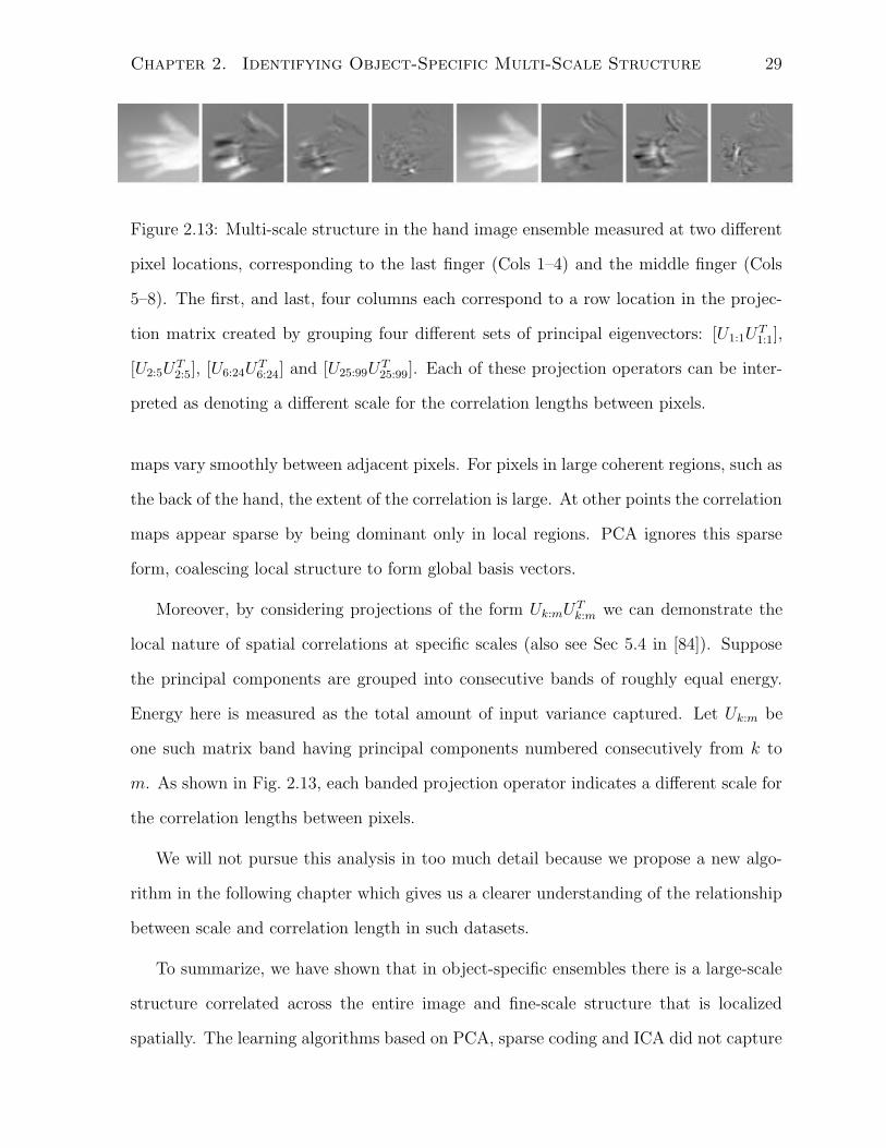
Figure 2.13: Multi-scale structure in the hand image ensemble measured at two different
pixel locations, corresponding to the last finger (Cols 1–4) and the middle finger (Cols
5–8). The first, and last, four columns each correspond to a row location in the projec-
tion matrix created by grouping four different sets of principal eigenvectors: [U1:1UT1:1],
[U2:5UT2:5], [U6:24U
T6:24] and [U25:99U
T25:99]. Each of these projection operators can be inter-
preted as denoting a different scale for the correlation lengths between pixels.
maps vary smoothly between adjacent pixels. For pixels in large coherent regions, such as
the back of the hand, the extent of the correlation is large. At other points the correlation
maps appear sparse by being dominant only in local regions. PCA ignores this sparse
form, coalescing local structure to form global basis vectors.
Moreover, by considering projections of the form Uk:mUTk:m we can demonstrate the
local nature of spatial correlations at specific scales (also see Sec 5.4 in [84]). Suppose
the principal components are grouped into consecutive bands of roughly equal energy.
Energy here is measured as the total amount of input variance captured. Let Uk:m be
one such matrix band having principal components numbered consecutively from k to
m. As shown in Fig. 2.13, each banded projection operator indicates a different scale for
the correlation lengths between pixels.
We will not pursue this analysis in too much detail because we propose a new algo-
rithm in the following chapter which gives us a clearer understanding of the relationship
between scale and correlation length in such datasets.
To summarize, we have shown that in object-specific ensembles there is a large-scale
structure correlated across the entire image and fine-scale structure that is localized
spatially. The learning algorithms based on PCA, sparse coding and ICA did not capture

Chapter 2. Identifying Object-Specific Multi-Scale Structure 30
this structure. As we demonstrate in the next chapter, placing a sparse prior on the
basis elements, instead of output coefficients, is a powerful way to predispose a learning
mechanism to converge to this naturally-occurring, sparse, multi-scale, local structure.
In particular, we demonstrate that when eigenvalues are pooled into bands of roughly
equal values, the corresponding eigenvectors within each band possess many rotational
degrees of freedom that can be utilized.

Chapter 3
Sparse Principal Component
Analysis: S-PCA
3.1 Introduction
A primary contribution of this thesis is to show how multi-scale representations emerge,
for a variety of image ensembles, by trading off redundancy minimization for sparsity
maximization in a basis matrix. We base our strategy Sparse Principal Component
Analysis (S-PCA) on the observation we made in the previous chapter, that natural
images exhibit structure in a low-dimensional subspace in a sparse, scale-dependent form.
S-PCA learns an orthonormal basis by rotating the basis vectors that span the principal
subspace. Rotation achieves sparsity in the basis vectors at the cost of introducing
small correlations in the output coefficients. If the input ensemble is a multi-dimensional
Gaussian with widely separated variance distribution (that is the ratio of successive values
in the eigen spectrum is large) , then S-PCA returns a redundancy minimizing solution,
namely the basis vectors of PCA. On the other hand, if the input ensemble is devoid
of any structure (i.e. i.i.d. pixel intensities), then S-PCA returns a maximally sparse
representation, with each basis vector representing the brightness at a single pixel. As
31

Chapter 3. Sparse Principal Component Analysis: S-PCA 32
our examples show, this property of returning a sparse representation, when possible,
provides a much more intuitive representation of the ensemble than a standard PCA
based representation.
Besides this theoretical advantage of providing a better intuitive model of an ensemble,
the computation of the basis coefficients is more efficient because of the presence of zero
valued weights in the sparse basis vectors. The speed-up obtained from this sparsity will
depend on both the ensemble and on the number of basis vectors used. In particular,
for all the natural data sets we have considered, the S-PCA basis vectors tend to get
increasingly sparse as the corresponding variances decrease. Therefore the speed-up due
to sparsity can be very significant when many basis vectors are used, but less significant
when only a few are used.
3.2 Encouraging Sparsity
To illustrate the basic idea of S-PCA, consider 2-pixel image ensembles generated from a
multi-dimensional Gaussian distribution. Each image is a point in a 2-dimensional space.
In Fig. 3.1, we show two such datasets, one with a dominant orientation (a) and the other
essentially isotropic (b).
PCA determines an orthonormal set of basis vectors with the property that the basis
expansion coefficients are decorrelated. The idea of PCA in this 2D example is to rotate
the pixel basis, [ 1 00 1 ], until the variance of the projected data is maximized for one compo-
nent and is minimized for the other. In Fig. 3.1, the PCA directions for the distributions
are shown in blue. For the correlated dataset in Fig. 3.1a, the PCA vectors are aligned
with the oriented structure underneath. For the uncorrelated dataset in Fig. 3.1b, the
specific directions that PCA selects are dictated by sampling noise. For such datasets
we prefer basis vectors that are sparse (and orthonormal), that is, have few non-zero
entries. In this 2D example, this is just the pixel basis, [ 1 00 1 ], as shown in red in Fig. 3.1b.

Chapter 3. Sparse Principal Component Analysis: S-PCA 33
−4 −2 0 2 4−4
−2
0
2
4
Pixel 1
Pix
el 2
Distribution 2
−20 0 20−20
−10
0
10
20
Pixel 1
Pix
el 2
Distribution 1
(a) (b)
Figure 3.1: What is PCA good for? Distributions 1 and 2 (black dots) are 2-pixel
image ensembles sampled from multi-dimensional Gaussian priors. (a) Distribution 1
has a dominant orientation indicated by the PCA basis (blue). (b) Distribution 2 has
no orientational structure, and the PCA basis (blue) reflects sampling noise. In both
cases the preferred S-PCA basis vectors are obtained by rotating PCA directions. In (a)
the rotation is minimal, while in (b) the rotation maximizes sparsity in the basis vector
description by aligning them with the pixel basis.
Note the sparse basis can be achieved by simply rotating the PCA basis by an amount
depending on the degree of correlation in the underlying dataset.
3.3 S-PCA Pairwise Rotation Algorithm
The idea behind S-PCA is to retain the PCA directions when there is correlational
structure in the data set, and otherwise rotate them to be as sparse as possible. We
propose a cost function
C(λ) = C1 + λC2, (3.1)

Chapter 3. Sparse Principal Component Analysis: S-PCA 34
where C1 is a function of the variances of the data projected onto the individual basis
vectors, and C2 is a function of the elements of the basis vectors themselves. The exact
form for C1 and C2 are not so important, so long as C1 is designed to retain the PCA
directions while C2 promotes sparsity. The λ parameter in the cost function provides
the relative importance of the sparsity term, and we choose it to make the contributions
from C1 and C2 have the same scale. See the next section for the actual forms of C1, C2
and how λ was selected to keep the scale of C1 and C2 the same in all the examples used
in this thesis.
The learning algorithm of S-PCA is very simple. The basis vectors are initialized to be
the principal components or any other convenient orthonormal basis. The dimensionality
of this principal subspace is chosen beforehand. Selecting a maximal dimension basis is
also possible. Every pair of these basis vectors defines a hyperplane, and we successively
select suitable rotations within these hyperplanes to minimize C(λ). We sweep through
every possible basis vector pair doing these rotations, and these sweeps are repeated until
the change in C(λ) is below a threshold. The product of the pairwise rotations provides
a composite rotation matrix which, when applied to the PCA vectors generates the S-
PCA basis. In particular, the S-PCA and PCA bases are orthonormal representations
for the same subspace and are related to each by other by this rotation matrix. A typical
implementation of this algorithm is given in the next section.
The PCA basis is used as the starting point since it identifies the principal subspace
best suited to recovering correlational structure. The job of the S-PCA algorithm is then
simply to resolve the range of the spatial correlations. Note that the S-PCA basis is
always a rotation of the original basis, so some care should be taken in choosing this
starting basis. In cases for which we want a complete representation (that is the basis
matrix is square), we have found that the trivial basis (i.e. provided by the columns of
an identity matrix), and also random orthonormal matrices, can be used as a starting
point for the S-PCA algorithm.
Chapter 3. Sparse Principal Component Analysis: S-PCA 35
3.3.1 Details
A typical implementation of S-PCA is given in Algorithm 1. We chose a entropy-like
measure for the two terms C1 and C2 in the cost function. It is also possible to have a
probabilistic treatment for the cost function, and we present this in a later chapter.
Let U =[~u1 ~u2 · · · ~uM
]be a basis matrix spanning an M−dimensional subspace,
with ~um =(u1,m, . . . , uN,m
)Tand ~uT
m~uk = δm,k (the Kronecker delta). Let σ2m be the
variance of the data projected onto the direction ~um. Using Eq. 2.10 we set up a relative
variance vector
−→dQ =
[dQ1 dQ2 · · · dQM
]
where
dQm =σ2
m∑Mk=1 σ2
k
.
The first term of the cost function, namely C1
(−→dQ), is defined as
C1
(−→dQ)
=M∑
m=1
−dQm log(dQm). (3.2)
It can be shown that C1
(−→dQ ; U
)is minimized if and only if the basis vectors U are
PCA directions [32].
The second term in the cost function, namely C2(U), is defined as
C2(U) =M∑
m=1
N∑
n=1
−u2n,m log(u2
n,m). (3.3)
Notice that this is just the sum of the entropies of the distributions defined by the square
of the elements for each basis vector ~um (recall the basis vectors have unit norm). If
the elements of the basis vector have a Gaussian-like distribution, as in PCA, entropy
is high and so is the cost function C2. If the basis vectors form an identity matrix,
entropy is minimal, i.e. zero. Thus, C2(U) promotes sparsity. We have also experi-
mented with other concave objective functions that can promote sparsity in C2(U), e.g.
∑mn log [α + β exp (− |un,m/γ|)] where α, β and γ are the parameters of the sparsity
driving function, and observed qualitatively similar results with S-PCA.

Chapter 3. Sparse Principal Component Analysis: S-PCA 36
We choose the λ parameter such that the contributions from C1 and C2 to the overall
cost function C will be on the same scale. For this we need to know the range of values
C1 and C2 take for a typical dataset. For example, the cost term C2 is a function of the
elements of the basis vectors (Eq. 3.3) and is independent of any other properties of the
input data. In particular, for an identity basis (or any permutation thereof), which is
the sparsest matrix, the contribution from C2 is 0, but for an orthonormal matrix of size
N ×M having entries each of size 1/√
N , C2 contributes a maximum value of M log(N).
Similarly, the term C1 measures the entropy of a variance distribution (Eq. 3.2). The
entropy is minimal when the basis vectors are PCA directions and maximal if the variance
is spread uniformly across all the basis directions. The upper-bound is clearly log(M)
but how do we get an estimate for the lower-bound set by the PCA basis? One simple
approach is to assume scale-invariant statistics in the dataset (Fig. 2.5 Top) where the
power spectrum is inversely proportional to the square of the spatial frequency Eq. 2.1.
Following the discussion in §2.2.3, we can replace the spatial frequency index f in Eq. 2.1
by the eigenbasis index m and develop an analytical form for the variance spectrum:
σ2m ∝ 1/m2.
We use this expression to empirically evaluate C1 for various values of M , the dimen-
sionality of the principal subspace. With increasing M , the maximum value C1 can take
changes as log(M) but we observe a much slower growth in the lower-bound, with C1
approaching an asymptotic value of 2.3626. Also, from the analysis presented in Fig. 3.1
we expect the variance spectrum returned by S-PCA basis to be ’close’ to the spectrum
obtained by PCA directions. In fact we show this to be the case for a wide variety of en-
sembles. Thus it makes sense to set a value for λ that scales C2 to match the lower-bound
of C1. We use the following expression for λ for all the datasets used in this thesis:
1
λ= M log(N). (3.4)
In choosing λ we have ignored the size of the dataset, which obviously affects the com-

Chapter 3. Sparse Principal Component Analysis: S-PCA 37
putation of the variance spectrum. Also, not all datasets have scale-invariant statistics
and we may have to adjust the λ parameter accordingly.
Additionally, there are two implementation details that are worth mentioning. First,
the optimization problem reduces to a sequence of rotations involving pairs of basis
vectors, [ui uj]. One trick is to not consider every basis pair. For example, if the variances
on the corresponding basis pair are widely different, then they are likely to correspond to
the situation shown in Fig. 3.1a. In this case, there should be no significant rotation. A
simple way to disregard a basis pair [ui uj] is to check if the log ratio of the corresponding
variances: max(σ2
i , σ2j
)/min
(σ2
i , σ2j
), is less than a threshold. We use a threshold of 7.0
on all the datasets reported in this thesis. However, we found S-PCA results not to be
overly sensitive to the actual setting of this threshold. Secondly, there is a search done
for the correct rotation angle θij. The gradient of the cost function with respect to the
rotation angle θij is easy to derive and hence, can be used while searching for the optimal
solution. However, we find the results are as good if we take the less expensive option,
which is to use optimization routines that do not use gradient information (eg. routines
mnbrak in conjunction with brent from [89]).
As we discuss next, the iterative algorithm converges to a stationary point of the cost
function C(λ). We select a basis pair and search for a suitable rotation in the hyperplane
defined by the basis pair that minimizes C(λ). Because the rotation is within the hy-
perplane, contribution to the overall cost function C(λ) by the remaining basis vectors,
and their variances, does not change. We use this fact in setting up the optimization
problem (Algorithm 1, lines 16 − 18). Because the rotation angle, selected for every
basis pair, minimizes the cost function, and a rotation update to the basis directions, and
the corresponding variances, is applied before picking the next basis pair (Algorithm 1,
lines 19 − 20), the algorithm either continuously descends or remains stationary. Thus,
at the end of every sweep the overall cost function has either been reduced or is left at a
stationary point.

Chapter 3. Sparse Principal Component Analysis: S-PCA 38
Algorithm 1 Function U = Sparse-PCA(U, Σ, λ)
1: INPUT
2: U ⇐ U is a N ×M matrix with orthonormal columns, M ≤ N
3: Σ⇐ Variance matrix for data projected onto U : Σii = σ2i ; Σij = Σji = σ2
ij
4: λ⇐ Sparsity factor which can be a function of N and M as in Eq. 3.4
5: OUTPUT
6: U ⇐ Sparse PCA basis matrix
7: CONSTANTS
8: θinit = 0; θtol = 1.0e−4; ε = 1.0e−8
9:
10: dm =σ2
m∑Mk=1 σ2
k
∀m = 1 · · ·M ; ~d =(d1, . . . , dM
)T
11: Cnew = C1(~d) + λC2(U) Eq. 3.2 and 3.3
12: while not converged do
13: Cold = Cnew
14: for i = 1 to M -1 do
15: for j = i + 1 to M do
16: U ⇐[~ui ~uj
]; D ⇐
[ σ2i∑M
k=1σ2
k
σ2ij∑M
k=1σ2
k
σ2ij∑M
k=1σ2
k
σ2j∑M
k=1σ2
k
]
17: θij = θinit; R(θij) =
[cos(θij) − sin(θij)
sin(θij) cos(θij)
]
18: θij ⇐ MINIMIZE
C1
(diag(RT DR)
)+ λC2
(UR
)for θij
19: U(:, [i j]
)= UR(θij) if θij > θtol Update the i and j columns of U
20:
(σ2
i σ2ij
σ2ji σ2
j
)= R(θij)
T
(σ2
i σ2ij
σ2ji σ2
j
)R(θij) if θij > θtol Update entries in Σ
21: end for
22: end for
23: Cnew = C1(~d) + λC2(U) Compute ~d as in Line 10 above (Eq. 3.1)
24: converged =(∣∣∣Cold−Cnew
Cold
∣∣∣ < ε)
25: end while

Chapter 3. Sparse Principal Component Analysis: S-PCA 39
3.4 S-PCA on Datasets With Known Structure
We demonstrate results from applying S-PCA on datasets where the structure is known
a priori. Consider an image ensemble generated by convolving Gaussian white-noise
vectors with a filter kernel and adding small amounts of noise to the filtered signals
(Fig. 3.2). The generative model can be written as:
~y = ~g ⊗ ~x + κ~n, (3.5)
where ~x and ~n are samples from a zero-mean, unit-variance Gaussian distribution, ⊗ is
the convolution operator, ~g is a filter kernel, ~y is the noisy version of the filtered signal
~g ⊗ ~x and finally, κ is the standard deviation of the noise distribution chosen to be 2%
of the maximum absolute value in the ensemble. This translates to about 5 gray levels
for an image with a peak intensity value of 255 gray levels. In Fig. 3.2(a & b) we also
show the filter kernels which are low-pass and band-pass respectively. The filters are
modeled after a Gaussian function and its second derivative. The standard deviation of
the Gaussian was chosen to be 1 pixel and the filters were designed to be 7-tap long. The
ensemble contains 10000 samples of the filtered signal ~y.
3.4.1 Low-Pass Filtered Noise Ensemble
We begin our analysis with a low-pass filtered noise ensemble. We expect to see corre-
lations in spatially local neighborhoods of the output signal ~y because of the Gaussian
smoothing. We now show that S-PCA provides a representation which highlights this
structure.
A Principal Component Analysis (PCA) of such a data set provides a basis represen-
tation which is global and spatial frequency specific. The PCA basis vectors are shown
in Fig. 3.3 and a Fourier transform of each individual basis vector is shown in Fig. 3.4.
The variance spectrum resulting from the PCA basis is shown in Fig. 3.7. Notice that

Chapter 3. Sparse Principal Component Analysis: S-PCA 40
5 10 15 20 25 30
−1.5
−1
−0.5
0
0.5
1
1.5
n
x(n)
, y(n
)
5 10 15 20 25 30−2
−1.5
−1
−0.5
0
0.5
1
1.5
2
n
x(n)
, y(n
)
5 10 15 20 25 30−0.5
0
0.5
1
1.5
2
2.5
n
x(n)
, y(n
)
Figure 3.2: (Left & Middle) Stem plots in blue are Gaussian noise signals, which
are filtered by a low-pass kernel (drawn as an inset figure (Left)) and a band-pass
kernel (also drawn as an inset figure (Middle)). The filtered signals are shown in green
and their noisy versions are drawn in red. (Right) Noisy versions of sine waves each
initialized with a random phase/amplitude and a random DC value. Signals are 32 pixel
long vectors.
the PCA representation does not highlight the spatially localized structure introduced
by Gaussian smoothing.
In comparison, the S-PCA basis derived for the low-pass filtered noise ensemble pro-
vides structure at multiple scales, evident from the spatial domain plot in Fig. 3.3 and the
frequency domain plot in Fig. 3.4. The first few basis vectors appear as low-pass filters in
the spatial domain, whose size is indicative of the Gaussian kernel used to introduce the
correlations between pixels. While these basis vectors are spread evenly over the pixel
space, they cannot significantly overlap due to the orthogonality constraint. Instead,
basis vectors at the next scale exhibit entries with multiple signs, but still remain local.
To confirm if there is a good match between the correlation lengths depicted by the
multi-scale basis vectors and the scale of the low-pass kernel used to generate the ensemble
(Fig. 3.2), we overlay a (circularly) shifted and scaled version of the low-pass kernel on
each of the S-PCA basis vectors as shown in Fig. 3.5. Visually, the scales appear to be
in good agreement and we confirm this numerically by computing a scale value for each

Chapter 3. Sparse Principal Component Analysis: S-PCA 41
PCA
S-PCA
Figure 3.3: Representing Gaussian filtered noise ensemble using PCA (Top) and S-PCA
(Bottom). Each waveform is 32 pixels long. In each waveform the zero line is near the
median value of the waveform. Zero valued weights in S-PCA results indicate a sparse
basis matrix.

Chapter 3. Sparse Principal Component Analysis: S-PCA 42
PCA Basis in Fourier Domain
S-PCA Basis in Fourier Domain
Figure 3.4: Representing Gaussian filtered noise ensemble (contd). Fourier transform
of the PCA basis (Top) and S-PCA basis (Bottom). Plots depict the amplitude in
the Fourier domain. PCA basis are frequency-specific but S-PCA basis have multi-scale
band-pass character.

Chapter 3. Sparse Principal Component Analysis: S-PCA 43
Figure 3.5: Overlay of a circularly shifted, scaled version of the low-pass kernel (blue) on
the multi-scale basis (red).
5 10 15 20 25 30
0.8
1
1.2
1.4
1.6
1.8
2
2.2
2.4
2.6
Sca
le E
stim
ate
Basis Number5 10 15 20 25 30
0.02
0.04
0.06
0.08
0.1
0.12
Basis Number
|DC
| val
ue
PCA(b) S−PCA(r)
Figure 3.6: Representing Gaussian filtered noise ensemble (contd). (Left) Estimate of
the scale for each S-PCA basis vector. For comparison the scale of the low-pass kernel
is drawn as a dashed horizontal line at 1.0. (Right) Absolute of the DC value for each
PCA (blue) and S-PCA (red) basis vectors.

Chapter 3. Sparse Principal Component Analysis: S-PCA 44
5 10 15 20 25 30
0.01
0.02
0.03
0.04
0.05
0.06
0.07
0.08
0.09
0.1
Basis Number
Var
ianc
e F
ract
ion
dQ
PCA(b) S−PCA(r)
5 10 15 20 25 30
0.1
0.2
0.3
0.4
0.5
0.6
0.7
0.8
0.9
1Q−plot: PCA(b) S−PCA(r) Identity(k)
Basis Number
Cum
ulat
ive
Var
ianc
e
Figure 3.7: Representing Gaussian filtered noise ensemble (contd). (Left) Smoothly de-
caying variances of PCA (blue) reshaped to locally flat portions by S-PCA (red) (Right)
Fraction of the total variance captured by m-dim subspaces as m varies from 1 to 32:
PCA (blue), S-PCA (red), Identity matrix (maximally sparse) (black).
basis vector as given below:
µi =
∑Np=1 p× |~ui(p)|∑N
p=1|~ui(p)|, (3.6)
si =
∑Np=1(p− µi)
2 × |~ui(p)|∑N
p=1|~ui(p)|, (3.7)
where ~ui is the ith basis vector, index p runs over the pixel locations, N is the length of the
basis vector, µi is weighted mean of the absolute values of the basis vector ~ui and finally,
si is the scale we are after. For the Gaussian kernel used to generate the ensemble, this
computation would return a value of 1.0 (which is how the kernel is designed). We plot
the scales computed for the S-PCA basis set in Fig. 3.6. Indeed, the leading S-PCA basis
and the basis vectors higher in the hierarchy have scales close to 1, but basis vectors in
the middle of the multi-scale hierarchy exhibit somewhat larger scales. Overall, we think
this distribution of scales supports our argument that the structure in this ensemble is
spatially localized.
On a closer inspection of the multi-scale basis in Fig. 3.3, we observe that the leading

Chapter 3. Sparse Principal Component Analysis: S-PCA 45
S-PCA basis functions appear to have “small” side lobes that are typically associated
with band-pass filters, although the lobes are not as prominent as they are in basis vectors
down the multi-scale hierarchy. Moreover, for band-pass filters in the frequency domain
we expect a ’dip’ in the amplitude spectrum at the zero frequency, but from Fig. 3.4 the
leading basis vectors appear to be low-pass filters. The reason is that the leading basis
vectors have a significant non-zero DC value. This can be seen from the plot in Fig. 3.6.
Obviously a non-zero DC component in any basis vector adds power to the zero frequency
in the Fourier domain, potentially washing away any dip in the amplitude spectrum.
S-PCA thus generates spatially localized, bandpass orthonormal functions as basis
vectors, thereby achieving a joint space and frequency description in a manner similar to
a wavelet basis. The separation in scales can be also seen in the plot of the variances as
a function of the basis index (Fig. 3.7). Notice that the smoothly decaying variances for
the PCA basis have been reshaped by S-PCA to locally flat portions. Each flat portion
corresponds to basis functions at a particular scale.
There are two other properties of S-PCA worth noting. First, when λ is non-zero, the
fraction of input variance captured by the first m-dimensional subspace is always higher
in PCA (blue curve in Fig. 3.7(Right)) than S-PCA (red curve in Fig. 3.7(Right)).
We know this must be the case from the corresponding optimality property of the PCA
basis (see § 2.2.3). However, the difference between these two curves is relatively small,
compared to the increased sparsity of the basis vectors (see Fig. 3.3). Note that the
ranges of constant variance for S-PCA basis vectors correspond to linear segments in the
−→Q (Fig. 3.7 Left).
As λ is increased, the sparsity of the S-PCA basis is increased, with a corresponding
decrease in the variance captured by S-PCA. At extremely large values of λ, the S-PCA
basis becomes maximally sparse, with each basis function representing an individual
pixel. The variance captured by the maximally sparse basis is given by the single black
line in Fig. 3.7.

Chapter 3. Sparse Principal Component Analysis: S-PCA 46
3.4.2 Band-Pass Filtered Noise Ensemble
Can S-PCA resolve structure that is local in both space and frequency? We investigate
this issue by analyzing a noise ensemble that has been convolved with a band-pass filter.
The generative model is similar to the one discussed in Eq. 3.5. A sample of this dataset,
along with the band-pass kernel, is shown in Fig. 3.2. The filter kernel is the second-
derivative of a Gaussian. The Gaussian function has a standard deviation of 1 pixel and
the filter kernel is 7-tap long. The ensemble contains 10000 samples.
Due to band-pass filtering we expect the correlations to be local both in space and
frequency. The PCA basis shown in Fig. 3.8 buries this structure but S-PCA basis clearly
indicate the range, and specificity, of correlation lengths in space and frequency. Fourier
descriptions of the PCA and S-PCA basis shown in Fig. 3.9 make this point clear. In
fact, from Fig. 3.8 it appears as if the first few S-PCA basis vectors approximate the
band-pass filter used on the noisy ensemble. To confirm this we use Eq. 3.7 to estimate
the extent of the filter kernel (which is ≈ 1.5609) and the S-PCA basis vectors. From the
plot shown in Fig. 3.11, we can see that the leading S-PCA basis functions have extents
that match the filter kernel. The variance spectrum and the cumulative distribution for
the subspace variance are shown in Fig. 3.10. Again, it is clear that S-PCA basis fits a
multi-scale description to the band-pass filtered ensemble.
3.4.3 Noisy Sine Waves
Can S-PCA resolve structure that is global in space? We investigate this issue by analyz-
ing an ensemble of noisy single-frequency sinusoids generated by randomizing the phase
and amplitude. In particular, we used the following generative model:
~y = d + a× sin
(8π
N~x + θ
)+ κ~n,
where ~x is a position vector of length N ranging between [0, N − 1], N is 32, ~n is
N -element noise vector whose elements are sampled from a zero-mean, unit-variance

Chapter 3. Sparse Principal Component Analysis: S-PCA 47
PCA
S-PCA
Figure 3.8: Representing band-pass filtered noise ensemble using PCA (Top) and S-PCA
(Bottom). Each waveform is 32 pixels long. In each waveform the zero line is near the
median value of the waveform. Zero valued weights in S-PCA results indicate a sparse
basis matrix.

Chapter 3. Sparse Principal Component Analysis: S-PCA 48
PCA Basis in Fourier Domain
S-PCA Basis in Fourier Domain
Figure 3.9: Representing band-pass filtered noise ensemble (contd). Fourier transform
of the PCA basis (Top) and S-PCA basis (Bottom). Plots depict the amplitude in
the Fourier domain. PCA basis are frequency-specific but S-PCA basis have multi-scale
band-pass character.

Chapter 3. Sparse Principal Component Analysis: S-PCA 49
5 10 15 20 25 30
0.01
0.02
0.03
0.04
0.05
0.06
0.07
Basis Number
Var
ianc
e F
ract
ion
dQPCA(b) S−PCA(r)
5 10 15 20 25 30
0.1
0.2
0.3
0.4
0.5
0.6
0.7
0.8
0.9
1Q−plot: PCA(b) S−PCA(r) Identity(k)
Basis Number
Cum
ulat
ive
Var
ianc
e
Figure 3.10: Representing band-pass filtered noise ensemble (contd). (Left) Smoothly
decaying variances of PCA (blue) reshaped to locally flat portions by S-PCA (red)
(Right) Fraction of the total variance captured by m-dim subspaces as m varies from 1
to 32: PCA (blue), S-PCA (red), Identity matrix (maximally sparse) (black).
5 10 15 20 25 301
1.5
2
2.5
3
Sca
le E
stim
ate
Basis Number5 10 15 20 25 30
0.02
0.04
0.06
0.08
0.1
0.12
0.14
Basis Number
|DC
| val
ue
PCA(b) S−PCA(r)
Figure 3.11: Representing band-pass filtered noise ensemble (contd). (Left) Estimate of
the scale for each S-PCA basis vector. For comparison the scale of the band-pass kernel
is drawn as a dashed horizontal line at ≈ 1.5609. (Right) Absolute of the DC value for
each PCA (blue) and S-PCA (red) basis vectors.

Chapter 3. Sparse Principal Component Analysis: S-PCA 50
Gaussian distribution, d and a represent the DC and the amplitude values respectively
both drawn from a zero-mean, unit-variance Gaussian distribution and finally, θ is the
random phase between [−π, π]. The noise variance κ is chosen to be 2% of the maximum
absolute value in the ensemble. The ensemble is generated with 10000 noisy sinusoids
and a sample of them is shown in Fig. 3.2.
Because of the sinusoid we expect the correlations to be global and in fact, sinusoidal.
Indeed both PCA and S-PCA retrieve the sine and cosine basis functions from the data
along with a DC vector (see Fig. 3.12). However, unlike PCA, the basis vectors from
S-PCA clearly indicate that the remaining correlations are spurious because of noise and
hence the most appropriate basis vectors are small variations of the trivial basis so that
orthogonality with respect to the leading basis functions can be preserved.
3.4.4 Garbage In, “Garbage” Out?
What happens if the ensemble is white noise? To make this problem interesting, we take
a small number of white noise vectors (sampled from zero-mean, unit-variance Gaussian)
and perform PCA/S-PCA analysis. The data lies in a 32 dimensional space but we use
only 100 samples.
As shown in Fig. 3.15, the PCA directions cannot resolve the fact that the ensemble is
really garbage. However, the S-PCA pays attention to the lack of correlations and returns
a trivial basis set as a suitable representation. Consequently, the variance spectrum
returned by S-PCA basis is roughly flat (Fig. 3.14).
3.5 S-PCA on Natural Ensembles
We next apply S-PCA on ensembles of natural images. For each ensemble, we present
our guess for the inherent structure and show that S-PCA confirms our intuition.

Chapter 3. Sparse Principal Component Analysis: S-PCA 51
PCA
S-PCA
Figure 3.12: Representing noisy-sinusoid ensemble using PCA (Top) and S-PCA (Bot-
tom). Each waveform is 32 pixels long. In each waveform the zero line is near the median
value of the waveform.
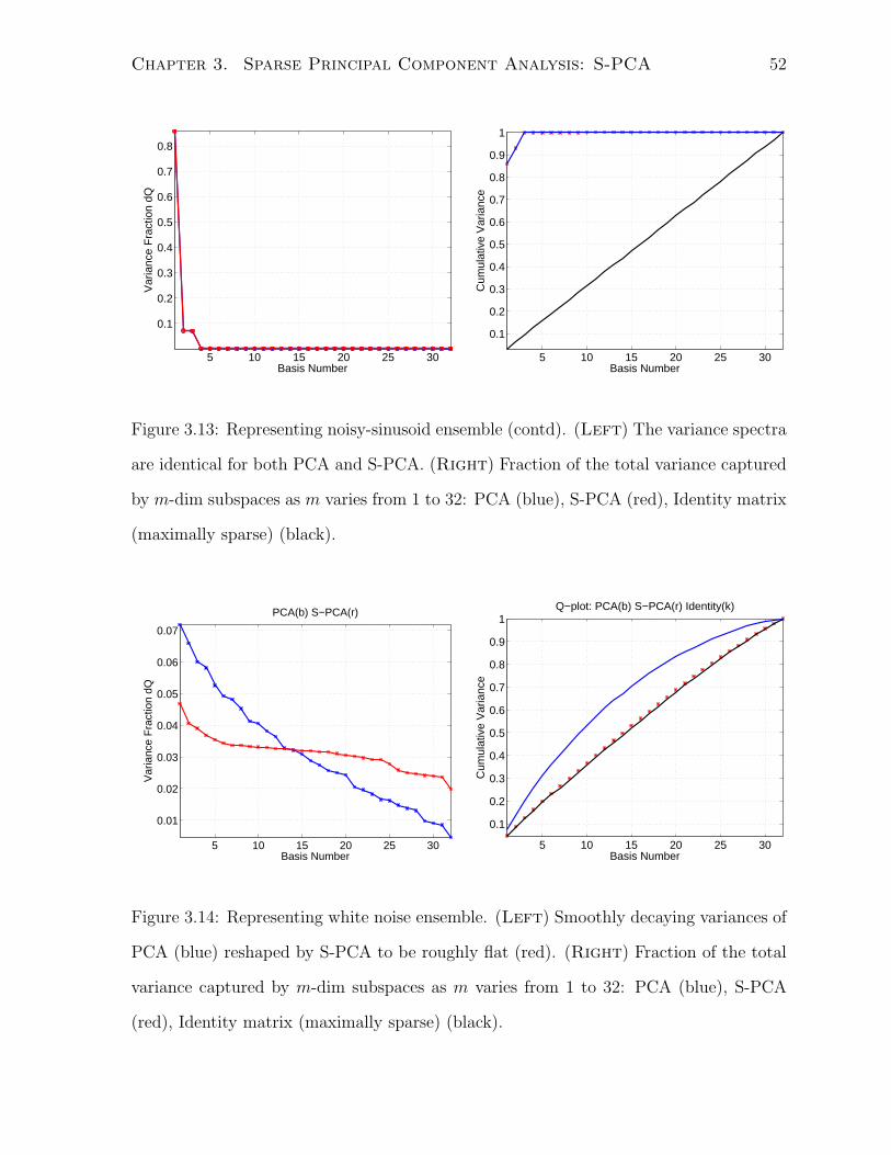
Chapter 3. Sparse Principal Component Analysis: S-PCA 52
5 10 15 20 25 30
0.1
0.2
0.3
0.4
0.5
0.6
0.7
0.8
Basis Number
Var
ianc
e F
ract
ion
dQ
5 10 15 20 25 30
0.1
0.2
0.3
0.4
0.5
0.6
0.7
0.8
0.9
1
Basis Number
Cum
ulat
ive
Var
ianc
e
Figure 3.13: Representing noisy-sinusoid ensemble (contd). (Left) The variance spectra
are identical for both PCA and S-PCA. (Right) Fraction of the total variance captured
by m-dim subspaces as m varies from 1 to 32: PCA (blue), S-PCA (red), Identity matrix
(maximally sparse) (black).
5 10 15 20 25 30
0.01
0.02
0.03
0.04
0.05
0.06
0.07
Basis Number
Var
ianc
e F
ract
ion
dQ
PCA(b) S−PCA(r)
5 10 15 20 25 30
0.1
0.2
0.3
0.4
0.5
0.6
0.7
0.8
0.9
1Q−plot: PCA(b) S−PCA(r) Identity(k)
Basis Number
Cum
ulat
ive
Var
ianc
e
Figure 3.14: Representing white noise ensemble. (Left) Smoothly decaying variances of
PCA (blue) reshaped by S-PCA to be roughly flat (red). (Right) Fraction of the total
variance captured by m-dim subspaces as m varies from 1 to 32: PCA (blue), S-PCA
(red), Identity matrix (maximally sparse) (black).

Chapter 3. Sparse Principal Component Analysis: S-PCA 53
PCA
S-PCA
Figure 3.15: Representing white noise ensemble (contd). (Top) PCA and (Bottom)
S-PCA. Each waveform is 32 pixels long. In each waveform the zero line is near the
median value of the waveform.

Chapter 3. Sparse Principal Component Analysis: S-PCA 54
3.5.1 Facelets
We represent face images that have been acquired under roughly similar viewing condi-
tions with a varying degree of pose change [80]. For such an image collection we argue
that the ensemble can be decomposed using a multi-scale, local basis. Each basis vec-
tor represents a spatially coherent image blob. The spatial coherence is caused by the
consistency in the overall shape of the object and in the shape of its parts across the
ensemble.
The PCA representation displayed in Fig. 2.8 is typical of the results obtained for
object specific image ensembles. In particular, the first few principal vectors are relatively
smooth and represent global correlations. As the index m increases (i.e. the variance of
the component decreases), the basis vectors represent finer spatial structure but remain
global in space. This is apparent in Fig. 2.8 from the relative sizes of the individual
regions in which the basis functions are of one sign, which get increasingly smaller with
increasing index. Unfortunately, it is impossible to tell from the PCA basis whether or
not such fine scale structure is correlated across the entire image.
The first few basis vectors for the S-PCA results on the face ensemble represent
correlations across the whole image (see Fig. 3.16). However, as the index increases, the
basis vectors become quite sparse, indicating that the information at finer spatial scales
is not strongly correlated across the entire image.
3.5.2 Handlets
In Fig. 3.17 we show results from applying S-PCA on the hand image ensemble. The first
few basis vectors represent correlations across the whole image. In particular, for pixels
in large coherent regions, such as the back of the hand, the extent of the correlation is
large. However, as the basis index increases, the basis vectors become quite sparse by
being dominant only in local regions. This indicates that the information at finer spatial

Chapter 3. Sparse Principal Component Analysis: S-PCA 55
Figure 3.16: Sparse-PCA results on the face images. Each basis image is of size: 112×92
pixels. Subimages are rescaled to have zero value correspond to a gray level of 127.
Only the first 64 basis vectors are displayed here. Unlike PCA, here the basis vectors
representing fine-scale information are spatially localized. Compare this with the result
from PCA shown in Fig. 2.8.
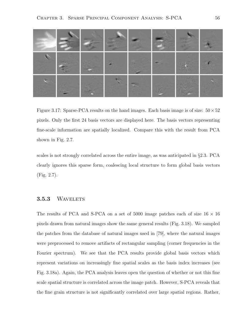
Chapter 3. Sparse Principal Component Analysis: S-PCA 56
Figure 3.17: Sparse-PCA results on the hand images. Each basis image is of size: 50×52
pixels. Only the first 24 basis vectors are displayed here. The basis vectors representing
fine-scale information are spatially localized. Compare this with the result from PCA
shown in Fig. 2.7.
scales is not strongly correlated across the entire image, as was anticipated in §2.3. PCA
clearly ignores this sparse form, coalescing local structure to form global basis vectors
(Fig. 2.7).
3.5.3 Wavelets
The results of PCA and S-PCA on a set of 5000 image patches each of size 16 × 16
pixels drawn from natural images show the same general results (Fig. 3.18). We sampled
the patches from the database of natural images used in [79], where the natural images
were preprocessed to remove artifacts of rectangular sampling (corner frequencies in the
Fourier spectrum). We see that the PCA results provide global basis vectors which
represent variations on increasingly fine spatial scales as the basis index increases (see
Fig. 3.18a). Again, the PCA analysis leaves open the question of whether or not this fine
scale spatial structure is correlated across the image patch. However, S-PCA reveals that
the fine grain structure is not significantly correlated over large spatial regions. Rather,
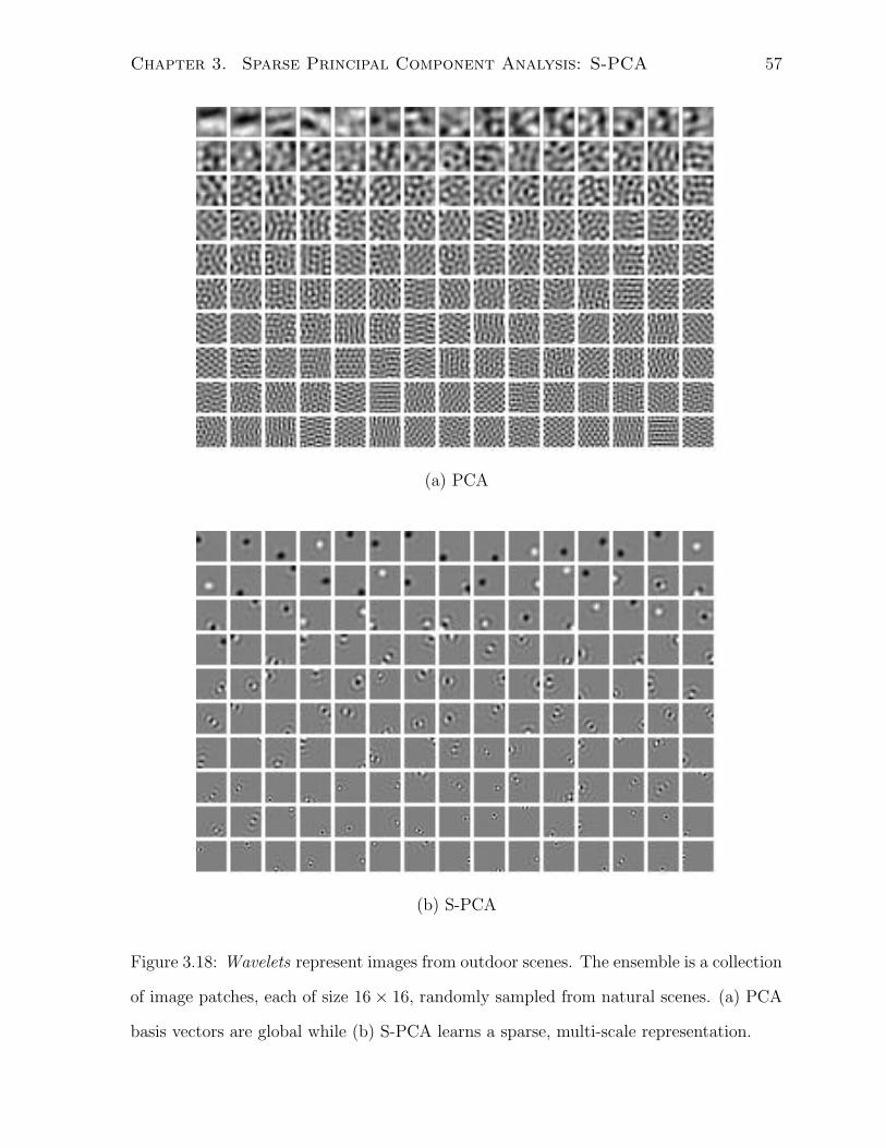
Chapter 3. Sparse Principal Component Analysis: S-PCA 57
(a) PCA
(b) S-PCA
Figure 3.18: Wavelets represent images from outdoor scenes. The ensemble is a collection
of image patches, each of size 16× 16, randomly sampled from natural scenes. (a) PCA
basis vectors are global while (b) S-PCA learns a sparse, multi-scale representation.

Chapter 3. Sparse Principal Component Analysis: S-PCA 58
Figure 3.19: PCA results on the optical flow fields measured from an image sequence of
a bush moving in the wind. The flow fields are sampled in 16× 16 pixel blocks.
as the basis index increases, the S-PCA basis vectors exhibit increasingly local structure
(Fig. 3.18b). Here the fine scale basis vectors appear to have either a center-surround
structure or are similar to orientation tuned, scale-specific filter kernels.
3.5.4 Flowlets
The results from training PCA and S-PCA on a set of 5000 flow fields obtained from
an outdoor motion sequence are presented in Figs. 3.19 and 3.20. The flow fields are
sampled in 16 × 16 pixel blocks1. We see that the PCA results provide global vector
1We thank Michael Black for the motion sequence and the optical flow fields (http://www.cs.brown.edu/~black/images.html).

Chapter 3. Sparse Principal Component Analysis: S-PCA 59
Figure 3.20: Flowlets represent optical flow fields measured from an image sequence of a
bush moving in the wind. The flow fields are sampled in 16× 16 pixel blocks.

Chapter 3. Sparse Principal Component Analysis: S-PCA 60
fields which vary on increasingly fine scales as the basis index increases (Fig. 3.19). The
PCA analysis leaves open the question of whether or not the fine scale structure of the
flow is correlated across the image patch. However, S-PCA reveals multi-scale structure
in a way similar to the ensembles considered so far.
3.6 Enforcing Sparsity by Coring
In deriving the S-PCA basis, we encourage sparsity, which means the basis elements may
be close to zero but need not be exactly zero. If the basis elements were to be exactly
zero, then we can avoid doing extra arithmetic operations. How might we achieve this?
One idea is to apply a “sharper” prior while learning the S-PCA basis, that is to use a
probability model with a large mass at the origin. In the extreme case, the prior could
take the shape of a mixture model, e.g. a impulse function with unit area at the origin
suitably mixed with a large-scale Gaussian. The problem with such a prior is that the
impulse function makes the optimization difficult.
Adopting a mixture model form for the sparse prior is a good idea, and we discuss this
later in the thesis. Here we overcome the problem of basis elements not being exactly zero
by simply coring them, i.e., basis elements that are “small” are reset to zero. However,
there is a problem: coring destroys the orthogonality property of the S-PCA basis. The
non-orthogonality is annoying because the basis coefficients can no longer be obtained
by simple projections and the energy along one basis direction depends on all the others.
For an optimal coefficient set, we need to use the (pseudo–) inverse of the non-orthogonal
basis. Moreover, this pseudo-inverse is unlikely to be a sparse matrix, i.e. the zeroes we
introduce in coring are filled again with non-zero values in the corresponding elements of
the pseudo-matrix. Obviously, we would like to avoid computing the inverse and we show
how to do this next. For demonstration we pick the task of reconstructing an image.

Chapter 3. Sparse Principal Component Analysis: S-PCA 61
3.6.1 Iterative Image Reconstruction
Consider the following linear model for an image ~x
~x = B~c,
where the coefficient vector ~c is obtained by projecting the image onto the orthonormal
S-PCA basis B,
~c = BT~x.
Let B represent the cored S-PCA basis,
B = bBc, (3.8)
where for a given threshold ε, the basis elements in B = bi,j are cored to B = bi,j
based on their sizes “relative” to the maximum absolute value in B:
bi,j =
bi,j if|bi,j |
maxk,l|bk,l|> ε,
0 otherwise.
(3.9)
Once the bases are cored, there is no reason for B to be orthogonal. Hence, a simple
projection of ~x onto the basis B would be insufficient to produce the exact coefficients ~c
that can represent ~x. The optimal coefficient vector using the cored basis,
~c = arg min~c
∥∥∥ ~x− B~c∥∥∥
2(3.10)
requires a pseudo-inverse
~c =(BT B
)−1
BT~x. (3.11)
Note the matrix-vector operations: B~c and BT~x, are sparse but the pseudo-inverse(BT B
)−1
is unlikely to be sparse and hence we wish to avoid this computation. So
consider the following iterative procedure to build the coefficients:
~c0 = ~0,
~cn+1 = ~cn + BT (~x− B~cn). (3.12)
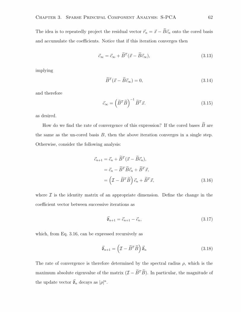
Chapter 3. Sparse Principal Component Analysis: S-PCA 62
The idea is to repeatedly project the residual vector ~rn = ~x − B~cn onto the cored basis
and accumulate the coefficients. Notice that if this iteration converges then
~c∞ = ~c∞ + BT (~x− B~c∞), (3.13)
implying
BT (~x− B~c∞) = 0, (3.14)
and therefore
~c∞ =(BT B
)−1
BT~x. (3.15)
as desired.
How do we find the rate of convergence of this expression? If the cored bases B are
the same as the un-cored basis B, then the above iteration converges in a single step.
Otherwise, consider the following analysis:
~cn+1 = ~cn + BT (~x− B~cn),
= ~cn − BT B~cn + BT~x,
=(I − BT B
)~cn + BT~x, (3.16)
where I is the identity matrix of an appropriate dimension. Define the change in the
coefficient vector between successive iterations as
~dn+1 = ~cn+1 − ~cn, (3.17)
which, from Eq. 3.16, can be expressed recursively as
~dn+1 =(I − BT B
)~dn (3.18)
The rate of convergence is therefore determined by the spectral radius ρ, which is the
maximum absolute eigenvalue of the matrix (I − BT B). In particular, the magnitude of
the update vector ~dn decays as |ρ|n.

Chapter 3. Sparse Principal Component Analysis: S-PCA 63
There are two user-defined thresholds implicit in the iterative process. The first one
is the constant ε used in Eq. 3.9 to enforce sparsity on the S-PCA basis vectors. We
chose a value of ε = 0.05, which means all the S-PCA basis elements that are below 5%
of the maximum absolute value in the basis matrix get suppressed to zero. We need an
additional constant to help terminate the iterative process. For this we compare in each
iteration the magnitude of the error vector ~δcn with the norm of the coefficient
‖~dn‖1 < ν‖~cn‖1.
We set the tolerance parameter ν to a value 10−2. We apply this analysis for reconstruct-
ing images in a database of eye images, which we discuss next.
3.6.2 Eyelets
We train S-PCA on a database of eye images. The training images have been cropped
from the FERET database [87]. The original face images were scaled and rotated so that,
in the warped image, the left and right eyes have a horizontal separation of 40 pixels.
These warped images were then cropped to 20 × 25 regions around each eye, resulting
in a database of 2392 eye images (Fig. 4.1). Furthermore, these images were contrast-
normalized to minimize the effects of shading and specularity. We defer the actual details
of this normalization to the next chapter.
The PCA and the S-PCA basis, called Eyelets, are shown in Figs. 3.21 and 3.22,
respectively. We use both PCA and S-PCA representations to do the reconstruction. For
a given subspace dimensionality, on the training set PCA has to do better than S-PCA
in minimizing the reconstruction error. However, with sparsity enforced via coring and
the iterative procedure just outlined for computing a coefficient vector, the S-PCA basis
vectors must be computationally more efficient for reconstruction.
In Fig. 3.22 we see that as the basis index increases the S-PCA bases appear increas-
ingly sparse. In fact, coring basis elements which are less than 5% of the maximum

Chapter 3. Sparse Principal Component Analysis: S-PCA 64
Figure 3.21: The leading 200 PCA bases for eye images, displayed in the decreasing
order of the input variance they capture, beginning at the top left corner and going
horizontally across the page. Observe the fine-scale information, captured by the high-
order eigenvectors, is spread across the entire image.
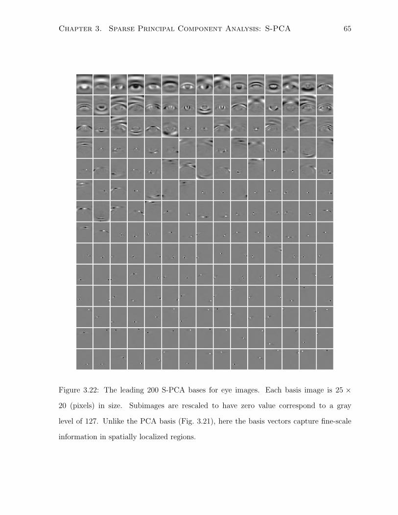
Chapter 3. Sparse Principal Component Analysis: S-PCA 65
Figure 3.22: The leading 200 S-PCA bases for eye images. Each basis image is 25 ×
20 (pixels) in size. Subimages are rescaled to have zero value correspond to a gray
level of 127. Unlike the PCA basis (Fig. 3.21), here the basis vectors capture fine-scale
information in spatially localized regions.

Chapter 3. Sparse Principal Component Analysis: S-PCA 66
20 40 60 80 100
0.1
0.2
0.3
0.4
0.5
0.6
0.7
Number of Basis
Sparsity−Fraction (b), |ρ| (r)
20 40 60 80 100
2
2.5
3
3.5
4
Number of Basis
Average Iterations
Figure 3.23: (Left) Sparsity Fraction (blue) and the magnitude of the leading eigenvalue
λ (red). (Right) Average Number of Iterations taken to compute the coefficient vector.
absolute value, causes the S-PCA matrix, constructed from the leading 100 basis vectors,
to be over 70% sparse. In Fig. 3.23 we measure this sparsity fraction, which is the ratio
of the number of zeros in the matrix to the total size of the matrix, as a function of the
subspace dimensionality.
Coring however causes the S-PCA basis to be non-orthogonal. A measure of this
non-orthogonality is given by the magnitude of the leading eigenvalue |ρ| for the matrix:(I − BT B
). If the cored basis are orthogonal, then we expect ρ to be zero. From
Fig. 3.23 we observe that there is a steady increase in ρ as a function of the subspace
dimensionality.
As we noted earlier, the rate of convergence of the iterative process, for computing
coefficients of the cored basis, is proportional to |ρ|n – the higher the magnitude of ρ, the
slower is the decay rate. From Fig. 3.23, we can see that the average number of iterations
it takes to converge is small even for a 100 dimensional subspace.
We also measure the relative error between the norm of the reconstruction error
and the norm of the input image, as a function of the subspace dimensionality. From
Fig. 3.24 we can see that PCA and S-PCA offer similar relative error values when the

Chapter 3. Sparse Principal Component Analysis: S-PCA 67
20 40 60 80 100
0.3
0.35
0.4
0.45
0.5
0.55
0.6
Number of Basis
Rel
ativ
e E
rror
PCA (b) S−PCA (r)
20 40 60 80 1000.2
0.4
0.6
0.8
1
1.2
1.4
1.6
1.8
2x 10
5
Number of Basis
Flo
p C
ount
PCA (b) S−PCA (r)
Figure 3.24: (Left) Reconstruction Error from PCA (blue) S-PCA (red). (Right)
Average Flop Count with PCA (blue) and S-PCA (red).
subspace dimensionality is small. However, with increasing index PCA gives a much
better performance. Also in Fig. 3.24 we plot the average number of flops used for
reconstruction from the cored S-PCA basis and compare it with the PCA basis. The
flop count by S-PCA basis for a 50-dimensional subspace indicates it is about 40% faster
than the PCA basis. To achieve even better performance, we would need to decrease
the spectral radius of(I − BT B
), perhaps by encouraging the S-PCA coefficients to
be closer to zero while still maintaining orthogonality so that coring is less severe. We
return to this issue later in the thesis.
Finally, we show how distorted the reconstructions can be from the cored basis. We
discuss a perceptual distortion measure in the following chapter, but here we perform a
simple visual comparison of the reconstruction results from PCA, cored S-PCA and the
pseudo-inverse computation (Eq. 3.11). Given the cored basis, the result from pseudo-
inverse computation is the optimal. In Fig. 3.25 we show reconstruction results for a
sample of random images in the eye database. The top row contains the input images
and within each sub-figure, the top row is the result from S-PCA basis, the middle row
from the pseudo-inverse computation and the last row is the PCA result. The results

Chapter 3. Sparse Principal Component Analysis: S-PCA 68
validate the iterative reconstruction approach we have taken with the cored S-PCA basis.
However, as we mentioned earlier, we can improve the flop count with S-PCA basis by
driving hard on sparsity, while learning the basis directions.
3.7 Related Work
The relationship to sparse coding and ICA has already been discussed in the previous
chapter. With sparse coding (or ICA) the optimization process can be expensive, so it is
often the case that basis functions are learned on sub-images (say 16×16 image patches)
extracted from a larger image. As a consequence, spatial structure larger than an image
block may never be captured. In this context, it is worth mentioning that the image size
is much less of a restriction for S-PCA. For example, the images in the face database have
a size of 112× 92 pixels and the database has 400 images. S-PCA has been successful in
highlighting the multi-scale structure in this ensemble.
Varimax is one of the earliest known references for rotating principal components so
that the basis vectors are more interpretive [50]. The rotation is performed to increase the
variance of the elements that describe the basis vectors. In our framework this increase
in variance will also increase the cost term C2. As we have shown, for basis directions to
provide a meaningful representation for naturally-occurring ensembles, we found it useful
to draw the basis elements from a low-entropy distribution.
The idea of applying a sparse constraint on the weights of a neural net appears
in [78, 122]. The networks are non-linear and the learning has not shown the ability
to extract multi-scale structure. Recently, such sparsity constraints were extended to
both the basis matrix and the coefficients as in [48] but this algorithm is likely to have
problems with the size of the input image. Our learning algorithm has a flavor similar
to the one used in [20] where the tensor properties of the cumulants for the coefficient
densities are exploited using a rotation based Jacobi algorithm. For the application of

Chapter 3. Sparse Principal Component Analysis: S-PCA 69
(a) Eye Images
(b) Reconstruction with 10-dimensional subspace.
(c) Reconstruction with 20-dimensional subspace.
(d) Reconstruction with 50-dimensional subspace.
(e) Reconstruction with 100-dimensional subspace.
Figure 3.25: Reconstruction of input eye images in (a) as a function of the subspace
dimensionality. With in each subfigure the results are: (Top) iterative reconstruction
from cored S-PCA, (Middle) pseudo-inverse with cored S-PCA and (Bottom) PCA.

Chapter 3. Sparse Principal Component Analysis: S-PCA 70
sparsity in regression and kernel analysis see [76,106,108].
The notion of sparsity also appears in the basis selection literature. The idea is to have
a dictionary of basis functions, possibly multi-scale, and pick a small number of them to
represent the input image [22]. The basis functions are either predefined, as in wavelets,
or specific to a class, as in correlation-based kernels [81,85]. Unfortunately, determining
coefficients for each image is formulated as a quadratic programming problem and this
can be computationally very expensive. In [44,59,91] a constraint of positiveness on the
basis elements, called non-negative matrix factorization (NMF), appears to lead to facial
features at a single scale. Finally, a Bayesian treatment of Sparse-PCA is given in [116],
which postdates our original publication of S-PCA [24].

Chapter 4
Contrast-Invariant
Appearance-Based Detection
4.1 Introduction
In this chapter we propose two different models for contrast-invariant appearance de-
tection. The contrast signal, which is the intensity variation around a mean brightness
value, can be measured in two ways, either by an object-specific, global model or a
generic, local method. Once the dataset is adjusted for contrast, a representation is
built using the principal subspace (within-space) and its orthogonal complement (out-of-
subspace). We experiment with principal subspaces obtained by PCA and S-PCA basis
vectors. An important feature of our system is a perceptual distortion measure that we
designed to compare the appearance of an object to its reconstruction from the principal
subspace. By distortion we mean the reconstruction error caused by not including the
out-of-subspace signal. We show how to use S-PCA basis trained on generic background
patches to decide if two images are perceptually similar.
Our work builds upon four key observations on subspace-based representations. First,
subspace methods involve least squares approximations which are notoriously sensitive
71

Chapter 4. Contrast-Invariant Appearance-Based Detection 72
to large outliers. Hence, it is important to account for outliers in training, and testing,
subspace methods [17, 30]. A related issue is one of variation in the image contrast. In
general, images with higher contrasts have larger variance. If some images have variance
much larger than others then these images can potentially skew the estimation of the
object-specific subspace. Often a contrast normalization step is performed, either by
histogram equalization or by normalizing the variance (or the power) of an image so that
it is of unit length. We offer two alternative normalization strategies which we feel are
more appropriate for object-specific ensembles.
Second, S-PCA amounts to a rotation of input coordinate axes and, as such, it does
not define a probability density model for the input data. However, subspaces can also
be derived from the perspective of density estimation [75, 92, 109]. The advantage in
estimating the input density is that it allows for the design of probabilistic methods
to detect, recognize and/or classify test images as appearances of known objects. In
particular, one strategy for object representation is to divide the signal space into a
principal subspace and its orthogonal complement and then build probability models
separately for the two subspaces. Then the detection strategy is to apply a threshold on
the likelihood assigned by the combined density model to a test image [75].
The third key observation, as noted in [25,74], is that the variance estimate per–pixel
given by the subspace density models for the residual signal in the out–of–subspace is
overly conservative [75, 109]. We defer the actual details of variance estimation used in
our appearance-based detector to a later section.
Finally, the detection problem can be posed as one of assessing image similarity, where
the issue is to develop a measure that captures the notion that two images are perceptu-
ally similar. It is well known that standard error norms, such as the mean-squared-error
(MSE), are unsuitable for measuring perceptual distortion. Recent successes in formulat-
ing perceptual distortion norms (e.g., [105]) have come from analyzing the psychophysics
of spatial pattern detection, particularly contrast and orientation masking, and under-

Chapter 4. Contrast-Invariant Appearance-Based Detection 73
standing the functional properties of neurons in the primary visual cortex. A typical
perceptual distortion model consists of a linear transformation of images by a “hand-
crafted” wavelet representation that is tuned to different spatial orientations and scales,
followed by a divisive normalization mechanism. The normalization scheme involves pool-
ing information in adjacent wavelet channels (that is in neighbouring spatial locations,
orientations and scales, eg. [18]). Normalization provides a context for local significance,
in that a high sensor channel (wavelet) response is down-weighted if the adjacent channels
are equally active but upgraded otherwise. The full set of normalized sensors tuned for
different spatial positions, spatial frequencies, orientations and contrast discrimination
bands provide a basis for assessing the perceptual similarity between two images. Our
work generalizes this normalization scheme to object-specific multi-scale representations
derived from S-PCA.
While we concentrate on sub-space methods, much work has also been done in building
feature-based object detectors [98, 104], in particular systems where the features are
simple to compute and hence the objects are fast to detect [3, 39,82,117].
4.2 Datasets
We investigate two different image datasets: eyes/non-eyes [25] and faces/non-faces [6].
The eye images are regions cropped from the FERET face database [87]. The face images
were first scaled and rotated such that, in the warped image, the centers of left and right
eyes have a horizontal separation of 40 pixels. From these warped images, we crop image
regions around the eyes, each of size 20 × 25 pixels, to generate a database of 2392 eye
patches (Fig. 4.1).
For non-eyes, we construct a generic background patch ensemble by running an inter-
est point detector [97] on several different natural images and collecting image patches
with detector responses above a certain threshold (Fig. 4.2). The interest point detector
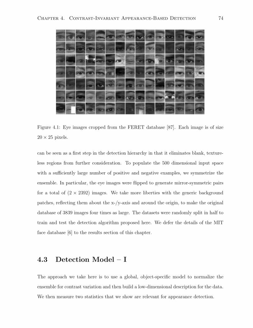
Chapter 4. Contrast-Invariant Appearance-Based Detection 74
Figure 4.1: Eye images cropped from the FERET database [87]. Each image is of size
20× 25 pixels.
can be seen as a first step in the detection hierarchy in that it eliminates blank, texture-
less regions from further consideration. To populate the 500 dimensional input space
with a sufficiently large number of positive and negative examples, we symmetrize the
ensemble. In particular, the eye images were flipped to generate mirror-symmetric pairs
for a total of (2 × 2392) images. We take more liberties with the generic background
patches, reflecting them about the x-/y-axis and around the origin, to make the original
database of 3839 images four times as large. The datasets were randomly split in half to
train and test the detection algorithm proposed here. We defer the details of the MIT
face database [6] to the results section of this chapter.
4.3 Detection Model – I
The approach we take here is to use a global, object-specific model to normalize the
ensemble for contrast variation and then build a low-dimensional description for the data.
We then measure two statistics that we show are relevant for appearance detection.

Chapter 4. Contrast-Invariant Appearance-Based Detection 75
Figure 4.2: Generic background patches detected by an interest point detector [97]. The
image size is 20× 25.
4.3.1 Contrast Model for an Object-Specific Ensemble
Contrast is defined as the variation in image intensities around a mean brightness value.
We can extend this contrast model to be global and explicit for an object-specific ensemble
by using two basis vectors, namely a constant “DC” basis vector and a vector in the
direction of the mean of the training set after removing the contribution from the DC
basis. We define the training set as~tkK
k=1where K is the total number of training
images and ~tk is the kth training image stored in a column format. Each element of the
DC vector ~ξ is given by
ξi = 1/√
N, (4.1)
where N is the total number of pixels in the image, and ~ξ is of unit length. The mean
image ~µ is derived from the training set after removing the DC contribution, that is
~µ ∝ 1
K
K∑
k=1
[~tk − ~ξ
(~ξ T~tk
)], (4.2)

Chapter 4. Contrast-Invariant Appearance-Based Detection 76
and ~µ is normalized to be of unit length. We define the components of ~tk in the directions
of the DC and the mean vector as
dk = ~ξ T~tk (4.3)
and
mk = ~µ T~tk (4.4)
respectively.
The goal here is to generate a subspace representation for the spatial structure of
the eye images that is insensitive to contrast changes. We wish to capture the spatial
structure by a basis matrix B given by
B =
[~b1
~b2 · · · ~bN
]. (4.5)
It is possible that the spatial structure of eye images, and thus the basis matrix B,
changes as the mean component mk increases. Alternatively, these basis images may
stay roughly the same and only the variation of their coefficients increases with the mean
component mk. The coefficient ck,j in the direction of jth basis vector for the kth image
is given by,
ck,j = ~b Tj~tk. (4.6)
Indeed, if the variation of the mean component is primarily due to lighting and imaging
effects, then we might assume that the underlying signal, i.e. the spatial structure of eye
images, is invariant to contrast. In this case we would expect the basis images ~bj to be
independent of mk and only the variance of coefficients ck,j to scale as a function of mk.
We test this hypothesis by analyzing the relationship between the mean component
mk and the contrast variance lk, given by
lk =1
N
∥∥∥~tk − dk~ξ −mk~µ
∥∥∥2
2, (4.7)
where ‖·‖22 is the expression for the square of the two-norm and lk determines the variance-
per-pixel that remains unaccounted for, after using the DC and the mean vectors to de-
scribe the ensemble. In Fig. 4.3(Left) we plot the contrast variation√
lk as a function

Chapter 4. Contrast-Invariant Appearance-Based Detection 77
of the mean coefficient mk for each eye image. Notice that there are a large range of
variances in the training images, with those images with larger values of the mean coef-
ficient having significantly larger variances. As a rough approximation this relationship
can be modeled by a straight line fit to the data, shown by the black line going through
the origin in Fig. 4.3(Left). Note, the straight line fit is biased by the constraint that
it passes through the origin (denoting perfect contrast invariance). From Fig. 4.3(Left)
there appears to be a trend away from the line for smaller values of the mean coefficient.
We suspect this is due to the use of a single mean image, which may not model the lower
contrast images particularly well.
To balance the variances across different image contrasts, we rescale the training
images to get
~qk =
[~tk − dk
~ξ −mk~µ]
s(mk), (4.8)
where s(mk) is a scaling factor for training image ~tk with mean coefficient mk. It is
convenient to assume a minimum value for the left-over variance, say due to independent
pixel noise, and use this in the estimate for scaling:
s(mk) =√
σ2min + f(mk). (4.9)
The red curve in Fig. 4.3(Left) is a plot of s(mk) with f(mk) = p × m2k, where p is
the slope of the straight line fit (the black line in Fig. 4.3(Left)), and σmin = 8. After
normalization, all the scaled images falling on the red curve shown in Fig. 4.3(Right)
will have a left-over-variance value of one. We discuss next how to use the rescaled images
for training a principal subspace.
4.3.2 Principal Subspace and its Complement
Once the images are rescaled into ~qk for k = 1, · · · , K, we first trim the database by
removing extreme images that either have a low or negative mean image coefficient (≤ 20)
and/or very large left-over variances per pixel (> 25). Most of these extreme images have

Chapter 4. Contrast-Invariant Appearance-Based Detection 78
−500 0 500 10000
50
100
150
200
Std
. Dev
./pix
el
Mean Coeff
Contrast Dependent Image Variation
−1000 −500 0 500 10000
5
10
15
20
25
Mean Coeff
Std
. Dev
. (pe
r pi
xel)
Rescaled Image Std.Dev.
Figure 4.3: Contrast dependency of the Eye Dataset.
identifiable problems, such as the eye being closed, not centered, having a different scale,
or having reflections from glasses. For the database we consider here they constitute only
a small fraction of the input data: 46 out of 2392 eye images in the training set. We
then use singular value decomposition (SVD) to perform principal component analysis.
The PCA bases are shown in Fig. 4.4. The PCA basis in turn are used as a starting
point for training the S-PCA representation. The S-PCA basis is trained for a complete
representation of the input space, that is, the basis matrix is square. The resulting S-PCA
basis are shown in Fig. 4.5.
Let ~bj denote the basis images obtained either by PCA or S-PCA and σ2j the variance
obtained by projecting the data onto the basis direction ~bj. Suppose we approximate
the normalized images ~qk with just the M leading basis images. We can compute the
residual signal ~ek in the complement space as
~ek = ~qk −M∑
j=1
ck,j~bj, (4.10)
where the expansion coefficient is given by
ck,j = ~b Tj ~qk, (4.11)
and M is taken to be much less than the total number of training images K and the total

Chapter 4. Contrast-Invariant Appearance-Based Detection 79
Figure 4.4: PCA basis for the eye space, arranged from left to right in decreasing order
of the input variance captured. The first sub-image on the left is the mean image.

Chapter 4. Contrast-Invariant Appearance-Based Detection 80
Figure 4.5: S-PCA basis for the eye space, arranged from left to right in decreasing order
of the input variance captured. The first sub-image on the left is the mean image.
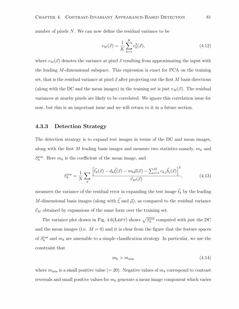
Chapter 4. Contrast-Invariant Appearance-Based Detection 81
number of pixels N . We can now define the residual variance to be
vM(~x) =1
K
K∑
k=1
e2k(~x), (4.12)
where vM(~x) denotes the variance at pixel ~x resulting from approximating the input with
the leading M -dimensional subspace. This expression is exact for PCA on the training
set, that is the residual variance at pixel ~x after projecting out the first M basis directions
(along with the DC and the mean images) in the training set is just vM(~x). The residual
variances at nearby pixels are likely to be correlated. We ignore this correlation issue for
now, but this is an important issue and we will return to it in a future section.
4.3.3 Detection Strategy
The detection strategy is to expand test images in terms of the DC and mean images,
along with the first M leading basis images and measure two statistics namely, mk and
Soosk . Here mk is the coefficient of the mean image, and
Soosk =
1
N
∑
~x
[~tk(~x)− dk
~ξ(~x)−mk~µ(~x)−∑Mj=1 ck,j
~bj(~x)]2
~vM(~x), (4.13)
measures the variance of the residual error in expanding the test image ~tk by the leading
M -dimensional basis images (along with ~ξ and ~µ), as compared to the residual variance
~vM obtained by expansions of the same form over the training set.
The variance plot drawn in Fig. 4.6(Left) shows√
Soosk computed with just the DC
and the mean images (i.e. M = 0) and it is clear from the figure that the feature spaces
of Soosk and mk are amenable to a simple classification strategy. In particular, we use the
constraint that
mk > mmin (4.14)
where mmin is a small positive value (= 20). Negative values of mk correspond to contrast
reversals and small positive values for mk generate a mean image component which varies

Chapter 4. Contrast-Invariant Appearance-Based Detection 82
only by a few gray levels. Additionally, we apply a simple contrast invariant threshold
of the form
arctan(mk,√
Soosk ) ≤ τoos, (4.15)
which requires that the distribution of the eye dataset be underneath a line drawn through
the origin at an angle τoos for successful detection. A particular detector is then defined
by the number of basis vectors used for the principal subspace and the choice of the
parameter τoos.
4.3.4 Results
We first discuss results from using the PCA basis and then show the improvement in
performance obtained by the S-PCA basis. While the eye data is split into training
and testing sets, the generic background patch ensemble is considered as one large test
dataset.
In Figs. 4.6 and 4.7 we show the separation of the test datasets: eyes (green) and
non-eyes (red), in the feature space of√
Soosk vs mk, as a function of the increasing
subspace dimensionality (M = 0, 20, 50, and 100). The detection threshold lines drawn
as black lines in each one of the plots generate roughly 5% false positives. The true
detection/rejection rates and the corresponding ROC curve obtained by changing the
value of the τoos parameter can be seen in more detail in Fig. 4.8. The simplest strategy
of using just the DC and the mean images (i.e. M = 0) results in a detection rate of
93% and a false target rate of 7%. With increasing subspace dimensionality, the datasets
appear to be more separable visually, however the improvement in the ROC curves is
marginal. In particular, a 50-dimensional PCA subspace is suitable for describing the
eye manifold, as the true detection rate grows to 95% and the false positive rate reduces
to ≈ 5.5% and increasing M further causes over-fitting on the training set, as seen from
the ROC plots in Fig. 4.9.
The discriminative ability of the PCA representation is not high. Is there any im-
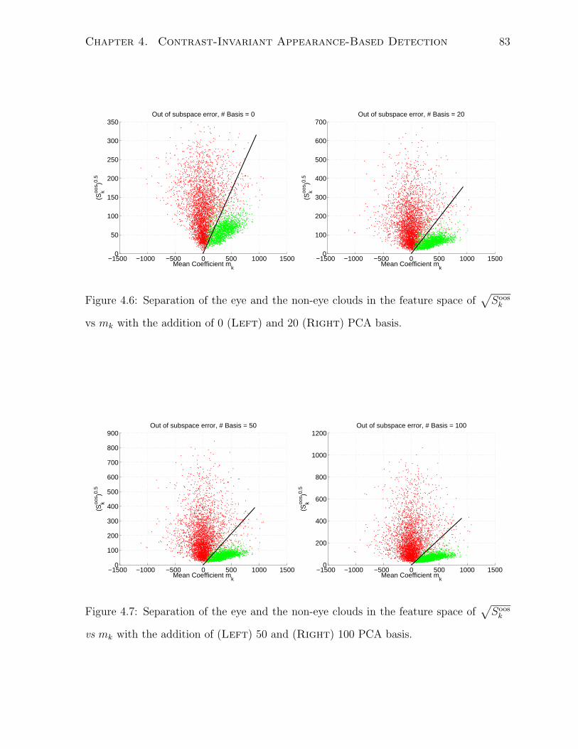
Chapter 4. Contrast-Invariant Appearance-Based Detection 83
−1500 −1000 −500 0 500 1000 15000
50
100
150
200
250
300
350Out of subspace error, # Basis = 0
Mean Coefficient mk
(Soo
sk
)0.5
−1500 −1000 −500 0 500 1000 15000
100
200
300
400
500
600
700Out of subspace error, # Basis = 20
Mean Coefficient mk
(Soo
sk
)0.5
Figure 4.6: Separation of the eye and the non-eye clouds in the feature space of√
Soosk
vs mk with the addition of 0 (Left) and 20 (Right) PCA basis.
−1500 −1000 −500 0 500 1000 15000
100
200
300
400
500
600
700
800
900Out of subspace error, # Basis = 50
Mean Coefficient mk
(Soo
sk
)0.5
−1500 −1000 −500 0 500 1000 15000
200
400
600
800
1000
1200Out of subspace error, # Basis = 100
Mean Coefficient mk
(Soo
sk
)0.5
Figure 4.7: Separation of the eye and the non-eye clouds in the feature space of√
Soosk
vs mk with the addition of (Left) 50 and (Right) 100 PCA basis.
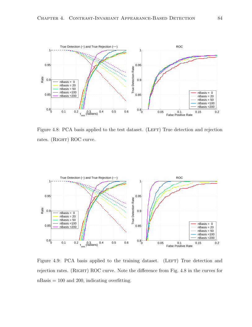
Chapter 4. Contrast-Invariant Appearance-Based Detection 84
0 0.1 0.2 0.3 0.4 0.5 0.60.8
0.85
0.9
0.95
1True Detection (−) and True Rejection (−−)
τoos
(radians)
Rat
e
nBasis = 0nBasis = 20nBasis = 50nBasis =100nBasis =200
0 0.05 0.1 0.15 0.20.8
0.85
0.9
0.95
1ROC
False Positive Rate
Tru
e D
etec
tion
Rat
e
nBasis = 0nBasis = 20nBasis = 50nBasis =100nBasis =200
Figure 4.8: PCA basis applied to the test dataset. (Left) True detection and rejection
rates. (Right) ROC curve.
0 0.1 0.2 0.3 0.4 0.5 0.60.8
0.85
0.9
0.95
1True Detection (−) and True Rejection (−−)
τoos
(radians)
Rat
e
nBasis = 0nBasis = 20nBasis = 50nBasis =100nBasis =200
0 0.05 0.1 0.15 0.20.8
0.85
0.9
0.95
1ROC
False Positive Rate
Tru
e D
etec
tion
Rat
e
nBasis = 0nBasis = 20nBasis = 50nBasis =100nBasis =200
Figure 4.9: PCA basis applied to the training dataset. (Left) True detection and
rejection rates. (Right) ROC curve. Note the difference from Fig. 4.8 in the curves for
nBasis = 100 and 200, indicating overfitting.

Chapter 4. Contrast-Invariant Appearance-Based Detection 85
0 0.1 0.2 0.3 0.4 0.5 0.60.8
0.85
0.9
0.95
1True Detection (−) and True Rejection (−−)
τoos
(radians)
Rat
e
nBasis = 0nBasis = 20nBasis = 50nBasis =100nBasis =200
0 0.05 0.1 0.15 0.20.8
0.85
0.9
0.95
1ROC
False Positive Rate
Tru
e D
etec
tion
Rat
e
nBasis = 0nBasis = 20nBasis = 50nBasis =100nBasis =200
Figure 4.10: S-PCA basis applied to the test dataset. (Left) True detection and rejection
rates. (Right) ROC curve.
0 0.1 0.2 0.3 0.4 0.5 0.60.8
0.85
0.9
0.95
1True Detection (−) and True Rejection (−−)
τoos
(radians)
Rat
e
nBasis = 0nBasis = 20nBasis = 50nBasis =100nBasis =200
0 0.05 0.1 0.15 0.20.8
0.85
0.9
0.95
1ROC
False Positive Rate
Tru
e D
etec
tion
Rat
e
nBasis = 0nBasis = 20nBasis = 50nBasis =100nBasis =200
Figure 4.11: S-PCA basis applied to the training dataset. (Left) True detection and
rejection rates. (Right) ROC curve.

Chapter 4. Contrast-Invariant Appearance-Based Detection 86
provement in using the S-PCA basis? The results from applying the S-PCA basis on the
test datasets is shown in Fig. 4.10. Compared with the results obtained from using the
PCA basis, as shown in Fig. 4.8, the improvement with S-PCA basis is at most a few
percentage points. It is not surprising that PCA and S-PCA do about the same because
the reconstruction errors are roughly the same. While there is an advantage in using
S-PCA basis, in that they facilitate fast detection (see § 3.6), the recognition rates for
both PCA and S-PCA are less than satisfactory.
A closer inspection of the eyes rejected as false negatives shows that these are images
that look extreme, in that many have highlights caused by the specularities from the eye
glasses or pixel outliers such as the hair falling over the eye brows etc. It is possible to
improve on the false negative rates by taking into account only relevant portions of an
image in detecting eyes, as we have done in [25]. However, the high false positives rates
are a major cause for concern and we present a vastly improved detection model next.
4.4 Detection Model – II
The problem of detecting known appearances is analogous to the problem of measuring
image similarity, in that we need a perceptual error norm for meaningful results. In
§ 4.3 we used a mean-squared-error (MSE) norm for measuring image distortions and we
ignored the fact that the residual errors in the out-of-subspace signal may be correlated
spatially. Thus, the detector model we proposed earlier is unlikely to capture perceptual
distances between image pairs.
Motivated by the work in [105], we propose a new detector model outlined in Fig. 4.12.
For this new detector model, we find it convenient to employ a generic, local contrast-
normalization scheme, so that there is no bias introduced by the object-specific mean
image into the dataset (Eq. 4.2). There are five steps involved: (1) contrast-normalize
(WCN ) the test image ~y to obtain ~t; (2) project ~t onto the wavelet-like space W derived

Chapter 4. Contrast-Invariant Appearance-Based Detection 87
~tWCN←−−− ~xyW T
~dBT
−−−→ ~bB−−−→ ~
dyPDN PDN
y~z ~z
Figure 4.12: Detector Model – II with perceptual distance normalization (PDN ). See
§ 4.4 for more details.
from training S-PCA on generic background patches and obtain ~d as the coefficient vector;
(3) build a low-dimensional approximation~d to the coefficient vector ~d using S-PCA
basis B constructed for the object-specific ensemble in the “wavelet” space; (4) apply
perceptual distance normalization PDN on the coefficient vector ~d and its reconstruction
~d to obtain normalized vectors ~z and ~z; and finally (5) apply a simple detection strategy
to ~z and ~z. We explain these details next.
4.4.1 Weber-Contrast Normalization
Weber-contrast is a measure of the relationship between the response of a pixel and that
of its neighborhood. In particular, if xi is the response of a pixel at location i and µi
is an estimate of the mean response value in its neighborhood, then the Weber contrast
signal ci is defined as:
ci =xi − µi
µi
. (4.17)
The mean signal value µi can be obtained by convolving the image with a two-dimensional
radially-symmetric Gaussian filter G(i ; σ). The neighborhood size is determined by the
standard deviation σ of the Gaussian function. While this contrast computation removes
shading variations, there are pixel outliers, such as the specularities from the eye glasses
or the hair falling over the eye brows, that can bias the computation (Fig. 4.1). To reduce

Chapter 4. Contrast-Invariant Appearance-Based Detection 88
Figure 4.13: Weber-contrast normalized eye dataset. Compare this with Fig. 4.1.
the effect of outliers we normalize the contrast values using the following expression:
ti = F(ci ; β),
=1− exp(−βci)
1 + exp(−βci), (4.18)
where β is chosen such that for a predefined contrast value ci = cdef, the normalized
contrast ti takes a value of 0.5.
The contrast normalization results on a subset of the eye and the non-eye datasets
are shown in Figs. 4.13 and 4.14 respectively. We set σ = 3 for estimating the contrast
and cdef = 0.3 for normalization. In Fig. 4.15 we show histograms of the pixel intensities
for the two datasets before and after normalization. The normalization removes the DC
signal for generic background patches. But for the eye ensemble, we see a small non-
zero average, caused by pixel intensities being brighter than their neighbors more often
than not. The range of intensities after normalization is compressed, that is the tails
of the distributions are clipped. In general, we observe larger values of σ improve the
performance of the detector, but the detector is less susceptible to the actual setting of
cdef.
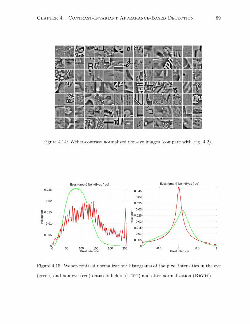
Chapter 4. Contrast-Invariant Appearance-Based Detection 89
Figure 4.14: Weber-contrast normalized non-eye images (compare with Fig. 4.2).
0 50 100 150 200 2500
0.005
0.01
0.015
0.02
0.025
Pixel Intensity
His
togr
am
Eyes (green) Non−Eyes (red)
−0.5 0 0.5 10
0.005
0.01
0.015
0.02
0.025
0.03
0.035
0.04
0.045
Pixel Intensity
His
togr
am
Eyes (green) Non−Eyes (red)
Figure 4.15: Weber-contrast normalization: histograms of the pixel intensities in the eye
(green) and non-eye (red) datasets before (Left) and after normalization (Right).

Chapter 4. Contrast-Invariant Appearance-Based Detection 90
4.4.2 S-PCA Representation: W, B
The S-PCA basis matrix trained on generic background patches is given by W , an N×N
matrix, shown in Fig. 4.16. For an N -dimensional contrast-normalized image ~t the N -
dimensional S-PCA coefficient vector is given by
~d = W T~t.
Because the S-PCA basis look like wavelets, we abuse the notation slightly to call ~d a
wavelet coefficient vector. Next, S-PCA is trained separately on the wavelet coefficients
generated for the images in the object-specific ensemble (eg. eyes). For the following
step, we build a low-dimensional representation for the wavelet coefficient vector using
the leading M object-specific S-PCA basis vectors. In particular let B be the object-
specific S-PCA basis matrix of size N × M , then projecting the wavelet coefficient ~d
gives
~b = BT ~d
and the wavelet coefficient vector can be reconstructed as
~d = B~b
= BBT ~d,
which is again N -dimensional. Because the basis matrix B resides in the wavelet space,
it is hard to interpret it and hence in Fig. 4.17 we show the matrix: W ×B obtained by
pre-multiplying object-specific S-PCA basis B by the generic background patch S-PCA
basis W . Notice, the basis W ×B is sparse, spatially local and multi-scale.
4.4.3 Perceptual Distance Normalization
The coefficient vectors ~d and~d are now subjected to a perceptual distance normalization
process. The idea is to normalize each wavelet coefficient by the pooled amplitude of
wavelet coefficients tuned to similar spatial frequencies and similar spatial neighborhoods
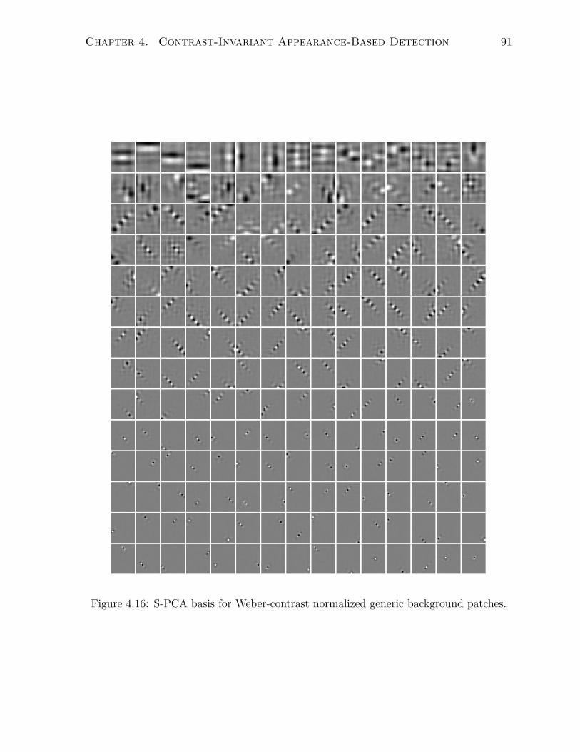
Chapter 4. Contrast-Invariant Appearance-Based Detection 91
Figure 4.16: S-PCA basis for Weber-contrast normalized generic background patches.

Chapter 4. Contrast-Invariant Appearance-Based Detection 92
Figure 4.17: S-PCA basis for Weber-contrast normalized eye images.

Chapter 4. Contrast-Invariant Appearance-Based Detection 93
0 100 200 300 400 5000
0.2
0.4
0.6
0.8
1
1.2
1.4Band Ids
Basis Channel
Sta
ndar
d D
evia
tion
Figure 4.18: (Left) Partitioning the variance spectrum into five different subsets (shown
here in different colors) each tuned to roughly similar spatial frequencies. (Right) An
eye image and its bandpass components from the five different basis bands (Top), the
corresponding amplitude maps (Middle) and the corresponding Fourier magnitude maps
for the bandpass images (Bottom).
[18, 105]. Because S-PCA basis are learned from the data, as opposed to being hand-
crafted, we need to find what the adjacent scales and orientations are for each S-PCA
basis function in an automatic fashion. We outline a simple strategy next.
The spatial frequency tuning of the wavelets in W was observed to be related to
the variance of the wavelet coefficients over the training set. Therefore by partitioning
the variance spectrum we obtain subsets of wavelets tuned to roughly similar spatial
frequencies. We automated this partitioning using K-means on the log variance spectrum.
The result is shown in Fig. 4.18(Left), where the spectrum is partitioned into 5 groups,
each drawn in a different color for the generic background patch ensemble.
To identify the local amplitude of image structure in each frequency band we form
the amplitude image using a band of S-PCA basis indexed from l to h,
~p =
∣∣∣∣∣∑
l≤k≤h
~wkdk
∣∣∣∣∣ . (4.21)
Here ~wk denotes the kth basis vector, dk is the corresponding wavelet coefficient value. In

Chapter 4. Contrast-Invariant Appearance-Based Detection 94
Fig. 4.18(Right, Top) we show an eye image and the bandpass images that result from
the summation in Eq. 4.21 in each of the five different basis bands. In Fig. 4.18(Right,
Middle) we show the eye image along with its amplitude maps that result from the ab-
solute operation over the bandpass images shown before, as given in Eq. 4.21. To provide
a better intuition for the bandpass images, the images in Fig. 4.18(Right, Bottom)
show the Fourier magnitudes of the bandpass images. To estimate the portion of this
amplitude image within the spatial support of the kth wavelet ~wk, we compute:
sk =∣∣~wT
k
∣∣ ~p. (4.22)
It can be shown that sk ≥ |dk| with the equality holding when dj = 0 for j 6= k.
We can finally express the perceptual distance normalization (PDN ) of the kth ele-
ment of the coefficient vector as
zk =dk
(sk + υlh). (4.23)
The constant υlh is a saturation parameter for the basis band indexed from l to h.
It is determined empirically by processing random images with a predetermined noise
level (= 4 gray levels) and measuring the statistics of the resulting S-PCA coefficients.
In particular, the random images are contrast normalized and for each wavelet band
a corresponding amplitude map is generated. The amplitude maps are then projected
back into the wavelet space and the saturation constant υlh is set to the median value
of the coefficients of the amplitude map in each wavelet band. The perceptual distance
normalized coefficients of a wavelet coefficient vector ~d and its reconstruction~d are given
by vectors ~z and ~z respectively.
4.4.4 Detection Strategy
For the purpose of detection we measure two numbers: (1) the wavelet norm given by
the L1 norm of ~z; and (2) the error norm given by the L1 norm of the error vector ~z− ~z.

Chapter 4. Contrast-Invariant Appearance-Based Detection 95
We study the variation of these two numbers as a function of the increasing subspace
dimensionality M , the number of columns in the basis matrix B shown in Fig. 4.13 (for
relevant discussion see §4.4.2). We expect the error norm to be high for generic image
patches because the subspace was built for the object-specific ensemble. Also, we expect
that the higher the wavelet norm, the higher will be the error norm for generic image
patches. In fact, as we discuss next, what we observe is that the generic background
patches and the object-specific ensemble appear as two distinguishable clouds with a
small amount of overlap. We next present results using a straightforward detection
strategy.
4.4.5 Results
Eyes/Non-Eyes:
In Figs. 4.19 and 4.20, we show the results of applying the new detection method on the
test set of eyes/non-eyes by varying M = 20, 50, 100, 200. For clarity the plots have
been scaled in such a way as to show all of the eye images (green points) at the expense of
omitting a portion of the non-eye images (red points). As a detection strategy, we adopted
a very simple approach of using a line aligned with the principal axis of the generic image
patch cloud as shown in Fig. 4.21(Left) for the test set and Fig. 4.22(Left) for the
training set. Points below the line are taken as positive detections. The ROC curve for a
given M is obtained by adjusting the y-intercept of the line and these are shown for both
the test and train sets. For example, in Fig. 4.21(Left) the two black lines correspond
to two different points on the ROC curve (M = 50) shown in Fig. 4.21(Right).
The ROC curve in Fig. 4.21(Right) for the test set makes one thing very clear: the
false positives can be kept very low, namely a value less than 0.8%, for a true acceptance
rate of ≈ 95% in a M = 50 dimensional subspace. This is a significant improvement over
the previously reported detection model results (see Figs. 4.8 and 4.10). For comparison,

Chapter 4. Contrast-Invariant Appearance-Based Detection 96
60 70 80 90 100 110 120 13050
60
70
80
90
100
110
120
130
140
Wavelet Norm
Err
or N
orm
#Basis: 20
60 70 80 90 100 110 120 130
50
60
70
80
90
100
110
120
130
140
Wavelet Norm
Err
or N
orm
#Basis: 50
Figure 4.19: Separation of the eye and the non-eye clouds in the test set with the addition
of (Left) 20 and (Right) 50 SPCA basis.
the ROC curve with M = 50 from Fig. 4.8 is reproduced here as a black line. In
particular, for M = 50 the gain in false positive rate with PDN is nine-fold for a true
detection rate of 95% and is 24-times better for a true detection rate of 90%. Some of
the false positives admitted by the detection algorithm are shown in Fig. 4.23. The false
positives were collected over the training and testing datasets and displayed in a single
figure for convenience.
Faces/Non-Faces:
The MIT face database [6] consists of 2429/472 training/testing face images and 4548/23573
training/testing non-face images. Informally, most of the images in the training set are:
cropped above the eyebrows, cropped just below the bottom lip, centered, roughly frontal
views, and relatively well exposed. However, very few of the images in the test set appear
to satisfy all these properties. We therefore created “mixed” training and testing sets
by merging all these face images, adding the mirror symmetric versions, then randomly
selecting half the dataset for mixed-training and the other half for mixed-testing. In
Fig. 4.24(Left) we plot the perceptually normalized space for the newly created mixed-

Chapter 4. Contrast-Invariant Appearance-Based Detection 97
60 70 80 90 100 110 120 130
40
60
80
100
120
140
Wavelet Norm
Err
or N
orm
#Basis: 100
60 70 80 90 100 110 120 130
30
40
50
60
70
80
90
100
110
120
Wavelet Norm
Err
or N
orm
#Basis: 200
Figure 4.20: Separation of the eye and the non-eye clouds in the test set with the addition
of (Left) 100 and (Right) 200 SPCA basis.
60 70 80 90 100 110 120 130
50
60
70
80
90
100
110
120
130
140
Wavelet Norm
Err
or N
orm
#Basis: 50
0 0.01 0.02 0.03 0.04 0.05 0.06 0.07 0.08 0.09 0.10.8
0.85
0.9
0.95
1ROC
False Positive Rate
Tru
e D
etec
tion
Rat
e
M = 20M = 50M = 100M = 200M = 50 [I]
Figure 4.21: Detection results on the test set. (Left) Strategy is to adjust the y-intercept
of a line aligned with the principal axis of the non-eye cloud (red). Points below the line
are taken as positive detections. The two black lines correspond to two different points
on the ROC curve for M = 50 (green) shown on the (Right). For comparison, the
ROC curve for detector model I with M = 50 (from Fig. 4.8) is reproduced here on the
(Right) as a black line (labeled M = 50 (I)).

Chapter 4. Contrast-Invariant Appearance-Based Detection 98
60 70 80 90 100 110 120 130
40
60
80
100
120
140
Wavelet Norm
Err
or N
orm
#Basis: 50
0 0.01 0.02 0.03 0.04 0.05 0.06 0.07 0.08 0.09 0.10.8
0.85
0.9
0.95
1ROC
False Positive Rate
Tru
e D
etec
tion
Rat
e
nBasis = 20nBasis = 50nBasis = 100nBasis = 200
Figure 4.22: Detection results on the training set. (Left) Strategy is to adjust the
y-intercept of a line aligned with the principal axis of the non-eye cloud (red). Points
below the line are taken as positive detections. The two black lines correspond to two
different points on the ROC curve for M = 50 shown in the (Right).
testing set, where the non-faces are indicated by red dots and the faces by the blue and
green dots. In particular, the green dots indicate faces from the original training set and
blue dots indicate faces from the original testing set. Using a subspace of M = 50 dimen-
sions, for a false positive rate of 0.1% we observe 16% false negatives, out of which 96%
belong to the original testing set. In fact, the face images in the original testing set make
up 16% of the mixed dataset and, given the separation between the original training and
original testing face images in the perceptually normalized space, this is not a surprise.
In Fig. 4.24(Right) the black curve denotes the recognition rates obtained using just
the original training set, and omitting the original test set, in a M = 50 dimensional
subspace. The recognition rates are near perfect.
Comparison with Support Vector Machine (SVM)
We compare the performance of our detector with a support vector machine (SVM)
classifier [115]. SVM is parameterized by a kernel function and a C value which is the cost

Chapter 4. Contrast-Invariant Appearance-Based Detection 99
(a) False positives
(b) Reconstruction from a 50 dimensional subspace
Figure 4.23: (Top) False positives collected over the training and testing sets and dis-
played in one figure. (Top) Reconstruction results from a 50 dimensional subspace.

Chapter 4. Contrast-Invariant Appearance-Based Detection 100
40 60 80 10020
30
40
50
60
70
80
90
100
Wavelet Norm
Err
or N
orm
M = 50
0 0.01 0.02 0.03 0.04 0.05 0.06 0.07 0.08 0.09 0.10.8
0.85
0.9
0.95
1ROC
False Positive Rate
Tru
e D
etec
tion
Rat
e
M = 20M = 50M = 100M = 200M = 50(T)
Figure 4.24: Detection results on the MIT face database. (Left) Characterizing test-
faces (blue), train-faces (green) (which together constitute the mixed-test set) and non-
faces in the test set (red) in the perceptually normalized space. (Right) ROC curves for
the “mixed” test set. The black curve denotes recognition rate for just the train-faces in
the “mixed” test set.
per unit violation of the classifier margin. We used a publicly available implementation
of SVM [6]. We chose a Gaussian kernel and varied the σ parameter. The C value was
set to 1, other values were tried but did not have a significant effect on the classifier.
On the eye dataset for different values of σ we observed a large variation in the to-
tal number of support vectors returned. In particular, for σ = [3, 5, 10, 20] the number
of support vectors returned on the training set are [5267, 1564, 1140, 1616] respectively.
Each support vector involves a dot product and hence, for a fair comparison the number
of support vectors returned should be comparable to the number of inner products per-
formed with the PDN model for a suitable choice of M . Thus, we selected σ = [5, 10]
and M = [50, 100].
In Fig. 4.25(Left) we compare the detection results from SVM to our PDN model
on the eye dataset. The green and the blue curves denote the use of M = [50, 100]
dimensional subspaces with the PDN model. The PDN graphs are identical to the
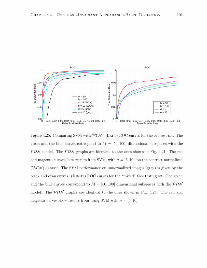
Chapter 4. Contrast-Invariant Appearance-Based Detection 101
0 0.01 0.02 0.03 0.04 0.05 0.06 0.07 0.08 0.09 0.10.8
0.85
0.9
0.95
1ROC
False Positive Rate
Tru
e D
etec
tion
Rat
e
M = 50M = 100σ = 5 (WCN)σ = 10 (WCN)σ = 5 (gray)σ = 10 (gray)
0 0.01 0.02 0.03 0.04 0.05 0.06 0.07 0.08 0.09 0.10.8
0.85
0.9
0.95
1ROC
False Positive Rate
Tru
e D
etec
tion
Rat
e
M = 50M = 100σ = 5σ = 10
Figure 4.25: Comparing SVM with PDN . (Left) ROC curves for the eye test set. The
green and the blue curves correspond to M = [50, 100] dimensional subspaces with the
PDN model. The PDN graphs are identical to the ones shown in Fig. 4.21. The red
and magenta curves show results from SVM, with σ = [5, 10], on the contrast normalized
(WCN ) dataset. The SVM performance on unnormalized images (gray) is given by the
black and cyan curves. (Right) ROC curves for the “mixed” face testing set. The green
and the blue curves correspond to M = [50, 100] dimensional subspaces with the PDN
model. The PDN graphs are identical to the ones shown in Fig. 4.24. The red and
magenta curves show results from using SVM with σ = [5, 10].
Chapter 4. Contrast-Invariant Appearance-Based Detection 102
ones shown in Fig. 4.21. The red and magenta curves show results from using SVM
with σ = [5, 10]. The performance of SVM with σ = 10 is similar to using PDN with
M = 50. Increasing the total number of support vectors, i.e. reducing σ from 10 to 5,
improves the performance of SVM. In addition, we tested the performance of the SVM
on the original gray-level images (i.e. without WCN ), and the results are given by the
black and cyan curves in Fig. 4.25(Left). It is clear that contrast normalization causes
a significant improvement in the performance of SVM.
We ran a similar experiment on the mixed training and testing sets that we created for
the MIT face database. The number of support vectors obtained on the mixed training
set for σ = [5, 10] are [1549, 1434] respectively. In Fig. 4.25(Right) we compare the
detection results from SVM to our PDN model on the mixed testing set. The green
and the blue curves denote the use of M = [50, 100] dimensional subspaces with the
PDN model. The PDN graphs are identical to the ones shown in Fig. 4.24. The red
and magenta curves show results from using SVM with σ = [5, 10]. The performance of
SVM with σ = 10 is similar to using PDN with M = 50. The best detection result we
obtained was for σ = 5, which required 1549 support vectors.
A detailed comparison of the different methods is beyond the scope of this thesis, for
several reasons: (1) The PDN normalization is not optimal in terms of computational
efficiency. It was designed for simplicity. The normalization of each wavelet should
depend only on a few “neighbouring” wavelets, and there is likely to be a more efficient
way to do this than by generating the amplitude map; (2) It is not clear that the SVM
implementation we have used is optimal (e.g. see [107]). If neither method is optimal,
a detailed comparison may not be very revealing. Perhaps, most interesting is the use
of several detectors (e.g. an eye, a nose, a mouth, and a face detector) within a single
system. For such a system the wavelet transform used in our approach is common to
all detectors, and hence the cost of the wavelet transform, in terms of the underlying
hardware, can be amortized.

Chapter 4. Contrast-Invariant Appearance-Based Detection 103
4.5 Conclusion
Using PCA models, in place of S-PCA, we have observed detection results similar to
the ones shown in Fig. 4.21 for both the object-specific and background ensembles with
the same PDN formulation as provided in Eq. 4.21–4.23. The improved performance
with PDN comes with a price, in that the images have to be represented in the full
N -dimensional wavelet domain. However, we expect wavelet decomposition of signals to
be a standard pre-processing tool. The simplicity of the detector in the wavelet domain
is striking. In particular, after applying a linear model of eyes and doing perceptual
normalization we can simply use the L1 norm to separate classes.

Chapter 5
S-PCA: Conclusions and Future
Work
We presented a novel framework, Sparse Principal Component Analysis (S-PCA), for
extracting multi-scale structure from data. We showed how introducing a sparsity con-
straint on the elements of a basis matrix recovers structure in spatially coherent image
blobs and provides a multi-scale representation for the ensemble. The principal advan-
tages of S-PCA over a standard PCA based representation include an intuitive under-
standing of the features underlying the ensemble and efficiency in computations resulting
from a sparse basis representation.
Sparsity in the basis matrix is best understood as saving computations over the life-
time of a representation system. However, in encoding images there are a few extra
bits spent because S-PCA coefficients are correlated slightly. The learning algorithm of
S-PCA is very simple, consisting of successive planar rotations of pairs of basis vectors.
We have demonstrated the suitability of this algorithm for large-dimensional spaces.
The formulation of S-PCA is novel in that multi-scale representations emerge for a
wide variety of ensembles using just the second-order correlations. We believe the feasi-
bility of extracting multi-scale structure from second-order statistics is a point overlooked
104
Chapter 5. S-PCA: Conclusions and Future Work 105
in the literature.
We briefly outline two proposals for future work. First, in learning the basis directions
the S-PCA formulation presented here does not take into account the presence of noise in
the dataset. For a recent attempt in this direction see [116]. In the next section (§ 5.1.1),
we sketch a well-known information-theory based algorithm called Infomax [63] that
takes into account the effect of noise in the input and show how to modify it to provide a
sparse representation. Second, in deriving the S-PCA basis we encourage sparsity, which
means a majority of the basis elements may be close to zero, but they need not be exactly
zero. If the basis element values were indeed zero, then we can save lots of arithmetic
operations. So we briefly consider the possibility of driving sparsity harder by using a
mixture-of-Gaussian prior in § 5.1.2.
5.1 Future Work
5.1.1 Sparse-Infomax
Linsker’s Infomax principle states that a network is optimal if the mutual information
between its input and output is maximal [63]. The network is considered noisy. In
particular, the input to the network ~t comes from an unknown source signal ~s that has
been corrupted by (photon) noise ~p, as in
~t = ~s + ~p.
We will assume that the source vectors have an unknown covariance C given by
E(~s~s T
)= C,
where E is the expectation operator, and the noise vectors are uncorrelated in directions
each with a σ2p variance,
E(~p~p T
)= σ2
pI,

Chapter 5. S-PCA: Conclusions and Future Work 106
where I is an identity matrix of appropriate dimension. Combining these two equations
gives the covariance Q for the observables ~t
E(~t~t T)
= C + σ2pI
= Q
The network is assumed to be linear, where the input image ~t is represented by a coeffi-
cient vector ~c given by simple projection onto the basis direction matrix W
~c = W T~t.
It is easy to show that
E(~c~c T
)= W T QW.
Also, there is quantization noise at the output which is modelled as uncorrelated additive
noise ~q with variance
E(~q~q T
)= σ2
qI,
and hence the output ~z is given by
~z = ~c + ~q.
The covariance of the output signal can be expressed as
E(~z~z T
)= W T QW + σ2
qI
The InfoMax criterion is to find a basis matrix W that maximizes the mutual informa-
tion between the unknown source input and the quantized output given by:
MI(~s ; ~z) = log∣∣W T QW + σ2
qI∣∣− log
∣∣σ2pW
T W + σ2qI∣∣ .
If σ2p is zero, then there is an analytical solution to the basis matrix, which is given by
W = R× F,

Chapter 5. S-PCA: Conclusions and Future Work 107
where R is a matrix of eigenvectors for the covariance matrix C and F is a diagonal
matrix inversely proportional to the square root of the eigenvalues of C. Hence, F acts
as a whitening filter in the limit of zero noise in the input. But if the input noise is non
zero, then F sets elements on the diagonal to zero in directions where the signal power
is less than the power of noise [8, 63].
We can modify the InfoMax framework to accommodate a sparsity term on the basis
elements and we call this procedure Sparse-Infomax. In particular, we can continue to
assume a simplified form for the basis matrix W = R× F as given above, but introduce
a sparse prior on the elements of the R matrix.
The objective function in Sparse-InfoMax will be set up to maximize the mutual
information between the input and the output of the network, while promoting sparsity
via a regularization term on the basis elements. Additionally, a pre-specified bit budget
can be imposed on the outputs, just as in the Infomax framework. For sparsity, the
following functional form can be applied on the basis elements rij:
∑
ij
log p(rij) ∝∑
ij
log
(α + β × exp
(−∣∣∣∣rij
γ
∣∣∣∣))
,
where α, β and γ are the parameters of the sparsity driving function. The constraint of
bit budget K can be incorporated into the cost function in the following way:
∑
i
(log[E(z2
i )]− log σ2
q
)−K = 0,
where E(z2i ) is the variance in each output channel.
5.1.2 Encouraging Sparsity with a Mixture-of-Gaussian Prior
We briefly consider a Gaussian mixture model to drive sparsity in the basis directions.
In particular, elements of a basis vector ~bk are driven by a two-component Gaussian
mixture,
p(bik) = mnkN (bik ; σ2n) + (1−mnk)N (bik ; σ2
bk),

Chapter 5. S-PCA: Conclusions and Future Work 108
where bik is the ith element of the kth basis vector ~bk, p(bik) is the prior probability
distribution on the basis elements and N (· ; ·) represents a Gaussian distribution. There
are two Gaussian distributions here, one that is narrow with variance σ2n and the other
component is broad with variance σ2bk.
The narrow Gaussian has a mixing coefficient mnk, which is also a function of the
basis vector index k. This dependency is natural as we expect the mixing coefficient for
coarse-scale S-PCA basis functions to be close to zero, but a lot higher for the fine-scale
basis vectors. In comparison, for the PCA basis or a pixel basis (identity matrix) we
expect mnk to be independent of the basis index k. For example, we expect the higher-
order PCA basis to have mnk = 0 and the identity matrix (or the pixel basis) to have
mnk = N−1N
, accounting for the fact that there is only one pixel on in each basis vector.
The mixture model has several independent parameters but there is a constraint
binding them all, as we show next. The S-PCA representation is orthonormal and hence
the basis vectors have unit length,
∑
i
b2ik = 1.
The variance computation on the basis elements leads to
1
N
∑
i
b2ik =
1
N,
and this in turn gives rise to a linear constraint on the variance of the mixture model:
mnkσ2n + (1−mnk)σ
2bk =
1
N,
where N is the length of the basis vector ~bk. Given mnk this is a linear equation in the
parameters σ2n and σ2
bk, so there is a one-parameter family of solutions for each mixing
coefficient mnk. The goal here is to drive sparsity hard. We achieve this by annealing
the parameter σ2n that is independent of the basis index k.
In each sweep of the S-PCA rotations, we hold the mixture model parameters constant
for each basis vector, and update the basis directions. Then, in iteration t+1, the variance

Chapter 5. S-PCA: Conclusions and Future Work 109
parameter σ2n is lowered by setting
σ2n(t + 1) = ρ× σ2
n(t).
Using the new value of σ2n(t + 1) and the old value of σ2
bk(t) we fit mnk(t + 1) for each
basis vector ~bk using a typical EM procedure. Finally, given the new value of mnk(t + 1)
and σ2n(t + 1), we can use the linear constraint mentioned above to update σ2
bk:
σ2bk =
1
(1−mnk)
(1
N−mnkσ
2n
).
For initialization of this new process, it seems convenient to use the S-PCA basis
produced by the algorithm proposed earlier in the thesis.
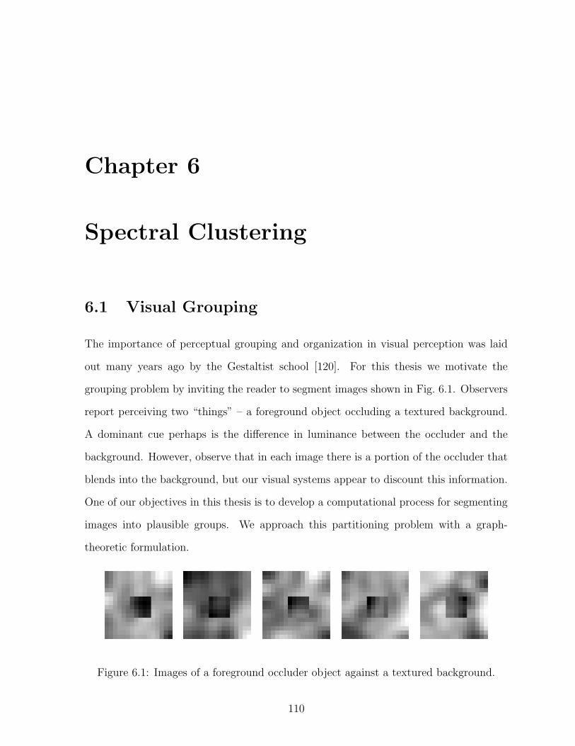
Chapter 6
Spectral Clustering
6.1 Visual Grouping
The importance of perceptual grouping and organization in visual perception was laid
out many years ago by the Gestaltist school [120]. For this thesis we motivate the
grouping problem by inviting the reader to segment images shown in Fig. 6.1. Observers
report perceiving two “things” – a foreground object occluding a textured background.
A dominant cue perhaps is the difference in luminance between the occluder and the
background. However, observe that in each image there is a portion of the occluder that
blends into the background, but our visual systems appear to discount this information.
One of our objectives in this thesis is to develop a computational process for segmenting
images into plausible groups. We approach this partitioning problem with a graph-
theoretic formulation.
Figure 6.1: Images of a foreground occluder object against a textured background.
110

Chapter 6. Spectral Clustering 111
6.2 Graph-Theoretic Partitioning
We consider partitioning a weighted undirected graph G into a set of discrete clusters.
Each node in the graph corresponds to a pixel in the image, and the edges correspond to
the strength (or affinity) with which two nodes belong to one group. Ideally, the nodes
in each cluster should be connected with high-affinity edges, while different clusters are
either disconnected or are connected only by a few edges with low affinity. The practical
problem is to identify these tightly coupled clusters, and cut the inter-cluster edges.
6.2.1 Graph Formulation
For illustration purposes we consider an ensemble of random test images formed from
two independent samples of 2D Gaussian filtered white noise (see Fig. 6.1). One sample
is used to form the 16× 16 background image, and a cropped 5× 5 fragment of a second
sample is used for the foreground region. A small constant bias is added to the foreground
region.
A graph clustering problem is formed where each pixel in the test image is associated
with a vertex in the graph G. The edges in G are defined by the standard 8-neighbourhood
of each pixel (with pixels at the edges and corners of the image only having 5 and 3
neighbours, respectively). A weight is associated with each edge based on some property
of the pixels that it connects. For example, the affinities between pixels (or nodes) ~xi
and ~xj will correspond to how much the two pixels agree in luminance, color, texture
etc. and how far apart they are in the image. The affinities are captured in a symmetric
n× n matrix A with ai,j ≥ 0 and ai,j = aj,i. For the images considered in this thesis, we
use intensities at pixels ~xi and ~xj denoted by I(~xi) and I(~xj) and define affinity as
ai,j =
exp
−[I(~xi)−I(~xj)
]2(2σ2)
for ~xj in the 8-neighbourhood of ~xi,
0 otherwise,
(6.1)

Chapter 6. Spectral Clustering 112
where σ is a grey-level standard deviation. We use
σ = ρ× g,
where g is the median absolute difference of gray levels between all neighbouring pixels
and ρ = 1.5. It is worth mentioning that for the clustering algorithms that we propose
later in this thesis, ρ can be set anywhere between 1 and 2.
We make note of one other property of the graph, which is the degree dj of a node j.
It is defined to be
dj =n∑
i=1
ai,j =n∑
i=1
aj,i, (6.2)
and consider a diagonal matrix D which is stacked with the degrees of the nodes as in
D = diag
[d1 d2 . . . dn
]. (6.3)
This generative process provides an ensemble of clustering problems that we feel are
representative of the structure of typical image segmentation problems. In particular, due
to the smooth variation in gray-levels, there is some variability in the affinities within both
foreground and background regions. Moreover, due to the use of independent samples for
the two regions, there is often a significant step in gray-level across the boundary between
the two regions. Finally, due to the small bias used, there is also a significant chance
for pixels on opposite sides of the boundary to have similar gray-levels, and thus high
affinities. This latter property ensures that there are some edges with significant weights
between the two clusters in the graph associated with the foreground and background
pixels.
The affinity matrices for images in Fig. 6.1 may be less intuitive to interpret, so we
show datasets that have a simple distribution in two-dimensional space as in Figure 6.2a.
The affinities were designed to fall off rapidly as a function of the Euclidean distance
between points. Because the dataset is well separated in space, the corresponding affinity
matrix, shown in Fig. 6.2b, has a pronounced block structure. For convenience, the

Chapter 6. Spectral Clustering 113
(a) Well separated (b) Affinities (c) Weakly separated (d) Affinities
Figure 6.2: Two sets of points in a plane and the corresponding affinity matrices. The
affinities are designed to fall off rapidly as a function of the Euclidean distance between
points.
affinity matrix has been arranged to have the points appear sorted. Specifically, the
points are sorted based on the angle made by the lines joining each of the points in
the dataset to the overall mean of the dataset. Because we know the generative model
for the dataset, we also know the overall cluster center. The angle sorting procedure
groups all the points in a cluster together and makes the block diagonal structure of
the affinity matrix obvious. For comparison, we show a weakly coupled dataset and its
affinity matrix in Fig. 6.2c and Fig. 6.2d respectively. Observe the cross-talk, or the weak
coupling, between clusters in the affinity matrix in Fig. 6.2d.
6.2.2 Cut Measures / Criterion
To partition the graph we need a cut measure and a cut criterion. For now, consider
segmenting the image (graph) into two clusters, a foreground object F and a background
object B. Define a corresponding cut measure AFB to be the sum of the affinities for all
the edges that begin in the foreground cluster and end in the background object:
AFB =∑
i∈F,j∈B
ai,j .

Chapter 6. Spectral Clustering 114
Foreground F Background B Complete Graph G
Foreground F AFF =∑
i∈F,j∈F ai,j AFB =∑
i∈F,j∈B ai,j AFG = AFF + AFB
Background B ABF =∑
i∈B,j∈F ai,j ABB =∑
i∈B,j∈B ai,j ABG = ABF + ABB
Table 6.1: A summary of cut measures. AFB and ABF summarize the connections between
the foreground and the background objects. Observe AFB has the same value as ABF
because the affinity matrix A is symmetric. AFG and ABG summarize the connections
from the foreground and the background to the complete graph.
Similarly, define ABF to be the sum of the affinities for all the edges that begin in the
background object and end in the foreground cluster:
ABF =∑
i∈B,j∈F
ai,j.
Because the affinity matrix is symmetric, AFB = ABF . In Table 6.1 we list several possible
cut measures that arise when the graph is partitioned into two groups. In particular, we
have:
AFF =∑
i∈F,j∈F
ai,j ,
ABB =∑
i∈B,j∈B
ai,j ,
AFG = AFF + AFB,
ABG = ABB + ABF .
There are many possible alternatives for a cut criterion, but here we will discuss a
recent proposal, called Normalized Cut [101]. We will also show how this criterion leads
us to a random walk perspective for graph partitioning, which we investigate in depth in
the following chapter. The goal with normalized cut (NCut) is to minimize the following
criterion:
NCut =AFB
AFG
+ABF
ABG
, (6.4)

Chapter 6. Spectral Clustering 115
Cut Criterion
Normalized Cut [101] AFB
AFG
+ ABF
ABG
Foreground Cut [86] AFB
AFF
Min-Max Cut [33] AFB
AFF
+ ABF
ABB
Conductance [51] AFB
min(
AFG,ABG
)
Table 6.2: A summary of cut criteria based on the measures given in Table 6.1.
over all possible foreground and background partitions (F,B). Minimizing NCut means
identifying two tightly coupled clusters with relatively small affinities between the two
clusters. NCut is also an attempt to remove any biases that are in favor of cutting small
isolated modes in the graph (as in [123]). In Table 6.2 we list several possible cut criteria,
where each criterion was shown to be optimal for a particular distribution of points in a
dataset [33,51,86]. Not surprisingly, optimizing the NCut criterion is NP hard [26,101].
We now turn to spectral-based methods for an approximate way of solving the NCut
criterion. We will then discuss a recent proposal for partitioning the graph into K (> 2)
clusters. Finally, we will discuss very briefly a random walk view of spectral clustering.
We will also highlight an important assumption underlying the spectral methods.
6.3 Spectral-based Methods
Spectral graph methods have gained popularity in a variety of application domains in-
cluding segmenting images [68, 96]; clustering parallel scientific computation tasks [88]
and circuit layouts [4, 21] among others. Here we explore how spectral methods provide
an approximate solution to the NCut problem.

Chapter 6. Spectral Clustering 116
6.3.1 NCut algorithm
The minimization of NCut criterion has an approximate solution and it is based on
solving a generalized eigenvalue problem [101]. The NCut algorithm uses the Laplacian
matrix
Q = D − A (6.5)
where A is the affinity matrix (Eq. 6.1) and D is the diagonal matrix of degree values
(Eq. 6.3). The algorithm consists of solving the generalized eigen problem:
Q~u = λD~u. (6.6)
The solution consists in analyzing the structure of the eigenvector associated with the
second smallest eigenvalue of (6.6). In particular, it is shown in [101] that when there is
a partitioning of the image into the foreground F and background B such that
ui =
α, i ∈ F
β, i ∈ B
(6.7)
then (F,B) is the optimal NCut and the value of the cut itself is NCut(F,B) = λ. A
vector ~u satisfying condition Eq. 6.7 is called piecewise constant with respect to the
partition (F,B). The partitioning of the second smallest eigenvector can be done by
thresholding its elements. This in turn induces a partitioning of the graph into (F,B).
To obtain K clusters where K > 2 we have to proceed recursively. It is conceivable that
using more eigenvectors and directly computing a K way partitioning is perhaps a better
option [5].
6.3.2 K–Means Spectral Clustering
While much of the earlier work in spectral graph partitioning dealt with finding just two
partitions [26], here we consider one particular proposal for finding a K-way partitioning.

Chapter 6. Spectral Clustering 117
This proposal builds on the prior work of using K eigenvectors simultaneously to perform
K-way partitioning of the data (e.g. [21, 77,99,101,119]).
1. From the affinity matrix A construct a symmetric normalized matrix
L = D−1/2AD−1/2.
2. Find a matrix U of eigenvectors: U = [~u1, ~u2, · · · , ~uK ], associated with the K
largest eigenvalues of L.
3. Form a matrix V by re-normalizing each row of U to be unit length:
vi,j =ui,j(∑
j u2i,j
)1/2.
4. Treat each row of V as a point in RK . Cluster them into K clusters via K-means
(or any algorithm that minimizes distance to K centers).
5. Assign node i to cluster k if and only if row i of the matrix V was assigned to
cluster k.
For K well separated clusters, it was shown in [77] that the rows of matrix V form
tight clusters around K well separated points that are orthogonal to each other on the
surface of a K sphere. As we discuss next, this property is related to having piecewise
constancy in the form of the leading K eigenvectors i.e., elements of the eigenvectors have
approximately the same value within each cluster.
6.3.3 Random Walks and Normalized Cuts
We can convert the affinity matrix A into a stochastic matrix M by a simple normalization
via the inverse of the degree matrix D [72]:
M = AD−1. (6.8)

Chapter 6. Spectral Clustering 118
This normalization causes the column sums of the matrix M to add up to 1. This is a
slight change from the notation used in [72], where they use a normalization of the form
D−1A, which causes the row sums of the resulting stochastic matrix to be 1. We chose
the formulation in Eq. 6.8 to suit the analysis we provide in later chapters.
From the theory of Markov random walks [52] the element Mi,j represents the prob-
ability of moving from node j to i in one step, given a particle is in node j. We will
discuss this formulation in greater depth in the next chapter but for now we establish the
connection to the spectral problem of NCut. In particular we can show that the NCut
formulation (6.6) and the matrix M share eigenvectors, and eigenvalues, that are similar.
Assuming eigenvector ~u and eigenvalue λ satisfy the generalized eigenvalue problem in
6.6, we can write
Q~u = λD~u.
Substituting from Eq. 6.5 for the Laplacian Q gives
(D − A)~u = λD~u.
Simplifying further using Eq. 6.8
(D −MD)~u = λD~u,
D~u−MD~u = λD~u,
MD~u = (1− λ)D~u.
Thus the NCut formulation (Eq.6.6) and the stochastic matrix M share an eigenvector
that has a simple relationship: ~u and D~u. Because D is a diagonal matrix, D~u is an
element-wise normalization of the vector ~u. Similarly the eigenvalues are λ and 1 − λ
respectively. The key aspect we focus on is the result, shown in [72], that the leading
K eigenvectors of the stochastic matrix M are piecewise constant. In this context, the
K-means spectral clustering can be seen as a method that can identify the appropriate

Chapter 6. Spectral Clustering 119
10 20 30 40 50 60 70
−1
−0.5
0
0.5
10 20 30 40 50 60 70
−1
−0.5
0
0.5
(a) Well separated (b) Weakly coupled
Figure 6.3: The three leading eigenvectors for (a) well separated and (b) weakly coupled
datasets shown in Fig. 6.2. Eigenvectors are drawn in colors: first (blue), second (red) and
third (black). For the well separated cluster the eigenvectors appear roughly piecewise
constant but not so when the cluster is weakly coupled.
piecewise constant regions in the leading K eigenvectors. We demonstrate this on datasets
that are well separated and also show how the assumption breaks down when the clusters
are not that well separated.
6.3.4 Assumption of piecewise constancy
For the dataset shown in Figure 6.2a we display the leading eigenvectors of the corre-
sponding stochastic matrix M (Eq. 6.8) in Fig. 6.3a. It is clear from the plot that the
eigenvectors are piecewise constant, i.e., the elements of the eigenvectors have approxi-
mately the same value within each cluster. However we can also see from Fig. 6.3b that
this assumption breaks down for weakly coupled clusters in that the eigenvectors do not
display the piecewise constant form.
What is the form of the eigenvectors for the occluder data? First, we show a well
separated cluster in Fig. 6.4 where the foreground occluder has structure clearly differ-
entiable from the background. Indeed the first and the second eigenvectors have the
piecewise constant form (Fig. 6.4b,c) and when K-means spectral algorithm is initiated
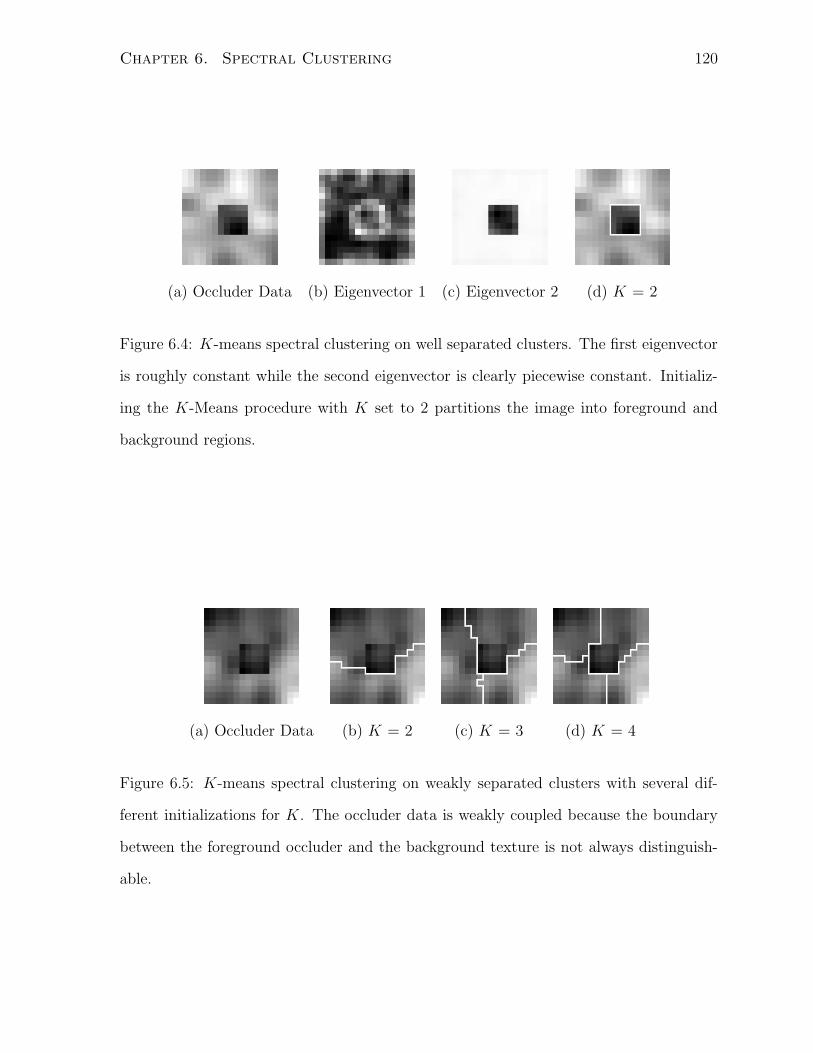
Chapter 6. Spectral Clustering 120
(a) Occluder Data (b) Eigenvector 1 (c) Eigenvector 2 (d) K = 2
Figure 6.4: K-means spectral clustering on well separated clusters. The first eigenvector
is roughly constant while the second eigenvector is clearly piecewise constant. Initializ-
ing the K-Means procedure with K set to 2 partitions the image into foreground and
background regions.
(a) Occluder Data (b) K = 2 (c) K = 3 (d) K = 4
Figure 6.5: K-means spectral clustering on weakly separated clusters with several dif-
ferent initializations for K. The occluder data is weakly coupled because the boundary
between the foreground occluder and the background texture is not always distinguish-
able.

Chapter 6. Spectral Clustering 121
Occluder Data Eigenvector 1 Eigenvector 2 Eigenvector 3 Eigenvector 4
Figure 6.6: Eigenvectors piecewise constant? Compare with Fig. 6.4b,c.
to search for 2 clusters, it finds the right partition (Fig. 6.4d).
In comparison, for a weakly coupled dataset shown in Fig. 6.5 a variety of initializa-
tions for K-means spectral clustering fail to separate the occluder from the background.
Comparing figures 6.6 and 6.4, we can see that the eigenvectors in Fig. 6.6 do not ap-
pear to be piecewise constant. Obviously, lack of piecewise constancy is affecting the
performance of the K-means spectral algorithm.

Chapter 7
EigenCuts: A Spectral Clustering
Algorithm
7.1 Introduction
In the previous chapter we investigated the form of the leading eigenvectors of the stochas-
tic matrix. Using some simple image segmentation examples we confirmed that the lead-
ing eigenvectors are roughly piecewise constant when the clusters are well separated.
However, we observed that for several segmentation problems that we wish to solve,
the coupling between the clusters is significantly stronger and, as a result, the piecewise
constant approximation breaks down.
Unlike the piecewise constant approximation, a perfectly general view that we intro-
duce in this chapter is that the eigenvectors of the Markov transition matrix determine
particular flows of probability along the edges in the graph. We refer to these as eigen-
flows and characterize the rate of decay of these flows in terms of their half-lives.
We show that from the perspective of eigenflows, a graph representing a set of weakly
coupled clusters produces eigenflows between the various clusters which decay with long
half-lives. In contrast, the eigenflows within each cluster decay much more rapidly. In
122

Chapter 7. EigenCuts: A Spectral Clustering Algorithm 123
order to identify clusters we therefore consider the eigenflows with long half-lives.
Given such a slowly decaying eigenflow, we identify particular bottleneck regions in
the graph which critically restrict the flow (cf. [110]). To identify these bottlenecks we
propose computing the sensitivity of the flow’s half-life with respect to perturbations in
the edge weights. Intuitively, this sensitivity arises because the flow across a bottleneck
will have fewer alternative routes to take and therefore will be particularly sensitive to
changes in the edge weights within the bottleneck. In comparison, the flow between two
vertices in a strongly coupled cluster will have many alternative routes and therefore will
not be particularly sensitive on the precise weight of any single edge.
We introduce a simple spectral graph partitioning algorithm, called EigenCuts,
which is based on these ideas. We first compute the eigenvectors for the Markov transi-
tion matrix, and select those with long half-lives. For each such eigenvector, we identify
bottlenecks by computing the sensitivity of the flow’s half-life with respect to perturba-
tions in the edge weights. We then cut edges within the bottleneck for each eigenvector,
simultaneously enforcing a step of non-maximal suppression. The algorithm then recom-
putes the eigenvectors and eigenvalues for the modified graph, and continues this iterative
process until no further edges are cut.
7.2 From Affinities to Markov Chains
7.2.1 Notation and basic parameters
For the sake of continuity, we reintroduce the notation for graph partitioning. Following
the formulation in [72], we consider an undirected graph G with vertices vi, for i =
1, . . . , n, and edges ei,j with non-negative weights ai,j . Here the weight ai,j represents the
affinity of vertices vi and vj. The edge affinities are assumed to be symmetric, that is,
ai,j = aj,i. In matrix notation the affinities are represented by a symmetric n× n matrix

Chapter 7. EigenCuts: A Spectral Clustering Algorithm 124
A with elements ai,j . The degree of a node j is defined as:
dj =n∑
i=1
ai,j =n∑
i=1
aj,i. (7.1)
We will use ~d for the vector of degrees:
~d = (d1, . . . , dn). (7.2)
In matrix notation the degree vector ~d is obtained by
~d = A1, (7.3)
where 1 is a column vector of all ones. We represent D for a diagonal matrix of degrees:
D = diag(d1, . . . , dn) = diag( ~d ). (7.4)
7.2.2 Markov Chain
A Markov chain is defined using these affinities by setting the transition probability
mi,j from vertex vj to vertex vi to be proportional to the edge affinity, ai,j . That is,
mi,j = d−1j ai,j where dj gives the normalizing factor which ensures
∑ni=1 mi,j = 1. In
matrix notation, the affinities are represented by a symmetric n × n matrix A, with
elements ai,j , and the transition probability matrix M = mi,j is given by:
M = AD−1, (7.5)
where the columns of M sum to 1. While the affinity matrix A is symmetric, the Markov
matrix M is not necessarily symmetric. Also, note that while the underlying graph G is
weighted and undirected, the graph induced by M , say GM, is weighted but directed. In
particular, if in G there is a path between any pair of nodes i and j, then in GM there
will be a path from i→ j and another path from j → i. Also, if G is connected, that is
there is a path between every pair of nodes, then the corresponding graph GM is strongly

Chapter 7. EigenCuts: A Spectral Clustering Algorithm 125
connected. A strongly connected graph is also called irreducible and these notions will
be used to explore the eigen properties of the Markov matrix.
The transition probability matrix M defines the random walk of a particle on the
graph G. Suppose the initial probability of the particle being at vertex vj is p0j , for
j = 1, . . . , n. Then, the probability of the particle being initially at vertex vj and taking
edge ei,j is mi,jp0j . In matrix notation, the probability of the particle ending up any of
the vertices ~v = (v1, v2, · · · , vn) after one step is given by the distribution ~p 1 = M~p 0,
where ~p k = (pk1, . . . , p
kn). Clearly this process can be iterated, so after β steps we have
~p β = Mβ~p 0, (7.6)
For analysis it is convenient to consider the normalized affinity matrix L given by,
L = D−1/2MD1/2. (7.7)
Observe L is similar to M and therefore matrix L has the same spectrum as M . Also, by
relating L to the affinity matrix A as shown below, it is easy to see that L is symmetric:
L = D−1/2MD1/2,
= D−1/2AD−1D1/2,
= D−1/2AD−1/2.
The advantage of considering the matrix L over M is that the symmetric eigen-
value problem is more stable to small perturbations, and is computationally much more
tractable. Since the matrix L is symmetric it has an orthogonal decomposition of the
form:
L = UΛUT , (7.8)
where U = [~u1, ~u2, · · · , ~un] are the eigenvectors and Λ is a diagonal matrix of eigenvalues
[λ1, λ2, · · · , λn] sorted in decreasing order. While the eigenvectors have unit length,
‖~uk‖ = 1, the eigenvalues are real and have an absolute value bounded by 1, |λk| ≤ 1.

Chapter 7. EigenCuts: A Spectral Clustering Algorithm 126
β = 10 β = 100 β = 1000
Figure 7.1: Markov chain propagation on a point dataset distributed in the shape of
numerals 2 and 0 connected by a bridge. Affinity between points i and j is proportional
to e−s2i,j
2σ2 , where si,j is the Euclidean distance between the two points. Initial distribution
~p 0 evolves to ~p β = Mβ~p 0 after β iterations. The probability mass is shown in shades of
blue: the darker the hue, the higher is the probability. The figures each correspond to a
different β value: 10, 100 and 1000 respectively.
We will return shortly to characterize the first eigenvector and show why the eigenvalues
are bounded by 1. Because L and M are similar we can perform an eigendecomposition
of the Markov transition matrix as:
M = D1/2LD−1/2,
= D1/2U︸ ︷︷ ︸ Λ UT D−1/2︸ ︷︷ ︸ . (7.9)
Thus an eigenvector ~u of L corresponds to an eigenvector D1/2~u of M with the same
eigenvalue λ.
7.2.3 Markov Chain Propagation
The eigenvector representation provides a simple way to capture the Markovian relaxation
process described by Eq. 7.6. For example, consider propagating the Markov chain for
β iterations as shown in Fig. 7.1. The transition matrix after β iterations, namely M β,

Chapter 7. EigenCuts: A Spectral Clustering Algorithm 127
can be represented as:
Mβ = D1/2UΛβUT D−1/2. (7.10)
Therefore the probability distribution for the particle being at vertex vi after β steps of
the random walk, given that the initial probability distribution was ~p 0, is
~p β = D1/2UΛβ~r 0, (7.11)
where ~r 0 = UT D−1/2~p 0 provides the expansion coefficients of the initial distribution ~p 0
in terms of the eigenvectors of M .
In Fig. 7.1 we show the results from propagating a random walk on a point cloud,
which is in the shape of numerals 2 and 0 coupled by a bridge. The dataset is first con-
verted into a weighted undirected graph. The weights are designed to fall off rapidly as a
function of the Euclidean distance between points. For each data point the distances are
computed only within a small neighborhood. Then, a Markov transition matrix is com-
puted before initializing a random walk with a unit probability mass on a random data
point. In Fig. 7.1 shown in shades of blue is the evolution of the probability distribution
of the random walk under the operation of M for several different values of β; darker the
hue, higher is the probability mass of the random walk at the datapoint. After a large
number of iterations, the random walk achieves a stationary distribution. Because the
graph is assumed to be connected, the stationary distribution will be the same regardless
of the starting point.
In the next section, we see that the stationary distribution has an analytical form.
With the stationary distribution known it becomes convenient to interpret the Markovian
relaxation process as perturbations to the stationary distribution [65].
7.2.4 Perturbations to the Stationary Distribution
All weighted, connected, undirected graphs have a stationary distribution ~π given by:
~π =~d∑n
i=1 di
, (7.12)

Chapter 7. EigenCuts: A Spectral Clustering Algorithm 128
where di denotes the degree of node i, as defined in Eq. 7.1. Stationary distributions
satisfy the property
M~π = ~π,
and this can be verified by a simple substitution:
M~π = AD−1~π,
= A (diag( ~d ))−1~d∑n
i=1 di
,
= A1∑n
i=1 di
,
=~d∑n
i=1 di
,
= ~π.
Here we have used the fact that M = AD−1, 1 is a vector of all 1’s and A1 = ~d.
There are two questions worth asking about the stationary distribution ~π. While the
distributions ~p 0, ~p 1, . . . , ~p β are different in general, do they converge to ~π as β →∞? It
can be shown that for bipartite graphs the stationary distribution will never be reached
starting at a general ~p 0. But the graphs we are interested in are not bipartite. Is
the stationary distribution unique? Again, for undirected graphs it can be shown that
the stationary distribution is indeed unique. While the graphs we are interested in are
weighted and undirected, they need not be connected. So if the graph can be partitioned
into disconnected (non bipartite) components, then there will be a unique, separate
stationary distribution associated with each connected component.
We now explore the eigenvalue connection to the stationary distribution. Since M~π =
~π, we have ~π as an eigenvector of M with an eigenvalue 1. Therefore by Eq. 7.7, there is
an eigenvector ~u for L given by
~u = κD−1/2~π,
with an eigenvalue 1 and κ > 0 is a constant set by enforcing ~uT~u = 1. Since this eigen-
vector is positive and has an eigenvalue of 1, it follows from Perron-Frobenius theorem
Chapter 7. EigenCuts: A Spectral Clustering Algorithm 129
(see Ch.8 in [73]) for non-negative matrix L, for which the underlying graph is assumed
to be connected and non-bipartite, the leading eigenvector ~u1 is indeed the vector ~u and
the leading eigenvalue is 1. Also, the remaining eigenvalues are bounded by
λ1 = 1 > λ2 ≥ λ3 · · ·λn > −1.
It also follows that the Markov chain iterated β times would give:
Mβ = D1/2UΛβUT D−1/2,
= D1/2~u1~uT1 D−1/2 +
n∑
k=2
λβkD1/2~uk~u
Tk D−1/2,
= D1/2
√~d
(∑ni=1 di
)1/2
√~d
T
(∑ni=1 di
)1/2D−1/2 +
n∑
k=2
λβkD1/2~uk~u
Tk D−1/2,
=~d
(∑ni=1 di
)1/2
1T
(∑ni=1 di
)1/2+
n∑
k=2
λβkD1/2~uk~u
Tk D−1/2,
=~d∑n
i=1 di
1T +n∑
k=2
λβkD1/2~uk~u
Tk D−1/2,
= ~π1T +n∑
k=2
λβkD1/2~uk~u
Tk D−1/2. (7.13)
Because |λk| < 1 for k = 2, . . . , n, as β → ∞ the Markov chain approaches a unique
stationary distribution ~π:
M∞ = ~π1T . (7.14)
Hence it is convenient to interpret the Markovian relaxation process as perturbations to
the stationary distribution:
~p β = Mβ~p 0,
= ~π1T ~p 0 +n∑
k=2
λβkD1/2~uk~u
Tk D−1/2~p 0,
= ~π +n∑
k=2
λβkD1/2~uk~u
Tk D−1/2~p 0, (7.15)
= ~π +n∑
k=2
rkλβk~qk, (7.16)

Chapter 7. EigenCuts: A Spectral Clustering Algorithm 130
where λ1 = 1 is associated with the stationary distribution ~π, ~qk are the eigenvectors of
the transition matrix M given by ~qk = D1/2~uk and rk are the expansion coefficients of
the initial distribution in terms of the eigenvectors ~uk: rk = ~uTk D−1/2~p 0.
If we relax the assumption of the graph G being connected, that is, there are multiple
connected components in G, then we have to allow for a multiplicity of eigenvalues at
1, that is |λk| ≤ 1. For every λk that is 1, there is a distinct stationary distribution ~πk
associated with one connected component in the graph. The perturbation argument pre-
sented above is then applicable to each distinct connected component. Next, we explore
the fact that the eigenvectors of the Markov transition matrix determine particular flows
of probability along the edges in the graph, which we refer to as eigenflows.
7.3 EigenFlows and Perturbation Analysis
7.3.1 EigenFlows
Let ~p 0 be an initial probability distribution for a random particle to be at the vertices of
the graph G. By the definition of the Markov chain, recall that the probability of making
the transition from vertex vj to vi is the probability of starting in vertex vj, times the
conditional probability of taking edge ei,j given that the particle is at vertex vj, namely
mi,jp0j . Similarly, the probability of making the transition in the reverse direction is
mj,ip0i . The net flow of probability mass along edge ei,j from vj to vi is therefore the
difference mi,jp0j − mj,ip
0i . It then follows that the net flow of probability mass from
vertex vj to vi is given by Fi,j(~p0) , where Fi,j(~p
0) is the (i, j)-element of the n × n
matrix
F (~p 0) = Mdiag(~p 0)− diag(~p 0)MT . (7.17)
Notice that F = E − ET for E = Mdiag(~p 0), and therefore F is antisymmetric (i.e.
F T = −F ). This expresses the fact that the flow Fj,i from vi to vj is just the opposite
sign of the flow in the reverse direction. Furthermore, it can be shown that for a connected

Chapter 7. EigenCuts: A Spectral Clustering Algorithm 131
component in the graph with a stationary distribution ~π the net probability flow is zero:
F (~π) = Mdiag(~π)− diag(~π)MT ,
= AD−1diag
(~d∑n
k=1 dk
)− diag
(~d∑n
k=1 dk
)D−1AT ,
=A
(∑n
k=1 dk)− AT
(∑n
k=1 dk),
= 0.
Therefore, in the perturbations to the stationary distribution, as given by Eq. 7.16 and
reproduced below for convenience,
~p β = ~π +n∑
k=2
rkλβk~qk,
nonzero flow is caused by the eigenvectors ~qk of the transition matrix M given by ~qk =
D1/2~uk with λk 6= 1. Here, rk is the expansion coefficient of the initial distribution in
terms of the ~uk eigenvector: rk = ~uTk D−1/2~p 0. Given the fact that the nonzero flow in
F (~p β) is caused by the terms rkλβkF (~qk), we call F (~qk) the eigenflows.
In Figure 7.2 we plot several different eigenvectors ~qk of the matrix M along with
their eigenflows, F (~qk). As discussed earlier, the eigenmodes are in general not piecewise
constant. For all but the stationary distribution, it is clear from Figure 7.2 that there is
a significant net flow between neighbours, especially in regions where the magnitude of
the spatial gradient of the eigenmode is larger. We will return to this gradient idea in the
following section. For now, consider the rate of decay of these eigenflows F (~qk). While
λk specifies the flow’s overall rate of decay, we find it more convenient to use the flow’s
half-life βk, which is simply defined by |λk|βk = 1/2. Here βk is the number of Markov
chain steps needed to reduce the particular eigenflow F (~qk) to half its initial value.
From the perspective of eigenflows, a graph representing a set of weakly coupled
clusters produces eigenflows between the various clusters which decay with long half-
lives. In contrast, the eigenflows within each cluster decay much more rapidly. In order

Chapter 7. EigenCuts: A Spectral Clustering Algorithm 132
Eigenmodes ⇒
EigenFlows ⇒
Sensitivities ⇒
Figure 7.2: (Top) Eigenmodes of the Markov matrix generated for Fig. 7.4b shown
in order, from second to the fifth, and (Middle) the corresponding eigenflows. The
eigenflow depicted by a gray value at pixel (or vertex) vj corresponds to Fi,j where
i = argmaxi|Fi,j|. Because the eigenflow of the stationary distribution is zero, this
vector is not displayed here. (Bottom) Half-life sensitivities. Gray value at each pixel
corresponds to the maximum of the absolute sensitivities obtained by perturbing the
weights on the edges connected from each pixel to all of its neighbours (not including
itself). Dark pixels indicate high absolute sensitivities.
to identify clusters we therefore consider the eigenflows with long half-lives. Given such a
slowly decaying eigenflow, we have to identify particular bottleneck regions in the graph
which critically restrict the flow (cf. [110]). To identify these bottlenecks we propose
computing the sensitivity of the flow’s half-life with respect to perturbations in the edge
weights.

Chapter 7. EigenCuts: A Spectral Clustering Algorithm 133
7.3.2 Perturbation Analysis
As just discussed, we seek to identify bottlenecks in the eigenflows associated with long
half-lives. This notion of identifying bottlenecks is similar to the well-known max-flow,
min-cut theorem. In particular, for a graph whose edge weights represent maximum flow
capacities between pairs of vertices, the bottleneck edges can be identified as precisely
those edges across which the maximum flow is equal to their maximum capacity. For
the graphs we consider the capacities are indeed given by the single-step transition prob-
abilities, but the flow we use is a conditional probability which is maximal only in the
extreme cases for which the initial probability of being at one of the edge’s endpoints is
equal to one, and zero at the other endpoint. Thus the max-flow criterion is not directly
applicable here.
Instead, we show that the desired bottleneck edges can be conveniently identified by
considering the sensitivity of the flow’s half-life to perturbations of the edge weights (see
Fig. 7.2). Intuitively, this sensitivity arises because the flow across a bottleneck will have
fewer alternative routes to take and therefore will be particularly sensitive to changes in
the edge weights within the bottleneck. In comparison, the flow between two vertices
in a strongly coupled cluster will have many alternative routes and therefore will not be
particularly sensitive on the precise weight of any single edge.
In order to pick out larger half-lives, we will use one parameter, β0, which is a rough
estimate of the smallest half-life that one wishes to consider. Since we are interested in
perturbations which significantly change the current half-life of a mode, we choose to use
a logarithmic scale in half-life. A simple choice for a function that combines these two
effects is:
H(β; β0) = log(β + β0), (7.18)
where β is the half-life of the current eigenmode.
Suppose we have an eigenvector ~u of L, with eigenvalue λ, such that L~u = λ~u, where

Chapter 7. EigenCuts: A Spectral Clustering Algorithm 134
L is the modified affinity matrix (see Eq. 7.8). This eigenvector decays with a half-life of
β = − log(2)/ log(λ). (7.19)
Consider the effect on H(β; β0) of perturbing the affinity ai,j, for the (i, j)-edge, to
ai,j + αi,j . Define the sensitivity with respect to weight ai,j as
Si,j ≡∂H(β; β0)
∂αi,j
. (7.20)
It follows from Eq. 7.19 that
∂ log(β + β0)
∂αi,j
=log(2)
λ log(λ) log(λβ0/2)
∂λ
∂αi,j
. (7.21)
The previous equation requires that we compute ∂λ∂αi,j
. To do this we differentiate
L~u = λ~u,
with respect to αi,j to obtain
∂L
∂αi,j
~u + L∂~u
∂αi,j
=∂λ
∂αi,j
~u + λ∂~u
∂αi,j
. (7.22)
We can evaluate this at αi,j = 0. Because ~u is a unit vector, it is also a point on an
n-dimensional hypersphere. Small perturbations of the direction vector ~u amount to
computing a direction that is tangent to the sphere and hence orthogonal to ~u. Thus the
product:
~uT ∂~u
∂αi,j
= 0,
holds true. Alternatively, differentiating ~uT~u = 1 with respect to αi,j gives the same
result. To use this fact we multiply both sides of the Eq. 7.22 by ~uT :
~uT ∂L
∂αi,j
~u + ~uT L∂~u
∂αi,j
= ~uT ∂λ
∂αi,j
~u + ~uT λ∂~u
∂αi,j
,
=∂λ
∂αi,j
~uT~u + λ~uT ∂~u
∂αi,j
,
=∂λ
∂αi,j
Chapter 7. EigenCuts: A Spectral Clustering Algorithm 135
Finally, using the fact that ~uT L = λ~uT gives
~uT L∂~u
∂αi,j
= λ~uT ∂~u
∂αi,j
,
= 0.
Hence the effect on λ of perturbing the affinity is:
∂λ
∂αi,j
= ~uT ∂L
∂αi,j
~u. (7.23)
As L = D−1/2AD−1/2 and D is given by Eqs. 7.3,7.4, we can write for all i 6= j:
∂L
∂αi,j
= D−1/2[Zij + Zji
]D−1/2 − PAD−1/2 −D−1/2AP, (7.24)
where Zgh is a matrix of all zeros except for a value of 1 at location (g, h); (di, dj) are
degrees of the nodes i and j (stacked as elements on the diagonal matrix D, see Sec 7.2.1);
and
P =[d−3/2
i
2Zii +
d−3/2j
2Zjj
]
having non-zero entries only on the diagonal. Susbtituiting the expression in Eq. 7.23,
we get
~uT ∂L
∂αi,j
~u = ~uT D−1/2[Zij + Zji
]D−1/2~u− ~uT PD1/2
[D−1/2AD−1/2
]~u
− ~uT[D−1/2AD−1/2
]D1/2P~u.
(7.25)
Using the fact that D−1/2AD−1/2~u = L~u = λ~u, ~uT L = λ~uT and D1/2P = PD1/2 as both
P and D are diagonal, the above equation reduces to:
~uT ∂L
∂αi,j
~u = ~uT D−1/2[Zij + Zji
]D−1/2~u− 2λ~uT PD1/2~u
= ~uT D−1/2[Zij + Zji
]D−1/2~u− λ~uT
[d−1
i Zii + d−1j Zjj
]~u. (7.26)

Chapter 7. EigenCuts: A Spectral Clustering Algorithm 136
Hence the derivative of H(β(αi,j)) with respect to αi,j, evaluated at αi,j = 0, satisfies
Si,j ≡∂ log(β + β0)
∂αi,j
=1[
β0 log(λ)− log(2)] log(2)
λ log(λ)× . . .
~uT
[D−1/2
[Zij + Zji
]D−1/2 − λ
[d−1
i Zii + d−1j Zjj
]]~u. (7.27)
Here Zij is the matrix with 1 for the (i, j) element, and zeros everywhere else. A scalar
form of the perturbation equation reveals some structure:
Si,j =log(2)
λ log(λ) log(λβ0/2)
[−(
ui√di
− uj√dj
)2
+ (1− λ)
(u2
i
di
+u2
j
dj
)], (7.28)
where (ui, uj) are the (i, j) elements of eigenvector ~u and (di, dj) are degrees of nodes
(i, j). In particular, the perturbation expression is partly influenced by the difference
between the values of the normalized eigenvector D−1/2~u at vertices vi and vj. A similar
observation was made with eigenflows, in the previous section, where significant net
flow occurs between neighbors especially in regions where the magnitude of the spatial
gradient of the eigenmode is large (see Fig. 7.2).
What do half-life sensitivities reveal? In particular, do these sensitivities exhibit a
structure that can be used to identify the bottlenecks? We discuss these issues next.
7.3.3 What do half-life sensitivities reveal?
In Figure 7.2, we plot the maximum of the absolute sensitivities obtained by perturbing
the weights on the edges connected from each pixel to all of its neighbours (not including
itself), as in Eq. 7.28. Note that the sensitivities are large in the bottlenecks at the
border of the foreground and background, especially where the values of the eigenvector
differ significantly on either side of the border.
In Fig. 7.3 we plot a histogram of half-life sensitivities resulting from images, each of
size N × N , formed by Gaussian smoothing of i.i.d noise. The affinities are computed
as in Eq. 6.1. The affinity matrix is then normalized so that the median value for the
degree di of any node i in the underlying graph is 1 (see Sec. 7.4 for more discussion).

Chapter 7. EigenCuts: A Spectral Clustering Algorithm 137
−0.2 −0.15 −0.1 −0.05 0 0.05 0.10
0.5
1
1.5
2
dlog(β + β0)/dα
i,j
Log
Fre
quen
cy
τ ττ
Figure 7.3: What do half-life sensitivities reveal? We analyze half-life sensitivities re-
sulting from images (of size N × N) formed by Gaussian smoothing of i.i.d noise. The
affinities are computed as in Eq. 6.1. The affinity matrix is then normalized so that the
median value for the degree di of any node i in the underlying graph is 1 (see Sec. 7.4 for
more discussion). For computing half-life sensitivities, Si,j , only those eigenvectors of the
Markov transition matrix that have half-lives above a certain threshold (> εβ0) are used.
We chose β0 = 40 and ε = 1/4. The three curves show histograms of half-life sensitivities
for three different image sizes: N = 16 (black), 32 (red) and 48 (blue). Sensitivities
were clamped to have a minimum value of −0.2. Observe that the tails are long on the
negative side in the graphs, which indicates that by decreasing affinity ai,j the half-life β
will increase relative to β0. We turn this observation into an algorithm for clustering by
cutting a link ai,j → 0 whenever Si,j < τ . The threshold τ < 0 is chosen by inspection,
so that relatively few edges are cut in such examples. A suitable τ is drawn as a dashed
vertical line for each of the image sizes: N = 16 (black), 32 (red) and 48 (blue).

Chapter 7. EigenCuts: A Spectral Clustering Algorithm 138
For computing half-life sensitivities Si,j only those eigenvectors of the Markov transition
matrix that have half-lives above a certain threshold (> εβ0) are used. We chose β0 = 40
and ε = 1/4. The three curves show histograms of half-life sensitivities for three different
image sizes: N = 16 (black), 32 (red) and 48 (blue). Sensitivities were ceiled to have a
minimum value of −0.2.
It is clear that for many links the perturbation results in values around zero and
hence they can be considered stable. However, observe that the graphs have long tails
on the negative side, which means decreasing the affinities that are non-negative, we
can increase the half-life. To reiterate, tightly coupled clusters have eigenflows with long
half-lives and if by decreasing the affinities we can increase the half-life then we are a
step closer to partitioning the graph. How much can the affinities be decreased? As
the minimum value for affinities is zero, we select a threshold τ < 0 (drawn as vertical
dashed lines in Fig. 7.3) to sever all those links with sensitivities d log(β+β0)dαi,j
that are less
than τ . We next show how to turn this intuition into a clustering algorithm, which we
call EigenCuts.
7.4 EigenCuts: A Basic Clustering Algorithm
We select a simple clustering algorithm to test our proposal of using the derivative of
the eigenmode’s half-life for identifying bottleneck edges. Given a value of β0, which is
roughly the minimum half-life to consider for any eigenmode, we iterate on the following
steps:
1. Form the symmetric n× n affinity matrix A, and initialize Ac = A.
2. Set D to be a diagonal n × n matrix with Di,i =∑n
j=1 Aci,j , and set a scale factor
δ to be the median of Di,i for i = 1, . . . , n. Form the symmetric matrix Lc =
D−1/2AcD−1/2.

Chapter 7. EigenCuts: A Spectral Clustering Algorithm 139
3. Compute eigenvectors [~u1, ~u2, · · · , ~un] of Lc, with eigenvalues |λ1| ≥ |λ2| . . . ≥ |λn|.
4. For each eigenvector ~uk of Lc with half-life βk > εβ0, compute the half-life sensi-
tivities, Ski,j = d log(βk+β0)
dαi,jfor each edge in the graph using Eq. 7.28. Here we use
ε = 1/4.
5. Do non-maximal suppression within each of the computed sensitivities. That is,
suppress the sensitivity Ski,j if there is a strictly more negative value Sk
m,j or Ski,n for
some vertex vm in the neighbourhood of vj, or some vn in the neighbourhood of vi.
6. Cut all edges (i, j) in Ac (i.e. set their affinities to 0) for which Ski,j < τ/δ and for
which this sensitivity was not suppressed during non-maximal suppression. The
weights of the links that are cut, are moved into the diagonal of the affinity matrix
Ac, i.e., before setting ai,j → 0 we do ai,i ← ai,i + aj,i; aj,j ← aj,j + ai,j and then set
ai,j → 0; aj,i → 0.
7. If any new edges have been cut, go to 2. Otherwise stop.
Here steps 1−3 are as described previously, other than computing the scaling constant
δ, which is used in step 6 to provide a scale invariant (i.e. invariant with respect to
rescaling A to νA for some ν > 0) threshold on the computed sensitivities. We chose
to perform a scale-invariant sensitivity analysis because for many applications the edge
weights on the underlying graphs need not correspond to probabilities. In fact, the
affinities can take on arbitrary values and may not be confined to the range [0, 1]. To
tackle such problems, we scale the affinities ai,j by an adaptive constant δ determined in
each iteration of the algorithm. This gives rise to a new value bi,j , where bi,j = ai,j/δ.
What we would like then is to apply a threshold on the sensitivity d log(β+β0)dbi,j
. Instead,
what we have computed is the sensitivity d log(β+β0)dai,j
. It is easy to show that checking
d log(β+β0)dbi,j
< τ is the same thing as confirming d log(β+β0)dai,j
< τ/δ, as is done in step 6.

Chapter 7. EigenCuts: A Spectral Clustering Algorithm 140
In step 4 we only consider eigenmodes with half-lives larger than εβ0, with ε = 1/4
because this typically eliminates the need to compute the sensitivities for many modes
with tiny values of βk and, because of the β0 term in H(βk; β0) = log(βk + β0), it is very
rare for eigenvectors with half-lives βk smaller than εβ0 to produce any sensitivity less
than τ .
In step 5 we perform a non-maximal suppression on the sensitivities for the kth eigen-
vector. We have observed that at strong borders the computed sensitivities can be less
than τ in a band a few pixels thick along the border. This non-maximal suppression
allows us to thin this region. Otherwise, many small isolated fragments can be produced
in the neighbourhood of such strong borders.
In step 6, once the links i, j and j, i are removed the weights of these cut links
are moved to the diagonal, to avoid adversely affecting the transition probabilities mi,k
and mk,i for all other nodes k. Thus, the transition probablities on the uncut links will
remain the same from one iteration to the next.
This iterative cutting process must eventually terminate since, except for the last
iteration, edges are cut in each iteration and any cut edges are then never uncut. When
the process does terminate, the selected succession of cuts provides a modified affinity
matrix Ac which may have one or more well separated clusters. For the final clustering
result, we use a connected components algorithm [43].
7.4.1 Iterative Cutting Process
We now illustrate the various steps of the iterative cutting process. For demonstration
purpose we apply EigenCuts on the image shown in Fig. 7.4a. The affinities are com-
puted as in Eq. 6.1. The affinity matrix is then normalized so that the median value
for the degree di of every node i in the underlying graph is 1. For computing half-life
sensitivities d log(β+β0)dαi,j
only those eigenvectors of the Markov transition matrix that have
half-lives above a certain threshold (> εβ0) are used. We chose β0 = 80 and ε = 1/4.

Chapter 7. EigenCuts: A Spectral Clustering Algorithm 141
(a) (b) (c) (d) (e)
(f) (g) (h) (i)
Figure 7.4: (a-c,f-h) Random images with a textured background and an occluder object
in front. Image size: 16×16 pixels (d-e) A pair of eye images each of size: 25×20 pixels.
(i) A face image of size 30× 40 pixels.
The image that is being tested upon requires five iterations of the cutting procedure and
the results are documented in Figs. 7.5 to 7.9.
Consider the results from the first iteration shown in Fig. 7.5. Each row represents in-
formation derived from a separate eigen mode, with labels attached to reveal the identity
of the mode. The first column depicts the eigen modes of the normalized affinity matrix.
In iteration 1 only three eigenmodes pass the > εβ0 threshold. The first eigenmode is
related to the stationary distribution of the Markov matrix and stationary distributions,
or equivalently eigenvectors with long half-lives, have zero eigenflows and hence induce
no cuts.
The second column shows half-life sensitivities. Gray values correspond to the max-
imum of the absolute sensitivities, resulting from perturbation of the weights on all the
out-going links from a pixel (excluding the self-links ai,i). Dark pixels indicate high

Chapter 7. EigenCuts: A Spectral Clustering Algorithm 142
1⇒ Cuts (past) ⇒
2⇒
3⇒
4⇒
Eigen Vector Half-life Sensitivities Cuts (present) Cuts (non-max)
Figure 7.5: Iteration 1 of the EigenCuts algorithm for segmenting the image shown in
Fig. 7.4a.
absolute sensitivities. Roughly speaking, whereever the spatial gradient in the normal-
ized eigenmode is significant (see Eq. 7.28), we should expect a sensitive link. For the
convenience of display, sensitivities are ceiled to have a minimum value of −0.2.
The third column reveals a map of the proposed cuts for the current eigenmode in
the current iteration. The cuts are caused by applying a threshold τ (= −0.1) on the
sensitivities. The map should be interpreted as follows: the gray level at each pixel
represents the total number of links that were cut at that pixel, so the brighter the pixel
the higher the number of links cut. The fourth column reveals the cuts that survive the
non-maxima suppression. If the map appears the same for different modes, then that
means the additional eigenmodes are not adding any new cuts. Each link that is cut

Chapter 7. EigenCuts: A Spectral Clustering Algorithm 143
1⇒ Cuts (past) ⇒
2⇒
3⇒
4⇒
Eigen Vector Half-life Sensitivities Cuts (present) Cuts (non-max)
Figure 7.6: Iteration 2 of the EigenCuts algorithm for segmenting the image shown in
Fig. 7.4a.

Chapter 7. EigenCuts: A Spectral Clustering Algorithm 144
1⇒ Cuts (past) ⇒
2⇒
3⇒
4⇒
Eigen Vector Half-life Sensitivities Cuts (present) Cuts (non-max)
Figure 7.7: Iteration 3 of the EigenCuts algorithm for segmenting the image shown in
Fig. 7.4a.

Chapter 7. EigenCuts: A Spectral Clustering Algorithm 145
1⇒ Cuts (past) ⇒
2⇒
3⇒
Eigen Vector Half-life Sensitivities Cuts (present) Cuts (non-max)
Figure 7.8: Iteration 4 of the EigenCuts algorithm for segmenting the image shown in
Fig. 7.4a.
increments a cut counter for each of the two attached nodes. With this in mind, it easy
to see that the three brightest pixels in this column correspond to the two corners at the
top and the corner at the bottom right of the occluder square in Fig. 7.4a.
At the top of column 4, “Cuts (past)”, we record all the actual cuts made so far in the
affinity matrix. The last column changes only at the beginning of each iteration, hence
there is nothing to report in iteration 1.
Similarly, in iterations 2 (Fig. 7.6) and 3 (Fig. 7.7) cuts are mainly caused by the
second eigenmode. The fourth column incorporates all the cuts and can be seen to evolve
over the three iterations. It can be seen by the fourth iteration (Fig. 7.8) that sufficient
cuts have been made in the affinity matrix, such that two leading eigenvectors emerge each
giving rise to a separate stationary distribution (only one of which is displayed in Fig. 7.8).
In effect, the graph now has been partitioned into two independent components. While
a few more cuts are made in the fourth iteration, by the following iteration (Fig. 7.9) the

Chapter 7. EigenCuts: A Spectral Clustering Algorithm 146
1⇒ Cuts (past) ⇒
2⇒
3⇒
Eigen Vector Half-life Sensitivities Cuts (present) Cuts (non-max)
Figure 7.9: Iteration 5 of the EigenCuts algorithm for segmenting the image shown in
Fig. 7.4a.
procedure stabilizes in that no new cuts can be seen. Thus, having made no new cuts
the iterative cutting process terminates.
7.5 Experiments
We compare the quality of EigenCuts with two other methods: the K-means based
spectral clustering algorithm [77] and an efficient segmentation algorithm proposed in [35]
based on a pairwise region comparison function. Our strategy was to select thresholds
that are likely to generate a small number of stable partitions. We then varied these
thresholds to test the quality of partitions. To allow for comparison with K-means
spectral, we needed to determine the number of clusters K a priori. We therefore set
K to be the same as the number of clusters that EigenCuts generated. The cluster
centers were initialized to be as orthogonal as possible [77].

Chapter 7. EigenCuts: A Spectral Clustering Algorithm 147
The first two rows in Fig. 7.10 show results using EigenCuts with ρ = 1.5, ε =
0.25, τ = −0.1 and β0 = 80 (Row 1) and 60 (Row 2). Here ρ is a constant used in
derivation for affinities (Eq.6.1), ε helps to decide which eigenmodes to perturb, τ is
a threshold for cutting links and β0 is the minimum half-life we are interested in. We
observed the performance of the EigenCuts to be stable for a wide range of these
threshold settings.
A crucial observation with EigenCuts is that, although the number of clusters
changed slightly with a change in β0, the regions they defined were qualitatively pre-
served across the thresholds. Notice in the random images the occluder is seen as a
cluster clearly separated from the background. The performance on the eye images is
also interesting in that the largely uniform regions around the center of the eye remain
as part of one cluster.
For comparison we ran the K-means spectral clustering (rows 3 & 4 in Fig. 7.10) and
also an efficient image segmentation algorithm proposed by Falsenszwalb & Huttenlocher
[35] (rows 5 & 6). The K-means spectral algorithm was constrained to give the same
number of segments as EigenCuts. In other words, because EigenCuts returns 4
segments for the image shown in (row 1, column 2), the K-means spectral clustering is
run on the same image with K set to 4. The result is shown in (row 3, column 2 in
Fig. 7.10).
The segmentation algorithm in [35] is designed based on the intuition that there should
be evidence for a boundary between each pair of distinct segments. The algorithm uses a
region comparison function that compares the minimum edge weight between two regions
to the maximum edge weight in the minimum spanning tree of each region. The region
comparison function requires a single user defined threshold k, which controls the degree
to which the differences in measures beween inside and outside a region are considered
significant. The method runs in O(m log m) time for m graph edges. Again our strategy
was to select a threshold that would return a small number of partitions and check if

Chapter 7. EigenCuts: A Spectral Clustering Algorithm 148
the partitions are stable for small variations in the threshold. The results are shown in
Fig. 7.10 with k set to 70 (row 5) and 50 (row 6).
From the results shown in Fig. 7.10, both the K-means spectral algorithm and the
image segmentation algorithm in [35] show a tendency to divide uniform regions and
give partitions that are not necessarily stable nor intuitive, despite multiple restarts. We
show more results in Fig. 7.11. It is worth mentioning that increasing K in K-means
spectral clustering does sometime segment the occluder object. However, what we also
observed is that the region boundaries are not typically preserved across changes in K
(see Fig. 6.5).
7.6 Discussion
We have demonstrated that the common piecewise constant approximation to eigenvec-
tors arising in spectral clustering problems limits the applicability of previous methods
to situations in which the clusters are only relatively weakly coupled. We have proposed
a new edge cutting criterion which avoids this piecewise constant approximation. Bot-
tleneck edges between distinct clusters are identified through the observed sensitivity of
an eigenflow’s half-life on changes in the edges’ affinity weights. The basic algorithm
we propose is computationally demanding in that the eigenvectors of the Markov ma-
trix must be recomputed after each iteration of edge cutting. On average the procedure
requires about 5 − 12 iterative cutting steps for most of the datasets shown in Fig. 7.4,
but up to 40 iterations for the face image. While this process is computationally expen-
sive, our goal in this chapter was to demonstrate that the partitioning of a graph can
be achieved through the computation of the sensitivity of eigenflow half-lives to changes
in edge weights. In the following chapter, we propose a reduced-rank multi-scale repre-
sentation for large stochastic matrices and use this representation to design an efficient
algorithm for computing the leading eigenvalues, and the corresponding eigenvectors of

Chapter 7. EigenCuts: A Spectral Clustering Algorithm 149
such matrices. To show the effectiveness of this algorithm, we also present a multi-scale
version of the EigenCuts algorithm.

Chapter 7. EigenCuts: A Spectral Clustering Algorithm 150
(a) (b) (c) (d) (e)
Figure 7.10: Segmentation results on the test dataset in Fig. 7.4(a-e): EigenCuts with
β0 = 80 (Row 1) and 60 (Row 2); K-means spectral in Rows 3 and 4; Falsenszwalb &
Huttenlocher with τ = 70 (Row 5) and 50 (Row 6).
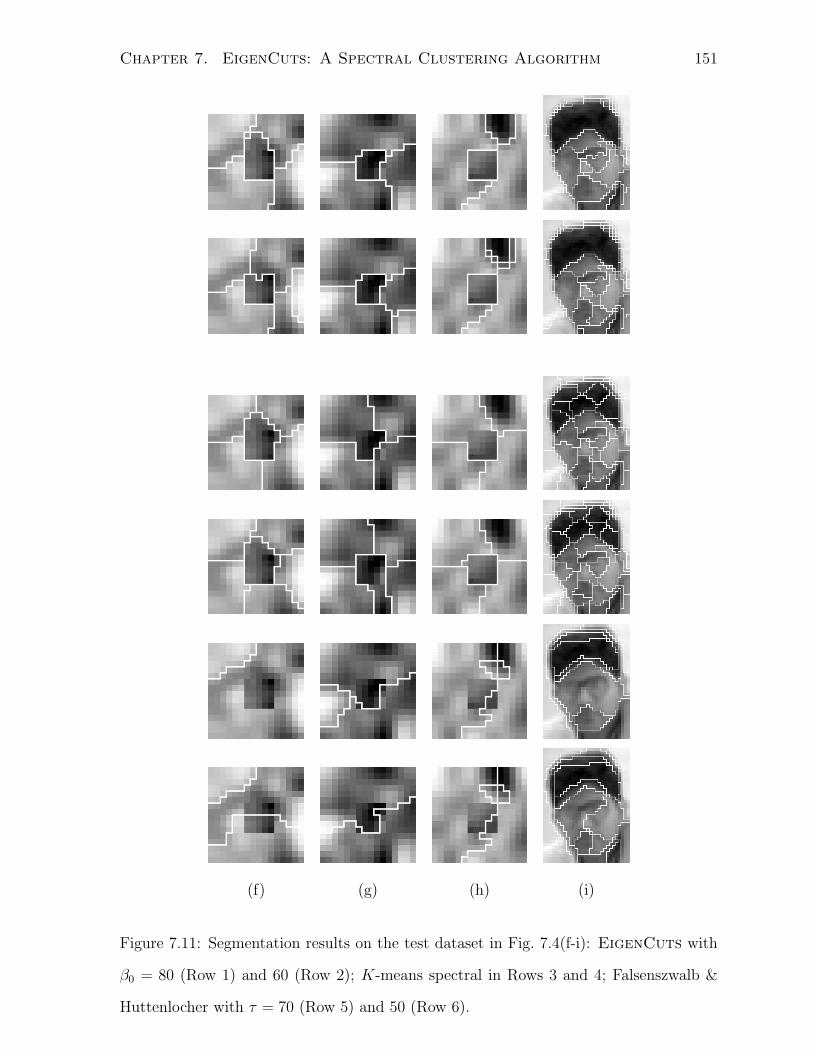
Chapter 7. EigenCuts: A Spectral Clustering Algorithm 151
(f) (g) (h) (i)
Figure 7.11: Segmentation results on the test dataset in Fig. 7.4(f-i): EigenCuts with
β0 = 80 (Row 1) and 60 (Row 2); K-means spectral in Rows 3 and 4; Falsenszwalb &
Huttenlocher with τ = 70 (Row 5) and 50 (Row 6).

Chapter 8
Hierarchical Representation of
Transition Matrices
Spectral methods enable the study of properties global to a dataset, using only local
pairwise similarity measurements between data points. We have studied global properties
that emerge from such similarities in terms of a random walk formulation on the graph.
In particular, as described in Chapter 7, we can partition the graph into clusters by
analyzing the perturbations to the stationary distribution of a Markovian relaxation
process defined in terms of the affinity weights. The Markovian relaxation process need
never be explicitly carried out; instead, it can be analytically expressed using the leading
order eigenvectors, and eigenvalues, of the Markov transition matrix.
Two issues arise in the implementation of spectral methods. First, the stochastic
matrices need not be symmetric in general, and hence for reasons of numerical instability,
a direct eigen decomposition step is not preferred. This problem is easily circumvented
by considering a normalized affinity matrix which is related to the stochastic matrix by
a similarity transformation (Eq. 7.7). By virtue of symmetry, the eigen decomposition
of the normalized symmetric matrix is numerically stable (e.g., see §6.5 [118]). While
the eigenvalues of the stochastic matrix remain the same as for the normalized affinity
152

Chapter 8. Hierarchical Representation of Transition Matrices 153
matrix, the eigenvectors are related by a simple transformation.
The second issue is how the spectral methods scale to large datasets. In particular, the
eigen decomposition can be very expensive, on the order of O(n3), where n = |V |. While
it is possible to compute analytically the first eigenvector (see §7.2.4), the remaining
subspace of vectors necessary for clustering has to be explicitly computed. A typical
approach to dealing with this difficulty is to first sparsify the links in the graph, thus
generating a sparse affinity matrix, and then apply an efficient eigensolver such as Lanczos
[56].
In comparison, we propose in this chapter a specialized eigensolver suitable for large
stochastic matrices with known stationary distributions. In particular, we exploit the
spectral properties of the Markov transition matrix to generate hierarchical, successively
lower-ranked approximations to the full transition matrix. The eigen problem is solved
directly at the coarsest level of representation. The approximate eigen solution is then in-
terpolated over successive levels of the hierarchy, using a small number of power iterations
to correct the solution at each stage. To show the effectiveness of this approximation, we
present a multi-scale version of the EigenCuts algorithm in the subsequent chapter.
8.1 Previous Work
One approach to speeding up the eigen decomposition is to use the fact that the columns
of the affinity matrix are typically correlated. The idea then is to pick a small number
of representative columns to perform eigen decomposition via SVD. For example, in the
Nystrom approximation procedure, originally proposed for integral eigenvalue problems
[31,89], the idea is to randomly pick a small set of m columns; generate the corresponding
affinity matrix; solve the eigenproblem and finally extend the solution to the complete
graph [15,40]. The Nystrom method has also been recently applied in the kernel learning
methods for fast Gaussian process classification and regression [121]. Other sampling-

Chapter 8. Hierarchical Representation of Transition Matrices 154
based approaches include the work reported in [1, 2, 42].
Our starting point is the transition matrix generated from affinity weights and we
show how building a representational hierarchy follows naturally from considering the
stochastic matrix. The work closest in spirit to our research is the paper by Lin on
reduced rank approximations of transition matrices [62]. We differ in how we approx-
imate the transition matrices, in particular our objective function is computationally
less expensive to solve. While the paper by Lin suggests interpreting the reduced rank
approximations directly for clustering, we embed our procedure in a graph partitioning
framework. In particular, one of our goals in reducing transition matrices is to develop a
fast, specialized eigen solver for spectral clustering. Fast eigensolving is also the goal in
ACE [53], where successive levels in the hierarchy can potentially have negative affinities.
A graph coarsening process for clustering was also pursued in [100].
8.2 Markov Chain Terminology
We first provide a brief overview of the Markov chain terminology here (for more details
see §7.2). We consider an undirected graph G = (V,E) with vertices vi, for i = 1, . . . , n,
and edges ei,j with non-negative weights ai,j. Here the weight ai,j represents the affinity
between vertices vi and vj. The affinities are represented by a non-negative, symmetric
n × n matrix A having weights ai,j as elements. The degree of a node j is defined to
be: dj =∑n
i=1 ai,j =∑n
j=1 aj,i, while D is a diagonal matrix of degree values: D =
diag(d1, . . . , dn). A Markov chain is defined using these affinities by setting a transition
probability matrix M = AD−1, where the columns of M each sum to 1. The transition
probability matrix defines the random walk of a particle on the graph G.
For analysis, we consider a similarity transformation of the Markov matrix: L =
D−1/2MD1/2. Observe L is a normalized form of the affinity matrix given by: L =
D−1/2AD−1/2. As a consequence L is symmetric and hence it can be diagonalized as:
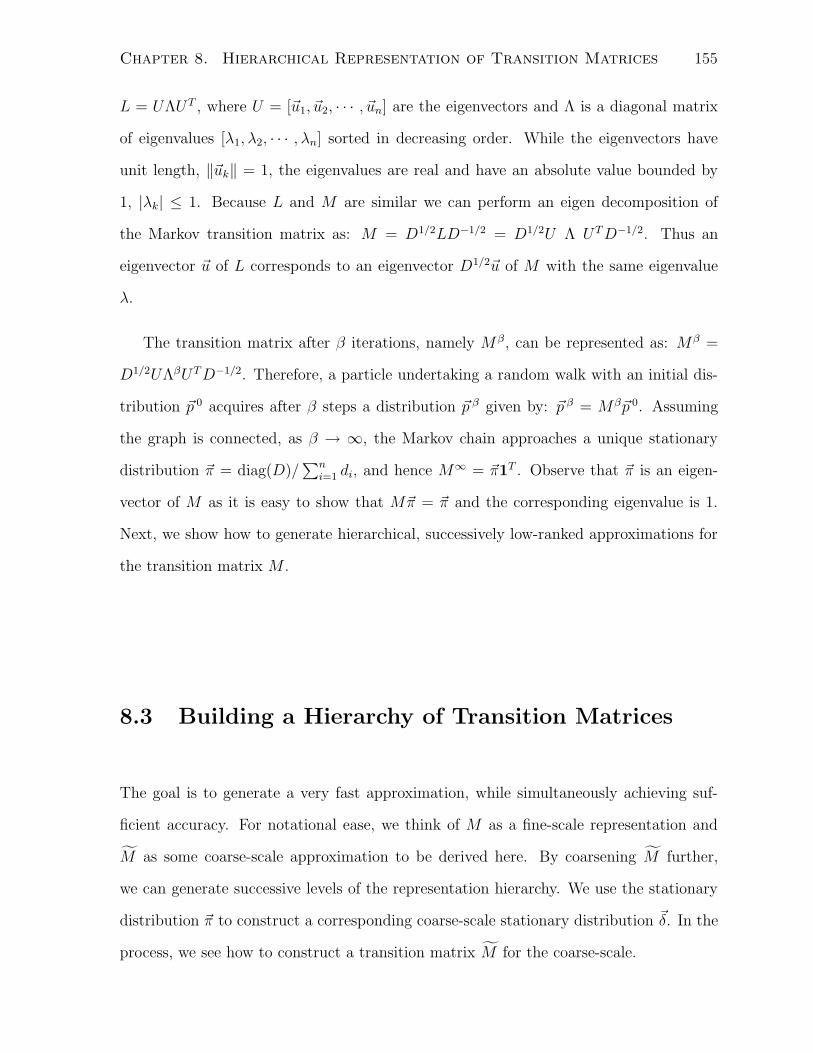
Chapter 8. Hierarchical Representation of Transition Matrices 155
L = UΛUT , where U = [~u1, ~u2, · · · , ~un] are the eigenvectors and Λ is a diagonal matrix
of eigenvalues [λ1, λ2, · · · , λn] sorted in decreasing order. While the eigenvectors have
unit length, ‖~uk‖ = 1, the eigenvalues are real and have an absolute value bounded by
1, |λk| ≤ 1. Because L and M are similar we can perform an eigen decomposition of
the Markov transition matrix as: M = D1/2LD−1/2 = D1/2U Λ UT D−1/2. Thus an
eigenvector ~u of L corresponds to an eigenvector D1/2~u of M with the same eigenvalue
λ.
The transition matrix after β iterations, namely M β, can be represented as: Mβ =
D1/2UΛβUT D−1/2. Therefore, a particle undertaking a random walk with an initial dis-
tribution ~p 0 acquires after β steps a distribution ~p β given by: ~p β = Mβ~p 0. Assuming
the graph is connected, as β → ∞, the Markov chain approaches a unique stationary
distribution ~π = diag(D)/∑n
i=1 di, and hence M∞ = ~π1T . Observe that ~π is an eigen-
vector of M as it is easy to show that M~π = ~π and the corresponding eigenvalue is 1.
Next, we show how to generate hierarchical, successively low-ranked approximations for
the transition matrix M .
8.3 Building a Hierarchy of Transition Matrices
The goal is to generate a very fast approximation, while simultaneously achieving suf-
ficient accuracy. For notational ease, we think of M as a fine-scale representation and
M as some coarse-scale approximation to be derived here. By coarsening M further,
we can generate successive levels of the representation hierarchy. We use the stationary
distribution ~π to construct a corresponding coarse-scale stationary distribution ~δ. In the
process, we see how to construct a transition matrix M for the coarse-scale.

Chapter 8. Hierarchical Representation of Transition Matrices 156
8.3.1 Deriving Coarse-Scale Stationary Distribution
We begin by expressing the stationary distribution ~π as a probabilistic mixture of latent
distributions. In matrix notation, we have
~π = K~δ, (8.1)
where ~δ is an unknown mixture coefficient vector of length m, K is an n×m non-negative
kernel matrix whose columns are latent distributions that each sum to 1 and m n.
For choosing the kernels K, we first diffuse the Markov matrix M using a small
number of iterations to get Mβ. The diffusion causes random walks from neighboring
nodes to be less distinguishable. We then choose a small number of columns of M β to
be the kernel matrix K1. The kernel selection is fast and greedy; we defer the details to
the following section.
We now show how to get a maximum likelihood approximation of ~δ using an EM type
algorithm [71]. To derive this we minimize the Kullback-Liebler distance measure [54,55]
between the two probability distributions ~π and K~δ given by
L = −n∑
i=1
πi ln
∑mj=1 Ki,jδj
πi
,
= −n∑
i=1
πi lnm∑
j=1
Ki,jδj +∑
i
πi ln πi. (8.2)
Note the second term in the above expression is the negative entropy of the station-
ary distribution ~π. Given that ~δ is a probability distribution, a maximum likelihood
estimating process has to find a stationary point(~δ, λ)
for the following Lagrangian
E = L + λ
( m∑
j=1
δj − 1
),
= −n∑
i=1
πi lnm∑
j=1
Ki,jδj + λ
( m∑
j=1
δj − 1
), (8.3)
1If M is a full matrix, to avoid the expense of computing Mβ explicitly, random kernel centers can
be selected, and only the corresponding columns of Mβ need be computed.

Chapter 8. Hierarchical Representation of Transition Matrices 157
where the negative entropy term∑
i πi ln πi in L is dropped because it will have a fixed
value and hence will not affect the subsequent minimization with respect to δj. Now,
taking the derivative with respect to δj gives
∂E
∂δj
=n∑
i=1
πiKi,j∑mk=1 δkKi,k
− λ. (8.4)
Setting ∂E∂δj
to zero we obtain
n∑
i=1
πiKi,j∑mk=1 δkKi,k
= λ. (8.5)
Multiplying both sides of the above equation by δj results in
n∑
i=1
πiδjKi,j∑mk=1 δkKi,k
= λδj. (8.6)
Because the contribution made by kernel j at node i is given by Ki,j, we can define
ownership of a node i by kernel j as
ri,j =δjKi,j∑m
k=1 δkKi,k
. (8.7)
Using the ownerships ri,j we can rewrite Eq. 8.6 as
n∑
i=1
πiri,j = λδj. (8.8)
By definition∑m
j=1 ri,j = 1 and hence we have
n∑
i=1
m∑
j=1
πiri,j = λm∑
j=1
δj,
n∑
i=1
πi = λ,
⇒ λ = 1. (8.9)
Here we use the fact that∑m
j=1 δj = 1 and∑n
i=1 πi = 1. Substituting for λ in Eq. 8.8 gives
the mixing probability, which is the stationary distribution at the coarse-scale, given by
δj =n∑
i=1
πiri,j . (8.10)

Chapter 8. Hierarchical Representation of Transition Matrices 158
Along with ~δ, we can update the latent distributions in the kernel matrix K (as
in [62]). To see how notice that we can interpret the responsibility term ri,j in Eq. 8.10
as the conditional probability of being in the coarse-scale node j given the fine scale state
i. Hence, in Eq. 8.10 we are integrating over the states at the fine-scale, each having a
probability πi, so we can obtain the coarse-scale distribution ~δ. Similarly, elements in the
kernel matrix Ki,j represent the conditional probability of being in fine-scale state i given
the coarse-scale state j. Then using Bayes theorem the kernel matrix can be updated as
follows:
Ki,j =ri,jπi
δj
, (8.11)
where we use the updated coarse-scale stationary distribution values from Eq. 8.10. Thus,
a EM type procedure would follow this sequence of steps:
1. M-step
• Compute ownership maps ri,j (Eq. 8.7)
2. E-step
• Estimate mixing probabilities which are the coarse-scale stationary distribu-
tion values δj (Eq. 8.10)
• Estimate the kernel parameters Ki,j (Eq. 8.11)
3. Repeat until convergence
By diffusing the Markov matrix M through a small number of iterations, as in M β, and
then choosing a small number of columns of Mβ as the kernel matrix K, we facilitate a
rapid convergence of the EM procedure. We initialize ~δ to be uniform over the coarse-
scale states.

Chapter 8. Hierarchical Representation of Transition Matrices 159
8.3.2 Deriving the Coarse-Scale Transition Matrix
In order to define M , we break it down into two steps. To define the random walk in the
reduced space, say
~q k+1 = M~q k, (8.12)
we first expand ~q k into the fine scale using the kernels K, resulting in
~p k = K~q k. (8.13)
Then we lift ~p k back into the coarse scale by using the ownership probability of the
jth kernel for the ith node on the fine grid. Computing the ownership probability is an
implicit step in the EM procedure described above and is given by
ri,j =δjKi,j∑m
k=1 δkKi,k
.
Thus,
q k+1j =
n∑
i=1
ri,jpki ,
=n∑
i=1
ri,j
m∑
t=1
Ki,tqk
t ,
=n∑
i=1
(δjKi,j∑m
k=1 δkKi,k
) m∑
t=1
Ki,tqk
t . (8.14)
We can write the preceding equation in a matrix form,
~q k+1 = diag(~δ ) KT diag(K~δ)−1
K~q k, (8.15)
= M~q k,
where the transition matrix is given by
M = diag(~δ ) KT diag(K~δ)−1
K. (8.16)
It is easy to see that ~δ = M~δ, so ~δ is the stationary distribution for M .

Chapter 8. Hierarchical Representation of Transition Matrices 160
One critical property of the fine scale Markov matrix that we would like to preserve
in the coarse scale version is that it is precisely similar to a symmetric matrix. It follows
from the definition of M and its stationary distribution ~δ, we can generate a scaled
symmetric affinity matrix A given by
A = γMdiag(~δ), (8.17)
= γ(diag(~δ ) KT
)(diag
(K~δ)−1)(
Kdiag(~δ))
,
where we substitute for the transition matrix M from Eq. 8.16. From this equation, it is
clear that the affinity matrix at coarse-scale is also symmetric. The scalar variable γ is
used to fix the scale by computing
γ−1 = median(di), (8.18)
where di is the degree of node i in the coarse-scale graph represented by the matrix A
(as in step 2 of Sec. 7.4). The coarse-scale affinity matrix A is normalized to get
D = diag(d1, d2, · · · , dm),
L = D−1/2AD−1/2. (8.19)
which is then used for eigen decomposition.
To summarize, we use the stationary distribution ~π at the fine-scale to derive a tran-
sition matrix M , and its stationary distribution ~δ, at the coarse-scale. It is obvious that
this procedure can be repeated recursively. To maintain consistency, a γ factor is com-
puted for each level of the hierarchy and the corresponding affinity matrix is scaled. Also,
at successive levels of the hierarchy we sparsify A by zeroing out elements associated with
small transition probabilities in M .
8.3.3 Selecting Kernels
In Fig. 8.1, we show the details of kernel selection for a three-scale approximation of the
transition matrix, one fine-scale and two coarse-scales. To begin with, a graph cluster-

Chapter 8. Hierarchical Representation of Transition Matrices 161
1
2
3
4
5
6
7
8
9
10
11
12
13
14
15
16
17
18
19
20
21
22
23
24
25
26
27
28
29
30
31
32
33
34
35
36
37
38
39
40
1
2
3
4
5
6
7
8
9
10
11
12
13
14
15
16
17
1
2
3
4
5
6
7
8
9
10
11
12
13
14
15
16
17
18
19
2021
22
23
24
2526
27
28
29
30
31
32
33
34
35
3637
38
39
40
41
4243
44
45
46
47
4849
50
51
52
53
54
55
56
57
5859
60
61
62
63
64
65
66
6768
6970
71
72
73
74
7576
77
78
79
8081
82
83
1
2
3
4
5
6
7
8 9
10
11
12
13
14
15
16
17
18
19
20
21
22
23
24
25
26
27
28
29
30
31
32
Kernel centers for scale 1 Kernel centers for scale 2
Figure 8.1: Kernel selection at levels 2 (Left Column) and 3 (Right Column) of the
hierarchy. The numbers in red and magenta indicate the location of the kernel centers.
Figure 8.2: A random selection of kernels for the occluder image. These kernels carry
information from fine-scale (level 1) to the first coarse-scale (level 2) of the hierarchy.
The kernel matrix is of size 256× 40.
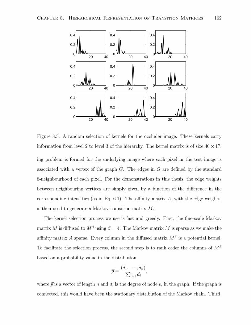
Chapter 8. Hierarchical Representation of Transition Matrices 162
20 400
0.2
0.4
20 400
0.2
0.4
20 400
0.2
0.4
20 400
0.2
0.4
20 400
0.2
0.4
20 400
0.2
0.4
20 400
0.2
0.4
20 400
0.2
0.4
20 400
0.2
0.4
Figure 8.3: A random selection of kernels for the occluder image. These kernels carry
information from level 2 to level 3 of the hierarchy. The kernel matrix is of size 40× 17.
ing problem is formed for the underlying image where each pixel in the test image is
associated with a vertex of the graph G. The edges in G are defined by the standard
8-neighbourhood of each pixel. For the demonstrations in this thesis, the edge weights
between neighbouring vertices are simply given by a function of the difference in the
corresponding intensities (as in Eq. 6.1). The affinity matrix A, with the edge weights,
is then used to generate a Markov transition matrix M .
The kernel selection process we use is fast and greedy. First, the fine-scale Markov
matrix M is diffused to Mβ using β = 4. The Markov matrix M is sparse as we make the
affinity matrix A sparse. Every column in the diffused matrix M β is a potential kernel.
To facilitate the selection process, the second step is to rank order the columns of M β
based on a probability value in the distribution
~p =(d1, · · · , dn)∑n
i=1 di
,
where ~p is a vector of length n and di is the degree of node vi in the graph. If the graph is
connected, this would have been the stationary distribution of the Markov chain. Third,

Chapter 8. Hierarchical Representation of Transition Matrices 163
the kernels (i.e. columns of Mβ) are picked in such a way that for a kernel Ki all of
its neighbours which are within the half-height of its peak value are suppressed from the
selection process. Finally, the kernel selection is continued until we ensure that every
pixel in the image is within a half-height of the peak value of at least one kernel.
We show results from a three-scale hierarchy in Fig. 8.1, where the left, and right,
columns indicate the locations of the kernel centers for two different images at the two
coarse-scales. The random occluder image is of size 16 × 16 pixels and the eye image
is of size 25 × 20 pixels. These images are enlarged in Fig. 8.1 for clarity. For the
random occluder image, the greedy algorithm picks 40 kernels which allow us to go from
from scale 1 (fine-scale) to scale 2 (coarse-scale) of the hierarchy. The kernel centers are
shown in numbers. The transition matrix M generated for the 40 dimensional space is
then diffused to Mβ, again using β = 4. The greedy algorithm is applied again, this
time picking 17 kernels, which allow us to go from scale 2 to scale 3 of the hierarchy.
Similar results can be seen for the eye image. In Fig. 8.2, we show a random sample
of kernels. The kernels are columns of the transition matrix and hence, they should be
seen as conditional probability distributions. Note, at higher levels of the hierarchy, the
kernel matrix begins to get less sparse. Consequently, the corresponding affinity matrix
will be less sparse as well (see Fig. 8.3). We next describe how to use this representation
hierarchy for building a fast eigensolver.
8.4 Fast EigenSolver
Given that our procedure is hierarchical, the eigen decomposition of the normalized
affinity matrix L is done only at the “coarsest” scale. Once computed, the coarse-
scale eigenvectors are interpolated using the kernel matrix to generate the fine-scale
eigenvectors. For demonstration purposes, let us consider a three-scale interpolation
process applied to the test image of an eye (Fig. 8.1). The first scale is the fine-scale

Chapter 8. Hierarchical Representation of Transition Matrices 164
normalized affinity matrix L for the eye image and is of size n× n where n = 500. The
kernel selection selection process results in a matrix K, which is of size n × m where
m = 83 and m is typically n. The coarse-scale representation of L at the second level
of the hierarchy is L, which is of size m×m. This representation is further reduced at the
third-level of the hierarchy to a matrix of size e× e, which for the face image is 32× 32.
A full eigen decomposition of the normalized affinity matrix is done only at the
coarsest level. As discussed in the previous section the affinity matrix at the coarsest
level is not likely to be sparse, hence it will need a full (as opposed to a sparse) version
of an eigen solver. However it is typically the case that e ≤ m n, even in the case
of the three-scale hierarchy that is under consideration. The resulting eigenvectors are
interpolated to the next lower level of the hierarchy by a process which will be described
next. Because the eigen interpolation process between every adjacent pair of scales in the
hierarchy is similar, we will assume we have access to the leading eigenvectors U (size:
m× e) for the normalized affinity matrix L (size: m×m) and describe how to generate
the leading eigenvectors U (size: n× e), and leading eigenvalues S (size: e× 1), for the
fine-scale normalized affinity matrix L (size: n× n). There are several steps to the eigen
interpolation process.
• First, the coarse-scale eigenvectors U can be interpolated using the kernel matrix
K to generate U , an approximation for the fine-scale eigenvectors,
U = KU.
• Second, interpolation alone is unlikely to set the directions of U exactly aligned
with UL, the vectors one would obtain by a direct eigen decomposition of the fine-
scale normalized affinity matrix L. We update the directions in U by applying a
small number of power iterations with L as in:
for i = 1 to POWER ITERS do
U ⇐ LU

Chapter 8. Hierarchical Representation of Transition Matrices 165
end for
• Third, the interpolation process and the power iterations need not preserve orthog-
onality in the eigenvectors in U . We fix this by Gram-Schmidt orthogonalization
procedure.
• Finally, there is a still a problem with power iterations that needs to be resolved,
in that it is very hard to separate nearby eigenvalues. In particular, for the conver-
gence of the power iterations the ratio that matters is between the (e+1)st and eth
eigenvalues. So the idea we pursue is to use the power iterations only to separate
the reduced space of eigenvectors (of dimension e) from the orthogonal subspace
(of dimension n− e). We then use a full SVD on the reduced space to update the
leading eigenvectors U , and eigenvalues S, for the fine-scale:
Le = UT LU,
UeSeVTe = svd(Le),
U ⇐ UUTe ,
S ⇐ diag(Se).
In Algorithm 2 we present the details of this coarse to fine eigen interpolation proce-
dure.
8.4.1 Interpolation Results
In Fig. 8.4 we compare the spectrum S obtained from a three-scale decomposition on
the eye and face images (Fig. 7.4) with the ground truth, which is the spectrum SL
resulting from direct eigen decomposition of the fine-scale normalized affinity matrices
L. For the direct eigen decomposition, we have used the Matlab implementation of an
implicitly restarted Arnoldi method for solving large-scale eigenvalue problems [90]. Our
multi-scale decomposition code is also in Matlab.

Chapter 8. Hierarchical Representation of Transition Matrices 166
Algorithm 2 function (U, S) = CoarseToFine(L,K, U)
1: INPUT
2: L,K ⇐ L is n× n and K is n×m where m n
3: U ⇐ leading coarse-scale eigenvectors of L. U is of size m× e, e ≤ m
4: OUTPUT
5: U, S ⇐ leading fine-scale eigenvectors/eigenvalues of L. U is n×e and S is e×1.
6: CONSTANTS
7: TOL = 1.0e−3; POWER ITERS = 25
8:
9: U = KU interpolation from coarse to fine
10: while not converged do
11: Uold = U n× e matrix, e n
12: for i = 1 to POWER ITERS do
13: U ⇐ LU
14: end for
15: U ⇐ Gram-Schmidt(U) orthogonalize U
16: Le = UT LU L may be sparse, but Le need not be.
17: UeSeUTe = svd(Le) eigenanalysis of Le, which is of size e× e.
18: U ⇐ UUe update the leading eigenvectors of L
19: S = diag(Se) grab the leading eigenvalues of L
20: innerProd = 1− diag( UTold U ) 1 is a e× 1 vector of all ones
21: converged = max[abs(innerProd)] < Tol
22: end while

Chapter 8. Hierarchical Representation of Transition Matrices 167
5 10 15 20 25 30
0.88
0.9
0.92
0.94
0.96
0.98
1
Eigen Index
Eig
en V
alue
Eigen Spectrum
5 10 15 20 25 30
0.5
1
1.5
2
2.5
3
x 10−3
Eigen Index
Abs
olut
e R
elat
ive
Err
or
|δλ|λ−1
20 40 60 80 100
0.88
0.9
0.92
0.94
0.96
0.98
Eigen Index
Eig
en V
alue
Eigen Spectrum
20 40 60 80 100
0.005
0.01
0.015
0.02
0.025
Eigen Index
Abs
olut
e R
elat
ive
Err
or|δλ|λ−1
Figure 8.4: Hierarchical eigensolver applied to the eye image (Top Row) and the face
image (Bottom Row). Comparison of eigen spectra: red circles represent the eigen-
values SL obtained by a direct eigen decomposition of the fine-scale normalized affinity
matrix L; blue line with crosses are eigenvalues S obtained by a three-scale decomposi-
tion of the transition matrix built from L. Plots to the right show the relative absolute
error: |S−SL|SL
, between the eigenvalues.
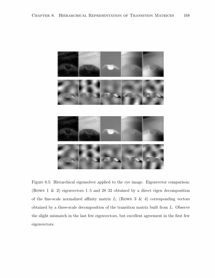
Chapter 8. Hierarchical Representation of Transition Matrices 168
Figure 8.5: Hierarchical eigensolver applied to the eye image. Eigenvector comparison:
(Rows 1 & 2) eigenvectors 1–5 and 28–32 obtained by a direct eigen decomposition
of the fine-scale normalized affinity matrix L; (Rows 3 & 4) corresponding vectors
obtained by a three-scale decomposition of the transition matrix built from L. Observe
the slight mismatch in the last few eigenvectors, but excellent agreement in the first few
eigenvectors.

Chapter 8. Hierarchical Representation of Transition Matrices 169
5 10 15 20 25 30
0.05
0.1
0.15
0.2
0.25
0.3
0.35
0.4
Eigen Index
Rel
ativ
e E
rror
20 40 60 80 100
0.1
0.2
0.3
0.4
0.5
0.6
0.7
0.8
0.9
Eigen Index
Rel
ativ
e E
rror
Figure 8.6: Measuring the mismatch: 1 − diag(|UT UL|
), between the eigenvectors U
derived from multi-scale approximation and the ground truth UL for the eye image (Left)
and the face image (Right).
For the eye image, recall the original Markov matrix is of size 500 × 500, which is
reduced to a 83×83 matrix at the second level of the hierarchy and is further reduced to a
matrix of size 32×32 at the third level of the hierarchy. Hence the eigenspectrum is a 32-
long vector (Fig. 8.4 Top Left). To illustrate how close the multi-scale approximation
is to the true eigen spectrum we show absolute relative error between the spectra: |S−SL|SL
(Fig. 8.4, Top Right). The spectra agree mostly, except for the last few eigenvalues.
Similar results can be seen for the face image, where the fine-scale affinity matrix is
of size 1200× 1200, which is reduced to a matrix of size 252× 252 at the second-level of
the hierarchy and further reduced to a matrix of size 111× 111 at the third-level of the
hierarchy. Hence, the eigenspectrum is a 111 long vector as shown in Fig. 8.4 (Bottom
Left). The absolute relative error demonstrates a close match between the multi-scale
approximation and the ground truth, in the leading eigenvalues.
To further assess the mis-match between the spectra, in Fig. 8.5 we compare visually
the leading eigenvectors for the eye image returned by the multi-scale approximation to
the ground truth. The first two rows of the figure correspond to the first and the last

Chapter 8. Hierarchical Representation of Transition Matrices 170
10 20 30 40 50 60 70
2
4
6
8
10
12
14
16x 10
−3
Eigen Index
Abs
Rel
Err
in E
igen
Val
s
10 20 30 40 50 60 70
0.1
0.2
0.3
0.4
0.5
0.6
0.7
0.8
0.9
Eigen Index
Rel
Err
in E
igen
vect
ors
10 20 30 40 50
2
4
6
8
10x 10
−3
Eigen Index
Abs
Rel
Err
in E
igen
Val
s
10 20 30 40 50
0.1
0.2
0.3
0.4
0.5
0.6
0.7
0.8
0.9
Eigen Index
Rel
Err
in E
igen
vect
ors
5 10 15 20 25 30
0.5
1
1.5
2
2.5
3
3.5
x 10−3
Eigen Index
Abs
Rel
Err
in E
igen
Val
s
5 10 15 20 25 30
0.1
0.2
0.3
0.4
0.5
0.6
0.7
0.8
0.9
Eigen Index
Rel
Err
in E
igen
vect
ors
Figure 8.7: Hierarchical eigensolver on the face image for various subspace dimensions:
(Top Row) 71, (Middle Row) 51 and (Bottom Row) 31. (Left Column) Rela-
tive absolute error: |S−SL|SL
, between the eigenvalues S returned by the eigensolver and
the ground-truth SL. (Right Column) Measuring the mismatch: 1 − diag(|UT UL|
),
between the eigenvectors U derived from multi-scale approximation and the ground truth
UL.

Chapter 8. Hierarchical Representation of Transition Matrices 171
five eigenvectors returned by a direct eigen decomposition of the fine-scale normalized
affinity matrix L. The third and fourth rows show the corresponding eigenvectors from
the multi-scale procedure. Notice the last few eigenvectors exhibit a slight mismatch.
For a quantitative comparison, in Fig. 8.6 we plot the following measure to indicate
how good the approximation is to the ground-truth: 1−|U T UL|, where 1 is a vector of all
ones, U is the matrix of eigenvectors obtained by the multi-scale approximation and UL
is the ground-truth resulting from a direct eigen decomposition of the fine-scale affinity
matrix L. The relative error plot demonstrates a close match in the leading eigenvector
directions between the two methods. The relative error is high with the last few eigen
vectors, which suggests that the power iterations have not clearly separated them from
other directions.
Finally, we compare the timings of the two eigensolvers: the sparse SVD routine
mentioned before [90] and our hierarchical method. In Table. 8.1 using a three-scale
decomposition of the face image, we report time taken, in seconds, to compute the leading
eigenbasis for a fixed size input problem. We consider the face image, where the fine-scale
affinity matrix is of size 1200 × 1200, which is reduced to a matrix of size 252 × 252 at
the second-level of the hierarchy and further reduced to a matrix of size 111 × 111 at
the third-level of the hierarchy. Given the matrix size at the coarsest scale, we have an
option to pick the total number of eigenbases to be interpolated down the hierarchy. So,
in Table 8.1 we report the time it takes to compute the leading eigenbasis for various
subspace dimensionalities. Also for each subspace selection, the sparse SVD procedure
is invoked for the corresponding basis on the fine-scale sparse normalized affinity matrix.
The results from the sparse SVD routine serve as the ground-truth.
Comparing the numbers in Table. 8.1, the multi-scale approach clearly outperforms
the sparse SVD routine. However, as we observed before the relative error between the
interpolated eigen vectors from the multi-scale procedure and the sparse SVD basis tends
to be high in the last few eigen directions (see Figs. 8.6 and 8.7). The strategy we suggest

Chapter 8. Hierarchical Representation of Transition Matrices 172
Eigen Subspace Dim Sparse SVD Multi-Scale Approach
11 21.1 2.9
31 55.3 3.4
51 90.4 3.8
71 127.3 4.4
91 171.1 5.5
111 220.5 6.3
Table 8.1: Comparing the timings of the two eigensolvers on a 1200 × 1200 Markov
matrix: Sparse SVD [90] and the hierarchical approach reported in this chapter, where
the size of the input problem is fixed but the the size of the leading subspace is changed.
The reported time is in seconds. The code, written in Matlab, is run on a Pentium 4,
1.9Ghz, 512MB machine.
Image Size Markov Matrix Size Sparse SVD Multi-Scale Approach
16× 16 [2562 392] 4.2 0.6
24× 24 [5762 852 322] 12.1 1.3
32× 32 [10242 1502 562] 28.3 4.7
48× 48 [23042 3342 1202 482] 95.6 8.9
64× 64 [40962 5732 2132 712] 271.9 35.0
Table 8.2: Comparing the timings of the two eigensolvers: Sparse SVD [90] and the
hierarchical approach reported in this chapter, where the size of the input problem is
changed but the size of the leading subspace is kept fixed to a value = 31. The second
columns shows the size of the transition matrix at each level of the hierarchy. The number
of stages in the hierarchy is chosen to accommodate a subspace of atleast 31 dimensions.
The reported time is in seconds. The code, written in Matlab, is run on a Pentium 4,
1.9Ghz, 512MB machine.

Chapter 8. Hierarchical Representation of Transition Matrices 173
then is to pad the required number of leading eigen basis by about 20% before invoking
the multi-scale procedure. Obviously, the number of hierarchical stages for the multi-
scale procedure must be chosen such that the transition matrix at the coarsest scale can
accommodate the slight increase in the subspace dimensions.
Next, we measure the time it takes to compute the leading eigenbasis for various sizes
of the input problem. We form images, each of size N × N , by Gaussian smoothing of
i.i.d noise. The Gaussian function has a standard deviation of 3 pixels. The affinities
are computed as in Eq. 6.1. The affinity matrix is then normalized so that the median
value for the degree di of any node i in the underlying graph is 1 (see Sec. 7.4 for more
discussion). We fix the subspace dimensionality to 31. In Table. 8.2 the column under
sparse SVD denotes the time taken by the sparse SVD routine to generate the leading
31 eigenvectors and eigenvalues. The reported time is in seconds.
We then perform a hierarchical decomposition of the Markov transition matrix. The
number of hierarchical stages is selected to accommodate a minimum subspace of 31
dimensions. In Table. 8.2 the column reporting Markov matrix sizes shows the size of
the transition matrix at each level of the hierarchy and also the number of stages in
the hierarchy. For example, for N = 16 we chose only 2 levels in the hierarchy while
for N = 64 we select 4 levels in the hierarchy. At the coarsest scale a subspace size
that is at most 51 dimensional is selected for interpolation. This conforms to our earlier
suggestion of padding the necessary subspace, which is 31, by a number that is 20%
larger, to overcome the errors introduced by the multi-scale procedure in the last few
eigen directions. Again, the multi-scale procedure outperforms the sparse SVD routine.
In Table 8.2, we suspect the timings reported for N = 64 are an anomaly in that Matlab
is probably hitting an hardware issue with paging or caching. Otherwise, the reported
times for the multi-scale procedure scale linearly in N .

Chapter 9
Multi-Scale EigenCuts
9.1 Introduction
We show how to use the information in the transition matrix approximation hierarchy
to build an effective multi-scale spectral clustering algorithm. In particular, we modify
the basic procedure of EigenCuts for the multi-scale version. At the coarsest scale
we run one iteration of the EigenCuts algorithm. Once the cuts have been identified
at the coarsest scale, processing continues to the next finer scale. The eigenvectors are
interpolated according to the Algorithm 2 presented in Chapter 8, the cut locations
are predicted from the coarser scale and the fine scale sensitivities are computed only at
these locations. We discuss the details of this multi-scale EigenCuts algorithm next.
9.2 Algorithm Details
To begin, a graph clustering problem is formed for the underlying image where each pixel
in the test image is associated with a vertex on the graph G. The edges in G are defined
by the standard 8-neighbourhood of each pixel. The edge weights between neighbouring
vertices are simply given by a function of the difference in the corresponding intensities
(as in Eq. 6.1). The affinity matrix A, with the edge weights, is then used to generate a
174

Chapter 9. Multi-Scale EigenCuts 175
Markov transition matrix M .
We now illustrate the various steps of a three-scale EigenCuts algorithm applied to
a random occluder image shown in Fig. 9.1. The image size is 16 × 16, but is enlarged
in the figures for clarity. The fine-scale Markov matrix M is diffused to M β using β = 4
and a greedy kernel selection process is applied (see §8.3.3). The greedy algorithm picks
40 kernels. The kernel centers are numbered in Fig. 9.1a. The transition matrix M
generated for the 40 dimensional space is then diffused to Mβ, again using β = 4. The
greedy kernel selection algorithm is applied again, this time picking 17 kernels. The
kernel centers are shown in Fig. 9.1b.
At the coarsest scale we run one iteration of the EigenCuts algorithm (§7.4). The
cuts identified at the coarsest scale are drawn as black lines in Fig. 9.1, where a line
joining two kernels indicates a link that is highly sensitive at the coarsest scale and hence
must be cut. Once the cuts have been identified at the coarsest scale, processing continues
to the next finer scale. The eigenvectors are interpolated according to the Algorithm 2
presented in Chapter 8, the cut locations are predicted from the coarser scale and the
fine scale sensitivities are computed only at these locations.
The cut locations at the fine-scale are predicted in a greedy fashion. For illustration,
consider the link between kernels 11 and 18 in Fig. 9.1a, which the EigenCut procedure,
applied at the coarse-scale, identifies as a link to be cut. The kernels will have a form
shown in Fig. 8.2. The greedy method we adopt is to intersect the two kernel shapes and
find pixels with non-zero transition probability between the two kernel centers. From
the Fig. 9.1a, we can see that for kernels 11 and 18, there are six such pixel locations,
drawn as yellow coloured crosses. These pixels (along with their links at the fine-scale)
are then identified for further processing. Note, while we predict cut locations, it may be
more appropriate to predict the actual links that should be perturbed at the fine scale.
Instead we chose a greedy approach for this problem.
As we discussed in §8.3.2, at successive levels of the hierarchy we sparsify the affinity

Chapter 9. Multi-Scale EigenCuts 176
matrix A by zeroing out elements associated with small transition probabilities in M .
The suppression can give rise to the following situation. Consider a link with a non-zero
transition probability at the fine-scale between nodes vi and vj. Assume two different
kernels Kr and Ks have the “maximum” ownership weights (via Eq. 8.7) for nodes vi
and vj respectively. If on account of suppression, which happens before the EigenCuts
procedure is run, the transition probability between coarse-scale nodes vcr and vc
s is zero,
then this information must be propagated to the fine-scale for further investigation. In
Fig. 9.1a these links are identified by blue colored lines and they form part of the set of
predicted cut locations.
The actual cuts are made only at the finest scale and the process by which this is
done was already explained in Sec. 7.4.1. The weights of the links that are cut, are
moved into the diagonal of the affinity matrix A at the finest scale, as is done in the
basic EigenCuts procedure.
In Figs. 9.1 to 9.5 we show successive iterations of this multi-scale procedure. In
the first iteration shown in Fig. 9.1, we see that the multi-scale EigenCuts algorithm
eliminates large portions of the image from further analysis. Interestingly, the majority
of the blue lines are at the boundary of the foreground object and this confirms our
intuition that the links across the boundary are weak and hence they are being suppressed
indirectly at a coarser scale. In the second iteration (Fig. 9.2), the placement of kernels
is roughly the same. Notice, at the third-level of the hierarchy (Fig. 9.2b) an extra kernel
(labeled ’8’) is placed inside the foregound object, when compared to the configuration
in the previous iteration. As more links get cut, more kernels are placed inside the
foreground and background regions. For the image used in this demonstration, the multi-
scale algorithm converges after the fifth iteration.
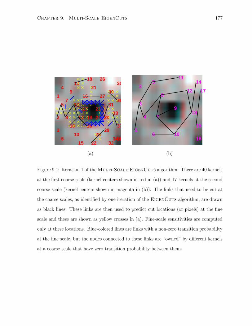
Chapter 9. Multi-Scale EigenCuts 177
1
2
3
4
5
6
7
8
9
10
11
12
13
14
15
16
17
18
19
20
21
22
23
24
25
26
27
28
29
30
31
32
33
34
35
36
37
38
39
40
1
2
3
4
5
6
7
8
9
10
11
12
13
14
15
16
17
(a) (b)
Figure 9.1: Iteration 1 of the Multi-Scale EigenCuts algorithm. There are 40 kernels
at the first coarse scale (kernel centers shown in red in (a)) and 17 kernels at the second
coarse scale (kernel centers shown in magenta in (b)). The links that need to be cut at
the coarse scales, as identified by one iteration of the EigenCuts algorithm, are drawn
as black lines. These links are then used to predict cut locations (or pixels) at the fine
scale and these are shown as yellow crosses in (a). Fine-scale sensitivities are computed
only at these locations. Blue-colored lines are links with a non-zero transition probability
at the fine scale, but the nodes connected to these links are “owned” by different kernels
at a coarse scale that have zero transition probability between them.

Chapter 9. Multi-Scale EigenCuts 178
1
2
3
4
5
6
7
8
9
10
11
12
13
14
15
16
17
18
19
20
21
22
23
24
25
26
27
28
29
30
31
32
33
34
35
36
37
38
39
40
1
2
3
4
5
6
7
8 9
10
11
12
13
14
15
16
17
(a) (b)
Figure 9.2: Iteration 2 of the Multi-Scale EigenCuts algorithm. There are 40 kernels
at the first coarse scale (kernel centers shown in red in (a)) and 17 kernels at the second
coarse scale (kernel centers shown in magenta in (b)). The links that need to be cut at
the coarse scales, as identified by one iteration of the EigenCuts algorithm, are drawn
as black lines. These links are then used to predict cut locations (or pixels) at the fine
scale and these are shown as yellow crosses in (a). Fine-scale sensitivities are computed
only at these locations. Blue-colored lines are links with a non-zero transition probability
at the fine scale, but the nodes connected to these links are “owned” by different kernels
at a coarse scale that have zero transition probability between them.

Chapter 9. Multi-Scale EigenCuts 179
1
2
3
4
5
6
7
8
9
10
11
12
13
14
15
16
17
18
19
20
21
22
23
24
25
26
27
28
29
30
31
32
33
34
35
36
37
38
39
40
1
2
3
4
5
6
7
8 9
10
11
12
13
14
15
16
17
(a) (b)
Figure 9.3: Iteration 3 of the Multi-Scale EigenCuts algorithm. There are 40 kernels
at the first coarse scale (kernel centers shown in red in (a)) and 17 kernels at the second
coarse scale (kernel centers shown in magenta in (b)). The links that need to be cut at
the coarse scales, as identified by one iteration of the EigenCuts algorithm, are drawn
as black lines. These links are then used to predict cut locations (or pixels) at the fine
scale and these are shown as yellow crosses in (a). Fine-scale sensitivities are computed
only at these locations. Blue-colored lines are links with a non-zero transition probability
at the fine scale, but the nodes connected to these links are “owned” by different kernels
at a coarse scale that have zero transition probability between them.

Chapter 9. Multi-Scale EigenCuts 180
1
2
3
4
5
6
7
8
9
10
11
12
13
14
15
16
17
18
19
202122
23
24
25
26
27
28
29
30
31
32
33
34
35
36
37
38
39
40
41
42
1
2
3
4
5
6
7
8
9 10
11
12
13
14
15
16
17
18
19
(a) (b)
Figure 9.4: Iteration 4 of the Multi-Scale EigenCuts algorithm. There are 42 kernels
at the first coarse scale (kernel centers shown in red in (a)) and 19 kernels at the second
coarse scale (kernel centers shown in magenta in (b)). The links that need to be cut at
the coarse scales, as identified by one iteration of the EigenCuts algorithm, are drawn
as black lines. These links are then used to predict cut locations (or pixels) at the fine
scale and these are shown as yellow crosses in (a). Fine-scale sensitivities are computed
only at these locations. Blue-colored lines are links with a non-zero transition probability
at the fine scale, but the nodes connected to these links are “owned” by different kernels
at a coarse scale that have zero transition probability between them.

Chapter 9. Multi-Scale EigenCuts 181
1
2
3
4
5
6
7
8
9
10
11
12
13
14
15
16
17
18
19
202122
23
24
25
26
27
28
29
30
31
32
33
34
35
36
37
38
39
40
41
42
1
2
3
4
5
6
7
8
9 10
11
12
13
14
15
16
17
18
19
(a) (b)
Figure 9.5: Iteration 5 of the Multi-Scale EigenCuts algorithm. There are 42 kernels
at the first coarse scale (kernel centers shown in red in (a)) and 19 kernels at the second
coarse scale (kernel centers shown in magenta in (b)). The links that need to be cut at
the coarse scales, as identified by one iteration of the EigenCuts algorithm, are drawn
as black lines. These links are then used to predict cut locations (or pixels) at the fine
scale and these are shown as yellow crosses in (a). Fine-scale sensitivities are computed
only at these locations. Blue-colored lines are links with a non-zero transition probability
at the fine scale, but the nodes connected to these links are “owned” by different kernels
at a coarse scale that have zero transition probability between them.

Chapter 9. Multi-Scale EigenCuts 182
Figure 9.6: Results from Multi-Scale EigenCuts. The random occluder images are of
size 16× 16, the eye images are of size 25× 20 and the face image is of size 40× 30.
9.3 Results
The multi-scale method was compared to basic EigenCuts procedure using both a full
SVD solver and a Matlab implementation of sparse SVD [90]. The eigenvalue tolerance
parameters for were set to provide no more than 20% additional components over the
ground truth segments returned by the full SVD procedure. This amounts to a tol-
erance value of 10−3. The results obtained by the multi-scale procedure are shown in
Fig. 9.6. The results are very similar to the segments obtained by the basic version of
the EigenCuts procedure (see Figs. 7.10 and 7.11).
There are two points to be made with the multi-scale approach: a) how to speed
up the eigensolver; and b) how to speed up the cutting. What we observed is that the
hierarchical approach speeds up the eigen computation itself by about 5 times. Although
the total number of links that are perturbed at the finest scale is less than the direct
EigenCuts approach, because of the non-maxima suppression we did not see significant
gains in speed in the overall algorithm. As a result we found for the face image, the
multi-scale method is 8 times faster than the full eigen solver and provides a speedup of
20% over the use of sparse SVD.

Chapter 10
EigenCuts: Conclusions
We presented an algorithm EigenCuts for finding stable clusters in a dataset using their
pairwise-similarities. Using a Markov chain perspective, we characterized the spectral
properties of the matrix of transition probabilities, from which we derived eigenflows
along with their halflives. An eigenflow describes the flow of probability mass due to the
Markov chain, and it is characterized by its eigenvalue, or equivalently, by the halflife of
its decay as the Markov chain is iterated. A ideal stable cluster is one with zero eigenflow
and infinite half-life. The key insight in this work is that bottlenecks between weakly
coupled clusters can be identified by computing the sensitivity of the eigenflow’s halflife
to variations in the edge weights. The EigenCuts algorithm performs clustering by
removing these identified bottlenecks in an iterative fashion.
Also, in this thesis we proposed a specialized eigensolver suitable for large stochastic
matrices with known stationary distributions. In particular, we exploit the spectral prop-
erties of the Markov transition matrix to generate hierarchical, successively lower-ranked
approximations to the full transition matrix. The eigen problem is solved directly at the
coarsest level of representation. The approximate eigen solution is then interpolated over
successive levels of the hierarchy, using a small number of power iterations to correct the
solution at each stage. To show the effectiveness of this approximation, we presented a
183

Chapter 10. EigenCuts: Conclusions 184
multi-scale version of the EigenCuts algorithm. Compared to the basic procedure, the
multi-scale EigenCuts algorithm distributes the cutting of links across different scales
and saves time in solving the underlying eigen problem.

Bibliography
[1] D. Achlioptas and F. McSherry. Fast computation of low-rank approximations. In
ACM Symposium on Theory of Computing, 2001.
[2] D. Achlioptas, F. McSherry, and B. Scholkopf. Sampling techniques for kernel
methods. In Neural Information Processing Systems, 2001.
[3] S. Agarwal and D. Roth. Learning a sparse representation for object detection. In
European Conference on Computer Vision, 2002.
[4] C. Alpert and A. Kahng. Multiway partitioning via geometric embeddings, order-
ings and dynamic programming. IEEE Transactions on Computer-Aided Design
and Integrated Circuits and Systems, 14(11):1342–1358, 1995.
[5] C. Alpert, A. Kahng, and S. Yao. Spectral partitioning: the more eigenvectors, the
better. Discrete Applied Mathematics, 90:3–26, 1999.
[6] M. Alvira and R. Rifkin. An empirical comparison of snow and svms for face
detection. Technical report, CBCL, MIT, A.I. Memo:2001-004, 2001. http://
www.ai.mit.edu/projects/cbcl/software-datasets/FaceData2.html.
[7] J. J. Atick. Could information theory provide an ecological theory of sensory
processing? Network: Computation in Neural Systems, 3:213–251, 1992.
[8] J. J. Atick and A. N. Redlich. Towards a theory of early visual processing. Neural
Computation, 2:308–320, 1990.
185

Bibliography 186
[9] J. J. Atick and A. N. Redlich. What does the retina know about natural scenes?
Neural Computation, 4:196–210, 1992.
[10] H. Barlow. Possible principles underlying the transformation of sensory messages.
In Sensory Communication, pages 217–234, MIT Press, Cambridge, MA, 1961.
[11] H. Barlow. Unsupervised learning. Neural Computation, 1:295–311, 1989.
[12] M. Bartlett. Face image analysis by unsupervised learning and redundancy reduc-
tion. Doctoral Dissertation, University of California, San Diego, 1998.
[13] A. J. Bell and T. J. Sejnowski. The independent components of natural scenes are
edge filters. Vision Research, 37:3327–3338, 1997.
[14] A. J. Bell and T. J. Sejnowski. The ‘independent components’ of natural scenes
are edge filters. Vision Research, 37(23):3327–3338, 1997.
[15] S. Belongie, C. Fowlkes, F. Chung, and J. Malik. Spectral partitioning with indef-
inite kernels using the nystrom approximation. In European Conference on Com-
puter Vision, pages 21–31, Copenhagen, Denmark, 2002.
[16] W. Bialek, D. L. Ruderman, and A. Zee. Optimal sampling of natural images: A
design principle for the visual system? In Neural Information Processing Systems,
pages 363–369, 1991.
[17] M. Black and A. Jepson. Eigentracking: Robust matching and tracking of articu-
lated objects using a view-based representation. International Journal of Computer
Vision, 26(1):63–84, 1998.
[18] R. W. Buccigrossi and E. P. Simoncelli. Image compression via joint statistical
characterization in the wavelet domain. IEEE Transactions on Image Processing,
8(12):1688–1701, 1999.

Bibliography 187
[19] G. J. Burton and I. R. Moorhead. Color and spatial structure in natural scenes.
Applied Optics, 26:157–170, 1987.
[20] J. Cardoso. High-order contrast for independent component analysis. Neural Com-
putation, 11:157–192, 1999.
[21] P. K. Chan, M. Schlag, and J. Zien. Spectral k-way ratio cut partitioning and
clustering. IEEE Transactions on Computer-Aided Design and Integrated Circuits
and Systems, 13(9):1088–1096, 1994.
[22] S. Chen, D. L. Donoho, and M. A. Saunders. Atomic decomposition by basis
pursuit. SIAM Journal of Scientific Computing, 20(1):33–61, 1998.
[23] Chakra Chennubhotla and Allan D. Jepson. Sparse coding in practice. In Workshop
on Statistical and Computational Theories of Vision, July 2001.
[24] Chakra Chennubhotla and Allan D. Jepson. Sparse pca: Extracting multi-scale
structure from data. In IEEE International Conference on Computer Vision, vol-
ume I, pages 641–647, Vancouver, CA, July 2001.
[25] Chakra Chennubhotla, Allan D. Jepson, and John Midgley. Robust contrast-
invariant eigendetecton. In International Conference on Pattern Recognition, 2002.
[26] F. R. K. Chung. Spectral Graph Theory. CBMS Lecture Notes, American Mathe-
matical Society, 1997.
[27] P. Comon. Indepedent component analysis, a new concept? Signal Processing,
36:287–314, 1994.
[28] J. Daugman. Complete discrete 2-d gabor transforms by neural networks for image
analysis and compression. IEEE Transactions on Accoustics Speech and Signal
Processing, 36:1169–1179, 1988.

Bibliography 188
[29] J. Daugman. Entropy reduction and decorrelation in visual cortex by oriented neu-
ral receptive fields. IEEE Transactions on Accoustics Speech and Signal Processing,
36:107–114, 1989.
[30] Fernando de la Torre and M. Black. Robust pca. In IEEE International Conference
on Computer Vision, volume I, pages 362–369, Vancouver, Canada, July 2001.
[31] L. Delves and J. Mohamed. Computational Methods for Integral Equations. Cam-
bridge University Press, 1985.
[32] P. A. Devijver and J. Kittler. Pattern Recognition: A Statistical Approach. Prentice
Hall, 1982.
[33] C. Ding, X. He, H. Zha, M. Gu, and H. Simon. Spectral min-max cut for graph
partitioning and data clustering. In First IEEE International Conference on Data
Mining, pages 107–114, San Jose, 2001.
[34] D. W. Dong and J. J. Atick. Statistics of natural time-varying images. Network:
Computation in Neural Systems, 6:345–358, 1995.
[35] P. Felzenszalb and D. Huttenlocher. Image segmentation using local variation. In
IEEE Conference on Computer Vision and Pattern Recognition (CVPR), pages
98–104, Santa Barbara, June 1998.
[36] D. J. Field. Relation between the statistics of natural images and the response
properties of cortical cells. Journal of Optical Society of America, 4:2379–2394,
1987.
[37] D. J. Field. Scale-invariance and self-similar ”wavelet” transforms: an analysis
of natural scenes and mammalian visual systems. Wavelets, Fractals and Fourier
Transforms, pages 151–193, 1993.

Bibliography 189
[38] D. J. Field. What is the goal of sensory coding? Neural Computation, 6:559–601,
1994.
[39] Francois Fleuret and Donald Geman. Coarse-to-fine face detection. International
Journal of Computer Vision, 41(1/2):85–107, 2001.
[40] C. Fowlkes, S. Belongie, and J. Malik. Efficient spatiotemporal grouping using the
nystrom method. In IEEE Conference on Computer Vision and Pattern Recogni-
tion, 2001.
[41] W. Freeman and E. Adelson. Design and use of steerable filters. IEEE Transactions
on Pattern Analysis and Machine Intelligence, 13(9):891–906, 1991.
[42] A. Frieze, R. Kannan, and S. Vempala. Fast monte-carlo algorithms for finding low-
rank approximations. In IEEE Symposium on Foundations of Computer Science,
pages 370–378, 1998.
[43] R. C. Gonzalez and R. E. Woods. Digital Image Processing. Prentice Hall, 2002.
[44] L. Gu, S. Z. Li, and H.J. Zhang. Learning representative local features for face
detection. In IEEE Conference on Computer Vision and Pattern Recognition
(CVPR), Hawaii, December 2001.
[45] G. F. Harpur. Low-entropy coding with unsupervised neural networks. Technical
report, University of Cambridge, 1997.
[46] G. F. Harpur and R. W. Prager. Development of low-entropy coding in a recurrent
framework. Network: Computation in Neural Systems, 7(2):277–284, 1996.
[47] J. Huang and D. Mumford. Statistics of natural images and models. In IEEE
Conference on Computer Vision and Pattern Recognition, pages 541–547, 1999.

Bibliography 190
[48] A. Hyvrinen and R. Karthikesh. Sparse priors on the mixing matrix in indepen-
dent component analysis. In International Workshop on Independent Component
Analysis and Blind Signal Separation (ICA2000), pages 477–452, Helsinki, Finland,
2000.
[49] I. T. Jolliffe. Principal Component Analysis. Springer, New York, 1986.
[50] H. F. Kaiser. The varimax criterion for analytic rotation in factor analysis. Psy-
chometrika, 23:187–200, 1958.
[51] R. Kannan, S. Vempala, and A. Vetta. On clusterings–good, bad and spectral.
In 41st Annual Symposium on Foundations of Computer Science, pages 367–377,
2000.
[52] J. R. Kemeny and J. L. Snell. Finite Markov Chains. Van Nostrand, New York,
1960.
[53] Y. Koren, L. Carmel, and D. Harel. Ace: A fast multiscale eigenvectors computa-
tion for drawing huge graphs. In IEEE Symposium on Information Visualization,
pages 137–144, 2002.
[54] S. Kullback. Information Theory and Statistics. Dover Publications, New York,
1959.
[55] S. Kullback and R. A. Leibler. On information and sufficiency. In Annals of
Mathematical Statistics, volume 22, pages 79–86, 1951.
[56] C. Lanczos. An iteration method for the solution of the eigenvalue problem of
linear differential and integral operators. In Journal of Research of the National
Bureau of Standards, volume 45, pages 255–282, 1950.
[57] S. B. Laughlin. Retinal information capacity and the function of pupil. Opthalmic
and physiological optics, 12:161–164, 1992.
Bibliography 191
[58] A. Lee and D. Mumford. Scale-invariant random-collage model for natural images.
In Workshop on Statistical and Computational Theories of Vision, Fort Collins,
1999.
[59] D. Lee and S. Seung. Learning the parts of an object by non-negative matrix
factorization. Nature, 401:788–791, 1999.
[60] M. S. Lewicki and T. J. Sejnowski. Learning overcomplete representations. Neural
Computation, 12:337–365, 2000.
[61] Z. Li and J. J. Atick. Toward a theory of the striate cortex. Neural Computation,
6:127–146, 1994.
[62] J. J. Lin. Reduced rank approximations of transition matrices. In 9th International
Conference on Artificial Intelligence and Statistics (AI & STATS), 2002.
[63] R. Linsker. Self organization in a perceptual network. IEEE Computer, 21(3):105–
117, 1988.
[64] R. Linsker. Sensory processing and information theory. In From Statistical Physics
to Statistical Inference and Back, pages 237–247, 2002.
[65] L. Lova’sz. Random walks on graphs: A survey. In Combinatorics, pages 353–398,
1996.
[66] S. B. Laughlin M. V. Srinivasan and A. Dubs. Predictive coding: A fresh view
of inhibition in the retina. Proceedings Royal Society of London, B., 216:427–459,
1982.
[67] D. J. C. Mackay. Maximum likelihood and covariant algorithms for independent
component analysis. Technical report, University of Cambridge, 1996. http://
www.inference.phy.cam.ac.uk/mackay/ica.pdf.

Bibliography 192
[68] J. Malik, S. Belongie, T. Leung, and J. Shi. Contour and texture analysis for image
segmentation. International Journal of Computer Vision, 43(1):7–27, 2001.
[69] S. G. Mallat. A theory of multiresolution signal decomposition: The wavelet rep-
resentation. IEEE Transactions on Pattern Analysis and Machine Intelligence,
11(7):674–693, 1989.
[70] S. G. Mallat. A Wavelet Tour of Signal Processing. Academic Press, 1999.
[71] G. J. McLachlan and K. E. Basford. Mixture Models: Inference and Applications
to Clustering. Marcel Dekker, N.Y., 1988.
[72] M. Meila and J. Shi. A random walks view of spectral segmentation. In 8th
International Conference on AI and Statistics, 2001.
[73] C. D. Meyer. Matrix Analysis and Applied Linear Algebra. Society for Industrial
and Applied Mathematics, 2000.
[74] John Midgley. Probabilistic eigenspace object recognition in the presence of occlu-
sions. Technical report, Masters Thesis, Department of Computer Science, Univer-
sity of Toronto, 2001. http://www.cs.utoronto.ca/~jmidgley/ut-thesis.ps.
gz.
[75] B. Moghaddam and A. Pentland. Probabilistic visual learning for object representa-
tion. IEEE Transactions on Pattern Analysis and Machine Intelligence, 19(7):696–
710, 1997.
[76] R. Neal. Bayesian Learning for Neural Networks. Lecture Notes in Statistics No.
118, Springer-Verlag, 1996.
[77] A. Ng, M. Jordan, and Y. Weiss. On spectral clustering: analysis and an algorithm.
In Neural Information Processing Systems, 2001.

Bibliography 193
[78] S. Nowlan and G. Hinton. Simplifying neural networks by soft weight sharing.
Neural Computation, 4(4):473–493, 1992.
[79] B. A. Olshausen and D. J. Field. Sparse coding with an overcomplete basis set: a
strategy employed by v1? Vision Research, 37(23):3311–3325, 1997.
[80] AT&T Laboratories Cambridge ORL Database.
[81] C. P. Papageorgiou, F. Girosi, and T. Poggio. Sparse correlational kernal anal-
ysis and reconstruction. In IEEE Conference on Accoustics, Speech and Signal
Processing, pages 1633–1636, March 1999.
[82] C. P. Papageorgiou and T. Poggio. A trainable system for object detection. Inter-
national Journal of Computer Vision, 38(1):15–33, 2000.
[83] B. Pearlmutter and L. Parra. Maximum likelihood blind source separation: A
context-sensitive generalization of ica. In Neural Information Processing Systems,
volume 9, pages 613–619, 1997.
[84] P. S. Penev. Local Feature Analysis: A Statistical Theory for Information Rep-
resentation and Transmission. Doctoral Dissertation, The Rockefeller University,
1998.
[85] P. S. Penev and J. J. Atick. Local feature analysis. Network: Computation in
Neural Systems, 7(3):477–500, 1996.
[86] P. Perona and W. Freeman. A factorization approach to grouping. In European
Conference on Computer Vision, 1998.
[87] P. J. Phillips, H. Wechsler, J. Huang, and P. Rauss. The feret database and
evaluation procedure for face recognition algorithms. Image and Vision Computing,
16(5):295–306, 1998.

Bibliography 194
[88] A. Pothen. Graph partitioning algorithms with applications to scientific computing.
In D. E. Keyes, A. H. Sameh, and V. Venkatakrishnan, editors, Parallel Numerical
Algorithms. Kluwer Academic Press, 1996.
[89] W. H. Press, W. T. Vettering S. A. Teukolsky, and B. P. Flannery. Numerical
Recipes in C: The Art of Scientific Computing. Cambridge University Press, New
York, 1992.
[90] R. J. Radke. A matlab implementation of the implicitly restarted arnoldi method
for solving large-scale eigenvalue problems. Technical report, Masters Thesis, De-
partment of CAM, Rice University, 1996. http://www.ecse.rpi.edu/homepages/
rjradke/papers/radkemathesis.pdf.
[91] D. A. Ross and R. S. Zemel. Multiple-cause vector quantization. In Neural Infor-
mation Processing Systems (NIPS), 2002.
[92] S. Roweis. Em algorithms for pca and spca. In Neural Information Processing
Systems, 1997.
[93] D. Ruderman. Origins of scaling in natural images. Vision Research, 37(23):3385–
3395, 1997.
[94] D. Ruderman and W. Bialek. Statistics of natural images: scaling in the woods.
Physical Review Letters, 73:814–817, 1994.
[95] T. D. Sanger. Optimal unsupervised learning in a single-layer network. Neural
Networks, 2:459–473, 1989.
[96] S. Sarkar and K. Boyer. Quantitative measures of change based on feature organi-
zation: Eigenvalues and eigenvectors. Computer Vision and Image Understanding,
71(1):110–136, 1998.

Bibliography 195
[97] C. Schmid and R. Mohr. Local gray value invariants for image retreival. IEEE
Transactions on Pattern Analysis and Machine Intelligence, 19(5):530–535, 1997.
[98] H. Schneiderman and T. Kanade. Object detection using the statistics of parts.
International Journal of Computer Vision, 2002.
[99] G. L. Scott and H. C. Longuet-Higgins. Feature grouping by relocalization of
eigenvectors of the proximity matrix. In British Machine Vision Conference, pages
103–108, 1990.
[100] E. Sharon, A. Brandt, and R. Basri. Fast multiscale image segmentation. In IEEE
Conference on Computer Vision and Pattern Recognition, pages 70–77, 2000.
[101] J. Shi and J. Malik. Normalized cuts and image segmentation. IEEE Transactions
on Pattern Analysis and Machine Intelligence, 15(12):1253–1268, 2000.
[102] E. P. Simoncelli, W. Freeman, E. Adelson, and D. Heegar. Shiftable multiscale
transforms. IEEE Transactions on Information Theory, 38(2):587–607, 1992.
[103] L. Sirovich and M. Kirby. Low-dimensional procedure for the characterization of
human faces. Journal of Optical Society of America, 4:519–524, 1987.
[104] K. Sung and T. Poggio. Example-based learning for view-based detection. IEEE
Transactions on Pattern Analysis and Machine Intelligence, 20:39–51, 1998.
[105] P. Teo and D. Heeger. Perceptual image distortion. In Proceedings ICIP-94 (IEEE
International Conference on Image Processing), volume 2, pages 982–986, 1994.
[106] M. E. Tipping. Sparse bayesian learning and the relevance vector machine. Journal
of Machine Learning Research, 1:211–244, 2001.
[107] M. E. Tipping. Sparse bayesian learning and the relevance vector machine. Journal
of Machine Learning Research, 1:211–244, 2001.

Bibliography 196
[108] M. E. Tipping. Sparse kernel principal component analysis. In Neural Information
Processing Systems (NIPS), 2001.
[109] M. E. Tipping and C. M. Bishop. Mixtures of probabilistic principal component
analysers. Neural Computation, 11(2):443–482, 1999.
[110] N. Tishby and N. Slonim. Data clustering by markovian relaxation and the infor-
mation bottleneck method. In Neural Information Processing Systems, 2001.
[111] D. J. Tolhurst, Y. Tadmor, and T. Chao. Amplitude spectra of natural images.
Opthal. Physiol. Opt., 12:229–232, 1992.
[112] M. A. Turk and A. P. Pentland. Eigenfaces for recognition. Journal of Cognitive
Neuroscience, 3(1):71–86, 1991.
[113] J. H. van Hateren. Theoretical predictions of spatio-temporal receptive fields of
fly lmcs, and experimental validation. Journal of Comp. Physiol. A, 171:157–170,
1992.
[114] J. H. van Hateren. Theory of maximixing sensory information. Biological Cyber-
netics, 68:23–29, 1992.
[115] V. Vapnik. Statistical Learning Theory. John Wiley & Sons, 1998.
[116] J. Vermaak and P. Pe’rez. Constrained subspace modeling. In IEEE Conference
on Computer Vision and Pattern Recognition (CVPR), Madison, Wisconsin, June
2003.
[117] P. Viola and M. Jones. Robust real-time object detection. In Workshop on Statis-
tical and Computational Theories of Vision, July 2001.
[118] D. Watkins. Fundamentals of Matrix Computations. John Wiley and Sons., 2002.

Bibliography 197
[119] Y. Weiss. Segmentation using eigenvectors: a unifying view. In Seventh Interna-
tional Conference on Computer Vision, 1999.
[120] M. Wertheimer. Laws of organization in perceptual forms (partial translation).
In W. B. Ellis, editor, Source book of Gestalt Psychology, pages 71–88. Harcourt,
Brace and Company, 1938.
[121] C. Williams and M. Seeger. Using the nystrom method to speed up the kernel
machines. In Neural Information Processing Systems, 2001.
[122] P. M. Williams. Bayesian regularization and pruning using a laplace prior. Neural
Computation, 7(1):117–143, 1995.
[123] Z. Wu and R. Healy. An optimal graph theoretic approach to data clustering:
Theory and its application to image segmentation. IEEE Transactions on Pattern
Analysis and Machine Intelligence, 11:1101–1113, 1993.