Spectral method for a kinetic swarming model

I. Gamba, J. Haack, S. Motsch

May 17, 2015

Abstract

In this paper we present the first numerical method for a kinetic de-scription of the Vicsek swarming model. The kinetic model poses a uniquechallenge, as there is a distribution dependent collision invariant to satisfywhen computing the interaction term. We use a spectral representation linkedwith a discrete constrained optimization to compute these interactions. Totest the numerical scheme we investigate the kinetic model at different scalesand compare the solution with the microscopic and macroscopic descriptionsof the Vicsek model. We observe that the kinetic model captures key featuressuch as vortex formation and traveling waves.

Contents1 Introduction 2

2 Self-organized dynamics at different scales 42.1 Microscopic model . . . . . . . . . . . . . . . . . . . . . . . . . . . 42.2 Kinetic model . . . . . . . . . . . . . . . . . . . . . . . . . . . . . . 42.3 Macroscopic model (hydrodynamic limit) . . . . . . . . . . . . . . . 6

3 Numerical scheme for the kinetic model 63.1 Properties of the collisional operator . . . . . . . . . . . . . . . . . 73.2 Spectral method . . . . . . . . . . . . . . . . . . . . . . . . . . . . . 93.3 Time discretization . . . . . . . . . . . . . . . . . . . . . . . . . . . 113.4 Transport term . . . . . . . . . . . . . . . . . . . . . . . . . . . . . 12

4 Numerical investigations 134.1 Convergence to equilibrium . . . . . . . . . . . . . . . . . . . . . . 134.2 Traveling waves . . . . . . . . . . . . . . . . . . . . . . . . . . . . . 144.3 Vortex formation . . . . . . . . . . . . . . . . . . . . . . . . . . . . 18

1 Introduction 2

5 Conclusion 20

A Summary of the numerical scheme 26

B Stability for the homogeneous equation 27

C Accuracy of the numerical scheme (homogeneous case) 28

1 IntroductionSwarming behavior is a perfect illustration of multiscale phenomena. In a flockof birds for instance one can either decide to model each individual separately[2, 3, 14, 35, 36], or one can model the whole flock as a single entity [13, 29, 38, 39].These two points-of-view have led to two different types of models for swarming:microscopic models (a.k.a agent-based-models) and macroscopic models involvingmacroscopic quantities (e.g. mass, flux). In this work, we use an intermediateapproach studying a swarming model at the kinetic scale (also called the mesoscopicscale).

Kinetic models offer the same possibilities as microscopic models to model phe-nomena. For instance, one can model complex interactions among agents or intro-duce various boundary conditions in a kinetic model. Macroscopic models are lessflexible from this point of view. Meanwhile, kinetic models allow for analytic study,which is more scarce in microscopic models. Rigorous derivation of kinetic mod-els from a microscopic model can be achieved in some cases, however, one needsto have the number of particles to tend to infinity. In gas dynamics, this wouldmean that the mean free path between particle interactions becomes small enough.Unfortunately, there is no convenient mean free path concept in swarming models.For this reason, it is also crucial to numerically connect kinetic models with theircorresponding microscopic models.

Several works have already studied kinetic models for swarming [12,15,26], butfew have done a numerical investigation. In this work, we first introduce a numericalscheme for a kinetic swarming model based on the Vicsek model. We then investi-gate numerically the model at different scales using the corresponding microscopic,kinetic, and macroscopic models. In particular, we emphasize how the kinetic modelis able to capture typical solutions of both microscopic and macroscopic models.

Numerical solution of kinetic equations has long been a computational challengedue to the typically integro-differential nature of the interactions between particles,as well as the higher dimensionality of phase space. In particular, the kinetic modelthat has been most studied is the Boltzmann transport equation of rarefied gas dy-namics. Stochastic methods, most notably Direct Simulation Monte Carlo [4], have

1 Introduction 3

long been the primary method of solution for these problems due to the reductionof dimensionality. However, these methods suffer from the presence of noise in theirsolutions owing to the stochastic nature of their solution, and can become veryexpensive in problems that are far from equilibrium or problems with transients.

Since the creation of the DSMC method, the considerable increase of computa-tional power has made deterministic computation of kinetic equations within therealm of possibility, despite the expense of dimensionality. Discrete velocity meth-ods [10, 11, 30] simulate particle interactions on a mesh in velocity space, but cansuffer from low accuracy and lack of conservation [11, 25, 27, 37]. Spectral meth-ods exploit the weighted convolution structure of the Fourier transform [5] of theinteraction terms for high accuracy. Spectral approximations for Boltzmann colli-sion operators were first proposed by Pareschi and Perthame [32], and many otherauthors developed numerical methods for Boltzmann and Fokker-Planck type col-lisions [6, 7, 18,20–23,33,34].

In this paper we present a novel spectral method for computing the kinetic formof the Vicsek model, in fact the first numerical method for this kinetic formulation.This model presents several new challenges for a numerical method. The alignmentinteraction between particles gives a nonlinear integro-differential operator thatneeds to be handled carefully. By reformulation in terms of the mean direction ofmotion of the particles, we obtain a nonlinear diffusion-like operator. We then takethe Fourier transform and use orthogonality to obtain a coupled set of equations.

This nonlinear interaction gives rise to collision invariants, in the spirit of theBoltzmann collision operator, which are needed to obtain a hydrodynamic limitfor the model. These invariant properties must also be preserved at the discretelevel, and we perform a constrained optimization in a suitable norm of the solutionobtained by the spectral method to ensure that the invariants are correctly pre-served. We show that this preservation is crucial by comparing the solution withand without preservation of the collision invariants.

Numerical tests are performed comparing the solution of the kinetic equationto both the macroscopic and microscopic models. We first investigate the kineticmodel in a ’hydrodynamic limit’ by performing a change of scales. We observethe emergence of traveling waves (e.g. rarefaction and shock waves) that matchperfectly with the solutions of the macroscopic model. Those numerical results areremarkable as there is no analytic theory to handle traveling waves for the macro-scopic model (the model being non-conservative). We then compare the kineticmodel with the ’microscopic model’. For that, we take advantage that boundaryconditions are easily implemented at the microscopic and kinetic level. We performsimulations in a closed domain with reflexive boundary conditions. We observe theemergence of vortex formation for the two models and compare the solutions.

The paper is organized as follows: in Section 2, we introduce the swarming model

2 Self-organized dynamics at different scales 4

referred to as the Vicsek model at different scales (microscopic, kinetic, and macro-scopic). In Section 3, we develop a numerical scheme (spectral method) for thekinetic model that preserves the so-called generalized collisional invariant. Numer-ical investigations comparing the model at different scales are presented in Section4. We close with a discussion of future work in this area.

2 Self-organized dynamics at different scalesIn this section, we introduce the model of self-organized dynamics at different scales.Based on the Vicsek model [16, 40], we first introduce a particle system describingalignment behavior. Next, we give a short review on the kinetic equation associatedwith these dynamics and discuss the collisional invariants, whose properties play acentral role in the development of the numerical scheme [31]. Finally, we introducethe macroscopic limit of the dynamics.

2.1 Microscopic modelAt the microscopic level, the Vicsek model describes the evolution of N particleswhich tend to align with their neighbors. Each particle is represented by a position,xk ∈ Rd, and a unit velocity vector, ωk ∈ Sd−1. The evolution of the particles isgoverned by the following dynamical system:

dxkdt

= ωk , dωk = Pω⊥(Ωkdt+

√2σ dBk

t

). (2.1)

Here, Ωk denotes the mean velocity:

Ωk =∑|xj−xk|<R ωj∣∣∣∑|xj−xk|<R ωj

∣∣∣ , (2.2)

with R the radius of interaction, σ > 0 is the intensity of the noise with Bkt the

Brownian motion. The matrix Pω⊥ is a projector:

Pω⊥ = Id− ω ⊗ ω, (2.3)

which enforces the velocity ωk to remain of norm 1.

2.2 Kinetic modelFollowing the characteristics of the system (2.1), one can write the evolution ofthe density of particles fN(t,x, ω). Formally, in the limit N → ∞, the density ofparticles f satisfies the following kinetic equation:

∂tf + ω · ∇xf +∇ω · (F [f ]f) = σ∆ωf, (2.4)

2.2 Kinetic model 5

with the vector fields F [f ](x, ω) given by:

F [f ](x, ω) = (Id− ω ⊗ ω)Ω(x) , Ω(x) = J(x)|J(x)| . (2.5)

Here, J(x) denotes the mean flux at position x:

J(x) =∫

y∈R2,ω∗∈S1K(y− x)ω∗f(y, ω∗) dydω∗, (2.6)

with K the characteristic function of the ball B(0, R), i.e. K(r) = 1|r|<R.In the large scale limit in space and time (see section 2.3), the vector velocity

F (f) becomes local in space meaning that J is given by:

J(x) =∫ω∗∈S1

ω∗f(x, ω∗) dω∗. (2.7)

This non-linear kinetic model (2.4)-(2.5) for orientational interactions, with theconstitutive mean flux relation J(x) given by, either a global form (2.6) for anintegrable kernel K(r), or the local form (2.7), was shown in [24] to have non-negative global weak solution in C(0, T ;L1(D) ∩ L∞((0, T ) ×D)) with D = Rd ×Sd−1, for any time T , with non-negative initial data f0 ∈ (L1 ∩ L∞)(D), under theassumption that the constitutive mean flux relation J(x) does not vanish at anytime t ∈ [0, T ]. In addition, the following estimates for the solution f hold for any1 ≤ p <∞,

‖f‖L∞(0,T ;Lp(D)) + 2σ(p− 1)p

‖∇ωfp2‖

2p

L2((0,T )×D) ≤ eCTpp−1‖f0‖Lp(D), (2.8)

and‖f‖L∞((0,T )×D) ≤ eCT‖f0‖L∞(D). (2.9)

These estimates are significant for the analysis of the numerical scheme proposedin the following section. While this analysis will not be carried out in the presentmanuscript, we anticipate that convergence and error estimates recently obtainedin [1] for these type of spectral conservative schemes developed for the case ofclassical Boltzmann dynamics for binary interactions in [21–23], may also apply toour approximation presented next, in section 3.

In the following, we only consider J(x) within the approximation (2.7). Werewrite the kinetic equation (2.4) in the following form:

∂tf + ω · ∇xf = Q(f), (2.10)

with Q the collisional operator given by:

Q(f) = −∇ω · (F [f ]f) + σ∆ωf, (2.11)

with F (f) given by (2.5),(2.7).

2.3 Macroscopic model (hydrodynamic limit) 6

2.3 Macroscopic model (hydrodynamic limit)In order to derive a macroscopic model associated with the kinetic model (2.4),one has to introduce an hydrodynamic scaling [16] introducing the macroscopicvariables:

t′ = εt , x′ = εx,

where ε is the ratio between micro and macro variables. In these new macro vari-ables, the evolution of f ε is given by:

∂tfε + ω · ∇xf

ε = 1εQ(f ε). (2.12)

As ε→ 0, one can show that the evolution f ε converges locally in space toward anequilibrium (see subsection 3.1):

f ε f 0(x, ω) = ρ0(x)Mu(x)(ω). (2.13)

The evolution of the system is solely described by two macroscopic quantities: thedensity of particles ρ and the macroscopic velocity u. Their evolutions are governedby the following system:

∂tρ+∇x · (c1ρu) = 0, (2.14)ρ(∂tu+ c2(u · ∇x)u

)+ λPu⊥∇xρ = 0, (2.15)

|u| = 1. (2.16)

Here, c1, c2 and λ are constants depending on the noise parameter σ, Pu⊥ is a pro-jection operator given by Pu⊥ = (Id−u⊗u). It ensures the constraint that |u| = 1.The macroscopic model is a hyperbolic system but it is also non-conservative. Thus,few analytic results are known about this system. Local existence and uniquenesshave been studied in [15] and we refer to [31] for the implementation of an accuratenumerical scheme.

3 Numerical scheme for the kinetic modelWe turn our attention on building a numerical scheme for the kinetic model (2.10)in 2D. With this aim, we propose a splitting method between the collision and thetransport part of the equation. In other words, we solve separately:

∂tf = Q(f) (3.1)∂tf + ω · ∇xf = 0. (3.2)

The difficulty is essentially in the collisional part (3.1), it requires to use wisely theproperties of Q (Subsection 3.1). We propose a spectral method (subsection 3.2)

3.1 Properties of the collisional operator 7

that preserves the invariants of Q (Subsection 3.3). Next, we use a finite volumemethod to solve the transport term (3.2) (Subsection 3.4). A summary of theproposed numerical scheme is given in A.

3.1 Properties of the collisional operatorThe collisional operator (2.11) can be written as a Fokker-Planck operator. To doso, we introduce the equilibrium function MΩ(ω), also known as the Von Misesdistribution,

MΩ(ω) = C0 exp(ω · Ωσ

), (3.3)

where C0 is a constant of normalization. In 2D, this gives the formula:

Mθ(θ) = C0ecos(θ − θ)

σ (3.4)with Ω = (cos θ, sin θ).

Proposition 3.1 Let Ωf ∈ S1 be the direction of the average velocity of f(i.e.

Ωf =∫ωfω dω

|∫ωfω dω|

). We have

Q(f) = σ∇ω ·(MΩf∇ω

( f

MΩf

)). (3.5)

In particular, ∫ω∈S1

Q(f)f dωMΩf

= −σ∫ω∈S1

MΩf

∣∣∣∣∣∇ω

( f

MΩf

)∣∣∣∣∣2

dω ≤ 0.

In 2D, equation (3.5) reads:

Q(f) = σ∂θ

(Mθ ∂θ

(f

Mθ

))= −∂θ

(sin(θ − θ)f

)+ σ∂2

θf. (3.6)

Corollary 3.2 The equilibria of the operator Q are given by the set:

E = ρMΩ | ρ ∈ R , Ω ∈ S1. (3.7)Although the equilibria of the operator Q forms a set of dimension d (1 for ρ andd−1 for Ω), the collisional invariants of Q are only of dimension 1. In particular, Qpreserves only the mass and not the flux. In other words, for a general f , we have:∫

ω∈S1Q(f) dω = 0 and

∫ω∈S1

Q(f)ω dω 6= 0.

To overcome the lack of conservations of Q, we generalize the notion of collisionalinvariant.

3.1 Properties of the collisional operator 8

Definition 1 (GCI) Fix a unit vector Ω. A function ψΩ is called a generalizedcollisional invariant (GCI) if it satisfies:∫

ω∈S1Q(f)ψΩ(ω) dω = 0, (3.8)

for any f satisfying Ωf = ±Ω.

Once we fix the direction Ωf , the operator Q becomes linear in f . We denote byQΩ the linear operator defined by:

QΩ(f) = σ∇ω ·(MΩ∇ω

( f

MΩ

)).

Thus, we can define the adjoint of QΩ in L2:

Q∗Ω(ϕ) = σM−1Ω ∇ω · (MΩ∇ωϕ) . (3.9)

Expressing the constraint Ωf = Ω as a Lagrange multiplier, we find that ψΩ is acollisional invariant for Ω if and only if it satisfies:

Q∗Ω(ψΩ) = βω × Ω

with β ∈ R. We deduce an explicit expression for ψΩ in 2D.From now on, we omit the subindex Ω in the notation of the Von Misses distri-

bution, that is M := MΩ.

Proposition 3.3 In 2D, suppose that Ω = (1, 0)T . The collisional invariants ψsatisfy:

σ∂θ(M∂θψ) = β sin θM,

with M(θ) = C0 exp(

cos θσ

). Thus, the solution corresponding to β = 1 is given by:

ψ(θ) = σθ − σπ∫ θ

0 e− cos sσ ds∫ π

0 e− cos sσ ds

. (3.10)

For Ω given by Ω = (cos θ, sin θ)T , a solution is written as

ψΩ(θ) = ψ(θ − θ). (3.11)

3.2 Spectral method 9

3.2 Spectral methodIn the section, we introduce a Hilbert space to decompose the collisional operator.In the following, we are looking at the equation (3.1) locally in x. For clarity, wesuppose that Ω(x) is given by the vector (1, 0)T , the result for more general Ω canbe found through rotation of this solution. We introduce the subspace of periodicfunctions H defined as:

H := f(θ) /∫ 2π

0|f(θ)|2 dθ

M(θ) <∞, (3.12)

along with the scalar product 〈, 〉H :

〈f, g〉H :=∫ 2π

0f(θ)g(θ) dθ

M(θ) .

The relevance of this scalar product comes from the symmetric property satisfiedby Q: suppose f, g are smooth functions of H, then

〈Q(f), g〉H = −σ∫ 2π

0M∂θ

(f

M

)∂θ

(g

M

)dθ = 〈f,Q(g)〉H .

As a Hilbert basis on H, we use the following functions:

Pk(θ) = eikθ√M(θ)

2π , k ∈ Z. (3.13)

Using the formulation (3.6), we deduce that:

Q(Pk) =(−σk2 + cos θ

2 − sin2 θ

4σ

)Pk. (3.14)

Thus,

Q(Pk) = 116σPk−2 + 1

4Pk−1 +(−σk2 − 1

8σ

)Pk + 1

4Pk+1 + 116σPk+2.

For any function f in H, we can decompose:

f(θ) =∑k∈Z

ckPk(θ) , with ck = 〈f, Pk〉H .

and deduce that Q(f) = ∑k∈Z ckPk(θ) with

ck = 116σck−2 + 1

4ck−1 +(−σk2 − 1

8σ

)ck + 1

4ck+1 + 116σck+2.

3.2 Spectral method 10

Numerically, we use a uniform grid to divide the domain [0, 2π) in 2N points:θs = s∆θ with ∆θ = 2π

2N . We approximate the Hilbert space H (3.12) by a subspaceof finite dimension:

VN = fN(θ) =N∑

k=−NckPk(θ), with c−N , . . . , cN ∈ C. (3.15)

Notice that on the grid point θs, we have Pk(θs) = Pk+2N(θs). Thus, only 2N + 1polynomials PK are relevant. For a given function f in H, we define its approxima-tion fN in V with coefficients ck given by:

ck =2N−1∑s=0

f(θs)P k(θs)∆θ

M(θs). (3.16)

Similarly to the Discrete Fourier Transform, the function fN interpolates f at thegrid points θs. By periodicity and using that f is a real function, we deduce that(see figure 1):

ck = ck+2N , c−k = ck. (3.17)

Therefore, only the coefficients c0, . . . , cN are required to describe fN .

0 N

1 2 N+1N−1−1−N+1

ck = ck+2N

c−k = ck

−2

−N

Figure 1: The coefficients ckk (3.16) satisfy the properties ck = ck+2N and c−k =ck. Thus, only the coefficients ck from 0 to N are needed.

Applying the operator Q to the approximation fN gives:

Q(fN) =∑

k=−N..Nck[α2Pk−2 + α1Pk−1 + (−σk2− α0)Pk + α1Pk+1 + α2Pk+2

], (3.18)

with α0 = 18σ , α1 = 1

4 , α2 = 116σ . Since Pk+2N(θs) = Pk(θs), we deduce that Q has

3.3 Time discretization 11

the following matrix representation in the basis B = Pk−N≤k≤N of VN :

[Q]B =

−σN2−α0 α1 α2 0 α2 α1α2

. . . . . . . . . . . . . . .0 α2 α1 −σk2−α0 α1 α2 0

. . . . . . . . . . . . . . .α1α2 α1 0 α2 α1 −σN2−α0

.

(3.19)

3.3 Time discretizationWe now propose a numerical scheme to solve the collision operator (3.1). We denoteby c = (c−N , . . . , cN)T the coefficients (3.16). In the subspace VN , the equation (3.1)reduces to:

∂tc = [Q]Bc. (3.20)We would like to find a discretization of this system that preserves the collisionalinvariants of f (see 3.1). In other words, if fn+1 is the update of fn, we shouldhave: ∫ 2π

0fn

(1ψ

)dθ =

∫ 2π

0fn+1

(1ψ

)dθ, (3.21)

which leads to:Ccn+1 = Ccn (3.22)

where cn and cn+1 are (resp.) the coefficients of fn and fn+1, and C is a 2×(2N+1)matrix defined by:

C0,k =∫ 2π

0Pk(θ) dθ , C1,k =

∫ 2π

0Pk(θ)ψ(θ) dθ for all k ∈ J−N,NK.

The algorithm we propose consists in solving (3.20) using an Euler scheme and toproject the solution obtained to satisfy the constraint (3.22). In other words, wewrite:

c∗ = cn + ∆t[Q]Bcn. (3.23)and then compute cn+1 such that the constraint (3.22) is satisfied with ‖cn+1 − cn‖Hminimized (see figure 2).

Following [21], we obtain the following algorithm:

Proposition 3.4 The coefficients cn+1 are given by:

cn+1 = cn + ∆tΛN(C) [Q]B cn, (3.24)

3.4 Transport term 12

planecn+1

c : Cc = Ccn

c∗

cn

P

Figure 2: The update coefficients cn+1 has to (i) belong to the invariant planeP = c : Cc = Ccn and (ii) minimize the distance with the auxiliary estimationc∗. Therefore, cn+1 has to be taken as the orthogonal projection of c∗ on the planeP .

with ΛN(C) the square matrix defined as:

ΛN(C) = Id− CT(CCT

)−1C. (3.25)

Numerically, the explicit Euler scheme (3.23) could be unstable due to the sta-bility condition (i.e. σ

4N2∆t . 1, see B). Thus, we propose a second algorithm

based on the implicit Euler scheme:

c∗k = cnk + ∆t [Q]B c∗k. (3.26)

Following the same methodology, we deduce the following algorithm:

cn+1 = cn + ∆tΛN(C) [Q]B (Id−∆t [Q]B)−1cn, (3.27)

with ΛN(C) the square matrix given by (3.25). Notice that the implicit schemerequires to estimate the matrix (Id − ∆t [Q]B)−1. The matrix inversion has to becomputed only once as [Q]B is independent of the cells and time.

3.4 Transport termFinally, we propose a finite volume method [28] to solve the transport equation(3.2).

Suppose f is defined on a Cartesian grid in (x, y), f(xi, yj, θ). The finite volumemethod consists of identifying f(xi, yj, θ) as the mass of particles in the cell Ci,j =[xi− 1

2, xi+ 1

2] × [yj− 1

2, yj+ 1

2] moving with speed ω(θ) = (cos θ, sin θ). Integrating the

transport equation on the cell Ci,j yields

d

dtf(xi, yj) + cos θ

f(xi+ 12, yj)− f(xi− 1

2, yj)

∆x

+ sin θf(xi, yj+ 1

2)− f(xi, yj− 1

2)

∆y = 0. (3.28)

4 Numerical investigations 13

It remains to determine the values of the interface of the cell Ci,j (e.g. f(xi+ 12, yj, θ),

f(xi, yj+ 12, θ)). We use an upwind approach: for each value of θ, the value of f at

the boundary is given by:

f(xi+ 12, yj, θ) =

f(xi, yj, θ) if cos θ ≥ 0f(xi+1, yj, θ) if cos θ < 0. (3.29)

The stability condition for this algorithm is cmax∆t < ∆x where cmax is the maxi-mum speed at which f is transported. Since |ω| ≤ 1, we enforce numerically that∆t < ∆x.

4 Numerical investigationsUsing the numerical scheme developed for the kinetic equation (2.10), we now inves-tigate the Vicsek model using either its particle description (2.1), kinetic formulation(2.10), or hydrodynamic limit (2.14)-(2.15).

We first validate our numerical scheme for the kinetic equation by solving the ho-mogeneous equation (3.1) and analyzing its convergence toward equilibrium (2.13).In particular, we highlight the importance of preserving the invariants for the sta-bility of large time simulation. Next, we investigate the kinetic equation within itshydrodynamic limit, i.e. letting ε→ 0 in (2.12). Our results show that at ε = 10−2

the solutions of the kinetic equation and the hydrodynamic limit are almost indis-tinguishable. For instance, we recover at the kinetic level shock and rarefactionwaves. Finally, we explore the effect of boundary conditions on the dynamics. Weuse a domain with reflexive boundary conditions and compare the solution of theparticle dynamics with the kinetic formulation once they reach a stationary state.

In all the simulations, we use the implicit scheme (3.27) to solve the collisionaloperator. The results are similar with the explicit scheme (3.23) but requires anadditional constraint on the time step ∆t for the stability of the scheme (see B). Interm of CPU time, both methods gives analogous results. The intensity of the noiseis fixed at σ = .2 for the three descriptions of the system (micro/kinetic/macro).

4.1 Convergence to equilibriumIn this subsection, we validate our numerical scheme for the kinetic equation usinganalytic results. Since the stationary states of the homogeneous equation are known,we can test that our scheme converges toward such analytic solutions.

With this aim, we use our numerical scheme to solve the homogeneous equation∂tf = Q(f) with Q defined in (2.11). We use as initial condition a sinusoid for f(θ)

f(t = 0, θ) = 1 + cos 2θ.

4.2 Traveling waves 14

We leave the discussion about the time and velocity discretization (∆t and ∆θ) ofthe kinetic equation in B and we discuss in C the accuracy of the scheme. In figure3, we plot the solution f(t) at t = 10 unit times and the corresponding stationarystate (i.e. Von Mises distribution (3.3)). We observe that the two curves are inperfect agreement.

The mean direction θ of f(t, θ) can vary during a simulation. This is expectedsince the mean velocity is not conserved by the kinetic equation (2.10). However,the total mass, ρ(t) =

∫ 2π0 f(t, θ) dθ, has to be conserved in time. Thanks to our

formulation (3.24), the mass is precisely conserved in our simulation (up to round-off error). If one would use the formulation (3.23) to update f (i.e. without theconstraint), one cannot guarantee that the mass would be preserved. To analyzethis property, we numerically investigate the long time behavior of the mass ρ(t)with and without taking into account the invariant of the dynamics. Thus, we usea preserving and a non-preserving scheme. In figure 4, we represent the evolutionof the total mass ρ(t) in time for both cases. With the preserving scheme, themass ρ(t) remains constant over time whereas the mass ρ(t) is increasing with thenon-preserving scheme which is inaccurate.

4.2 Traveling wavesWe now turn our attention to the full kinetic equation (2.4). Few analytic resultsare known for this equation other than hydrodynamic limit. Therefore, we willnumerically investigate the kinetic equation in the hydrodynamic regime, i.e., weinvestigate the solution of (2.12) for small value of ε and compare it with the solutionof the hydrodynamic model (2.14)-(2.15).

To compare the solution f ε of the kinetic equation (2.12) and the solution (ρ, u)of the hydrodynamic limit (2.14)-(2.15), we analyze the evolution of the two firstmoments of f ε corresponding to the mass ρε and the macroscopic velocity uε. Theyare obtained through averaging of f ε in velocity variables:

ρε(x) =∫ 2π

0f ε(x, θ) dθ , uε(x) = jε(x)

|jε(x)| with jε(x) =∫ 2π

0

(cos θsin θ

)f ε(x, θ) dθ.

Both quantities ρε and uε are expected to converge to the solution of the hydrody-namic system (2.14)-(2.15) as ε→ 0. Thus, we compute the solutions of the kineticequation (2.12) with different ε (resp. ε ∈ 1, 10−1, 10−2). The hydrodynamicsystem (2.14)-(2.15) plays the role of a benchmark in this approach.

To obtain interesting patterns, we use as an initial condition a Riemann prob-lem in the x-direction and we suppose that the solution is homogeneous in they-direction. Thus, for the hydrodynamic limit, the initial condition is prescribedby two values (ρl, ul) and (ρr, ur) corresponding to the values at the left and right

4.2 Traveling waves 15

0

0.2

0.4

0.6

0.8

1

his

tog

ram

Von Mises

0 π/2 π 3π/2 2π

velo ity angle θ

f(t = 0)f(t = 10)

Figure 3: Solution of the homogeneous equation ∂tf = Q(f). The solution f(t, θ)(blue) converges to an equilibrium (red) given by a Von Mises distribution. Param-eters for the simulation: σ = .2, ∆t = .05, ∆θ = 2π

32 .

0

0.5

1

1.5

2

0 2000 4000 6000 8000 10000

Time

not using invariant

using invariant

t

o

t

a

l

m

a

s

s

ρ

Figure 4: Evolution of the total mass ρ =∫ 2π

0 f(θ) dθ for the homogeneous equationwith and without implementing the constraint (3.21). We observe that the massincreases if we do not enforce the constraint. Parameters for the simulation: σ = .2,∆t = .1, ∆θ = 2π

12 .

4.2 Traveling waves 16

side of the domain (resp.). For the kinetic equation, we suppose that f ε starts fromlocal equilibrium meaning that f ε(x, θ) is initially a Von Mises distribution for anyx. For the two remaining degrees of freedom, ρε and θε, we initiate them such thatthe moments of f ε match with the initial condition of the hydrodynamic limit.

We investigate three different Riemann problems. For our first simulation, thesolution of the macroscopic model is given by a rarefaction wave:

(ρl, θl) = (2, 1.7) , (ρr, θr) = (0.218, 0.5). (4.1)

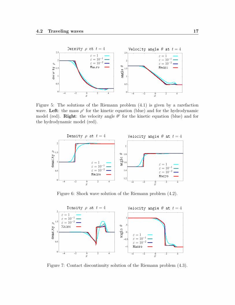
In figure 5, we represent the density ρε(x) and angle velocity θε(x) at t = 4 unittime. We do observe that, as ε → 0, the solution given by the kinetic equation(ρε, θε) gets closer and closer to the solution of the hydrodynamic model (ρ, u).The effect of ε can be seen as a “smoothing parameter”. It is consistent with thederivation of the hydrodynamic limit where the second order approximation in εgives a diffusion-type operator [17].

For our second simulation, we use a Riemann problem that generates a shocksolution. We use for that the initial condition:

(ρl, θl) = (1, 1.5) , (ρr, θr) = (2, 1.83). (4.2)

We plot the solutions of both the kinetic equation and hydrodynamic limit at timet = 4 unit time in figure 6. Once again, the moments (ρε, uε) do converge toward theshock profile given by the solution of the hydrodynamic model (ρ, u). We note thatthere is no analytic solution for the shock wave since the hydrodynamic model isnot conservative, we lack the Rankine-Hugoniot conditions to find an explicit valuefor the shock speed. Hence, it is quite remarkable that both the kinetic formulationand the hydrodynamic model give the same shock profile with the same speed.

An additional inspection of the solutions suggest that the solution of the kineticmodel might present cusp formation. For instance, in figure 5 (right), we observe a’blob’ forming at x ≈ 3.7 unit space, that vanishes as ε→ 0. There is a similar but’more disperse’ pattern in the figure 6 at x ≈ 1 unit space. The formation of cuspswill have a strong importance for the understanding of the kinetic model.

For our third simulation, the Riemann problem used is a contact discontinuity(see figure 7):

(ρl, θl) = (1, 1) , (ρr, θr) = (1,−1). (4.3)

Here, the solution of the hydrodynamic model is more complex than a rarefactionwave or a shock wave. As for the shock profile (figure 6), there is no analyticexpression for this solution. But once again, the solution given by the kineticequation does converge as ε → 0 toward the complex profile of the hydrodynamicmodel. Thus, these numerical simulations at the kinetic level confirm the relevanceof the profile observed at the macroscopic level.

4.2 Traveling waves 17

0

0.5

1

1.5

2

2.5

−4 −2 0 2 4

d

e

n

s

i

t

y

ρ

x

Density ρ at t = 4

ε = 1ε = 10−1

ε = 10−2

Ma ro

0

0.5

1

1.5

2

2.5

−4 −2 0 2 4

a

n

g

l

e

θ

x

Velo ity angle θ at t = 4

ε = 1ε = 10−1

ε = 10−2

Ma ro

Figure 5: The solutions of the Riemann problem (4.1) is given by a rarefactionwave. Left: the mass ρε for the kinetic equation (blue) and for the hydrodynamicmodel (red). Right: the velocity angle θε for the kinetic equation (blue) and forthe hydrodynamic model (red).

0

0.5

1

1.5

2

−4 −2 0 2 4

d

e

n

s

i

t

y

ρ

x

Density ρ at t = 4

ε = 1ε = 10−1

ε = 10−2

Ma ro

1.2

1.4

1.6

1.8

2

−4 −2 0 2 4

a

n

g

l

e

θ

x

Velo ity angle θ at t = 4

ε = 1ε = 10−1

ε = 10−2

Ma ro

Figure 6: Shock wave solution of the Riemann problem (4.2).

0

0.5

1

1.5

2

−4 −2 0 2 4

d

e

n

s

i

t

y

ρ

x

Density ρ at t = 4

ε = 1ε = 10−1

ε = 10−2

Ma ro

−1

−0.5

0

.5

1

−4 −2 0 2 4

a

n

g

l

e

θ

x

Velo ity angle θ at t = 4

ε = 1ε = 10−1

ε = 10−2

Ma ro

Figure 7: Contact discontinuity solution of the Riemann problem (4.3).

4.3 Vortex formation 18

4.3 Vortex formationIn all the previous simulations, we have used Neumann boundary conditions inorder to reduce the influence of the boundary of the domain on the dynamics. Wewould like now to investigate in more details the impact of boundary conditionson the dynamics. For this purpose, we compare the kinetic model (2.4) and themicroscopic model (2.1) in a bounded domain Ω with reflexive boundary conditions.At the microscopic level, each time a particle i hits the boundary (i.e. xi ∈ ∂Ω), itsvelocity ωi is reflected:

ωi = S∂Ω(x)(ωi) = ωi − 2〈ωi, η〉η

where η is the unit normal vector at ∂Ω(x) (see figure 8). Similarly, at the kineticlevel, reflexive boundary conditions impose that f satisfies at the boundary:

f(x, ω) = f(x, S∂Ω(x)(ω)) for x ∈ ∂Ω.

In other words, we have no-flux boundary conditions. In contrast to the kineticmodel, reflexive boundary conditions would be more delicate to implement for thehydrodynamic model due to the constraint |u| = 1. Moreover, the validity ofthe hydrodynamic model near the boundary is questionable due to the possibleformation of boundary layers (e.g. Prandtl’s boundary layer).

wall ∂Ω

ωi

S∂Ω(ωi)

xiη

ω

wall ∂Ω

x

f(x, S∂Ω(ω)) = f(x, ω)

S∂Ω(ω)

Figure 8: Left: Reflexive boundary conditions for the particle model. Once xireaches the boundary ∂Ω, its velocity ωi is reflected. Right: Reflexive boundaryconditions for the kinetic model: outgoing flux (i.e. f(x, ω)) equals the incomingflux (i.e. f(x, S∂Ω(ω))) at the boundary x ∈ ∂Ω in all direction ω.

Starting from a uniform distribution in space and velocity, we run the Vicsekmodel for both the particle and kinetic level. Both simulations are run on a squaredomain Ω of 10 space units. For the particle level, we perform three runs withrespectively 5 · 103, 104 and 5 · 104 particles with a radius of interaction R = .2and a time discretization of ∆t = .01 unit time. For the kinetic model, we use amesh grid ∆x = ∆y = .2 and a larger time discretization ∆t = .05 to reduce thenumerical viscosity. We use 32 modes to discretize the velocity distribution.

4.3 Vortex formation 19

After a transient period, both simulations converge toward a stationary stateconsisting of a vortex-type formation. In figure 9, we represent the spatial densityρ and macroscopic velocity u defined as:

ρ(x) =∫ 2π

0f(x, θ) dθ, ρ(x)u(x) =

∫ 2π

0ω(θ)f(x, θ) dθ,

with ω(θ) = (cos θ, sin θ)T . As a result of the reflexive boundary conditions and thealignment interaction, the flow u tends to follow the boundary. Here, the flow uis turning clockwise but it is equally probable that it would turn counter-clockwisesince the initial distribution is uniform in space and velocity.

We notice that the particle model has more fluctuations compared to the kineticmodel as we could expect. For instance, the solution of the kinetic model is invariantunder rotation of angle π/2 which is not the case in the particle model due tofluctuations. To measure the agreement and the discrepancy between the two spatialdistributions, we introduce the distribution ϕ(`) measuring the average density onthe squares C` centered at the origin with radius `:

C` = (x, y) ∈ R2 | max(|x|, |y|) = `.

In other words, ϕ(`) is defined for ` > 0 as:

ϕ(`) = 1|C`|

∫C`

ρ ds = 14`

∫‖(x,y)‖∞=`

ρ ds. (4.4)

We average over squares instead of circles to take into account the geometry ofthe domain Ω. As we observe in figure 10, the distributions ϕ(`) for the particleand kinetic models agree very well with each other. We observe some discrepancynear ` ≈ 0 and ` ≈ 5 corresponding respectively to the center and the boundary ofthe domain Ω. As we increase the number of particles, the discrepancies tend todisappear.

Overall, the kinetic model provides a reliable description of the microscopicmodel without the fluctuations. Moreover, the computation time of the micro-scopic model would drastically increase as the number of particles n becomes larger.Whereas, for the kinetic model, the computation time remains exactly the samewhen we increase the density.

Additional numerical investigations are required to better understand the dis-crepancy between the two curves. Both curves should coincide as the number ofparticles n and the number of modes N are approaching infinity since both methodsconverge to the analytic kinetic solution.

A way to obtain a quantification of such error will be analyzed in future work.As the number of particles n increases, one could estimate the convergence of theparticle model (2.1) by means of Wasserstein metrics [8,9]. Moreover, we anticipate

5 Conclusion 20

that the convergence analysis of our spectral method with respect to the numberof spectral modes N can be performed by adapting existing work on conservativespectral schemes [1,21]. Thus, one could estimate the relation between the numberof particles n and spectral modes N for the kinetic equation by measuring the orderof accuracy of both methods with respect to the analytic kinetic solution.

5 ConclusionWe presented the first numerical method for a kinetic description of the Vicsekswarming model, which poses a unique challenge as there is a distribution dependentcollision invariant to satisfy when computing the interaction term. The method useda spectral representation linked with a discrete constrained optimization to computethese interactions, and shows excellent agreement with the macroscopic equationswhen near that regime. The numerical results emphasize the importance of en-forcing the collision invariants in the system. Future work will seek to extend thisformulation to the three dimensional Vicsek equation, which has two GeneralizedCollisional Invariants instead of one. An important issue to be further developed isthe study of effects due to more intricate boundary conditions that can model moreadvanced wall avoidance, such as birds swerving when approaching a wall. Anotherinteresting application is using the kinetic equation to study the dynamics of thenon-conservative macroscopic equations that arise from this model, in particular,the formation of cusps. Finally, numerical analysis for the proposed scheme will bedeveloped. As mentioned earlier, we anticipate that the semi discrete error and con-vergence analysis as the number of spectral modes N grows large, as applied by [1]to the conservative spectral schemes for classical Boltzmann dynamics for binaryinteractions [21], may also work for the proposed approximation of orientationalinteractions in the present work.

5 Conclusion 21

−5

−3

−1

1

3

5

−5 −3 −1 1 3 5

y

x

P a r t i l e m o d e l

−5

−3

−1

1

3

5

−5 −3 −1 1 3 50

2

4

6

8

10

12

14

y

x

K i n e t i m o d e l

Figure 9: Left: density ρ and velocity u for the particle model (104 particles) att = 200 unit time on a square domain with reflexive boundary conditions. Right:ρ and u for the kinetic model in for the same condition. Both solutions are close toa vortex-formation.

1 2 3 4 5

2

4

6

8

radius `

averagedensity

ϕ(`)

Micro: (n = 5·103)Micro: (n = 1·104)Micro: (n = 5·104)Kinetic

Figure 10: The average density ϕ(`) (4.4) on the square C` for the particle model(dashed lines) and kinetic model (red) at time t = 200 (see figure 9). The distribu-tions agree well with each other with some discrepancy at the origin (` ≈ 0) andnear the boundary of the domain (` ≈ 5). The discrepancies reduce as the numberof particles increases.

REFERENCES 22

References[1] R.J. Alonso, I. Gamba, and S.H. Tharkabhushanam. Convergence and error es-

timates of the Lagrangian based Conservative Spectral method for BoltzmannEquation. Preprint, 2014.

[2] I. Aoki. A simulation study on the schooling mechanism in fish. Bulletin ofthe Japanese Society of Scientific Fisheries (Japan), 1982.

[3] M. Ballerini, N. Cabibbo, R. Candelier, A. Cavagna, E. Cisbani, I. Giardina,V. Lecomte, A. Orlandi, G. Parisi, and A. Procaccini. Interaction ruling an-imal collective behavior depends on topological rather than metric distance:Evidence from a field study. Proceedings of the National Academy of Sciences,105(4):1232, 2008.

[4] G. A Bird. Molecular gas dynamics and the direct simulation of gas flows.Clarendon Press, 1994.

[5] A. V. Bobylev. The theory of the nonlinear spatially un1form Boltzmannequat1on for Maxwell molecules. Mathematical physics reviews, 7:111, 1988.

[6] A. V. Bobylev and S. Rjasanow. Difference scheme for the Boltzmann equationbased on fast Fourier transform. European Journal of Mechanics-B/Fluids,16(2):293–306, 1997.

[7] A. V. Bobylev and S. Rjasanow. Fast deterministic method of solving the Boltz-mann equation for hard spheres. European Journal of Mechanics-B/Fluids,18(5):869–887, 1999.

[8] F. Bolley, J. A. Cañizo, and J. A. Carrillo. Mean-field limit for the stochasticVicsek model. Applied Mathematics Letters, 25(3):339–343, 2012.

[9] M. Bostan and J. A. Carrillo. Asymptotic fixed-speed reduced dynamics forkinetic equations in swarming. Mathematical Models and Methods in AppliedSciences, 23(13):2353–2393, 2013.

[10] J. Broadwell. Study of rarefied shear flow by the discrete velocity method. J.Fluid Mech, 19(3):401–414, 1964.

[11] C. Buet. A discrete-velocity scheme for the Boltzmann operator of rarefied gasdynamics. Transport Theory and Statistical Physics, 25(1):33–60, 1996.

[12] J. A. Cañizo, J. Carrillo, and J. Rosado. A well-posedness theory in measuresfor some kinetic models of collective motion. Mathematical Models and Methodsin Applied Sciences, 21(03):515–539, 2011.

REFERENCES 23

[13] Y. Chuang, M. R D’Orsogna, D. Marthaler, A. L Bertozzi, and L. S Chayes.State transitions and the continuum limit for a 2d interacting, self-propelledparticle system. Physica D: Nonlinear Phenomena, 232(1):33–47, 2007.

[14] I. D Couzin, J. Krause, R. James, G. D Ruxton, and N. R Franks. CollectiveMemory and Spatial Sorting in Animal Groups. Journal of Theoretical Biology,218(1):1–11, 2002.

[15] P. Degond, J. G. Liu, S. Motsch, and V. Panferov. Hydrodynamic models ofself-organized dynamics: derivation and existence theory. Methods and Appli-cations of Analysis, 20(2):89–114, 2013.

[16] P. Degond and S. Motsch. Continuum limit of self-driven particles with ori-entation interaction. Mathematical Models and Methods in Applied Sciences,18(1):1193–1215, 2008.

[17] P. Degond and T. Yang. Diffusion in a continuum model of self-propelledparticles with alignment interaction. Mathematical Models and Methods inApplied Sciences, 20(supp01):1459–1490, 2010.

[18] G. Dimarco and L. Pareschi. Numerical methods for kinetic equations. ActaNumerica, 23:369–520, 2014.

[19] F. Filbet and C. Mouhot. Analysis of spectral methods for the homogeneousBoltzmann equation. Transactions of the American Mathematical Society,363(4):1947–1980, 2011.

[20] F. Filbet and L. Pareschi. A numerical method for the accurate solution ofthe Fokker-Planck-Landau equation in the nonhomogeneous case. Journal ofComputational Physics, 179(1):1–26, 2002.

[21] I. Gamba and S. H. Tharkabhushanam. Spectral-Lagrangian methods for col-lisional models of non-equilibrium statistical states. Journal of ComputationalPhysics, 228(6):2012–2036, 2009.

[22] I. Gamba and S. H. Tharkabhushanam. Shock and boundary structure forma-tion by spectral-Lagrangian methods for the inhomogeneous Boltzmann trans-port equation. J. Comput. Math, 28(4):430–460, 2010.

[23] I. M. Gamba and J. R. Haack. A conservative spectral method for the Boltz-mann equation with anisotropic scattering and the grazing collisions limit.Journal of Computational Physics, 270:40–57, 2014.

REFERENCES 24

[24] Irene M. Gamba and Moon-Jin Kang. Global weak solutions for Kolmogorov-Vicsek type equations with orientational interaction. arXiv preprintarXiv:1502.00293, 2015.

[25] D. Goldstein, B. Sturtevant, and J. E. Broadwell. Investigations of the motionof discrete-velocity gases. Progress in Astronautics and Aeronautics, 117:100–117, 1989.

[26] S. Y Ha and E. Tadmor. From particle to kinetic and hydrodynamic descrip-tions of flocking. Kinetic and Related Models, 1(3):415–435, 2008.

[27] T. Inamuro and B. Sturtevant. Numerical study of discrete-velocity gases.Physics of Fluids A: Fluid Dynamics (1989-1993), 2(12):2196–2203, 1990.

[28] R. J LeVeque. Numerical Methods for Conservation Laws. Birkhäuser, 1992.

[29] A. Mogilner and L. Edelstein-Keshet. A non-local model for a swarm. Journalof Mathematical Biology, 38(6):534–570, 1999.

[30] A. B. Morris, P. L. Varghese, and D. B. Goldstein. Monte Carlo solution of theBoltzmann equation via a discrete velocity model. Journal of ComputationalPhysics, 230(4):1265–1280, 2011.

[31] S. Motsch and L. Navoret. Numerical simulations of a non-conservative hyper-bolic system with geometric constraints describing swarming behavior. Multi-scale Modeling Simulation, 9(3):1253–1275, 2011.

[32] L. Pareschi and B. Perthame. A Fourier spectral method for homogeneousBoltzmann equations. Transport Theory and Statistical Physics, 25(3-5):369–382, 1996.

[33] L. Pareschi and G. Russo. Numerical solution of the Boltzmann equation I:Spectrally accurate approximation of the collision operator. SIAM journal onnumerical analysis, 37(4):1217–1245, 2000.

[34] L. Pareschi, G. Russo, and G. Toscani. Fast spectral methods for theFokker-Planck-Landau collision operator. Journal of Computational Physics,165(1):216–236, 2000.

[35] J. K Parrish, S. V Viscido, and D. Grunbaum. Self-organized fish schools:an examination of emergent properties. Biological Bulletin, Marine BiologicalLaboratory, Woods Hole, 202(3):296–305, 2002.

[36] C. W Reynolds. Flocks, herds and schools: A distributed behavioral model. InACM SIGGRAPH Computer Graphics, volume 21, pages 25–34, 1987.

REFERENCES 25

[37] F. Rogier and J. Schneider. A direct method for solving the Boltzmann equa-tion. Transport Theory and Statistical Physics, 23(1-3):313–338, 1994.

[38] J. Toner and Y. Tu. Flocks, herds, and schools: A quantitative theory offlocking. Physical Review E, 58(4):4828–4858, 1998.

[39] C. M Topaz, A. L Bertozzi, and M. A Lewis. A Nonlocal Continuum Modelfor Biological Aggregation. Bulletin of Mathematical Biology, 68(7):1601–1623,2006.

[40] T. Vicsek, A. Czirók, E. Ben-Jacob, I. Cohen, and O. Shochet. Novel type ofphase transition in a system of self-driven particles. Physical Review Letters,75(6):1226–1229, 1995.

A Summary of the numerical scheme 26

A Summary of the numerical schemeWe summarize the different steps of the numerical scheme. We use the followingnotations: xi = i∆x, yi = j∆y, θs = s∆θ.

After the initialization of the distribution fi,j,s = f(xi, yj, θs), the numericalscheme consists in iterating the following splitting method.

1) Collisional operator: in each cell (xi, yj)

– Decomposition: compute the mean direction θ and deduce ckk

ck =∑s

f(θs+θ)P−k(θs)∆θ

M(θs). (A.1)

– Update: c∗k = ck + ∆tΛQ(ck).– Reconstruct f : fs = ∑

k c∗kPk(θs − θ).

2) Transport operator : for each velocity angle θs and in each case i, j

fi,j,s = fi,j,s −∆t cos θs

∆x (fi+ 12 ,j,s− fi− 1

2 ,j,s)− ∆t sin θs

∆y (fi,j+ 12 ,s− fi,j− 1

2 ,s),

where the indices i± 12 are computed using an upwind-method. For instance,

i+ 12 =

i+ 1 if cos(θs) ≤ 0i if cos(θs) > 0

Remark A.1 To estimate the coefficients ckk in (A.1), we need to perform achange of coordinates which creates error if θ is not a meshgrid point. To avoidthose interpolations approximations, we use a change of coordinates in the formula(A.1)

ck =∑s

f(θs)P−k(θs−θ)∆θ

M(θs−θ). (A.2)

Since Pn and M are explicit functions (3.4) (3.13), there is no additional cost inusing (A.2).

B Stability for the homogeneous equation 27

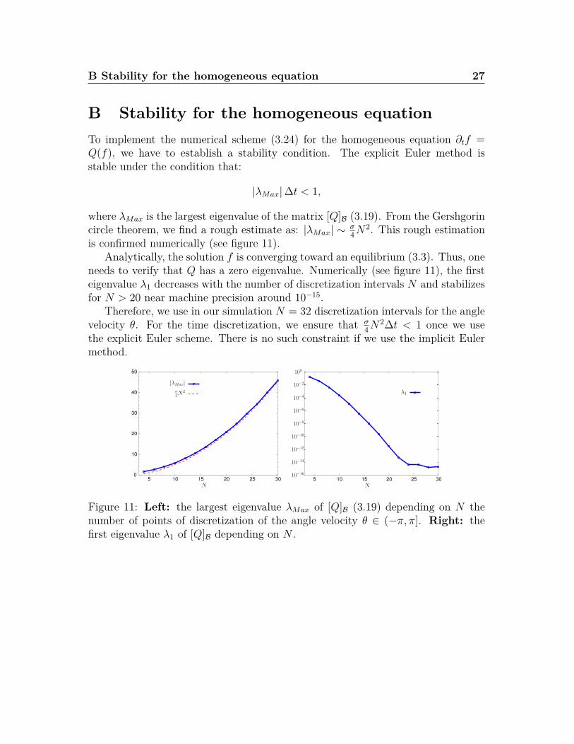
B Stability for the homogeneous equationTo implement the numerical scheme (3.24) for the homogeneous equation ∂tf =Q(f), we have to establish a stability condition. The explicit Euler method isstable under the condition that:

|λMax|∆t < 1,

where λMax is the largest eigenvalue of the matrix [Q]B (3.19). From the Gershgorincircle theorem, we find a rough estimate as: |λMax| ∼ σ

4N2. This rough estimation

is confirmed numerically (see figure 11).Analytically, the solution f is converging toward an equilibrium (3.3). Thus, one

needs to verify that Q has a zero eigenvalue. Numerically (see figure 11), the firsteigenvalue λ1 decreases with the number of discretization intervals N and stabilizesfor N > 20 near machine precision around 10−15.

Therefore, we use in our simulation N = 32 discretization intervals for the anglevelocity θ. For the time discretization, we ensure that σ

4N2∆t < 1 once we use

the explicit Euler scheme. There is no such constraint if we use the implicit Eulermethod.

0

10

20

30

40

50

5 10 15 20 25 30

N

|λMax|σ4N

2

5 10 15 20 25 3010−16

10−14

10−12

10−10

10−8

10−6

10−4

10−2

100

N

λ1

Figure 11: Left: the largest eigenvalue λMax of [Q]B (3.19) depending on N thenumber of points of discretization of the angle velocity θ ∈ (−π, π]. Right: thefirst eigenvalue λ1 of [Q]B depending on N .

C Accuracy of the numerical scheme (homogeneous case) 28

C Accuracy of the numerical scheme (homoge-neous case)

To measure the accuracy of the scheme, we take advantage that the solution of thehomogeneous equation has to converge to equilibrium (a Von Mises distributionM (3.3)). In figure 12, we measure the distance between the solution f(t, θ) ofthe homogeneous equation and the corresponding equilibrium (i.e. ‖f(t, .)−M‖H)at different times (T = 10, 20, 50) and for different number of modes N . Weobserve that at large time T = 50 (red curve), the distance is decaying exponentiallyfast with the number of modes. The distances reaches eventually 10−14 due tomachine precision error. This result is consistent with the accuracy of spectralmethods [1,19,33]. At time T = 10 and 20, the solution f(t, .) has not yet reacheda stationary state. Thus, even though we increase the number of modes N , thedistance does not decrease to zero.

20 40 60 80 100 120

10−15

10−12

10−9

10−6

10−3

number of modes N

‖f−

M‖ H

time T =10time T =20time T =50

Figure 12: Distance between the homogeneous solution f(t, θ) and the Von MisesdistributionM (3.3). At time T = 50 (red curve), the distance is decaying exponen-tially fast with the number of modes (N). Parameters for the simulation: σ = .2,∆t = .1.