The Astrophysical Journal, 786:59 (13pp), 2014 May 1 doi:10.1088/0004-637X/786/1/59C© 2014. The American Astronomical Society. All rights reserved. Printed in the U.S.A.

SPECTRAL ENERGY DISTRIBUTION FITTING OF HETDEX PILOT SURVEYLyα EMITTERS IN COSMOS AND GOODS-N

Alex Hagen1,7, Robin Ciardullo1,7, Caryl Gronwall1,7, Viviana Acquaviva2,Joanna Bridge1,7, Gregory R. Zeimann1,7, Guillermo A. Blanc3, Nicholas A. Bond4, Steven L. Finkelstein5,

Mimi Song5, Eric Gawiser6, Derek B. Fox1,7, Henry Gebhardt1,7, A. I. Malz1,7,Donald P. Schneider1,7, Niv Drory5, Karl Gebhardt5, and Gary J. Hill5

1 Department of Astronomy & Astrophysics, The Pennsylvania State University, 525 Davey Lab, University Park, PA 16802, USA;hagen@psu.edu, rbc@astro.psu.edu, caryl@astro.psu.edu, jsbridge@psu.edu, grzeimann@psu.edu,

dfox@astro.psu.edu, gebhardt@psu.edu, malz@psu.edu, dps@astro.psu.edu2 Department of Physics, New York City College of Technology, City University of New York,

300 Jay Street, Brooklyn, NY 11201, USA; vacquaviva@citytech.cuny.edu3 Observatories of the Carnegie Institution for Science, Pasadena, CA 91101, USA; gblancm@obs.carnegiescience.edu4 Cosmology Laboratory, NASA Goddard Space Flight Center, Greenbelt, MD 20771, USA; nicholas.bond@nasa.gov

5 Department of Astronomy, The University of Texas at Austin, Austin, TX 78712, USA; stevenf@astro.as.utexas.edu, mmsong@astro.as.utexas.edu,drory@astro.as.utexas.edu, gebhardt@astro.as.utexas.edu, hill@astro.as.utexas.edu

6 Department of Physics and Astronomy, Rutgers, The State University of New Jersey, Piscataway, NJ 08854, USA; gawiser@physics.rutgers.eduReceived 2013 December 13; accepted 2014 March 18; published 2014 April 16

ABSTRACT

We use broadband photometry extending from the rest-frame UV to the near-IR to fit the individual spectralenergy distributions of 63 bright (L(Lyα) > 1043 erg s−1) Lyα emitting galaxies (LAEs) in the redshift range1.9 < z < 3.6. We find that these LAEs are quite heterogeneous, with stellar masses that span over three ordersof magnitude, from 7.5 < log M/M� < 10.5. Moreover, although most LAEs have small amounts of extinction,some high-mass objects have stellar reddenings as large as E(B − V ) ∼ 0.4. Interestingly, in dusty objects theoptical depths for Lyα and the UV continuum are always similar, indicating that Lyα photons are not undergoingmany scatters before escaping their galaxy. In contrast, the ratio of optical depths in low-reddening systems canvary widely, illustrating the diverse nature of the systems. Finally, we show that in the star-formation-rate–log-massdiagram, our LAEs fall above the “main-sequence” defined by z ∼ 3 continuum selected star-forming galaxies. Inthis respect, they are similar to submillimeter-selected galaxies, although most LAEs have much lower mass.

Key words: cosmology: observations – galaxies: evolution – galaxies: high-redshift – galaxies: starburst

Online-only material: color figures

1. INTRODUCTION

Patridge & Peebles (1967) originally predicted that the Lyαemission line could be a very useful probe of the high-redshiftuniverse, and, while it took many years to detect this feature(Cowie & Hu 1998; Hu et al. 1998), Lyα emitting galaxies(LAEs) are now routinely observable from z ∼ 0.2 (Deharvenget al. 2008; Cowie et al. 2010) to z > 7 (Hu et al. 2010; Ouchiet al. 2010; Lidman et al. 2012; Ono et al. 2012). However,while the detection of Lyα in the high-redshift universe isrelatively common, the physics of this emission is still not wellunderstood. Since Lyα is a resonance transition, it is likely thateach photon scatters many times off intervening neutral materialbefore escaping into intergalactic space. As a result, even a smallamount of dust should extinguish the line, and indeed, only∼25% of Lyman-break galaxies (LBGs) at z ∼ 2–3 have enoughLyα in emission to be classified as an LAE (Shapley et al. 2003).While it is possible for dusty galaxies to create an escape pathfor Lyα via supernova-blown bubbles and/or exotic geometry(e.g., Verhamme et al. 2012) most analyses suggest that theLAE population as a whole is made up of young, low-mass,low-metallicity systems, possessing relatively little interstellardust (e.g., Gawiser et al. 2007; Guaita et al. 2011).

To date, most Lyα emitters have been detected via deepnarrow-band imaging with 4 m and 8 m class telescopes (e.g.,

7 Also at Institute for Gravitation and the Cosmos, The Pennsylvania StateUniversity, University Park, PA 16802, USA.

Gronwall et al. 2007; Ouchi et al. 2008). These surveys generallyextend to low Lyα luminosities and sample a wide range of thehigh-redshift galaxy luminosity function. Unfortunately, in thecontinuum, LAEs are usually quite faint, which makes studyingtheir spectral energy distributions (SEDs) difficult. As a result,most of our knowledge about those physical properties whichare encoded in the objects’ SEDs—information such as stellarmass, extinction, and population age—has come from stackingtechniques (e.g., Gawiser et al. 2007; Guaita et al. 2011). Theseanalyses only yield estimates for a “typical” LAE and may besubject to serious systematic biases associated with the stackingtechniques (Vargas et al. 2014). Moreover, those few programsthat have sought to measure the SEDs of individual LAEs (e.g.,Finkelstein et al. 2009; Nilsson et al. 2011; Yuma et al. 2010;Nakajima et al. 2012; McLinden et al. 2014) have generally beenrestricted to very small numbers of objects. These efforts havebeen able to provide hints as to the range of properties exhibitedby the population, but have been unable to probe the statisticsof the entire LAE population. Thus, while we have some ideaabout the mass and dust content of “representative” LAEs, thedistribution of physical parameters for the entire populationremains poorly constrained.

Here, we investigate the stellar populations of luminousLyα emitters by analyzing the individual SEDs of 63 1.9 <z < 3.6 LAEs detected by the McDonald 2.7 m telescope’sHobby–Eberly Telescope Dark Energy Experiment (HETDEX)Pilot Survey. In Section 2, we summarize the HETDEX PilotSurvey (HPS) and describe the ancillary ground-based, Hubble

1

https://ntrs.nasa.gov/search.jsp?R=20140017651 2018-08-03T09:49:43+00:00Z

The Astrophysical Journal, 786:59 (13pp), 2014 May 1 Hagen et al.

Space Telescope (HST) and Spitzer photometry which is avail-able for analysis. In Section 3, we briefly describe the SED-fitting code GalMC (Acquaviva et al. 2011) and the underlyingassumptions used to derive stellar mass, extinction, and agefrom a set of broadband photometry which extends from therest-frame UV through to the near-IR. We also outline the pro-cedures used to measure the physical sizes of the LAEs in amanner that is insensitive to the effects of cosmological surfacebrightness dimming. In Section 4, we present our results andshow that the population of luminous z ∼ 3 LAEs is quite het-erogeneous, with sizes extending from 0.5 kpc � r � 4 kpc,stellar masses ranging from 7.5 < log M/M� < 10.5, and dif-ferential extinctions varying between 0.0 < E(B − V ) < 0.4.We illustrate several trends involving LAE physical parameters,including a positive correlation between reddening and stellarmass, a positive correlation between stellar mass and galacticage, and a positive correlation between galaxy size and Lyαluminosity. We also examine the possible evolution of physicalproperties with redshift and compare our LAEs to other z ∼ 3objects on the star-forming galaxy main sequence. We concludeby discussing the implications of our results for the underlyingphysical mechanisms of Lyα escape in high redshift galaxies.

For this paper we adopt a cosmology with H0 =70 km s−1 Mpc−1, ΩM = 0.3, and ΩΛ = 0.7 (PlanckCollaboration 2013; Hinshaw et al. 2013).

2. OUR SAMPLE

The LAEs chosen for study were discovered with theGeorge & Cynthia Mitchell Spectrograph (previously known asVIRUS-P; Hill et al. 2008) on the 2.7 m Harlan J. Smith Tele-scope during the HPS (Adams et al. 2011). This integral-fieldinstrument, which employs an array of 246 4.′′2 diameter fibers,covers ∼3 arcmin2 of sky at a time, and delivers 5 Å resolutionspectra between the wavelengths 3500 Å and 5800 Å. The HPSitself surveyed a total of 169 arcmin2 in the COSMOS (Scovilleet al. 2007), GOODS-N (Giavalisco et al. 2004), MUNICS-S2(Drory et al. 2001), and XMM-LSS (Pierre et al. 2004) fieldsand reached a limiting line flux of 6.7 × 10−17 erg cm−2 s−1 at5000 Å (for 50% of its pointings) and 1.0 × 10−16 erg cm−2 s−1

at 5000 Å (for 90% of the pointings). The final HPS catalog con-sists of coordinates, redshifts, R-band magnitudes, line fluxes,and equivalent widths for 397 emission-line selected galaxies.Ninty-nine of these sources are non X-ray emitting LAEs with1.9 < z < 3.8, rest-frame equivalent widths EW0 > 20 Å, andLyα luminosities between 2.6 × 1042 and 1.1 × 1044 erg s−1

(Adams et al. 2011; Blanc et al. 2011). A total of 74 of theseHPS LAEs lie in the GOODS-N and COSMOS fields, wheredeep HST data is available. The redshift range for this subsampleis 1.9 < z < 3.6.

The process of assigning an optical counterpart to each HPSemission-line detection was challenging. As pointed out byAdams et al. (2011), there is an order of magnitude mismatchbetween the spatial resolution obtained from the 4.′′2 diameterfibers of VIRUS-P, and that delivered by the broadband imagersof HST. Thus, each assignment was done in a Bayesian manner,by calculating the likelihood of association for each objectwithin a 10′′ window of the nominal position obtained fromthe spectroscopy (see Section 5.3 of Adams et al. 2011).Formally, the median probability for identifying the correctoptical counterpart was 64%. However, as discussed below in thefinal paragraph of Section 3.1, there is no statistical differencebetween the distribution of SED properties for a sample LAEs

with high-probability and/or confirmed counterparts and thatfor the sample of lower-probability associations.

In total, we identified 67 HPS LAEs with optical counterparts.Four of these objects (HPS IDs 144, 145, 160, and 196) wereremoved from our analysis based on the work of Blanc et al.(2011), who showed that their UV slopes were more consistentwith those of foreground [O ii] emitters than LAEs. This cullingleft us with 63 objects for analysis. Since the X-ray data inGOODS-N and COSMOS is deep enough to rule out most activegalactic nuclei, we believe that the bulk of these objects are trueLyα emitting sources with 1.9 < z < 3.6 and monochromaticLyα luminosities between 3.4 × 1042 and 3.8 × 1043 erg s−1.

Before proceeding further, we should note that the LAEsdiscovered by the HPS are significantly more luminous thanthe Lyα emitters found by most narrow-band surveys. Whilethe 2 < z < 3 observations of Gronwall et al. (2007), Ouchiet al. (2008), and Guaita et al. (2010) typically reach Lyα 90%completeness levels of L(Lyα) ∼ 1042 erg s−1, the median HPSlimit is five times brighter than this. On the other hand, sincethe Lyα luminosity limit of the HPS is very nearly constantacross the survey’s entire spectral range (see Figure 1 of Blancet al. 2011), the data set covers an order of magnitude moreco-moving volume than a typical narrow-band survey, withV = 5.63 × 105 Mpc3 in the COSMOS and GOODS-N regionsalone. This allows us to obtain good statistics on the bright endof the LAE population, and explore evolution over ∼1.6 Gyr ofcosmic time.

The HPS fields, and in particular, the COSMOS andGOODS-N regions are rich in deep, ancillary imaging and pro-vide up to 18 photometric data points for SED fitting. Tables 1and 2 summarize these data. Most of the HPS/COSMOS andHPS/GOODS-N fields are part of CANDELS (Grogin et al.2011; Koekemoer et al. 2011), and 49 out of our 63 LAEshave deep HST optical and near-IR photometry (Song et al.2014; Finkelstein et al. 2013) from this program. Moreover,all of our targets have photometry from Adams et al. (2011),who used the deep ground-based images of COSMOS as theirsource frames (Capak et al. 2007). Note that many of the LAEstargeted in this survey are too faint in the continuum to bepresent in the published COSMOS and GOODS photometriccatalogs; for these objects, AB magnitudes were determinedby re-measuring the original images using the positions of theHST optical counterparts. Still, there are some non-detections.When this occurred, an upper flux limit was assigned as the1σ uncertainty of the local sky value. In some cases, theselimits were crucial for constraining the SED properties of ourtargets.

Data at longer wavelengths come from observations with theSpitzer telescope. Once again, most LAEs are far too faint to bepresent in the S-COSMOS and GOODS-N Spitzer catalogs,as these analyses have relatively high detection thresholds(1 μJy in IRAC channel 1). Since the rest-frame near-IR isextremely important for determining stellar mass, we performedour own aperture photometry on these frames using MOPEX8

(Makovoz & Marleau 2005) at the known LAE positions.After experimenting with a variety of apertures, we settledon a photometric radius of 3.′′6, and then applied an aperturecorrection as described in the IRAC Instrument Handbook9.

8 Information on MOPEX is available athttp://irsa.ipac.caltech.edu/data/SPITZER/docs/dataanalysistools/tools/mopex/.9 http://irsa.ipac.caltech.edu/data/SPITZER/docs/irac/iracinstrumenthandbook/28/

2

The Astrophysical Journal, 786:59 (13pp), 2014 May 1 Hagen et al.

Table 1COSMOS Field Photometry

Telescope Instrument Filter Central λ Original Photometry 5σ Limits(Å) Survey (AB)

CFHT Megaprime u* 4065 COSMOS Adams et al. (2011) 26.5Subaru Suprime-Cam B 4788 COSMOS Adams et al. (2011) 27.4Subaru Suprime-Cam V 5730 COSMOS Adams et al. (2011) 27.2Subaru Suprime-Cam r+ 6600 COSMOS Adams et al. (2011) 26.9HST ACS F814W 7461 CANDELS Song et al. (2014) 27.5Subaru Suprime-Cam i+ 7850 COSMOS Adams et al. (2011) 26.9Subaru Suprime-Cam z+ 8700 COSMOS Adams et al. (2011) 25.6UKIRT WFCAM J 12850 COSMOS Adams et al. (2011) 23.6HST WFC3 F125W 13250 CANDELS Song et al. (2014) 26.4HST WFC3 F160W 14460 CANDELS Song et al. (2014) 26.5CFHT WIRCAM K 21400 COSMOS Adams et al. (2011) 23.6Spitzer IRAC Channel 1 37440 S-COSMOS This paper 23.9Spitzer IRAC Channel 2 44510 S-COSMOS This paper 23.3Spitzer IRAC Channel 3 59950 S-COSMOS This paper 21.3Spitzer IRAC Channel 4 84870 S-COSMOS This paper 21.0

Note. CANDELS covers 32 of 42 objects in this field.

Table 2GOODS-N Field Photometry

Telescope Instrument Filter Central λ Original Photometry 5σ Limits(Å) Survey (AB)

Mayall MOSAIC U 4065 GOODS Adams et al. (2011) 27.1HST ACS F435W 4570 CANDELS Finkelstein et al. (2013) 27.8Subaru Suprime-Cam B 4788 GOODS Adams et al. (2011) 26.9Subaru Suprime-Cam V 5730 GOODS Adams et al. (2011) 26.8Subaru Suprime-Cam r+ 6600 GOODS Adams et al. (2011) 26.6HST ACS F606W 6690 CANDELS Finkelstein et al. (2013) 27.6HST ACS F775W 7380 CANDELS Finkelstein et al. (2013) 27.5Subaru Suprime-Cam i+ 7850 GOODS Adams et al. (2011) 25.6HST ACS F850LP 8610 CANDELS Finkelstein et al. (2013) 27.3Subaru Suprime-Cam z+ 8700 GOODS Adams et al. (2011) 25.4HST WFC3 F105W 11783 CANDELS Finkelstein et al. (2013) 26.6HST WFC3 F125W 13250 CANDELS Finkelstein et al. (2013) 26.4HST WFC3 F160W 14460 CANDELS Finkelstein et al. (2013) 26.5UH 2.2 m QUIRC H + K ′ 20200 GOODS Adams et al. (2011) 22.1Spitzer IRAC Channel 1 37440 GOODS This paper 23.9Spitzer IRAC Channel 2 44510 GOODS This paper 23.3Spitzer IRAC Channel 3 59950 GOODS This paper 21.3Spitzer IRAC Channel 4 84870 GOODS This paper 21.0

Note. CANDELS covers 17 of 21 objects in this field.

3. DATA ANALYSIS

3.1. Spectral Energy Distribution Fitting

The SED of a galaxy encodes a number of physical param-eters, including stellar mass, age, dust content, and the currentstar formation rate (SFR). For example, since a galaxy’s near-IR flux arises principally from the evolved stars of all stellarpopulations, that part of the SED traces the system’s total stellarmass (Bell & de Jong 2001; Zibetti et al. 2009). In contrast,the slope of a galaxy’s far UV (∼1600 Å) continuum is fixedby the Rayleigh–Jeans tail of the blackbody emission from hot,young stars. The amplitude of the UV continuum thus yieldsthe SFR and any flattening of the UV continuum’s slope is mostlikely due to the effects of dust (Kennicutt 1998; Calzetti 2001).Estimates of population age come primarily from the regionsin between, as features such as the Balmer and 4000 Å breaksare sensitive to the main sequence turnoff and the exact mix ofintermediate age stars (e.g., Kauffmann et al. 2003).

To extract this information, we began with the populationsynthesis models of Bruzual & Charlot (2003), which wereupdated in 2007 (BC07) with an improved treatment of thethermal-pulsing asymptotic giant branch (TP-AGB) phase ofstellar evolution. This phase of stellar evolution can be impor-tant for systems older than ∼108 yr, which is ∼30% of oursample (see Section 4.4). We also performed fits using the olderBC03 models, but due to the generally young ages of the stellarpopulations, these fits were statistically indistinguishable fromthe 2007 models. For the remainder of this paper, we will onlyrefer to our BC07 results. For consistency with the works ofGuaita et al. (2011) and Acquaviva et al. (2011), we adopteda Salpeter (1955) initial mass function (IMF) over the range0.1 M� < M < 100 M�, a Calzetti (2001) extinction law,and a Madau (1995) model for the effects of intervening inter-galactic absorption. Since stellar metal abundances are poorlyconstrained by broadband SED measurements, we fixed themetallicity of our models to Z = 0.2 Z�; this is roughly the

3

The Astrophysical Journal, 786:59 (13pp), 2014 May 1 Hagen et al.

0

.5

1

1.5

2

0

5

10

15

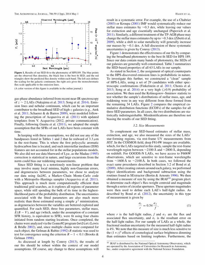
Figure 1. Results of our SED fit to the photometry of HPS189. The blue pointsare the observed flux densities, the black line is the best fit SED, and the redtriangles show the predicted flux density within each band. The left axis definesthe scaling for the galactic continuum; the right axis gives the monochromaticflux scale applicable to the emission lines.

(A color version of this figure is available in the online journal.)

gas-phase abundance inferred from recent near-IR spectroscopyof z ∼ 2 LAEs (Nakajima et al. 2013; Song et al. 2014). Emis-sion lines and nebular continuum, which can be an importantcontributor to the broadband SED of high-z galaxies (e.g., Ateket al. 2011; Schaerer & de Barros 2009), were modeled follow-ing the prescription of Acquaviva et al. (2011) with updatedtemplates from V. Acquaviva (2012, private communication).Finally, following Guaita et al. (2011), we adopted the simpleassumption that the SFRs of our LAEs have been constant withtime.

In keeping with these assumptions, we did not use any of thebandpasses listed in Tables 1 and 2 that lie redward of 3.3 μmin the rest-frame. This is where the first polycyclic aromatichydrocarbon line is located, and such interstellar medium (ISM)features are not accounted for in the stellar populations models.We also did not use data blueward of Lyα, as the Madau (1995)correction is statistical in nature, and large excursions from thenorm could bias our reddening measurements.

Since SED fitting is a notoriously non-linear problem thatmay involve many local minima, highly non-Gaussian errors,and degeneracies between parameters, we chose to analyzeour data using GalMC, a Markov-Chain Monte-Carlo codewith a Metropolis–Hastings sampler (Acquaviva et al. 2011).This approach is much more computationally efficient thantraditional grid searches, as it explores all regions of parameterspace, while still spending the bulk of its time in the highest-likelihood parts of the probability distribution. The uncertaintiesassociated with the fitted parameters are also much morerealistic than those estimated using a simple χ2 minimization,as degeneracies between the variables are bettered explored andquantified. For each SED, three free parameters, stellar mass,E(B − V ), and age (which, under the assumption of a constantSFR history, is equivalent to SFR), were fit using four chainsinitiated from random starting locations. Once completed, thechains were analyzed via theCosmoMC programGetDist (Lewis& Bridle 2002), and, since multiple chains were computed foreach object, the Gelman & Rubin (1992) R statistic was used totest for convergence using the criterion R − 1 < 0.1 (Brooks &Gelman 1998).

As discussed at length by Conroy (2013), the results ofour fits should be robust within the context of our modelassumptions. Of course, any change to these assumptions will

result in a systematic error. For example, the use of a Chabrier(2003) or Kroupa (2001) IMF would systematically reduce ourstellar mass estimates by ∼0.3 dex, while leaving our valuesfor extinction and age essentially unchanged (Papovich et al.2011). Similarly, a different treatment of the TP-AGB phase maychange the stellar mass estimates by up to ∼0.3 dex (Zibetti et al.2009), while a shift to solar metallicity will generally increaseour masses by ∼0.1 dex. A full discussion of these systematicuncertainties is given by Conroy (2013).

Figure 1 demonstrates the effectiveness of our fits by compar-ing the broadband photometry to the best fit SED for HPS 189.Since our data contain many bands of photometry, the SEDs ofour galaxies are generally well constrained. Table 3 summarizesthe SED-based properties of all 63 LAEs in our sample.

As stated in Section 2, the assignment of optical counterpartsto the HPS-discovered emission lines is probabilistic in nature.To investigate this further, we constructed a “clean” sampleof HPS-LAEs, using a set of 29 candidates with either spec-troscopic confirmations (Finkelstein et al. 2011; Chonis et al.2013; Song et al. 2014) or a very high (�0.9) probability ofassociation. We then used the Kolmogorov–Smirnov statistic totest whether the sample’s distributions of stellar mass, age, andreddening were in any way different from those formed fromthe remaining 34 LAEs. Figure 2 compares the empirical cu-mulative distribution functions (ECDFs) of the samples for allthree SED parameters. In all cases, the two distributions are sta-tistically indistinguishable. Misidentifications are therefore notbiasing the results of our SED fitting.

3.2. Size Measurements

To complement our SED-based estimates of stellar mass,extinction, and age, we also measured the sizes of the LAEs’star-forming regions, via rest-frame UV measurements fromHST. In the COSMOS field, deep F814W images are available,which, for the LAEs targeted in this study, sample the rest-framewavelength region between ∼2100 Å and ∼2800 Å, dependingon redshift. For GOODS-N LAEs, we have access to F606Wobservations, which are sensitive to rest-frame wavelengthsfrom ∼1600 Å to ∼2100 Å. In both cases, we followed theexact same procedures described in Section 3.2 of Bond et al.(2009). After creating cutouts around each galaxy, we performedobject identifications and background subtraction using theroutines found in SExtractor (Bertin & Arnouts 1996). We thenobtained a measure of size by using the IRAF10 program photto determine each object’s flux-weight centroid and magnitudethrough a series of circular apertures. These aperture magnitudeswere then used to define each LAE’s half-light radius. Asdescribed by Bond et al. (2012), the uncertainty in this typeof measurement is given by

σr

r= 0.54

σf

f, (1)

where r is the half-light radius, f and σf are the flux andassociated flux uncertainty, and σr is the resultant error onthe half-light radius. For our sample of LAEs as a whole, thefractional median uncertainty for the measured half-light radiusis 4%. We note that this measure of size is much less sensitive tothe (1 + z)4 effects of cosmological surface brightness dimmingthan estimates based on limiting isophotes. Furthermore, the

10 IRAF is distributed by the National Optical Astronomy Observatory, whichare operated by the Association of Universities for Research in Astronomy,Inc., under cooperative agreement with the National Science Foundation.

4

The Astrophysical Journal, 786:59 (13pp), 2014 May 1 Hagen et al.

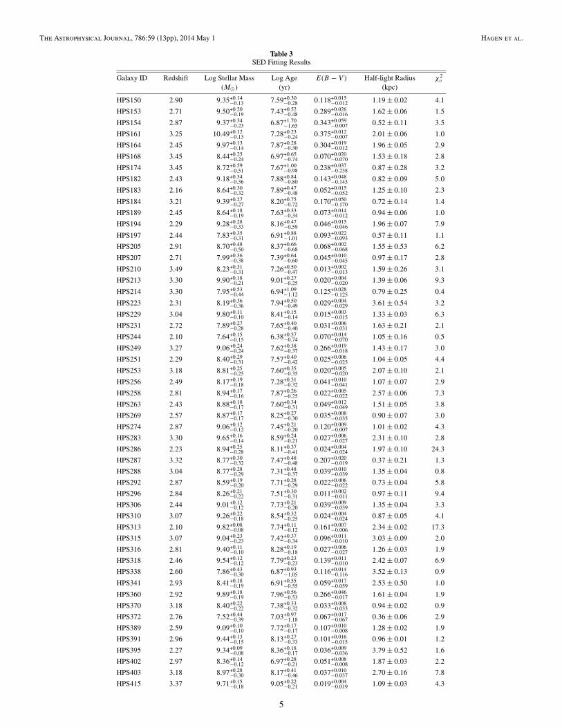
Table 3SED Fitting Results

Galaxy ID Redshift Log Stellar Mass Log Age E(B − V ) Half-light Radius χ2ν

(M�) (yr) (kpc)

HPS150 2.90 9.35+0.14−0.13 7.59+0.30

−0.28 0.118+0.015−0.012 1.19 ± 0.02 4.1

HPS153 2.71 9.50+0.20−0.19 7.43+0.52

−0.48 0.289+0.026−0.016 1.62 ± 0.06 1.5

HPS154 2.87 9.37+0.34−0.23 6.87+1.70

−1.65 0.343+0.059−0.007 0.52 ± 0.11 3.5

HPS161 3.25 10.49+0.12−0.13 7.28+0.23

−0.24 0.375+0.012−0.007 2.01 ± 0.06 1.0

HPS164 2.45 9.97+0.13−0.14 7.87+0.28

−0.30 0.304+0.019−0.012 1.96 ± 0.05 2.9

HPS168 3.45 8.44+0.25−0.24 6.97+0.65

−0.74 0.070+0.020−0.070 1.53 ± 0.18 2.8

HPS174 3.45 8.72+0.59−0.51 7.67+1.00

−0.98 0.238+0.037−0.238 0.87 ± 0.28 3.2

HPS182 2.43 9.18+0.34−0.36 7.88+0.84

−0.80 0.143+0.048−0.143 0.82 ± 0.09 5.0

HPS183 2.16 8.64+0.30−0.32 7.89+0.47

−0.48 0.052+0.015−0.052 1.25 ± 0.10 2.3

HPS184 3.21 9.39+0.27−0.27 8.20+0.75

−0.72 0.170+0.050−0.170 0.72 ± 0.14 1.4

HPS189 2.45 8.64+0.18−0.19 7.63+0.33

−0.34 0.073+0.014−0.012 0.94 ± 0.06 1.0

HPS194 2.29 9.28+0.28−0.33 8.16+0.47

−0.59 0.046+0.015−0.046 1.96 ± 0.07 7.9

HPS197 2.44 7.83+0.35−0.31 6.91+0.88

−1.01 0.093+0.022−0.093 0.57 ± 0.11 1.1

HPS205 2.91 8.70+0.48−0.50 8.37+0.66

−0.68 0.068+0.002−0.068 1.55 ± 0.53 6.2

HPS207 2.71 7.99+0.36−0.38 7.39+0.64

−0.60 0.045+0.010−0.045 0.97 ± 0.17 2.8

HPS210 3.49 8.23+0.31−0.31 7.26+0.50

−0.47 0.013+0.002−0.013 1.59 ± 0.26 3.1

HPS213 3.30 9.90+0.18−0.21 9.01+0.27

−0.25 0.020+0.004−0.020 1.39 ± 0.06 9.3

HPS214 3.30 7.95+0.53−0.44 6.94+1.09

−1.12 0.125+0.028−0.125 0.79 ± 0.25 0.4

HPS223 2.31 8.19+0.36−0.36 7.94+0.50

−0.49 0.029+0.004−0.029 3.61 ± 0.54 3.2

HPS229 3.04 9.80+0.11−0.10 8.41+0.15

−0.14 0.015+0.003−0.015 1.33 ± 0.03 6.3

HPS231 2.72 7.89+0.27−0.28 7.65+0.40

−0.40 0.031+0.006−0.031 1.63 ± 0.21 2.1

HPS244 2.10 7.64+0.15−0.15 6.38+0.57

−0.74 0.070+0.014−0.070 1.05 ± 0.16 0.5

HPS249 3.27 9.06+0.24−0.24 7.62+0.38

−0.37 0.266+0.019−0.018 1.43 ± 0.17 3.0

HPS251 2.29 8.40+0.29−0.31 7.57+0.40

−0.42 0.025+0.006−0.025 1.04 ± 0.05 4.4

HPS253 3.18 8.81+0.25−0.25 7.60+0.35

−0.35 0.020+0.005−0.020 2.07 ± 0.10 2.1

HPS256 2.49 8.17+0.19−0.18 7.28+0.31

−0.32 0.041+0.010−0.041 1.07 ± 0.07 2.9

HPS258 2.81 8.94+0.17−0.16 7.87+0.26

−0.25 0.022+0.005−0.022 2.57 ± 0.06 7.3

HPS263 2.43 8.88+0.18−0.17 7.60+0.34

−0.31 0.049+0.012−0.049 1.51 ± 0.05 3.8

HPS269 2.57 8.87+0.17−0.17 8.25+0.27

−0.30 0.035+0.008−0.035 0.90 ± 0.07 3.0

HPS274 2.87 9.06+0.12−0.12 7.45+0.21

−0.20 0.120+0.009−0.007 1.01 ± 0.02 4.3

HPS283 3.30 9.65+0.16−0.14 8.59+0.24

−0.21 0.027+0.006−0.027 2.31 ± 0.10 2.8

HPS286 2.23 8.94+0.25−0.28 8.11+0.37

−0.41 0.024+0.004−0.024 1.97 ± 0.10 24.3

HPS287 3.32 8.77+0.30−0.32 7.47+0.48

−0.48 0.207+0.020−0.019 0.37 ± 0.21 1.3

HPS288 3.04 8.77+0.28−0.29 7.31+0.48

−0.37 0.039+0.010−0.039 1.35 ± 0.04 0.8

HPS292 2.87 8.59+0.19−0.20 7.71+0.28

−0.29 0.022+0.006−0.022 0.73 ± 0.04 5.8

HPS296 2.84 8.26+0.21−0.22 7.51+0.30

−0.31 0.011+0.002−0.011 0.97 ± 0.11 9.4

HPS306 2.44 9.01+0.12−0.12 7.73+0.21

−0.20 0.039+0.009−0.039 1.35 ± 0.04 3.3

HPS310 3.07 9.26+0.22−0.18 8.54+0.32

−0.25 0.024+0.004−0.024 0.87 ± 0.05 4.1

HPS313 2.10 9.82+0.08−0.08 7.74+0.11

−0.12 0.161+0.007−0.006 2.34 ± 0.02 17.3

HPS315 3.07 9.04+0.23−0.23 7.42+0.37

−0.34 0.096+0.011−0.010 3.03 ± 0.09 2.0

HPS316 2.81 9.40+0.11−0.10 8.28+0.19

−0.18 0.027+0.006−0.027 1.26 ± 0.03 1.9

HPS318 2.46 9.54+0.12−0.12 7.79+0.23

−0.23 0.139+0.011−0.010 2.42 ± 0.07 6.9

HPS338 2.60 7.86+0.43−0.30 6.87+0.93

−1.05 0.116+0.014−0.116 3.52 ± 0.13 0.9

HPS341 2.93 8.41+0.18−0.19 6.91+0.55

−0.55 0.059+0.017−0.059 2.53 ± 0.50 1.0

HPS360 2.92 9.89+0.18−0.19 7.96+0.56

−0.53 0.266+0.046−0.017 1.61 ± 0.04 1.9

HPS370 3.18 8.40+0.22−0.22 7.38+0.33

−0.32 0.033+0.008−0.033 0.94 ± 0.02 0.9

HPS372 2.76 7.52+0.44−0.39 7.03+0.97

−1.18 0.067+0.017−0.067 0.36 ± 0.06 2.9

HPS389 2.59 9.09+0.10−0.10 7.72+0.17

−0.17 0.107+0.010−0.008 1.28 ± 0.02 1.9

HPS391 2.96 9.44+0.13−0.15 8.13+0.27

−0.33 0.101+0.016−0.015 0.96 ± 0.01 1.2

HPS395 2.27 9.34+0.09−0.08 8.36+0.18

−0.17 0.036+0.009−0.036 3.79 ± 0.52 1.6

HPS402 2.97 8.36+0.14−0.12 6.97+0.28

−0.21 0.051+0.008−0.008 1.87 ± 0.03 2.2

HPS403 3.18 8.97+0.28−0.30 8.17+0.41

−0.46 0.037+0.010−0.037 2.70 ± 0.16 7.8

HPS415 3.37 9.71+0.15−0.18 9.05+0.22

−0.21 0.019+0.004−0.019 1.09 ± 0.03 4.3

5

The Astrophysical Journal, 786:59 (13pp), 2014 May 1 Hagen et al.

Table 3(Continued)

Galaxy ID Redshift Log Stellar Mass Log Age E(B − V ) Half-light Radius χ2ν

(M�) (yr) (kpc)

HPS419 2.23 10.00+0.13−0.12 8.83+0.28

−0.25 0.132+0.019−0.014 1.67 ± 0.02 1.8

HPS420 2.93 8.67+0.18−0.18 7.71+0.28

−0.28 0.052+0.011−0.052 0.56 ± 0.01 5.4

HPS426 3.40 9.57+0.20−0.20 8.84+0.42

−0.30 0.049+0.011−0.049 0.70 ± 0.02 4.1

HPS428 3.34 9.46+0.10−0.11 8.04+0.18

−0.20 0.072+0.010−0.009 1.93 ± 0.07 2.9

HPS434 2.27 9.03+0.31−0.26 8.74+0.71

−0.56 0.073+0.026−0.073 1.03 ± 0.04 3.1

HPS436 2.42 8.36+0.15−0.16 7.23+0.24

−0.26 0.077+0.009−0.007 1.78 ± 0.02 1.5

HPS447 3.13 8.39+0.10−0.11 6.36+0.60

−0.74 0.033+0.009−0.033 3.60 ± 0.11 2.5

HPS462 2.21 10.48+0.13−0.11 8.61+0.32

−0.29 0.296+0.024−0.020 1.38 ± 0.84 2.8

HPS466 3.24 9.04+0.03−0.03 6.82+0.05

−0.04 0.134+0.004−0.004 1.51 ± 0.01 12.9

HPS474 2.27 8.97+0.20−0.20 7.95+0.35

−0.33 0.096+0.014−0.010 1.18 ± 0.02 8.3

observations differ in depth (COSMOS is a single orbit whileGOODS is 2.5 orbits), and so any biases from surface brightnesslimits can be found by comparing the half-light radii from bothsurveys. A two-sample K-S test showed that the distributionsof half-light radii derived from GOODS and COSMOS are notsignificantly different and thus we should not be concernedabout effects from cosmological surface brightness dimming.

4. RESULTS

Table 3 gives the best-fit solutions to our SED fits, theirreduced χ2 values, and the LAE’s half-light radii as measuredon the HST frames. We discuss these results below.

4.1. Size

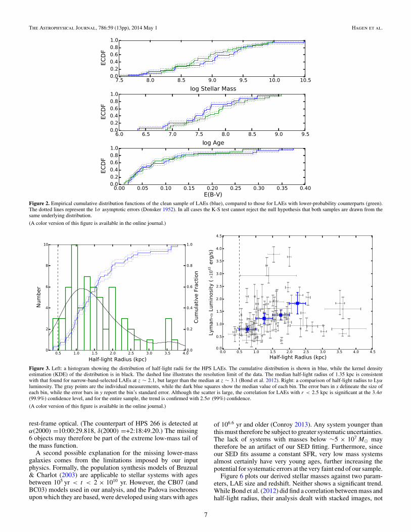
The left-hand panel of Figure 3 shows the distribution of half-light radii for the 63 luminous Lyα emitters in our sample.11

From the figure, it is clear that the highly luminous LAEs ofthe HPS have a wide range of sizes: while the peak of thedistribution is close to 1.2 kpc, there is a distinct tail that extendsall the way out to ∼4 kpc. The median of the distribution is1.35+0.08

−0.10 kpc, where the 68% confidence interval comes from abootstrap analysis (Efron 1987). For comparison, the typical sizeof the narrow-band selected 2 < z < 3 LAEs studied by Bondet al. (2012) is ∼1.0 kpc, while that for z ∼ 3 LBGs is closeto 4 kpc (Pentericci et al. 2010). As demonstrated by Spearmanrank correlation coefficient (ρ = −0.15) and Figure 4, thesesizes show no significant correlation with redshift; this resultis consistent with that of Malhotra et al. (2012), who also sawno size evolution in samples of narrow-band selected LAEsbetween 2.5 < z < 6. This is in contrast with the strongevolution seen in the sizes of LBGs over the same redshiftrange (e.g., Ferguson et al. 2004).

On the other hand, as the right-hand panel of Figure 3 shows,there is a relation between LAE half-light radius, as measured inthe rest-frame UV, and the amount of luminosity emitted in theLyα line. Although the scatter in the diagram is substantial, theSpearman rank order coefficient reveals a positive correlation

11 This type of plot will be used throughout this work and shows a histogram,a kernel density estimation (KDE), and the empirical cumulative distributionfunction (ECDF). All KDEs contained herein use a Gaussian kernel and werecalculated using the density function in R (R Core Team 2012). The bandwidthfor each KDE was found using the rule of thumb from Scott (1992). A simplechange in the choice of bins for a histogram can change the interpretation ofthe science; since KDEs do not require binning, they do not suffer from thiseffect. Every ECDF plotted will also have dotted upper and lower limits, whichrepresent the 1σ asymptotic errors (Donsker 1952).

between the two variables (ρ = +0.31), which is significantat the 2.5σ (99%) level. Moreover, up to a half-light radius of2.5 kpc, ρ = +0.45, implying a 3.4σ (99.9% confidence) result.Within this range, Lyα luminosity appears to grow linearly withgalaxy size with a slope of 0.6 ± 0.2 × 1043 erg s−1 kpc−1.Unfortunately, the data outside this range are too sparselypopulated to draw any conclusions.

4.2. Stellar Mass

At 2 < z < 3, SED stacking analyses have producedestimates for the median LAE mass in the range of ∼108 to1010 M�, depending on whether the samples under study weredetectable on Spitzer/IRAC images (Lai et al. 2008; Guaitaet al. 2011; Acquaviva et al. 2011). In the left-hand panel ofFigure 5, we show the distribution of individual LAE massesderived from our constant SFR model. Although the medianmass of log(M/M�) = 8.97+0.06

−0.17 lies in the range inferredfrom the previous stacking analyses, the data span a factor ofa thousand, from M ∼ 107.5 to 1010.5 M�. This distribution isconsistent with that recently found by McLinden et al. (2014)for a set of extremely luminous (L(Lyα) > 1043 erg s−1)z ∼ 3.1 LAEs found via narrow-band imaging. Interestinglyif we fit our LAE mass distribution with a power law over therange 8.5 < log M/M� < 10.5, then the most-likely slope,α = −1.3 ± 0.1, is similar, or perhaps only slightly shallowerthan the slope usually adopted for the epoch’s galaxy massfunction (e.g., Muzzin et al. 2013; Tomczak et al. 2013). Thissuggests that bright Lyα emitters are drawn from an underlyingdistribution that is not strongly dependent on stellar mass.Moreover, as the right-hand panel of Figure 5 demonstrates,there is no obvious correlation between stellar mass and Lyαluminosity: at any log L, one can find LAEs of all masses,and galaxies of any given mass can have a wide range of Lyαluminosity. Unless this behavior abruptly changes at low Lyαluminosity, it would appear that large-volume LAE surveys arean excellent way of sampling virtually the entire range of thehigh-redshift galaxy mass function.

One additional feature of Figure 5 worth noting is the absenceof LAEs with masses less than ∼5 × 107 M�. There are twopossible reasons for this. The first is the depth of the imaging:there are seven sources in the HPS survey for which Adamset al. (2011) could find no obvious counterpart in the rest-frameUV. An examination of the CANDELS frames and grism spectrafrom the 3D-HST program (van Dokkum et al. 2013) reveals thatonly one of these missing objects has any detectable flux in the

6

The Astrophysical Journal, 786:59 (13pp), 2014 May 1 Hagen et al.

Figure 2. Empirical cumulative distribution functions of the clean sample of LAEs (blue), compared to those for LAEs with lower-probability counterparts (green).The dotted lines represent the 1σ asymptotic errors (Donsker 1952). In all cases the K-S test cannot reject the null hypothesis that both samples are drawn from thesame underlying distribution.

(A color version of this figure is available in the online journal.)

Figure 3. Left: a histogram showing the distribution of half-light radii for the HPS LAEs. The cumulative distribution is shown in blue, while the kernel densityestimation (KDE) of the distribution is in black. The dashed line illustrates the resolution limit of the data. The median half-light radius of 1.35 kpc is consistentwith that found for narrow-band-selected LAEs at z ∼ 2.1, but larger than the median at z ∼ 3.1 (Bond et al. 2012). Right: a comparison of half-light radius to Lyα

luminosity. The gray points are the individual measurements, while the dark blue squares show the median value of each bin. The error bars in x delineate the size ofeach bin, while the error bars in y report the bin’s standard error. Although the scatter is large, the correlation for LAEs with r < 2.5 kpc is significant at the 3.4σ

(99.9%) confidence level, and for the entire sample, the trend is confirmed with 2.5σ (99%) confidence.

(A color version of this figure is available in the online journal.)

rest-frame optical. (The counterpart of HPS 266 is detected atα(2000) =10:00:29.818, δ(2000) =+2:18:49.20.) The missing6 objects may therefore be part of the extreme low-mass tail ofthe mass function.

A second possible explanation for the missing lower-massgalaxies comes from the limitations imposed by our inputphysics. Formally, the population synthesis models of Bruzual& Charlot (2003) are applicable to stellar systems with agesbetween 105 yr < t < 2 × 1010 yr. However, the CB07 (andBC03) models used in our analysis, and the Padova isochronesupon which they are based, were developed using stars with ages

of 106.6 yr and older (Conroy 2013). Any system younger thanthis must therefore be subject to greater systematic uncertainties.The lack of systems with masses below ∼5 × 107 M� maytherefore be an artifact of our SED fitting. Furthermore, sinceour SED fits assume a constant SFR, very low mass systemsalmost certainly have very young ages, further increasing thepotential for systematic errors at the very faint end of our sample.

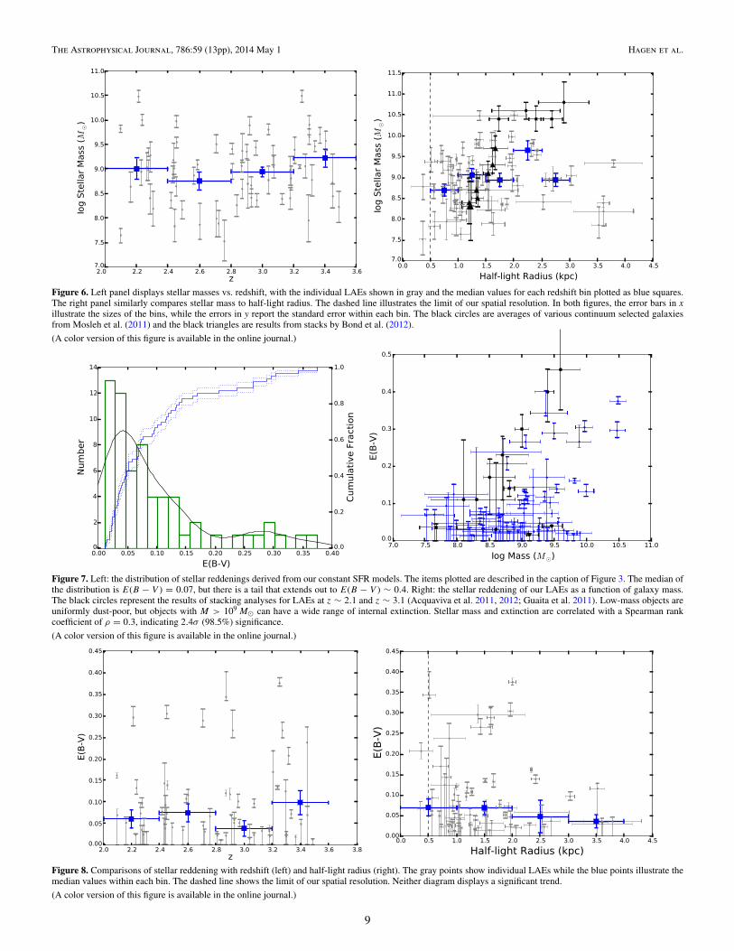
Figure 6 plots our derived stellar masses against two param-eters, LAE size and redshift. Neither shows a significant trend.While Bond et al. (2012) did find a correlation between mass andhalf-light radius, their analysis dealt with stacked images, not

7

The Astrophysical Journal, 786:59 (13pp), 2014 May 1 Hagen et al.

Figure 4. Lack of LAE size evolution with redshift. The gray points are individual measurements while the blue squares are binned medians. A bias in size measurementfrom cosmic surface brightness dimming would manifest as a decrease in half-light radius as (1 + z)4. There is no evidence for this effect.

(A color version of this figure is available in the online journal.)

Figure 5. Left: the distribution of masses for the HPS LAEs under the assumption of a constant star formation rate throughout history. The items plotted on the leftfigure are described in the caption of Figure 3. The distribution is very nearly flat in the log over three orders of magnitude. Right: a comparison of galaxy mass withLyα luminosity. There is no significant correlation between the two parameters, implying that the sample’s Lyα flux-limit does not propagate strongly into a constrainton stellar mass.

(A color version of this figure is available in the online journal.)

individual SEDs. Our null result also agrees with that found forsurveys of UV-bright galaxies in the same redshift range. LAEsizes (as measured in the UV continuum) and stellar masses donot seem to be related (e.g., Mosleh et al. 2011).

4.3. E(B − V )

Since Lyα photons resonantly scatter off interstellar hydro-gen, even a small amount of extinction can reduce the emergentemission-line flux by several orders of magnitude. Thus, it haslong been argued that LAEs are mostly young, metal-poor ob-jects with very little dust (e.g., Gawiser et al. 2006; Mao et al.2007). Nevertheless, evidence for the existence of dust withinLAEs has been seen in the work of Finkelstein et al. (2009)among others. As the left-hand panel of Figure 7 illustrates, our

data demonstrate that, indeed, most LAEs are dust-poor. Basedon our SED analyses, half of the HPS LAEs have internal stel-lar reddenings E(B − V ) < 0.07, though there is a tail thatextends all the way out to E(B − V ) ∼ 0.4. The median ofthe E(B − V ) distribution is 0.067+0.003

−0.018. Notably, all the high-extinction objects are drawn from the high-mass end of the LAEmass function: every LAE with E(B − V ) > 0.25 has a massgreater than ∼109 M�. This agrees with correlations betweenmass and extinction seen in both the local universe and at highredshift (e.g., Garn & Best 2010; Kashino et al. 2013).

Figure 8 displays our estimates of differential reddeningversus redshift and galaxy size. There are no significant trends ineither diagram. Unlike Guaita et al. (2011) and Acquaviva et al.(2011), we see no evidence for any change in the mean reddeningof the LAE population versus redshift, and, unlike Bond et al.

8

The Astrophysical Journal, 786:59 (13pp), 2014 May 1 Hagen et al.

Figure 6. Left panel displays stellar masses vs. redshift, with the individual LAEs shown in gray and the median values for each redshift bin plotted as blue squares.The right panel similarly compares stellar mass to half-light radius. The dashed line illustrates the limit of our spatial resolution. In both figures, the error bars in xillustrate the sizes of the bins, while the errors in y report the standard error within each bin. The black circles are averages of various continuum selected galaxiesfrom Mosleh et al. (2011) and the black triangles are results from stacks by Bond et al. (2012).

(A color version of this figure is available in the online journal.)

Figure 7. Left: the distribution of stellar reddenings derived from our constant SFR models. The items plotted are described in the caption of Figure 3. The median ofthe distribution is E(B − V ) = 0.07, but there is a tail that extends out to E(B − V ) ∼ 0.4. Right: the stellar reddening of our LAEs as a function of galaxy mass.The black circles represent the results of stacking analyses for LAEs at z ∼ 2.1 and z ∼ 3.1 (Acquaviva et al. 2011, 2012; Guaita et al. 2011). Low-mass objects areuniformly dust-poor, but objects with M > 109 M� can have a wide range of internal extinction. Stellar mass and extinction are correlated with a Spearman rankcoefficient of ρ = 0.3, indicating 2.4σ (98.5%) significance.

(A color version of this figure is available in the online journal.)

Figure 8. Comparisons of stellar reddening with redshift (left) and half-light radius (right). The gray points show individual LAEs while the blue points illustrate themedian values within each bin. The dashed line shows the limit of our spatial resolution. Neither diagram displays a significant trend.

(A color version of this figure is available in the online journal.)

9

The Astrophysical Journal, 786:59 (13pp), 2014 May 1 Hagen et al.

Figure 9. Left: the age distribution of the HPS LAEs. The ages extend over ∼2.5 dex. Right: the distribution of LAE ages vs. redshift, with individual objects plottedin gray and binned medians in blue. There is no evidence for evolution in the LAE population.

(A color version of this figure is available in the online journal.)

Figure 10. Dust-corrected UV star formation rate plotted against stellar massfor various high-redshift galaxies. Our luminous, spectroscopically selectedLAEs are shown in red, and narrow-band-selected LAEs from Vargas et al.(2014) are in pink. The blue and green points show higher-mass galaxies fromthe Rodighiero et al. (2011) survey of COSMOS and GOODS-N: blue arecontinuum-selected (BzK) galaxies, while green shows submillimeter brightsystems found by the Herschel-PACS instrument. The solid black line is thestar-forming “main sequence” defined by Daddi et al. (2007) for 1.5 < z < 2.5;the extrapolation of this line to lower SFRs is shown with a dashed line. LAEsand submillimeter galaxies lie above this relation, along the main sequencesfound by Whitaker et al. (2012) for z = 2.0 (lower dotted line) and z = 3.5(upper dotted line).

(A color version of this figure is available in the online journal.)

(2012), we see no correlation between E(B − V ) and half-lightradius. Again, we caution that the LAE samples consideredhere are more luminous than those derived from narrow-band surveys, and by studying individual, rather than stackedspectra, we are avoiding many of the systematic difficulties thatcomplicate the interpretation of previous measurements (Vargaset al. 2014).

4.4. Age

Figure 9 displays the age distribution for the HPS LAEs,under the simplest assumption of a constant SFR history. Thetwo figures together support the stacking analyses of Lai et al.

(2008), Guaita et al. (2011), and Acquaviva et al. (2011), whichargued that LAEs are relatively young, with ages between∼107 and 109 yr. The median age of the HPS sample islog t = 7.96+0.19

−0.14, and just ∼3% have ages greater than a Gyr.Interestingly, there no evidence for evolution in the sample. Thisdisagrees with result of Guaita et al. (2011), who found narrow-band selected z = 2.06 LAEs to be older and dustier than theirz = 3.1 counterparts. It is also in conflict with the re-analysis byAcquaviva et al. (2012), who concluded that these same LAEswere “growing younger” with time. A likely explanation for thisdiscrepancy lies in the details of the stacking procedure used byboth groups, as slight differences can produce discrepant results(see Vargas et al. 2014). Our analysis of individual LAEs avoidsthat pitfall.

4.5. Star Formation Rates and the Main Sequence of Galaxies

The observed SFR of an LAE can be derived several ways:from the luminosity of its Lyα emission line via the assumptionof Case B recombination,

SFR(Lyα) = 9.1 × 10−43 L(Lyα) M� yr−1 (2)

(Brocklehurst 1971; Kennicutt 1998), from the extinction-corrected flux density of the UV continuum between 1500 Åand 2800 Å,

SFR(UV) = 1.4 × 10−28 Lν M� yr−1 (3)

(Kennicutt 1998), and via the fit to the object’s SED (a valuewhich is largely dependent on the UV emission, but which mayalso include factors such as age).

Figure 10 plots our dust-corrected UV SFRs against stellarmass, and compares these data to those obtained from othersamples of high-z galaxies. From the figure, it is clear that eachselection technique identifies galaxies in a different region ofthe mass–SFR diagram. LAEs are primary low-mass, low-SFRobjects that lie above the star-forming main sequence found byDaddi et al. (2007), in a region of the diagram consistent withmeasurements of galaxy main-sequence evolution (Whitakeret al. 2012). Both IFU and narrow-band-selected LAEs fall inthis same region, confirming that both discovery techniques

10

The Astrophysical Journal, 786:59 (13pp), 2014 May 1 Hagen et al.

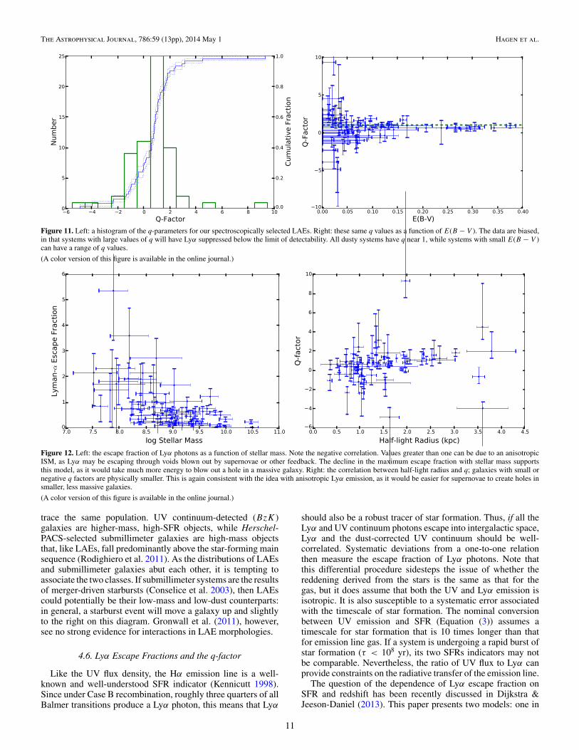
Figure 11. Left: a histogram of the q-parameters for our spectroscopically selected LAEs. Right: these same q values as a function of E(B − V ). The data are biased,in that systems with large values of q will have Lyα suppressed below the limit of detectability. All dusty systems have q near 1, while systems with small E(B − V )can have a range of q values.

(A color version of this figure is available in the online journal.)

Figure 12. Left: the escape fraction of Lyα photons as a function of stellar mass. Note the negative correlation. Values greater than one can be due to an anisotropicISM, as Lyα may be escaping through voids blown out by supernovae or other feedback. The decline in the maximum escape fraction with stellar mass supportsthis model, as it would take much more energy to blow out a hole in a massive galaxy. Right: the correlation between half-light radius and q; galaxies with small ornegative q factors are physically smaller. This is again consistent with the idea with anisotropic Lyα emission, as it would be easier for supernovae to create holes insmaller, less massive galaxies.

(A color version of this figure is available in the online journal.)

trace the same population. UV continuum-detected (BzK)galaxies are higher-mass, high-SFR objects, while Herschel-PACS-selected submillimeter galaxies are high-mass objectsthat, like LAEs, fall predominantly above the star-forming mainsequence (Rodighiero et al. 2011). As the distributions of LAEsand submillimeter galaxies abut each other, it is tempting toassociate the two classes. If submillimeter systems are the resultsof merger-driven starbursts (Conselice et al. 2003), then LAEscould potentially be their low-mass and low-dust counterparts:in general, a starburst event will move a galaxy up and slightlyto the right on this diagram. Gronwall et al. (2011), however,see no strong evidence for interactions in LAE morphologies.

4.6. Lyα Escape Fractions and the q-factor

Like the UV flux density, the Hα emission line is a well-known and well-understood SFR indicator (Kennicutt 1998).Since under Case B recombination, roughly three quarters of allBalmer transitions produce a Lyα photon, this means that Lyα

should also be a robust tracer of star formation. Thus, if all theLyα and UV continuum photons escape into intergalactic space,Lyα and the dust-corrected UV continuum should be well-correlated. Systematic deviations from a one-to-one relationthen measure the escape fraction of Lyα photons. Note thatthis differential procedure sidesteps the issue of whether thereddening derived from the stars is the same as that for thegas, but it does assume that both the UV and Lyα emission isisotropic. It is also susceptible to a systematic error associatedwith the timescale of star formation. The nominal conversionbetween UV emission and SFR (Equation (3)) assumes atimescale for star formation that is 10 times longer than thatfor emission line gas. If a system is undergoing a rapid burst ofstar formation (τ < 108 yr), its two SFRs indicators may notbe comparable. Nevertheless, the ratio of UV flux to Lyα canprovide constraints on the radiative transfer of the emission line.

The question of the dependence of Lyα escape fraction onSFR and redshift has been recently discussed in Dijkstra &Jeeson-Daniel (2013). This paper presents two models: one in

11

The Astrophysical Journal, 786:59 (13pp), 2014 May 1 Hagen et al.

which the escape fraction is independent of SFR, and a secondwhere the escape fraction decreases as the SFR increases. Wefind a significant inverse correlation between stellar mass andescape fraction, ρ = −0.54 (4.5σ or >99.999% significance)which supports the second model; this is shown in Figure 12.Unsurprisingly, the Lyα escape fraction also correlates withdifferential extinction, as mass and E(B − V ) are coupled (seeFigure 7). We note that the median escape fraction of our sample,∼0.5 (or 0.6, if we use the SED-based SFRs), is somewhat largerthan the 0.29 value found by Blanc et al. (2011) using the samesample of LAEs. Most of this difference is due to the use ofdeeper CANDELS data, which greatly improves the photometryand fixes the slope of the rest-frame UV.

Perhaps a more useful way of looking at the radiative transferproblem is through the variable q, which relates Lyα opticaldepth to that of the stellar continuum at 1216 Å. As defined byFinkelstein et al. (2008),

q = τLyα

τ1216, (4)

where τλ = 0.921 kλE(B − V ) and k1216 = 5.27 under theempirical reddening law described by Calzetti (2001). Figure 11shows the distribution of q values and the behavior of q withE(B − V ). Interestingly, at large reddenings q never gets muchabove 1, suggesting that in these systems, the Lyα emitting gasand the UV starlight are seeing the same amount of extinction.We do expect that galaxies with large Lyα optical depths will becensored out of our LAE sample. However, in dust-rich systemsit appears that, if Lyα escapes, it does so with very few resonantscatterings. This is consistent with models that involve strongwinds, such as that proposed by Verhamme et al. (2008). On theother hand, at low reddenings, we see a large range of q values.Systems with q < 0 imply anisotropic emission, a top-heavyIMF, or a very young starburst, where the UV luminosity to SFRconversion breaks down. As expected, we find that the half-lightradius and q-factor are positively correlated, with a Spearmanrank order coefficient of ρ = 0.35 (99.5% confidence). Thiscorrelation is shown in the right hand panel of Figure 12. A smallsize could lead to less homogeneity and thus more opportunitiesfor Lyα to undergo anisotropic radiative transfer.

5. CONCLUSION

Using broadband photometric data which extends from therest-frame UV through to the near-IR, we have been ableto measure the stellar masses, reddenings, and sizes for asample of 63 luminous LAEs found in the HPS. Our fitsdemonstrate that, contrary to popular belief, Lyα emitters arenot exclusively low-mass objects. In fact, HPS-selected LAEsare quite heterogeneous, and are drawn from almost the entirestellar mass range of high-redshift galaxies. Moreover, thereis a striking similarity between the mass function of LAEsand the mass function expected for the galactic star-formingpopulation as a whole. This fact, and the lack of correlationbetween Lyα luminosity and stellar mass, suggests that searchesfor Lyα emission are excellent way of sampling a large fractionof the mass function of high-redshift star-forming galaxies.

LAEs occupy a different part of stellar mass-SFR parameterspace than that of galaxies found by other methods. Like thehigher-mass submillimeter galaxies, LAEs fall above the mainsequence of star-forming galaxies found by Daddi et al. (2007).This suggests that there is a different slope for the main sequenceof star-bursting galaxies. Interestingly, LAEs do fall along the

main sequence defined by Whitaker et al. (2012), though the∼2 dex extrapolation required to reach their masses introducessignificant uncertainty. Due to the various selection effects atwork, the connection between the various classes of star-forminggalaxies is murky at best.

We also find that the range in observed q-factors is depen-dent on the reddening, with the widest range of q-values oc-curring at low extinction. Interestingly, the observed values ofq tend to unity as the reddening (or mass) increases, suggest-ing that in these objects, Lyα photons are not undergoing alarge number of scattering events. This strongly implies thatwinds are an important component in the making of high-massLAEs. Furthermore, we find that the half-light radius and theq-factor are positively correlated, implying that Lyα emission isenhanced in very small objects.

We thank the referee for helpful comments. We also thankJoshua Adams for the use of his photometry from the HET-DEX Pilot Survey. We acknowledge the Research Computerand Cyberinfrastructure Unit of Information Technology Ser-vices, and in particular W. Brouwer at The Pennsylvania StateUniversity for providing computational support and resourcesfor this project. This work is based on observations taken by theCANDELS Multi-Cycle Treasury Program with the NASA/ESA HST, which is operated by the Association of Universitiesfor Research in Astronomy, Inc., under NASA contract NAS5-26555. The work was also partially supported by NSF grantsAST 09-26641 and AST 10-55919. The Institute for Gravitationand the Cosmos is supported by the Eberly College of Scienceand the Office of the Senior Vice President for Research at thePennsylvania State University.

This research has made use of NASA’s Astrophysics DataSystem and the python packages IPython, NumPy, SciPy, andmatplotlib.

Facilities: CFHT, HST, Mayall, Smith, Spitzer (IRAC), Sub-aru, UH:2.2m, UKIRT

REFERENCES

Acquaviva, V., Gawiser, E., & Guaita, L. 2011, ApJ, 737, 47Acquaviva, V., Vargas, C., Gawiser, E., & Guaita, L. 2012, ApJL, 751, L26Adams, J. J., Blanc, G. A., Hill, G. J., et al. 2011, ApJS, 192, 5Atek, H., Siana, B., Scarlata, C., et al. 2011, ApJ, 743, 121Bell, E. F., & de Jong, R. S. 2001, ApJ, 550, 212Bertin, E., & Arnouts, S. 1996, A&AS, 117, 393Blanc, G. A., Adams, J. J., Gebhardt, K., et al. 2011, ApJ, 736, 31Bond, N. A., Gawiser, E., Gronwall, C., et al. 2009, ApJ, 705, 639Bond, N. A., Gawiser, E., Guaita, L., et al. 2012, ApJ, 753, 95Brocklehurst, M. 1971, MNRAS, 153, 471Brooks, S., & Gelman, A. 1998, J. Comp. Graph. Stat., 7, 434Bruzual, G., & Charlot, S. 2003, MNRAS, 344, 1000Calzetti, D. 2001, PASP, 113, 1449Capak, P., Aussel, H., Ajiki, M., et al. 2007, ApJS, 172, 99Chabrier, G. 2003, PASP, 115, 763Chonis, T. S., Blanc, G. A., Hill, G. J., et al. 2013, ApJ, 775, 99Conroy, C. 2013, ARA&A, 51, 393Conselice, C. J., Chapman, S. C., & Windhorst, R. A. 2003, ApJL, 596, L5Cowie, L. L., Barger, A. J., & Hu, E. M. 2010, ApJ, 711, 928Cowie, L. L., & Hu, E. M. 1998, ApJ, 115, 1319Daddi, E., Dickinson, M., Morrison, G., et al. 2007, ApJ, 670, 156Deharveng, J. M., Small, T., Barlow, T. A., et al. 2008, ApJ, 680, 1072Dijkstra, M., & Jeeson-Daniel, A. 2013, MNRAS, 435, 3333Donsker, M. 1952, Ann. Math. Statist., 23, 393Drory, N., Feulner, G., Bender, R., et al. 2001, MNRAS, 325, 550Efron, B. 1987, J. Am. Stat. Assoc., 397, 171Ferguson, H. C., Dickinson, M., Giavalisco, M., et al. 2004, ApJL, 600, L107

12

The Astrophysical Journal, 786:59 (13pp), 2014 May 1 Hagen et al.

Finkelstein, S. L., Hill, G. J., Gebhardt, K., et al. 2011, ApJ, 729, 140Finkelstein, S. L., Papovich, C., Dickinson, M., et al. 2013, Natur, 502, 524Finkelstein, S. L., Rhoads, J. E., Malhotra, S., & Grogin, N. 2009, ApJ,

691, 465Finkelstein, S. L., Rhoads, J. E., Malhotra, S., Grogin, N., & Wang, J. 2008, ApJ,

678, 655Garn, T., & Best, P. N. 2010, MNRAS, 409, 421Gawiser, E., Francke, H., Lai, K., et al. 2007, ApJ, 671, 278Gawiser, E., van Dokkum, P. G., Gronwall, C., et al. 2006, ApJL, 642, L13Gelman, A., & Rubin, D. 1992, StaSc, 7, 457Giavalisco, M., Ferguson, H. C., Koekemoer, A. M., et al. 2004, ApJL, 600, L93Grogin, N. A., Kocevski, D. D., Faber, S. M., et al. 2011, ApJS, 197, 35Gronwall, C., Bond, N. A., Ciardullo, R., et al. 2011, ApJ, 743, 9Gronwall, C., Ciardullo, R., Hickey, T., et al. 2007, ApJ, 667, 79Guaita, L., Acquaviva, V., Padilla, N., et al. 2011, ApJ, 733, 114Guaita, L., Gawiser, E., Padilla, N., et al. 2010, ApJ, 714, 255Hill, G. J., MacQueen, P. J., Smith, M. P., et al. 2008, Proc. SPIE, 7014, 231Hinshaw, G., Larson, D., Komatsu, E., et al. 2013, ApJS, 208, 19Hu, E. M., Cowie, L. L., Barger, A. J., et al. 2010, ApJ, 725, 394Hu, E. M., Cowie, L. L., & McMahon, R. G. 1998, ApJL, 502, L99Kashino, D., Silverman, J. D., Rodighiero, G., et al. 2013, ApJL, 777, L8Kauffmann, G., Heckman, T. M., White, S. D. M., et al. 2003, MNRAS,

341, 33Kennicutt, R. 1998, ARA&A, 36, 189Koekemoer, A. M., Faber, S. M., Ferguson, H. C., et al. 2011, ApJS, 197, 36Kroupa, P. 2001, MNRAS, 322, 231Lai, K., Huang, J.-S., Fazio, G., et al. 2008, ApJ, 674, 70Lewis, A., & Bridle, S. 2002, PhRvD, 66, 103511Lidman, C., Hayes, M., Jones, D. H., et al. 2012, MNRAS, 420, 1946Madau, P. 1995, ApJ, 441, 18Makovoz, D., & Marleau, F. 2005, PASP, 117, 1113Malhotra, S., Rhoads, J. E., Finkelstein, S. L., et al. 2012, ApJL, 750, L36Mao, J., Lapi, A., Granato, G. L., de Zotti, G., & Danese, L. 2007, ApJ,

667, 655McLinden, E. M., Rhoads, J. E., Malhotra, S., et al. 2014, MNRAS, 439, 446

Mosleh, M., Williams, R. J., Franx, M., & Kriek, M. 2011, ApJ, 727, 5Muzzin, A., Marchesini, D., Stefanon, M., et al. 2013, ApJ, 777, 18Nakajima, K., Ouchi, M., Shimasaku, K., et al. 2012, ApJ, 745, 12Nakajima, K., Ouchi, M., Shimasaku, K., et al. 2013, ApJ, 769, 3Nilsson, K. K., Ostlin, G., Moller, P., et al. 2011, A&A, 529, A9Ono, Y., Ouchi, M., Mobasher, B., et al. 2012, ApJ, 744, 83Ouchi, M., Shimasaku, K., Akiyama, M., et al. 2008, ApJS, 176, 301Ouchi, M., Shimasaku, K., Furusawa, H., et al. 2010, ApJ, 723, 869Papovich, C., Finkelstein, S. L., Ferguson, H. C., Lotz, J. M., & Giavalisco, M.

2011, MNRAS, 412, 1123Partridge, R., & Peebles, P. J. 1967, ApJ, 147, 868Pentericci, L., Grazian, A., Scarlata, C., et al. 2010, A&A, 514, A64Pierre, M., Valtchanov, I., Altieri, B., et al. 2004, JCAP, 09, 011Planck Collaboration, Ade, P. A. R., Aghanim, N., et al. 2013, A&A, in press

(arXiv:1303.5076)R Core Team 2012, R: A Language and Environment for Statistical Computing,

http://www.R-project.org/Rodighiero, G., Daddi, E., Baronchelli, I., et al. 2011, ApJL, 739, L40Salpeter, E. 1955, ApJ, 121, 161Schaerer, D., & de Barros, S. 2009, A&A, 502, 423Scott, D. 1992, Multivariate Density Estimation: Theory, Practice, and Visual-

ization (New York: Wiley)Scoville, N., Aussel, H., Brusa, M., et al. 2007, ApJS, 172, 1Shapley, A. E., Steidel, C. C., Pettini, M., & Adelberger, K. L. 2003, ApJ,

588, 65Song, M., Finkelstein, S. L., Gebhardt, K., et al. 2014, ApJ, submittedTomczak, A. R., Quadri, R. F., Tran, K.-V. H., et al. 2013, ApJ, 783, 85van Dokkum, P., Brammer, G., Momcheva, I., et al. 2013, arXiv:1305.2140Vargas, C. J., Bish, H., Acquaviva, V., et al. 2014, ApJ, 783, 26Verhamme, A., Dubois, Y., Blaizot, J., et al. 2012, A&A, 546, A111Verhamme, A., Schaerer, D., Atek, H., & Tapken, C. 2008, A&A, 491, 89Whitaker, K. E., van Dokkum, P. G., Brammer, G., & Franx, M. 2012, ApJL,

754, L29Yuma, S., Ohta, K., Yabe, K., et al. 2010, ApJ, 720, 1016Zibetti, S., Charlot, S., & Rix, H.-W. 2009, MNRAS, 400, 1181

13