spectral based solution methods - university of …mjm/spectral.solutions.pdfspectral based solution...

Spectral based solution methodsThis notebook has been written in Mathematica by

Mark J. McCreadyProfessor and Chair of Chemical EngineeringUniversity of Notre DameNotre Dame, IN 46556USA

[email protected]://www.nd.edu/~mjm/

It is copyrighted to the extent allowed by which ever laws pertain to the World Wide Web and the Internet.

I would hope that as a professional courtesy, this notice remain visible to other users. There is no charge for copying and dissemination.

Version: 11/25/98

Overview of the spectral approach

The basic ideal of anything "spectral" is the systematic representation/decomposition of a vector, function orsolution in terms of some basis vectors, functions which are independent (in this case orthogonal/biorthogonal).The basis vectors or functions must span the space and thus form a complete set so that any vector, function orsolution can be represented.

In symbolic form, we are interested in solving, L @y D = f HxL by representing f HxL in terms of our basis functionsand then ultimately finding y in terms of these same functions. Thus we are not directly finding the inverseoperator solution as we did in the Green's function approach, i.e., y = L -1 f HxL. We look for these expansions,

f HxL = ⁄ j=1n cj f j HxL

yHxL = ⁄ j=1n dj f j HxL

Presumably there will be a straightforward way of finding the cj ' ssince f HxL is a known function. (This will be toform an inner product.) We will find that we can obtain the dj 's by substituting all that we know in the equationand forming an inner product for each term.

Once we have defined the problem as the equation, L y = f HxL, and its boundary conditions, BHyL = 0. We need asystematic way to produce an appropriate set of basis functions. The best possible set will usually be obtainedfrom the eigenvalue problem, L y = -l y with BHyL = 0. For a self adjoint operator we will generate real l's andorthogonal eigenfunctions. If L is not self-adjoint, we can take advantage of biorthonality.

We will define the expansion of a term in the equation by expansion in terms of eigenfunctions as a Finite FourierTransform which is a linear operator and will, of course, have an inverse.

If we cannot readily solve L@ y D = -l y, we may instead use a known set of eigenfunctions from a differentoperator. This is effectively a numerical solution technique which we will discuss later.

Expansion of an arbitrary function in terms of a set of eigenfunctions.

ü Here are two functions that we would like to fit with our Eigenfunctions.

ff @x_ D : = x H1 - x2 Lgg@x_ D : = -x Hx - 2 x 2 + x3 L

2 spectral.solutions.nb

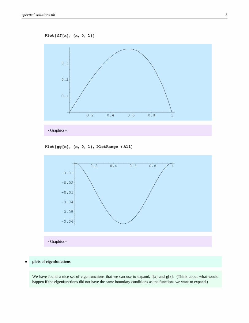
Plot @ff @xD, 8x, 0, 1 <D

0.2 0.4 0.6 0.8 1

0.1

0.2

0.3

Ü Graphics Ü

Plot @gg@xD, 8x, 0, 1 <, PlotRange Ø All D

0.2 0.4 0.6 0.8 1

-0.06

-0.05

-0.04

-0.03

-0.02

-0.01

Ü Graphics Ü

ü plots of eigenfunctions

We have found a nice set of eigenfunctions that we can use to expand, f[x] and g[x]. (Think about what wouldhappen if the eigenfunctions did not have the same boundary conditions as the functions we want to expand.)

spectral.solutions.nb 3

Plot @Sin @p xD, 8x, 0, 1 <D

0.2 0.4 0.6 0.8 1

0.2

0.4

0.6

0.8

1

Ü Graphics Ü

Plot @Sin @2 p xD, 8x, 0, 1 <D

0.2 0.4 0.6 0.8 1

-1

-0.5

0.5

1

Ü Graphics Ü

As they say, etc...


ü Here are our eigenfunctions

f@x_, i_ D : =è!!!

2 Sin @i p xD

ü Verify the orthonormality

‡0

1

psi @x, 1 D2 „x

‡0

1

psiHx, 1L2 „ x

‡0

1

psi @x, 3 D2 „x

‡0

1

psiHx, 3L2 „ x

‡0

1

psi @x, 1 D psi @x, 4 D „x

‡0

1

psiHx, 1L psiHx, 4L „ x

ü Now get the coefficients for ff[x]

We start with the assumed functional form for the expansion,

f HxL = „j=1

n

cj f j HxL

now form the inner product with the functionfk HxL

‡0

1

r HxL fk HxL f HxL „ x = ‡0

1

r HxL fk HxL ‚j=1

n

cj fj HxL „ x


On the right side we can switch the summation and integration Hassuming that everything will convergeL

‡0

1

r HxL fk HxL f HxL „ x = „j=1

n

‡0

1

r HxL fk HxL cj fj HxL „x

next just move the cj outside of the integration,

= „j=1

n

cj ‡0

1

r HxL fk HxL fj HxL „ x

For properly normalized orthogonalized functions the integral just equals dkj which means that the right side is just,

ck .

‡0

1

r HxL fk HxL f HxL „ x = ck .

For the eigenfunctions we have chosen, r(x) = 1. This gives then for ff[x], the first one and then a lot of others,

ü First expand ff[x]

‡0

1

ff @xD f@x, 1 D „x

6è!!!

2ÅÅÅÅÅÅÅÅÅÅÅÅÅÅÅÅÅÅÅÅÅÅÅ

p3

cks = Table @Integrate @ff @xD f@x, i D, 8x, 0, 1 <D, 8i, 1, 10 <D

9 6è!!!


p3, -

3ÅÅÅÅÅÅÅÅÅÅÅÅÅÅÅÅÅÅÅÅÅÅÅÅÅÅÅÅÅÅÅÅÅ2

è!!!2 p3

,2

è!!!2

ÅÅÅÅÅÅÅÅÅÅÅÅÅÅÅÅÅÅÅÅÅÅÅ9 p3

, -3

ÅÅÅÅÅÅÅÅÅÅÅÅÅÅÅÅÅÅÅÅÅÅÅÅÅÅÅÅÅÅÅÅÅÅÅÅÅ16

è!!!2 p3

,6

è!!!2

ÅÅÅÅÅÅÅÅÅÅÅÅÅÅÅÅÅÅÅÅÅÅÅÅÅÅ125p3

, -1


è!!!2 p3

,6

è!!!2


,

-3

ÅÅÅÅÅÅÅÅÅÅÅÅÅÅÅÅÅÅÅÅÅÅÅÅÅÅÅÅÅÅÅÅÅÅÅÅÅÅÅÅÅÅ128

è!!!2 p3

,2

è!!!2


, -3


è!!!2 p3

=

If you like numbers we have


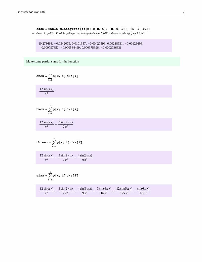
cksN = Table @NIntegrate @ff @xD f@x, i D, 8x, 0, 1 <D, 8i, 1, 10 <D— General::spell1 : Possible spelling error: new symbol name "cksN" is similar to existing symbol "cks".

80.273663,-0.0342079, 0.0101357,-0.00427599, 0.00218931,-0.00126696,0.000797852,-0.000534499, 0.000375396,-0.000273663<

Make some partial sums for the function

onex = ‚i =1

1

f@x, i D cks Pi T

12 sinHp xLÅÅÅÅÅÅÅÅÅÅÅÅÅÅÅÅÅÅÅÅÅÅÅÅÅÅÅÅÅÅÅÅÅÅÅÅÅÅÅ

p3

twox = ‚i =1

2

f@x, i D cks Pi T


p3-

3 sinH2 p xLÅÅÅÅÅÅÅÅÅÅÅÅÅÅÅÅÅÅÅÅÅÅÅÅÅÅÅÅÅÅÅÅÅÅÅÅÅÅÅÅÅ

2 p3

threex = ‚i =1

3

f@x, i D cks Pi T


p3-


2 p3+


9 p3

sixx = ‚i =1

6

f@x, i D cks Pi T


p3-


2 p3+


9 p3-


16p3+

12 sinH5 p xLÅÅÅÅÅÅÅÅÅÅÅÅÅÅÅÅÅÅÅÅÅÅÅÅÅÅÅÅÅÅÅÅÅÅÅÅÅÅÅÅÅÅÅÅÅÅ

125p3-

sinH6 p xLÅÅÅÅÅÅÅÅÅÅÅÅÅÅÅÅÅÅÅÅÅÅÅÅÅÅÅÅÅÅÅÅÅÅÅ

18p3


tenx = ‚i =1

10

f@x, i D cks Pi T


p3-


2 p3+


9 p3-


16p3+


125p3-


18p3+


343p3-


128p3+


243p3-

3 sinH10p xLÅÅÅÅÅÅÅÅÅÅÅÅÅÅÅÅÅÅÅÅÅÅÅÅÅÅÅÅÅÅÅÅÅÅÅÅÅÅÅÅÅÅÅÅÅÅ

250p3

We plot to see that it takes only about 3 terms

plt1 = Plot @8onex, twox, threex, sixx, tenx <, 8x, 0, 1 <D

0.2 0.4 0.6 0.8 1

0.1

0.2

0.3

0.4

Ü Graphics Ü


plt2 = Plot @ff @xD, 8x, 0, 1 <, PlotStyle -> Dashing @8.01, .02 <DD

0.2 0.4 0.6 0.8 1

0.1

0.2

0.3

Ü Graphics Ü

Show@plt1, plt2 D

0.2 0.4 0.6 0.8 1

0.1

0.2

0.3

0.4

Ü Graphics Ü

ü Now do gg

‡0

1

gg@xD f@x, 1 D „x


4è!!!

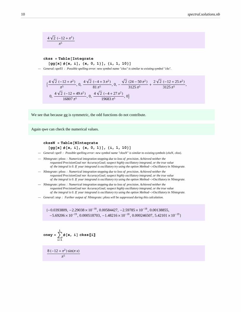
2 H-12+ p2LÅÅÅÅÅÅÅÅÅÅÅÅÅÅÅÅÅÅÅÅÅÅÅÅÅÅÅÅÅÅÅÅÅÅÅÅÅÅÅÅÅÅÅÅÅÅÅÅÅÅÅÅÅÅÅÅÅÅÅÅÅÅÅ

p5

ckss = Table @Integrate@gg@xD f@x, i D, 8x, 0, 1 <D, 8i, 1, 10 <D— General::spell1 : Possible spelling error: new symbol name "ckss" is similar to existing symbol "cks".

9 4è!!!

2 H-12+ p2LÅÅÅÅÅÅÅÅÅÅÅÅÅÅÅÅÅÅÅÅÅÅÅÅÅÅÅÅÅÅÅÅÅÅÅÅÅÅÅÅÅÅÅÅÅÅÅÅÅÅÅÅÅÅÅÅÅÅÅÅÅÅÅ

p5, 0,

4è!!!

2 H-4 + 3 p2LÅÅÅÅÅÅÅÅÅÅÅÅÅÅÅÅÅÅÅÅÅÅÅÅÅÅÅÅÅÅÅÅÅÅÅÅÅÅÅÅÅÅÅÅÅÅÅÅÅÅÅÅÅÅÅÅÅÅÅÅÅÅÅÅÅ

81p5, 0, -

è!!!2 H24- 50p2L

ÅÅÅÅÅÅÅÅÅÅÅÅÅÅÅÅÅÅÅÅÅÅÅÅÅÅÅÅÅÅÅÅÅÅÅÅÅÅÅÅÅÅÅÅÅÅÅÅÅÅÅÅÅÅÅÅÅÅÅÅÅ3125p5

+2

è!!!2 H-12+ 25p2L

ÅÅÅÅÅÅÅÅÅÅÅÅÅÅÅÅÅÅÅÅÅÅÅÅÅÅÅÅÅÅÅÅÅÅÅÅÅÅÅÅÅÅÅÅÅÅÅÅÅÅÅÅÅÅÅÅÅÅÅÅÅÅÅÅÅÅÅÅÅÅÅÅÅ3125p5

,

0,4

è!!!2 H-12+ 49p2L


, 0,4

è!!!2 H-4 + 27p2L

ÅÅÅÅÅÅÅÅÅÅÅÅÅÅÅÅÅÅÅÅÅÅÅÅÅÅÅÅÅÅÅÅÅÅÅÅÅÅÅÅÅÅÅÅÅÅÅÅÅÅÅÅÅÅÅÅÅÅÅÅÅÅÅÅÅÅÅÅÅ19683p5

, 0=

We see that because gg is symmetric, the odd functions do not contribute.

Again qwe can check the numerical values.

ckssN = Table @NIntegrate@gg@xD f@x, i D, 8x, 0, 1 <D, 8i, 1, 10 <D— General::spell : Possible spelling error: new symbol name "ckssN" is similar to existing symbols8cksN, ckss<.— NIntegrate::ploss : Numerical integration stopping due to loss of precision. Achieved neither the

requested PrecisionGoal nor AccuracyGoal; suspect highly oscillatory integrand, or the true valueof the integral is 0. If your integrand is oscillatory try using the option Method->Oscillatory in NIntegrate.

— NIntegrate::ploss : Numerical integration stopping due to loss of precision. Achieved neither therequested PrecisionGoal nor AccuracyGoal; suspect highly oscillatory integrand, or the true valueof the integral is 0. If your integrand is oscillatory try using the option Method->Oscillatory in NIntegrate.

— NIntegrate::ploss : Numerical integration stopping due to loss of precision. Achieved neither therequested PrecisionGoal nor AccuracyGoal; suspect highly oscillatory integrand, or the true valueof the integral is 0. If your integrand is oscillatory try using the option Method->Oscillatory in NIntegrate.

— General::stop : Further output of NIntegrate::ploss will be suppressed during this calculation.

8-0.0393809,-2.29038µ 10-18, 0.00584427,-2.59785µ 10-18, 0.00138855,-5.69206µ 10-19, 0.000518703,-1.48216µ 10-18, 0.000246507, 5.42101µ 10-19<

oney = ‚i =1

1

f@x, i D ckss Pi T

8 H-12+ p2L sinHp xLÅÅÅÅÅÅÅÅÅÅÅÅÅÅÅÅÅÅÅÅÅÅÅÅÅÅÅÅÅÅÅÅÅÅÅÅÅÅÅÅÅÅÅÅÅÅÅÅÅÅÅÅÅÅÅÅÅÅÅÅÅÅÅÅÅÅÅÅÅÅÅÅÅÅÅ

p5


twoy = ‚i =1

2

f@x, i D ckss Pi T— General::spell1 : Possible spelling error: new symbol name "twoy" is similar to existing symbol "twox".


p5

sixy = ‚i =1

6

f@x, i D ckss Pi T— General::spell1 : Possible spelling error: new symbol name "sixy" is similar to existing symbol "sixx".


p5+

8 H-4 + 3 p2L sinH3 p xLÅÅÅÅÅÅÅÅÅÅÅÅÅÅÅÅÅÅÅÅÅÅÅÅÅÅÅÅÅÅÅÅÅÅÅÅÅÅÅÅÅÅÅÅÅÅÅÅÅÅÅÅÅÅÅÅÅÅÅÅÅÅÅÅÅÅÅÅÅÅÅÅÅÅÅÅÅÅÅÅÅÅÅ

81 p5+

è!!!2

ikjjjjj-

è!!!2 H24- 50p2L


+2

è!!!2 H-12+ 25p2L


y{zzzzz sinH5 p xL

teny = ‚i =1

10

f@x, i D ckss Pi T— General::spell1 : Possible spelling error: new symbol name "teny" is similar to existing symbol "tenx".


p5+

8 H-4 + 3 p2L sinH3 p xLÅÅÅÅÅÅÅÅÅÅÅÅÅÅÅÅÅÅÅÅÅÅÅÅÅÅÅÅÅÅÅÅÅÅÅÅÅÅÅÅÅÅÅÅÅÅÅÅÅÅÅÅÅÅÅÅÅÅÅÅÅÅÅÅÅÅÅÅÅÅÅÅÅÅÅÅÅÅÅÅÅÅÅ

81 p5+

è!!!2

ikjjjjj-

è!!!2 H24- 50p2L


+2

è!!!2 H-12+ 25p2L


y{zzzzz sinH5 p xL +

8 H-12+ 49p2L sinH7 p xLÅÅÅÅÅÅÅÅÅÅÅÅÅÅÅÅÅÅÅÅÅÅÅÅÅÅÅÅÅÅÅÅÅÅÅÅÅÅÅÅÅÅÅÅÅÅÅÅÅÅÅÅÅÅÅÅÅÅÅÅÅÅÅÅÅÅÅÅÅÅÅÅÅÅÅÅÅÅÅÅÅÅÅÅÅÅÅÅÅÅÅÅ

16807 p5+

8 H-4 + 27p2L sinH9 p xLÅÅÅÅÅÅÅÅÅÅÅÅÅÅÅÅÅÅÅÅÅÅÅÅÅÅÅÅÅÅÅÅÅÅÅÅÅÅÅÅÅÅÅÅÅÅÅÅÅÅÅÅÅÅÅÅÅÅÅÅÅÅÅÅÅÅÅÅÅÅÅÅÅÅÅÅÅÅÅÅÅÅÅÅÅÅÅÅ

19683 p5

This one converges real fast also.


Plot @8gg@xD, oney, twoy, sixy, teny <, 8x, 0, 1 <D

0.2 0.4 0.6 0.8 1

-0.06

-0.05

-0.04

-0.03

-0.02

-0.01

Ü Graphics Ü

ü Now do one with non homogeneous boundary conditions:

‡0

1 H1 - ff @xDL f@x, 1 D „x

-6

è!!!2

ÅÅÅÅÅÅÅÅÅÅÅÅÅÅÅÅÅÅÅÅÅÅÅp3

+2

è!!!2

ÅÅÅÅÅÅÅÅÅÅÅÅÅÅÅÅÅÅÅÅÅÅÅp

ckss = Table @Integrate@H1 - ff @xDL f@x, i D, 8x, 0, 1 <D, 8i, 1, 10 <D

9-6

è!!!2

ÅÅÅÅÅÅÅÅÅÅÅÅÅÅÅÅÅÅÅÅÅÅÅp3

+2

è!!!2

ÅÅÅÅÅÅÅÅÅÅÅÅÅÅÅÅÅÅÅÅÅÅÅp

,3

ÅÅÅÅÅÅÅÅÅÅÅÅÅÅÅÅÅÅÅÅÅÅÅÅÅÅÅÅÅÅÅÅÅ2

è!!!2 p3

, -2

è!!!2

ÅÅÅÅÅÅÅÅÅÅÅÅÅÅÅÅÅÅÅÅÅÅÅ9 p3

+2

è!!!2

ÅÅÅÅÅÅÅÅÅÅÅÅÅÅÅÅÅÅÅÅÅÅÅ3 p

,3


è!!!2 p3

, -6

è!!!2


+2

è!!!2


,

1ÅÅÅÅÅÅÅÅÅÅÅÅÅÅÅÅÅÅÅÅÅÅÅÅÅÅÅÅÅÅÅÅÅÅÅÅÅ18

è!!!2 p3

, -6

è!!!2


+2

è!!!2


,3


è!!!2 p3

, -2

è!!!2


+2

è!!!2


,3


è!!!2 p3

=

Again qwe can check the numerical values.


ckssN = Table @NIntegrate@H1 - ff @xDL f@x, i D, 8x, 0, 1 <D, 8i, 1, 10 <D— General::spell1 : Possible spelling error: new symbol name "ckssN" is similar to existing symbol "ckss".

80.626653, 0.0342079, 0.28997, 0.00427599, 0.177874, 0.00126696, 0.127819,0.000534499, 0.0996598, 0.000273663<

onez = ‚i =1

1

f@x, i D ckss Pi T

è!!!2

ikjjjjj-

6è!!!


p3+

2è!!!


p

y{zzzzz sinHp xL

twoz = ‚i =1

2

f@x, i D ckss Pi T

è!!!2

ikjjjjj-

6è!!!


p3+

2è!!!


p

y{zzzzz sinHp xL +


2 p3

sixz = ‚i =1

6

f@x, i D ckss Pi T

è!!!2

ikjjjjj-

6è!!!


p3+

2è!!!


p

y{zzzzz sinHp xL +


2 p3+

è!!!2

ikjjjjj-

2è!!!

2ÅÅÅÅÅÅÅÅÅÅÅÅÅÅÅÅÅÅÅÅÅÅÅ9 p3

+2

è!!!2




16p3+

è!!!2

ikjjjjj-

6è!!!

2ÅÅÅÅÅÅÅÅÅÅÅÅÅÅÅÅÅÅÅÅÅÅÅÅÅÅ125p3

+2

è!!!2




18p3


tenz = ‚i =1

10

f@x, i D ckss Pi T

è!!!2

ikjjjjj-

6è!!!


p3+

2è!!!


p

y{zzzzz sinHp xL +


2 p3+

è!!!2

ikjjjjj-

2è!!!

2ÅÅÅÅÅÅÅÅÅÅÅÅÅÅÅÅÅÅÅÅÅÅÅ9 p3

+2

è!!!2




16p3+

è!!!2

ikjjjjj-

6è!!!


+2

è!!!2




18p3+

è!!!2

ikjjjjj-

6è!!!


+2

è!!!2




128p3+

è!!!2

ikjjjjj-

2è!!!


+2

è!!!2



3 sinH10p xLÅÅÅÅÅÅÅÅÅÅÅÅÅÅÅÅÅÅÅÅÅÅÅÅÅÅÅÅÅÅÅÅÅÅÅÅÅÅÅÅÅÅÅÅÅÅ

250p3

This one does not converge very well because the boundary conditions cannot be met. We get the "ringing" that isshown in figure 3.7 of V&M.

Think of the consequences of this observation for our problem below.

Plot @8H1 - ff @xDL, onez, twoz, sixz, tenz <, 8x, 0, 1 <D

0.2 0.4 0.6 0.8 1

0.2

0.4

0.6

0.8

1

Ü Graphics Ü


‡ Summary of function expansion

To recap, our function is known (at least symbolically) and we choose a set of known eigenfunctions from aconvenient operator. The expansion is easily accomplished by forming the inner product which directly givesvalues of the expansion coefficients for, say,f HxL = ⁄ j=1

n cj f j HxL.


Finite Fourier transform

Now we are ready to solve an inhomogenous ODE with a spectral expansion in terms of the eigenfunctions foryHxL andf HxL.A simple example equation (3.19.1) in V&M isd2 yÅÅÅÅÅÅÅÅÅÅÅÅÅdx2 - U2 y = - f HxL , xœ(0,L)

with yH0L = y HLL = 0.

The obvious eigenfunctions for this problem come from the eigenvalue problem,

d2 fÅÅÅÅÅÅÅÅÅÅÅÅÅÅdx2 = - l f , with, fH0L = fHLL = 0, which we have already solved.

The differential operator, L[•] , is then d2 •ÅÅÅÅÅÅÅÅÅÅÅÅ

dx2 although as V&M show, it could also bed2 •ÅÅÅÅÅÅÅÅÅÅÅÅdx2 - U2 • with no real problem.

We choose, d2 fÅÅÅÅÅÅÅÅÅÅÅÅÅÅ

dx2 = - l f and know that the normalized eigenfunctions are,

fnHxL = "######2ÅÅÅÅÅÅL SinH npxÅÅÅÅÅÅÅÅÅÅÅÅL L , n = 1, 2, ...

**Our presumption is that the answer will be: y@xD = F-1[yn ] = ⁄n=1¥ yn fn***

Here we go starting with:

L@yD - U2 y = - f HxL , we form the inner product of both sides of the equation with fnHxL by multiplying andintegrating

Ÿ0

Lfn L@yD „ x - U2 Ÿ0

Lfn y „ x = - Ÿ0

Lfn f HxL „ x (eq1)

We will define an operator called the finite Fourier Transform, F[•] such that:

F[•] = Ÿ0

LrHxL fn • „ x. In this problem,r HxL = 1.

From this definition and what we know about expanding an arbitray function and also knowing that L@fD = - lf ,

We rearrange eq1 into

U2 Ÿ0

Lfn y „ x =U2 F[y(x)] =U2yn

- Ÿ0

Lfn f HxL „ x = - F[ f HxL] = - fn

finally we have the term, Ÿ0

LfnHxL L@yHxLD „ x .

Since the complete problem is self adjoint, (fnHxL, L@yHxLD) = (y, L@fnHxLD), we have


Ÿ0

LfnHxL L@yHxLD „ x = Ÿ0

Ly HxL L@fnHxLD „ x

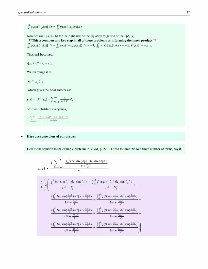
Now we use L[f]=- lf for the right side of the equation to get rid of theL@fnHxLD **This a common and key step in all of these problems as is forming the inner product **

Ÿ0

LfnHxL L@yHxLD „ x = Ÿ0

Ly HxL H-ln fnHxLL „ x = -ln Ÿ0

Ly HxL H fnHxLL „ x = -lnF[y(x)] = -lnyn.

Thus eq1 becomes:

-(ln+ U2) yn = -fn .

We rearrange it as

yn = fnÅÅÅÅÅÅÅÅÅÅÅÅÅÅÅÅÅÅÅÅÅÅÅÅHln + U2

which gives the final answer as:

yHxL = F-1[yn] = ‚n=1

∞ fnÅÅÅÅÅÅÅÅÅÅÅÅÅÅÅÅÅÅÅÅÅÅÅÅHln + U2 fn

or if we substitute everything,

2 „n=1

∞ IŸ0

Lf @t D Sin A n p t

ÅÅÅÅÅÅÅÅÅÅÅÅÅÅÅÅL E „t M Sin @ n p xÅÅÅÅÅÅÅÅÅÅÅÅÅÅÅÅL D

ÅÅÅÅÅÅÅÅÅÅÅÅÅÅÅÅÅÅÅÅÅÅÅÅÅÅÅÅÅÅÅÅÅÅÅÅÅÅÅÅÅÅÅÅÅÅÅÅÅÅÅÅÅÅÅÅÅÅÅÅÅÅÅÅÅÅÅÅÅÅÅÅÅÅÅÅÅU2 + n2 p2

ÅÅÅÅÅÅÅÅÅÅÅÅÅÅÅÅÅÅÅÅÅL2ÅÅÅÅÅÅÅÅÅÅÅÅÅÅÅÅÅÅÅÅÅÅÅÅÅÅÅÅÅÅÅÅÅÅÅÅÅÅÅÅÅÅÅÅÅÅÅÅÅÅÅÅÅÅÅÅÅÅÅÅÅÅÅÅÅÅÅL

ü Here are some plots of our answer

Here is the solution to the example problem in V&M, p. 275. I need to limit this to a finite number of terms, say 8.

ans1 =

2 „n=1

8 IŸ0

Lf @t D Sin A n p tÅÅÅÅÅÅÅÅÅÅÅÅL E „t M Sin @ n p xÅÅÅÅÅÅÅÅÅÅÅÅL D

ÅÅÅÅÅÅÅÅÅÅÅÅÅÅÅÅÅÅÅÅÅÅÅÅÅÅÅÅÅÅÅÅÅÅÅÅÅÅÅÅÅÅÅÅÅÅÅÅÅÅÅÅÅÅÅÅÅÅÅÅÅÅÅÅÅÅÅU2 + n2 p2

ÅÅÅÅÅÅÅÅÅÅÅÅÅÅL2

ÅÅÅÅÅÅÅÅÅÅÅÅÅÅÅÅÅÅÅÅÅÅÅÅÅÅÅÅÅÅÅÅÅÅÅÅÅÅÅÅÅÅÅÅÅÅÅÅÅÅÅÅÅÅÅÅÅÅÅÅÅÅÅÅÅÅÅÅÅÅÅÅÅÅÅÅÅÅÅÅÅÅÅÅÅÅÅÅÅÅÅÅÅL

1ÅÅÅÅÅÅÅL

ikjjjjjjj2

ikjjjjjjj

IŸ0

Lf HtL sinH p tÅÅÅÅÅÅÅÅÅL L „ tM sinH p xÅÅÅÅÅÅÅÅÅÅL L

ÅÅÅÅÅÅÅÅÅÅÅÅÅÅÅÅÅÅÅÅÅÅÅÅÅÅÅÅÅÅÅÅÅÅÅÅÅÅÅÅÅÅÅÅÅÅÅÅÅÅÅÅÅÅÅÅÅÅÅÅÅÅÅÅÅÅÅÅÅÅÅÅÅÅÅÅÅÅÅÅÅÅÅÅÅÅÅÅÅÅÅÅÅÅÅÅÅÅÅÅU2 + p2

ÅÅÅÅÅÅÅÅÅL2

+IŸ0

Lf HtL sinH 2 p tÅÅÅÅÅÅÅÅÅÅÅÅÅL L „ tM sinH 2 p xÅÅÅÅÅÅÅÅÅÅÅÅÅÅL L

ÅÅÅÅÅÅÅÅÅÅÅÅÅÅÅÅÅÅÅÅÅÅÅÅÅÅÅÅÅÅÅÅÅÅÅÅÅÅÅÅÅÅÅÅÅÅÅÅÅÅÅÅÅÅÅÅÅÅÅÅÅÅÅÅÅÅÅÅÅÅÅÅÅÅÅÅÅÅÅÅÅÅÅÅÅÅÅÅÅÅÅÅÅÅÅÅÅÅÅÅÅÅÅÅÅÅÅÅÅU2 + 4 p2

ÅÅÅÅÅÅÅÅÅÅÅÅÅL2

+

IŸ0




+IŸ0



ÅÅÅÅÅÅÅÅÅÅÅÅÅÅÅÅL2

+

IŸ0




+IŸ0




+

IŸ0




+IŸ0




y{zzzzzzz

y{zzzzzzz


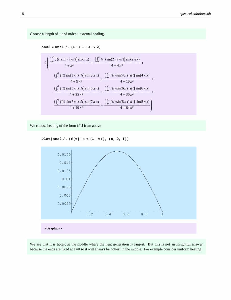
Choose a length of 1 and order 1 external cooling,

ans2 = ans1 ê. 8L -> 1, U -> 2<

2ikjjjjjjj

IŸ0

1f HtL sinHp tL „ tM sinHp xL

ÅÅÅÅÅÅÅÅÅÅÅÅÅÅÅÅÅÅÅÅÅÅÅÅÅÅÅÅÅÅÅÅÅÅÅÅÅÅÅÅÅÅÅÅÅÅÅÅÅÅÅÅÅÅÅÅÅÅÅÅÅÅÅÅÅÅÅÅÅÅÅÅÅÅÅÅÅÅÅÅÅÅÅÅÅÅÅÅÅÅÅÅÅÅÅÅ4 + p2

+IŸ0

1f HtL sinH2 p tL „ tM sinH2 p xL

ÅÅÅÅÅÅÅÅÅÅÅÅÅÅÅÅÅÅÅÅÅÅÅÅÅÅÅÅÅÅÅÅÅÅÅÅÅÅÅÅÅÅÅÅÅÅÅÅÅÅÅÅÅÅÅÅÅÅÅÅÅÅÅÅÅÅÅÅÅÅÅÅÅÅÅÅÅÅÅÅÅÅÅÅÅÅÅÅÅÅÅÅÅÅÅÅÅÅÅÅÅÅÅÅÅÅÅÅÅ4 + 4 p2

+

IŸ0



+IŸ0


ÅÅÅÅÅÅÅÅÅÅÅÅÅÅÅÅÅÅÅÅÅÅÅÅÅÅÅÅÅÅÅÅÅÅÅÅÅÅÅÅÅÅÅÅÅÅÅÅÅÅÅÅÅÅÅÅÅÅÅÅÅÅÅÅÅÅÅÅÅÅÅÅÅÅÅÅÅÅÅÅÅÅÅÅÅÅÅÅÅÅÅÅÅÅÅÅÅÅÅÅÅÅÅÅÅÅÅÅÅ4 + 16p2

+

IŸ0



+IŸ0



+

IŸ0



+IŸ0



y{zzzzzzz

We choose heating of the form ff[t] from above

Plot @ans2 ê. 8f @t D -> t H1 - t L<, 8x, 0, 1 <D

0.2 0.4 0.6 0.8 1

0.0025

0.005

0.0075

0.01

0.0125

0.015

0.0175

Ü Graphics Ü

We see that it is hotest in the middle where the heat generation is largest. But this is not an insightful answerbecause the ends are fixed at T=0 so it will always be hottest in the middle. For example consider uniform heating


Plot @ans2 ê. 8f @t D -> 1<, 8x, 0, 1 <D

0.2 0.4 0.6 0.8 1

0.02

0.04

0.06

0.08

Ü Graphics Ü

Let's try to mess it up a bit with heating that is strongest at the ends,

Plot @ans2 ê. 8f @t D -> 1 - t H1 - t L<, 8x, 0, 1 <D

0.2 0.4 0.6 0.8 1

0.01

0.02

0.03

0.04

0.05

0.06

0.07

Ü Graphics Ü

Let's see if this last one changes much if the number of terms is reduced.


ans3 =

2 „n=1

4 IŸ0

Lf @t D Sin A n p tÅÅÅÅÅÅÅÅÅÅÅÅL E „t M Sin @ n p xÅÅÅÅÅÅÅÅÅÅÅÅL D

ÅÅÅÅÅÅÅÅÅÅÅÅÅÅÅÅÅÅÅÅÅÅÅÅÅÅÅÅÅÅÅÅÅÅÅÅÅÅÅÅÅÅÅÅÅÅÅÅÅÅÅÅÅÅÅÅÅÅÅÅÅÅÅÅÅÅÅU2 + n2 p2

ÅÅÅÅÅÅÅÅÅÅÅÅÅÅL2

ÅÅÅÅÅÅÅÅÅÅÅÅÅÅÅÅÅÅÅÅÅÅÅÅÅÅÅÅÅÅÅÅÅÅÅÅÅÅÅÅÅÅÅÅÅÅÅÅÅÅÅÅÅÅÅÅÅÅÅÅÅÅÅÅÅÅÅÅÅÅÅÅÅÅÅÅÅÅÅÅÅÅÅÅÅÅÅÅÅÅÅÅÅL

1ÅÅÅÅÅÅÅL

ikjjjjjjj2

ikjjjjjjj

IŸ0

Lf HtL sinH p tÅÅÅÅÅÅÅÅÅL L „ tM sinH p xÅÅÅÅÅÅÅÅÅÅL L

ÅÅÅÅÅÅÅÅÅÅÅÅÅÅÅÅÅÅÅÅÅÅÅÅÅÅÅÅÅÅÅÅÅÅÅÅÅÅÅÅÅÅÅÅÅÅÅÅÅÅÅÅÅÅÅÅÅÅÅÅÅÅÅÅÅÅÅÅÅÅÅÅÅÅÅÅÅÅÅÅÅÅÅÅÅÅÅÅÅÅÅÅÅÅÅÅÅÅÅÅU2 + p2

ÅÅÅÅÅÅÅÅÅL2

+IŸ0




+

IŸ0




+IŸ0




y{zzzzzzz

y{zzzzzzz

ans4 = ans3 ê. 8L -> 1, U -> 2<

2ikjjjjjjj

IŸ0

1f HtL sinHp tL „ tM sinHp xL

ÅÅÅÅÅÅÅÅÅÅÅÅÅÅÅÅÅÅÅÅÅÅÅÅÅÅÅÅÅÅÅÅÅÅÅÅÅÅÅÅÅÅÅÅÅÅÅÅÅÅÅÅÅÅÅÅÅÅÅÅÅÅÅÅÅÅÅÅÅÅÅÅÅÅÅÅÅÅÅÅÅÅÅÅÅÅÅÅÅÅÅÅÅÅÅÅ4 + p2

+IŸ0



+

IŸ0



+IŸ0



y{zzzzzzz

Plot @ans4 ê. 8f @t D -> 1 - t H1 - t L<, 8x, 0, 1 <D

0.2 0.4 0.6 0.8 1

0.01

0.02

0.03

0.04

0.05

0.06

0.07

Ü Graphics Ü

Here we compare the solution with f[t] = 1-t(1-t) for 4 terms and 8 terms. There is not much difference perhapsbecause the end regions, where the fit to f(t) is not easy to do, does not contribute too much. You may wish tocheck this further.


Show@%32, %D

0.2 0.4 0.6 0.8 1

0.01

0.02

0.03

0.04

0.05

0.06

0.07

Ü Graphics Ü

‡ Summary of Finite Fourier transform technique

From the form of the ode, L@yD = - f HxL (Note that original equation could also be L@yD + by = - f HxL becauseit leads to the same eigenvalue problem.) and boundary conditions we formulate L[ f]=- lf and solve (using the same boundary conditions) to get the basis functions (A complete set ofeigenfunctions that will be able to represent any finite function or solution).

We then presume a spectral solution form of y[x] = F-1[yn] = ⁄n=1∞ yn fn.

We take the Finite Fourier transform of each term in the equation. This means form the inner product: (ODE,fn).

a. Any term that contains a factor, say b, multipling y will just yield b F[y(x)] = b yn

b. Any term with a precribed inhomogeneous function becomes, F[ f HxL] = fn (and we know how to expand any function.

c. The one term that requires manipulation is, Ÿ0

LfnHxL L@yHxLD „ x, which know came from (fnHxL, L@yHxLD)

and thus must be equal, for our self adjoint equation to, (yHxL, L@fnHxLD). This is just, (yHxL, -ln fnHxL) or in termsof the definition of F[y(x)] it becomes, -ln yn

d. Just solve this equation for yn and then transform back to get y[x],

yHxL = F-1[yn] = ⁄n=1∞ yn fn

e. Substitute what you need.


spectral based solution methods - university of …mjm/spectral.solutions.pdfspectral based solution...

Documents