specification of a stochastic simulation model for ... · wp/06/268 specification of a stochastic...

WP/06/268

Specification of a Stochastic Simulation Model for Assessing Debt Sustainability

in Emerging Market Economies

Doug Hostland and Philippe Karam

© 2006 International Monetary Fund WP/06/268 IMF Working Paper IMF Institute

Specification of a Stochastic Simulation Model

for Assessing Debt Sustainability in Emerging Market Economies

Prepared by Doug Hostland and Philippe Karam1

Authorized for distribution by Ralph Chami

December 2006

Abstract This Working Paper should not be reported as representing the views of the IMF. The views expressed in this Working Paper are those of the author(s) and do not necessarily represent those of the IMF or IMF policy. Working Papers describe research in progress by the author(s) and are published to elicit comments and to further debate.

This paper documents the specification of a model that was constructed to assess debt sustainability in emerging market economies. Key features of the model include external and fiscal sectors, which allow assessment of external and public debt in a unified framework; public and external debt, which both have an explicit maturity structure along with a distinction between denomination in domestic versus foreign currency to facilitate debt management analysis; monetary and fiscal policy, which are endogenous and specified using explicit forward-looking policy rules; an endogenous risk premium on public and external debt; and a mechanism for invoking a sudden stop in private capital flows. The paper provides an overview of the basic structure of the model, outlines the methodology used to calibrate the parameters, and illustrates the key properties of the model with reference to dynamic responses of selected variables to shocks of interest. JEL Classification Numbers: C15, C61, H62, H63 Keywords: Debt sustainability, dynamic analysis, Monte Carlo simulations. Author’s E-Mail Address: [email protected], [email protected]

1 This is a companion paper to a previously issued IMF Working Paper 05/226, “Assessing Debt Sustainability in Emerging Market Economies Using Stochastic Simulation Methods,” by the same authors. Doug Hostland is a Senior Economist in the Development Economics Vice Presidency of the World Bank; Philippe Karam is an economist at the IMF Institute. We thank Ms. Lei Lei Myaing and Ms. Pinn Siraprapasiri for providing research assistance, and Ms. Asmahan Bedri and Ms. Yasmina Zinbi for their editorial help.

- 2 -

Contents Page

I. Overview ................................................................................................................................3

II. Model Structure.....................................................................................................................4 A. The Foreign Sector....................................................................................................5 B. The Domestic Sector .................................................................................................8 C. The Fiscal Sector.....................................................................................................12 D. The External Sector.................................................................................................14

III. Calibration Methodology...................................................................................................16 A. Calibration of the Parameters..................................................................................17

IV. Model Properties................................................................................................................20 A. The Benchmark Specification.................................................................................20 B. Alternative Fiscal Policy Rules ...............................................................................21 C. Alternative Monetary Policy Rules .........................................................................22 D. Foreign-Currency-Denominated Debt ....................................................................22 E. Endogenous Default Premium.................................................................................23 F. Exchange Rate Response to the External Debt Burden...........................................23

V. Conclusions.........................................................................................................................23

References................................................................................................................................32 Tables Table 1: Volatility of Simulated Variables ..............................................................................18 Figures Figure 1. Dynamic Response to Adverse Aggregate Demand Shock-Benchmark Scenario...25 Figure 2. Dynamic Response with Alternative Fiscal Policy Rules ........................................27 Figure 3. Dynamic Response with Less Aggressive Monetary Policy Rule ...........................28 Figure 4. Dynamic Response with Foreign Currency Denominated Debt ..............................29 Figure 5. Dynamic Response with Endogenous Risk Premium ..............................................30

- 3 -

I. OVERVIEW

Debt sustainability plays a central role in economic policy analysis in emerging market economies. The standard framework used by the IMF and the World Bank to assess debt sustainability basically entails conducting stress tests with reference to a baseline projection scenario.2 The framework largely consists of accounting identities, with few economic (behavioral) relationships. The stress tests are therefore difficult to interpret from an economic perspective. A number of recent studies have addressed this shortcoming by applying stochastic simulation methods to economic models (notably, Barnhill and Kopits, 2003; Garcia and Rigobon, 2004, and Mendoza and Oviedo, 2003). This approach generates explicit probability measures that take into account interaction among key economic variables, which provides insight into the likelihood that the debt burden will rise over the projection period. Our companion paper (Hostland and Karam, 2005) extended this line of research by investigating how various modeling specification issues affect probability measures generated using stochastic simulation methods. Four features were found to have a major influence: (1) monetary and fiscal policy; (2) financial fragility (reliance on short-term, foreign currency borrowing); (3) an endogenous default premium; and (4) “sudden stops” in private capital flows. This paper documents the specification of a stochastic simulation model that incorporates each of these features. Monetary and fiscal policy have often been major contributing factors to financial crises in emerging market economies over the past few decades and, hence, play a central role in our analysis. Monetary and fiscal policy are endogenous in the model, implemented using forward-looking policy rules. Our previous research (Hostland and Karam, 2005) has shown how a well-designed fiscal planning strategy can be used to help manage the risks surrounding debt sustainability over the medium term. The current paper illustrates that the response of monetary policy to shocks also has a significant impact on public and external debt burdens. Monetary and fiscal policies are therefore an integral element in assessing debt sustainability in our modeling framework. Debt management also plays a prominent role in our analysis. External and public debt have explicit maturity structures and include a distinction between debt denominated in foreign versus domestic currency, enabling one to vary the degree of financial fragility. In addition, the cost of issuing (external and public) debt includes a default premium, which responds endogenously to changes in the debt burden. The intuition here is that lenders are concerned about borrowers’ “willingness to repay”; a higher debt burden is therefore perceived to increase the risk of debt default. The default premium cannot rise above a threshold level, above which debt default is perceived as being imminent. This invokes a “sudden stop” in

2 This is documented in IMF (2002 and 2003). A similar framework has been adopted by the IMF and World Bank (2004a and 2004b) to assess debt sustainability in low-income countries.

- 4 -

private capital flows. We believe that these features play a prominent role in assessing debt sustainability in emerging market economies. The macroeconomic core model consists of a few reduced-form equations for aggregate demand/supply dynamics and the inflation process. Our preference for a small, aggregate model is largely driven by computational requirements of stochastic simulation methods. In addition, such a (reduced-form) specification enables us to focus on key parameters of interest and greatly facilitates calibration of the model and sensitivity analysis. Some equations in the model are specified based on theoretical grounds. For example, the exchange rate is determined by the uncovered interest parity condition, and the term structure of interest rates is modeled using the expectations hypothesis. Expectations are formed by combining backward- and forward-looking components, so as to encompass purely adaptive and rational (model-consistent) mechanisms as two extremes. The parameters of the model are calibrated to match selected time-series properties of the data. This entails setting parameters to values such that the variables simulated by the model have variances and autocorrelations that correspond as close as possible to those observed in the data. For instance, the forward- and backward-looking components of expectations are combined such that the variance and autocorrelation of the exchange rate and interest rates simulated by the model match those observed in the data. A fair amount of judgment is also added to the calibration exercise. The next section of the paper describes the basic structure of the model. Section III discusses the calibration of the model, section IV illustrates some of the model’s key simulation properties, and Section V offers conclusions.

II. MODEL STRUCTURE

The model has foreign and domestic sectors, allowing an impact in foreign economic developments and terms of trade to affect a (generic) domestic open economy. Real output and real interest rates are decomposed into transitory and permanent components. The permanent components have a stochastic trend. The transitory components are interpreted as deviations from equilibrium levels. All variables converge to their respective equilibrium levels (the permanent components) in the long run. This ensures that the cyclical components are stationary. The monetary and fiscal authorities in the model can distinguish between the transitory and permanent components. Hence, there is no uncertainty about the source or persistence of the shocks encountered. The model can be simulated, however, such that policymakers cannot immediately ascertain whether observed changes to output and real interest rates are transitory or permanent. We will present the foreign and domestic sectors of the model, each in turn.

- 5 -

A. The Foreign Sector

The foreign sector of the model comprises five stochastic equations along with several identities. Aggregate Supply/Demand Dynamics The cyclical component of foreign real output c

tyf (the foreign “output gap”) is modeled using the following reduced-form equation:

1 1 2 1 3 1c c c c

t t t t t tyf yf E yf rf fα α α ε− += + + + , ( F.1 )

where c

trf is the cyclical component of the foreign real cost of funds and 21 1(0, )t ffε σ is a

random error term. Output dynamics are determined by an autoregressive component 1c

tyf − and a forward-looking component 1

ct tE yf + , generated in a model-consistent manner. Output

(and inflation) exhibit persistence in the model. This reflects the view that various frictions associated with price and wage setting prevent product markets from clearing instantaneously. The cyclical component of the real cost of funds is defined as a weighted average of real yields on short- and long-term bonds, given by: 1 40(1 )c c c

t t trf rf rfυ υ= + − , where 1c

trf and 40ctrf represent the cyclical components of the real yield on 1-period and 40-

period bonds. The model is specified at the quarterly frequency so that 1ctrf corresponds to

the yield on 3-month treasury bills and 40ctrf corresponds to the real yield on 10-year discount

bonds. The Inflation Process The foreign inflation rate tpf∆ is determined by simultaneous interaction between the reaction of the monetary authority to economic developments and the formation of inflation expectations:

1 1 2 1 3 4 4 2( ) ,c c e esst t t t t t tpf yf yf pf pf pf fβ β β β ε− − +∆ = + + ∆ + ∆ + ∆ + ( F.2 )

- 6 -

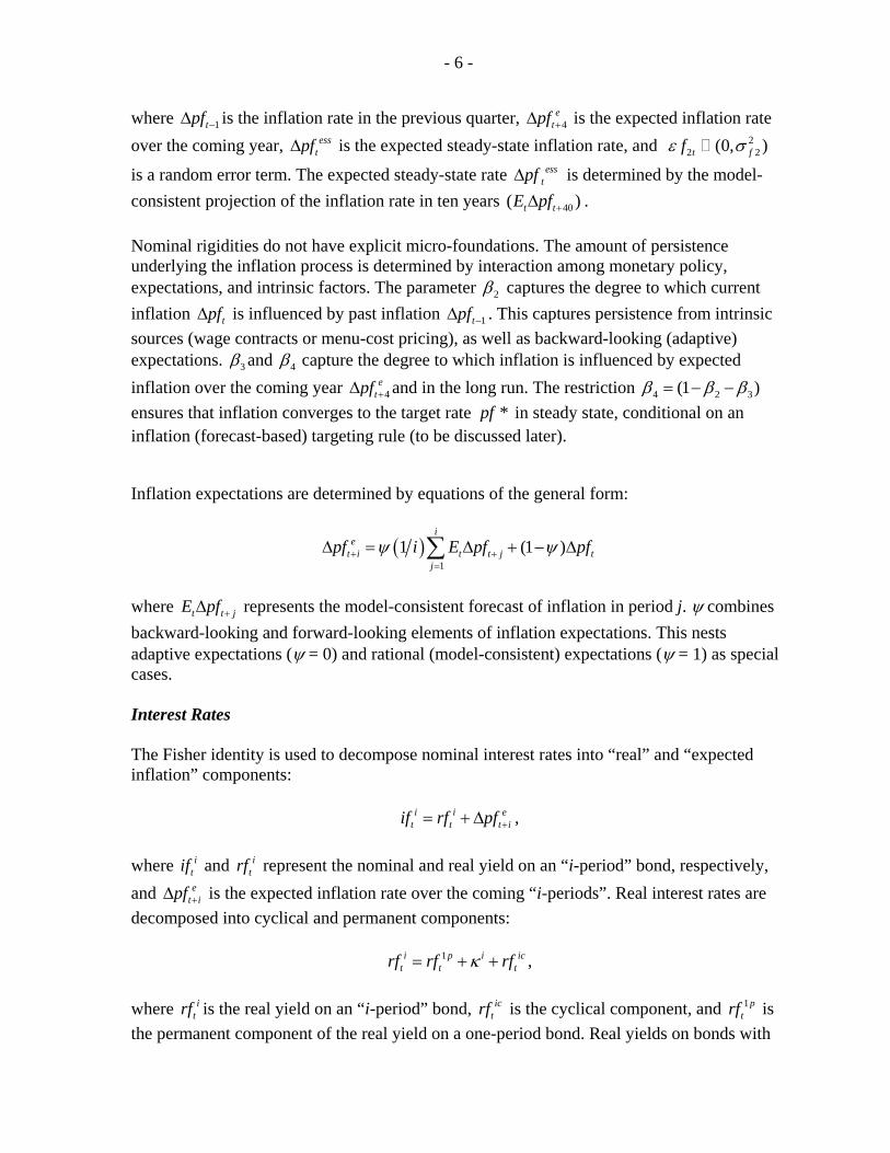
where 1tpf −∆ is the inflation rate in the previous quarter, 4e

tpf +∆ is the expected inflation rate over the coming year, ess

tpf∆ is the expected steady-state inflation rate, and 22 2(0, )t ffε σ

is a random error term. The expected steady-state rate esstpf∆ is determined by the model-

consistent projection of the inflation rate in ten years 40( )t tE pf +∆ . Nominal rigidities do not have explicit micro-foundations. The amount of persistence underlying the inflation process is determined by interaction among monetary policy, expectations, and intrinsic factors. The parameter 2β captures the degree to which current inflation tpf∆ is influenced by past inflation 1tpf −∆ . This captures persistence from intrinsic sources (wage contracts or menu-cost pricing), as well as backward-looking (adaptive) expectations. 3β and 4β capture the degree to which inflation is influenced by expected inflation over the coming year 4

etpf +∆ and in the long run. The restriction 4 2 3(1 )β β β= − −

ensures that inflation converges to the target rate *pf in steady state, conditional on an inflation (forecast-based) targeting rule (to be discussed later).

Inflation expectations are determined by equations of the general form:

( )1

1 (1 )i

et i t t j t

jpf i E pf pfψ ψ+ +

=

∆ = ∆ + − ∆∑

where t t jE pf +∆ represents the model-consistent forecast of inflation in period j. ψ combines backward-looking and forward-looking elements of inflation expectations. This nests adaptive expectations (ψ = 0) and rational (model-consistent) expectations (ψ = 1) as special cases. Interest Rates The Fisher identity is used to decompose nominal interest rates into “real” and “expected inflation” components: i i e

t t t iif rf pf += + ∆ , where i

tif and itrf represent the nominal and real yield on an “i-period” bond, respectively,

and et ipf +∆ is the expected inflation rate over the coming “i-periods”. Real interest rates are

decomposed into cyclical and permanent components:

1i p i ict t trf rf rfκ= + + ,

where i

trf is the real yield on an “i-period” bond, ictrf is the cyclical component, and 1p

trf is the permanent component of the real yield on a one-period bond. Real yields on bonds with

- 7 -

different maturities differ by a constant term premium iκ , which ranges from 25 basis points at one year ( )4 0.25κ = to 100 basis points at ten years ( )40 1.0κ = . The permanent component of the one-period real interest rate evolves stochastically over time as a random walk:

1 11 3

p pt t trf rf fε−= + , ( F.3 )

where 2

3 3(0, )t ffε σ is a random error term. The cyclical component is determined by monetary policy. Monetary Policy Monetary policy is set each period using a forward-looking policy rule:3

( )1 * 11 3 1 2 3 1 4

c c ct t t t t t trf E pf pf pf yf rf fγ γ γ ε+ − −⎡ ⎤= − − ∆ + + +⎣ ⎦ , ( F.4 )

where 1γ captures the monetary authority’s response to the expected deviation in the inflation rate over the coming year ( )3 1t t tE pf pf+ −− from the inflation target *pf∆ ; 2γ captures the response to the output gap; and 3γ captures the “interest rate smoothing” aspect of monetary policy, which is often motivated by the need to preserve orderly financial markets by limiting interest rate and exchange rate volatility.4 The random error term 2

4 4(0, )t ffε σ reflects the idea that the monetary authority cannot control short-term interest rates with certainty. The monetary policy rule (F.4) is a general specification that encompasses a number of special cases, notably a Taylor rule and an Inflation Forecast Based (IFB) rule.5 Rewriting the term

3 Although the monetary policy rule (F.4) is specified with reference to the short-term real interest rate 1c

trf ,

one can interpret the short-term nominal interest rate 1ctif as the “instrument” of monetary policy. This simply

entails substituting the Fisher identity 1 11

et t tif rf pf += + ∆ into the reaction function (F.4).

4 High values of 3γ dampen volatility in short-term interest rates, but delays the monetary policy response to shocks. See Taylor (1999b) and Sack and Wieland (1999).

5 The first rule is referred to as the Taylor rule, following Taylor (1993) in which a simple interest rate reaction function depended on contemporaneous values for inflation and output gap. A second type of monetary rule, an IFB rule, is a more forward-looking version of the Taylor rule where a short-term policy rate responds to a forecast of future inflation rather than the contemporaneous level of inflation. See Svensson (2003) for a critique of these rules.

- 8 -

above ( ) *3 1t t tE pf pf pf+ −⎡ ⎤− − ∆⎣ ⎦ , as ( ) *

4t t t tE pf pf pfτ τ τ+ + − +⎡ ⎤− − ∆⎣ ⎦ , where ( )4t tpf pfτ τ+ + −− is the year-on-year gross CPI inflation rate τ quarters into the future, (F.4) becomes the original Taylor (1993) when 1 2 0.5γ γ= = , and 3γ and τ are set to zero where no inertia is allowed. By contrast, when 0τ > , we refer to the rule as an IFB rule. The Term Structure of Interest Rates The term structure of interest rates is modeled using the expectations hypothesis:

( ) ( ) ( ) ( )1 1 4 51

1 1 1i

j i iit t t j it t t

jrf i E rf rf f fϕ κ ϕ υ ε υ ε+ −

=

⎡ ⎤= + + − + + −⎢ ⎥

⎣ ⎦∑ , ( F.5 )

where itrf is the expected real yield on an “i-period” discount bond, ( )1t t jE rf + is the

expected real yield on one-period bonds “j-periods” in the future and 24 4(0, )t ffε σ and

25 5(0, )t ffε σ are random error terms.ϕ combines forward- and backward-looking

components of expectations (as in the case of inflation expectations). In the case where 1ϕ = , the expected real yield on an “i-period” bond is determined by model-consistent

forecasts of future yields on the one-period bond plus a constant term premium iκ . In the case where 0ϕ = , expectations are static ( )1 1 1t t j tE rf rf+ −= . The two random error terms

4tfε and 5tfε enable us to calibrate the model to be consistent with the empirical finding that long-term interest rates fluctuate by more than what is predicted by the expectations hypothesis with rational expectations. Note that the formation of inflation expectations used to define real interest rates can differ from those used in the inflation equations. This enables us to consider the possibility that inflation expectations in financial markets are more (or less) forward-looking than those underlying the wage/price setting process.

B. The Domestic Sector

Aggregate Supply/Demand Dynamics The domestic sector of the model is essentially an open-economy version of the foreign sector. The cyclical component of output ty (the “output gap”) is influenced by cyclical movements in real interest rates, the real exchange rate, the stance of fiscal policy and foreign aggregate demand conditions:

3

1 1 2 1 3 4 5 6 7 10

c c c c ct t t t t j t j t t t t

j

y y E y r q yf pbal ttrα α α α τ α α α ε− + −=

= + + + + + ∆ + ∆ +∑ , ( 1 )

- 9 -

where c

tr is the cyclical component of the real cost of funds, tq is the real exchange rate,

tpbal is the primary budget balance as a percentage of GDP, ctyf is the cyclical component

of the foreign output, tttr is the terms of trade ( )x mp p with the export and import prices

modeled below using an error correction specification, and 21 1(0, )tε σ is a random error

term. The cyclical component of the real cost of funds ctr is determined by a combination of

short- and long-term interest rates: ( )1 401c c c

t t tr r rυ υ= + − , where 1c

tr and 40ctr represent the cyclical components of the real yield on one-period and 40-

period (10-year) discount bonds, respectively. The trend component of output p

ty (potential output) evolves over time as a random walk with a time-varying drift component tµ :

2pt t ty µ ε∆ = + ( 2 )

3t tµ ε∆ = + , ( 3 )

where 2

2 2(0, )tε σ and 23 3(0, )tε σ are random error terms.

The Inflation Process Inflation is determined in the same manner as in the foreign sector, with the addition of import prices:

3

1 1 2 1 3 4 4 5 40

( )c c e esst t t t t t j t j t

j

p y y p p p rpmβ β β β β τ ε− − + −=

∆ = + + ∆ + ∆ + ∆ + ∆ +∑ , ( 4 )

where rpm is the relative price of imports (the influence of this variable reflects the open economy’s status of the domestic sector), and changes influence inflation with lags.

24 4(0, )tε σ is a random error term.

Inflation expectations are generated along the same lines as in the foreign sector:

( )1

1 (1 )i

et i t t j t

j

p i E p pψ ψ+ +=

∆ = ∆ + − ∆∑ .

- 10 -

The expected steady-state inflation rate ess

tp∆ is determined by the model-consistent projection of inflation rate in ten years ( )40t tE p +∆ . Interest Rates Interest rates are determined along the same lines as in the foreign sector, with the addition of a time-varying risk premium on external and public debt. The Fisher condition decomposes nominal interest rates into “real” and “expected inflation” components:

( )( )4i it t t t i ti r E i p p+= + − .

Real interest rates are decomposed into permanent and cyclical components:

1i p i ict t tr r rκ= + + ,

where i

tr is the real yield on an “i-period” bond, ictr is its cyclical component, 1p

tr is the permanent component of the real yield on one-period bonds and iκ is a constant term premium. The permanent component of the real yield on one-period bonds 1p

tr differs from its foreign counterpart 1p

trf by a time-varying risk premium edtχ :

1 1p p edt t tr rf χ= + ,

Where ‘ed’ denotes external debt and edχ evolves over time according to:

* *1 1 2( ) ( )ed ss

t t ta edebt edebt b a pdebt pdebtχ χ= + − + − . ( 5 )

On the other hand, a time-varying risk premium related to public debt ‘pd’ is written as:

* *2 2 1( ) ( )pd ss

t t ta pdebt pdebt b a edebt edebtχ χ= + − + − , ( 6 )

where ssχ is the steady state level of the risk premium on external debt; pd

tχ is the risk premium on public debt. 1b is the portion of external debt issued by the public sector; and 2b is the portion of public debt issued abroad. The intuition underlying equations (5) and (6) is as follows: The risk premium on the private sector portion of external debt 1(1 )b− increases as the external debt burden rises above its initial level: *

1( )ssta edebt edebtχ + − , where 1a

represents foreign investors’ subjective perception of the default risk. Similarly, the risk premium on the domestic portion of public debt 2(1 )b− increases as the public debt burden

- 11 -

rises above its initial level: *2 ( )ta pdebt pdebt− , where 2a represents domestic investors’

subjective perception of the default risk. The risk premium on the foreign portion of public debt 1( )b includes both of the terms listed above:

* *1 2( ) ( )ss

t ta edebt edebt a pdebt pdebtχ + − + − , combining domestic and foreign investors’ subjective perception of the default risk. Monetary Policy The monetary policy rule in the domestic sector is the same as in the foreign sector:

( )1 * 11 3 1 2 3 1 5

c c ct t t t t t tr E p p p y rγ γ γ ε+ − −⎡ ⎤= − − ∆ + + +⎣ ⎦ , ( 7 )

where 2

5 5(0, )tε σ is the random error term. The Term Structure of Interest Rates The term structure of interest rates is modeled using the expectations hypothesis with constant term premia:

( ) ( ) ( )1 1 5 61

1 (1 ) (1 ) 0 1i

j i iit t t j it t t

jr E r riϕ κ ϕ υ ε υ ε ϕ+ −

=

⎡ ⎤= + + − + + − ≤ ≤⎢ ⎥

⎣ ⎦∑ , ( 8 )

where itr is the expected real yield on an “i-period” discount bond, ( )1t t jE r + is the model-consistent forecast of the real yield on one-period bonds “j-periods” in the future, and

25 5(0, )tε σ and 2

6 6(0, )tε σ are (mutually independent) random error terms. These last terms are introduced to make the model more consistent with the empirical finding that long-term interest rates fluctuate by more than what is predicted by the expectations hypothesis with rational expectations. The Exchange Rate The expected change in the real exchange rate 1

etq +∆ is determined by:6

6 To clarify, tq represents the (log of the) price of foreign exchange (expressed in real terms) so that an increase

in tq implies a real exchange rate depreciation. The real exchange rate tq equals ( )t fs p p− + , where p

and fp are the (log of the) domestic and foreign price levels and ts denotes the (log of the ) nominal exchange rate expressed as domestic currency per unit of foreign currency.

- 12 -

( ) ( )1 1 *1 14e ed

t t t t t tq r rf E edebt edebtχ θ+ +∆ = − − + − , ( 9 )

where ( )1 1 ed

t t tr rf χ− − is the domestic-foreign real interest rate differential that takes into

account a risk premium on external debt edtχ , and ( )*

1t tE edebt edebt+ − is the expected deviation in the external debt burden from its initial level. Expectations are modeled using a combination of backward- and forward-looking components:

( )1 1 11et t t tq E q qϕ ϕ+ + −= + − ( )0 1ϕ≤ ≤ ,

where 1t tE q + is the model-consistent forecast of the real exchange rate in the coming period and 1tq − is the lagged value. In the case where the external debt burden is expected to be at

its initial level ( )*1t tE edebt edebt+ = , equation (9) collapses to the uncovered interest rate

parity condition: ( )1 11 4e ed

t t t tq r rf χ+∆ = − − . When the external debt burden is expected to rise

above its initial level ( )*1t tE edebt edebt+ > , the real exchange rate is expected to depreciate.

The exchange rate depreciation improves the current account, reducing the deviation in the external debt burden from the initial level. This mechanism serves to limit the amount of volatility in the current account and external debt burden (discussed later in the paper).

C. The Fiscal Sector

Debt Service Debt service payments are defined with reference to the implicit interest rate on public debt

dti and the stock of public debt tD :

*d

t t tDS i D= .

In order to capture the exact relationship between movements in interest rates, the stock of debt and debt service costs, one would have to keep track of yields on all financial assets and liabilities held by the government at each point in time. We make a number of simplifying assumptions to reduce the computational burden. We abstract from interest-earning assets held by the government to equate net and gross public debt. The maturity structure of public debt is held constant so that the implicit interest rate can be calculated as a weighted average of current and lagged interest rates on government securities with different maturity dates. The weights reflect two factors. First, new debt issues are financed by bonds with different maturities. Second, interest rate payments are made on outstanding bonds that were issued at different dates in the past. We approximate the maturity structure by focusing on five maturity categories ranging from one quarter (90-day treasury bills) to 20 years. The implicit interest rate can be then approximated by:

- 13 -

( )( ) ( )

( ) ( )

81 4 4 4 4 8

1 4 1 2 3 8 11

20 4020 40

20 1 40 11 1

1 4 1 8

1 20 1 40 ,

dt t t t t t t j

j

t j t jj j

i i i i i i i

i i

ω ω ω

ω ω

− − − − +=

− + − += =

= + + + + +

+ +

∑

∑ ∑

where k

ti represents the (when issued) yield on a k-period bond issued in period “t” and the weights iω represent the proportion of outstanding bonds of each maturity i . The intuition underlying the above equation is as follows: One-period bonds mature each period so that the implicit interest rate on one-period bonds is simply the current short-term interest rate 1

ti . One-quarter of the one-year bonds mature each quarter so that the implicit interest rate is given by the average yield on one-year bonds issued in the current period and in the previous three quarters. Primary Fiscal Balance The primary fiscal balance, pbal , has a discretionary and a nondiscretionary component: d c

t t tpbal pbal pbal= + . The cyclical component c

tpbal moves in a countercyclical manner to capture the automatic stabilization properties of various tax and spending programs:

c ct tpbal yς= .

The discretionary component d

tpbal is determined by a fiscal policy rule. The fiscal authority aims to keep the debt-to-GDP ratio from rising over the medium term in the presence of uncertainty about future economic and fiscal developments. This is implemented using a forward-looking reaction function:

( ) ( )*1

d sst t tpbal pbal E pdebt pdebtλ +− = − , ( 10 )

where ( )d ss

tpbal pbal− represents the deviation of the discretionary component of the primary balance from its steady state level (expressed as proportions of GDP) and ( )*

1t tE pdebt pdebt+ − represents the expected deviation of the debt-to-GDP ratio from its

initial level in the coming quarter. The steady state level of the primary balance sstpbal is

determined by:

- 14 -

*( ) (1 )ss ss ss sspbal r g g pdebt⎡ ⎤= − + ∗⎣ ⎦ ,

where ssr and ssg represent the steady-state real interest rate and real growth rate. The fiscal policy rule (10) can be thought of as a control mechanism for attaining a debt target over the long run.

D. The External Sector

In Hostland and Karam (2005), we find that the pricing of traded goods had a significant influence on the sustainability of external debt. An exchange rate depreciation can result in a rapid improvement in the trade balance in our model mainly when traded goods are priced in foreign currency. The adjustment largely occurs through trade prices, not volumes. In the case where exports are priced in domestic currency, the adjustment largely occurs through trade volumes. The empirical evidence indicates that trade volumes adjust more slowly than trade prices. This makes the trade balance respond more gradually to exchange rate changes. We illustrate the importance of trade pricing by comparing simulations with exports priced in foreign versus domestic currency (Hostland and Karam, 2005, Table 3, p.24, simulations 6 and 6a, respectively). The simulation results indicate that pricing exports in domestic rather than foreign currency raises the amount of variability in the trade balance significantly. When exports are priced in domestic currency, the response of the trade balance to the exchange rate is sensitive to the trade price elasticity. The elasticity must be large enough so that an exchange rate depreciation improves the current account, otherwise the solvency condition will be violated.7 To summarize, an exchange rate depreciation affects the trade balance through the following channels: trade volumes, trade prices, and consumer prices. The latter interacts with the role that the monetary policy plays in allowing an impact of an exchange rate depreciation on wages and consumer prices, where a greater pass-through onto prices will induce less external adjustment and greater trade balance volatility. Trade Volumes The dynamic adjustments of import and export volumes (m and x) are specified in logarithmic form using an error correction specification (recall, all lower case variables are measured in logs scaled by a factor of 100, with the exception of a few variables such as the interest rate and the growth rate of GDP) :

7 This can be thought of in terms of the “extended Marshall-Lerner Conditions (MLC)” as in Hostland and Schembri (2005).

- 15 -

( )11 12 1 1 1 7t dt t t m t m t tm y rpm m y rpmα α λ β η ε− − −∆ = ∆ + ∆ − − − + ( 11a )

( )21 22 1 1 1 8t dt t t x t m t tx y rpx x yf rpxα α λ β η ε− − −∆ = ∆ + ∆ − − − + , ( 11b )

where yd and yf are domestic and foreign income and 2

7 7(0, )tε σ and 28 8(0, )tε σ are the

random error terms. The variables mrp and xrp represent the relative price of imports and exports defined by:

m m drp p p= − ( 12a )

x x frp p e p= − − , ( 12b )

where mp is the price of imports, dp is the price of the domestic consumption basket—a proxy price of import substitutes at home, xp is the price of exports (in domestic currency: a foreign country point of view), e is the nominal exchange rate and, fp is the price of the foreign consumption basket (in foreign currency). The error correction dynamics underlying equations (11a) and (11b) are calibrated to match the empirical evidence which indicates that trade volumes respond gradually to changes in relative prices ( )and m xη η (as per the

Marshall-Lerner Condition) and income ( )and m xβ β . Trade Prices Import and export prices are also modeled using an error correction specification to capture slow adjustment:

1( )essmt t mt m tp p p eρ φ−∆ = ∆ − ∆ − ∆ ( 13a )

1( )essxt t xt x tp pf p eρ φ−∆ = ∆ − ∆ − ∆ , ( 13b )

where ess

tp∆ and esstpf∆ represent the domestic and foreign steady-state inflation rate,

respectively, which are assumed to be exogenous, and ρ represents the dynamic error correction coefficient. The parameters ( )and m xφ φ determine the long-run effect of exchange

rate changes on import and export prices. Setting ( )1m xφ φ= = implies that exports and imports are priced in foreign currency (the small open economy assumption.) It implies that all exchange rate movements are ultimately passed-through into the domestic prices of traded

- 16 -

goods, or in other words, exchange rate movements have no effect on the terms of trade ( )x mp p . Setting ( )1mφ = and ( )0xφ = implies producer currency pricing for exports only (as is the case under the classic MLC). In this case, exchange rate changes affect import prices (there is full exchange rate pass-though), but not export prices (both measured in terms of the domestic currency). The error correction dynamics underlying equations (13a) and (13b) are calibrated so that the prices of traded goods respond gradually to exchange rate changes. The adjustment can be thought of in terms of staggered contracts for imports and exports in which prices are fixed for the duration of each contract. The staggered nature of the contracts implies that a proportion of contracts terminate in each period and the dynamic adjustment of import and export prices is therefore determined by the average contract length. Empirical observations guide us in the calibration of the error-correction parameter ρ such that a certain percentage (95%) of the adjustment is completed within a year. Consumer Prices The inflation rate based on domestic consumption basket pdt is given by:

(1 )dt nt mtp p pδ δ∆ = − ∆ + ∆ , ( 14 )

where δ and ( )1 δ− represent the shares of imported goods and nontraded goods in the consumer price index. Thus, the direct effect of an exchange rate depreciation on the inflation rate depends on two factors: the impact on the price of imports (the degree of exchange rate pass-through, mφ parameter above) and the share of imported goods in the consumption basket (δ parameter).

III. CALIBRATION METHODOLOGY

The stochastic simulation framework nests a number of features that make emerging market economies vulnerable to adverse shocks. The “benchmark” specification of the model is calibrated to match empirical regularities observed in advanced countries. We then sequentially add features to the model (increased output volatility, foreign-currency- denominated debt, endogenous risk premium, sudden stops in capital flows, trade pricing and exchange rate adjustment mechanism, and increased public debt burden) to show how each in turn influences debt sustainability. We begin by setting the implicit interest rate of debt (r) equal to the economic growth rate (g) in the benchmark specification (r=g=3%, and r-g=0). This results in a steady state growth rate equilibrium where the trade balance and primary fiscal balance are both zero. The advanced country does not pay a risk premium on external or public debt. All of external and public debt is denominated in domestic currency. Each of these assumptions will be relaxed later when we examine simulations for emerging market economies.

- 17 -

The external debt burden in middle-income countries (World Bank, Global Development Finance, GDF, data) is set to about 38% of GNI in 2003 and 32% in 2004 (estimate). External debt is about 99% of exports in 2003 with an estimate of 80% in 2004. Public and publicly guaranteed debt reached $1,094 billion in 2003, which is 65% of total long-term debt. For emerging market economies, r = 8%, g = 4% , and (r-g) = 4% (constant risk premium). There has been a major swing in the current account from a balanced position in 1999 to a surplus equal to 1.5% of GDP in 2003, well above an average deficit at 1.2% of GDP over the period 1982–98. There is, however, a concern that public debt burdens have risen in some emerging market economies over the past few years, spurred by the development of domestic debt markets (World Bank, 2005, pp. 76-80). Our calculations indicate that the public debt burden in 31 emerging market economies increased from an average level of 54% of GDP in 2000 to 59% in 2003, before declining slightly to 56% in 2004.8 In Hostland and Karam (2005), we explore how the increase in public debt burdens in some emerging market economies has affected their vulnerability to adverse shocks. The model is calibrated such that 38% of public debt is issued externally (denominated in foreign currency), while another 12% is issued domestically (denominated in local currency), but indexed to the exchange rate.9 Term premia range from 25 basis points for yield on a one-year bond to 100 basis points for yield on a ten-year bond, relative to the benchmark yield on three-month treasury bills. In the equation on real interest rates, real yields on bonds with different maturities differ by a constant term premium ( iκ = 0, 0.25, 0.50, 0.75, 1 for i=1, 4, 8, 20, 40 quarters, respectively). The maturity structure of public debt is much shorter than that for external debt, making the public debt service payments more sensitive to interest rate fluctuations. Maturity structure of external debt is such that 18% of outstanding issues comes due within one year with an average duration of 10 years. Data in Global Development Finance (GDF) shows the average terms of new commitments (made to private creditors) for middle income countries equal to 10 years in 2003. For public debt, 90% come due within one year, with an average duration of 10 months.

A. Calibration of the Parameters

The calibration approach in essence tries to avoid complications associated with estimating equations for emerging market economies where the quantity of data is limited (consider for instance the lack of monetary policy rules and fiscal planning strategies in place over 8 Data compiled as per IMF, World Economic Outlook (September, 2005).

9 IMF (2005, p. 17) estimates that the proportion of public debt denominated in foreign currency has declined from 55% at end-2002 to under half at end-2005. This proportion varies greatly across emerging market economies and over time. For instance, in the case of Brazil, the proportion of domestic federal debt held by the public that is indexed to the exchange rate declined from 23% in December 1999 to almost 4% in May 2005.

- 18 -

historical periods) and the data quality is poor. While most stochastic simulation models are calibrated with reference to historical data, we take the IMF (2003, p. 21) warning into account which argues that this can be a major drawback because of “the lack of sufficient data or stable time series for many countries”, and address this concern by adopting a calibration methodology that is less susceptible to poor data quality. Rather than relying on estimates specific to a particular country, our model is calibrated to match broad, stylized facts that are common across a large set of emerging market economies. 10 The parameters of the model are calibrated such that selected time series properties of the variables simulated by the model match those observed in the data. The “moment matching” exercise is applied using a fair amount of judgment. For instance, the model is calibrated such that the amount of volatility in inflation is consistent with the monetary policy rule (equation 7). This entails making the volatility of inflation generated by the model match that observed in the advanced countries during the low and stable inflationary environment that emerged in the 1990s. To illustrate, we consider two versions of the model: one calibrated to match selected stylized facts of major (G-7) advanced countries; the other to match selected stylized facts of emerging market economies. Volatilities of (selected) simulated variables in comparison to historical volatilities are reported in Table 1.

Table 1: Volatility of Simulated Variables

(Standard deviations) Major Advanced Countries Emerging Market Economy Data¹ Simulation Data² Simulation GDP 2.23 1.92 4.16 3.76 Inflation

1995-2004 0.67 0.55 -- 1.59 1970-1994 4.17 --

Real interest rates: short-term 2.14 1.79 -- 3.55 long-term: 2.27 1.78 -- 3.17

Real exchange rate 9.5 7.4 39.3 8.5 Current account/GDP 2.3 2.2 4.0 2.9 ¹Average across G-7 countries over the period 1971-2004. ²Average across sample of 31 EM economies over the period 1971-2004.

10 The analysis can be tailored to the characteristics of individual countries, where we recalibrate the existing model for, say, country-specific values of the public and external debt burdens, the maturity structure of public and external debt, the portion of external and public debt denominated in foreign currency, and more. Modifying the behavioral parameters to match the structural characteristics of individual countries requires a closer familiarity with the economy under consideration, as the exercise is not mechanical. For a more detailed discussion of estimation versus calibration approaches to specifying macro models, see Berg, Karam, and Laxton (2006) and the references therein.

- 19 -

The “advanced economy” version of the model generates an inflation process that has a standard deviation of 0.55, which is somewhat less than the average value (0.67) observed for the major (G-7) advanced countries over the period 1995-2004 and significantly lower than the value (4.17) observed over the period 1970-94. As a consequence, the stochastic simulation results should be interpreted as being conditional on a credible inflation targeting regime. We relax the assumptions underlying the “benchmark” advanced economy when we examine simulations for emerging market economies. Emerging market economies exhibit higher output volatility. The standard deviation of GDP growth in the major (G-7) advanced countries is 2.2% over the historical period 1971-2004, compared to an average value of 4.2 for a sample of 31 emerging market economies over the same period. First, the model is recalibrated to generate a higher amount of volatility in output to match these stylized facts: SD of 1.9% for advanced country version, compared to 3.8% for EM economy version (Hostland and Karam, 2005, Table 2, p.18, simulation 2.). Real interest rates are difficult to measure in emerging market economies, due to data limitations and the effects of hyperinflation. In advanced economies, the short-term and long-term interest rates are calibrated to match the data over historical periods. An emerging market economy version of the model generates more volatile real interest rates. Real exchange rates are also much more volatile in emerging market economies, partly due to currency crises. We calibrate the advanced economy version of model to match data over historical periods and come up short here (7.4% versus 9.5%). A calibrated emerging market economy version of the model generates a more volatile real exchange rate but cannot come close to the observed historical data average of 39%. The calibration of the parameter θ in the exchange rate equation (9) deserves special attention because it plays an important role in stabilizing the external sector. The parameter θ is calibrated such that the benchmark “advanced-economy” specification of the model generates a 10% probability that the external debt burden increases by 9.5 percentage points or more over a five-year period, which is equal to the average outcome for the major advanced countries over the period 1975-2003.11 Finally, the volatility of the current account-to-GDP ratio generated by the benchmark specification of the model is comparable to that observed in the data for advanced economies. Again, a calibrated emerging market economy version of the model generates a more volatile current account ratio but falls short of matching the observed historical data. We don’t induce mechanically a larger volatility to match the data because we recognize that important features in the determination of the exchange rate and current account are missing from the model in its current specification.

11 Discussed in detail by Hostland and Karam (2005). This calculation uses data on net international investment positions compiled by Lane and Milesi-Ferretti (2005).

- 20 -

IV. MODEL PROPERTIES

To illustrate some of the main properties of the model, we examine the dynamic response of key variables to selected shocks of interest. For presentation purposes, we first examine the properties of a “benchmark” model specified with external debt denominated in domestic currency, a constant default premium, and the exchange rate determined by the uncovered interest rate parity condition. We then examine the following model specification issues sequentially:

(i) alternative fiscal policy rules; (ii) alternative monetary policy rule; (iii) external debt denominated in foreign currency; (iv) endogenous default premium; and (v) exchange rate response to the external debt burden.

A. The Benchmark Specification

We begin with an adverse aggregate demand shock. This is implemented by reducing the error term 1tε in the aggregate demand equation (1) by one percentage point for one quarter. The dynamic responses of some of the key variables in the model are illustrated in Figure 1. The decline in aggregate demand causes inflation to fall about half of a percentage point below the target level (4%) in the first year. The monetary authority reacts to the projected deviation of inflation below the target level by reducing the short-term real interest rate by almost 50 basis points instantaneously. The transitory nature of the monetary policy response implies that long-term interest rates decline by much less. The implicit real interest rate on external debt (measured as a weighted average of interest rates across the term structure) declines by only 20 basis points initially. The decline in interest rates causes the real exchange rate to depreciate initially, reflecting the uncovered interest rate parity condition. The real exchange rate converges gradually to its equilibrium level, which is unchanged from its initial level given the transitory nature of the shock. There is, however, a permanent effect on the nominal exchange rate. The transitory decline in inflation implies a lower price level. An appreciation of the nominal exchange rate is required to in the long run to bring the real exchange rate back to its initial (equilibrium) level. The real exchange rate depreciation, together with the decline in aggregate demand, act to improve the current account (through the trade balance), which reduces the external debt burden over time. Note that external debt initially increases as a percent of GDP, because of the decline in GDP (the denominator). External debt declines, however, when taken as a percent of potential GDP (which adjusts the denominator for the aggregate demand shock). The overall fiscal balance (the primary budget balance less debt service payments) improves over the medium term. This is the result of two opposing forces. The decline in aggregate demand worsens the primary budget balance (by 0.13% of potential GDP after one year), due to the automatic stabilization properties of the tax and transfer system. However, this is more

- 21 -

than offset by a decline in debt service payments (by 0.39% of potential GDP after one year), due to lower interest rates. A relatively small increase in the discretionary component of the primary balance is required to bring the public debt burden back to its initial level over the long term.12 In other words, the fiscal authority responds to the contraction in aggregate demand by reducing fiscal expenditures by a small amount over several years.13 This forward-looking approach to fiscal planning enables the fiscal authority to strike a balance between its debt control objective—ensuring that the debt burden reverts to its initial level over the medium term— and its “policy-smoothing” and “economic stabilization” objectives—avoiding abrupt pro-cyclical changes in discretionary spending or taxes.14

B. Alternative Fiscal Policy Rules

One can gain a better understanding of the fiscal policy rule (10) by examining alternative approaches to fiscal planning. We consider two extreme approaches: a strict debt target and a budget balance target. Under a cyclically-adjusted debt target, the fiscal authority responds to shocks by making the discretionary changes required to keep the projected debt to GDP ratio at the target level each period. This provides a high degree of debt control at the expense of its policy smoothing and economic stabilization objectives. Under a budget balance target, the fiscal authority makes discretionary changes to keep the projected overall budget balance to GDP ratio at its target level each period. This approach to fiscal planning accentuates the policy smoothing and economic stabilization objectives, but does not provide a feedback mechanism required to prevent the debt burden from diverging from its target over the long term. In both cases, target levels are defined with reference to the potential level of GDP. In other words the fiscal authority adjusts the target levels for the cyclical component of output. Figure 2 compares the responses of the model to the transitory decline in aggregate demand under the three alternative fiscal planning strategies. Under the flexible debt rule (used in the benchmark specification), the fiscal authority reduces discretionary spending by a small amount over several years, which gradually brings the public debt burden back to its target level. Under the strict debt target, an abrupt cut in discretionary spending is required to prevent the debt burden from rising above the target level. The primary budget balance worsens despite the cut in discretionary spending due to the automatic stabilization properties of the fiscal sector. Under the flexible debt target, the fiscal authority raises discretionary 12 The public debt burden increases even though the overall budget balance improves. This seemingly contradictory result is due to the effect of disinflation on the denominator – nominal GDP. The decline in inflation implies a lower price level, which has a greater effect on the public debt to GDP ratio than on the budget balance to GDP ratio.

13 For presentation purposes, changes in the discretionary component of the primary balance are referred to as changes in discretionary spending. In practice, the fiscal authority may elect to make discretionary tax changes. Given that the economic impact of changes in fiscal spending and taxes are equivalent in the model, this is merely a matter of interpretation.

14 For a more detailed discussion of the trade-off between fiscal policy objectives, see Hostland and Matier (2001); Hemming and Petrie (2002); and Perry (2004).

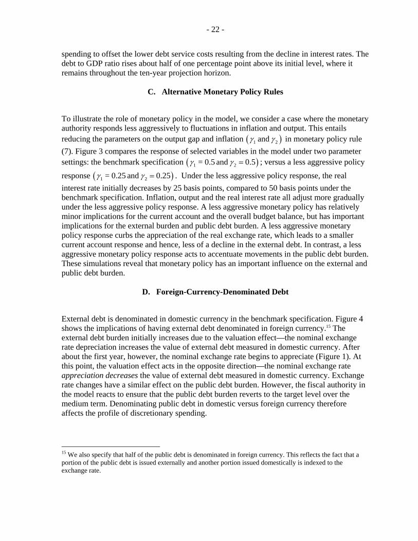
- 22 -

spending to offset the lower debt service costs resulting from the decline in interest rates. The debt to GDP ratio rises about half of one percentage point above its initial level, where it remains throughout the ten-year projection horizon.

C. Alternative Monetary Policy Rules

To illustrate the role of monetary policy in the model, we consider a case where the monetary authority responds less aggressively to fluctuations in inflation and output. This entails reducing the parameters on the output gap and inflation ( )1 2and γ γ in monetary policy rule (7). Figure 3 compares the response of selected variables in the model under two parameter settings: the benchmark specification ( )1 2= 0.5 and 0.5γ γ = ; versus a less aggressive policy

response ( )1 2= 0.25 and 0.25γ γ = . Under the less aggressive policy response, the real interest rate initially decreases by 25 basis points, compared to 50 basis points under the benchmark specification. Inflation, output and the real interest rate all adjust more gradually under the less aggressive policy response. A less aggressive monetary policy has relatively minor implications for the current account and the overall budget balance, but has important implications for the external burden and public debt burden. A less aggressive monetary policy response curbs the appreciation of the real exchange rate, which leads to a smaller current account response and hence, less of a decline in the external debt. In contrast, a less aggressive monetary policy response acts to accentuate movements in the public debt burden. These simulations reveal that monetary policy has an important influence on the external and public debt burden.

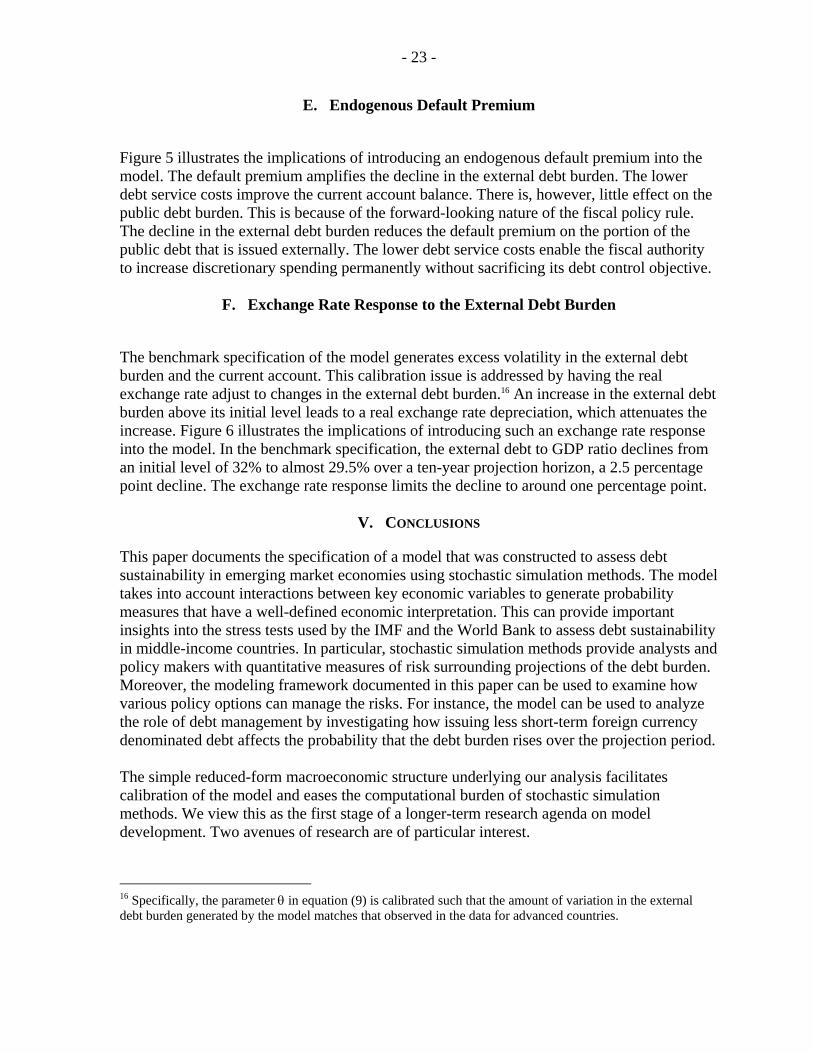
D. Foreign-Currency-Denominated Debt

External debt is denominated in domestic currency in the benchmark specification. Figure 4 shows the implications of having external debt denominated in foreign currency.15 The external debt burden initially increases due to the valuation effect—the nominal exchange rate depreciation increases the value of external debt measured in domestic currency. After about the first year, however, the nominal exchange rate begins to appreciate (Figure 1). At this point, the valuation effect acts in the opposite direction—the nominal exchange rate appreciation decreases the value of external debt measured in domestic currency. Exchange rate changes have a similar effect on the public debt burden. However, the fiscal authority in the model reacts to ensure that the public debt burden reverts to the target level over the medium term. Denominating public debt in domestic versus foreign currency therefore affects the profile of discretionary spending.

15 We also specify that half of the public debt is denominated in foreign currency. This reflects the fact that a portion of the public debt is issued externally and another portion issued domestically is indexed to the exchange rate.

- 23 -

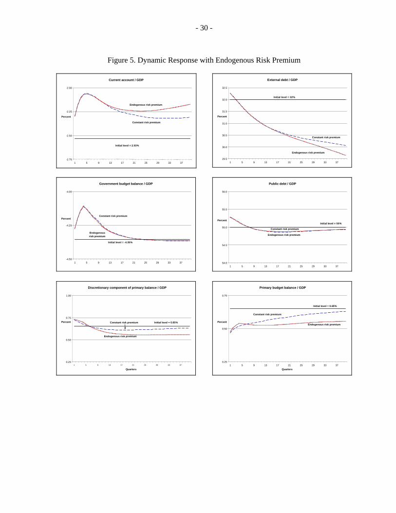
E. Endogenous Default Premium

Figure 5 illustrates the implications of introducing an endogenous default premium into the model. The default premium amplifies the decline in the external debt burden. The lower debt service costs improve the current account balance. There is, however, little effect on the public debt burden. This is because of the forward-looking nature of the fiscal policy rule. The decline in the external debt burden reduces the default premium on the portion of the public debt that is issued externally. The lower debt service costs enable the fiscal authority to increase discretionary spending permanently without sacrificing its debt control objective.

F. Exchange Rate Response to the External Debt Burden

The benchmark specification of the model generates excess volatility in the external debt burden and the current account. This calibration issue is addressed by having the real exchange rate adjust to changes in the external debt burden.16 An increase in the external debt burden above its initial level leads to a real exchange rate depreciation, which attenuates the increase. Figure 6 illustrates the implications of introducing such an exchange rate response into the model. In the benchmark specification, the external debt to GDP ratio declines from an initial level of 32% to almost 29.5% over a ten-year projection horizon, a 2.5 percentage point decline. The exchange rate response limits the decline to around one percentage point.

V. CONCLUSIONS

This paper documents the specification of a model that was constructed to assess debt sustainability in emerging market economies using stochastic simulation methods. The model takes into account interactions between key economic variables to generate probability measures that have a well-defined economic interpretation. This can provide important insights into the stress tests used by the IMF and the World Bank to assess debt sustainability in middle-income countries. In particular, stochastic simulation methods provide analysts and policy makers with quantitative measures of risk surrounding projections of the debt burden. Moreover, the modeling framework documented in this paper can be used to examine how various policy options can manage the risks. For instance, the model can be used to analyze the role of debt management by investigating how issuing less short-term foreign currency denominated debt affects the probability that the debt burden rises over the projection period. The simple reduced-form macroeconomic structure underlying our analysis facilitates calibration of the model and eases the computational burden of stochastic simulation methods. We view this as the first stage of a longer-term research agenda on model development. Two avenues of research are of particular interest.

16 Specifically, the parameter θ in equation (9) is calibrated such that the amount of variation in the external debt burden generated by the model matches that observed in the data for advanced countries.

- 24 -

First, much can be done to develop the macroeconomic structure based on more explicit microfoundations. It would be of great interest (and challenging) to develop the macro core of the model using a choice-theoretic, optimizing intertemporal framework like that underlying the Global Fiscal Model (GFM) recently developed by the IMF.17 GFM applies the rigorous microfoundations of the new open economy macroeconomics paradigm to analyze fiscal policy issues. GFM includes a fiscal and external sector but does not include some of the features outlined in the current paper that were shown to play a prominent role in assessing debt sustainability, notably a maturity structure for public and external debt, foreign- versus domestic-currency denominated debt, the pricing of traded goods and an endogenous default premium. Incorporating some of these features into a model like GFM would enable one to assess debt sustainability in the context of a more modern macroeconomic structure. Second, the specification of the model needs to be modified in order to assess debt sustainability in specific emerging market economies. The model is currently calibrated to match selected broad, stylized facts that are common across a large set of emerging market economies. In applications to specific countries, the model would need to be calibrated to match the distinctive features of individual economies. Part of the calibration exercise is quite straightforward – some aspects of the model (for instance the maturity structure of external and public debt and the portions denominated in foreign currency) can be easily modified to match the characteristics of individual economies. Other aspects of the model–such as differences in behavioral parameters–would need to be calibrated with the aid of additional empirical work and intuition. Moreover, the structure of the model needs to be kept relatively simple initially to make it easier for practitioners to apply the methods. Any extended version can be built in layers so users can more easily track the influence of added features on model properties.

17 GFM is similar in spirit to the Global Economy Model (GEM), a large-scale multi-country Dynamic Stochastic General Equilibrium (DSGE) model developed by the IMF. As the name implies GFM has a more comprehensive fiscal sector. See Botman and others (2006) for a detailed description of the model.

- 25 -

Figure 1. Dynamic Response to Adverse Aggregate Demand Shock-Benchmark Scenario

Output gap ("yc" = deviation of GDP from potential level)

-1.00

-0.75

-0.50

-0.25

0.00

1 5 9 13 17 21 25 29 33 37

Perc

ent

Real interest rates

7.00

7.25

7.50

7.75

8.00

8.25

8.50

1 5 9 13 17 21 25 29 33 37

Percent

Short term real interest rate

Implicit real interest rate on external debt

Initial level (7.5%)

Initial level (8.3%)

Exchange rate

-2.0 -1.5 -1.0 -0.5 0.0 0.5 1.0 1.5

1 5 9 13 17 21 25 29 33 37

Percent

Nominal exchange rate "s"

Real exchange rate

Inflation

3.25

3.50

3.75

4.00

4.25

1 5 9 13 17 21 25 29 33 37

Perc

ent

Quarterly inflation (at annual rate)

Initial level = 4%

External debt / GDP

30.5

31.0

31.5

32.0

32.5

1 5 9 13 17 21 25 29 33 37

Percent

External debt as a percent of GDP "edebt / ygdp" "

Initial level = 32%

External debt as a percent of potential GDP "edebt / ygdpp"

Current account / GDP

-2.8

-2.5

-2.3

-2.0

1 5 9 13 17 21 25 29 33 37

Percent

Current account balance as a percent of potential GDP "cabal /ygdpp"

Initial level = -2.53%

- 26 -

Figure 1. Dynamic Response to Adverse Aggregate Demand Shock-Benchmark Scenario (continued)

¹From this figure onward, we choose potential output (ygdpp) on the denominator to eliminate any effect coming from GDP.

Public debt / GDP¹

54.75

55.00

55.25

55.50

55.75

1 5 9 13 17 21 25 29 33 37

Percent

Public debt as a percent of potential GDP "pdebt / ygdpp"

Public debt as a percent of GDP "pdebt / ygdp"

Initial level = 55%

Government budget balance / GDP

-4.50

-4.25

-4.00

1 5 9 13 17 21 25 29 33 37

Perc

ent

Overall budget balance as a percent of potential GDP "bal / ygdpp"


Public debt service / GDP

4.50

4.75

5.00

5.25

1 5 9 13 17 21 25 29 33 37

Quarters

Percent Public debt service as a percent of potential GDP "dspd / ygdpp"

Initial level = 5.02%

Primary budget balance / GDP

0.25

0.50

0.75

1 5 9 13 17 21 25 29 33 37Quarters

Percent Primary budget balance as a percent of potential GDP "pbal / ygdpp "


Discretionary component of primary budget balance as a percent of potential GDP "pbal / ygdpp"

- 27 -

Figure 2. Dynamic Response with Alternative Fiscal Policy Rules


-4.50

-4.25

-4.00

1 5 9 13 17 21 25 29 33 37

Percent Benchmark fiscal policy rule: flexible debt target

Cyclical-adjusted budget balance target = Initial level = -4.35%

Cyclcial adjusted debt target

Public debt / GDP

54.75

55.00

55.25

55.50

55.75

1 5 9 13 17 21 25 29 33 37

Percent

Benchmark fiscal policy rule: flexible debt target

Cyclical-adjusted budget balance target

Cyclical adjusted debt target = Initial level = 55%

Discretionary component of primary balance / GDP

0.25

0.50

0.75

1.00

1 5 9 13 17 21 25 29 33 37

Quarters

Percent Benchmark fiscal policy rule: flexible debt target

Cyclical-adjusted budget balance target


Cyclical-adjusted debt target


0.25

0.50

0.75

1 5 9 13 17 21 25 29 33 37Quarters

Percent

Benchmark fiscal policy rule Cyclical-adjusted budget balance rule

Initial level = 0.65% Cyclical-adjusted

debt target

- 28 -

Figure 3. Dynamic Response with Less Aggressive Monetary Policy Rule


-2.75

-2.50

-2.25

-2.00

1 5 9 13 17 21 25 29 33 37

Percent

Benchmark monetary policy rule

Less aggressive monetary policy rule


External debt / GDP

30.5

31.0

31.5

32.0

1 5 9 13 17 21 25 29 33 37

Percent



Initial level = 32%


-4.50

-4.25

-4.00

1 5 9 13 17 21 25 29 33 37

Quarters

Percent




Short-term real interest rates

7.00

7.25

7.50

7.75

1 5 9 13 17 21 25 29 33 37

Percent




Output gap (deviation of GDP from potential level)

-1.25

-1.00

-0.75

-0.50

-0.25

0.00

1 5 9 13 17 21 25 29 33 37

Percent



Inflation

3.25

3.50

3.75

4.00

1 5 9 13 17 21 25 29 33 37

Percent



Real exchange rate

0.00

0.25

0.50

0.75

1.00

1.25

1 5 9 13 17 21 25 29 33 37

Percent



Public debt / GDP

55.00

55.25

55.50

1 5 9 13 17 21 25 29 33 37

Quarters

Percent



Initial level = 55%

- 29 -

Figure 4. Dynamic Response with Foreign-Currency-Denominated Debt


-2.75

-2.50

-2.25

-2.00

1 5 9 13 17 21 25 29 33 37

Percent External debt denominated in

domestic currency


External debt denominated in foreign currency

External debt / GDP

30.0

30.5

31.0

31.5

32.0

32.5

1 5 9 13 17 21 25 29 33 37

Percent

Initial level = 32%

External debt denominated in domestic currency



-4.50

-4.25

-4.00

1 5 9 13 17 21 25 29 33 37

Percent




Public debt / GDP

54.00

54.50

55.00

55.50

56.00

1 5 9 13 17 21 25 29 33 37

PercentInitial level = 55%




0.25

0.50

0.75

1.00

1 5 9 13 17 21 25 29 33 37

Quarters

Percent External debt denominated in domestic currency



0.25

0.50

0.75

1 5 9 13 17 21 25 29 33 37Quarters

Percent




- 30 -

Figure 5. Dynamic Response with Endogenous Risk Premium


-2.75

-2.50

-2.25

-2.00

1 5 9 13 17 21 25 29 33 37

Percent Endogenous risk premium


Constant risk premium

External debt / GDP

29.5

30.0

30.5

31.0

31.5

32.0

32.5

1 5 9 13 17 21 25 29 33 37

Percent

Initial level = 32%

Endogenous risk premium



-4.50

-4.25

-4.00

1 5 9 13 17 21 25 29 33 37

Percent




Public debt / GDP

54.0

54.5

55.0

55.5

56.0

1 5 9 13 17 21 25 29 33 37

PercentInitial level = 55%

Constant risk premium Endogenous risk premium


0.25

0.50

0.75

1.00

1 5 9 13 17 21 25 29 33 37

Quarters

Percent Constant risk premium




0.25

0.50

0.75

1 5 9 13 17 21 25 29 33 37Quarters

Percent


Constant risk premium Endogenous risk premium

- 31 -

Figure 6.Dynamic Response with Exchange Rate Response to External Debt

Real exchange rate

-0.50

0.00

0.50

1.00

1 5 9 13 17 21 25 29 33 37

Perc

ent

Exchange rate response to external debt burden


0.25

0.50

0.75

1.00

1 5 9 13 17 21 25 29 33 37

Quarters

Percent Initial level = 0.65%



0.25

0.50

0.75

1 5 9 13 17 21 25 29 33 37

Quarters

Perc

ent



Output gap (deviation of GDP from potential level)

-1.25

-1.00

-0.75

-0.50

-0.25

0.00

1 5 9 13 17 21 25 29 33 37

Perc

ent



-2.75

-2.50

-2.25

-2.00

1 5 9 13 17 21 25 29 33 37

Perc

ent



External debt / GDP

29.5

30.0

30.5

31.0

31.5

32.0

32.5

1 5 9 13 17 21 25 29 33 37

Perc

ent

Initial level = 32%



-4.50

-4.25

-4.00

1 5 9 13 17 21 25 29 33 37

Perc

ent



Public debt / GDP

54.0

54.5

55.0

55.5

56.0

1 5 9 13 17 21 25 29 33 37

Perc

ent Initial level = 55%


- 32 -

REFERENCES

Barnhill, T., and G. Kopits (2003), “Assessing Fiscal Sustainability under Uncertainty”, IMF Working Paper 03/09 (Washington: International Monetary Fund).

Bayoumi, T., D. Laxton, and P. Pesenti, 2004, “Benefits and Spillovers of Greater Competition in Europe: A Macroeconomic Assessment,” ECB Working Paper Series No. 341, April (Frankfurt, European Central Bank).

Berg, A., P. Karam, and D. Laxton, 2006, “A Practical Model-Based Approach to Monetary Policy Analysis—How-to-Guide,” IMF Working Paper 06/81 (Washington: International Monetary Fund).

Botman, D., D. Laxton, D. Muir and A. Romanov, 2006, “A New-Open-Economy-Macro Model for Fiscal Policy Evaluation,” IMF Working Paper 06/045 (Washington: International Monetary Fund).

Garcia, M., and R. Rigobon (2004), “A Risk Management Approach to Emerging Market’s Sovereign Debt Sustainability with an Application to Brazilian Data”, NBER Working Paper 10336 (March).

Hostland, D., and P. Karam, 2005, “Assessing Debt Sustainability in Emerging Market Economies Using Stochastic Simulation Methods,” IMF Working Paper WP/05/226 (Washington: International Monetary Fund).

Hostland, D., and L. Schembri, 2005, “External Adjustment and Debt Sustainability” in Exchange Rates, Capital Flows and Policy, ed. by Rebecca Driver, Peter Sinclair, and Christoph Thoenissen, Routledge International Studies in Money and Banking (Oxford: Routledge), Chapter 12, pp. 261–300.

International Monetary Fund, 2002, “Assessing Sustainability”, SM/02/06 (May 28, 2002).

———, 2003, “Sustainability Assessments – Review of Application and Methodological Refinements,” Discussion Paper, June 23 (Washington).

———, 2005, World Economic Outlook, September (Washington).

IMF and World Bank, 2004a, “Debt Sustainability in Low-Income Countries: Proposal for an Operational Framework and Policy Implications”, (February 3).

———, 2004b, “Debt Sustainability in Low-Income Countries: Further Considerations on an Operational Framework and Policy Implications”, (September 10).

Lane, P., and G.M. Milesi-Ferretti, 2005, “A Global Perspective on External Positions,” IMF Working Paper WP/05/161 (Washington: International Monetary Fund).

- 33 -

Mendoza, E., and M. Oviedo (2003), “Public Debt, Fiscal Solvency and Macroeconomic Uncertainty in Emerging Markets”, mimeo (November 2003).

Reinhart, C., K. Rogoff, and M. Savastano, 2003, “Debt Intolerance,” Brookings Papers of Economic Activity I, (The Brookings Institute, Washington), pp. 1–74.

Svensson, L., 2003, “What is Wrong with Taylor Rules? Using Judgment in Monetary Policy through Targeting Rules,” Journal of Economic Literature, Vol. 41, No. 2; p. 426 (52 pages).

Taylor, J., 1993, “Discretion Versus Policy Rules in Practice,” Carnegie-Rochester Conference Series on Public Policy 39, pp.195–214.

———, 2000, “Low Inflation, Pass-Through, and the Pricing Power of Firms,” European Economic Review, Vol. 7, No. 44, pp. 1389–408.

specification of a stochastic simulation model for ... · wp/06/268 specification of a stochastic...

Documents