Species and Functors and Types, Oh My!

Brent A. YorgeyUniversity of Pennsylvaniabyorgey@cis.upenn.edu

AbstractThe theory ofcombinatorial species, although invented as a purelymathematical formalism to unify much of combinatorics, canalsoserve as a powerful and expressive language for talking aboutdata types. With potential applications to automatic test generation,generic programming, and language design, the theory deserves tobe much better known in the functional programming community.This paper aims to teach the basic theory of combinatorial speciesusing motivation and examples from the world of functional pro-gramming. It also introduces thespecieslibrary, available on Hack-age, which is used to illustrate the concepts introduced andcanserve as a platform for continued study and research.

Categories and Subject DescriptorsD.3.3 [Language Constructsand Features]: Data types and structures; D.1.1 [ProgrammingTechniques]: Applicative (Functional) Programming; G.2.1 [Com-binatorics]

General Terms Languages, Theory

Keywords Combinatorial species, algebraic data types

1. IntroductionThe theory ofcombinatorial specieswas invented by Andre Joyalin 1981 [16] as an elegant framework for understanding and uni-fying much of enumerative combinatorics. Since then, mathemati-cians have continued to develop the theory, proving a wide rangeof fundamental results and producing at least one excellentrefer-ence text on the topic [4]. Connections to computer science andfunctional programming have been pointed out in detail, notablyby Flajolet, Salvy, and Zimmermann [12, 13]. Sadly, however, thisbeautiful theory is not widely known among functional program-mers.

Suppose Dorothy G. Programmer has created the following datatype to aid in her ethological study of alate simian family groups:

data Family a = Monkey Bool a

| Group a [Family a ]

That is, a family (parameterized by names of typea) is either asingle monkey with a boolean indicating whether it can fly, oranalpha male together with a group of families.

While developing and testing her software, Dorothy might wantto do things such as enumerate or count all the family structures of

Permission to make digital or hard copies of all or part of this work for personal orclassroom use is granted without fee provided that copies are not made or distributedfor profit or commercial advantage and that copies bear this notice and the full citationon the first page. To copy otherwise, to republish, to post on servers or to redistributeto lists, requires prior specific permission and/or a fee.

Haskell’10, September 30, 2010, Baltimore, Maryland, USA.Copyright c© 2010 ACM 978-1-4503-0252-4/10/09. . . $10.00

a certain size, or randomly generate family structures. There existtools for accomplishing at least two of these tasks: QuickCheck [9]and SmallCheck [22] can be used to do random and exhaustivegeneration, respectively.

However, suppose Dorothy now decides that the order of thefamilies in a group doesn’t matter, although she wants to continueusing the same list representation. Suddenly she is out of luck:Haskell has no way to formally describe this rather common sit-uation, and there is no easy way to inform QuickCheck and Small-Check of her intentions. She could add aBag newtype,

newtype Bag a = Bag [a ]

and endow it with custom QuickCheck and SmallCheck generators,but this is rather ad-hoc. What if she later decides that the order ofthe families does matter after all, but only up to cyclic rotations?Or that groups must always contain at least two families? Or whatif she wants to have a data structure representing the graph ofinteractions between different family groups?

What Dorothy needs is a coherent framework in which to de-scribe these sorts of sophisticated structures. The theoryof speciesis precisely such a framework: for example, her original data struc-ture can be described succinctly by theregular speciesexpressionF = 2 • X + X • (L ◦ F); Section 3 explains how to interpret thisexpression. The variants on her structure correspond tonon-regularspecies(Section 5) and can be expressed with only simple tweaks tothe original expression. The payoff is that these species expressionsform an abstract syntax (Section 6) with multiple useful semanticinterpretations, including ways to exhaustively enumerate, count,or randomly generate structures (Sections 7 and 8).

This paper is available athttp://www.cis.upenn.edu/~byorgey/papers/species-pearl.lhs as a literate Haskelldocument. Thespecieslibrary itself, together with a good dealof documentation and examples, is available on Hackage [10]athttp://hackage.haskell.org/package/species.

2. Combinatorial speciesIntuitively, a species describes afamily of structures, parameterizedby a set oflabels which identify locations in the structures. Inprogramming language terms, a species is like a polymorphictypeconstructor with a single type argument.

Definition 1. A speciesF consists of a pair of mappings,F• andF↔, with the following properties:

• F•, given a finite setU of labels, sendsU to a finite set ofstructuresF•[U ] which can be “built from” the given labels. WecallF•[U ] the set ofF-structureswith supportU , or sometimesjustF-structuresoverU .

• F↔, given a bijectionσ : U1∼

↔ U2 between two label setsU1 andU2 (i.e. a relabeling), “lifts” σ to a bijection betweenF-structures,

F↔[σ] : F•[U1]∼

↔ F•[U2].

Moreover, this lifting must befunctorial: the identity relabelingshould lift to the identity on structures, and composition ofrelabelings should commute with lifting.

We usually omit the subscript onF• when it is clear from context.

For example, Figure 1 illustrates lifting a relabelingσ to arelabeling of binary trees.

Figure 1. Relabeling a binary tree

Note that the notion ofstructuresin this definition is entirelyabstract: a “structure” is just an element of the set output by F•,which could be anything (subject to the restrictions onF).

Fans of category theory will recognize a much more conciseversion of this definition: a species is an endofunctor onB, thecategory of finite sets with bijections as arrows. You won’t need toknow any category theory to understand this paper or to make use ofthespecieslibrary; however, the categorical point of view does addconsiderable conciseness and depth to the study of combinatorialspecies.

The ability to relabel structures means that the actual labels weuse don’t matter; we get “the same structures”, up to relabeling,for any label sets of the same size. We might say that speciesareparametric in the label sets of a given size. In particular,F’saction on all label sets of sizen is determined by its action on anyparticular such set: if|U1| = |U2| and we knowF[U1], we candetermineF[U2] by lifting any bijection betweenU1 andU2. So weoften take the finite set of natural numbers{1, . . . , n} (also written[n]) asthecanonical label set of sizen, and writeF [n] for the setof F-structures built from this set.

As a final note on the definition, it is tempting to assume thatlabels play the role of the “data” held by data structures. Instead,however, labels should be thought of asnamesfor the locationswithin a structure. The idea is that data structures can be decom-posed into ashapetogether with some sort ofcontent[1, 15]. Inthis case, alabeled shapeis some sort of structure built out of la-bels, and the content can be specified by a mapping from labelstodata (which need not be injective).

3. Regular speciesAlthough the formal definition of species is good to keep in mindas a source of intuition, in practice we take an algebraic approach,building up complex species from a small set of primitive speciesand species operations. We start our tour of the species menageriewith what I term regular species.1 These should seem like oldfriends: intuitively, regular species correspond to Haskell’s alge-braic data types. We’ll step back to define regular species moreabstractly in Section 3.2, but first let’s see how to build them.

1 There is no widely accepted name for this class of species; I call themregular since they correspond to theregular tree typesof Morris et al. [20].

3.1 Basic regular species

For each primitive species or species operation, we will definea corresponding Haskell data type embodying theF• mapping—that is, values of the type will correspond toF-structures. TheF↔

mapping, in turn, can be expressed by an instance of theFunctortype class, whose methodfmap :: (a → b) → f a → f bshows how to relabel a structuref a by applying a relabelingmap a → b to each of its labels. (We can also usefmap tofill in a labeled shape with content, by applying it to a mappingfrom labels to data.) For each species we also exhibit a method toenumerate all distinct labeled structures on a given set of labels, viaan instance of theEnumerable type class shown in Figure 2. TheactualEnumerable type class used in thespecieslibrary is moresophisticated, but not fundamentally so.

class Enumerable f where

enumerate :: [a ]→ [f a ]

Figure 2. TheEnumerable type class

Finally, for each species or species operation we also exhibit apicture as an aid to intuition. These pictures are not meant to beformal, but they will generally conform to the following rules:

• The left-hand side of each picture shows a canonical set oflabels (depicted as circled numbers), either of an arbitrary size,or of a size that is “interesting” for the species being defined.Although the canonical label set[n] is used, of course the labelscould be replaced by any others.

• In the middle is an arrow labeled with the name of the speciesbeing defined.

• On the right-hand side is a set of structures, or some sort ofschematic depiction of the construction of a “typical” structure(the species then being understood to construct such structures“in all possible ways”). When the name of a species is super-imposed on a set of labels, it represents a structure of the givenspecies built from the labels.

Zero The species0 (Figure 3) corresponds to the constantly voidtype constructor. That is, it yields no structures no matterwhatlabels it is given as input. We are forced to cheat a bit in theFunctor instance for0, since Haskell does not allow empty caseexpressions.

data 0 a

instance Functor 0 where

fmap = ⊥

instance Enumerable 0 where

enumerate = [ ]

Figure 3. The primitive species0

One The species1 (Figure 4) yields a single unit structure whenapplied to an empty set of labels, and no structures otherwise.In other words, there is exactly one structure of type1 a, andit contains no locations where values of typea can be stored. It

corresponds to nullary constructors in algebraic data types. Theunit structure built by1 is shown in Figure 4 as a filled square,to emphasize the fact that it contains no labels.

data 1 a = 1

instance Functor 1 where

fmap 1 = 1

instance Enumerable 1 where

enumerate [ ] = [1]enumerate = [ ]

Figure 4. The primitive species1

The species of singletonsThe species ofsingletons,X (Figure 5),yields a single structure when applied to a singleton label set, andno structures otherwise. That is,X corresponds to the identity typeconstructor, which has exactly one way of building a structure witha single location.

data X a = X a

instance Functor X where

fmap f (X a) = X (f a)

instance Enumerable X where

enumerate [x ] = [X x ]enumerate = [ ]

Figure 5. The speciesX of singletons

Species sum We define species sum (Figure 6) to correspond totype sum,i.e.disjoint (tagged) union. Given speciesF andG and aset of labelsU , the set of(F+ G)-structures overU is the disjointunion of the sets ofF- andG-structures overU :

(F+ G)[U ] = F [U ] ⊎G[U ].

In other words, an(F + G)-structure is either anF-structure or aG-structure, along with a tag specifying which. For example,1+Xcorresponds to the familiarMaybe type constructor.

We can generalize0 and1 by defining the speciesn, for eachn > 0, to be the species which generatesn distinct structures forthe empty label set, and no structures for any nonempty labelset;n is isomorphic to1 + · · ·+ 1

︸ ︷︷ ︸

n

. For example,2 corresponds to the

constantlyBool type constructor,data CBool a = CBool Bool .It is not hard to verify that, up to isomorphism,0 is the identity

for species addition, and that+ is associative and commutative.Since these algebraic laws correspond directly to generic isomor-phisms between structures, we can represent the laws as Haskellcode. We define a type of embedding-projection pairs, shown inFigure 7. A value of typef ↔ g is an isomorphism betweenf

infixl 6 +data (f + g) a = Inl (f a) | Inr (g a)

instance (Functor f ,Functor g)⇒Functor (f + g) where

fmap h (Inl x) = Inl (fmap h x)fmap h (Inr x) = Inr (fmap h x)

instance (Enumerable f ,Enumerable g)⇒Enumerable (f + g) where

enumerate ls = map Inl (enumerate ls)++map Inr (enumerate ls)

(+) :: (f a → g a)→ (h a → j a)→ (f + h) a → (g + j ) a

(fg + hj ) (Inl fa) = Inl (fg fa)(fg + hj ) (Inr ha) = Inr (hj ha)

Figure 6. Species sum

andg , witnessed by a pair of functions, one in each direction. Wealso define the identity isomorphism as well as composition andinversion of isomorphisms.

infix 1↔data f ↔ g = (↔) {to :: ∀a. f a → g a,

from :: ∀a. g a → f a

}

ident :: f ↔ f

ident = id ↔ id

(>>>) :: (f ↔ g)→ (g ↔ h)→ (f ↔ h)(fg ↔ gf ) >>> (gh ↔ hg) = (gh ◦ fg)↔ (gf ◦ hg)

inv :: (f ↔ g)→ (g ↔ f )inv (fg ↔ gf ) = gf ↔ fg

Figure 7. Isomorphisms

Armed with these definitions, Figure 8 presents the algebraiclaws for sum in Haskell form, as implemented in thespecieslibrary. The one technical issue to note is that for the congru-encesinSumL and inSumR (and the correspondinginProdLand inProdR shown in the next section), we must be careful touse lazy pattern matches, since the isomorphism betweenf andgmay not be needed. Always forcing the proof of(f ↔ g) to weak-head normal form can cause some isomorphisms between recursivestructures (such as the one shown in Figure 15) to diverge.

Species product Just as species sum corresponds to type sum, wedefine species product (Figure 9) to correspond to type product, in

sumIdL :: 0+ f ↔ f

sumIdL = (λ(Inr x)→ x)↔ Inr

sumComm :: f + g ↔ g + f

sumComm = swapSum ↔ swapSum

where swapSum (Inl x) = Inr x

swapSum (Inr x) = Inl x

sumAssoc :: f + (g + h)↔ (f + g) + h

sumAssoc = reAssocL↔ reAssocR

where reAssocL (Inl x) = Inl (Inl x)reAssocL (Inr (Inl x)) = Inl (Inr x)reAssocL (Inr (Inr x)) = Inr x

reAssocR (Inl (Inl x)) = Inl x

reAssocR (Inl (Inr x)) = Inr (Inl x)reAssocR (Inr x) = Inr (Inr x)

inSumL :: (f ↔ g)→ (f + h ↔ g + h)inSumL ∼ (fg ↔ gf ) = (fg + id)↔ (gf + id)

inSumR :: (f ↔ g)→ (h + f ↔ h + g)inSumR ∼ (fg ↔ gf ) = (id + fg)↔ (id + gf )

Figure 8. Algebraic laws for sum

such a way that the resulting structures contain each label exactlyonce. So, to form an(F • G)-structure overU , we splitU into twodisjoint subsets, and form an ordered pair of anF-structure builtfrom the first subset and aG-structure built from the second. Doingthis in all possible ways yields the species(F • G). Formally,

(F • G)[U ] =∑

U=U1⊎U2

F[U1]× G[U2],

where∑

denotes repeated disjoint union and× denotes Cartesianproduct of sets.

infixl 7 •data (f • g) a = f a • g a

instance (Functor f ,Functor g)⇒Functor (f • g) where

fmap h (x • y) = fmap h x • fmap h y

instance (Enumerable f ,Enumerable g)⇒Enumerable (f • g) where

enumerate ls = [x • y | (fls, gls)← splits ls

, x ← enumerate fls

, y ← enumerate gls ]

splits :: [a ]→ [([a ], [a ])]splits [ ] = [([ ], [ ])]splits (x : xs) = (map ◦ first) (x :) ss

++ (map ◦ second) (x :) sswhere ss = splits xs

first f (x , y) = (f x , y)second f (x , y) = (x , f y)

Figure 9. Species product

For example,X•X (which can be abbreviatedX2) is the speciesof ordered pairs. X yields no structures unless it is given a singlelabel, so the only way to get anX • X structure is if we start withtwo labels and partition them into two singleton sets to passonto theX’s. Of course, there are two ways to do this, reflecting thetwo possible orderings of the labels. Similarly,X3 is the species ofordered triples, with3! = 6 orderings for the labels, and so on.

Up to isomorphism,1 is an identity for species product, and0is an annihilator. It is also not hard to check that• is associativeand commutative, and distributes over+ (as usual, all up to iso-morphism). Thus, species form a commutative semiring. The iso-morphisms justifying these algebraic laws are shown in Figure 10,although their straightforward implementations are omitted in theinterest of space.

prodIdL :: 1 • f ↔ f

prodIdR :: f • 1↔ f

prodAbsorbL :: 0 • f ↔ 0

prodComm :: f • g ↔ g • fprodAssoc :: f • (g • h)↔ (f • g) • hprodDistrib :: f • (g + h)↔ (f • g) + (f • h)

inProdL :: (f ↔ g)→ (f • h ↔ g • h)inProdR :: (f ↔ g)→ (h • f ↔ h • g)

Figure 10. Algebraic laws for product

Least fixed points and the implicit species theoremIf we adda least fixed point operatorµ, we now get theregular typesoralgebraic data typesfamiliar to any functional programmer [20].For example, the speciesL of linear orderings(or lists for short)can be defined as

L = µℓ.1+ X • ℓ.

That is, a list is either empty (1) or an element paired with a list(X•ℓ). For any setU of labels,L[U ] is the set of all linear orderingsof U (Figure 11); of course,|L[n]| = n!.

instance Enumerable [ ] where

enumerate = Data .List .permutations

listRec :: [ ]↔ 1+ (X • [ ])listRec = unroll ↔ roll

where unroll [ ] = Inl 1

unroll (x : xs) = Inr (X x • xs)roll (Inl 1) = [ ]roll (Inr (X x • xs)) = x : xs

Figure 11. The speciesL of linear orderings

Actually, mathematicians would not writeL = µℓ.1+X• ℓ, butsimply

L = 1+ X • L.

This is not because they are being sloppy, but because of theimplicit species theorem[4], which is a combinatorial analogue ofthe implicit function theorem from analysis. Suppose we have aspecies equation which implicitly definesF in terms of itself. If

F yields no structures on the empty label set, and is not triviallyreducible to itself, then the implicit species theorem guarantees thatthere is a unique solution forF with F(0) = 0, which is exactly theleast fixed point of the implicit equation. Of course, the criteriagiven above are somewhat vague; a more precise formulation isexplained in Section 8.1.

The speciesL, as defined above, does not actually meet thesecriteria, since it yields a structure on the empty label set.However,if we letL+ denote the species of nonempty lists, withL++1 = L,then we haveL+ = X • (L+ + 1), which does meet the criteriaand hence has a unique solution. Thus,L = 1 + L+ is uniquelydetermined as well, and we are justified in forgetting aboutµ andsimply manipulating the implicit equationL = 1+X • L howeverwe like. For example, expandingL in its own definition, we findthat

L = 1+ X • L

= 1+ X • (1+ X • L)

= 1+ X+ X2 • L

Continuing this process, we find thatL = 1+X+X2 +X3 + . . . ,which corresponds to the observation that a list is either empty, ora single element, or an ordered pair, or an ordered triple, and so on.We can also “solve” the implicit equation forL to obtainL = 1

1−X.

This may seem nonsensical at this point—we have defined neithersubtraction nor division of species—but it is perfectly valid in thecontext of virtual species (Section 8.1), and directly corresponds tothe exponential generating function forL (Section 7).

As another example of recursive species and the power of theimplicit species theorem, consider the Haskell data types shown inFigure 12.

data BTree a = Empty

| Node a (BTree a) (BTree a)

data Paren a = Leaf a

| Pair (Paren a) (Paren a)

Figure 12. Binary trees and binary parenthesizations

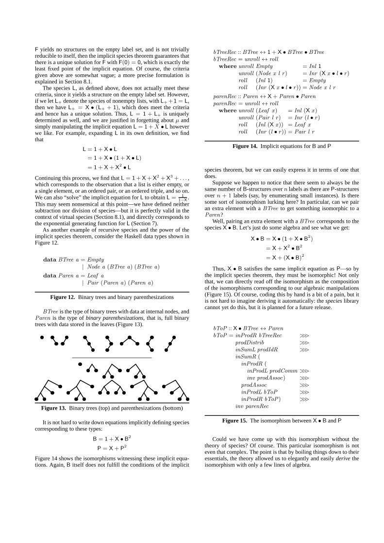
BTree is the type of binary trees with data at internal nodes, andParen is the type ofbinary parenthesizations, that is, full binarytrees with data stored in the leaves (Figure 13).

Figure 13. Binary trees (top) and parenthesizations (bottom)

It is not hard to write down equations implicitly defining speciescorresponding to these types:

B = 1+ X • B2

P = X+ P2

Figure 14 shows the isomorphisms witnessing these implicitequa-tions. Again,B itself does not fulfill the conditions of the implicit

bTreeRec :: BTree ↔ 1+ X • BTree • BTreebTreeRec = unroll ↔ roll

where unroll Empty = Inl 1

unroll (Node x l r) = Inr (X x • l • r)roll (Inl 1) = Empty

roll (Inr (X x • l • r)) = Node x l r

parenRec :: Paren ↔ X+ Paren • ParenparenRec = unroll ↔ roll

where unroll (Leaf x) = Inl (X x)unroll (Pair l r) = Inr (l • r)roll (Inl (X x)) = Leaf x

roll (Inr (l • r)) = Pair l r

Figure 14. Implicit equations forB andP

species theorem, but we can easily express it in terms of one thatdoes.

Suppose we happen to notice that there seem to always be thesame number ofB-structures overn labels as there areP-structuresovern + 1 labels (say, by enumerating small instances). Is theresome sort of isomorphism lurking here? In particular, can wepairan extra element with aBTree to get something isomorphic to aParen?

Well, pairing an extra element with aBTree corresponds to thespeciesX • B. Let’s just do some algebra and see what we get:

X • B = X • (1+ X • B2)

= X+ X2 • B2

= X+ (X • B)2

Thus,X • B satisfies the same implicit equation asP—so bythe implicit species theorem, they must be isomorphic! Not onlythat, we can directly read off the isomorphism as the compositionof the isomorphisms corresponding to our algebraic manipulations(Figure 15). Of course, coding this by hand is a bit of a pain, but itis not hard to imagine deriving it automatically: thespecieslibrarycannot yet do this, but it is planned for a future release.

bToP :: X • BTree ↔ Paren

bToP = inProdR bTreeRec >>>prodDistrib >>>inSumL prodIdR >>>inSumR (

inProdR (inProdL prodComm >>>inv prodAssoc) >>>

prodAssoc >>>inProdL bToP >>>inProdR bToP) >>>

inv parenRec

Figure 15. The isomorphism betweenX • B andP

Could we have come up with this isomorphism without thetheory of species? Of course. This particular isomorphism is noteven that complex. The point is that by boiling things down totheiressentials, the theory allowed us to elegantly and easilyderivetheisomorphism with only a few lines of algebra.

3.2 Regular species, formally

We are now ready to state the precise definition of regular species.A first characterization is as follows:

Definition 2. A speciesF is regular if it can be expressed in termsof 1, X, +, •, and least fixed point.

This definition validates the promised intuition that regularspecies correspond to Haskell algebraic data types, since normalHaskell98 data type declarations provide exactly these features(forgetting for the moment about infinite data structures).

However, there is a more direct characterization that makesapparent why this particular collection of species is interesting. Wemust first define what we mean by thesymmetriesof a structure.Recall thatSn denotes the termsymmetric group of ordern, whichhaspermutationsof sizen (that is, bijections between{1, . . . , n}and itself) as elements, and composition of permutations asthegroup operation.

Definition 3. A permutation σ ∈ Sn is a symmetryof anF-structuref ∈ F[U ] if and only if σ fixesf , that is,F↔[σ](f) =f .

For example, Figure 16 depicts a tree with a set of labels at eachnode. This structure has many nontrivial symmetries, such as thepermutation which swaps4 and 6 but leaves all the other labelsunchanged; since4 and6 are in the same set, swapping them hasno effect.

Figure 16. A labeled structure with nontrivial symmetries

However, the binary trees shown in Figure 1 have only the trivialsymmetry, since permuting their labels in any nontrivial way yieldsdifferent trees.

Definition 4. A speciesF is regular if every F-structure has theidentity permutation as its only symmetry; such structuresare alsocalled regular.

It turns out that these two definitions are equivalent (with theslight caveat that we must allow countably infinite sums and prod-ucts in the first definition). That species built from sum, product,and fixed point have no symmetries is not hard to see; less obviousis the fact that up to isomorphism, every species with no symme-tries can be expressed in this way (a proof sketch is given in Sec-tion 8.1). Of course, since we cannot write down infinite sumsorproducts in Haskell, there are some regular species which cannot beexpressed as simple algebraic data types. For example, the regularspecies of prime-length lists,

X2 + X

3 + X5 + X

7 + X11 + . . . ,

cannot be written as a simple algebraic data type.2 But aside frominfinite sums and products, as long as we stick to data structures

2 Although I am sure it can be expressed using GADTs and type-levelarithmetic. . .

with no symmetries, Haskell’s data types are perfectly adequate toexpress any data structure we could possibly think up.

3.3 Other operations on regular species

In addition to sum and product, the class of regular species is alsoclosed under other fundamental operations.

Species composition Given speciesF andG, thecompositionF ◦G is a species which builds “F-structures made out ofG-structures”,with the underlying labels distributed to theG-structures so thateach label occurs exactly once in the overall structure (Figure 17).However, in order to ensure we get only a finite number of(F ◦G)-structures of each size,G must not yield any structures on the emptylabel set. This corresponds exactly to the criterion for composingformal power series, namely, that the inner series have no constantterm.

Specifically, to build an(F ◦G)-structure over a label setU , we

• partitionU into some number of nonempty disjoint parts,U =U1 ⊎ U2 ⊎ · · · ⊎ Uk;

• create aG-structure on each of theUi;

• create anF-structure on theseG-structures.

Doing this in all possible ways yields the set of(F ◦ G)-structuresoverU .

newtype (f ◦ g) a = C {unC :: f (g a)}

instance (Functor f ,Functor g)⇒Functor (f ◦ g) where

fmap h = C ◦ (fmap ◦ fmap) h ◦ unC

instance (Enumerable f ,Enumerable g)⇒Enumerable (f ◦ g) where

enumerate ls =[C y | p ← partitions ls

, gs ← mapM enumerate p

, y ← enumerate gs ]

partitions :: [a ]→ [[[a ]]]partitions [ ] = [[ ]]partitions (x : xs) = [ (x : ys) : p

| (ys, zs)← splits xs

, p ← partitions zs

]

Figure 17. Species composition

For example,R = X • (L ◦ R) (whereL denotes the speciesof linear orderings) defines the species ofrose trees, as definedin Data.Tree, with each node having a data element and anynumber of children. We can also easily encodenested data types[6] (such types are sometimes called “non-regular”, although thatnomenclature is confusing in the current context, since they do infact correspond to regular species). For example,B = X+B◦X2 isthe species ofcomplete binary trees; aB-structure is either a singleleaf, or a complete binary tree withpairs of elements at the leaves.

It is not hard to verify that composition is associative (butnotcommutative), and that it hasX as both a left and right identity.Composition also distributes over both sum and product fromtheright: (F+G)◦H = (F◦H)+(G◦H), and similarly for(F•G)◦H.

As noted at the beginning of this section, regular species areclosed under composition. Although we won’t prove this formally,it makes intuitive sense: if anF-structure has no symmetries, andin each location we put aG-structure which also has no symme-tries, the resulting composed structure cannot have any symmetrieseither.

Differentiation Of course, no discussion of an algebra for datatypes would be complete without mentioning differentiation. Therehas been a great deal of fascinating work in the functional program-ming community on differentiating data structures [2, 14, 17, 18].As usual, however, the mathematicians beat us to it!

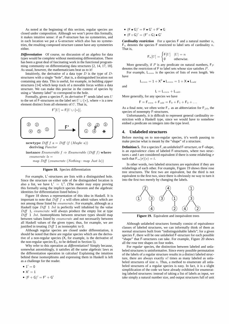
Intuitively, the derivative of a data typeD is the type ofD-structures with a single “hole”, that is, a distinguished location notcontaining any data. This is useful, for example, in building zipperstructures [14] which keep track of a movable focus within a datastructure. We can make this precise in the context of speciesbyusing a “dummy label” to correspond to the hole.

Formally, given a speciesF, its derivativeF′ sends label setsUto the set ofF-structures on the label setU ∪{∗}, where∗ is a newelement distinct from all elements ofU . That is,

F′[U ] = F[U ∪ {∗}].

newtype Diff f a = Diff (f (Maybe a))deriving Functor

instance Enumerable f ⇒ Enumerable (Diff f ) where

enumerate ls =map Diff (enumerate (Nothing :map Just ls))

Figure 18. Species differentiation

For example,L′-structures are lists with a distinguished hole.Since the structure on either side of the distinguished location isalso a list, we haveL′ = L2. (The reader may enjoy provingthis formally using the implicit species theorem and the algebraicidentities for differentiation listed below.)

Figure 18 shows a representation of this idea in Haskell. It isimportant to note thatDiff f a will often admit values which arenot among those listed byenumerate . For example, although as aHaskell typeDiff 1 Int is perfectly well inhabited by the valueDiff 1, enumerate will always produce the empty list at typeDiff 1 Int . Isomorphisms between structure types should mapbetween values listed byenumerate and not necessarily betweenall Haskell values of the given types; thus, for example, we arejustified in treatingDiff 1 as isomorphic to0.

Although regular species are closed under differentiation, itshould be noted that there are regular species which are the deriva-tive of a non-regular species (X, for example, is the derivative ofthe non-regular speciesE2, to be defined in Section 5).

Why refer to this operation asdifferentiation? Simply because,somewhat astonishingly, it satisfies all the same algebraiclaws asthe differentiation operation in calculus! Explaining theintuitionbehind these isomorphisms and expressing them in Haskell isleftas a challenge for the reader.

• 1′ = 0

• X′ = 1

• (F+ G)′ = F′ + G′

• (F • G)′ = F • G′ + F′ • G

• (F ◦ G)′ = (F′ ◦ G) • G′

Cardinality restriction For a speciesF and a natural numbern,Fn denotes the speciesF restricted to label sets of cardinalityn.That is,

Fn[U ] =

{

F[U ] |U | = n

∅ otherwise.

More generally, ifP is any predicate on natural numbers,FP

denotes the restriction ofF to label sets whose size satisfiesP .For example,Leven is the species of lists of even length. We

have

Leven = 1+ X2 • Leven = 1+ X • Lodd

and

L = Leven + Lodd .

More generally, for any species we have

F = Feven + Fodd = F0 + F1 + F2 + . . .

As a final note, we often writeF+ as an abbreviation forF>0, thespecies of nonemptyF-structures.

Unfortunately, it is difficult to represent general cardinality re-striction with a Haskell type, since we would have to somehowembed a predicate on integers into the type level.

4. Unlabeled structuresBefore moving on to non-regular species, it’s worth pausingtomake precise what is meant by the “shape” of a structure.

Definition 5. For a speciesF, anunlabeledF-structure, orF-shape,is an equivalence classof labeledF-structures, where two struc-turess andt are considered equivalent if there is some relabelingσsuch thatF↔[σ](s) = t.

In other words, two labeled structures are equivalent if they arerelabelings of each other. For example, Figure 19 shows three rosetree structures. The first two are equivalent, but the third is notequivalent to the first two, since there is obviously no way toturn itinto the first two merely by changing the labels.

Figure 19. Equivalent and inequivalent trees

Although unlabeled structures formally consist of equivalenceclasses of labeled structures, we can informally think of them asnormal structures built from “indistinguishable labels”;for a givenspeciesF, there will be one unlabeledF-structure for each possible“shape” thatF-structures can take. For example, Figure 20 showsall the rose tree shapes on four nodes.

For regular species, the distinction between labeled and unla-beled structures is uninformative. Since every possible permutationof the labels of a regular structure results in a distinct labeled struc-ture, there are always exactlyn! times as many labeled as unla-beled structures of sizen. Thus, a method to enumerate all unla-beled structures of a regular species is easy. In fact, it is aslightsimplification of the code we have already exhibited for enumerat-ing labeled structures: instead of taking a list of labels asinput, wetake simply a natural number size, and output structures full of unit

Figure 20. Unlabeled rose trees of size4

values. Enumerating unlabeled structures fornon-regularspecies,however, is much more complicated; a partial implementation ofunlabeled enumeration can be found in thespeciespackage. Forexample, we can enumerate all unlabeled sets of sets of size4, cor-responding to integer partitions of4:

> enumerateU (set ‘o‘ nonEmpty set) 4:: [Comp Set Set ()]

[{{(),(),(),()}},{{(),()},{(),()}},{{()},{(),(),()}},{{()},{()},{(),()}},{{()},{()},{()},{()}}]

5. Beyond regular speciesAs promised, the theory of combinatorial species can describestructures with nontrivial symmetries just as easily as regular struc-tures. This section introduces common non-regular speciesandcombinators.

The species of setsThe primitive species ofsets, usually denotedE (from the Frenchensemble), represents unordered collectionsof elements. For any given set of labels, there is exactly onesetstructure, the set of labels itself. It is easy to see thatE is not regular,sinceE-structures have every possible symmetry; permuting theelements of a set leaves the set unchanged.

Although the standard mathematical name for this species isthe species ofsets, a better name for it from a computer scienceperspective is the species ofbags. The termset usually indicatesboth that the order of the elements doesn’t matter and that thereare no duplicate elements; the species of bags only embodiestheformer, since we can have non-injective mappings from labels todata. However, to model sets we can certainly restrict ourselves toinjective mappings.

newtype Bag a = Bag [a ]deriving Functor

instance Eq a ⇒ Eq (Bag a) where

Bag xs ≡ Bag ys = xs ‘subBag ‘ ys ∧ ys ‘subBag ‘ xswhere subBag b = null ◦ foldl ′ (flip delete) b

instance Enumerable Bag where

enumerate ls = [Bag ls ]

Figure 21. The speciesE of sets

In Figure 21, we declare a Haskell data type forE by declaringBag to be isomorphic to[ ] via anewtype declaration, and de-riving a Functor instance forBag from the existing instance forlists, using GHC’snewtype derivingextension. Since we don’t care

about the order of the elements in aBag , we create anEq instanceto identify any twoBags with the same elements.

We can also useE to build other interesting and useful species.For example:

• X • E is the species ofpointed sets, also known as the speciesof elementsand sometimes writtenε. Pointed set structuresconsist of a single distinguished label paired with a set structureon the rest of the labels. Thus, there are preciselyn labeledε-structures on a set ofn labels, one for each choice of thedistinguished label.

We can also think of an(X •E) structure as consistingsolelyofthe distinguished label, since the set of remaining labels adds noinformation. In other words, we can treatE as a sort of “sink”for the elements we don’t care about, and the same techniquecan be used generally for describing structures containingonlya subset of the labels.

• E•E is the species ofsubsets, sometimes abbreviated℘ in refer-ence to the power set operator. Again,℘-structures technicallyconsist of a subset of the labels paired with its complement,butwe may (and often do) ignore the complement.

• (E ◦ E+) is the species ofset partitions: its structures arecollections of nonempty sets.

The species of cyclesThe primitive speciesC of directed cycles(Figure 22) yields all directed cyclic orderings (known in the math-ematical literature asnecklaces) of the given labels. By convention,cycles are always nonempty, and are read clockwise when repre-sented pictorially.

newtype Cycle a = Cycle [a ]deriving Functor

instance Eq a ⇒ Eq (Cycle a) where

Cycle xs ≡ Cycle ys = any (≡ ys) (rotations xs)where rotations xs = zipWith (++) (tails xs)

(inits xs)

instance Enumerable Cycle where

enumerate [ ] = [ ]enumerate (x : xs)

= (map (Cycle ◦ (x :)) ◦ permutations) xs

Figure 22. The speciesC of cycles

C is also non-regular, since each labeledC-structure is fixedby certain nontrivial permutations, namely, the ones whichonly“rotate” the labels.

An example of an interesting species we can build usingC isE◦C, the species ofpermutations, corresponding to the observationthat every permutation can be decomposed into a collection ofdisjoint cycles.

We note also that a cycle with a hole in it is isomorphic to a list,that is,C′ = L (Figure 23).

Cartesian product Given two speciesF andG, we may define theCartesian productF× G by

(F× G)[U ] = F[U ]× G[U ],

Figure 23. Differentiating a cycle

where the× on the right denotes the standard Cartesian product ofsets. That is, an(F × G)-structure is a pair of anF-structure and aG-structure, both of which are built overall the labels, instead ofpartitioning the labels as with normal product (Figure 24).How-ever, instead of thinking of the labels as being duplicated,we thinkof an (F × G)-structure as two structures which aresuperimposedon the same label set. In particular, when specifying the content foran(F×G)-structure, we should still only map each label to a singlepiece of data.

data (f × g) a = f a × g a

instance (Functor f ,Functor g)⇒Functor (f × g) where

fmap f (x × y) = fmap f x × fmap f y

instance (Enumerable f ,Enumerable g)⇒Enumerable (f × g) where

enumerate ls = [x × y | x ← enumerate ls

, y ← enumerate ls ]

Figure 24. Cartesian product of species

One interesting use of Cartesian product is to model some typeclass-polymorphic data structures, where the type class methodsprovide us with a second observable structure on the data elements.For example, a type constructorF with an Eq constraint on itsargument can be modeled by the species

F× (E ◦ E+).

Structures of this species consist of anF-structure with a super-imposed partition on the labels, with each part corresponding toan equivalence class. For example, Figure 25 shows a binary treeshape with a superimposed partition indicating which sets of el-ements are equal. Likewise, we can model anOrd constraint bysuperimposing an(L ◦ E+)-structure, which additionally places anobservable ordering on the equivalence classes.

This works particularly well in conjunction with the approachof Bernardyet al.[5] for testing polymorphic functions. Because ofparametricity, it suffices to test polymorphic functions onrandomlygenerated shapes filled withcarefully chosendata; if the functionworks correctly for the chosen data then by parametricity itwillwork correctly for any data. The above discussion shows thatwecan treatEq andOrd constraints as part of the shape of an inputstructure, and choose data to match.

Cartesian product hasE as both a left and right identity, and isassociative, commutative, and distributes over species sum. Again,implementing these laws as isomorphisms is left as an exercise forthe reader.

Functor composition The final species operation we will exploreis functor composition. Given speciesF and G, we define their

Figure 25. A (B× (E ◦ E+))-shape

functorial composite by

(F� G)[U ] = F[G[U ]],

that is, F-structures overthe set of allG-structureson U (Fig-ure 26). Like(F ◦ G)-structures, an(F � G)-structure is anF-structure ofG-structures, but instead of partitioning the labelsUamong theG-structures, we give all the labels to everyG-structure.As with Cartesian product structures,(F � G)-structures appear tocontain each label multiple times, but in fact we should still thinkof them as containing each label once, with a rich structure super-imposed on it.

data (f � g) a = FC {unFC :: f (g a)}

instance (Functor f ,Functor g)⇒Functor (f � g) where

fmap h = FC ◦ (fmap ◦ fmap) h ◦ unFC

instance (Enumerable f ,Enumerable g)⇒Enumerable (f � g) where

enumerate = map FC ◦ enumerate ◦ enumerate

Figure 26. Functor composition

The functor composition operation is especially useful fordefin-ing species of graphs and relations. For example, recallingthat℘ = E • E is the species of subsets andE2 is the species of setsrestricted to sets of size two,

℘� (E2 • E)

defines the species of simple graphs. An(E2 • E)-structure is a setof two labels, which we can think of as an undirected edge, andasimple graph is a subset of the set of all possible edges.

In fact, many graph-like species can be defined as℘ � G for asuitable speciesG. For example,G = X2 • E gives directed graphswithout self-loops, andG = ε × ε gives directed graphs with self-loops allowed (recalling thatε = X • E is the species of elements).The reader may enjoy discovering how to represent the species ofundirected graphs with self-loops allowed.

6. An embedded language of speciesWe have defined a type corresponding to each primitive species andspecies operation, but we would also like to be able to write down

and compute with species expressions at the term level. The per-fect way to do this is with atype classdefining a domain-specificlanguage of species expressions. The expressions can then be in-terpreted in different ways (for example, as exponential generatingfunctions, cycle index series, abstract syntax trees, or random gen-eration routines) depending on the types at which they are instanti-ated.

The basicSpecies type class, as defined in thespecieslibrary,is shown in Figure 27. The actualSpecies class contains additionalmethods, but this is the core essence.

class (Differential .C s)⇒ Species s where

singleton :: sset :: scycle :: s(◦) :: s → s → s

(×) :: s → s → s

(�) :: s → s → s

ofSize :: s → (Z→ Bool)→ s

Figure 27. TheSpecies type class

Some things may seem to be missing (0, 1, sum and product,differentiation) but these are actually provided by theDifferential .Cconstraint (from thenumeric-preludepackage), which ensures thatspecies are a differentiable ring. The remainder of the class requiresprimitive singleton, set, and cycle species; composition(◦), carte-sian product(×), and functor composition(�) operations; and acardinality-restricting operatorofSize.

It is not hard to put together theEnumerable instances we havealready seen into code which enumerates all the labeled structuresof a given species. The user can then call theenumerate methodon an expression of typeSpecies s ⇒ s, along with some labels touse:

-- cycles of lists> enumerate (cycle ‘o‘ (nonEmpty linOrd)) "abc"

:: [Comp Cycle [] Char][<"cba">,<"cab">,<"bca">,<"bac">,<"acb">,<"abc">,<"a","cb">,<"a","bc">,<"ca","b">,<"ac","b">,<"ba","c">,<"ab","c">,<"b","a","c">,<"a","b","c">]

-- simple graphs on three vertices> enumerate (subset @@ ksubset 2) [1,2,3]

:: [Comp Set Set Int][{},{{1,2}},{{1,3}},{{1,3},{1,2}},{{2,3}},{{2,3},{1,2}},{{2,3},{1,3}},{{2,3},{1,3},{1,2}}]

Since thespecieslibrary is able to automatically generateSpeciesexpressions representing any user-defined data type, we canalsoenumerate values of user-defined data types, such asFamily Int :

> enumerate family [1,2] :: [Family Int][ Group 2 [Group 1 []], Group 2 [Monkey True 1], Group 2 [Monkey False 1], Group 1 [Group 2 []], Group 1 [Monkey True 2], Group 1 [Monkey False 2]]

We can also control how the enumeration happens by explicitlyspecifying the species to use for theFamily type, rather than usingthe default.

7. Generating functions and countingWhat else can we do with combinatorial species? A key elementof the story we haven’t seen yet is the correspondence betweenspecies andgenerating functions. Generating functions are an in-dispensable tool in combinatorics, and have a well-developed the-ory [23]. Much of their power lies in the surprising fact thatmanynaturalpower seriesoperations (addition, multiplication, substitu-tion. . . ) have naturalcombinatorialinterpretations (disjoint union,independent choice, partition. . . ). Every species can be associatedwith several different generating functions, each of whichencodescertain aggregate information about the species.

For example, we can associate to each speciesF anexponentialgenerating function(egf) of the form

F(x) =∑

n>0

fnxn

n!,

wherefn is the number of distinct labeledF-structures of sizen.(Note thatx is a purely formal parameter, and we need not concernourselves with convergence; for a more detailed explanation ofgenerating functions, see Wilf [23].) Thus we have, for example,

• 0(x) = 0

0!x0 + 0

1!x1 + · · · = 0,

• 1(x) = 1,

• X(x) = x,

• L(x) =∑

n>0

n!

n!xn =

1

1− x,

• E(x) =∑

n>0

1

n!xn = ex,

• C(x) =∑

n>1

(n− 1)!

n!xn = − log(1− x).

(Here is another good reason to call the species of setsE!) Atfirst glance this may seem arbitrary, but quite the opposite is true:species sum, product, composition, and differentiation correspondprecisely to the same operations on formal power series! Forex-ample, ifF(x) andG(x) count the number of labeledF- andG-structures as defined above, it is easy to see thatF(x)+G(x) countsthe number of labeled(F+G)-structures in the same way, since ev-ery(F+G)-structure is either anF-structure or aG-structure (with atag). And although it is not as immediately apparent, we can verifythatF(x)G(x) = (F • G)(x) as well:

F(x)G(x) =

(∑

n>0

fnxn

n!

)(∑

n>0

gnxn

n!

)

=∑

n>0

n∑

k=0

(

fkxk

k!

)(

gn−k

xn−k

(n− k)!

)

=∑

n>0

n∑

k=0

fkgn−k

xn

k!(n− k)!

=∑

n>0

(n∑

k=0

(

n

k

)

fkgn−k

)

xn

n!

The expression in the outermost parentheses is precisely the num-ber of labeled(F • G)-structures on a label set of sizen: for eachk from 0 to n, there are

(n

k

)ways to pickk of then labels to put

in theF-structure,fk ways to create anF-structure from them, andgn−k ways to create aG-structure from the remaining labels.

The reader may also enjoy working out why species differentia-tion corresponds to exponential generating function differentiation.Seeing the correspondence between species composition andegf

substitution takes more work; the interested reader shouldlook upFaa di Bruno’s formula. There are also generating function opera-tions corresponding to Cartesian product and functor composition.Although they are not as natural as the other operations, they aresimple to define and easy to compute.

As a result, we can count labeled structures by interpretingspecies expressions as exponential generating functions,conve-niently represented by infinite lazy lists of coefficients. In fact,this particular technique of counting labeled structures has beenknown in the functional programming community for some time[19, 21]. Thespecieslibrary defines anEGF type with an appro-priateSpecies instance, and alabeled function to extract the coef-ficients from an egf. For example:

> take 10 . labeled $ 3 + x*x[3,0,2,0,0,0,0,0,0,0]

> take 10 . labeled$ cycle ‘o‘ (nonEmpty linOrd)

[0,1,3,14,90,744,7560,91440,1285200,20603520]

Thus, there are noC ◦ L+ structures of size0, one with a singlelabel, three with two labels,14 of size three, and so on. The librarycan even compute generating functions for some recursivelyde-fined species, using a quadratically converging combinatorial ana-logue of the Newton-Raphson method. For example, once Dorothyhas used thespecieslibrary to derive all the appropriate instancesfor herFamily type via Template Haskell, she can use thelabeledfunction to count them:

> take 10 . labeled $ family[0,3,6,72,1368,36000,1213920,49956480,2427788160,136075645440]

To each species we can also associate anordinary generatingfunction (ogf) and acycle index series; the first counts unlabeledstructures (shapes), and the second is a generalization of bothexponential and ordinary generating functions which also keepstrack of symmetries. There is not space to describe them here, butmore information can be found in Bergeronet al. [4] or in thedocumentation for thespecieslibrary, which includes facilities forcomputing with all three types of generating functions.

8. Extensions and applicationsIt should come as no surprise that we have barely scratched the sur-face; the theory of combinatorial species is both rich and deep. Inclosing, we will look at some extensions to the theory discussedhere which may lead to a deeper understanding of functional pro-gramming and data types, as well as potential applications of thetheory. At the time of writing, thespecieslibrary does not includesupport for any of these extensions, but their inclusion is plannedfor future releases.

8.1 Extensions

Weighted species Assigningweightsto the structures built by aspecies allows us to count and enumerate structures in much morerefined ways. For example, we can define the species of binarytrees, weighted by the number of leaves, and then easily count orenumerate only those trees with a certain number of leaves.

Multisort species We have only considered species which mapa single set of labels to a set of structures, corresponding to typeconstructors of a single argument. However, all of the theory gen-eralizes straightforwardly tomultisort species, which build struc-tures from multiple sets of labels (sorts). For example, multisort

species are exactly what we need to make the implicit speciesthe-orem precise. First, we can write an implicit equation forF in theform F = H(X,F), whereH is a two-sort species. For example, ifH(X,Y) = 1 + X • Y thenL = H(X, L) is the implicit equationdefining the species of lists. Now the necessary conditions for theimplicit species theorem to apply can now be stated precisely:

• H(0, 0) = 0 (no structures on the empty label set)

•∂H

∂Y(0, 0) = 0 (F does not trivially reduce to itself)

Extending thespecieslibrary to handle general multisort speciespresents an interesting challenge, due to Haskell’s lack ofkindpolymorphism, and is a topic for further research.

Virtual species It is possible to complete the semiring of speciesto a ring in a way analogous to the set-theoretic completion of thenatural numbers to the integers. We consider pairs of species(F,G)whereF is considered “positive” andG “negative”; more precisely,we define an equivalence relation on pairs of species such that(F,G) ∼ (H,K) if and only if F + K is isomorphic toG + H,and define virtual species as the equivalence classes of thisrela-tion. Virtual species allow us to define a multiplicative inverse forthe speciesE of sets, and from there to define multiplicative andcompositional inverses for other suitable species, solve differentialequations, and define acombinatorial logarithmwhich generalizesthe notion of structures built from connected components. Virtualspecies allow us to give a sensible and consistent meaning toequa-tions likeL = 1/(1− X).

Molecular species

Definition 6. A speciesF is molecular if all F-structures areisomorphic (i.e. relabelings of one another).

For example, the speciesX2 of ordered pairs is molecular, sincewe can go from any ordered pair to any other by relabeling. Onthe other hand, the speciesL of linear orderings is not molecular,since any two list structures of different lengths are fundamentallynon-isomorphic. We have the following three beautiful facts:

• The molecular species are precisely those that cannot be de-composed as the sum of two nonzero species.

• Every molecular species is equivalent toXn “quotiented bysome symmetries”; in particular, the molecular species of sizen are in one-to-one correspondence with the conjugacy classesof subgroups ofSn. This gives us a way to completely clas-sify molecular species and to compute with them directly. Forexample, there are four conjugacy classes of subgroups ofS3,each representing a different symmetry on three locations:thetrivial subgroup corresponds toX3 itself (no symmetry); swap-ping two locations yieldsX •E2; cycling the locations yields toC3; and identifying all the locations yieldsE3.

• Every species can be written uniquely (up to isomorphism andreordering of terms) as a sum of molecular species. This, com-bined with the previous fact, immediately gives us a completeclassification of all combinatorial species. It also provides amethod for finding canonical representatives of virtual species:given a pair(F,G), decompose each into a sum of molecularspecies and cancel any that occur in bothF andG. As a corol-lary, we can always detect when a species that “looks” virtualis actually non-virtual, such asL− 1.

Now we see why species with no nontrivial symmetries canalways be built from1, X, +, and•: any species with no sym-metries must be isomorphic to a sum of molecular species withno symmetries; but molecular species with no symmetries mustbe of the formXn. Hence regular species are always of the formn0 + n1X+ n2X

2 + . . . with ni ∈ N. Adding a fixed point oper-

ator allows us to write down certain infinite such sums using onlyfinite expressions.

8.2 Applications

Automated testing One interesting application is to use speciesexpressions as input to a test-generator-generator, for either random[9] or exhaustive [22] testing. In fact, Canou and Darrasse [7]have already created a library for random test generation inOCamlbased on the ideas of combinatorial species. There has also beensome interesting recent work by Duregard on automatic derivationof QuickCheck generators for algebraic data types [11], andbyBernardy et al. on using parametricity to improve random testgeneration [5]; combining these approaches with insights from thetheory of species seems promising.

Language design What if we had a programming language thatactually allowed us to declare non-regular data types? Whatwouldsuch a language look like? Could it be made practical? Caretteand Uszkay [8] have explored this question by creating a Haskelllibrary allowing the user to program with species. Abbottet al.have explored a similar question from a more theoretical point ofview, with their more general notion ofquotient containers[3].More work needs to be done to explain the precise relationshipbetween containers and species, and to transfer these approachesinto practical technology available to programmers.

AcknowledgmentsI would like to thank the anonymous reviewers for many detailedand helpful comments, and Jeremy Gibbons for the initial encour-agement a year ago to write this paper. This work was partially sup-ported by the National Science Foundation, under grant 0910786TRELLYS.

References[1] Michael Abbott, Thorsten Altenkirch, and Neil Ghani. Categories

of Containers. InFoundations of Software Science and ComputationStructures, pages 23–38. 2003.

[2] Michael Abbott, Thorsten Altenkirch, Neil Ghani, and ConorMcBride. Derivatives of Containers. InTyped Lambda Calculi andApplications, TLCA, volume 2701 ofLNCS. Springer-Verlag, 2003.

[3] Michael Abbott, Thorsten Altenkirch, Neil Ghani, and ConorMcBride. Constructing Polymorphic Programs with QuotientTypes.In 7th International Conference on Mathematics of Program Con-struction (MPC 2004), volume 3125 ofLNCS. Springer-Verlag, 2004.

[4] F. Bergeron, G. Labelle, and P. Leroux.Combinatorial species andtree-like structures. Number 67 in Encyclopedia of Mathematics andits Applications. Cambridge University Press, Cambridge,1998.

[5] Jean-Philippe Bernardy, Patrik Jansson, and Koen Claessen. Testingpolymorphic properties. InESOP 2010: Proceedings of the 19thEuropean Symposium on Programming, pages 125–144, London, UK,2010. Springer-Verlag.

[6] Bird and Meertens. Nested datatypes. InMPC: 4th International Con-ference on Mathematics of Program Construction. LNCS, Springer-Verlag, 1998.

[7] Benjamin Canou and Alexis Darrasse. Fast and sound random gener-ation for automated testing and benchmarking in objective Caml. InML ’09: Proceedings of the 2009 ACM SIGPLAN workshop on ML,pages 61–70, New York, NY, USA, 2009. ACM.

[8] Jacques Carette and Gordon Uszkay. Species: making analytic func-tors practical for functional programming. Available athttp://www.cas.mcmaster.ca/~carette/species/, 2008.

[9] Koen Claessen and John Hughes. QuickCheck: a lightweight toolfor random testing of Haskell programs. InICFP ’00: Proceedingsof the fifth ACM SIGPLAN international conference on Functionalprogramming, pages 268–279, New York, NY, USA, 2000. ACM.

[10] Duncan Coutts, Isaac Potoczny-Jones, and Don Stewart.Haskell:batteries included. InHaskell ’08: Proceedings of the first ACMSIGPLAN symposium on Haskell, pages 125–126, New York, NY,USA, 2008. ACM.

[11] Jonas Almstrom Duregard. AGATA: Random generation of test data.Master’s thesis, Chalmers University of Technology, December 2009.

[12] P. Flajolet, B. Salvy, and P. Zimmermann. Lambda-upsilon-omega:The 1989 cookbook. Technical Report 1073, Institut National deRecherche en Informatique et en Automatique, August 1989. 116pages.

[13] Philippe Flajolet and Bruno Salvy. Computer algebra libraries forcombinatorial structures.Journal of Symbolic Computation, 20(5-6):653–671, 1995.

[14] Gerard Huet. Functional pearl: The zipper.J. Functional Program-ming, 7:7–5, 1997.

[15] C. Barry Jay and J. Robin B. Cockett. Shapely types and shape poly-morphism. InESOP ’94: Proceedings of the 5th European Sympo-sium on Programming, pages 302–316, London, UK, 1994. Springer-Verlag.

[16] Andre Joyal. Une theorie combinatoire des Series formelles.Advancesin Mathematics, 42(1):1–82, 1981.

[17] Conor McBride. The Derivative of a Regular Type is its Type of One-Hole Contexts. Available athttp://www.cs.nott.ac.uk/~ctm/diff.ps.gz, 2001.

[18] Conor McBride. Clowns to the left of me, jokers to the right (pearl):dissecting data structures. InProceedings of the 35th annual ACMSIGPLAN-SIGACT symposium on Principles of programming lan-guages, pages 287–295, San Francisco, California, USA, 2008. ACM.

[19] M. Douglas McIlroy. Power series, power serious.Journal of Func-tional Programming, 9(03):325–337, 1999.

[20] Peter Morris, Thorsten Altenkirch, and Conor Mcbride.Exploring theregular tree types. 2004.

[21] Dan Piponi. A small combinatorial library, November 2007. http://blog.sigfpe.com/2007/11/small-combinatorial-library.html.

[22] Colin Runciman, Matthew Naylor, and Fredrik Lindblad.Smallcheckand lazy smallcheck: automatic exhaustive testing for small values. InHaskell ’08: Proceedings of the first ACM SIGPLAN symposium onHaskell, pages 37–48, New York, NY, USA, 2008. ACM.

[23] Herbert S. Wilf.Generatingfunctionology. Academic Press, 1990.