SPE 111453-PP

Development and Application of an Integrated Clustering/Geostatistical Approach for 3D Reservoir Characterization, SACROC Unit, Permian Basin R.J. González, SPE, and S.R. Reeves, SPE, Advanced Resources International, Inc., E. Eslinger, Eric Geoscience, Inc. and The College of Saint Rose, and G. García, Kinder Morgan CO2 Company.

Copyright 2007, Society of Petroleum Engineers This paper was prepared for presentation at the 2007 SPE/EAGE Reservoir Characterization and Simulation Conference held in Abu Dhabi, U.A.E., 28–31 October 2007. This paper was selected for presentation by an SPE Program Committee following review of information contained in an abstract submitted by the author(s). Contents of the paper, as presented, have not been reviewed by the Society of Petroleum Engineers and are subject to correction by the author(s). The material, as presented, does not necessarily reflect any position of the Society of Petroleum Engineers, its officers, or members. Papers presented at SPE meetings are subject to publication review by Editorial Committees of the Society of Petroleum Engineers. Electronic reproduction, distribution, or storage of any part of this paper for commercial purposes without the written consent of the Society of Petroleum Engineers is prohibited. Permission to reproduce in print is restricted to an abstract of not more than 300 words; illustrations may not be copied. The abstract must contain conspicuous acknowledgment of where and by whom the paper was presented. Write Librarian, SPE, P.O. Box 833836, Richardson, Texas 75083-3836 U.S.A., fax 01-972-952-9435.

Abstract A new 3D reservoir characterization approach is developed that integrates clustering and geostatistical methods. The approach applies clustering methods to well logs and core data for lithology interpretation, reservoir quality characterization, and also for prediction of core porosity and permeability values. Since complete log suites are usually unavailable, clustering is also used to generate synthetic “complete” log suites. In this way, “core” parameter profiles, with high vertical resolution, can be generated for many wells. Geostatistics is then applied to the resulting dataset, and three-dimensional spatial patterns of clusters, porosity, and permeability are utilized to generate reservoir characterizations for flow simulation models. An advantage of the approach is the application of a soft computing software based on maximum likelihood principles

which permits clustering using mixed variables; probabilistic assignment of samples to each multi dimensional cluster; prediction of missing data during the process; lithology estimation of clusters based on a built-in "expert" system; and development of multiple relationships among core and log data for each cluster. The approach was applied in the platform area of the SACROC Unit (Permian basin), acknowledged as a highly complex carbonate reservoir. In 2004 and 2005, three wells were drilled in this area, were fully cored through the reservoir (~ 800 ft) and porosity and permeability measurements taken on a foot-by-foot basis.. These measurements jointly with modern well logs were utilized to develop models that firstly predict acoustic impedance (product of sonic and density) from only gamma-ray and neutron porosity logs (widely

available), and secondly porosity and permeability from these three combined logs. The generalized models, applicable across the platform area, have successfully replicated acoustic impedance where independent data existed for verification, as well as previously acquired core data. This seems to validate the applicability of the new approach in this highly heterogeneous carbonate reservoir. Unlike seismic inversion and other “data mining” or geostatistical approaches for 3D reservoir characterization, the method described herein can yield, based on the presented example, what appears to be a high resolution result consistent with the known reservoir character. Introduction The reservoir characterization procedure presented herein utilizes advanced pattern recognition technology to establish relationships between data of different scales and types, ultimately leading to a core-scale reservoir description (i.e., porosity and permeability), at a high vertical resolution. The rocks studied are from the Pennsylvanian-aged Cisco and Canyon Formations in the SACROC Unit; this Unit covers the majority of the Kelly-Snyder field. Twenty-two wells from the study area were selected for clustering (and two cored wells not belonging to the study area). The wells used were three new cored wells developed since 2004, and 21 older non-cored wells selected from a specific subregion (the "central area") of the SACROC Unit for purposes of testing the procedure. The suitable logs for the creation of an “intelligent” log-to-core device were not present for all wells. These logs were gamma ray (GR), neutron porosity (NPHI), bulk density (RHOB), and delta time (DT). It was necessary to create a first “intelligence” tool, a log-to-log model to provide synthetic logs of RHOB and DT (or eventually of acoustic impedance derived from them) at well locations where only GR and NPHI were available (the most common situation in this reservoir). Once the “ideal” logs were completed, a second model, a log-to-core device, provides core scale estimates of porosity and permeability (P&P). The validity of these soft-computing devices was checked using “holdout”

SPE 111 2

wells. Figure 1 illustrates schematically the two-step “soft-computing” procedure developed in this work.

The first step of this task was to discriminate rock types of similar depositional environment and/or reservoir quality using a specific clustering procedure. There are many different types of clustering procedures, and each has a slightly different mathematical basis. The approach implemented in this study utilized a model-based, probabilistic clustering analysis procedure called GAMLS1,2,3,4 (Geologic Analysis via Maximum Likelihood System). During clustering, samples (data at each digitized depth from each well) are probabilistically assigned to a previously specified number of clusters with a fractional probability that varies between zero and one. This permits individual samples to "belong" to more than one "rock type", and so allows for gradational, or intermediate, rock types. In other words, a given sample might have characteristics of more than one rock type, or reservoir quality unit. These clusters (or modes) are considered to be analogous to bulk rock types, where the properties of the rocks are derived from both matrix and fluid. The "taxonomy" developed from this classification procedure is used as a framework for ensuing calculation of reservoir parameter values. Details of the clustering analysis work flow are given in a later section. The results of the clustering runs were studied using graphs and tables. The modes were qualitatively related to reservoir quality using data output tables, crossplots, and frequency plots. Also, cross sections were generated which permitted a visual and qualitative assessment of lateral "bed" continuity and vertical bed thickness and style.

A selected area (the central study area) within the SACROC Unit platform was used for this study. We generated synthetic well logs for wells with incomplete log suites and also predicted porosity and permeability for wells with no core data. This information was used to help define flow units and reservoir properties. Then, geostatistical methods were used to build a 3D reservoir model. This was all done without using any seismic information. The existence of twenty two (22) wells in the study area having foot-by-foot profiles of P&P was considered sufficient information to characterize directly the reservoir distributions of porosity and permeability. Then, stochastic simulation algorithms were utilized to provide reservoir characterizations of P&P in the selected study region with different levels of vertical resolution. As a measure of validation of the mixed procedure, an automated reservoir simulation history-match of prior production was achieved without significant changes to the original characterization of the studied region. However, these results are not included here.

Area of Study The SACROC Unit includes most of the Kelly-Snyder field and some of the Diamond “M” field in Scurry County, Texas. It is a part of the Horseshoe Atoll located in the eastern half of the Midland Basin which is the eastern sub-basin of the overall Permian Basin of western Texas and southeastern New Mexico (Figure 2). The SACROC is developed in Pennsylvanian aged reef carbonates of the Cisco and Canyon formations with productive carbonates actually belonging to both formations5,6. The reservoir is typically called the “Canyon Reef” The productive interval is composed mainly of limestone, although minor amounts of anhydrite, chert, sandstone, and shale can be found locally. Dolostone is rare to nonexistent. The overlying Wolfcamp shale constitutes a natural top and lateral seal. Gross stratigraphy is shown in Figure 3. Towards its East and West boundaries, the Cisco-Canyon productive carbonate interval narrows and drops below the regional oil-water contact. Carbonate accumulations present extremely complex geometries and steep sides, and seem to frequently commence on antecedent highs in one or more underlying zones. Sea level fluctuations during Pennsylvanian time were likely the dominant controls on the various facies developed across the reef and on the productivity of the "carbonate factory"5,6. The relationship of this depositional setting to the variations in reservoir quality interpreted from the well data and to sequence seismic stratigraphy is discussed in a later section. These depositional complexities, accompanied by some probable intermittent subaereal exposure with associated dissolution and karsting, resulted in a complex reservoir stratigraphy where flow unit lateral continuity beyond a few hundred feet is perhaps the exception. For instance, Raines et al5 presented how two wells spaced only 250 ft apart exhibit substantial differences in the vertical distribution of porosity. Additionally, later production operations and treatment techniques have also impacted reservoir response, primarily through reservoir fracturing and localized pressure modifications. Thus, the complicated nature of this reservoir can be attributed to a variety of natural and man-made processes. Due to SACROC being a very large oil field (2.8 billion Stock Tank Barrels Oil In Place)5, an understanding of the reservoir complexities is important for efficient exploitation. At present, this highly heterogeneous reservoir is the focus of tertiary (CO2) recovery operations5. Because of the delicate nature of tertiary recovery operations from the mechanical, physical, and economic viewpoint, it is vital that a better understanding of the reservoir and fluid dynamics be obtained. Therefore, detailed reservoir characterization and modeling is ongoing even though some portions of the field are already in tertiary recovery. The carbonate complex that makes up the productive portion of SACROC has been divided into three broad geographic regions. We focused our work on the northern third of the unit

SPE 111 3

which is frequently called the platform. Figure 4 shows a general view of this northern third with the location of the characterized subregion. According to Michael Raines7, the Cisco is the most productive unit, and in a particular zone called "Green Zone". This area contains the thickest interval (in excess of 750’ in some places) and has several thick, laterally continuous zones, especially toward the oil water contact (OWC) and the base of the Canyon interval. Well Log Data More than four hundred (400) wells from the platform were available for study. These wells are of a variety of ages and many do not have a "full" well log suite.

Multivariable statistical methods were applied to determine the most relevant log parameters for the characterization tasks8. Taking into consideration statistical arguments, aspects linked to the capabilities of log tools, and data availability, the well log parameters judged best suitable for characterization tasks were RHOB, NPHI, GR, and DT. We consider wells with these four logs to have a "full" log suite. Unfortunately, most of the wells in SACROC Unit do not have RHOB and DT logs. Many wells have only GR and NPHI logs. In the selected subregion used for this study, only twelve (12) wells had a full log suite. Three of these wells are recent ones with continuous whole core through much of the SACROC productive intervals. As discussed in more detail below, to reduce the number of total variables in the clustering runs and in some specific stages of the whole characterization process, existing RHOB and DT logs were utilized to generate an acoustic impedance well log (herefore denoted as AI_log) as a combined form of both logs. AI_log was computed as: AI_log = 100 (RHOB/DT) ..................................................(1)

Core Data The three recently cored wells were wells 11-15, 19-12, and 37-11. These wells were cored between 2004 and 2005. Only one of these wells (37-11) was near the center of the study area (Figure 4). Porosity and permeability data at one-foot intervals were available from these wells over the entire ~ 800 ft. interval. There were 26 older wells with some whole core data, but the quality of the porosity and permeability analyses from these wells was not believed to be good enough to use. Core porosity was converted from percentage to fractional units, and the base 10 logarithm of all permeability parameters were directly used. In general terms, core data indicates that porosity tends to increase down-section in the upper half of this interval and then decreases through the lower part of this interval. The core permeability (more specifically its logarithm value) follows a similar trend. Due to the thin-bedded nature of flow units, these changes are not smooth with depth. Also, the well logs often do not have sufficient resolution to detect the rapid vertical changes in permeability.

The porosity and permeability data used here was from plugs taken from whole core at one foot sampling intervals. Three values for permeability were measured on every sample: K0, K90, and KV. Rather than reporting the traditional horizontal permeabilities Kmax and Kmin, K0 and K90 were measured relative to a master orientation line in order to identify any directional bias in the horizontal permeability. The K0 plugs were taken along the orientation line marked on the cores immediately after the cores were brought to the surface; the K90 plugs were taken at 90 degrees from the K0 plugs, and the KV plugs were vertical plugs9. In our analyses, we used the K0 values based on the fact that no noticeable directional bias of this permeability data was identified. Both horizontal permeabilities have similar ranges, and they have a similar density profile. Indeed, a direct comparison of logarithm of K0 and logarithm of K90 via cross-plots shows that the values are well aligned around the coincidence line of unity slope. Figure 5 show all cored wells discriminated by colors. The absence of significant variation in the logarithm of permeability suggests that there is not a strong horizontal directional bias at these locations. Consequently, we considered K0 to be representative of the horizontal permeability. We decided to assume this result for the whole North Platform because all three cores drilled have sampled all or almost all of the Cisco Formation. The coring program was designed to cover the entire reservoir at different locations thus permitting rock to be recovered from all zones.

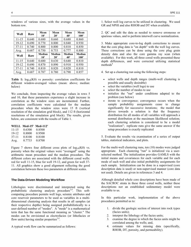
The relationship between plug permeability (K0) and plug porosity for the three cored wells is shown in Figure 6. Despite linear-like "cloud" trends there is not a strong linear relationship between the logarithm of permeability (K0) and porosity for any of the wells. This is not unexpected because the reservoir is made of different depositional facies each of which might be expected to have different porosity-permeability relationships. Mathematical analyses were performed to investigate the levels of correlation between log10(K0) and porosity. We calculated two different central measures for porosity and logarithm of permeability (K0) for all samples. These central measures were an arithmetic mean value and a median value corresponding to an adopted size-window around the sample depth. For instance, if a 10-point arithmetic mean is used, a moving window consisting of 5 points above and 5 points below a sampled depth is used to compute the arithmetic mean value of the 10 points at the center of the window. Likewise, if a 10-point median filter is selected, a moving window is made for 10 contiguous points, and the mid-point is replaced by the median of all 10 points. Table 1 shows correlation coefficients for these experiments for the three cored wells. Well names are in the first column and correlations using raw data are in the second column. The middle three rows of the upper five rows are results using mean values within windows of various sizes, with the average values in the fifth row. The middle three rows of the lower five rows are results using median values tithing

SPE 111 4

windows of various sizes, with the average values in the bottom row.

Well Raw Mean 10'

Mean 20'

Mean 40'

Mean 100'

11-15 0.640 0.680 0.660 0.680 0.860 19-12 0.690 0.770 0.800 0.840 0.930 37-11 0.740 0.800 0.800 0.810 0.850 Avg. 0.687 0.750 0.753 0.777 0.880

Well Raw Median 10'

Median 20'

Median 40'

Median 100'

11-15 0.640 0.680 0.630 0.640 0.810 19-12 0.690 0.870 0.890 0.910 0.950 37-11 0.740 0.810 0.820 0.820 0.810 Avg. 0.687 0.787 0.780 0.790 0.857

Table 1: log10(K0) vs porosity: correlation coefficients for different window-averaged values (mean: above; median: below)

We conclude, from inspecting the average values in rows 5 and 10, that these parameters experience a slight increase in correlation as the window sizes are incremented. Further, correlation coefficients were calculated for the median procedure when the window sizes were 15 ft (vertical resolution of the simulation grid block), and 112 ft (horizontal resolutions of the simulation grid block). The results, given below, are consistent with the results of Table 1. WELL Med-15' Med-112' 11-15 0.6300 0.8500 19-12 0.8800 0.9500 37-11 0.8100 0.8100 Avg. 0.7733 0.8700 Figure 7 shows four different cross plots of log10(K0) vs. porosity when the original values were “averaged” using the arithmetic mean procedure and the median procedure. The different colors are associated with the different cored wells: red for well 11-15, blue for well 19-12, and green for well 37-11. All graphics show a good alignment reflecting the good correlation between these two parameters at different scales.

The Data-Driven Modeling Workflow

Lithologies were discriminated and interpreted using the probabilistic clustering analysis procedure3,4. This soft-computing procedure permits well logs, seismic attributes and core reservoir parameters to be used as variables in a multi-dimensional clustering analysis that results in all samples (at their respective depths) being assigned probabilistically to a user-defined number of "modes". A "mode" is a mathematical term that has the same functional meaning as "cluster." The modes can be envisioned as electrofacies (or lithofacies or flow units) having similar properties3,4. A typical work flow can be summarized as follows:

1. Select well log curves to be utilized in clustering. We used GR and NPHI and also RHOB and DT when available. 2. QC and edit the data as needed to remove erroneous or spurious values, and to perform interwell curve normalization. 3. Make appropriate core-to-log depth corrections to ensure that the core plug data is "on depth" with the well log curves. These corrections can be done using the core plug grain density data and also the core gamma ray scan (when available). For this work, all three cored wells presented these depth differences, and were corrected utilizing statistical methods8 4. Set up a clustering run using the following steps: • select wells and depth ranges (multi-well clustering is

possible and usually desirable) • select the variables (well logs) to use • select the number of modes to use • initialize the "run" under conditions adapted to the

problem (see below) • iterate to convergence; convergence occurs when the

sample probability assignments cease to change significantly for successive iterations; the model that drives towards a solution is that the frequency distribution for all modes of all variables will approach a normal distribution at the maximum likelihood solution; each clustering solution is considered to be a model "realization"; replicate runs give the same answer if the setup procedure is exactly replicated

5. Evaluate the results via examination of a series of output tables, statistical indicators, and plots. For the multi-well clustering runs, ten (10) modes were judged appropriate. Each clustering "run" is initialized via a user-selected method. The initialization provides GAMLS with the initial means and covariances for each variable and for each mode of each well and also initial probability assignments for each sample. Initialization can be done in a supervised (core description data is used) or non-supervised manner (core data not used). Details are given in references 3 and 4. Although detailed whole core descriptions have been made of the SACROC strata in these three cored wells, neither these descriptions nor an established sedimentary model were available to us. In this particular work, implementation of the above procedures permitted us to:

1. divide the geologic section of interest into rock types (facies units);

2. interpret the lithology of the facies units; 3. examine the degree to which the facies units might be

correlated among the wells; and, 4. estimate values for missing data (specifically,

RHOB, DT, porosity, and permeability).

SPE 111 5

Discrimination and Interpretation of Facies Units If the modes are considered to be facies units, then the clustering process automatically discriminates the clustered depth intervals into facies units. Since the sample assignments are probabilistic, each sample can be assigned probabilistically to more than one facies unit. This is referred to as the “fuzzy” probability assignment, and is in accord with the idea that although ideal end-member rock types might exist (e.g., "clean" sandstone, "pure" limestone …), many rocks might have a composition intermediate between two or more end-member rock types. In a depth plot, the “fuzzy” probabilistic assignments are displayed as a stacked bar chart on a horizontal axis with axis ranging from zero (probability) at left to 1.0 (probability) at right. The sum of the mode probability assignments at each depth or sample is 1.0 (see, for instance, Figures 13, 15, 17). The "fuzzy" probability assignments can also be displayed as "crisp" assignments at each depth. The crisp mode assignment is the mode (facies unit) which has the highest fuzzy assignment, so at each depth a unique and definitive mode is declared. Contiguous crisp assignments in depth to the same mode define a "bed". Lithology assignments for each of the clustering modes (facies units) can then be assigned. This is based largely on GR signal for clastic rocks and apparent grain density for carbonate rocks10. Depth plots that display the probability assignments of all samples can be used to provide an easy method for visual examination and interpretation.

A major feature of this soft-computing approach is that values for missing (null) data can be generated during the clustering process. Data can be estimated for any curve that is used as a clustering variable. This means that missing log data can be generated during a clustering run. As discussed above, this procedure was used to generate RHOB and DT curves for wells that did not have these logs. Alternatively, AI_log curves were generated in wells with no RHOB and DT using clustering runs that included AI computed from RHOB and DT in wells that had RHOB and DT. Also, since only three wells had core plug data, this "estimation" capability was also used to generate core-scale porosity and permeability values for non-cored wells. This procedure is discussed more fully below. The term "facies" is used above as the name for a group of samples that have similar well log character as defined by a cluster analysis. The term "electrofacies" would be appropriate if all of the variables used in the clustering run were curves obtained from well log "tools". If the assumption is made that the well log curves are responding to lithology differences, then the term "lithofacies" would also be appropriate for the clustered groups. If one or more of the variables is a flow property (such as permeability) or is related to a flow property (which most well log curves are), then the term "flow unit" would also be appropriate. Here, we use the term “mode”, "facies", “rock type”, and "flow unit" interchangeably.

Reservoir Quality of Facies and Flow Units A major goal of this study is to define flow units and to determine their Reservoir Quality (RQ). We here use RQ to mean the porosity, permeability, bed thickness, and lateral bed continuity of the flow units. But, only porosity and permeability are evaluated in a quantitative manner. If facies units are considered to be equivalent to flow units (see discussion above), then flow units can be defined by clustering analyses using well log curves as variables or a combination of well log curves and core permeability and core porosity. Multiple clustering runs can be made where each run uses a different suite of variables. Each clustering run provides a different flow unit realization. Ideally, comparison of different clustering realizations would result in similar flow unit realizations. There are several different work flows that can result in determination of the RQ of flow unit realizations. It is not obvious, a priori, which work flow will produce the most realistic (closest to the "truth") flow unit realization and which work flow will produce the most credible definition of RQ for any given flow unit realization. However, it will be shown below that the modeling procedure is quite robust in that the porosity and permeability profiles obtained are largely independent of the particular work flow used. Since only three reliable cored wells were available, and only one of them is near to the center of the study area, the database for building a model for estimating porosity and permeability for the non-cored wells was limited in terms of areal extent across the studied area. However, because the cored wells were plugged every foot over a depth range of about 600 to 900 feet each, a considerable amount of core data was available for use For each clustering run, or series of clustering runs, the realization provides the following information for each flow unit: • the arithmetic mean and standard deviation of porosity, • the arithmetic mean and standard deviation of the

logarithm (base 10) of permeability, • the total bed thickness, the number of beds, and the

average bed thickness for the original beds (defined by clustering),

• qualitative assessment of well-to-well lateral continuity of each flow unit. This is done by generating for each well either a depth plot of the “fuzzy” probabilistic assignment or a depth plot of the “crisp” (mode) assignment and correlating these among wells by visual examination.

SPE 111 6

Estimation of Porosity and Permeability in Non-Cored Wells The basic approach is to perform a clustering run using one or more cored wells with core porosity and/or core permeability as variables along with a selected log curve suite as variables. For any non-cored wells included in the clustering run, estimates of core porosity and/or core permeability can be automatically made during the clustering process. Choices to be made for any given clustering run are: • how many cored wells to include, • whether only one or both core porosity and core

permeability should be included for the cored wells, • which non-cored wells must be included, and • which log curve variables should be included.

Another choice is whether one should define flow units using a clustering run that does not use core data as variables, or to define flow units using a clustering run that does use core data as variables. The former approach would require the determination of porosity and permeability profiles using a clustering run(s) that includes core porosity and/or permeability and then assignment of these profiles to a determined facies using a clustering run that utilized only log curves as variables. The alternative would be to determine both the facies and the profiles for porosity and permeability in the same clustering run. For logistical and work flow purposes, wells were divided into three groups: • Group G1 (3 wells total, with 1 in the central study area)

are those wells with GR, NPHI, RHOB, DT logs and with core data. The common core measurements for the cored wells were porosity, two horizontal permeabilities (K0 and K90), vertical permeability (Kv), percentage of fluorescence, and grain density data. Although only well 37-11 was in the central study area, the other two cored wells (11-15 and 19-12) were also used.

• Group G2 (9 wells total, with 3 in the central study area)

are those wells with GR, NPHI, RHOB and DT logs, but without core data. The three wells in the central study area are 33-15, 38-6 and 59-5. The other six wells (34-12, 37-10, 56-16, 56-17, 56-18, and 58-4) are distributed around the central study area. The most distant of these is well 34-12 which is about 2,500 feet from the central study area.

• Group G3 (25 wells total, with 18 in the central study

area) are those wells with only GR and NPHI logs. The seven wells not within the central study area are within 1400 feet of the study area.

Since most of the wells had no RHOB or DT logs, the decision as to whether to "fill in" the “ideal” log suite by estimating both RHOB and DT profiles for these wells (using the clustering methods), or to combine these two variables into

only one variable, acoustic impedance (AI_log), also needed to be made. Both approaches were tested. The latter method (calculation of log AI_log) provided the opportunity of having a log-based parameter that could possibly be correlated with the seismic acoustic impedance and that could also be used in clustering runs that included both well log and seismic attributes. Also, the use of AI_log instead of RHOB and DT decreases by one the number of variables when clustering processes are later carried out using G3 wells (wells having only GR and NPHI). To test the effectiveness of using AI_log instead of RHOB and DT in order to predict porosity and permeability values, clustering runs were done both ways. Predicted porosity and permeability values generated using the clustering run that utilized GR, NPHI and AI_log, (cluster run C9) were not significantly different from the predicted values generated using the clustering run that utilized GR, NPHI, RHOB and DT (cluster run C1AA). Both clustering runs also included as variables the core porosity and core permeability (log10) from wells 37-11 and 19-12 (cored well 11-15 was preserved as a "hold out" well and so was not included in the clustering runs.). The results are shown in Figures 8-10. Figure 8 shows two crossplots comparing predicted values of porosity (left plot) and logarithm of permeability (right plot) using cluster run C1AA, versus the corresponding values obtained using cluster run C9. Results for cored wells 19-12 (green), and 11-15 (red); and for the non-cored well 33-15 (blue) were superimposed in both plots. The table below shows the strong linear correlations in all three wells for the predictions of both porosity and log10 permeability computed using the two methods.

Well Porosity (r) Permeability (r) 11-15 0.96 0.97 19-12 0.93 0.97 33-15 0.97 0.99

Figure 9 shows depth plots for predicted porosity and permeability for wells 33-15, 11-15, and 19-12. Predicted porosity using C1AA (dark blue) and C9 (light blue) are plotted in the same tracks. The scale is 0.0 (left) to 0.30 (right) Likewise, predicted log10 permeability using C1AA (dark green) and C9 (light green) are plotted in the same tracks. The scale is -3 (left) to +3.0 (right). It is clear that there is generally excellent agreement in the predicted values of both porosity and log10 permeability using both methods. Finally, in Figure 10, predicted porosity (two blue symbols) and the logarithm of permeability (two green symbols) are plotted with actual core porosity and permeability data (red symbols) for cored wells 11-15 and 19-12. The results indicate that predicted values of porosity and log10 permeability are close to the actual values using both prediction methods. Note that these results are the results of an "internal holdout" test in which the core values of the two cored wells were used in the clustering runs of the 12 wells used to establish the models.

SPE 111 7

During the "predictions" clustering runs, the core values were held out. So, these results indicate the accuracy of predicting core values in wells which were actually included in the development of the prediction model. The procedure for combining RHOB and DT into AI_log and then using AI_log as a clustering variable is herein termed the "P&P via AI" method. This method involves several clustering runs which included AI_log, selected additional log curves (NPHI and GR), plus one or both permeability and porosity. The end results are "predicted" profiles for porosity and permeability in non-cored wells. This "P&P via AI" method was done in the following step-wise manner: • Using wells of groups G1 and G2, a clustering procedure

was carried out which included only GR, NPHI, and AI_log as log parameters. Notice that all wells belonging to these two groups have actual data of the mentioned variables. The target of such procedure was to provide an “intelligence” device capable of predicting AI_log in wells without RHOB and DT (group G3). This first step also shows the feasibility of applying data-driven methods to simulate missing logs based on the presence of other.

• Considering that actual AI_log does not exist in wells of

group G3 (RHOB and DT are absent), it was necessary to provide these wells with AI_log values in order to complete the necessary set of logs for predicting core parameters values at them. The clustering software permits the use of a previous clustering run to predict missing values of one of the variables utilized in such run at other locations. In consequence, the clustering results of the previous step were utilized to predict AI_log at wells in group G3. This action allowed wells from group G3 to complete the set of parameters necessary for later prediction of porosity and permeability values at core-scale based on the presence of GR, NPHI and AI_log.

• The next step was to generate core porosity and core

permeability curves at wells belonging to groups G2 and G3. This task was executed individually for each group and under different conditions. Firstly, core porosity and core permeability values were simultaneously generated at wells in group G2. Utilizing wells in groups G1 and G2, a clustering analysis was run with actual data GR, NPHI, and AI_log of both groups, and core P&P measures at wells belonging only to group G1. This clustering analysis resulted in the generation of simulated core parameters values on wells of group G2. This first step avoids the use of predicted AI_log curves of G3 wells as an input, and takes full advantage of the actual data of G1 and G2 wells. The second step in the generation of core parameters curves was to generate porosity and permeability values at wells belonging to the group G3. Using all well groups, a clustering procedure was executed with the following characteristics: from G1 wells, actual GR, NPHI, AI_log, and core P&P parameters were included; from G2 wells,

the input was constituted by actual GR, NPHI, and AI_log jointly with the pseudo core P&P parameters curves generated previously; from G3 wells, actual GR and NPHI, and predicted AI_log were utilized. This clustering step resulted in the generation of pseudo core parameters estimated values at wells belonging to group G3.

Below, Tables 2 and 3 summarize some of the clustering runs followed in the “P&P via AI” method. Table 2 gives the parameters (clustering variables) and wells used. Table 3 indicates the clustering goal. Additional clustering runs, not discussed here, were made in the search for an optimum work flow.

Cluster Variables Wells

C2 GR, NPHI, AI G1 + G2 C9 GR, NPHI, AI, POR, K0 G1 + G2 C9_K90 GR, NPHI, AI, POR, K90 G1 + G2 C9_Kv GR, NPHI, AI, POR, Kv G1 + G2 C10 GR, NPHI, AI, POR G1 + G2 + G3 C12 GR, NPHI, AI, POR, K0 G1 + G2 + G3 C12_K90 GR, NPHI, AI, POR, K90 G1 + G2 + G3 C12_Kv GR, NPHI, AI, POR, Kv G1 + G2 + G3

Table 2: Summary of the clustering procedures that constitutes the “P&P Via AI” Method for predicting core-scale P&P estimates. Variables and utilized wells.

Cluster Objective

C2 Used for predicting AI on G3 wells (well 11-15 included)

C9 Used for estimating POR and K0 on wells only of G2 (well 11-15 included)

C9_K90 Used for estimating K90 only on G2 wells (C9-POR used on G2 wells)

C9_Kv Used for estimating Kv only on G2 wells (C9-POR used on G2 wells)

C10 Used for estimating POR only on G3 wells (using C9-POR estimates on G2 wells)

C12 Used for estimating K0 on only G3 wells (using C9-POR and C9-K0 estimates on G2 wells, and C10-POR estimates on G3 wells)

C12_K90 Used for estimating K90 on only G3 wells (using C9-POR and C9-K90 estimates on G2 wells, and C10-POR estimates on G3 wells)

C12_Kv Used for estimating Kv on only G3 wells (using C9-POR and C9-Kv estimates on G2 wells, and C10-POR estimates on G3 wells)

Table 3: Summary of the clustering procedures that constitutes the “P&P Via AI” Method for predicting core-scale P&P estimates. Cluster objective.

Three of these clusters (C1, C7, and C8) did not include cored well 11-15; that well was used as a "hold out" well utilized for testing the accuracy of the predictions. The other clusters were used in various tests to help optimize the work flow.

SPE 111 8

Figure 11 shows tracks of AI_log, core porosity, and core log10(K0) respectively for cored well 11-15, the hold-out well. Actual values are in red and predicted values are in blue. These results were obtained during the sequence of different clustering runs done during establishing the “P&P via AI” method. For instance, cluster C1 was the first clustering run used to predict AI_log at wells. This cluster C1 had identical conditions to cluster C2 except that well 11-15 was excluded. The first two tracks indicate that agreement between predicted values and actual values are pretty good. In the track for log10(KO), we can appreciate that spatial tendencies are reproduced; however, larger numerical differences between actual and predicted values are evident. Figure 12 shows cross plots of predicted vs. actual values. AI_log is shown at left; porosity is seen at center, and log10(KO) is exposed at left. All cross plots show a good alignment reflecting a definitive correlation between predicted and actual values. The corresponding correlation coefficients (r) are 0.94 for AI_log, 0.74 for porosity, and 0.59 for log10(KO). As it can be expected for permeability, its prediction is the least accurate in absolute terms. However, the vertical variability of permeability is reproduced quite well; the predictions simply do not fully capture the extreme values. Nevertheless, reproducing the vertical variability is arguably the most important objective when utilizing such results for reservoir flow simulation purposes. This subject is revisited in Appendix A, particularly with the discussion related to Figure A-8.

Cluster run C8 was a precursor to cluster run C9 in providing estimates values of porosity and permeability. Cluster run C8 set up was identical to cluster C9 except that well 11-15 was not included. Again (second track) porosity values were excellently reproduced. However, permeability (log10) predicted values were not as good as the porosity predicted values. This is discussed in more detail below.

In summary, the “P&P via AI” method allowed populating all wells included in the selected subregion with core-scale P&P curves which facilitated the application of geostatistical methods for reservoir characterization of the subregion. Modes, Beds, and Flow Units: Discussion Five clustering runs were made to determine how the results would vary with run setup conditions. This is important since the modes (flow units) are determined largely from the results of the clustering runs. The setup for these clustering runs is summarized in Table 4.

The porosity and permeability (P&P) used was that from the “P&P via AI” method (described above). This data is inserted into the digital log files so that even if the P&P data are not used as variables in a given clustering run, the mean and standard deviation of that data are automatically included in output tables for examination

Cluster Variables & N° of Modes Wells

C1A GR, NPHI, RHOB, DT; 10 modes G1 + G2

C1B

as C1A but 19 additional wells with no

RHOB or DT; 10 modes

G1 + G2 + G3

C1C as C1A but also P&P from 37-11; 10 modes G1 + G2

C1D as C1A but also P&P from 37-11; 25 modes G1 + G2

C1E as C1A but also P&P

from 37-11 & 11-15; 10 modes

G1 + G2

Table 4: Summary of Clustering Procedures Utilized to

Analyze the Robustness of Flow Unit Definition.

The setup and results from cluster run C1A is described in some detail here. Each of the other clustering runs generated output in the same format as that for C1A. Cluster C1A used log data from three cored wells and nine uncored wells (groups G1 and G2). The cored wells were 37-11 (in the center of the study area) and two wells, 19-12 and 11-15, located to the NNW and NW about 8,000 ft from the center of the study area. The used uncored wells were 33-15, 23-12, 36-8, 37-10, 56-16, 56-17, 56-18, 58-4, and 59-5. Except for well 34-12, these uncored wells were within about 5,000 ft of well 37-11.

The upper-most depth used for each well in these cluster runs was slightly above or at the top of the “Canyon Reef” as picked by the dataset provided by Kinder Morgan. Because there was no attempt to restrict the depth ranges clustered to the Cisco and Canyon sections, the tops and bottoms of the intervals selected for clustering extended up into the Wolfcamp Shale for most wells and also likely extended down into non-productive water zone of the Canyon or below the Canyon Formation into the underlying Strawn Formation. Clustering variables were RHOB, NPHI, GR, and DT. All of the wells had continuous logs for these curves, so there was no missing data. An initialization method ("large covariance") was used that puts no emphasis on any of the particular variables. Ten modes were selected for clustering. Clustering results and raw logs are shown for two of the cored wells in Figure 13. For each well, the first track shows GR and DT and the second track show RHOB and NPHI. The third and fourth tracks are core porosity and core permeability, respectively. The fifth track is a Cumulative Mode Probability (CMP) plot which displays the “fuzzy” probabilistic assignment at each depth (the horizontal axis is fractional probability). The sixth track is a "beds" plot which displays the “crisp” (mode) assignment at each depth (only the mode is shown that has the highest probability for each sample depth).

SPE 111 9

The CMP plot is also termed a "fuzzy" plot and the "beds" plot is also termed a "crisp" plot. We used a combination of the “ModeAssign” routine (which gives default lithologies for each mode), some user decisions, and previously reported information about the SACROC to interpret all of the modes that comprise the Cisco and Canyon interval to be limestones. Independent of the core data, Mode 10 (M10) was interpreted to have the best RQ because it had the highest mean NPHI value (0.13) which in turn suggested that it had the highest porosity in these fairly "pure" calcite-rich rocks. That is, in these clay-poor rocks, NPHI appears to be a fair indicator of porosity. The relative ranking of RQ based on mean NPHI values was confirmed by the core data. A table generated as part of the clustering results that gives mean core porosity and permeability for each mode showed that M10 generally had the best RQ in the cored wells. This mode, the apparent "best" limestone, was named (M10_LsBest). For plotting purposes, this mode was assigned a bright red color. M10 plus six other modes, also interpreted to be limestones, comprise nearly all the Cisco and Canyon interval. Of the other six limestone modes, three had relatively high apparent porosities based on the mean NPHI values: M3_LS1 with mean NPHI = 0.12, and M5_LS2 and M8_LS3 with mean NPHI = 0.11. The other three limestone modes had relatively low apparent porosities: M1, M7, and M2 with mean NPHI values of 0.04, 0.04, and 0.01, respectively. To discriminate among the "high porosity" modes and the "low porosity" modes, M3, M5, and M8 were colored deep pink, hot pink, and pink, respectively, and the other limestone modes were shades of blue (the deeper the blue shade, the lower the porosity). The modes assigned as siltstones (M9_Slt, green) and shales (M6_Sh1, M4_Sh2, grays) were mostly (but not entirely) above the carbonate sections and presumably mostly in the overlying Wolfcamp shales. The upsection change from carbonates to shales indicated by the clustering results is generally sharp and provides a good way to pick the contact between the Cisco and the Wolfcamp. Figure 14 is a representative cross plot that shows samples color coded to the crisp assignment. The ellipses are 4D ellipsoids projected onto the RHOB-NPHI plane, and are drawn at approximately two standard deviations from the centre (mean values) of each ellipsoid. Figure 15 shows C1A clustering results (first two tracks) and raw well logs (far right track) for non-cored well 33-15. The permeability and porosity values plotted in tracks 3 and 4, respectively, are predicted values using the "P&P via AI" method (cluster run C9). So, this is an example of deriving flow units from one clustering run (C1A), deriving predicted porosity and permeability from another (series) of clustering runs (C9), and then relating the flow units to these two RQ parameters. This was done for all of the non-cored wells in C1A.

It is obvious that the highest porosities and permeabilities are in the zones indicated by the bright red Mode 10 color. It is also clear that the four modes with highest RQ (red and pink colors) have transitional contacts with one another but have fairly sharp contacts with the modes with lower RQ (blue colors). That is, the reds and pinks could be considered as one series of closely related flow units and the blues as a second series of closely related flow units. With any clustering analysis, two tables (fuzzy statistics and crisp statistics) give, for each well in the clustering run, the mean and standard deviation of all curves in the well log "curves" file for each mode, the percentage of samples assigned to each mode, the total footage assigned to each mode, the number of beds defined by each mode, the mean bed thickness for each mode, and the mean probability assignment of the crisp mode for each mode. This information is useful for evaluating the overall RQ of each mode. Figure 16 shows a cross plot of predicted permeability (log10) versus predicted porosity for non-cored well 33-15. Again, the predicted permeability and porosity values are from the "P&P_AI" method (cluster C9). The samples are color coded by mode from C1A. Correlations by mode are given in the legend. The shale and siltstone samples (grays and green) are almost all from the overlying shale. The main point here is that RQ in terms of porosity and permeability varies by mode and the modeled (predicted) porosity and permeability have fairly good correlations. Figure 17 shows CMP plots for Well 37-11 for the five clustering runs tabulated in Table 4. In each CMP plot, the generally three to four red-colored modes represent the best reservoir quality limestones, with porosities ranging from 10 to 14 percent, and the generally three to four blue-colored modes represent poor reservoir quality limestones with porosities generally less than 6 percent. The permeabilities have a similar division into a high range and a low range. Most of the red-colored modes have permeabilities greater than 2.5 md and most of the blue-colored modes have permeabilities less than 2.5 md. In the simplest reservoir quality classification, the limestone modes could be divided into only two: good (red) and poor (blue). Regardless of the realization, the good RQ limestones are clearly discriminated from the poor RQ limestone This indicates a fundamental difference in depositional or diagenetic features that has affected reservoir quality in the red- versus blue-colored modes. The poor RQ limestones represent barriers to vertical flow. If the good (or poor) RQ units pinch out laterally, then this presents a significant problem to be addressed via geostatistical modeling in the development of geological and reservoir flow models. Analysis of Some Oriented Cross Sections In order to have a better understanding of the lateral and vertical variability of the flow units in the studied region, two E-W cross sections and one N-S cross section were generated

SPE 111 10

through the study area. Figure 18 presents a plan view of these cross sections named A-A’, B-B’, and C-C’.

Figure 19 shows N-S cross section C-C’. Bright red represents best reservoir quality (RQ) and deepest blue is poorest RQ. Here, the section has been divided into three zones conceived as flow unit "groups" and coded as A, B, and C respectively from top to bottom. Based on results of cluster C1A, zone B has the best overall RQ and it is separated from the overlying zone A and the underlying zone C by apparently laterally continuous flow-barrier units of low RQ (dark blue units). It is also clear that some individual flow units exist within zones A, B and C that can be correlated among some of the wells Figure 20 represents cross section A-A’. The facies (flow units) are again taken from cluster run C1A. The thickest and best RQ units are in the upper half of the section The approximate positions of the zones A, B, and C shown in Figure 19 have been delineated at the location of well 37-5, Other cross sections were analyzed but were not shown here. For instance, in the cross section B-B’, approximate positions of the zones A, B, and C were easily found at well 59-1 but, in general, the zones and the individual flow units within the zones are less well-defined in this southern part of the study area. Regardless of how the wells were arranged in cross sections, it was clear that the upper half of the carbonate section is generally better reservoir quality than the lower half, and within the upper half there is a zone of "best" reservoir quality approximately between 6,400 and 6,600 feet. Also, the better interwell correlations between wells in the N-S cross section than in the E-W cross sections likely can be attributed to the overall depositional geometry of the reef deposits: N-S is more of a structural and depositional strike direction and E-W is more of a structural and depositional dip direction. The likely effects of the vertical and lateral distribution of the “good” RQ and “poor” RQ flow units on exploitation strategies are important. Low RQ zones that are laterally continuous would act as vertical flow barriers and tend to compartmentalize flow units causing any injected fluids to be “channeled” between the flow barriers. In consequence, local azimuthal anisotropy should be considered when planning injection well locations, perforation intervals, and sweep directions.

To help put these flow unit trends into a larger context, we summarize key points from Waite11 (1993). These summary comments refer to the Horseshoe Reef in general and all features mentioned might not occur locally in the Kelly-Snyder Field. Waite10 identified four 3rd order sequences in the reef. The sequence boundaries are marked by prominent seismic reflectors. Each of these boundaries apparently marks the end of an overall shallowing (drop in sealevel) and the onset of a major flooding episode (rise in sealevel). Shallowing episodes might have been sufficient to generate an interval of subaereal

erosion during maximum sea level drop during which time karsting and leaching (accompanied by enhanced porosity development?) occurred. Chronology of the sequences is via fusulinid foraminiferal biostratigraphy which divides the Pennsylvanian section into 14 zones (7 in the earlier Pennsylvanian Strawn and 7 in the later Pennsylvanian Canyon and Cisco (see Waite11, Figure 4). Each of the foraminiferal zones is interpreted to represent about 1 million years of deposition. The four 3rd-order sequences that have been recognized via seismic are marked by sequence boundaries (from oldest to youngest) at the top of the Strawn (top of foraminiferal zone DS7), at the top of the Canyon A (top of zone MC1), at the top of the Canyon B (top of zone MC4), and at the top of the Canyon B/Cisco (top of zone MC7). Onlapping relatively deep water Permian Wolfcampian shales overlie the uppermost carbonate reef deposits of foraminiferal zone MC4. From well log analysis, 4th and 5th order sequences have been interpreted within some of the 3rd order sequences and the tops of some of these higher-order sequences are interpreted to be exposure surfaces (see Waite11, Figure 9). Although the Canyon A (50-100 feet) is interpreted to be a single parasequence set, in at least one area of the Horseshoe Atoll, the Canyon B (0-400 feet) consists of at least seven parasequence sets. Each 3rd order sequence represents an evolution through time of carbonate deposits changing from platform to bank to reef mound. During each sequence, water became shallower and there was a decrease in the areal extent of the deposits often culminating in a "pinnacle" structure. Facies geometry of the four 3rd order sequences as interpreted from seismic indicate that the Strawn is a "mounded discontinuous" facies, the Canyon A is a "distinct clinoform" facies, the Canyon B is a "mounded coherent" facies, and the Canyon C/Cisco is a "lensoid" and/or "chaotic" facies. The rock types are mostly wackestones and packstones with occasional grainstones. With the above study by Waite11 for a model, we have attempted to correlate the data-driven defined flow units with his 3rd order sequences (Waite11, Figure 19). In general, our database did not permit us to identify the top of the Strawn using well logs (many of our logs stopped before penetrating the Strawn). Since that footage was not included in the clustering runs, we could not search for a sequence boundary there. In Figure 21, the 12 wells (G1 and G2 wells) used in C1A are positioned left-to-right according to relative structural position using a prominent low RQ “bed” near the bottom of the studied interval. There are two prominent horizons with relatively low average porosities and these were shown in Figure 19 as flow barriers with low RQ. These we suggest are the "top C1" (separating the Canyon A from the Canyon B) and the "top C4"

SPE 111 11

(separating the Canyon B from the Canyon C/Cisco) sequence boundaries of Waite11. These are shown in Figure 21 by the upper and lower yellow lines, and the lowermost of these happens to be the datum used for positioning the wells in Figure 21. Within the Canyon B, there are several cycles of low porosity units overlain by high porosity units. Within cored well 37-11, for instance, there are 12 to 14 of these cycles. We interpret these to be 4th order cycles. One of these cycles is more prominent than the others and we use it to subdivide the Canyon B into a lower Canyon B1 and an upper Canyon B2. This subdivision is shown as the middle yellow line in Figure 21. This provides a four-part division of strata between the Strawn and the Wolfcamp. Not surprisingly, the upper two of these divisions are coincident with the A and B and intervals depicted in Figures 19 and 20, and the next division down section would be coincident with the C interval if the C were not arbitrarily stopped at its bottom but extended down to the low porosity horizon interpreted to be the "top C1" sequence boundary. In summary, a two-step “soft-computing” procedure was developed that was capable of efficiently generating core-scale porosity and permeability profiles at well locations where no core data existed and where only GR and NPHI were available. In addition, rock types were identified and flow units were defined. Because the suitable logs for the creation of a direct Log-to-Core “intelligent” device were not present at all wells, it was necessary to create another intelligence tool, a Log-to-Log model, to provide values for missing information. This two-step “soft-computing” procedure provided core-scale estimates of P&P and rock types at well locations. So, with the goal of reservoir characterization of a relevant area in the SACROC Unit Platform as the field demonstration, this data-driven procedure was utilized to populate the studied subregion with pseudo core-scale profiles of porosity, permeability, and flow units. This provided the data needed for the direct application of geostatistical methods to build a 3D reservoir model.

The Geostatistical Approach The existence of twenty two (22) wells in the study area having foot-by-foot profiles of P&P was considered sufficient information to characterize directly the reservoir distributions of porosity and permeability. Stochastic simulation algorithms were utilized to provide reservoir models of porosity and permeability in the selected study region with different levels of vertical resolution. The goal is to generate reservoir parameter characterizations with an appropriate vertical resolution to aid the efficient characterization of this complex reservoir. The Geostatistical Context In general terms, hybrid simulation approaches that combine two or more conditional simulation techniques are used in a

geostatistical study12,13,14. A geostatistical reservoir characterization based on a hybrid approach usually consists firstly in building the reservoir architecture where the geometry of the units is established; then, determining the geological model where geobodies are populated with lithofacies, and finally generating the petrophysical model where distributions of typical reservoir parameters are assigned to each facies. Geostatistical simulation techniques are usually categorized using either pixel-based or object-based methods12,15. Pixel-based methods are largely used to characterize reservoir parameters like porosity and permeability, but they are not designed to explicitly reproduce geometric shapes as their final goal. Yet, they can be applied to model facies with unclear or undefined shapes. Object-based methods are suitable to describe reservoirs with certain geometric features, provided that adequate information (qualitative and/or quantitative) of the geometry of reservoir bodies is available12,15. They are frequently utilized for fluvial, deltaic, and deep marine depositional environments, and when a limited number of wells with conditioning data exist. In these types of environment, the shape of most facies, like channels, mouth bars, levees, and different types of shale, can be represented by discrete objects with well known geometric shapes. However, object-based modeling is less applicable to carbonate environments which have facies that exhibit serious post-depositional processes (dissolution, re-precipitation, dolomitization, fracturing, etc) that have deteriorated the geometry of their shape such that the utilization of known geometric objects and the estimation of their dimensions is problematic. Due to the above arguments, and given the existence of twenty two (22) wells in the study area with profiles of P&P, variogram analysis was directly applied to this data to determine possible patterns of spatial variability of these parameters. With the derived variogram models, the Sequential Gaussian Simulation (SGS) algorithm conditioned to the well data was used to generate multiple reservoir distributions of porosity and permeability at interwell locations. Corresponding central scenarios of P&P were generated from these characterizations and were utilized as input into the next step, reservoir simulation performance, where production data have to be honored. Stratigraphic Coordinates An important consideration in most 3D geostatistical applications is the design of an appropriate coordinate system. Due to its complex geological processes, the SACROC anisotropy directions vary throughout the area with the local dips. For the variogram analysis and for the simulations, the data location coordinates were transformed to stratigraphic coordinates12.. This coordinates transformation is commonly utilized for folded or variable thickness geologic bodies where various geometrical arguments can be used to manipulate the stratigraphy. However, for this small subregion of SACROC, based on the small variability of its thickness (coefficient of

SPE 111 12

variation is 0.075), we assumed a simple reservoir geometry with a flat stratigraphic top and bottom. This stratigraphic coordinate system relocates observations proportionally, based on their distance from the top and base of the body (new coordinates relative to marker horizons). The coordinates transform proposed here is given by:

y)]top(x,-[z*y)]top(x,-y)[bott(x,

T top z'

y y' x x'

min +=

== ..........(2)

where (x,y,z) are the original Cartesian coordinates, and (x’,y’,z’) are the transformed stratigraphic coordinates. The coordinate z is reset to vary proportionally in a numerical interval of constant length given by T. The value of T can be any meaningful thickness of the reservoir or analyzed area - for instance, the average thickness of all sampled wells in the region, the maximum thickness, etc. For this study, the selected length was 900 feet based on the 898 feet of core data sampled at location of well 37-11 inside the central study area. The value top(x,y) is the top depth of the original geological unit at location (x,y); the value bott(x,y) is the bottom depth of the of the studied geological body at location (x,y), and topmin is the minimum value of the group of top values sampled in this subregion (3,662 ft subsea for this SACROC subregion). The purpose of this transformation is “to straighten out" a geologic body considered as contorted or with variable thickness, and to represent it as an equivalent box-shaped body for purposes of spatial correlation analysis and modeling. Variogram Analysis Reservoir parameters are modeled as random variables that vary continuously in space. The basic geostatistical tool used to quantify the spatial variability of a reservoir parameter is the experimental semivariogram (herein "variogram"). The experimental variogram is used for identifying the underlying spatial pattern and identifying trends; it reveals the randomness and the structured aspects of the spatial dispersion. In essence, it is a plot which illustrates the way in which the dissimilarity between sample values is related to the separation distance and direction between the sample values. The definitive spatial pattern of reservoir parameters for characterization purposes using stochastic simulation algorithms is finally established when authorized mathematical functions are fitted on the experimental variogram obtained from the data (the mathematical condition requested for these functions is known as the "positive definite condition") 12,13,14. This variogram model provides the spatial correlation between parameter samples in terms of the distance and the direction between samples, and reflects the continuity and spatial variability of the studied reservoir parameter. The variogram model is the main input required by the simulation procedure SGS which produces equiprobable

characterizations of reservoir parameters constrained by the data. The more commonly used variogram models are the exponential, spherical, Gaussian, power models, hole effect models (cyclic), and the pure nugget effect. Equations for all these models can be found in references 12, 13, and 14. The spherical model can be considered as the variogram resulting from a large variety of natural processes, and is the most popular model utilized by practitioners in tasks of stochastic reservoir characterization. This work was not an exception. Spherical models were adjusted to all analyzed experimental variograms. For the variogram analysis of SACROC, actual values and pseudo values of core porosity, core permeability, and rock types were utilized to calculate corresponding experimental variograms. In order to calculate the experimental variograms of P&P and modes (rock types), a stratigraphic or conformal transformation of vertical coordinates was first carried out in order to compare samples from similar stratigraphic horizons and to avoid typical differences resulting from horizontal slicing based on the original coordinate system. This kind of “unrolling” of the structure allows comparison of sample values at the same “stratigraphic horizon” when the experimental variogram is calculated. Comparisons of samples under this premise are considered geologically consistent because it can be expected that reservoir parameter values at the same “stratigraphic horizon” have more depositional similarities. In consequence, resulting experimental variograms can better reveal the “hidden” spatial behavior of the variable under analysis. Due to the dimensions of the subregion under study, to the significant number of wells included in it having foot-by-foot profiles of porosity and permeability, and to practical considerations related with the posterior task of the flow simulation (data availability, simulation objectives, grid definition, software, etc.), it was decided to characterize directly the distribution of P&P without the consideration of the rock type parameter (mode) as a possible guide. In addition, the origin of the foot-by-foot P&P pseudo values at well locations is narrowly tied to the corresponding foot-by-foot mode or rock type values at the same well locations, so this fact also favors the direct and less elaborate approach. As a consequence of this decision, direct data of P&P was utilized for the variogram analysis, and in the application of the SGS algorithm. As mentioned above, an alternative approach is commonly used when facies or rock type descriptions are available at well locations. First, this is done to model a spatial distribution of facies using adequate geostatistical algorithms, and later to "fill” these spatial “entities” with porosity, permeability, and water saturation values following the corresponding spatial behavior (variogram model) of each parameter in each rock type. Although this approach was not utilized here, to keep things simple for the posterior reservoir simulation task, indicator variogram analyses of modes (rock types) and

SPE 111 13

variography studies of P&P for each rock type were carried out in order to complement the global variography of P&P. The use of Gaussian techniques requires a prior Gaussian transform of the data and the complete variogram analysis of these transformed data (experimental and modeling tasks). This transformation automatically sets the sill value of the variogram to be 1 (its theoretical value). The utilized software was the Stanford Geostatistical Earth Modeling Software (SGEMS)16, which is software for 3D geostatistical modeling that implements some classical geostatistics algorithms, as well as additional developments made at Stanford University. Its geostatistical routines includes Kriging, Cokriging, Sequential Gaussian Simulation, Sequential Indicator Simulation, and other geostatistical tools for basic statistics, variography, post simulation analysis, etc. This public domain software was used to compute the experimental variograms of normalized porosity values, normalized permeability measurements (log10), and rock-types in both the vertical and horizontal directions, and fit spherical variogram models to the experimental variograms, as long as there was adequate data to estimate the experimental variogram in the considered direction and for the considered variable. In summary, the parameters describing the spatial correlation (nugget effect, sill, number of structures, types of structures, and ranges) were obtained graphically by plotting the experimental variogram against intersample distances and then fitting corresponding theoretical models. The nugget effect value and general structure of the models were obtained from vertical variograms, and were extended to horizontal (areal) variograms. Directional variograms were constructed in eight directions under the assumption that the stratigraphic transformation of coordinates produces the effect of sample pairs belong to the same bedding plane or stratigraphic horizon. Directional variograms describe the relationship between data pairs oriented in a specified direction. They are used to determine whether the spatially distributed data is anisotropic.

Anisotropy ellipses are typically constructed by plotting the range vs. the direction vector for each data set. In theory, a 3D-variogram analysis should offer the closest vision of the directional anisotropy of a reservoir parameter. In practice, the 3D analysis is generally calculated in the transformed space XYZ’ where the dip effects can be considered “diminished” or removed by the stratigraphic coordinates transformation. In consequence, most 3D variogram analyses can be conceived as 2D analyses in conformal beds, which essentially means that directional preferences in the dip direction are assimilated in the transformation. In this work, 2D areal and 1D vertical analyses were combined. Porosity Variography Modeling the spatial relationship of a reservoir attribute is one of the most important tasks in constructing reservoir characterization using geostatistical methodology. Multiple scales of heterogeneity can generally be found to a degree in all depositional settings. In the reef-carbonate depositional

environment of SACROC, different scales of variability can be seen, for instance, in variograms of porosity, and these different scales of variability are modeled using nested variograms (linear combinations). Porosity values at well locations (actual measurements and pseudo data) were initially normally transformed prior to the variography study. The variogram analysis conducted to evaluate spatial continuity in the vertical direction (see Figure 22) indicated a behavior that can be described as a combination of spherical (or exponential) and dampened hole-effect (cyclic) variograms. A hole-effect variogram is associated with geologic cyclicity. Due to the fact that geological processes can repeat over geologic time leading to cyclic variability of facies and petrophysical properties, a cyclic behavior can appear in experimental variograms12,17 . The experimental variogram can alternate from positive correlations to negative correlations at a length scale directly linked to the geologic cycles. In SACROC, this cyclicity effect in the vertical direction can be associated with the carbonate buildups. Relative sea level “rise and fall” occurred repeatedly, providing a variety of depositional environments and facies that repeat with geological time (seen in depth). However, this dampened hole-effect structure only applies in the vertical direction as it can be seen in Figure 23 where directional experimental variograms (normalized porosity) considering horizontal variability in several directions are simultaneously shown. For this reason, and the fact that both types of empirical variograms, vertical and horizontal, reach the unity sill, the experimental variogram in the vertical direction was modeled as a combination of a nugget effect component and two nested structures conceived as spherical models of spatial variability (i.e., the hole effect variogram model was not considered). The vertical variogram model, shown in Figure 22, superimposed with the experimental one, illustrates the correlation structures of the data and indicates that depositional environments and facies are primarily correlated at a shorter separation distance of 20 feet and more globally correlated at a larger correlation scale of 230 feet. This first range of 20 feet is half of an apparent period of 40 feet (geological cycles are not perfectly constant) shown on the dampened cyclic variations of the experimental variogram trajectory as separation distances increase. This behavior can also be observed on experimental variograms of some rock types (modes), and particularly coincided with the range found for reformulated modes 2 and 3 when the vertical variography of modes (rock types) was developed for a more simplified classification of only four modes (instead of the original ten modes). The analytical expression of this model12,13,14 is given by:

( ) ( ) 230hSph *0.35 20

hSph *0.55 0.1 γ(h) ++= .............(3)

SPE 111 14

where 0.1 is the nugget effect value, and 0.55 and 0.35 are variance values that can be considered as relative sills. Figure 23 shows eight superimposed experimental variograms of normalized porosity in the directions 0°, 30°, 45°, 60°, 90°, 120°, 135°, and 150°, where angles are measured clockwise from the axis North-South (0°). These horizontal variograms exhibit high nugget values, but they are not used in the model variogram. The nugget effect value is derived from the vertical variography since the horizontal and vertical variograms must share the same nugget value.

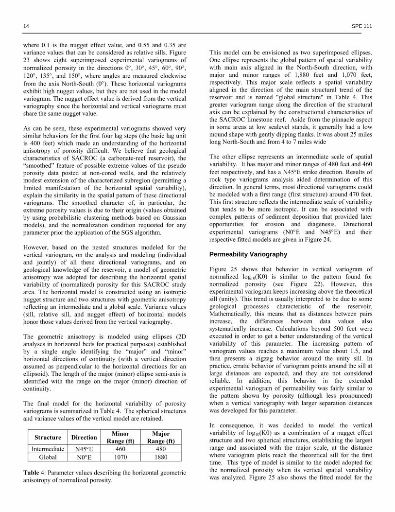
As can be seen, these experimental variograms showed very similar behaviors for the first four lag steps (the basic lag unit is 400 feet) which made an understanding of the horizontal anisotropy of porosity difficult. We believe that geological characteristics of SACROC (a carbonate-reef reservoir), the “smoothed” feature of possible extreme values of the pseudo porosity data posted at non-cored wells, and the relatively modest extension of the characterized subregion (permitting a limited manifestation of the horizontal spatial variability), explain the similarity in the spatial pattern of these directional variograms. The smoothed character of, in particular, the extreme porosity values is due to their origin (values obtained by using probabilistic clustering methods based on Gaussian models), and the normalization condition requested for any parameter prior the application of the SGS algorithm. However, based on the nested structures modeled for the vertical variogram, on the analysis and modeling (individual and jointly) of all these directional variograms, and on geological knowledge of the reservoir, a model of geometric anisotropy was adopted for describing the horizontal spatial variability of (normalized) porosity for this SACROC study area. The horizontal model is constructed using an isotropic nugget structure and two structures with geometric anisotropy reflecting an intermediate and a global scale. Variance values (sill, relative sill, and nugget effect) of horizontal models honor those values derived from the vertical variography. The geometric anisotropy is modeled using ellipses (2D analyses in horizontal beds for practical purposes) established by a single angle identifying the “major” and “minor” horizontal directions of continuity (with a vertical direction assumed as perpendicular to the horizontal directions for an ellipsoid). The length of the major (minor) ellipse semi-axis is identified with the range on the major (minor) direction of continuity. The final model for the horizontal variability of porosity variograms is summarized in Table 4. The spherical structures and variance values of the vertical model are retained.

Structure Direction Minor Range (ft)

Major Range (ft)

Intermediate N45°E 460 480 Global N0°E 1070 1880

Table 4: Parameter values describing the horizontal geometric anisotropy of normalized porosity.

This model can be envisioned as two superimposed ellipses. One ellipse represents the global pattern of spatial variability with main axis aligned in the North-South direction, with major and minor ranges of 1,880 feet and 1,070 feet, respectively. This major scale reflects a spatial variability aligned in the direction of the main structural trend of the reservoir and is named "global structure" in Table 4. This greater variogram range along the direction of the structural axis can be explained by the constructional characteristics of the SACROC limestone reef. Aside from the pinnacle aspect in some areas at low sealevel stands, it generally had a low mound shape with gently dipping flanks. It was about 25 miles long North-South and from 4 to 7 miles wide The other ellipse represents an intermediate scale of spatial variability. It has major and minor ranges of 480 feet and 460 feet respectively, and has a N45°E strike direction. Results of rock type variograms analysis aided determination of this direction. In general terms, most directional variograms could be modeled with a first range (first structure) around 470 feet. This first structure reflects the intermediate scale of variability that tends to be more isotropic. It can be associated with complex patterns of sediment deposition that provided later opportunities for erosion and diagenesis. Directional experimental variograms (N0°E and N45°E) and their respective fitted models are given in Figure 24. Permeability Variography Figure 25 shows that behavior in vertical variogram of normalized log10(K0) is similar to the pattern found for normalized porosity (see Figure 22). However, this experimental variogram keeps increasing above the theoretical sill (unity). This trend is usually interpreted to be due to some geological processes characteristic of the reservoir. Mathematically, this means that as distances between pairs increase, the differences between data values also systematically increase. Calculations beyond 500 feet were executed in order to get a better understanding of the vertical variability of this parameter. The increasing pattern of variogram values reaches a maximum value about 1.5, and then presents a zigzag behavior around the unity sill. In practice, erratic behavior of variogram points around the sill at large distances are expected, and they are not considered reliable. In addition, this behavior in the extended experimental variogram of permeability was fairly similar to the pattern shown by porosity (although less pronounced) when a vertical variography with larger separation distances was developed for this parameter. In consequence, it was decided to model the vertical variability of log10(K0) as a combination of a nugget effect structure and two spherical structures, establishing the largest range and associated with the major scale, at the distance where variogram plots reach the theoretical sill for the first time. This type of model is similar to the model adopted for the normalized porosity when its vertical spatial variability was analyzed. Figure 25 also shows the fitted model for the

SPE 111 15

vertical continuity of log10(K0). The corresponding analytical expression is given by:

( ) ( ) 400

hSph *0.42 20hSph *0.48 0.1 γ(h) ++= ..............(4)

Experimental variograms of normalized log10(K0) in the directions 0°, 30°, 45°, 60°, 90°, 120°, 135°, and 150° were calculated, but here omitted. All of them showed a behavior which appears to be changing in zigzag around the unity value (this might be considered as a pure nugget effect)12,13,14.A possible reason for this high variability in the log10(K0) variograms may be that permeability values are not coming from a single population. These experimental variograms complicate the development of a variogram model for the whole horizontal continuity of the normalized log10(K0). Due to the absence of satisfactory experimental evidence of the horizontal continuity of this parameter, and assuming, based on analyses of core data, that the logarithm of permeability and porosity are correlated, the building of the permeability variogram model describing its horizontal variability was “borrowed” from the variogram model of porosity but it preserved the original vertical variability derived from the vertical experimental variogram. This assumption was also supported by analyzing the cross variography between these two parameters (discussed below). When both vertical models (porosity and permeability) are compared, both models present a first range of 20 feet (intermediate scale) although they have different global scale ranges. The similarity between the first ranges permits the direct use of the same geometric anisotropy of porosity for the first structure of permeability. For the second global scale, the ratio between corresponding major scale ranges (permeability-range/porosity-range) was calculated to utilize this proportionality in determining ranges for the horizontal variability of permeability data relative to the equivalent porosity data18. This factor is approximately 1.74, and resultant variogram models for permeability were assumed similar to the porosity variogram models but with a global scale range augmented by a factor of 1.74. The same anisotropy ellipses of directionality were assumed. For the horizontal variogram models of normalized permeability, variance values are equal to those derived from the vertical variography. The final model for the horizontal variability of permeability variograms is summarized on Table 5.

Structure Direction Minor Range (ft)

Major Range (ft)

Intermediate N45°E 460 480 Global N0°E 1860 3270

Table 5: Parameter values describing the horizontal geometric anisotropy of normalized permeability.

Cross-Variogram Analysis Application of Gaussian algorithms to simulate a primary variable guided by a secondary correlated variable could require a model of the crossed spatial variability between both parameters12,13,14. As mentioned before, the logarithm of permeability is correlated to porosity, and this fact is also used to characterize the distribution of permeability in this subregion of SACROC. In consequence, a cross variography study was developed between normalized porosity and normalized logarithm of permeability in order to determine possible patterns of crossed continuity between these parameters. Figure 26 shows, at left, the vertical cross variability between normalized porosity and normalized permeability (log10). The experimental variogram presents very similar variability to the patterns previously found for normalized log10(K0) and for normalized porosity. Again, this experimental variogram increased above the theoretical sill (unity) ratifying the similar trend found in the vertical variography of these parameters when analyzed individually. Following previous variogram models as guidelines, the crossed vertical variability between porosity and log10(K0) was modeled as a combination of a nugget effect structure and two spherical structures. Superimposed to the vertical variogram is the corresponding fitted model of continuity. The analytical expression is given by:

( ) ( ) 375hSph *0.425 20

hSph *0.475 0.1 γ(h) ++= ..........(5)

In Figure 26, at right, eight experimental cross variograms of normalized log10(K0) and normalized porosity are shown in directions 0°, 30°, 45°, 60°, 90°, 120°, 135°, and 150°. These experimental variograms show similar behaviors at the first lag steps (basic lag unit is 400 feet) although in some directions the unity sill is not reached (those angles greater than 90°). This behavior of the variograms points flattening off at a value less than the expected sill is associated with another kind of anisotropy called zonal anisotropy. In essence, it happens when the experimental variogram in such direction does not “see” the full range of parameter variability possibly due to a lack of significant contrast between samples12,17. The undefined or apparently random behavior previously found on directional variograms of log10(K0) is not present and is dampened by the presence of the normalized porosity values (and their better defined spatial pattern) in the calculations of the experimental variogram. After individual analysis in each direction, and in concordance with the previously established variogram models for normalized porosity and normalized permeability, a unique isotropic model was proposed for describing the cross spatial continuity of these parameters. This theoretical model worked adequately for most of directions. The variogram model is comprised of a nugget effect structure, and two spherical structures honoring those variance values (sill, relative sill, and nugget effect) derived from the vertical cross variography.

SPE 111 16

The final isotropic model for describing the horizontal cross variability of porosity and permeability is expressed by the equation:

( ) ( ) 3150hSph *0.425 600

hSph *0.475 0.1 γ(h) ++= ........(6)

Rock Types Variography Indicator variogram analysis was developed for rock type (modes) values derived from the clustering analysis and data-driven methodology applied in this work19. Although results are not displayed here, we provide a short discussion..

The original classification of cluster run C1A, based on well logs and core data, implied ten different modes or rock types, and resulted in four "good" limestones (modes 10, 3, 5 and 8) with apparent NPHI porosities between 0.10 and 0.14, three "poor" limestones (modes 1, 2, and 7) with apparent NPHI porosities <5%, and three siltstones and shales (modes 4, 6, and 9).19 For purposes of constructing a variogram, these ten modes were reduced to three "new" modes: good limestone, poor limestone, and mudstones (siltstone and shale). Table 6 summarizes this simplified classification.

New Mode

Presence Percentage

Original Modes Feature

1 44.31 % 10, 3, 5, 8 “good” limestones 2 35.23 % 1, 2, 7 “poor” limestones 3 20.46 % 4, 6, 9 mudstones

Table 6: Reformulation of original rock types. In this example, after combining modes, there are only two modes remaining in the Canyon-Cisco section, because almost all of the mudstones are in the overlying Wolfcamp section. The purpose for constructing rock type variograms is to complement the modeling of spatial continuity of porosity and permeability directly derived from well data (actual and pseudo). Variograms were constructed for other scenarios using the results of different clustering runs in which more than two modes within the Canyon-Cisco section were used. In the different variograms constructed, most of the results were consistent with previous analyses and helped the task of providing definitive variogram models for P&P. Geostatistical Models As mentioned above, it was decided to characterize directly the distribution of P&P without consideration of the rock type parameter as a possible guide. In order to validate possible representations of P&P for this area, a reservoir flow simulation exercise was designed. In essence, the goal is to match the history of some relevant production parameters in this part of the reservoir. Due to the related nature between the characterization task and the flow simulation activity, some decisions about the geostatistical characterization plan were made.

In addition to the arguments already exhibited for a direct characterization of P&P, the lack of more detailed information of reservoir-rock and fluid properties had impact on the decision of using a black-oil simulator instead of a compositional one. This in turn resulted in a more confident acceptance of the reservoir distribution of P&P directly obtained from those values (actual and pseudo) at well locations. More details about the data availability and other flow simulation aspects can be found in reference 20. The simulation software used is the commercial simulator IMEX21 which is a black oil simulator that models the flow of three phase flow in gas, gas-water, oil-water, and oil-water-gas in 3D reservoirs. Grid definition The study area was selected jointly with the operator Kinder Morgan based on the existence of a completely cored well in this area (well 37-11), a planned cross-well seismic survey inside the area, and a possible CO2 injection procedure to be implemented in the area. The study area is 0.7 mi by 0.7 mi by 780 ft of average thickness (area of 313.6 acre). There are 22 wells in the study area, but only 1 cored well with actual P&P data. The remaining wells have pseudo values of these reservoir parameters derived through the data driven methodology adopted for this work. All wells were considered vertical for practical purposes. The producing region has been active for almost 60 years, and over 50 years of well performance history is available to simulate the study area. For the P&P geostatistical characterizations, it was decided to propose a grid definition that could work directly in the flow simulator. Both the geostatistical characterizations and the reservoir flow simulations were conducted on the same Cartesian grid. The study area was discretized in both grids with 33 cells in the East-West (X) direction, 33 cells in the North-South (Y) direction, and with 60 layers (Z). The grid block dimensions were respectively 112 ft, 112 ft, and 15 ft. SGS characterization The goal of a geostatistical study is to provide the spatial distribution of the main reservoir parameters for simulating the fluid flow and predicting performance of oil reservoirs. This information is used as the input data in the fluid flow simulator. The purpose of the history matching study in this small region of the SACROC Unit is to validate the methodology for reservoir characterization developed in this project. The geostatistical simulation task in this work had as an objective the generation of a legitimate representation of the spatial distribution of porosity and permeability in the study area as a part of the combined procedure of characterization (data-driven/geostatistic) implemented in this project. Calculations were carried out on the same reservoir volume used for the fluid flow simulation study and with the same grid definition. For both porosity and permeability, the SGS technique was applied to interpolate data and to obtain

SPE 111 17

multiple equiprobable realizations. Sequential Gaussian Simulation is the most popular and straightforward algorithm to generate possible spatial representations of a reservoir parameter. Simulation is executed sequentially using the conditional cumulative distribution function derived by solving a kriging system12,13,14,22. Kriging is a group of linear regression techniques to estimate a parameter value at an unsampled location (grid block) as a linear combination of the available samples in or near the grid block, such that the estimate has minimum error-variance. More detailed information about kriging methodologies can be found in references 12, 13, 14, and 22. In addition, previously simulated points can be incorporated in the SGS algorithm as conditioning data. The number of conditioning data points (actual and simulated) included in the simulation of the reservoir parameter at any grid block is defined by a neighborhood search. The capacity to generate multiple representations is achieved by establishing different random paths for each realization. In essence, a random path is a sequence of unique visits to all grid locations that need to be provided a simulated value. Since there are many possible combinations of visiting the grid blocks, it is possible to create different data configurations in each realization. Consequently, the algorithm is obligated to solve different kriging systems, and the resulting multiple images of the reservoir property will be different, although being statistically equiprobable. The simulation technique produces several possible realizations, and each realization generally reproduces the characteristics of the input variable. Each simulated realization can be forced, or not forced, to honor the constraining well data depending on the particular case study. SGS procedure relies on the multi-gaussian framework and, generally, requires a prior transformation of the information (from the raw set of samples to the Gaussian space) as well as a posterior back transformation of the Gaussian simulated results to the original scale of data. Porosity Model Using the porosity variogram model summarized in Table 4, and the SGS algorithm by application of the SGEMS program sgsim, twenty (20) realizations were generated describing possible distributions of this parameter. An “average” image of all 20 realizations is shown in Figure 27 jointly with an image of wells positioned inside the subregion. This “box” displays the spatial distribution of porosity in a perfect rectangular domain that represents, after the stratigraphic coordinate transformation, the selected area under study. This and all related images about the characterization procedure were produced by the software SGEMS. These 3D images have the peculiarity of describing increasing vertical values from bottom upwards, so the deepest reservoir layer is seen on the top of the reservoir-box while the shallowest layer of the reservoir is the reservoir-box bottom. In this study, the “average” image drawn from the 20 equiprobable realizations is derived, at each grid block, by the

arithmetic mean of the different simulated values assigned to such grid block in each different realization. This central scenario was adopted as the final model for flow simulation purposes. Some wells were addressed for reference purposes with their corresponding porosity values. The model is read in terms of fractions. A basic statistical summary of all simulated values is presented in Table 7.

Minimum 0.00499 Mean 0.08501 Maximum 0.1969 1st quartile 0.0559 Median 0.08505 3rd quartile 0.1116 Variance 0.001169

Table 7: Statistical summary of porosity simulated values Permeability Model Based on the assumed correlation between porosity and logarithm of permeability, the SGS algorithm was adopted again to simulate the logarithm of permeability now supplemented by the model adopted for porosity in this region as parameter guide. For cosimulation tasks, SGEMS provides the program cosgsim which allows simulating a Gaussian variable accounting for secondary information. As discussed in SGEMS manual,16 the program cosgsim permits the choice of solving a full cokriging system, or only retaining the co-located secondary datum at each location and assuming one of two Markov models that present different considerations about the existing crossed correlation between parameters (see reference 16). The approach adopted here was to utilize the dependence of the secondary variable on the primary, limited only to the co-located primary variable, with the cross-variogram proportional to the variogram of the primary variable. This option also requires a correlation coefficient value between the variable to be simulated (primary) and the variable used as guide (secondary). Based on the window averaged analysis developed between the logarithm of permeability and porosity (see Table 1), a value of 0.725 was adopted when the 20 different realizations of logarithm of permeability were generated. Figure 28 shows the averaged model of logarithm of permeability (left) jointly with the final model of permeability (right). As the final model of permeability, each value log10(K0) was back-transformed by using the exponential function (base 10) given by f(x) = 10x. This permeability model is read in terms of millidarcies (md). A basic statistical summary of all permeability simulated values is given in Table 8.

Figure 29 show cross-plots of simulated values of permeability vs. simulated values of porosity. At left, the logarithm of permeability is plotted, and at right, permeability is plotted. The good alignment of simulated values demonstrates the expected correlation between these parameters. The correlation coefficients obtained for the cross

SPE 111 18

Minimum 0.05835 Mean 2.7438 Maximum 70.9235 1st quartile 1.2954 Median 2.1131 3rd quartile 3.4973 Variance 5.020

Table 8: Statistical summary of permeability simulated values plots are 0.77 and 0.67, respectively. The cosimulation algorithm generated an improved correlation coefficient value (0.77) in comparison with the value originally proposed (0.725), but is still of an equivalent magnitude to those correlation coefficient values found when logarithm of permeability and porosity were cross plotted for different window averaged samples (see Table 1). The value of 0.69 is obtained directly from the back transformed permeability model. It is a fairly high value when compared to the original correlation coefficients calculated for core porosity and permeability data sampled foot by foot (0.20, 0.12, and 0.21 for well 11-15, well 19-12, and well 37-11, respectively). However, these original values were considered of limited usefulness due to their origin: foot-by-foot sampled data. This original scale resolution is not comparable with the volume support of the simulation grid block (112’x112’x15’). Additionally, they were calculated without consideration of the logarithmic relation typically found in practice between these two parameters. The problem of averaging permeability at different scales is a controversial subject, and awaits a universally accepted solution. Different aspects of this problem are related to the type of reservoir and type of fluids present in the reservoir. We have utilized results from Table 1 as guidelines for developing a coherent methodology combining data-driven techniques with geostatistical methods to characterizing a reservoir. The topic of averaging permeability, with its consequent effect over the possible porosity-permeability correlation at different volume, was beyond the scope of this project. Currently, there are several institutions worldwide (academic and industry related), giving attention to this important subject. Presented here were results derived when the value 0.725 was proposed to the cosimulation algorithm as possible correlation coefficient between logarithm of permeability and porosity. Values lower than 0.725 can be used but the applied methodology remains the same. Our final models will test the viability of matching the production history of producing (and injectors) wells in this study area. In particular, the final stage of the project will be a reservoir simulation exercise with the objective of matching the individual production of each well included in the area of interest. This will be within the overall goal of understanding the fundamentals of reservoir performance using a simple black oil reservoir model based on geostatistical characterizations of P&P. As a final task, the box-shaped models of P&P were back transformed to the original coordinates. Geostatistical surfaces

of top and bottom were used for the forward and back transformation of corrdinates. Results19 are not here presented. A Glance at Some Cross Sections Based on cross sections C-C’ and A-A’ previously analyzed from the modes generated using the clustering procedures (see Figures 19 and 20 respectively), two cross sections were generated using results from the 3D geostatistical models of porosity and permeability. Corresponding views of the N-S oriented cross section N° 11 for porosity (left) and permeability (right) are shown in Figure 30. This geostatistical section is our best approximation to the analyzed cross section C-C’ (shown in Figure 19). Likewise, Figure 31 shows corresponding views of the E-W oriented cross section N° 20 for porosity (left) and for permeability (right). This geostatistical section N° 20 is approximately located along the analyzed cross section A-A’ (of Figure 20). Similar comments about lateral and vertical continuity can be made. Remembering that these graphics display depths vertically upward, in both figures a better zone of higher values of P&P is visible approximately where zone B of better RQ was reported in Figures 19 and 20. Alternatively, some layers with low P&P values that would act as flow barriers are visible. In particular, Figure 30 (section N-S orientation) shows good delineation of zones A, B, and C (Figure 19), and their lateral extensions. Using the mean of permeability simulated values (2.74 md), corresponding indicator maps were generated for the analyzed cross sections. Figure 32 displays these indicator maps for the N-S cross section N° 11 (left), and for the E-W cross section N° 20 (right). In these maps, any grid block is colored red when their corresponding values of permeability are above 2.74 md, and colored blue otherwise. In both graphics, zones A, B, and C can be discriminated separated by relatively laterally continuous flow-barrier units of low RQ. This is better seen in the N-S oriented section (left).

Conclusions:

1. An integrated Clustering/Geostatistical approach for 3D Reservoir Characterization has been tested successfully in the Pennsylvanian-Permian reef carbonates (Cisco and Canyon Formations) of a subregion of the SACROC Unit, Horseshoe Atoll, Permian Basin, Texas.

2. Using a database of 24 wells, 3 with whole core

porosity and permeability plug data through most of the section of interest, but with no core sedimentology description, no mineralogy or petrography, and no seismic, a probabilistic clustering procedure (using available well log and core data) was used to:

SPE 111 19

• estimate profiles for RHOB and DT in wells that had only GR and NPHI logs;

• estimate profiles for porosity and permeability in non-cored wells;

• identify zones (electrofacies ~ flow units) with varying RQ based on variations in porosity and permeability;

• evaluate (qualitatively) the degree to which the flow units can be correlated among wells;

• identify a vertical cyclicity that is semi-pervasive throughout the area of study and relate this cyclicity to published information concerning the seismic sequence stratigraphy of the area.

3. Clustering analyses indicate that the carbonate

section can be divided into a suite of closely-related flow units that have a "good" RQ (average porosity ~ 11-13 %) and into a suite of closely-related flow units that have a "poor" RQ (average porosity generally < 5 %). As interpreted from clustering analysis output, the contacts between these good and poor suites is generally rather sharp, as opposed to the generally gradational contacts that exist among the several flow units that comprise the good and poor suites. The relatively "sharp" contacts are interpreted to represent 3rd to 4th order sequence boundaries and, practically, they would likely act as significant barriers to vertical fluid flow. This has important implications for enhanced recovery performance.

4. Variography studies could be performed using only

the vertical profiles of core porosity and permeability (both actual core data plus estimated values of porosity and permeability using the clustering methods referred to above). These analyses were utilized to describe patterns of spatial variability of these reservoir parameters.

5. In the reef-carbonate depositional environment of

SACROC, different scales of variability can be seen in variograms of core porosity and permeability (actual and estimated values).

6. The variogram analysis conducted to evaluate spatial

continuity in the vertical direction of core porosity and permeability (actual and estimated values) indicated spatial behaviors associated with geologic cyclicity. This cyclicity could not be appreciated in horizontal variograms.

7. Both variography studies, vertical and horizontal,

conducted to variogram models using an isotropic nugget structure and two structures with geometric anisotropy reflecting an intermediate and a global scale. These different scales were mainly associated to complex patterns of sediment deposition of the reservoir, and constructional characteristics of the SACROC limestone reef (structural factor).

8. Variogram analysis of rock types (derived using the clustering methods referred to above) aided to model the spatial continuity of core porosity and permeability (actual and estimated values). These “lithologic” controls helped to elucidate spatial patterns where direct variograms of P&P were failing.

9. A direct application of SGS algorithms to actual and

estimate values of core porosity and permeability lead to 3D models of porosity and permeability that honored the raw data and appear to honor quite closely the division of the carbonate section into "good" and "poor" RQ zones.. The analysis did not use as inputs the vertical distributions of rock types defined by the clustering analyses as part of the database.

10. Summarizing the integrated Clustering/Geostatistical

approach, a two-step “soft-computing” procedure was developed capable of efficiently generating core-scale P&P profiles at well locations where no core data existed. This procedure permited to populate any well location with core-scale estimates of P&P and rock types facilitating direct application of geostatistical methods to build 3D reservoir models. The integrated approach was successfully tested in a relevant area of the SACROC Unit Platform.

Acknowledgments: The authors thank Kinder Morgan CO2 Company, L.P. for permission to publish this paper. Acknowledgments are also extended to Michael Raines for his helpful comments. This work was supported by U.S Department of Energy under project DE-FC26-04NT15514.

Nomenclature: AI_log = Acoustic Impedance from RHOB and DT bott(x,y) = bottom depth at location (x,y) CMP = Cumulative Mode Probability DT = delta time GR = gamma ray K0 = permeability along master orientation line K90 = permeability at 90 degrees from K0 plugs KV = vertical permeability NPHI = neutron porosity P&P = porosity and permeability RHOB = bulk density RQ = reservoir quality T = any meaningful thickness of the reservoir top(x,y) = top depth at location (x,y) topmin = minimum value of sampled top values γ(h) = variogram model (x’,y’,z’) = transformed stratigraphic coordinates Appendix A - Revisiting Permeability Predictions

SPE 111 20

and Variation of K0, K90 and KV with Flow Units The variation of the logarithm of K0, K90, and KV were examined as a function of the C1A flow units. Cross-plots of K90 versus K0 for all three cored wells 37-11, 11-15, and 19-12 were developed. Here, only results for well 11-15 are presented (Figure A-1). The left side of this figure, color coded by modes of cluster C1A, shows a lack of significant variation between K0 and K90 (log10) which suggests that there is not a noticeable directional bias of the data (at least in these cored well locations). The right side shows the crossplot of log10(K0) versus the algebraic difference between log10(K0) values and log10(K90) values, i.e., log10(K0)–log10(K90) (which is equivalent to log10(K0/K90)). This difference between K0 and K90 is slightly smaller for the flow units with higher reservoir quality; that is, the better RQ units are slightly more homogeneous. Similar results were obtained for the other cored wells. Figure A-2 illustrates the log10(KV) versus log10(K0) for cored well 11-15 (similar analyses were developed for other cored wells). All these figures show that most of the ordered pairs (log10(K0), log10(KV)) are concentrated below the concordance line (y = x) which indicates that most of the KV measurements are less than their corresponding K0 measurements independently of the particular mode. In the better limestone modes (red and pinks), K0 and KV tend to be better aligned and more concentrated around the concordance line, which is indicative of more similarity between log10(K0) and log10(KV) values, and less reservoir anisotropy in these better RQ units. Similar arguments apply for a comparison between K90 (log10) and KV (log10). Figure A-3 shows the frequency distribution of the ratio log10(KV/KH) for cored well 37-11, where KH is the arithmetic mean of K0 and K90. Isotropic permeability exists when KV/KH = 1.0 (or when the logarithm of this ratio is 0.0). For most samples, this ratio is negative, indicating that most samples have KV less than KH. This is not unusual, and is usually interpreted to mean that barriers to vertical flow exist (even at core plug scale), and that increasingly lower KV/KH values indicate greater amounts of such barriers and increasing permeability anisotropy. Note that the modes with poorer RQ (blue colors) have generally lower KV/KH ratios than the modes with higher RQ (red and pink modes). Cluster run C1C was developed as follows (results of cluster run C1B is not reported here). Cluster run C1A (12 wells and 4 log curves as variables) was cloned and core porosity and core permeability from cored well 37-11 were added as variables. The core porosity and permeability from cored wells 11-15 and 19-12 were held out (operationally null), and place-holder curves with all “missing” values were inserted for running purposes instead of real porosity and permeability for the nine non-cored wells. For C1C, porosity and permeability were predicted for all nine non-cored wells and for the cored wells 11-15 and 19-12. Cored well 37-11 was the only "calibration" well.

Figure A-4 shows the same information for non-cored well 33-15 as Figure 13 except that the far left track is a new track which shows the mode probabilities from C1C (the cluster run that included core porosity and core permeability from 37-11), and in tracks 4 and 5, respectively, are the predicted permeability and predicted porosity values using cluster run C1C superimposed to the predicted values coming from cluster C9. Note that the predictions from C1C (pink and light blue) agree closely with the predicted permeability and porosity from C9 (red and dark blue). C9 was the clustering run used to predict porosity and permeability using the "P&P via AI" method. Thus, these two methods of predicting porosity and permeability in a non-cored well (a "blind test") produced nearly identical results. Figure A-5 (left) presents the predicted porosity using cluster C1C (a “straight clustering estimation” method) versus actual core porosity at well 11-15. In this graphic, the flow unit colors are those from cluster C1C. On the other hand, Figure A-5 also shows (right) predicted porosity using cluster C1C versus actual core porosity, but now the flow unit colors are from cluster C1A. In this figure, it can seen that the correlations for three of the four limestone flow units are better using the flow unit definitions from cluster C1A (that utilizes information of the three cored wells) than with using the low unit definitions from C1C. These holdout tests provide a measure of estimating how valid the predictions for non-cored wells might be. A similar analysis was developed for the cored well 19-12 which also was kept as a hold-out testing well. Identical results were found. Predicted permeability versus actual core permeability (logarithm) for cored wells 11-15 (left) and 19-12 (right) are shown respectively in Figure A-6 discriminated by using C1C flow units. For well 11-15, more “under-predictions” were made than “over-predictions” for the better RQ flow units. For well 19-12, more “over-predictions” were made than “under-predictions” for the better RQ flow units. The frequency distributions for actual and predicted core porosity (top), and actual and predicted permeability (bottom) are shown in Figure A-7 for well 11-15 (left) and well 19-12 (right). In the upper view, the predicted porosity frequency has a marked tendency of behaving symmetrically (which is a consequence of Gaussian models adopted by GAMLS). For both figures the range of variability of predicted values is the same as the range of variability of actual porosity values. This indicates that predicted values are neither overestimated nor underestimated. Examination of the bottom plots shows that, in contrast to porosity, permeability (log10) can be over-predicted or under-predicted by up to an order of magnitude.

However, a plot (Figure A-8) of actual data of log10(K0) versus the log10(K0) minus the predicted log10(K0) for well 11-15 using C1A modes indicates that there is little to no bias in over-prediction versus under-prediction for permeability. The "accuracy" of porosity prediction is much better than that for permeability prediction (log10). This is not uncommon in carbonates (in our experience). Low permeability samples

SPE 111 21

tend to be over-predicted and high permeability samples tend to be under-predicted. This is due to a combination of factors: • the poor sensitivity of the log tools to properties that

control permeability, • the poor vertical log tool resolution which tends to

average rock properties over 2 to 3 feet within which depth range permeability of one-inch diameter samples might vary by 2 to 3 orders of magnitude,

• the inherent vertical and horizontal heterogeneity of the reservoir which makes application of the model generated using the core data of well 37-11 not easily transferred to wells hundreds of feet away, and

• the nature of the GAMLS modeling process which, based on Gaussian distributions, tends to emphasis the central bulk of the distributions as opposed to the tails.

Based on these hold-out tests, core plug permeability tends to be under-predicted and over-predicted by up to an order of magnitude in some locations. But, that is not necessarily bad news, since core plug data is not representative of permeability data over larger scales, even larger scales that are as small as 12 inches (see discussion of Raines and Helms, in reference 9) above. That is, estimations of permeability made using the clustering software appears to have a built-in inherent upscaling process that results in permeability trends that might be more representative for flow simulation modeling than the more erratic trends depicted by the actual core plug data. This inherent upscaling is due to the fact that the clustering software process is correlating core plugs with well log curves, the latter derived from a signal that averages the properties that control permeability over vertical intervals of 2 to 4 feet. A clustering procedure similar to cluster C1C but using 25 modes was developed; this was cluster run C1D (cf. Table 4). Results are not presented here but the predictions were nearly the same as those using C1C. So, increasing the number of clustering modes from 10 to 25 can provide a more detailed "flow unit" realization but the estimates of K0 are not necessarily improved. On the other hand, another clustering procedure was developed similar to cluster C1C but instead of using core data from only 37-11, core data was used also from cored well 11-15. That is, two calibration wells were included in the clustering run. This was clustering run C1E.

The crossplot of C1E-predicted log10(K0) vs. C1C-predicted log10(K0) at cored well 19-12 (here omitted), and discriminated by the C1A modes showed excellent alignments around the concordance line. Coefficient of variation values (r2) were greater than 0.89 for four of the five interpreted limestone lithologic units. Other cross plots (here omitted) comparing C1C and C1E predicted log10(K0) vs. actual log10(K0) were generated. They also indicated a negligible gain in prediction "accuracy" by addition of a second calibration well. Consequently, both permeability predictions were considered equivalent.

Thus, incorporation of core data from an additional well did not improve the quality of permeability estimates. This is apparently due to the huge quantity of core measurements from well 37-11 that covered the entire SACROC section, and the geological similarities at the locations of these two cored wells.

References:

1. Perlovsky, L.I. and McManus, M.M.: “Maximum Likelihood Neural Networks for Sensor Fusion and Adaptive Classification”, Neural Networks, Vol. 4, pp.89-102, 1991.

2. Perlovsky, L. I.: “Computational concepts in classification: Neural Networks, Statistical Pattern Recognition, and Model Based Vision”, Journal of Mathematical Imaging and Vision, v 4(1), p. 81-110, 1994.

3. Eslinger, E.: “GAMLS (Geologic Analysis via Maximum Likelihood System). User’s Manual”, ericgeoscience.com, Eric Geoscience, Inc., 2000.

4. Eslinger, E., Burdick, B., and Cooper, J.: “Reservoir Characterization Using a Probabilistic Clustering Procedure”, (in progress), 2007.

5. Raines, M., Dobitz, J.K., and Wehner, S.C.: “A Review of the Pennsylvanian SACROC Unit”, paper presented at 2001 West Texas Geological Society Fall Symposium, Midland, TX, Oct. 24-25.

6. Vest, E. L. Jr.: “Oil Fields of Pennsylvanian-Permian Horseshoe Atoll, West Texas” in Halbouty, Michael T. (ed.) Geology of Giant Petroleum Fields, AAPG Memoir N° 14. American Association of Petroleum Geologists, Tulsa Oklahoma, pp. 185-203, 1970.

7. Raines, M.: Personal Communication, 2007. 8. Gonzalez, R.J., Reeves, S.R., and Eslinger, E.: “Rock

Classification and Reservoir Quality in the Canyon Formation of the SACROC Unit (Kelly-Snider Field), from a Probabilistic Clustering of Well Logs Data and Core Information using Soft Computing Methods”, Topical Report prepared for U.S. Department of Energy, DE-FC26-04NT15514, (in preparation) June 2007.

9. Raines, M., and Helms, W.: “Sample Size Impact on Permeability Values and Implications for Reservoir Models”, West Texas Geological Society’s Bulletin, vol. 46, N° 4, March 2007.

10. Eslinger, E., “Procedures for Lithology Characterization and Probabilistic Upscaling (Curve "Blocking") Using Petrophysical and Core Data”, AAPG National Meeting (poster session), Long Beach, CA, April 3 2007.

11. Waite, L.E.: “Upper Pennsylvanian Seismic Sequences and Facies of the Eastern and Southern Horseshoe Atoll, Midland Basin, West Texas, in Carbonate Sequence Stratigraphy”, AAPG Memoir 57, Robert G. Loucks and J. Frederick Sarg (eds.), pp. 213-240, The American Association of Petroleum Geologists, Tulsa, OK, 1993.

12. Deutsch, C.V.: “Geostatistical Reservoir Modeling”, first edition, Oxford University Press, 2002.

SPE 111 22

13. Deutsch, C.V., and Journel, A.G.: “GSLIB. Geostatistical Software Library and User’s Guide”, second edition, Oxford University Press, 1998.

14. Goovaerts, P.: “Geostatistics for Natural Resources Evaluation”, first edition, Oxford University Press, 1997.

15. Yarus, J.M. and Chambers, R.L.: “Practical Geostatistics—An Armchair Overview for Petroleum Reservoir Engineers”. JPT (November 2006) 78.

16. Remy, N.: “SGEMS: The Stanford Geostatistical Earth Modeling Software. User’s Manual”, http://sgems.sourceforge.net/doc/sgems_manual.pdf, May 2004.

17. Gringarten, E., and Deutsch, C.V.: “Variogram Interpretation and Modeling”, Mathematical Geology, Vol. 33, N° 4, 2001.

18. J.P. Benkendorfer, J.P., Deutsch, C.V., LaCroix, P.D., Landis, L.H., AI-Askar, Y.A, A1-AhdulKafim, A.A., and Cole, J.: “Integrated Reservoir Modelling of a Major Arabian Carbonate Reservoir”, paper SPE 29869 presented at the 1995 SPE Middle East 0il Show, Bahrain, March 11-14.

19. Gonzalez, R.J., and Reeves, S.R.: “Geostatistical Characterizations of Porosity and Permeability in a Selected Region within the SACROC Unit based on Actual Core Data and Core Parameters Values Predicted by Soft Computing Methods”, Topical Report prepared for U.S. Department of Energy, DE-FC26-04NT15514, (in preparation) August 2007.

20. Schepers, K., Gonzalez, R.J., and Reeves, S.R.: “Reservoir Simulation, and Assisted History Matching in a Selected Region within the SACROC Unit. Reservoir Models Validation”, Topical Report prepared for U.S. Department of Energy, DE-FC26-04NT15514 (in preparation), September 2007.

21. “IMEX. Advanced Oil/Gas Reservoir Simulator. 2007 User’s Guide”, Computer Modelling Group Ltd., 2007.

22. Isaaks, E.H., and Srivastava, R.M.: “An Introduction to Applied Geostatistics”, first edition, Oxford University Press, 1989.

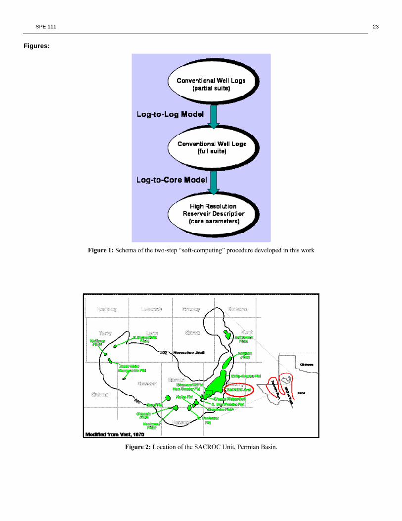
SPE 111 23

Figures:

Figure 1: Schema of the two-step “soft-computing” procedure developed in this work

Figure 2: Location of the SACROC Unit, Permian Basin.

SPE 111 24

Figure 3: General lithologic setting of SACROC Unit (modified from Raines, 2001).

Figure 4: Sacroc North Platform. Location of the characterized area.

SPE 111 25

Figure 5: Cross plot of log10(K0) vs log10(K90): well 11-15 in red; well 19-12 in blue; well 37-11 in green.

Figure 6: Cross plot of log10 (K0) vs porosity. Well 11-15 in red; well 19-12 in blue; well 37-11 in green.

SPE 111 26

Figure 7: Cross plots of window averaged log10(K0) vs. porosity. Well 11-15 in red; well 19-12 in blue; well 37-11 in green

Figure 8: Predicted core parameter using C1AA vs. predicted core parameter using C9. Porosity at left; log10(K0) at right. Well 11-15 in red; well 19-12 in blue; well 37-11 in green.

SPE 111 27

Figure 9: Tracks of predicted porosity values (two blue symbols) and predicted log10(K0) values (two green symbols).

Figure 10: Porosity and log10(K0) tracks for cored wells 11-15 and 19-12. Predicted porosity values in blue (two types); predicted log10(K0) values in green (two types), and actual core parameters in red.

6500 ft

6750 ft

7000 ft

6500 ft

6750 ft

7000 ft

Cored well 11-15Porosity tracks Permeability tracks

6500 ft

6750 ft

7000 ft

6500 ft

6750 ft

7000 ft

Cored well 19-12Porosity tracks Permeability tracks

6500 ft

6750 ft

7000 ft

6500 ft

6750 ft

7000 ft

Cored well 11-15Porosity tracks Permeability tracks

6500 ft

6750 ft

7000 ft

6500 ft

6750 ft

7000 ft

6500 ft

6750 ft

7000 ft

6500 ft

6750 ft

7000 ft

Cored well 11-15Porosity tracks Permeability tracks

Cored well 11-15Porosity tracks Permeability tracksPorosity tracks Permeability tracks

6500 ft

6750 ft

7000 ft

6500 ft

6750 ft

7000 ft

Cored well 19-12Porosity tracks Permeability tracks

6500 ft

6750 ft

7000 ft

6500 ft

6750 ft

7000 ft

6500 ft

6750 ft

7000 ft

6500 ft

6750 ft

7000 ft

Cored well 19-12Porosity tracks Permeability tracks

Cored well 19-12Porosity tracks Permeability tracksPorosity tracks Permeability tracks

SPE 111 28

Figure 11: AI_log (1st track), porosity (2nd track) and log10(K0) (3rd track) for testing hold-out cored well 11-15. Actual parameter values in red; predicted values in blue.

Figure 12: Cross plots of predicted vs. actual values for AI_log (left); porosity (center); log10(K0) (right). Ranges: AI_log [20, 60]; porosity [0.0, 0.3]; log10(K0) [-2.75, 2.75]

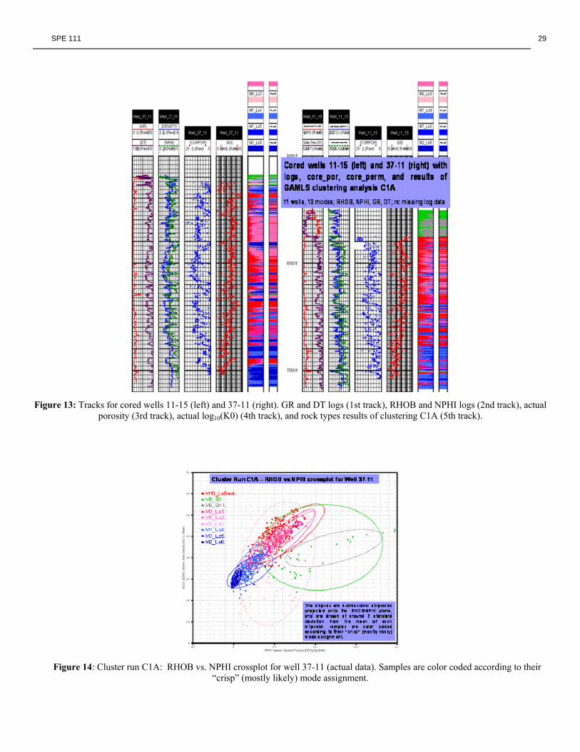
SPE 111 29

Figure 13: Tracks for cored wells 11-15 (left) and 37-11 (right). GR and DT logs (1st track), RHOB and NPHI logs (2nd track), actual porosity (3rd track), actual log10(K0) (4th track), and rock types results of clustering C1A (5th track).

Figure 14: Cluster run C1A: RHOB vs. NPHI crossplot for well 37-11 (actual data). Samples are color coded according to their “crisp” (mostly likely) mode assignment.

SPE 111 30

Figure 15: Tracks for the non cored well 33-15. Modes probabilistic representation (track 1); mode bed representation (track 2), core P&P estimates (tracks 3 and 4); RHOB (blue), NPHI (green), and AI_Log (orange) at track 5.

Figure 16: Cluster C1A, well 33-15 (no core data, RHOB & DT logs available). Predicted log10(K0) vs. predicted porosity for each of the modes (predictions using the "P&P_AI" method)

SPE 111 31

Figure 17: Comparison of realizations of cored well 37-11 from five different multi-well clustering runs.

Figure 18: Plane view of cross sections A-A’, B-B’, and C-C’ through central study area

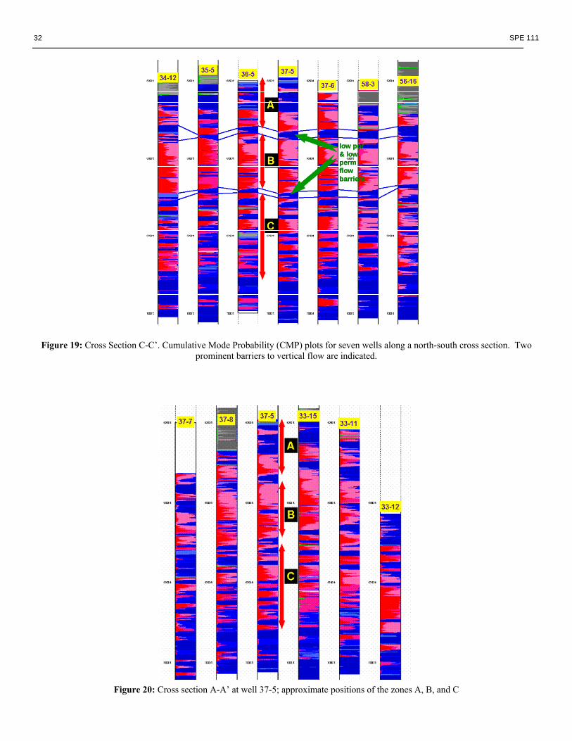
SPE 111 32

Figure 19: Cross Section C-C’. Cumulative Mode Probability (CMP) plots for seven wells along a north-south cross section. Two

prominent barriers to vertical flow are indicated.

Figure 20: Cross section A-A’ at well 37-5; approximate positions of the zones A, B, and C

low por & low perm flow barriers

low por & low perm flow barriers

low por & low perm flow barriers

SPE 111 33

Figure 21: Twelve wells of clustering run C1A oriented according to relative structural position using a prominent low RQ “bed” near the bottom of the studied interval. This “bed” is interpreted to be the base of sequence boundary “top C1” identified by Waite

(1993) and would represent a flooding surface.

Figure 22: Normalized porosity. Vertical experimental and model variograms.

SPE 111 34

Figure 23: Directional experimental variograms of normalized porosity. Directions: 0°, 30°, 45°, 60°, 90°, 120°, 135°, 150°.

Figure 24: Directional experimental variograms and fitted models. Left: N0°E; Right: N45°E.

Figure 25: Normalized log10(K0). Vertical experimental and model variograms.

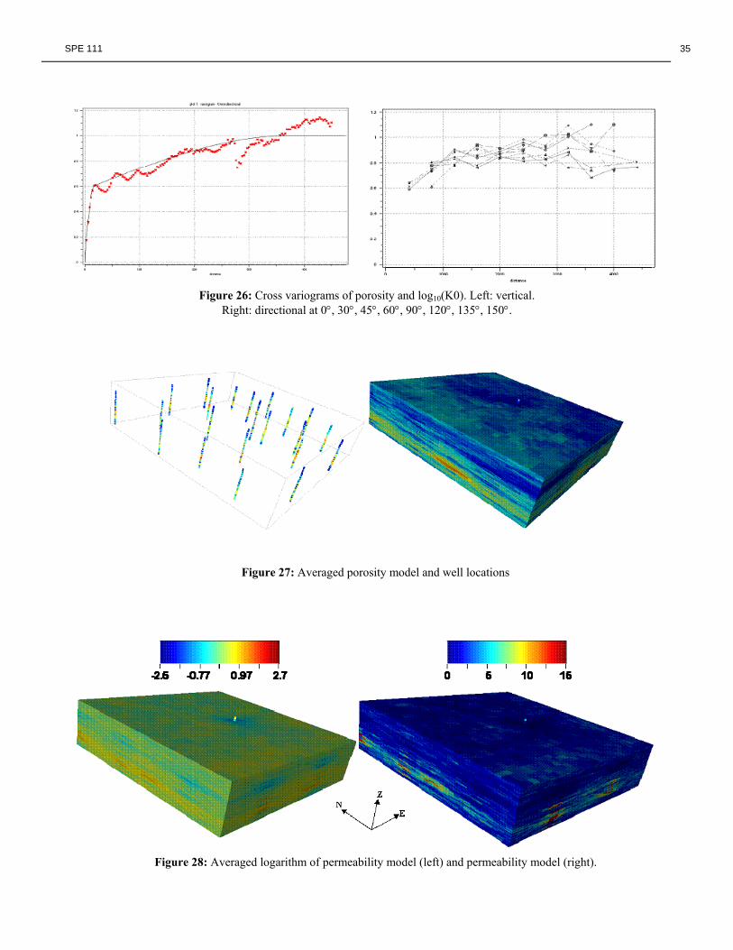
SPE 111 35

Figure 26: Cross variograms of porosity and log10(K0). Left: vertical. Right: directional at 0°, 30°, 45°, 60°, 90°, 120°, 135°, 150°.

Figure 27: Averaged porosity model and well locations

Figure 28: Averaged logarithm of permeability model (left) and permeability model (right).

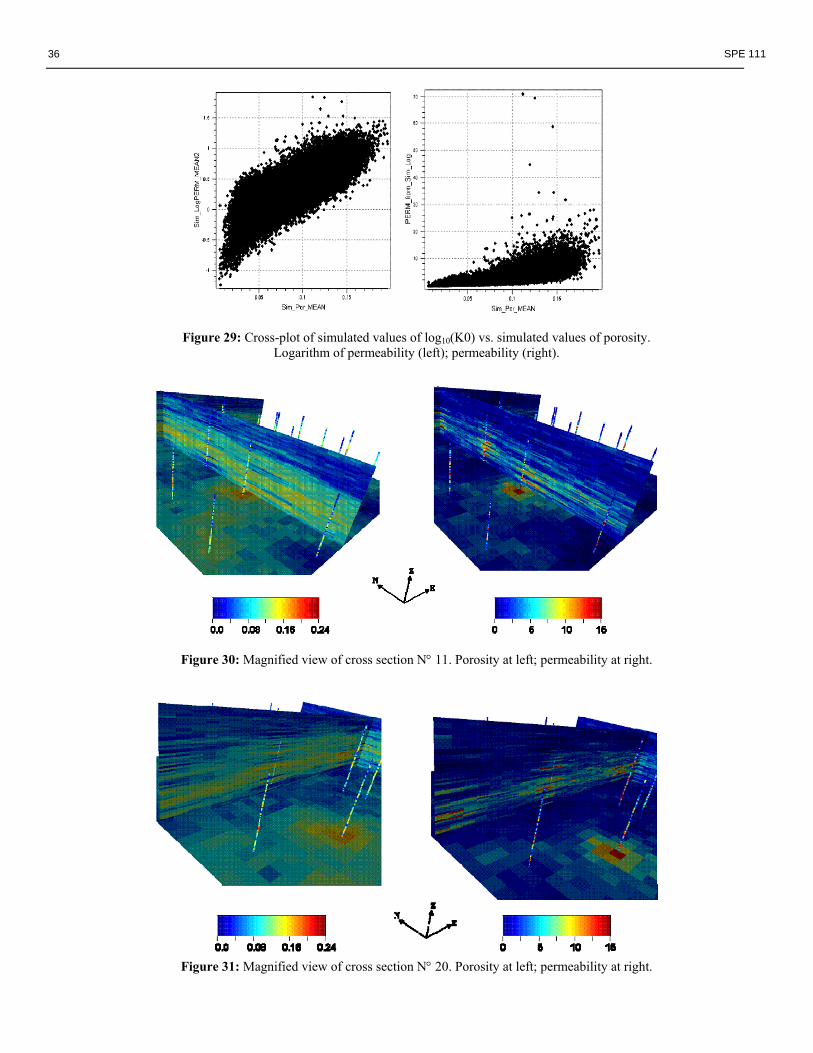
SPE 111 36

Figure 29: Cross-plot of simulated values of log10(K0) vs. simulated values of porosity. Logarithm of permeability (left); permeability (right).

Figure 30: Magnified view of cross section N° 11. Porosity at left; permeability at right.

Figure 31: Magnified view of cross section N° 20. Porosity at left; permeability at right.

SPE 111 37

Figure 32: Indicator maps based on a permeability threshold value of 2.74 md. Cross section N° 11 at left; cross section N° 20 at right.

SPE 111 38

Appendix A - Revisiting Permeability Predictions and Variation of K0, K90 and KV with Flow Units

Figure A-1: log10(K90) vs. log10(K0) for cored well 11-15 (left). Log10(K0) vs. log10(K0/K90) for cored well 11-15 (right). Samples colored according to “crisp” mode assignment from cluster C1A.

Figure A-2: Crossplot log10(KV) vs. log10(K0) for cored well 11-15. Samples colored according to “crisp” mode assignment from cluster C1A.

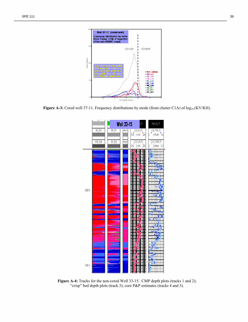
SPE 111 39

Figure A-3: Cored well 37-11. Frequency distributions by mode (from cluster C1A) of log10 (KV/KH).

Figure A-4: Tracks for the non-cored Well 33-15. CMP depth plots (tracks 1 and 2); “crisp” bed depth plots (track 3); core P&P estimates (tracks 4 and 5).

SPE 111 40

Figure A-5: Crossplot of C1C predicted porosity vs. actual core porosity using cored well 11-15 as a hold-out well. Flow unit colors from cluster C1C (left) and cluster C1A (right).

Figure A-6: Crossplot of C1C predicted log10(K0) vs. actual core log10(K0) for hold-out test cored wells 11-15 (left) and well 19-

12 (right). Flow unit colors are from cluster C1C.

SPE 111 41

Figure A-7: Frequency distributions for actual and predicted porosity (top), and actual and predicted log10(k0) (bottom). Well 11-15 (left); well 19-12 (right).

Figure A-8: log10 (K0) vs. [log10 (K0) −predicted log10 (K0)] for cored well 11-15. Samples colored according to “crisp” mode assignment from cluster C1A.