Spatiotemporal patterns of elephant poachingin south-eastern Kenya

John K. MaingiA,D, Joseph M. MukekaB, Daniel M. KyaleC and Robert M. MuasyaB

ADepartment of Geography, Miami University, Shideler Hall, Room 210, Oxford, OH 45056, USA.BKenya Wildlife Service Headquarters, PO Box 40241-00100, Nairobi, Kenya.CKenya Wildlife Service, Tsavo East National Park, PO Box 14, Voi, Kenya.DCorresponding author. Email: maingijk@muohio.edu

AbstractContext. Poaching of the African elephant for ivory had been on the increase since 1997 when the Convention on

InternationalTrade inEndangeredSpecies (CITES) allowedaone-off legal sale of ivoryby several southernAfrica countries.In Kenya, reports indicate continuous year-to-year increase in elephant poaching since 2003.

Aims. The goals of the study were to describe the temporal and spatial patterns of elephant poaching in south-easternKenya between 1990 and 2009, and examine relationships between observed patterns of poaching, and human andbiophysical variables. The study aimed to answer the following questions: (1) how has elephant poaching varied seasonallyand annually; (2) what are the spatial patterns of elephant poaching in the Tsavo Conservation Area (TCA); and (3) what arethe relationships between observed patterns of poaching and human and biophysical variables?

Methods. The study used elephant-poaching data and various GIS-data layers representing human and environmentalvariables to describe the spatial and temporal patterns of elephant poaching. The observed patterns were then related toenvironmental and anthropogenic variables using correlation and regression analyses.

Key results. Elephant poaching was clustered, with a majority of the poaching occurring in the dry season. Hotspots ofpoachingwere identified in areaswith higher densities of roads,waterholes, rivers and streams. TheTsavoEastNational Parkand the Tsavo National Park accounted for 53.7% and 44.8% of all poached elephants, respectively. The best predictors forelephant poachingwere density of elephants, condition of vegetation, proximity to ranger bases andoutposts, anddensities ofroads and rivers.

Conclusions. Predictor variables used in the study explained 61.5–78% of the total variability observed in elephantpoaching. The location of the hotspots suggests that human–wildlife conflicts in the areamaybe contributing to poaching andthat factors that quantify community attitudes towards elephant conservation may provide additional explanation forobserved poaching patterns.

Implications. The poaching hotpots identified can be a used as starting point by the Kenya Wildlife Service (KWS) tobegin implementing measures that ensure local-community support for conservation, whereas on other hotspots, it will benecessary to beef-up anti-poaching activities. There is a need for Kenya to legislate new anti-poaching laws that are a muchmore effective deterrence to poaching than currently exist.

Received 25 January 2011, accepted 4 January 2012, published online 12 April 2012

Introduction

The decline in the population of the African elephant (Loxodontaafricana) from 1.3million to 600 000 between 1979 and 1987has been attributed mainly to indiscriminate poaching for ivory(Douglas-Hamilton 1987). In Kenya, the population of elephantsfell from ~130 000 in 1973 to 16 000 in 1989 (Cohn 1990). Thisincrease in poaching activity paralleled the dramatic increases inthe price of ivory, with the price of a kilogram of uncarved ivoryin Kenya worth approximately $5.50 in 1969, $75 in 1978 and$198 in 1989 (Messer 2000). The drastic decline in the populationof elephants prompted the CITES to remove the African elephantfrom Appendix II to Appendix I, effectively banning tradein ivory (Burton 1999). Appendix I lists species threatened

with extinction and prohibits commercial trade, while tightlycontrolling other trade. Appendix II lists those species notnecessarily threatened with extinction but in which trade mustbe controlled to ensure their survival (CITES 2009). The ivorytrade ban was contested by several southern African states thathad thriving elephant populations, and thus viewed ivory sales asa means to fund wildlife conservation and protect habitat.

In 1997, CITES decided to down-list elephant populationsin Botswana, Namibia and Zimbabwe to Appendix II, thuspermitting a sell-off of 50 t of stockpiled ivory to Japan (Stiles2004). Again in 2002, CITES gave conditional approval toBotswana, Namibia and South Africa to sell 60 t of stock-piledivory (Stiles 2004). It was not until 2007 that CITES member

CSIRO PUBLISHING

Wildlife Researchhttp://dx.doi.org/10.1071/WR11017

Journal compilation � CSIRO 2012 www.publish.csiro.au/journals/wr

countries gave full support to the auction (Lemieux and Clarke2009). In 2008, CITES approved sale of 108 t of ivory to Japanfrom southern African countries (Santiapillai 2009). ManyAfrican countries opposed this sale because they believed itwould provide a loophole for poached ivory to enter theinternational market once again (Lemieux and Clarke 2009).

The idea that one-off sale of ivory results in increasedpoaching is under intense debate. Stiles (2004) argued thatthere is little evidence to support claims that the 1999 ivoryauctions by southern Africa countries resulted in increasedpoaching. Stiles (2004) attributed levels of poaching in anycountry to wildlife management practices in place, lawenforcement and corruption, rather than decisions on ivorytrade by CITES. By using DNA evidence, Wasser et al.(2007) found that some ivory seized in Asia originated fromAfrican countries not taking part in CITES one-off ivory saleand suggested that the ivory had been shipped across bordersbefore being exported to Asia. Wasser et al. (2007) claimedthere was a clear link between one-off ivory sales and the risein poaching in Africa. Bulte et al. (2007) also found evidenceof increased elephant poaching at the local level in bothZimbabwe and Kenya, following the one-off sale of ivory;however, these authors concluded that the increase was smalland most probably short-lived. A recent study by Lemieux andClarke (2009) examined changes in elephant populationsbetween 1989 and 2007 for 36 of the 37 elephant range statesin Africa and concluded that the ivory ban helped increase theoverall number of elephants inAfrica by~140 000. In all, 18 of 36countries showed increases in elephant numbers since the 1989ban, and the ban slowed down the loss of elephants in others.Lemieux and Clarke (2009) also identified 17 countries withdeclining elephant populations over the period, with CentralAfrica losing 130 000 elephants in the post-ban years.

Recent reports from Kenya indicate continuous year-to-yearincrease in the proportion of illegally killed elephants since2003 (Douglas-Hamilton 2009). The current study examinesthe temporal and spatial patterns of elephant poaching in theTCA for the period 1990–2009, and explores relationshipsbetween observed patterns of elephant poaching, and humanand biophysical variables.

Most African countries have laws that outlaw the killing ofelephants within protected areas; however, in reality, the lawsare poorly enforced. This lack of enforcement is attributed to avariety of reasons, including underfunding, corruption andinadequate equipment for law enforcement (Simons andKreuter 1989). Leader-Williams (1994) put the minimum costof conserving elephants during a time of intensive poaching inLuangwa Valley Zambia at approximately US$215 per km2 in1981 values. Barnes (1996) estimated the cost of conservingelephants in Botswana during a surge in poaching at an inflation-adjusted rate of US$246 per km2. In another study, Jachmannand Billiouw (1997) estimated that there should be a minimumof one park ranger per 24 km2 of wildlife reserve if effectivepatrolling and policing is to be realised. Kenya, like many othersub-Saharan African countries, is unable to meet these costs andthus cannot afford adequate protection of wildlife from poachingwithin national parks and reserves. The Kenya Wildlife Service(KWS), like most wildlife departments in sub-Saharan Africa,is understaffed with approximately one ranger per 100 km2 of

wildlife reserve. It is therefore important to explore strategiesthat will result in a more efficient deployment of the scarceresources within national parks and reserves. An examinationof spatial and temporal patterns of elephant mortality attributedto poaching within protected areas may provide importantinsights about areas that are most vulnerable to poaching andthus help guide a more effective policing of the parks andreserves.

The present study draws on previous research that soughtto explain the geographic variation in the rate of crime. At theglobal scale, a major perspective used to explain crime is basedon factors that increase the motivation to commit crime, andthose that enhance the opportunity for criminal activity (VanDijk 1994). Cohen and Felson (1979) came up with the conceptof distance decay, which suggests that most offences occurrelatively close to the domicile of a local offender. Thedistance-decay concept implies that crimes will tend to clusterwhere opportunities and motivated offenders are plentiful,and guardianship is missing or weak. In the case of elephantpoaching, we can expect poaching activity to be intense whereelephants are most abundant and where transportation of thepoached ivory directly to the ivory traders or through middlemenis easiest, because this provides the poacher with the highestreturn on effort. Likewise, we can expect poaching activityto be tempered by the poacher’s fear of detection by gamerangers and law enforcement. Indeed, Milner-Gulland andLeader-Williams (1992) found that the probability of capturewas a highly significant factor in the poacher’s decision tohunt black rhinos and elephants in the Luangwa Valley inZambia.

Several studies have explored relationships among elephantabundances, environmental variables and human factors.Several of these studies identified distance to water as theprimary environmental factor influencing the density ofelephant population at the local level (Western 1975;Verlinden and Gavor 1998; Redfern et al. 2003). In theCongo Basin, Blake et al. (2008) found that the abundance ofmany mammal species increased with distance from roadsbecause of hunting pressure.

Several studies looking at relationships between elephantsand vegetation have successfully utilised satellite-derivedvegetation indices such as the normalised difference vegetationindex (NDVI) and the enhanced vegetation index (EVI) asproxies for vegetation productivity (e.g. Chamaillé-Jammeset al. 2007; Hien et al. 2007; Loarie et al. 2009). MODIS EVIhas been shown to be well correlated with green leaf area index(LAI), biomass, canopy cover and the fraction of absorbedphotosynthetically active radiation (Gao et al. 2000) and isless sensitive to atmospheric aerosols and soil reflectance thanthe more commonly used normalised difference vegetation index(Jiang et al. 2008).

The TCA has the highest population of elephants, and thehighest reported incidences of elephant poaching in Kenya.Anti-poaching patrols in the TCA are particularly challengingbecause of limited resources, and the expansive area of the parkthat limits the effectiveness of patrols by park rangers. In thepresent study, we use GIS to describe poaching-inducedelephant-mortality patterns, and investigate biophysical andhuman factors associated with observed elephant-mortality

B Wildlife Research J. K. Maingi et al.

patterns. Such information would be useful in guiding thedeployment of policing resources throughout the park. Thestudy aims to answer the following questions: (1) how haselephant poaching varied seasonally and annually; (2) what arethe spatial patterns of elephant poaching in theTCAandwhere arethe poaching hotspots; (3) what are the relationships betweenobservedpatterns of poaching andanthropogenic andbiophysicalvariables?

Materials and methodsStudy site

The study area described as the TCA is predominantly lowlandsavannah, consisting of three national parks, and two nationalreserves (Fig. 1). The TCA covers an area of ~23 158 km2 andincludes the Tsavo East National Park (TENP), the Tsavo WestNational Park (TWNP), the Chyulu Hills National Park (CHNP),

38° E 39° E

-2° S

-3° S

-4° S

N

Fig. 1. Location of Tsavo Conservation Area (TCA) in south-eastern Kenya.

Elephant poaching in Tsavo, Kenya Wildlife Research C

the South Kitui National Reserve (SKNR) and the Ngai NdethyaNational Reserve (NNNR). Elevation in the park, as revealed bya 30-m digital elevationmodel (DEM), increases from south-eastto north-west, from 150m above sea level in parts of the TENPto ~2100m in the CHNP. The climate of the area is semiarid,with the long rains occurring between March and May, andthe short rains occurring between November and December.The wet season is therefore considered to be in March–Mayand November–December, and the dry season is in January–February and June–October. Rainfall varies between 100mm to1200mm per year and appears to closely follow elevation in asouth-east to north-west direction (Mukeka 2010). The mainsource of permanent water in TCA is the Galana River and itstributaries, the Athi River and the Tsavo River. Seasonal sourcesof water include the Tiva and Voi rivers, the Aruba Dam, severalswamps and numerous scattered ponds (Fig. 1).

Vegetation in the TCA is dominated by Acacia–Commiphorasavanna. The term savanna refers to varying densities of trees andshrubs, fromopenplains towoodlandsand shrub thickets (Gillson2004). TheAcacia–Commiphora vegetation in the TCA includes23 species of Acacia and 11 species of Commiphora and otherspecies such asGrewia spp,Lannea spp,Newtonia hildebrandtii,Premna resinosa, Salvadora persica, Terminalia spp, Bosciaspp,Cadaba spp. andMaerua spp. There are large trees scatteredwithin the ecosystem, including Adansonia digitata, Balanitesaegyptica, Delonix elata, Kigelia Africana and Melia volkensii(Gillson2004;Greenway1969).Vegetation is generally denser inthe north-western part of the park and lighter in the eastern part,corresponding to the rainfall gradient.

Data layersDatasets used in the present study and their sources are shown inTable 1. The list does not include GIS layers derived from thesedatasets. A 30-m DEM for the TCAwas obtained by mosaickingASTERglobal digital elevationmodel (GDEM)datadownloadedfrom theMinistry of EconomyTrade and Industry (METI), Japan

(METI andNASA2009). TheDEMwasused to obtain elevationsand derive slopes. Roads, water holes and rivers in the study areawere obtained by digitising a mosaic of Landsat TM and ETM+images downloaded from the US Geological Survey, and alsofrom digitising 1 : 50 000 topographic maps obtained fromDepartment of Surveys, Kenya. Vector GIS data includinglocations of ranger patrol bases and outposts, park gates andheadquarters, park boundaries, and an MS Excel spreadsheetcontaining elephant mortality data were obtained from theKWS. EVI images produced from the moderate resolutionimaging spectrometer (MODIS) on-board NASA’s TERRAsatellite were also available for the study. The MODIS product(MOD13Q) is a 16-day composite of highest-quality pixels fromdaily images available at a spatial resolution of 250m.Therewere23 EVI image composites per year for a total of 184 images overthe period 2001–2008. The MODIS EVI images weredownloaded from the USGS Land Processes DistributedActive Archive Center (LP DAAC). We calculated a meanEVI and a standard deviation EVI image from the 184 MODISEVI images. The two calculated images would serve as a proxyfor vegetation condition in the TCA for the period 2001–2008.A land-cover map, prepared by Mukeka (2010) from LandsatTM and ETM+ data was also available for the study.

Data analysis

Elephant-mortality data covered the period from 1 January 1990to 31 December 2009 and included geographic coordinates ofareas where elephant carcasses were found, names of thelocations, and date and cause of elephant mortality. The Excelspreadsheet provided by KWS had 430 listed locations ofelephant mortality in the study area and surroundingcommunal lands. Of these locations, 210 points fell inside theTCA. Some of the 210 points of elephantmortality hadmore thanone elephant carcass recorded, bringing the total number ofelephants poached in the TCA between 1990 and 2009 to 268.There were 35 additional entries of poaching incidences in thedatabase but these were excluded from analyses because theylacked geographic coordinates. Although the excluded recordsincluded the names of the locationswhere the poaching occurred,the names were too ambiguous to be used to approximate thepoaching locations.

Mortality dates for recorded elephant carcasses weretranslated to season categories based on rainfall distribution inthe study area. The November–December and March–Mayperiods were categorised as ‘wet season’, the June–Octoberperiod as ‘dry season’, and the January–February period as‘short-dry season’. Elephant mortality data were thenconverted to a GIS shapefile in ArcGIS (ESRI 2011). A 10-kmbuffer of the TCA was generated and used to clip elephant-mortality data to the buffer area. The 10-km buffer was deemedsufficient to reduce edge effects during point pattern analysis(Griffith 1985). The spatial extents of subsequent datasetsgenerated for the present study were all clipped to the 10-kmbuffer. The elephant-mortality shapefile included all causes ofelephant mortality and was therefore queried to extract andcreate a new elephant-mortality shapefile attributed topoaching. This shapefile was queried and used to describe thetemporal and spatial patterns of elephant poaching across all

Table 1. Sources of data used in current studyEVI, enhanced vegetation index

Data Source

30-m digital elevationmodel (DEM)

Ministry of Economy Trade and Industry(METI), Japan and NASA

Land-cover map Derived from Landsat TM and ETM+and prepared by Mukeka (2010)

Roads and rivers Digitised from topographic maps andLandsat ETM+ images

Waterholes Kenya Wildlife Service (KWS)Management points

(park offices, gates,lodges, patrol basesand outposts)

Kenya Wildlife Service (KWS)

Settlements Digitised from 1 : 50 000 topographicmaps

MODIS 16-day EVIcomposite images

Downloaded from USGS’s LandProcesses Distributed

Active Archive Center (LP DAAC)Elephant-mortality data Kenya Wildlife Service (KWS)

D Wildlife Research J. K. Maingi et al.

seasons, and in the wet and in the dry seasons. A detaileddescription of techniques used to analyse spatial patterns ofpoaching is included below.

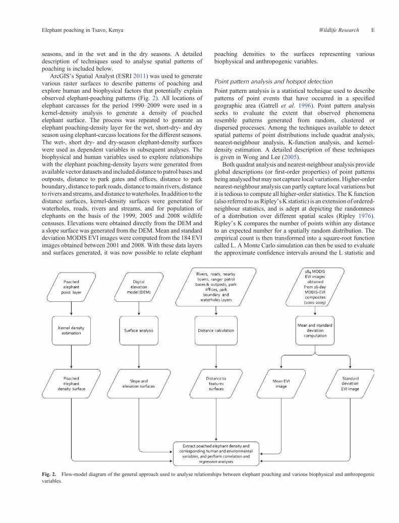
ArcGIS’s Spatial Analyst (ESRI 2011) was used to generatevarious raster surfaces to describe patterns of poaching andexplore human and biophysical factors that potentially explainobserved elephant-poaching patterns (Fig. 2). All locations ofelephant carcasses for the period 1990–2009 were used in akernel-density analysis to generate a density of poachedelephant surface. The process was repeated to generate anelephant poaching-density layer for the wet, short-dry- and dryseason using elephant-carcass locations for the different seasons.The wet-, short dry- and dry-season elephant-density surfaceswere used as dependent variables in subsequent analyses. Thebiophysical and human variables used to explore relationshipswith the elephant poaching-density layers were generated fromavailable vector datasets and included distance to patrol bases andoutposts, distance to park gates and offices, distance to parkboundary, distance to park roads, distance tomain rivers, distanceto rivers and streams, anddistance towaterholes. In addition to thedistance surfaces, kernel-density surfaces were generated forwaterholes, roads, rivers and streams, and for population ofelephants on the basis of the 1999, 2005 and 2008 wildlifecensuses. Elevations were obtained directly from the DEM anda slope surface was generated from the DEM.Mean and standarddeviation MODIS EVI images were computed from the 184 EVIimages obtained between 2001 and 2008. With these data layersand surfaces generated, it was now possible to relate elephant

poaching densities to the surfaces representing variousbiophysical and anthropogenic variables.

Point pattern analysis and hotspot detectionPoint pattern analysis is a statistical technique used to describepatterns of point events that have occurred in a specifiedgeographic area (Gatrell et al. 1996). Point pattern analysisseeks to evaluate the extent that observed phenomenaresemble patterns generated from random, clustered ordispersed processes. Among the techniques available to detectspatial patterns of point distributions include quadrat analysis,nearest-neighbour analysis, K-function analysis, and kernel-density estimation. A detailed description of these techniquesis given in Wong and Lee (2005).

Both quadrat analysis and nearest-neighbour analysis provideglobal descriptions (or first-order properties) of point patternsbeing analysed butmaynot capture local variations.Higher-ordernearest-neighbour analysis can partly capture local variations butit is tedious to compute all higher-order statistics. The K function(also referred to asRipley’sK statistic) is an extension of ordered-neighbour statistics, and is adept at depicting the randomnessof a distribution over different spatial scales (Ripley 1976).Ripley’s K compares the number of points within any distanceto an expected number for a spatially random distribution. Theempirical count is then transformed into a square-root functioncalled L. A Monte Carlo simulation can then be used to evaluatethe approximate confidence intervals around the L statistic and

Fig. 2. Flow-model diagram of the general approach used to analyse relationships between elephant poaching and various biophysical and anthropogenicvariables.

Elephant poaching in Tsavo, Kenya Wildlife Research E

the L statistic calculated for randomly assigned data. Because theK function is also subject to the boundary problem, it is necessaryto adjust for the boundary effect by including a weighting(Bailey and Gatrell 1995). The real value of K-functionanalysis is its ability to explore the spatial point pattern overthe entire scale of the study region while including all points anddistances between all points, and not just nearest neighbours(Wong and Lee 2005).

The kernel-density transformation is one of the most usefulin applied GIS and provides a very good way of visualisingpoint pattern to detect hotspots (O’Sullivan and Unwin 2003).Kernel-density estimation provides a map of estimates of thelocal intensity of any spatial process from a set of observedoccurrences (Bailey andGatrell 1995).Because kernel estimationresults in a continuous surface, it provides a means to link pointfeatures to other geographic data (O’Sullivan and Unwin 2003).The degree of smoothness of the output surface is determined bythe bandwidth (the length of the search radius within which thekernel exerts its influence) used in the analysis.A large bandwidthresults in a large amount of smoothing and produces a fluidmap with low intensity levels. A small bandwidth results in lesssmoothing and a spiky map, with local variations in intensitylevels (Anselin et al. 2000) The ability of Kernel estimation totransformspatial point patterns into a smooth imagemakes it idealfor visualising hotspots and potential hotspots as areas of highdensity.

Relationships between elephant poaching densityand biophysical and human variables

Relationships between elephant poaching and variousbiophysical and human factors were examined throughSpearman rank correlation analysis. The biophysical andhuman factors included (1) distance to park-management units(park offices, park gates, park ranger patrol bases and outposts),(2) distance to human influences (includes park offices, parkgates, park ranger patrol bases and outposts, and lodges),(3) distance to ranger patrol bases and outposts, (4) densityand distance to roads, (5) distance to settlements, (6) densityand distance to rivers and streams, (7) density and distance towaterholes, (8) elevation, (9) slope, (10) mean of 16-dayMODISEVI composite images, and (11) standard deviation of 16-dayMODIS EVI composite images.

ArcGIS’ Spatial Analyst kernel-density function was usedto generate distance surfaces to ranger patrol bases, park-management units, park roads, rivers and streams, andwaterholes. In addition to the distance surfaces, density surfaceswere generated for overall poaching, dry-season poaching, shortdry-season poaching, wet-season poaching, water points, riversand streams, and roads. This kernel-density function requires abandwidth and cell size to be specified. We used ArcGIS’sincremental spatial autocorrelation tool to determine the optimalspatial scale for analysis. The toolmeasures spatial autocorrelationof point data at incremental distances and creates a graph of thosedistances and their z-scores. Peaks in the output graph indicatedistances where clustering is most pronounced (ESRI 2011).A bandwidth of 50km was chosen because this is the distancethat correspondedwith the highest degree of clustering in poachedelephants. A cell size of 250m was selected because it coincided

with the resolution of theMODISEVIdata, andbecause amajorityof poached-elephant carcass locations obtained before 2006 wereonly approximate, having been interpreted from topographicmapsrather than acquired using GPS receivers.

Once poaching-density surfaces and surfaces correspondingto the various biophysical and human variables were generated,data were extracted from the surfaces to analyse relationshipsamong the layers. We used the 210 elephant-poaching locationsto extract data from various layers and implemented theSpearman rank correlation analysis because the data werenot normally distributed. Multiple regressions to predict therelationships between elephant-poaching surfaces and thevarious biophysical and human variable surfaces required ourdata to be normally distributed and to be spatially independent.The data extracted from the 210 locations showed high spatialautocorrelation and therefore invalidated many of the parametricstatistical analyses available. We, therefore, chose to extract datafrom the layers usinga set of randompoints spacedwidely enoughto reduce spatial dependency. We determined the minimumdistance needed to be maintained among the random locationsby running Moran’s I autocorrelation analysis (Moran 1950;Sokal and Oden 1978). This analysis indicated that spatialautocorrelation in poaching density was greatly reduced whengenerated random points were spaced at least 5 km apart. We,therefore, used this minimum spacing distance to generaterandom locations that we could use to extract data from thevarious surfaces for regression analyses.

Prior to multiple-regression analyses, predictor variablesidentified earlier as significantly correlated with elephant-poaching density were tested for normality using theShapiro–Wilk normality test. The Shapiro–Wilk test isrecommended over the Kolmogorov–Smirnov test whensample sizes are small, i.e. less than 2000 (Kaltenbach 2012).The non-normally distributed variables were normalised usingdata transformation procedures such as reciprocal, logarithmicand power transformations (Boslaugh and Watters 2008).Following data normalisation, a subset of explanatoryvariables was selected for input in multiple regressions afterfirst screening them for multi-collinearity using the Pearson’sproduct–moment correlation. Next, we generated multipleregression models to predict poaching density and used thebest-subsets method (Hosmer et al. 1989) and chose modelswith the lowest Akaike’s information criterion (Burnham et al.2002). The residuals of each regression model were thenevaluated for autocorrelation using the Durbin–Watson test.

Results

Spatiotemporal patterns of elephant mortality

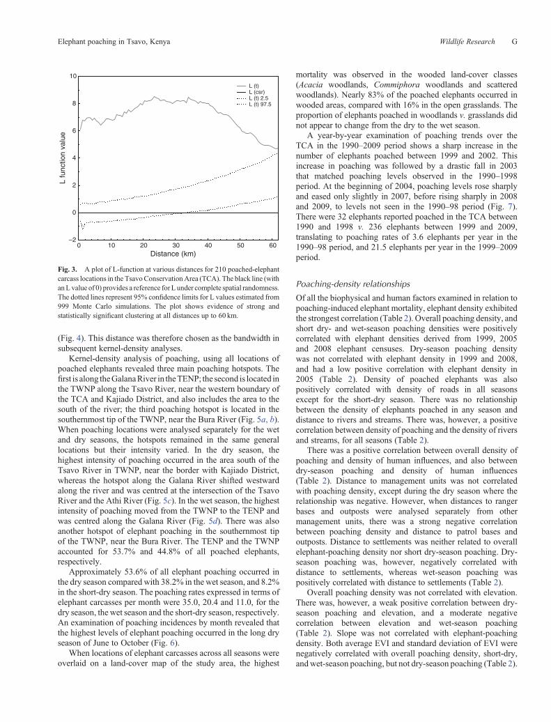
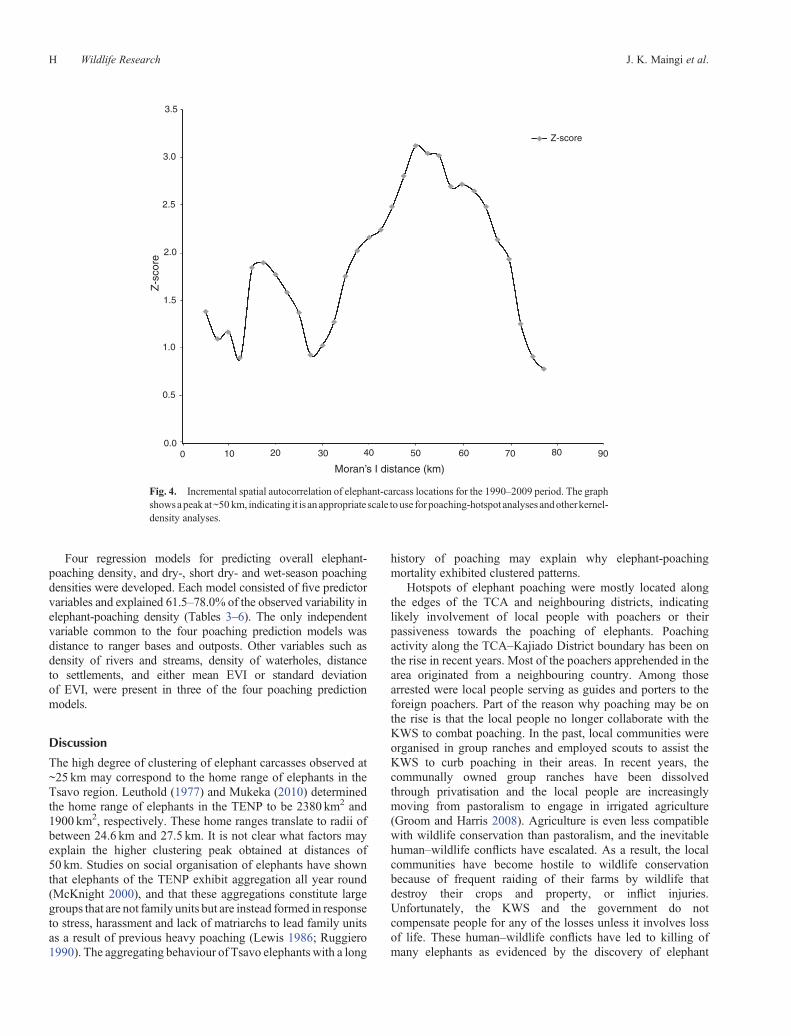
Results from Ripley’s K-function analysis revealed thatpoaching-induced elephant mortality in the TCA displayedsignificantly clustered patterns (Fig. 3). Values of L greaterthan the 95% confidence intervals indicate clusteredconcentration of elephant carcasses. In this case, poached-elephant carcasses were clustered at all distances examined upto 60 km. An analysis of poached-elephant locations usingArcGIS’s incremental spatial autocorrelation tool indicatedthat maximum clustering occurred at a distance of ~50 km

F Wildlife Research J. K. Maingi et al.

(Fig. 4). This distance was therefore chosen as the bandwidth insubsequent kernel-density analyses.

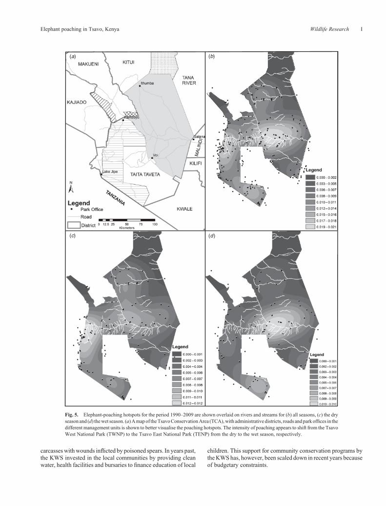
Kernel-density analysis of poaching, using all locations ofpoached elephants revealed three main poaching hotspots. Thefirst is along theGalanaRiver in theTENP; the second is located inthe TWNP along the Tsavo River, near the western boundary ofthe TCA and Kajiado District, and also includes the area to thesouth of the river; the third poaching hotspot is located in thesouthernmost tip of the TWNP, near the Bura River (Fig. 5a, b).When poaching locations were analysed separately for the wetand dry seasons, the hotspots remained in the same generallocations but their intensity varied. In the dry season, thehighest intensity of poaching occurred in the area south of theTsavo River in TWNP, near the border with Kajiado District,whereas the hotspot along the Galana River shifted westwardalong the river and was centred at the intersection of the TsavoRiver and the Athi River (Fig. 5c). In the wet season, the highestintensity of poaching moved from the TWNP to the TENP andwas centred along the Galana River (Fig. 5d). There was alsoanother hotspot of elephant poaching in the southernmost tipof the TWNP, near the Bura River. The TENP and the TWNPaccounted for 53.7% and 44.8% of all poached elephants,respectively.

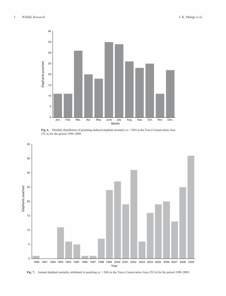
Approximately 53.6% of all elephant poaching occurred inthe dry season compared with 38.2% in the wet season, and 8.2%in the short-dry season. The poaching rates expressed in terms ofelephant carcasses per month were 35.0, 20.4 and 11.0, for thedry season, the wet season and the short-dry season, respectively.An examination of poaching incidences by month revealed thatthe highest levels of elephant poaching occurred in the long dryseason of June to October (Fig. 6).

When locations of elephant carcasses across all seasons wereoverlaid on a land-cover map of the study area, the highest

mortality was observed in the wooded land-cover classes(Acacia woodlands, Commiphora woodlands and scatteredwoodlands). Nearly 83% of the poached elephants occurred inwooded areas, compared with 16% in the open grasslands. Theproportion of elephants poached in woodlands v. grasslands didnot appear to change from the dry to the wet season.

A year-by-year examination of poaching trends over theTCA in the 1990–2009 period shows a sharp increase in thenumber of elephants poached between 1999 and 2002. Thisincrease in poaching was followed by a drastic fall in 2003that matched poaching levels observed in the 1990–1998period. At the beginning of 2004, poaching levels rose sharplyand eased only slightly in 2007, before rising sharply in 2008and 2009, to levels not seen in the 1990–98 period (Fig. 7).There were 32 elephants reported poached in the TCA between1990 and 1998 v. 236 elephants between 1999 and 2009,translating to poaching rates of 3.6 elephants per year in the1990–98 period, and 21.5 elephants per year in the 1999–2009period.

Poaching-density relationships

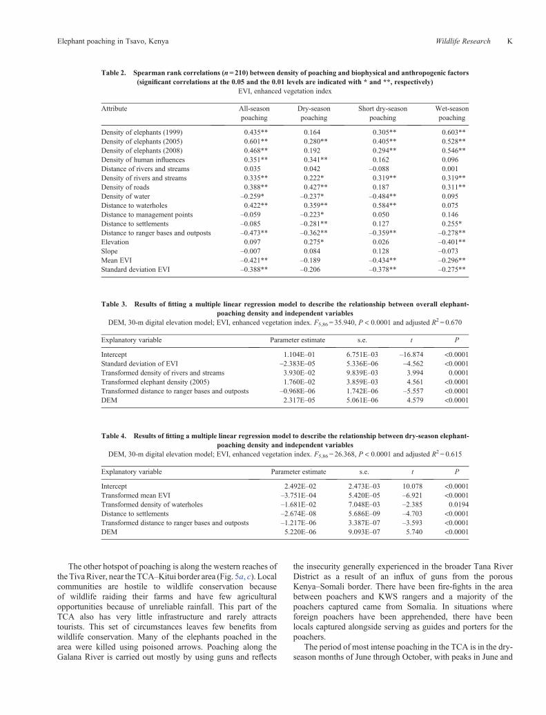
Of all the biophysical and human factors examined in relation topoaching-induced elephant mortality, elephant density exhibitedthe strongest correlation (Table 2). Overall poaching density, andshort dry- and wet-season poaching densities were positivelycorrelated with elephant densities derived from 1999, 2005and 2008 elephant censuses. Dry-season poaching densitywas not correlated with elephant density in 1999 and 2008,and had a low positive correlation with elephant density in2005 (Table 2). Density of poached elephants was alsopositively correlated with density of roads in all seasonsexcept for the short-dry season. There was no relationshipbetween the density of elephants poached in any season anddistance to rivers and streams. There was, however, a positivecorrelation between density of poaching and the density of riversand streams, for all seasons (Table 2).

There was a positive correlation between overall density ofpoaching and density of human influences, and also betweendry-season poaching and density of human influences(Table 2). Distance to management units was not correlatedwith poaching density, except during the dry season where therelationship was negative. However, when distances to rangerbases and outposts were analysed separately from othermanagement units, there was a strong negative correlationbetween poaching density and distance to patrol bases andoutposts. Distance to settlements was neither related to overallelephant-poaching density nor short dry-season poaching. Dry-season poaching was, however, negatively correlated withdistance to settlements, whereas wet-season poaching waspositively correlated with distance to settlements (Table 2).

Overall poaching density was not correlated with elevation.There was, however, a weak positive correlation between dry-season poaching and elevation, and a moderate negativecorrelation between elevation and wet-season poaching(Table 2). Slope was not correlated with elephant-poachingdensity. Both average EVI and standard deviation of EVI werenegatively correlated with overall poaching density, short-dry,andwet-season poaching, but not dry-season poaching (Table 2).

0 10 20 30 40 50 60Distance (km)

–2

0

2

4

6

8

10

L fu

nctio

n va

lue

L (t)L (csr)L (t) 2.5L (t) 97.5

Fig. 3. A plot of L-function at various distances for 210 poached-elephantcarcass locations in the TsavoConservationArea (TCA). The black line (withanL value of 0) provides a reference for L under complete spatial randomness.The dotted lines represent 95% confidence limits for L values estimated from999 Monte Carlo simulations. The plot shows evidence of strong andstatistically significant clustering at all distances up to 60 km.

Elephant poaching in Tsavo, Kenya Wildlife Research G

Four regression models for predicting overall elephant-poaching density, and dry-, short dry- and wet-season poachingdensities were developed. Each model consisted of five predictorvariables and explained 61.5–78.0% of the observed variability inelephant-poaching density (Tables 3–6). The only independentvariable common to the four poaching prediction models wasdistance to ranger bases and outposts. Other variables such asdensity of rivers and streams, density of waterholes, distanceto settlements, and either mean EVI or standard deviationof EVI, were present in three of the four poaching predictionmodels.

Discussion

The high degree of clustering of elephant carcasses observed at~25 km may correspond to the home range of elephants in theTsavo region. Leuthold (1977) and Mukeka (2010) determinedthe home range of elephants in the TENP to be 2380 km2 and1900 km2, respectively. These home ranges translate to radii ofbetween 24.6 km and 27.5 km. It is not clear what factors mayexplain the higher clustering peak obtained at distances of50 km. Studies on social organisation of elephants have shownthat elephants of the TENP exhibit aggregation all year round(McKnight 2000), and that these aggregations constitute largegroups that are not family units but are instead formed in responseto stress, harassment and lack of matriarchs to lead family unitsas a result of previous heavy poaching (Lewis 1986; Ruggiero1990). The aggregating behaviour of Tsavo elephants with a long

history of poaching may explain why elephant-poachingmortality exhibited clustered patterns.

Hotspots of elephant poaching were mostly located alongthe edges of the TCA and neighbouring districts, indicatinglikely involvement of local people with poachers or theirpassiveness towards the poaching of elephants. Poachingactivity along the TCA–Kajiado District boundary has been onthe rise in recent years. Most of the poachers apprehended in thearea originated from a neighbouring country. Among thosearrested were local people serving as guides and porters to theforeign poachers. Part of the reason why poaching may be onthe rise is that the local people no longer collaborate with theKWS to combat poaching. In the past, local communities wereorganised in group ranches and employed scouts to assist theKWS to curb poaching in their areas. In recent years, thecommunally owned group ranches have been dissolvedthrough privatisation and the local people are increasinglymoving from pastoralism to engage in irrigated agriculture(Groom and Harris 2008). Agriculture is even less compatiblewith wildlife conservation than pastoralism, and the inevitablehuman–wildlife conflicts have escalated. As a result, the localcommunities have become hostile to wildlife conservationbecause of frequent raiding of their farms by wildlife thatdestroy their crops and property, or inflict injuries.Unfortunately, the KWS and the government do notcompensate people for any of the losses unless it involves lossof life. These human–wildlife conflicts have led to killing ofmany elephants as evidenced by the discovery of elephant

3.5

Z-score

3.0

2.5

2.0

1.5

1.0

0.5

0.00 10 20 30 40

Moran’s I distance (km)

Z-s

core

50 60 70 80 90

Fig. 4. Incremental spatial autocorrelation of elephant-carcass locations for the 1990–2009 period. The graphshowsapeakat~50 km, indicating it is anappropriate scale touse forpoaching-hotspot analyses andotherkernel-density analyses.

H Wildlife Research J. K. Maingi et al.

carcasseswithwounds inflicted by poisoned spears. In years past,the KWS invested in the local communities by providing cleanwater, health facilities and bursaries to finance education of local

children. This support for community conservation programs bytheKWShas, however, been scaled down in recent years becauseof budgetary constraints.

(a) (b)

(c) (d )

Fig. 5. Elephant-poaching hotspots for the period 1990–2009 are shown overlaid on rivers and streams for (b) all seasons, (c) the dryseasonand (d) thewet season. (a)Amapof theTsavoConservationArea (TCA),with administrative districts, roads andparkoffices in thedifferent management units is shown to better visualise the poaching hotspots. The intensity of poaching appears to shift from the TsavoWest National Park (TWNP) to the Tsavo East National Park (TENP) from the dry to the wet season, respectively.

Elephant poaching in Tsavo, Kenya Wildlife Research I

0

5

10

15

20

25

30

35

40

Jan. Feb. Mar. Apr. May June July Aug. Sep. Oct. Nov. Dec.

Ele

phan

ts p

oach

ed

Month

Fig. 6. Monthly distribution of poaching-induced elephant mortality (n = 268) in the Tsavo Conservation Area(TCA) for the period 1990–2009.

0

5

10

15

20

25

30

35

40

1990 1991 1992 1993 1994 1995 1996 1997 1998 1999 2000 2001 2002 2003 2004 2005 2006 2007 2008 2009

Ele

phan

ts p

oach

ed

Year

Fig. 7. Annual elephant mortality attributed to poaching (n = 268) in the Tsavo Conservation Area (TCA) for the period 1990–2009.

J Wildlife Research J. K. Maingi et al.

The other hotspot of poaching is along the western reaches ofthe TivaRiver, near the TCA–Kitui border area (Fig. 5a, c). Localcommunities are hostile to wildlife conservation becauseof wildlife raiding their farms and have few agriculturalopportunities because of unreliable rainfall. This part of theTCA also has very little infrastructure and rarely attractstourists. This set of circumstances leaves few benefits fromwildlife conservation. Many of the elephants poached in thearea were killed using poisoned arrows. Poaching along theGalana River is carried out mostly by using guns and reflects

the insecurity generally experienced in the broader Tana RiverDistrict as a result of an influx of guns from the porousKenya–Somali border. There have been fire-fights in the areabetween poachers and KWS rangers and a majority of thepoachers captured came from Somalia. In situations whereforeign poachers have been apprehended, there have beenlocals captured alongside serving as guides and porters for thepoachers.

The period of most intense poaching in the TCA is in the dry-season months of June through October, with peaks in June and

Table 2. Spearman rank correlations (n= 210) between density of poaching and biophysical and anthropogenic factors(significant correlations at the 0.05 and the 0.01 levels are indicated with * and **, respectively)

EVI, enhanced vegetation index

Attribute All-seasonpoaching

Dry-seasonpoaching

Short dry-seasonpoaching

Wet-seasonpoaching

Density of elephants (1999) 0.435** 0.164 0.305** 0.603**Density of elephants (2005) 0.601** 0.280** 0.405** 0.528**Density of elephants (2008) 0.468** 0.192 0.294** 0.546**Density of human influences 0.351** 0.341** 0.162 0.096Distance of rivers and streams 0.035 0.042 –0.088 0.001Density of rivers and streams 0.335** 0.222* 0.319** 0.319**Density of roads 0.388** 0.427** 0.187 0.311**Density of water –0.259* –0.237* –0.484** 0.095Distance to waterholes 0.422** 0.359** 0.584** 0.075Distance to management points –0.059 –0.223* 0.050 0.146Distance to settlements –0.085 –0.281** 0.127 0.255*Distance to ranger bases and outposts –0.473** –0.362** –0.359** –0.278**Elevation 0.097 0.275* 0.026 –0.401**Slope –0.007 0.084 0.128 –0.073Mean EVI –0.421** –0.189 –0.434** –0.296**Standard deviation EVI –0.388** –0.206 –0.378** –0.275**

Table 3. Results of fitting a multiple linear regression model to describe the relationship between overall elephant-poaching density and independent variables

DEM, 30-m digital elevation model; EVI, enhanced vegetation index. F5,86 = 35.940, P < 0.0001 and adjusted R2 = 0.670

Explanatory variable Parameter estimate s.e. t P

Intercept 1.104E–01 6.751E–03 –16.874 <0.0001Standard deviation of EVI –2.383E–05 5.336E–06 –4.562 <0.0001Transformed density of rivers and streams 3.930E–02 9.839E–03 3.994 0.0001Transformed elephant density (2005) 1.760E–02 3.859E–03 4.561 <0.0001Transformed distance to ranger bases and outposts –0.968E–06 1.742E–06 –5.557 <0.0001DEM 2.317E–05 5.061E–06 4.579 <0.0001

Table 4. Results of fitting a multiple linear regression model to describe the relationship between dry-season elephant-poaching density and independent variables

DEM, 30-m digital elevation model; EVI, enhanced vegetation index. F5,86 = 26.368, P < 0.0001 and adjusted R2 = 0.615

Explanatory variable Parameter estimate s.e. t P

Intercept 2.492E–02 2.473E–03 10.078 <0.0001Transformed mean EVI –3.751E–04 5.420E–05 –6.921 <0.0001Transformed density of waterholes –1.681E–02 7.048E–03 –2.385 0.0194Distance to settlements –2.674E–08 5.686E–09 –4.703 <0.0001Transformed distance to ranger bases and outposts –1.217E–06 3.387E–07 –3.593 <0.0001DEM 5.220E–06 9.093E–07 5.740 <0.0001

Elephant poaching in Tsavo, Kenya Wildlife Research K

July. This observation may partly be explained by aggregationof elephants along permanent rivers, thus making them morevulnerable to poaching. The months of June and July alsorepresent a period when farming activities in areas surroundingthe TCA subside. As a result, poaching is seen as an opportunityfor local people to supplement their income. Poaching decreasedafter the onset of rains in November, most probably becausewater and browse become more widely available and elephantsdispersed throughout the TCA, and also because at this time,local communities are engaged in agriculture.

Land cover in the TCA is predominantly wooded, withwoodlands occupying ~83% of the area and grasslandsoccupying ~16%. On the basis of this land-cover distribution,if poaching rates in grasslands v. woodlands were similar, wewould expect the proportion of poached elephants in wooded v.grassland areas to reflect the land-cover proportions. This is whatwas actually observed, with ~83% of the poached elephantsoccurring in woodlands compared with 16% elephantspoached in grasslands.

In the TCA, poaching rates rose from 3.6 elephants poachedper year in the 1990–98 period to 21.5 elephants poached per yearin the 1999–2009 period. This observation is consistent withfindingsbyWasser et al. (2010b)who reported elephant poachingin Africa on the rise since 1998, after the first one-off ivory salewas approved by CITES. Douglas-Hamilton (2009) also sawcontinuous year-to-year increases in elephant-poaching levels inKenya since 2003. In a letter to the Editor of Science, Walker andStiles (2010) rejected attempts by Wasser et al. (2010b) to linkincreased poaching levels to CITES decisions to approve legalsales, and call for regular, annually recurrent sales to removeuncertainty in themarket, lower prices and remove themotivationto poach and buy illegal ivory.Wasser et al. (2010a) rejected thisproposal and argued that as long as the distinction between legal

and illegal ivory is uncertain, increasing legal ivory suppliesraises the probability that more ivory will be provided throughillegal trade.

The sharp increase in poaching observed in the TCA in 1998and 1999 followed the 1997 decision by CITES to down-listelephant populations in Botswana, Namibia and Zimbabwe fromAppendix I to Appendix II. The down-listing led to a one-offexperimental sale of 50 t of stockpiled ivory from Botswana,Namibia and Zimbabwe to Japan in 1999. The ivory salecoincided with a doubling of elephant poaching in the TCAfrom the highest level seen in the 1990–1998 period (Fig. 7).Another large increase in poaching was seen in 2002 andcoincided with another CITES decision to allow the sale of 60t of stockpiled ivory from Botswana, Namibia and South Africa(after CITES down-listed elephant populations in South Africafrom Appendix I to Appendix II in 2000). The increase inpoaching seen in 2002 was not sustained in 2003, possiblybecause only a one-off sale had been approved rather than anexpected outright lifting of the ban on trade in ivory.

Poaching levels in the TCA rose again sharply in 2004,possibly tied to a smaller ivory sale approved by CITES at the13th biannual CITES’ Conference of Parties that allowedNamibia to sell ivory known as Ekipas. Elephant-poachinglevels continued to increase through 2006, before a slightdecrease in 2007. It is not clear what led to the slight decreasein poaching, but we speculate that intensified anti-poachingpatrols implemented by the KWS may be responsible. Thisdecrease in poaching, however, was not sustained andpoaching rose sharply in 2008 and 2009. Poaching levels in2009 were more than triple the highest levels observed in the1990–98 period. The increase in poaching in 2009 coincidedwitha one-off sale of 108 t of ivory from southern African countries.The poaching spikes we have observed in the current study are

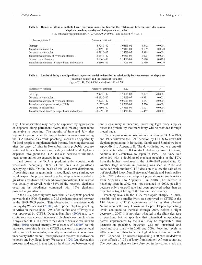
Table 5. Results of fitting a multiple linear regression model to describe the relationship between short-dry seasonelephant poaching density and independent variables

EVI, enhanced vegetation index. F5,86 = 28.820, P< 0.0001 and adjusted R2 = 0.618

Explanatory variable Parameter estimate s.e. t P

Intercept 4.728E–02 1.041E–02 4.542 <0.0001Transformed mean EVI –6.349E–04 1.991E–04 –3.189 0.0020Distance to waterholes 6.711E–07 1.243E–07 5.398 <0.0001Transformed density of rivers and streams 3.564E–02 7.095E–03 5.025 <0.0001Distance to settlements 5.606E–08 2.140E–08 2.620 0.0105Transformed distance to ranger bases and outposts –3.210E–06 1.172E–06 –2.739 0.0076

Table 6. Results of fitting a multiple linear regression model to describe the relationship between wet-season elephant-poaching density and independent variables

F5,86 = 62.140, P < 0.0001 and adjusted R2 = 0.780

Explanatory variable Parameter estimate s.e. t P

Intercept 2.923E–02 3.703E–03 7.893 <0.0001Distance to waterholes –4.293E–07 1.266E–07 –3.391 0.0011Transformed density of rivers and streams 7.372E–02 9.053E–03 8.143 <0.0001Transformed elephant density (2005) 2.177E–02 2.876E–03 7.570 <0.0001Distance to settlements 2.730E–07 2.455E–08 11.121 <0.0001Transformed distance to ranger bases and outposts –8.699E–06 1.345E–06 –6.467 <0.0001

L Wildlife Research J. K. Maingi et al.

consistentwith suggestions byWasser et al. (2010a) that spikes inpoaching are driven more by petitions to down-list and sell ivorythan by the actual sales of ivory.

The positive relationship between poaching density anddensity of elephants suggests that elephant poachers will targetareas with large herds of elephants so as to guarantee maximumreturn for their labour. The positive correlation between densityof poaching and density of rivers and streams may be explainedby elephants’ preference for water and mud baths. As a result,elephants congregate along the rivers and streams, and aroundwaterholes, making them vulnerable to poaching. Ripley’sK function and kernel-density analyses depicted higherconcentrations of poaching along the western edge of theTsavo River, and along both the Galana and Tuva Rivers. Theresults are in agreement with Ottichilo (1987) in that elephantpoaching was concentrated along the central part of GalanaRiver and in the northern and north-western parts of the park.

Studies on social organisation of elephants have shown thatelephants of Tsavo exhibit aggregation all year round (McKnight2000). The aggregations constitute large groups that are notfamily units but those formed in response to stress, harassmentand lack of matriarchs to lead family units as a result of previousheavy poaching (Lewis 1986; Ruggiero 1990). The aggregatingbehaviour of previously heavily poached elephant populationsmay, therefore, explain why elephant mortality exhibitedclustered patterns in the TCA. In addition, poachers often killmore than one large individual elephant in a herd in an effort ofmaximise harvest, thus resulting in clusters of poached-elephantcarcasses.

There was a strong positive correlation between the density ofpoaching and the density of human influences. Poaching alsoincreased as the density of roads increased. Density of poachingwas also positively correlated with the density of roads. Thisfinding is consistent with findings by Barnes et al. (1991) andBlake et al. (2008) in that elephant poaching in theGabon forests,and the Congo Basin, respectively, was concentrated close toroads. These findings suggest that poachers are tolerated or enjoysupport from nearby settlements and towns. The findings alsosuggest that poachers concentrate their activities in areas that arewell served by road networks.

The negative correlation between dry-season poachingdensity and distance to management units was a surprise. Weexpected to find a positive relationship between poachingdensity and distances to management units, indicating thatpoachers confine their activities in remote areas where theywere unlikely to be detected. In the Luangwa Valley, Zambia,Leader-Williams et al. (1990) found that poachers targetedareas with heavy concentrations of elephants, which wereremote and infrequently patrolled by park rangers. Whendistance to ranger bases and outposts in the TCA was teasedout of management units and analysed separately, an evenstronger negative correlation was found between the distanceto ranger bases and outposts, and poaching density across allseasons. This observation suggests that anti-poaching patrolsmay be ineffective or, even more alarming, that there iscollusion between anti-poaching patrol units and poachers. Wehave, however, not come across any reports of KWS personnelcolluding with poachers either from KWS investigators or theever-vigilant and independent Kenyan press. A more plausible

explanation for the negative correlation between elephantpoaching and distance to ranger bases and outpost activitiesis that poaching activities are more likely to be discoveredwhere game rangers are actively patrolling. This would lead todiscoveries of poaching in only the areas within the reach ofpark rangers. Ranger bases and outposts were specifically set upin areas where the KWS management had determined to havehigher incidences of poaching. The implication of our findingsis that it is highly likely that poaching activities go undiscoveredin remote areas of the TCA not reached by anti-poachingpatrols.

Ranger patrol units and ranger-base outposts may not be veryeffective because of insufficient personnel and resources,including vehicles. The work of park rangers and patrols isfurther complicated by inaccessibility of large areas of thepark in the wet season after they are cut off by flooding rivers.It is also quite likely that poachers are not afraid of beingdiscovered and arrested by KWS rangers. When poachers areapprehended by law enforcement with any wildlife trophies,they are taken to court and charged under a law provision(CAP 376 Laws of Kenya) that guarantees a maximum fine ofapproximately $375 or 6 months in jail or both. There have beennumerous reports in the daily newspapers in Kenya whereconvicted poachers were fined $125 in lieu of 3 months in jail.The penalty for poaching is far too lenient, considering that itapplies irrespective of the quantity or type of game trophiesthe poachers are caught with. It is imperative that KWSconduct an assessment of the effectiveness of their rangerbases and outposts in combating poaching. It would beinformative to find out whether poaching incidences aroundthe bases and outposts have been declining or increasing sincetheir establishment.

Elevation was positively correlated with dry-season poachingand negatively correlated with wet-season poaching. Wespeculate that increasing incidences of dry-season poachingwith increasing elevation may be tied to the persistingabundance of browse species favoured by elephants in thoselocations. The negative relationship between elevation and wet-season poaching may indicate that elephants are moving back tothe lower elevations following the rains and greening up of mostvegetation. Poaching density was negatively correlated withmean EVI and the standard deviation of EVI for all seasonsexcept the dry season. Thisfinding is consistentwith other studiesthat found a negative correlation between elephant density andvegetation greenness. Hien et al. (2007), working in the CongoBasin, found that vegetation greenness was negatively correlatedwith elephant density in both the dry andwet seasons. The lack ofa relationship between dry-season EVI and elephant poaching inthe TCAmay be attributed to low greenness in the semiarid TCAin the dry season.

Models to predict overall elephant poaching, and poaching inthe dry, short-dry and wet seasons, all had distance to rangerbases and outposts as an important predictor variable. Threeof the four models had density of rivers and streams, densityof waterholes, distance to settlements and either mean EVI orstandard deviation of EVI as important predictors. With theexception of wet-season poaching, the other poachingprediction models explained less than 70% of the observedvariation in poaching density, indicating that there were

Elephant poaching in Tsavo, Kenya Wildlife Research M

several other important variables linked with elephant poachingthat the present study was unable to identify. This indicatesthe need to identify other predictor variables that have moreexplanatory power. Some of these factors may include measuresthat quantify the attitudes of local communities living in areassurrounding the TCA. Kideghesho et al. (2007) showedprevalence of negative attitudes towards conservation amongcommunities suffering from costs of conservation. These costsmay be tied to government restrictions over access to pastureand water for livestock within conservation areas, or competitionbetween wildlife and livestock for pasture and water withincommunity lands. Other costs to local communities may arisefrom predation of livestock by wildlife and raiding of crops byherbivores. Groom and Harris (2008) showed that the simplepresence of any wildlife benefits to local communities is enoughto positively affect the attitude of local people to wildlife. Otherpredictor variables for poaching should include those measuresthat assess the effectiveness of laws and policies as deterrence topoaching.

Management implications

The present study has demonstrated that elephant-poachinglocations in the TCA are clustered and that these patterns varyby season and by year. The hotspot analysis revealed three mainpoaching hotspots located near the edges of theTCA.The reasonsfor the hotspots in the west and in the north have to do withhuman–wildlife conflicts and the lack of economic opportunitiesfor the local people. Elephants were killed in these locations withpoisoned arrows and spears. It seems that a more concerted effortto solve human–wildlife conflicts in the TWNP–Kajiado Districtboundary would lead to increased cooperation between theKWS and local people and lead to a stemming of elephantpoaching. Elephant poaching along the Tiva River area ofTENP may be linked to a lack of economic opportunities forthe local people. Any efforts made towards improving economicopportunities of the people, would help reduce poaching. Amongthese efforts would be a commitment by the government todevelop infrastructure and tourist facilities in northern Tsavoand aggressively market the area to increase the number oftourists coming to the area. The government should alsoencourage the development of a cottage industry based ontourism, thus giving the local communities a larger stake in theconservation and management of wildlife.

Poaching along the Galana River near the Tana River Districtis a reflection of continuing insecurity in the region, compoundedby infiltration of weapons from neighbouring Somalia whichhas not had a stable government since 1991. Perhaps this is anarea that could benefit from beefing-up of security by both theKWS and the Kenyan Government. It is essential that the lawsregulating poaching in Kenya be made much more punitivebecause, at the present, they do not seem to provide muchdeterrence to poaching. If anything, current laws and policiesmay be demoralising to KWS rangers who after arrestingpoachers and sending them to court see them quickly releasedwith what amounts to a slap on the wrist.

The present study also suggests that there is a need to improvethe reach of KWS patrols and improve the collection of poachingdata by using hand-held GPS rather than approximation of

poaching sites from topographic map. There are vast areas ofthe TCA without a single incident of poaching reported, and itis not clear whether it is because no incidents occurred orwhether it is because KWS did not have the resources toeffectively patrol all the areas. It is time that KWS embarkedon a program to determine the effectiveness of ranger bases andoutposts by examining trends in poaching activities around eachsite since its establishment. Routine use of hand-held GPSreceivers by KWS anti-poaching patrol units would allowKWS managers to determine which areas of the TCA are notbeing patrolled, and thus help clear up some of the uncertaintiesin poaching data collected by the organisation.

AcknowledgementsWe are most grateful to the Kenya Wildlife Service for availing elephantpoaching data and for providing some of theGIS data.We aremost grateful toDr Mary Henry and Dr Jerry Green for reviewing earlier versions of thismanuscript.We also thankDr JonPatton for advicewith someof the statisticalanalyses. We thank the three anonymous reviewers for the very many usefulcomments andsuggestions theyprovided.Webelieve their efforts havehelpedimprove the quality of our manuscript. Any opinions expressed in this paperare those of the authors and do not constitute policy of the Kenya WildlifeService.

References

Anselin, L., Cohen, J., Cook, D., Gorr, W., and Tita, G. (2000). Spatialanalyses of crime. Criminal Justice 4, 213–262.

Bailey, T. C., and Gatrell, A. C. (1995). ‘Interactive Spatial Data Analysis.’(Longman Scientific and Technical: Harlow, Essex, UK.)

Barnes, J. I. (1996). Changes in the economic use value of elephant inBotswana: the effect of international trade prohibition. EcologicalEconomics 18(3), 215–230. doi:10.1016/0921-8009(96)00035-3

Barnes, R. F. W., Barnes, K. L., Alers, M. P. T., and Blom, A. (1991). Mandetermines the distribution of elephants in the rain forests of northeasternGabon. African Journal of Ecology 29(1), 54–63. doi:10.1111/j.1365-2028.1991.tb00820.x

Blake, S., Deem, S. L., Strindberg, S., Maisels, F., Momont, L., Isia, I. B.,Douglas-Hamilton, I., Karesh, W. B., and Kock, M. D. (2008).Roadless wilderness area determines forest elephant movements in theCongo Basin. PLoS ONE 3(10), e3546. doi:10.1371/journal.pone.0003546

Boslaugh, S., and Watters, P. A. (2008). ‘Statistics in a Nutshell: a DesktopQuick Reference.’ (O’Reilly Media Inc.: Sebastopol, CA.)

Bulte, E. H., Damania, R., andKooten, G. C. V. (2007). The effects of one-offivory sales on eephant mortality. The Journal of Wildlife Management 71(2), 613–618. doi:10.2193/2005-721

Burnham, K. P., Anderson, D. R., and Burnham, K. P. (2002). ‘ModelSelection and Multimodel Inference: a Practical Information-theoreticApproach.’ (Springer: New York.)

Burton, M. (1999). An assessment of alternative methods of estimating theeffect of the ivory trade ban on poaching effort. Ecological Economics 30(1), 93–106. doi:10.1016/S0921-8009(98)00102-5

Chamaillé-Jammes, S., Valeix, M., and Fritz, H. (2007). Managingheterogeneity in elephant distribution: interactions between elephantpopulation density and surface-water availability. Journal of AppliedEcology 44(3), 625–633. doi:10.1111/j.1365-2664.2007.01300.x

CITES (2009). How CITES works. In ‘Convention on InternationalTrade in Endangered Species of Wild Fauna and Flora’. Availableat http://www.cites.org/eng/disc/how.shtml [Verified 16 October2010]

N Wildlife Research J. K. Maingi et al.

Cohen, L. E., and Felson,M. (1979). Social cange and crime trends: a routineactivity approach. American Sociological Review 44, 588–608.doi:10.2307/2094589

Cohn, J. P. (1990). Elephants: remarkable and endangered. Bioscience 40(1),10–14. doi:10.2307/1311233

Douglas-Hamilton, I. (1987). African elephant population study. Pachyderm8, 1–10.

Douglas-Hamilton, I. (2009). The current elephant poaching trend.Pachyderm 45, 154–157.

ESRI (2011). ‘ArcGISDesktop.’ (Environmental SystemsResearch Institute:Redlands, CA.)

Gao, X., Huete, A. R., Ni, W., and Miura, T. (2000). Optical–biophysicalrelationships of vegetation spectra without background contamination.Remote Sensing of Environment 74(3), 609–620. doi:10.1016/S0034-4257(00)00150-4

Gatrell, A. C., Bailey, T. C., Diggle, P. J., and Rowlingson, B. S. (1996).Spatial point pattern analysis and its application in geographicalepidemiology. Transactions of the Institute of British Geographers 21,256–274. doi:10.2307/622936

Gillson, L. (2004). Testing non-equilibrium theories in savannas: 1400 yearsof vegetation change in Tsavo National Park, Kenya. EcologicalComplexity 1(4), 281–298. doi:10.1016/j.ecocom.2004.06.001

Greenway, P. (1969). A check-list of plants recorded in Tsavo National Park.Journal of East Africa Natural History Society and National Museum 27,161–209.

Griffith, D. A. (1985). An evaluation of correction techniques for boundaryeffects in spatial statistical analysis: contemporary methods.Geographical Analysis 17(1), 81–88. doi:10.1111/j.1538-4632.1985.tb00828.x

Groom, R., and Harris, S. (2008). Conservation on community lands: theimportance of equitable revenue sharing.Environmental Conservation 35(3), 242–251. doi:10.1017/S037689290800489X

Hien, B. M., Jenks, J. A., Klaver, R. W., and Wicks, Z. W. (2007).Determinants of elephant distribution at Nazinga Game Ranch,Burkina Faso. Pachyderm 42(January–June), 70–80.

Hosmer,D.W., Jovanovic,B., andLemeshow,S. (1989).Best subsets logisticregression. Biometrics 45(4), 1265–1270. doi:10.2307/2531779

Jachmann, H., and Billiouw, M. (1997). Elephant poaching and lawenforcement in the central Luangwa Valley, Zambia. Journal ofApplied Ecology 34(1), 233–244. doi:10.2307/2404861

Jiang, Z., Huete, A. R., Didan, K., and Miura, T. (2008). Development ofa two-band enhanced vegetation index without a blue band. RemoteSensing of Environment 112(10), 3833–3845. doi:10.1016/j.rse.2008.06.006

Kaltenbach, H.-M. (2012). ‘A Concise Guide to Statistics.’ (Springer: NewYork.)

Kideghesho, J., Røskaft, E., and Kaltenborn, B. (2007). Factors influencingconservation attitudes of local people in western Serengeti, Tanzania.Biodiversity and Conservation 16(7), 2213–2230. doi:10.1007/s10531-006-9132-8

Leader-Williams,N. (1994).Thecost of conservingelephants.Pachyderm18,30–34.

Leader-Williams, N., Albon, S. D., and Berry, P. S. M. (1990). Illegalexploitation of black rhinoceros and elephant populations: patternsof decline, law enforcement and patrol effort in Luangwa Valley,Zambia. Journal of Applied Ecology 27(3), 1055–1087. doi:10.2307/2404395

Lemieux,A.M., andClarke,R.V. (2009).The international banon ivory salesand its effects on elephant poaching in Africa. The British Journal ofCriminology 49(4), 451–471. doi:10.1093/bjc/azp030

Leuthold,W. (1977). Spatial organization and strategy of habitat utilization ofelephants in Tsavo National Park, Kenya. Mammalian Biology -Zeitschrift fur Saugetierkunde 42, 358–379.

Lewis, D. M. (1986). Disturbance effects on elephant feeding: evidence forcompression in LuangwaValley, Zambia.African Journal of Ecology 24,227–241. doi:10.1111/j.1365-2028.1986.tb00367.x

Loarie, S. R., van Aarde, R. J., and Pimm, S. L. (2009). Elephant seasonalvegetation preferences across dry and wet savannas. BiologicalConservation 142(12), 3099–3107. doi:10.1016/j.biocon.2009.08.021

McKnight, B. (2000). Changes in elephant demography, reproduction andgroup structure in TsavoEast National Park (1966–1994).Pachyderm 29,15–24.

Messer, K. (2000). The poacher’s dilemma: the economics of poaching andenforcement. Endangered Species UPDATE 17(3), 50–56.

METI NASA (2009). ‘Aster Global Digital Elevation Model. Version 1,2009.’ (Ministry of Economy, Trade and Industry (METI): Japan; andNASA). Available at https://wist.echo.nasa.gov/~wist/api/imswelcome/[Verified 3 October 2010]

Milner-Gulland, E. J., and Leader-Williams, N. (1992). Amodel of incentivesfor the illegal exploitationofblack rhinos andelephants–Poachingpays inLuangwa Valley, Zambia. Journal of Applied Ecology 29(2), 388–401.doi:10.2307/2404508

Moran, P. A. P. (1950). Notes on continuous phenomena. Biometrica 37,17–33.

Mukeka, J. M. (2010). ‘Analyzing the Distribution of the African Elephant(Loxodontaafricana) inTsavo,Kenya.’ (MiamiUniversity:Oxford,OH.)

O’Sullivan, D., andUnwin, D. J. (2003). ‘Geographic InformationAnalysis.’(John Wiley & Sons: Hoboken, NJ.)

Ottichilo, W. K. (1987). The causes of the recent heavy elephant mortality intheTsavo ecosystem,Kenya, 1975–1980.Biological Conservation 41(4),279–289. doi:10.1016/0006-3207(87)90091-7

Redfern, J. V., Grant, R., Biggs, H., and Getz, W. M. (2003). Surface-waterconstraints on herbivore foraging in the Kruger National Park, SouthAfrica. Ecology 84, 2092–2107. doi:10.1890/01-0625

Ripley, B. D. (1976). The second-order analysis of stationary pointprocesses. Journal of Applied Probability 13, 255–266. doi:10.2307/3212829

Ruggiero, R. (1990). The effects of poaching disturbance on elephantbehaviour. In ‘Pachyderm – Newsletter of the African Elephant &Rhino Specialist Group. Number 13’. (Eds C. G. Gakahu, B. Goode,D.Western,E.B.MartinandL.Vigne)pp.44–46. (InternationalUnion forConservation of Nature & Wildlife Conservation International: Nairobi:Kenya)

Santiapillai, C. (2009). African elephants: surviving by the skin of their teeth.Current Science 97(7), 996–997.

Simons, R. T., and Kreuter, U. P. (1989). Herd mentality: banning ivory salesis no way to save the elephant. Policy Review 50, 46–49.

Sokal, R. R., and Oden, N. L. (1978). Spatial autocorrelation in biology 1.Methodology. Biological Journal of the Linnean Society. LinneanSociety of London 10(2), 199–228. doi:10.1111/j.1095-8312.1978.tb00013.x

Stiles, D. (2004). The ivory trade and elephant conservation. EnvironmentalConservation 31(4), 309–321. doi:10.1017/S0376892904001614

Van Dijk, J. J. M. (1994). Understanding crime rates: on the interactionbetween rational choices of victims and offenders. The British Journal ofCriminology 34(2), 105–121.

Verlinden, A., and Gavor, I. K. N. (1998). Satellite tracking of elephants innorthern Botswana. African Journal of Ecology 36(2), 105–116.

Walker, J. F., and Stiles, D. (2010). Consequences of Legal IvoryTrade. Science 328(5986), 1633–1634. doi:10.1126/science.328.5986.1633-c

Wasser, S. K., Mailand, C., Booth, R., Mutayoba, B., Kisamo, E., Clark, B.,and Stephens, M. (2007). Using DNA to track the origin of the largestivory seizure since the 1989 trade ban. Proceedings of the NationalAcademy of Sciences, USA 104(10), 4228–4233. doi:10.1073/pnas.0609714104

Elephant poaching in Tsavo, Kenya Wildlife Research O

Wasser, S., Nowak, K., Poole, J., Hart, J., Beyers, R., Lee, P., Lindsay, K.,Brown,G., Granli, P., andDobson,A. (2010a). Response – consequencesof legal ivory trade. Science 328(5986), 1634–1635. doi:10.1126/science.328.5986.1634-d

Wasser, S., Poole, J., Lee, P., Lindsay, K., Dobson, A., Hart, J., Douglas-Hamilton, I., Wittemyer, G., Granli, P., Morgan, B., Gunn, J., Alberts,S., Beyers, R., Chiyo, P., Croze, H., Estes, R., Gobush, K., Joram, P.,Kikoti, A., Kingdon, J., King, L., Macdonald, D., Moss, C., Mutayoba,B., Njumbi, S., Omondi, P., and Nowak, K. (2010b). Elephants, ivory,and trade. Science 327(5971), 1331–1332. doi:10.1126/science.1187811

Western, D. (1975). Water availability and its influence on the structure anddynamics of savannah large mammal community. East African WildlifeJournal 13, 265–286.

Wong, D. W. S., and Lee, J. (2005). ‘Statistical Analysis of GeographicInformation with ArcViewGIS and ArcGIS.’ (JohnWiley and Sons Inc.:Hoboken, NJ.)

P Wildlife Research J. K. Maingi et al.

www.publish.csiro.au/journals/wr