Environ Monit Assess (2011) 173:625–641DOI 10.1007/s10661-010-1411-x

Spatial water quality assessment of Langat River Basin(Malaysia) using environmetric techniques

Hafizan Juahir · Sharifuddin M. Zain · Mohd Kamil Yusoff ·T. I. Tengku Hanidza · A. S. Mohd Armi ·Mohd Ekhwan Toriman · Mazlin Mokhtar

Received: 13 December 2008 / Accepted: 24 February 2010 / Published online: 27 March 2010© The Author(s) 2010. This article is published with open access at Springerlink.com

Abstract This study investigates the spatial waterquality pattern of seven stations located alongthe main Langat River. Environmetric methods,namely, the hierarchical agglomerative clusteranalysis (HACA), the discriminant analysis (DA),the principal component analysis (PCA), and thefactor analysis (FA), were used to study the spatialvariations of the most significant water qualityvariables and to determine the origin of pollution

H. Juahir (B) · M. K. Yusoff ·T. I. T. Hanidza · A. S. M. ArmiDepartment of Environmental Science,Faculty of Environmental Studies,Universiti Putra Malaysia,43400 Serdang, Selangor, Malaysiae-mail: hafizan@env.upm.edu.my

A. S. M. Armie-mail: armyfor@yahoo.com

S. M. ZainDepartment of Chemistry, Faculty of Science,University of Malaya,56000 Kuala Lumpur, Malaysia

M. E. TorimanSchool of Social Development and EnvironmentalStudies, Universiti Kebangsaan Malaysia,43600 Bangi, Selangor, Malaysia

M. MokhtarInstitute of Environment and Development(LESTARI), Universiti Kebangsaan Malaysia,43600 Bangi, Selangor, Malaysia

sources. Twenty-three water quality parameterswere initially selected and analyzed. Three spatialclusters were formed based on HACA. Theseclusters are designated as downstream of Langatriver, middle stream of Langat river, and upstreamof Langat River regions. Forward and backwardstepwise DA managed to discriminate six andseven water quality variables, respectively, fromthe original 23 variables. PCA and FA (varimaxfunctionality) were used to investigate the originof each water quality variable due to land use ac-tivities based on the three clustered regions. Sevenprincipal components (PCs) were obtained with81% total variation for the high-pollution source(HPS) region, while six PCs with 71% and 79%total variances were obtained for the moderate-pollution source (MPS) and low-pollution source(LPS) regions, respectively. The pollution sourcesfor the HPS and MPS are of anthropogenicsources (industrial, municipal waste, and agricul-tural runoff). For the LPS region, the domes-tic and agricultural runoffs are the main sourcesof pollution. From this study, we can concludethat the application of environmetric methods canreveal meaningful information on the spatial vari-ability of a large and complex river water qualitydata.

Keywords Environmetric · Water quality ·Cluster analysis · Discriminant analysis ·Principal component analysis · Factor analysis

626 Environ Monit Assess (2011) 173:625–641

Introduction

The State of Selangor, Malaysia, has a long historyof river pollution problems associated with landuse changes. The Langat River is one of the prin-cipal river draining a densely populated and de-veloped area of Selangor. Over the past 40 years,it has served about half of the population ofSelangor and is a source of hydropower and con-trol of flood discharges. More than two third of theSelangor population inhabit the floodplain, whichprovides highly fertile land for agriculture andland for housing, recreation, and industrial devel-opments. This scenario has brought humans intoconflict of harmony between human developmentand river environment and increases the degree ofpollution into river channels. According to Aikenet al. (1982), 42 tributaries in Peninsular Malaysiahave been categorized as very polluted, includingthe Langat River. Until 1999, there were 13 pol-luted tributaries all over Malaysia with 36 pollutedrivers due to human activities such as industry,construction, and agriculture at the tributaries(Department of Environment 1999). In 1990,there were 48 clean rivers compared to only 32rivers in 1999 that could still be classified as clean(Rosnani 2001).

Almost 60% of the major rivers are regulatedfor domestic, agricultural, and industrial purposes(Department of Irrigation and Drainage 2001).According to Rosnani (2001), the major pollutionsources affecting rivers in Malaysia are sewagedisposal, discharges from small- and medium-sized industries that are still not equipped withproper effluent treatment facilities and land clear-ing and earthworks activities. In 1999, 42% ofthe river basins were recorded to be pollutedwith suspended solids (SS) resulting from poorlyplanned and uncontrolled land clearing activities,30% with biological oxygen demand (BOD) fromindustrial discharges, and 28% with ammoniacalnitrogen (AN) from animal husbandry activitiesand domestic sewage disposal.

Surface water pollution is identified as the ma-jor problem affecting the Langat River Basin inMalaysia. The increase of developing areas withinthe river basin increases pollution loading into theLangat River. As an effort to avoid the LangatRiver from becoming more polluted, the Depart-

ment of Environment (DOE) of Malaysia, Min-istry of Natural Resources and Environment ofMalaysia, has installed telemetric stations alongthe river basin to continuously monitor its waterquality. Based on the water quality data, the waterquality index (WQI) was developed to evaluatethe water quality status and river classification.WQI provides a useful way to predict changes andtrends in the water quality by considering multipleparameters. WQI is formed by six selected waterquality variables, namely, dissolved oxygen (DO),BOD, chemical oxygen demand (COD), SS, AN,and pH (DOE 1997).

Rapid urbanization along the Langat Riverplays an important role in the increase of pointsource (PS) and non-point source (NPS) pollutionloading. The water quality in the basin has beendeteriorating over the years, as evidenced fromthe water quality database compiled for 15 years.The recorded WQI ranged from 58.1 to 75, whichcorresponds to polluted (WQI, 0–59) and moder-ately polluted (WQI, 60–80). Based on the aver-age values taken from the 2002 survey (Table 1and Fig. 1), the major pollutants in the LangatRiver Basin expressed as percentage of stationsexhibiting quality corresponding to class 3 andabove are as follows (figures in parenthesis indi-cate percent sampling stations): AN (94%), TSSand BOD (71%), COD (65%), and DO (53%;UPUM 2002).

From this survey, the NPS pollution is seen asthe main contributor to the pollution load com-pared to PS pollution (UPUM 2002). Due to theexponential increase in urbanization within theLangat River Basin, a review of WQI, is required.In this light, spatial temporal evaluation of riverwater quality variations along the Langat River isinitiated.

Spatial analysis is conducted to evaluate themost significant water quality parameters, takinginto account land use activities that affect thehealth of the river. The transformation of a par-ticular type of land use, such as agriculture andforest area into industrial or municipal area, willchange the types of pollutant loadings into theriver system. Since there are numerous PS andNPS pollution sources along the Langat River, it isquite a challenge to identify the origin of each pol-lutant. Regular monitoring by DOE provides the

Environ Monit Assess (2011) 173:625–641 627

Table 1 Comparisonbetween total pointsource and non-pointsource pollution loadcontribution in theLangat River Basin basedon the event samplingapproach

UPUM (2002)

Pollution source Pollution loading (t/day)

COD BOD TSS TM AN

Industry 22.650 5.536 14.414 0.2440 1.513Wet market 1.070 0.384 0.409 0.0050 0.056Pig farm 1.020 0.201 0.460 0.0056 0.725Public sewage treatment plants 20.680 5.047 5.692 0.0890 3.071Private sewage treatment plants 4.340 1.060 1.200 0.0200 0.640Individual sewage treatment plants 17.260 7.140 8.354 0.0000 2.784Landfill 5.650 1.048 8.149 0.0310 0.664Sand mining 20.880 0.820 206.670 2.7780 0.057Total PS 93.550 21.240 245.350 3.1700 9.510Total NPS (t/day) 614.950 132.690 2,791.030 15.2500 12.670% PS 13.2 13.8 8 17.2 42.8% NPS 86.8 86.2 92 82.8 57.2

available spatial variation data. However, inter-preting the huge amount of data is a challengerequiring one to use correct methods of data in-terpretation (Chapman 1992; Dixon and Chiswell1996).

Environmetrics can be considered as a branchof environmental analytical chemistry that usesmultivariate statistical modeling and data treat-ment also known as chemometrics; (Simeonovet al. 2000). Environmetric is deemed to bethe best approach to avoid misinterpretation ofa large complex environmental monitoring data(Simeonov et al. 2002). Environmetric methodshave been widely used in drawing meaning-ful information from masses of environmentaldata. These methods have often been used inexploratory data analysis tools for classification(Brodnjak-Voncina et al. 2002; Kowalkowski et al.

2006) of samples (observations) or sampling sta-tions and the identification of pollution sources(Massart et al. 1997; Vega et al. 1998; Shrestha andKazama 2007). Environmetrics have also beenapplied to characterize and evaluate the surfaceand freshwater quality as well as verifying spatialvariations caused by natural and anthropogenicfactors (Helena et al. 2000; Singh et al. 2005;Juahir et al. 2008). Recently, environmetric meth-ods have become an important tool in environ-mental sciences (Brown et al. 1994, 1996) to revealand evaluate complex relationships in a wide vari-ety of environmental applications (Alberto et al.2001). The most common environmetric methodsused for clustering are the hierarchical agglomera-tive cluster analysis (HACA) and the principalcomponents analysis (PCA) with factor analysis(FA; Kannel et al. 2007). These methods are

Fig. 1 Percentagecontribution of each typeof point source ofpollution in the LangatRiver Basin

2.35

84.09

0.36

4.16

0.90

5.97

1.81

0.36

0.00 10.00 20.00 30.00 40.00 50.00 60.00 70.00 80.00 90.00

Wet Market

Factory

Pig Farm

Sand Mine

Landfill

Public STP

Private STP

Workshop

Percentage of Point Sources Pollution

Source: UPUM (2002)

628 Environ Monit Assess (2011) 173:625–641

commonly supported by discriminant analysis(DA) as a confirmation for HACA and PCA andare usually referred to as pattern recognitionmethods (Adams 1998). The application of dif-ferent pattern recognition techniques to reduce thecomplexity of large data sets has proven to give abetter interpretation and understanding of waterquality data (Brown et al. 1980; Qadir et al. 2007).

The objective of this study is to evaluate thespatial variations in the river water quality datamatrix taken from the Langat River (PeninsularMalaysia) using environmetric methods. The dataare taken from the river quality monitoring pro-gram of 1995–2002. Environmetric methods wereused to identify the influence of land use activitieson the spatial variations of Langat River waterquality. Based on the information obtained fromthis study, a critique on the WQI methodology willbe presented.

Methodology

Description of study area

The Langat River has a total catchment area ofapproximately 1,815 km2. It lies within latitudes2◦40′ M 152′′ N to 3◦16′ M 15′′ and longitudes101◦19′ M 20′′ E to 102◦1′ M 10′′ E. The catch-ment is illustrated in Fig. 2. The Langat RiverBasin formed by 15 sub-basins, namely, Pangsoon,Hulu Lui, Hulu Langat, Cheras, Kajang, Putra-jaya, Hulu Semenyih, Semenyih, Batang Benar,Batang Labu, Beranang, Bangi Lama, Rinching,Teluk Datok, and Teluk Panglima Garang. Themain river course length is about 141 km, mostlysituated around 40 km east of Kuala Lumpur.The Langat River has several tributaries withthe principal ones being the Semenyih River,the Lui River, and the Beranang River. There

Legend Rainfall station

2815001

2818110

2913001

2917001

3018101

3118102

3119104

Main river

Sub-basin

"

2815001

2818110

2913001

2917001

2916001

3018101

3118102

3119104

Discharge station

2816441

2917641

Fig. 2 Seven water quality stations (Sb) were selected in this study along the main river

Environ Monit Assess (2011) 173:625–641 629

are two reservoirs, the Langat Reservoir and theSemenyih Reservoir catchments, respectively. TheLangat Reservoir, built in 1981, has a catchmentarea of 54 km2, while the Semenyih Reservoir,built in 1982 with the purpose to supply domes-tic and industrial water, has a catchment area of41 km2. For the Langat Reservoir, it is also usedto generate power supply at moderate capacity forthe population within the Langat Valley.

This climate in the study area is characterizedby high average and uniform annual tempera-tures, high rainfall, and high humidity. This cli-mate has a dominant impact on the hydrology andgeomorphology of the study area. Generally, thestudy area experiences two types of season: thewet season in April to November and a relativelydrier period from January to March. The weatheris very much influenced by the SW monsoon thatblows across the Straits of Malacca. Flooding iscommon in the study area.

The study areas include selected impactedand non-impacted stretches of the Sungai LangatBasin. Starting from the Semenyih and HuluLangat Dams, down to the lowest area at theestuary near Permatang Pasir, with a total distanceof 78 km. Due to immense area (1,987.7 km2), it iscrucial that critically impacted areas be identified.

The data and monitoring sites

The water quality data in this study were ob-tained from seven stations along the main LangatRiver (Fig. 2). The water quality monitoring sta-tions are manned by the Department of Environ-

ment (DOE), Ministry of Natural Resource andEnvironment of Malaysia. The selected stationsare illustrated in Table 2. All the stations wereidentified based on the availability of recordeddata from 1995 to 2002. The data collected fromSeptember 1995 to May 2002 were selected forthis study. Referring to the sampling sites mannedby DOE in the present study, a total of sevensites represent the eight Langat sub-basin, namely,Teluk Panglima Garang (site 7), Teluk Datok(site 6), Putrajaya (site 5), Kajang (site 4), Cheras(site 3), Hulu Langat (site 2), Pangsoon, and UluLui (site 1). Sites 3–7 are located in the region ofhigh pollution load, as there are several wastewa-ter drains situated in the middle and downstreamof the Langat River Basin. Site 2 is partly situatedin the middle stream region of moderate riverpollution. Site 1 and a part of site 2 are locatedupstream of the Langat River, in the area of rel-atively low river pollution. It is worth mentioningthat some stations have missing data and not allstations were consistently sampled.

Although there are 30 water quality parame-ters available, only 23 consistently sampled pa-rameters were selected. A total of 254 sampleswere used for the analysis. The 23 water qualityparameters are DO, BOD, electrical conductivity(EC), COD, AN, pH, SS, temperature (T), salinity(Sal), turbidity (Tur), dissolved solid (DS), totalsolid (TS), nitrate (NO−

3 ), chlorine (Cl), phos-phate (PO−

4 ), zinc (Zn), calcium (Ca), iron (Fe),potassium (K), magnesium (Mg), sodium (Na),Escherichia coli, and coliform. The descriptive sta-tistics of the measured 8-year data set are summa-rized in Table 3.

Table 2 DOE samplingstation at the study area

DOE Study Distance from Grid reference Locationstation no. code estuary (km)

2814602 Sb07 4.19 2◦52.027′ 101◦26.241′ Air Tawar Village2815603 Sb06 33.49 2◦48.952′ 101◦30.780′ Telok Datuk,

near Banting town2817641 Sb05 63.43 2◦51.311′ 101◦40.882′ Bridge at Dengkil Village2918606 Sb04 81.14 2◦57.835′ 101◦47.030′ Near West Country Estate2917642 Sb03 86.94 2◦59.533′ 101◦47.219′ Kajang Bridge3017612 Sb02 93.38 2◦02.459′ 101◦46.387′ Junction to Serdang,

Cheras at Batu 113118647 Sb01 113.99 3◦09.953′ 101◦50.926′ Bridge at Batu 18

630 Environ Monit Assess (2011) 173:625–641

Tab

le3

Mea

nva

lues

ofw

ater

qual

ity

mea

sure

men

talo

ngth

eL

anga

tRiv

erdu

ring

1995

–200

2

Var

iabl

eSt

atio

n1

(Sb0

1)St

atio

n2

(Sb0

2)St

atio

n3

(Sb0

3)St

atio

n4

(Sb0

4)St

atio

n5

(Sb0

5)St

atio

n6

(Sb0

6)St

atio

n7

(Sb0

7)

Mea

nSD

Mea

nSD

Mea

nSD

Mea

nSD

Mea

nSD

Mea

nSD

Mea

nSD

DO

2.54

1.63

3.85

1.52

3.85

1.52

3.71

1.95

3.03

0.29

6.01

1.19

7.54

0.52

BO

D8.

1313

.72

6.28

3.94

6.28

3.94

15.3

715

.03

13.3

11.

748.

5110

.51

2.36

1.98

CO

D21

9.27

678.

944

.97

29.2

444

.97

29.2

460

.64

33.7

560

.57

5.76

43.4

739

.42

14.3

12.8

2SS

357.

3959

4.33

564.

3160

3.1

564.

3160

3.1

528.

9288

5.68

417.

111

5.98

468.

560

9.28

27.7

667

.84

pH6.

440.

96.

450.

326.

450.

326.

390.

596.

620.

066.

60.

237.

090.

37A

N0.

831.

071.

792.

441.

792.

442.

021.

52.

130.

191.

681.

330.

120.

14T

emp.

30.7

11.

5729

.06

1.55

29.0

61.

5529

.01

1.99

28.7

80.

2828

.41

2.02

28.2

61.

86E

C20

,128

.33

12,2

75.4

411

5.91

54.4

511

5.91

54.4

512

7.87

77.7

515

8.43

15.0

282

.444

.75

32.7

87.

05Sa

l14

.14

7.85

0.06

0.09

0.06

0.09

0.03

0.04

0.05

0.01

0.01

00.

010.

02T

ur.

516.

376

5.09

721.

677

3.76

721.

677

3.76

506.

6150

2.58

346.

6765

.59

756.

931,

402.

8813

.97

20.9

DS

15,3

11.1

98,

255.

7168

.01

31.6

568

.01

31.6

577

.16

36.7

587

.93

6.77

58.7

229

.75

30.7

21.0

3T

S15

,668

.59

8,12

3.29

632.

3259

6.63

632.

3259

6.63

606.

0787

7.67

505.

0311

3.46

527.

2260

4.9

58.7

67.6

4N

O− 3

0.99

1.55

1.78

2.32

1.78

2.32

0.81

0.92

1.01

0.24

1.66

2.23

0.81

0.74

Cl

8,19

7.19

4,29

4.78

7.33

5.12

7.33

5.12

7.11

4.78

10.8

41.

454.

893.

261.

220.

38P

O− 4

0.07

0.14

0.11

0.18

0.11

0.18

0.11

0.17

0.16

0.07

0.12

0.18

0.09

0.16

Zn

0.05

0.07

0.06

0.1

0.06

0.1

0.04

0.05

0.04

0.01

0.04

0.06

0.04

0.05

Ca

156.

9184

.96

8.54

2.92

8.54

2.92

9.07

3.63

11.6

80.

746.

623.

482.

291.

01F

e0.

480.

871.

972.

161.

972.

161.

923.

11.

980.

811.

922.

540.

340.

24K

169.

6410

0.53

4.54

1.38

4.54

1.38

4.44

1.36

4.69

0.29

3.46

1.03

2.24

0.47

Mg

477.

5329

3.36

1.16

0.51

1.16

0.51

0.93

0.38

1.22

0.09

0.72

0.38

0.59

0.28

Na

4,24

0.21

2,42

4.17

7.79

5.23

7.79

5.23

8.53

4.02

10.2

21.

186.

042.

92.

821.

07E

.col

i1,

518.

554,

473.

3731

,943

.61

48,0

68.5

531

,943

.61

48,0

68.5

587

,789

.72

77,4

39.7

583

,715

.24

12,0

69.4

954

,866

53,5

93.1

512

,477

.67

34,2

89.8

9C

olif

orm

24,6

39.3

310

4,14

4.69

92,6

2110

4,66

9.35

92,6

2110

4,66

9.35

192,

275

245,

384.

1116

4,45

039

,805

.99

959,

673.

334,

353,

732.

510

9,65

9.7

289,

274.

59

Environ Monit Assess (2011) 173:625–641 631

Cluster analysis

In this study, HACA was employed to inves-tigate the grouping of the sampling sites (spa-tial). HACA is a common method to classify(Massart and Kaufman 1983) variables or cases(observations/samples) into clusters with high ho-mogeneity level within the class and high het-erogeneity level between classes with respect toa predetermined selection criterion (McKenna2003). Ward’s method using euclidean distancesas a measure of similarity (Willet 1987; Adams1998; Otto 1998) within HACA has proved to bea very efficient method. The result is illustratedby a dendogram, presenting the clusters and theirproximity (Forina et al. 2002). The euclidean dis-tance (linkage distance) is reported as Dlink/Dmax,which represents the quotient between the linkagedistance divided by the maximal distance. Thequotient is usually multiplied by 100 as a way tostandardize the linkage distance represented bythe y-axis (Singh et al. 2004, 2005; Shrestha andKazama 2007).

Discriminant analysis

Discriminant analysis determines the variablesthat discriminate between two or more naturallyoccurring groups/clusters. It constructs a discrim-inant function (DF) for each group (Johnson andWichern 1992). DFs are calculated using Eq. 1:

f (Gi) = ki +n∑

j=1

wij Pij (1)

where i is the number of groups (G), ki is theconstant inherent to each group, n is the numberof parameters used to classify a set of data intoa given group, and wj is the weight coefficientassigned by DF analysis (DFA) to a given para-meter (pj).

In this study, DA was applied to determinewhether the groups differ with regard to the meanof a variable and to use that variable to pre-dict group membership. Three groups for spatialanalysis (three sampling regions represents up-stream, middle stream, and downstream), whichwere determined from CA, were selected. TheDA was applied to the raw data using the stan-

dard, forward stepwise, and backward stepwisemodes. These were used to construct DFs to eval-uate spatial variations in the river water quality.The stations (spatial) were the grouping (depen-dent) variables, while all the measured parametersconstitute the independent variables. In the for-ward stepwise mode, variables are included stepby step beginning with the most significant vari-able until no significant changes were obtained.In the backward stepwise mode, variables are re-moved step by step beginning with the less sig-nificant variable until no significant changes wereobtained.

Principal component analysis/factor analysis

The most powerful pattern recognition techniquethat is usually coupled with HACA is the PCA.It provides information on the most significantparameters due to spatial and temporal variationsthat describes the whole data set by excludingthe less significant parameters with minimum lossof original information (Singh et al. 2004, 2005;Kannel et al. 2007). The principle component(PC) can be expressed as

zij = ai1x1 j + ai2x2 j + ... + aimxmj (2)

where z is the component score, a is the compo-nent loading, x is the measured value of the vari-able, i is the component number, j is the samplenumber, and m is the total number of variables.

The FA is usually applied as a method to in-terpret a large complex data matrix and offers apowerful means of detecting similarities amongvariables or samples (Reghunath et al. 2002). ThePCs generated by PCA are sometimes not readilyinterpreted; therefore, it is advisable to rotatethe PCs by varimax rotation. Varimax rotationsapplied on the PCs with eigenvalues more than 1are considered significant (Kim and Mueller1987) in order to obtain new groups of variablescalled varimax factors (VFs). The number of VFsobtained by varimax rotations is equal to the num-ber of variables in accordance with common fea-tures and can include unobservable, hypothetical,and latent variables (Vega et al. 1998). The VFcoefficients having a correlation greater than 0.75

632 Environ Monit Assess (2011) 173:625–641

are considered as “strong”; 0.75–0.50, as “moder-ate”; and 0.50–0.30, as “weak” significant factorloadings (Liu et al. 2003).

Source identification of different pollutants wasmade on the basis of different activities in thecatchment area in light of previous literatures. Thebasic concept of FA is expressed as

zij = a f 1 f1i + a f 2 f21 + .... + a f m fmi + e f i (3)

where z is the measured value of a variable, ais the factor loading, f is the factor score, e isthe residual term accounting for errors or othersources of variation, i is the sample number, j isthe variable number, and m is the total number offactors.

In this study, PCA/FA was applied to the nor-malized data sets (23 variables) separately for thethree different spatial regions, HPS, MPS, andLPS, as delineated by the CA technique. The in-put data matrices (variables × cases) for PCA/FAwere 23 × 69 for HPS, 23 × 120 for MPS, and23 × 65 for LPS regions.

Results and discussion

Classification of sampling station based onhistorical water quality data

This section examines the historical values of wa-ter quality parameters in order to classify thewater quality station based on their similarity levelusing HACA. HACA was performed on the wa-ter quality data set to evaluate spatial variationamong the sampling sites. This analysis resulted

in the grouping of sampling stations into threeclusters/groups (Fig. 3).

Cluster 1 (stations Sb01 and Sb02) representsthe low-pollution source (LPS) from the sub-basin Pangsoon and Ulu Lui, cluster 2 (stationsSb03, Sb04, and Sb05) represents the moderate-pollution sources (MPS) from Cheras and HuluLangat, and cluster 3 (stations Sb06 and Sb07)represents the high-pollution sources (HPS) fromsub-basin Kajang, Putrajaya, Teluk Datok, andTeluk Panglima Garang.

This result implies that for rapid assessment ofwater quality, only one station in each cluster isneeded to represent a reasonably accurate spatialassessment of the water quality for the wholenetwork. The CA technique reduces the needfor numerous sampling stations. Monitoring from3 stations that represent three different regionsis sufficient. It is evident that the HACA tech-nique is useful in offering reliable classificationof surface water for the whole region and can beused to design future spatial sampling strategiesin an optimal manner. Figure 4 shows the threeregions given by HACA and the possible pollu-tion sources within the study regions. The clus-tering procedure generated three groups/clustersin a very convincing way, as the sites in thesegroups have similar characteristics and naturalbackgrounds.

Spatial variations of river water quality

To study the spatial variation among the differentstream regions, DA was applied on the raw datapost grouping of the Langat Basin into three mainclusters/groups defined by CA. Groups (HPS,

Fig. 3 Dendogramshowing different clustersof sampling sites locatedon the Langat RiverBasin based on waterquality parameters

SB

04

SB

05

SB

03

SB

06

SB

07

SB

01

SB

02

0

100

200

300

400

500

600

700

800

(Dlin

k/D

max

)*10

0

Cluster1 Cluster3 Cluster2

Environ Monit Assess (2011) 173:625–641 633

Legend

Main river

# Sb07

# Sb06

# Sb05

# Sb04

# Sb03

# Sbo2

# Sb01

Sewage treatment plants

&- Industrial outfall

" Industrial center

Others sub-basin

HPS

MPS

LPS

Landfill

Market

'- Pigfarm

! Sandmining

"""""""""""" """""""""""""""""""""""""""""""""""""""""""""""""""""""""""""

"""""""""""""""""""""""""""""""""""""""""""""""""""""""""""""""""""""""

"""""""""""""

"""

"""""""""""""""""

"" """""""""

"

"""""""""""""""""

""

"

""""""""""""""""""

"

""""""""

"

""""""""""""""""""""""""""""""""""""""""""""""""""""""""""""

""

&-&-&-&-&-&- &-&-

&-

&-&-&-&-

&-&-

&-

&-

&-

&-

&-&-&-&-

&-&-

&-

&-&-

&-

&- &-

&-

&-&-

&-

&-&-

&-

&- &-&-

&-&- &-

&-

&-&-

#

##

#

#

#

#

'-

'-

'-

'-

!!

!!

!!

!!

!

!!

!

!

!

!

!!

!

!

!

!

! !

Sb01

Sb02

Sb03

Sb04

Sb05Sb06

Sb07

Fig. 4 Classification of regions due to surface river water quality by HACA for the Langat River Basin

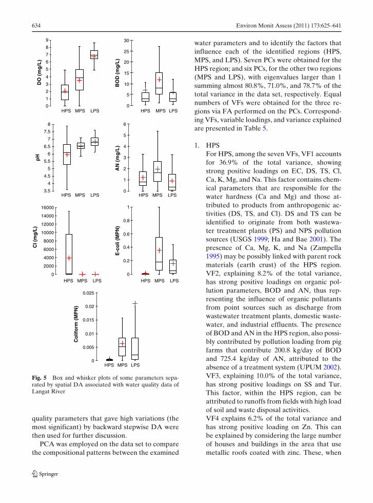
MPS, and LPS) were treated as dependent vari-ables, while water quality parameters were treatedas independent variables. DA was carried outvia standard, forward stepwise, and backwardstepwise methods. The accuracy of spatial clas-sification using standard, forward stepwise, andbackward stepwise mode DFA were 90.5% (23discriminant variables), 88.1% (six discriminantvariables), and 88.9% (seven discriminant vari-ables), respectively (Table 4). Using forward step-wise, DA, DO, BOD, pH, AN, Cl, and E. coli werefound to be the significant variables. This indicatesthat these parameters have high variation in termsof their spatial distribution. Backward stepwisemode on the other hand included coliform as theseventh parameter to have a high spatial variation.Box and whisker plots of three of these waterquality parameters over the 8-year period (1995–2002) are shown in Fig. 5. Seven selected water

Table 4 Classification matrix for DA of spatial variationsin Langat River

Sampling regions % Correct Regions assigned by DA

HPS LPS MPS

Standard DA mode (23 variables)HPS 95.65 66 1 2LPS 90.63 0 58 6MPS 87.50 2 13 105Total 90.51 68 72 113

Forward stepwise mode (6 variables)HPS 91.30 63 1 5LPS 92.19 0 59 5MPS 84.17 3 16 101Total 88.14 66 76 121

Backward stepwise mode (7 variables)HPS 91.30 63 1 5LPS 93.75 0 60 4MPS 85.00 3 15 102Total 88.93 66 76 111

634 Environ Monit Assess (2011) 173:625–641

HPS MPS LPS

HPS MPS LPS

HPS MPS LPS HPS MPS LPS

HPS MPS LPS

HPS MPS LPS

0

1

2

3

4

5

6

7

8

9D

O (

mg

/L)

LPSMPSHPS0

5

10

15

20

25

30

BO

D (

mg

/L)

3.5

4

4.5

5

5.5

6

6.5

7

7.5

8

pH

0

1

2

3

4

5

6

AN

(m

g/L

)

0

2000

4000

6000

8000

10000

12000

14000

16000

Cl (

mg

/L)

0

0.2

0.4

0.6

0.8

1

E-c

oli (

MP

N)

0

0.005

0.01

0.015

0.02

0.025

Co

lifo

rm (

MP

N)

Fig. 5 Box and whisker plots of some parameters sepa-rated by spatial DA associated with water quality data ofLangat River

quality parameters that gave high variations (themost significant) by backward stepwise DA werethen used for further discussion.

PCA was employed on the data set to comparethe compositional patterns between the examined

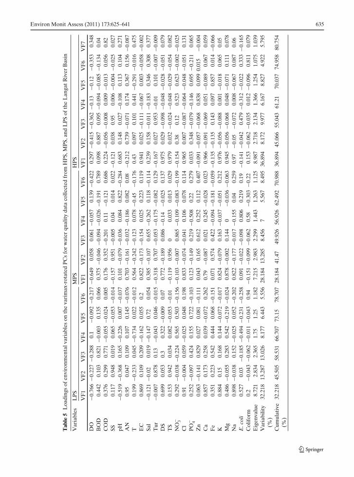
water parameters and to identify the factors thatinfluence each of the identified regions (HPS,MPS, and LPS). Seven PCs were obtained for theHPS region; and six PCs, for the other two regions(MPS and LPS), with eigenvalues larger than 1summing almost 80.8%, 71.0%, and 78.7% of thetotal variance in the data set, respectively. Equalnumbers of VFs were obtained for the three re-gions via FA performed on the PCs. Correspond-ing VFs, variable loadings, and variance explainedare presented in Table 5.

1. HPSFor HPS, among the seven VFs, VF1 accountsfor 36.9% of the total variance, showingstrong positive loadings on EC, DS, TS, Cl,Ca, K, Mg, and Na. This factor contains chem-ical parameters that are responsible for thewater hardness (Ca and Mg) and those at-tributed to products from anthropogenic ac-tivities (DS, TS, and Cl). DS and TS can beidentified to originate from both wastewa-ter treatment plants (PS) and NPS pollutionsources (USGS 1999; Ha and Bae 2001). Thepresence of Ca, Mg, K, and Na (Zampella1995) may be possibly linked with parent rockmaterials (earth crust) of the HPS region.VF2, explaining 8.2% of the total variance,has strong positive loadings on organic pol-lution parameters, BOD and AN, thus rep-resenting the influence of organic pollutantsfrom point sources such as discharge fromwastewater treatment plants, domestic waste-water, and industrial effluents. The presenceof BOD and AN in the HPS region, also possi-bly contributed by pollution loading from pigfarms that contribute 200.8 kg/day of BODand 725.4 kg/day of AN, attributed to theabsence of a treatment system (UPUM 2002).VF3, explaining 10.0% of the total variance,has strong positive loadings on SS and Tur.This factor, within the HPS region, can beattributed to runoffs from fields with high loadof soil and waste disposal activities.VF4 explains 6.2% of the total variance andhas strong positive loading on Zn. This canbe explained by considering the large numberof houses and buildings in the area that usemetallic roofs coated with zinc. These, when

Environ Monit Assess (2011) 173:625–641 635

Tab

le5

Loa

ding

sof

envi

ronm

enta

lvar

iabl

eson

the

vari

max

-rot

ated

PC

sfo

rw

ater

qual

ity

data

colle

cted

from

HP

S,M

PS,

and

LP

Sof

the

Lan

gatR

iver

Bas

in

Var

iabl

esL

PS

MP

SH

PS

VF

1V

F2

VF

3V

F4

VF

5V

F6

VF

1V

F2

VF

3V

F4

VF

5V

F6

VF

1V

F2

VF

3V

F4

VF

5V

F6

VF

7

DO

−0.7

66−0

.227

−0.2

880.

1−0

.092

−0.2

17−0

.649

0.05

80.

061

−0.0

570.

139

−0.4

220.

297

−0.4

15−0

.362

−0.1

3−0

.12

−0.3

530.

348

BO

D0.

442

0.10

30.

821

−0.0

030.

135

0.06

60.

375

−0.0

46−0

.094

−0.0

26−0

.191

0.78

90.

098

0.88

70.

095

−0.0

94−0

.085

−0.1

340.

04C

OD

0.37

60.

299

0.77

1−0

.055

−0.0

240.

005

0.17

60.

352

−0.2

010.

11−0

.121

0.68

60.

224

−0.0

56−0

.008

0.00

9−0

.013

0.05

60.

82SS

0.11

70.

948

0.01

90.

065

−0.0

53−0

.014

−0.1

570.

951

−0.0

050.

040.

014

0.02

2−0

.121

0.03

80.

950.

006

−0.0

04−0

.025

0.02

7pH

−0.5

19−0

.368

0.16

5−0

.226

0.00

7−0

.037

0.10

1−0

.079

−0.0

360.

084

0.82

2−0

.284

0.68

30.

148

0.02

7−0

.108

0.11

30.

104

0.27

1A

N0.

950.

047

0.10

90.

107

0.14

5− 0

.076

0.70

3−0

.161

−0.0

32−0

.186

0.08

20.

08−0

.212

0.73

9−0

.071

0.17

40.

367

0.15

6−0

.087

T0.

199

−0.2

330.

045

−0.7

340.

022

−0.0

120.

564

−0.2

42−0

.123

0.07

8−0

.45

−0.1

760.

430.

097

0.10

10.

441

−0.2

91−0

.016

0.47

5E

C0.

869

0.10

90.

209

−0.1

620.

055

0.2

0.82

2−0

.173

−0.1

540.

025

0.22

30.

119

0.94

10.

025

−0.1

11−0

.067

0.00

3−0

. 058

−0.0

02Sa

l−0

.121

−0.0

20.

019

−0.1

470.

720.

054

0.38

5−0

.107

0.65

5−0

.262

0.11

8−0

.114

0.23

90.

158

−0.0

11−0

.183

0.34

60.

308

0.37

7T

ur−0

.007

0.87

80.

13−0

.043

0.04

6−0

.015

−0.3

180.

707

−0.0

53−0

.175

−0.0

820.

129

−0.1

670.

027

0.95

3−0

.01

0.10

1−0

.007

−0.0

09D

S0.

699

0.05

30.

30.

322

−0.0

090.

070.

772

−0.1

890.

086

−0.1

4−0

.025

0.13

70.

975

0.02

9−0

.098

−0.0

48−0

.028

−0.0

510.

079

TS

0.15

30.

942

0.03

40.

082

−0.0

53−0

.01

−0.1

190.

956

00.

033

0.01

30.

029

0.97

90.

032

−0.0

24−0

.048

−0.0

29−0

.054

0.08

2N

O− 3

0.29

2−0

.038

−0.2

240.

565

0.50

3−0

.156

−0.1

03−0

.007

0.86

5−0

.109

−0.0

83−0

.199

−0.1

540.

380.

120.

523

0.62

3−0

.002

−0.0

25C

l0.

91−0

.004

0.05

9−0

.025

0.04

80.

198

0.83

3−0

.074

−0.0

410.

106

0.07

80.

114

0.96

50.

007

−0.0

87−0

.064

−0.0

48−0

.051

0.13

1P

O− 4

0.25

2−0

.097

0.42

40.

155

0.72

2−0

.103

0.12

3−0

.149

0.21

9−0

.508

0.22

0.27

90.

033

0.34

8−0

.079

−0.1

460.

695

−0.2

110.

065

Zn

0.06

3−0

.141

0.82

90.

027

0.08

1−0

.111

0.04

30.

165

0.61

20.

252

0.11

20.

407

−0.0

91−0

.057

−0.0

680.

838

0.09

90.

015

−0.0

04C

a0.

857

0.17

30.

258

0.03

9−0

.072

0.26

20.

79−0

.087

0.02

10.

245

−0.0

280.

023

0.96

6−0

.091

−0.0

690.

051

−0.0

890.

067

0.05

9F

e0.

351

0.22

30.

542

0.44

40.

068

−0.1

510.

071

0.57

40.

422

−0.0

94−0

.181

−0.0

59−0

.135

−0.1

350.

143

0.09

70.

857

0.01

4−0

.066

K0.

884

0.15

0.16

80.

144

−0.0

72−0

.017

0.82

4−0

.079

0.16

3−0

.037

−0.0

510.

212

0.97

6−0

.056

−0.0

880.

001

−0.0

180.

065

0.05

Mg

0.48

6−0

.055

0.28

30.

542

−0.2

19−0

.024

0.87

8−0

.002

0.14

40

−0.0

36−0

.063

0.94

5−0

.056

−0.0

680.

048

−0.0

710.

111

0.07

8N

a0.

898

−0.0

380.

152

−0.0

250.

052

−0.2

020.

822

−0.1

77−0

.017

−0.1

550.

040.

259

0.97

−0.0

5−0

.072

0.00

8−0

.067

0.08

70.

06E

.col

i0.

527

0.03

−0.1

85−0

.494

−0.2

31−0

.258

0.09

1−0

.022

−0.0

980.

806

0.21

90.

19−0

.141

−0.0

420.

479

−0.3

12−0

.022

0.33

3−0

.165

Col

ifor

m0.

2−0

.043

−0.0

62−0

.011

−0.0

430.

94−0

.151

−0.0

99−0

.062

0.58

−0.3

03−0

.22

0.15

3−0

.062

−0.0

350.

012

−0.0

960.

811

0.07

9E

igen

valu

e8.

721

2.83

42.

365

1.75

1.25

1.18

27.

215

2.98

32.

299

1.44

31.

263

1.12

58.

987

2.71

82.

134

1.36

61.

254

1.07

51.

039

Var

iabi

lity

32.2

1813

.287

13.0

268.

177

6.44

35.

556

28.1

8413

.285

8.45

67

5.56

78.

495

36.8

948.

172

9.97

76.

167

8.82

74.

922

5.79

5(%

)C

umul

ativ

e32

.218

45.5

0558

.531

66.7

0773

.15

78.7

0728

.184

41.4

749

.926

56.9

2662

.492

70.9

8836

.894

45.0

6655

.043

61.2

170

.037

74.9

5880

.754

(%)

636 Environ Monit Assess (2011) 173:625–641

in contact with acid rainwater and smog, couldreadily mobilize zinc into the atmosphereand waterways. Moderate positive loading onNO−

3 is possibly due to agricultural runoffbecause nitrogen and potassium fertilizers arecommonly used. The positive correlation ofNO−

3 and agricultural land in the HPS re-gion (located downstream) is consistent withmany others studies (Hill 1978; Neill 1989;Johnson and Gage 1997; Tufford et al. 1998).There are also weak positive and negativeloadings on T, and E. coli temperature is mostpossibly related to seasonal effects, while E.coli is strongly related to municipal sewageand wastewater treatment plants (Frenzel andCouvillion 2002) along the river in the HPSregion.VF5 explains 4.9% of the total variance andhas strong positive loading on Fe and moder-ate positive loadings on NO−

3 and PO3−4 . The

presence of Fe basically represents the metalgroup originating from industrial effluents.The presence of NO−

3 and PO3−4 are due

to agricultural runoff such as livestock wasteand fertilizers (Buck et al. 2003), indus-trial effluents, municipal sewage, and existingsewage treatment plants because PO3−

4 is animportant component of detergents (Vegaet al. 1998). VF6 explains 4.9% of the totalvariance and has strong positive loading oncoliform, while VF7 explained 5.8% of thetotal variance with strong loading on COD.These are mainly due to municipal sewage andsewage treatment plants.

2. MPSIn the case of MPS, VF1 explains 28.2% of thetotal variance and has strong loadings on AN,EC, DS, Cl, Ca, K, Mg, and Na; moderatepositive and negative loadings on temperatureand DO; weak positive loadings on BODand Sal; and weak negative loading on Tur.This first factor could be explained by con-sidering the chemical components of variousanthropogenic activities that constitute pointsource pollution especially from industrial,domestic, and commercial and agriculturalrunoff areas located at the Hulu Langat,Cheras, and Kajang districts. VF2 explains13.3% of the total variance and shows strong

positive loadings on SS, TS, and Tur, whichare related to discharge from urban develop-ment areas involving clearing of lands (USGS2007), the erosion of road edges due to sur-face runoff (Goonetilleke et al. 2005), as wellas agricultural runoff (Schlosser and Karr1981). The conversion of forest or agricul-ture land to urban areas has indeed causedlarge negative impacts to the ecosystem (Wahlet al. 1997) of Langat Basin in the formof mud flood, land slide, and river floods.Urbanization is, until now, actively pursued,in line with various developmental plans pro-posed by the government within the MPSarea (Shah et al. 2002). Moderate loadingon Fe is possibly generated from industrialactivities such as electroplating. Weak loadingon COD is related to the discharge of munici-pal and industrial waste.VF3 explains 8.5% of the total variance andshows strong positive loading on NO−

3 , mod-erate positive loading on Zn and Sal, andweak positive loading on Fe. Strong positiveloading on NO−

3 is suspected to originate fromagricultural fields (Vega et al. 1998), whereirrigated horticultural crops are grown and theuse of inorganic fertilizers (usually as ammo-nium nitrate) is rather frequent. This practicecould also explain the high levels of ammo-nia, but this pollutant may also originate fromdecomposition of nitrogen containing organiccompounds via degradation process of organicmatters (USGS 2007), such as proteins andurea occurring in municipal wastewater dis-charges. VF4 and VF5 explain 7% and 5.6%of the variance, respectively, and have strongpositive loadings on E. coli and pH, which arerelated to municipal wastes, oxidation ponds,and animal husbandry. The presence of E. coliin river water consumes large amount of oxy-gen, and as the amount of available DO de-creases, they undergo anaerobic fermentationprocesses leading to the production of am-monia and organic acids. Hydrolysis of theseacidic materials causes a decrease of waterpH values. VF6 explains 8.5% of the varianceand has strong positive loadings on BOD andCOD that, as explained before, are related toanthropogenic pollution sources and are sus-

Environ Monit Assess (2011) 173:625–641 637

pected to come from point sources pollutionsuch as sewage treatment plants and industrialeffluents.

3. LPSFinally, for the LPS region, the first VF (VF1)explains about 32.2% of the total variance andhas strong positive loadings on AN, COND,Cl−, Ca, K, and Na, and moderate positiveand negative loadings on E. coli and pH. Thepresence of AN is related to the influenceof domestic waste and agricultural runoff(Fisher et al. 2000; Osborne and Wiley 1988).McFarland and Hauck (1999), in their study,found that higher nitrogen levels were de-tected in agricultural waters, where fertiliz-ers, manure, and pesticide have been applied.Loadings on EC, Cl−, Ca, K, and Na are prob-ably due to the mineral component of the riverwater (Barnes et al. 1981; Dahlgren and Singer1994; Holloway and Dahlgren 2001). This as-sumption is reasonable, as the water qualityin this region is good and land use activitiesare mostly limited to agriculture and forestareas. Strong negative loadings on DO canbe related to high levels of dissolved organicmatter consuming large amounts of oxygen,suspected to come from agricultural activitiesand forest areas that are the dominant landuse type within this region.VF2, which explains 13.2% of the total vari-ance, has strong positive loading on SS, Tur,and TS. Lately, urban developments havebeen carried out within the LPS region (Siwaret al. 2004), and at times, especially during wetseasons, solids, especially mud, and soil fol-low runoff into the river. Agricultural runoffalso contributes toward this loading as well asconstruction. Farming and construction weremore frequent near stream areas and sedi-ment deposited as a result of these activi-ties. Thus, SS, Tur, and TS increments maybe due to overland inputs, increased stream-bank erosion, and increased entrainment ofbedload sediments during stormflow (Bolstadand Swank 1997) especially in forested area(Yusoff and Haron 1999; Yusoff et al. 2006).VF3 explains about 13% of the total varianceand has strong positive loadings on BOD,COD, and Zn. BOD and COD are considered

organic factors (Simeonov et al. 2003) andmay be interpreted as representing influencesfrom NPS such as agricultural activities andforest areas. Presence of Zn, as explained be-fore, is due to village houses with zinc roofs.VF4, VF5, and VF6, which explain about8.2%, 6.4%, and 5.6% of the total variance,respectively, have strong negative loading ontemperature and strong positive loadings onSal, PO4 and coliform. Salinity and phosphatehave their origin in soils due to the use ofphosphate fertilizers in this region as well ashigh salt content. Arheimer and Swank (2000)and Hill (1981), in their studies, concludethat agricultural land use strongly influencesstream phosphorous. The presence of col-iform is due to discharge into the river viasurface runoff of domestic waste and fertilizer(animal waste) used in agricultural activities.According to Bolstad and Swank (1997), thetransport of coliform is probably primarilythrough the soil or direct input by a warm-blooded animal (e.g., livestock). This region,formed by the Pangsoon and Ulu Lui sub-basins, is dominated by agriculture, forest, andrecreation activities along the river.

The application of WQI for river classification

The DOE started the river monitoring programsince 1978. There are 927 manual stations locatedwithin 120 river basins throughout Malaysia. Wa-ter quality data were used to determine the waterquality status and to classify the rivers basedon WQI and the Interim National Water Qual-ity Standards for Malaysia. Although WQI is aneffective tool for the purpose of monitoring, therehave been questions of its relevance in particularparameters, namely, DO, BOD, COD, AN, pH,and SS. Despite the use of AN in the WQI cal-culation, AN is not listed in the standard A and B,the Environmental Quality Acts. However, recentstudy reported that 43% of the rivers are pollutedwith AN (Hashim 2001). SS is another pollutantthat is not monitored in the DOE-approved pro-grams, but the level of SS that originated fromNPS increases during a storm event. From thecritical evaluation of the DOE data, pH has min-imal influence of the water quality. Therefore its

638 Environ Monit Assess (2011) 173:625–641

weightage in the WQI calculation should be re-duced (Azni Idris et al. 2003; Juahir et al. 2004).

Results from our study indicate that land useactivities significantly influence water quality vari-ations. Looking at the WQI, land use-based para-meters have not been considered in the equation.Taking these into consideration, we feel that tobetter classify the river, parameters should bereviewed. For example, within MPS and HPS,which industrial activity dominates, there is CODcontribution. COD exhibited positive correlation(0.82 and 0.7) for VF7 and VF6, which explainedonly 5.8% and 8.5% of the total variance for bothregions. This study agreed, as reported by Juahiret al. (2004), where upon using multiple linearregression and artificial neural networks methodsin predicting WQI at the Langat River, COD con-tributed little to the variance of the WQI. Hence,the WQI is not accurate in representing the sur-face water quality indicator for this region. WQIis less sensitive to the changes in pollutant types.Due to rapid changes in technology as well as amore diverse use of chemical, pollutant changeswith respect to space and time are more drastic.WQI, if not revised, is unable to capture thesedrastic changes. We recommended that parame-ters used in the WQI equation be revised.

Conclusions

In this study, environmetric techniques were usedto investigate the spatial variations of surface riverwater quality data of the Langat River. HACAsuccessfully classified the seven monitoring sta-tions into three different cluster regions namelyDLR, MLR and ULR. With this classification,optimal sampling strategy can be designed, whichcould reduce the number of sampling stations andassociated costs. For spatial variations, DA givesencouraging results in discriminating the sevenmonitoring station with six and seven discriminantvariables assigning 89% cases correctly using for-ward and backward stepwise modes. Applicationof the PCA coupled with the FA on the availabledata for each of the identified regions resulted inseven parameters responsible for major variationsin surface water quality along the Langat Rivercontributed by the regions (DLR, MLR, and

ULR). The main sources of variations come fromindustrial effluents, wastewater treatment plants,and domestic and commercial areas. For MLRand ULR regions, six parameters were found to beresponsible for the major variations. The sourcesof these variations at MLR are mainly attributedto industrial areas, waste water treatment plants,domestic and commercial areas, and agriculturalrunoffs. For the ULR region, the major sourceof variations mainly comes from domestic, com-mercial, agricultural runoff, and forest areas. Fora better Langat River Basin management, reviewof surface water quality changes within the devel-oping regions of MLR and DLR was compared tothat of the ULR region.

Additionally, the present WQI has some draw-backs. It is generally unable to represent the waterquality status of specifics locations. There is aneed for a holistic approach where spatial analysisis one of the most important aspects. Thus, thisstudy illustrates the of environmetric techniquesfor the analysis and interpretation of complexdata, water quality assessment, identification ofpollution sources, and investigating spatial varia-tions of water quality as an effort toward a moreeffective river basin management.

Acknowledgements The authors acknowledge the finan-cial and technical support for this project provided bythe Ministry of Science, Technology and Innovation andUniversiti Putra Malaysia under the Science Fund projectno. 01-01-04-SF0733. The authors wish to thank the De-partment of Environment and the Department of Irri-gation and Drainage, the Ministry of Natural Resourcesand Environment of Malaysia, the Institute for Devel-opment and Environment (LESTARI), the UniversitiKebangsaan Malaysia, the Universiti Malaya ConsultancyUnit (UPUM), and the Chemistry Department of Univer-siti Malaya, who have provided us with secondary data andvaluable advice.

Open Access This article is distributed under the termsof the Creative Commons Attribution Noncommercial Li-cense which permits any noncommercial use, distribution,and reproduction in any medium, provided the originalauthor(s) and source are credited.

References

Adams, M. J. (1998). The principles of multivariate dataanalysis. In P. R. Ashurst & M. J. Dennis (Eds.),Analytical methods of food authentication (p. 350).London: Blackie Academic & Professional.

Environ Monit Assess (2011) 173:625–641 639

Aiken, R. S., Leigh, C. H., Leinbach, T. R., & Moss, M. R.(1982). Development and environment in PeninsularMalaysia. Singapore: McGraw-Hill InternationalBook Company.

Alberto, W. D., Pilar, D. M. D., Valeria, A. M., Fabiana,P. S., Cecilia, H. A., et al. (2001). Pattern recognitiontechniques for the evaluation of spatial and tempo-ral variations in water quality. A case study: SquiaRiver Basin (Cordoba-Argentina). Water Research,35, 2881–2894. doi:10.1016/S0043-1354(00)00592-3.

Arheimer, P. V., & Swank, W. T. (2000). Nitro-gen and phosphorus concentrations from agriculturecatchments—Influence of spatial and temporal vari-ables. Journal of Hydrology (Amsterdam), 227(1–4),140–159. doi:10.1016/S0022-1694(99)00177-8.

Barnes, I., Kistler, R. W., Mariner, R. H., & Presser, T. H.(1981). Geochemical evidence on the nature of the base-ment rocks of the Sierra Nevada, California. U.S. Geo-logical Survey Water Supply Paper, 2181.

Bolstad, P. V., & Swank, W. T. (1997). Cumulative impactsof land use on water quality in a southern Appalachianwatershed. Journal of the American Water ResourcesAssociation, 33(2), 519–534. doi:10.1111/j.1752-1688.1997.tb03529.x.

Brodnjak-Voncina, D., Dobcnik, D., Novic, M., &Zupan, J. (2002). Chemometrics characterization ofthe quality of river water. Analytica Chimica Acta, 462,87–100. doi:10.1016/S0003-2670(02)00298-2.

Brown, S. D., Blank, T. B., Sum, S. T., & Weyer,L. G. (1994). Chemometrics. Analytical Chemistry, 66,315R–359R. doi:10.1021/ac00084a014.

Brown, S. D., Skogerboe, R. K., & Kowalski, B. R. (1980).Pattern recognition assessment of water quality data:Coal strip mine drainage. Chemosphere, 9, 265–276.doi:10.1016/0045-6535(80)90003-X.

Brown, S. D., Sum, S. T., & Despagne, F. (1996). Chemo-metrics. Analytical Chemistry, 68, 21R–61R. doi:10.1021/a1960005x.

Buck, O., Niyogi, D. K., & Townsend, C. R. (2003).Scale-dependence of land use effects on water qual-ity of streams in agricultural catchments. Environ-mental Pollution, 130, 287–299. doi:10.1016/j.envpol.2003.10.018.

Chapman, D. (UNESCO, WHO, and UNEP) (1992).Water quality assessment. London: Chapman &Hall.

Dahlgren, R. A., & Singer, M. J. (1994). Nutrient cy-cling in managed and non-managed oak woodland–grass ecosystems. Land, Air and Water ResourcesResearch Paper 100028, University of California,Davis, CA.

Department of Environment Malaysia (DOE) (1997).Malaysia environmental quality reports, 1999. KualaLumpur: Ministry of Science, Technology andEnvironment.

Department of Environment Malaysia (DOE) (1999).Malaysia environmental quality reports, 1999. KualaLumpur: Ministry of Science, Technology andEnvironment.

Department of Irrigation and Drainage (DID) (2001). DIDannual report. Kuala Lumpur.

Dixon, W., & Chiswell, B. (1996). Review of aquatic moni-toring program design. Water Research, 30, 1935–1948.doi:10.1016/0043-1354(96)00087-5.

Fisher, D. S., Steiner, J. L., Endale, D. M., Stuedemann,J. A., Schomberg, H. H., & Wilkinson, S. R. (2000).The relationship of land use practices to surface waterquality in the Upper Oconee Watershed of Georgia.Forest Ecology and Management, 128, 39–48. doi:10.1016/S0378-1127(99)00270-4.

Forina, M., Armanino, C., & Raggio, V. (2002). Clus-tering with dendograms on interpretation variables.Analytica Chimica Acta, 454, 13–19. doi:10.1016/S0003-2670(01)01517-3.

Frenzel, S. A., & Couvillion, C. S. (2002). Fecal-indicatorbacteria in streams along gradient of residential de-velopment. Journal of the American Water ResourcesAssociation, 38, 265–273. doi:10.1111/j.1752-1688.2002.tb01550.x.

Goonetilleke, A., Thomas, E., Ginn, S., & Gilbert, D.(2005). Understanding the role of land use in urbanstormwater quality management. Journal of Environ-mental Management, 74, 31–42.

Ha, S. R., & Bae, M.-S. (2001). Effects of land use andmunicipal wastewater treatment changes on streamwater quality. Water, Air, and Soil Pollution, 70, 135–151.

Hashim, D. (2001). Water pollution control in Malaysia—A regulator’s perspective. Paper Presented in theSeminar on World Day for Water, 23–24 March 2001,Batu Pahat, Johor.

Helena, B., Pardo, R., Vega, M., Barrado, E., Fernandez,J. M., & Fernandez, L. (2000). Temporal evaluationof groundwater composition in an alluvial aquifer(Pisuerga river, Spain) by principal component analy-sis. Water Research, 34, 807–816. doi:10.1016/S0043-1354(99)00225-0.

Hill, A. R. (1978). Factors affecting the export ofnitrate-nitrogen from drainage basins in southernOntario. Water Research, 12, 1045–1057. doi:10.1016/0043-1354(78)90050-7.

Hill, A. R. (1981). Stream phosphorus exports from water-sheds with contrasting land uses in southern Ontario.Water Resources Bulletin, 17(3), 627–634.

Holloway, J. M., & Dahlgren, R. A. (2001). Seasonaland event-scale variations in solute chemistry forfour Sierra Nevada catchments. Journal of Hydrol-ogy (Amsterdam), 250, 106–121. doi:10.1016/S0022-1694(01)00424-3.

Idris, A., Mamun, A. A., Mohd, A. M. S., & Wan, N. A. S.(2003). Review of water quality standards and prac-tices in Malaysia. Pollution Research, 22(1), 145–155.

Johnson, L. B., & Gage, S. H. (1997). Landscape ap-proaches to the analysis of aquatic ecosystems. Fresh-water Biology, 37, 113–132. doi:10.1046/j.1365-2427.1997.00156.x.

Johnson, R. A., & Wichern, D. W. (1992). Applied multi-variate statistical analysis (3rd ed.). Prentice-Hall Int.:New Jersey.

Juahir, H., Ekhwan, T. M., Zain, S. M., Mokhtar, M.,Zaihan, J., & Ijan Khushaida, M. J. (2008). The use ofchemometrics analysis as a cost-effective tool in sus-

640 Environ Monit Assess (2011) 173:625–641

tainable utilisation of water resources in the LangatRiver Catchment. American-Eurasian Journal of Agri-cultural & Environmental Sciences, 4(1), 258–265.

Juahir, H., Sharifuddin, M., Zain, M., Toriman, E., &Mokhtar, M. (2004). Use of artificial neural network inthe prediction of water quality index of Langat RiverBasin. Malaysia. Jurnal Kejuruteraan Awam, 16(22),42–55.

Kannel, P. R., Lee, S., Kanel, S. R., & Khan, S. P.(2007). Chemometric application in classification andassessment of monitoring locations of an urbanriver system. Analytica Chimica Acta, 582, 390–399.doi:10.1016/j.aca.2006.09.006.

Kim, J.-O., & Mueller, C. W. (1987). Introduction to factoranalysis: What it is and how to do it. Quantitative ap-plications in the social sciences series. Newbury Park:Sage University Press.

Kowalkowski, T., Zbytniewski, R., Szpejna, J., &Buszewski, B. (2006). Application of chemometricsin river classification. Water Research, 40, 744. doi:10.1016/j.watres.2005.11.042.

Liu, C. W., Lin, K. H., & Kuo, Y. M. (2003). Applica-tion of factor analysis in the assessment of ground-water quality in a Blackfoot disease area in Taiwan.The Science of the Total Environment, 313, 77–89.doi:10.1016/S0048-9697(02)00683-6.

Massart, D. L., & Kaufman, L. (1983). The interpretation ofanalytical data by the use of cluster analysis. New York:Wiley.

Massart, D. L., Vandeginste, B. G. M., Buydens, L. M.C., De Jong, S., Lewi, P. J., & Smeyers-Verbeke, J.(1997). Handbook of chemometrics and qualimetrics:Data handling in science and technology (Parts A andB, Vols. 20A and 20B). Elsevier: Amsterdam.

McFarland, A. M., & Hauck, S. L. (1999). Relating agricul-tural land uses to in-stream stormwater quality. Jour-nal of Environmental Quality, 28(2), 836–844.

McKenna, J. E., Jr. (2003). An enhanced cluster analy-sis program with bootstrap significance testing forecological community analysis. Environmental Mod-elling & Software, 18(2), 205–220. doi:10.1016/S1364-8152(02)00094-4.

Neill, M. (1989). Nitrate concentrations in river waters inthe south-east of Ireland and their relationship withagricultural practice. Water Research, 23, 1339–1355.doi:10.1016/0043-1354(89)90073-0.

Osborne, L. L., & Wiley, M. J. (1988). Empirical relation-ships between land use/cover and stream water qualityin an agricultural watershed. Journal of EnvironmentalManagement, 26, 9–27.

Otto, M. (1998). Multivariate methods. In R. Kellner, J. M.Mermet, M. Otto, & H. M. Widmer (Eds.), Analyticalchemistry. Wenheim: Wiley-VCH.

Qadir, A., Malik, R. N., & Husain, S. Z. (2007). Spatio-temporal variations in water quality of Nullah Aik-tributary of the river Chenab, Pakistan. Environmen-tal Monitoring Assessment, 140, 43–59.

Reghunath, R., Murthy, S. T. R., & Raghavan, B. R.(2002). The utility of multivariate statistical tech-niques in hydrogeochemical studies: An example from

Karnataka, India. Water Research, 36, 2437–2442.doi:10.1016/S0043-1354(01)00490-0.

Rosnani, I. (2001). River water quality status in Malaysia.In Proceedings national conference on sustainable riverbasin management in Malaysia, 13–14 November 2000,Kuala Lumpur, Malaysia.

Schlosser, I. J., & Karr, J. R. (1981). Water quality in agri-cultural watersheds: Impact of riparian vegetation dur-ing base flow. Water Resources Bulletin, 17, 233–240.

Shah, A. H. H., Hadi, A. S., & Jahi J. M. (2002).Lembangan Langat Sebagai Pentas Kehidupan. In M.Mokhtar, Shaharudin Idrus, Ahmad Fariz Mohamed,Abdul Hadi Harman Shah, & Sarah Aziz (Eds.), Lan-gat Basin research symposium 2001. Proceedings ofthe 2001 Langat Basin research symposium (pp. 9–20).Institut Alam Sekitar dan Pembangunan (LESTARI).

Shrestha, S., & Kazama, F. (2007). Assessment of sur-face water quality using multivariate statistical tech-niques: A case study of the Fuji river basin, Japan.Environmental Modelling & Software, 22, 464–475.doi:10.1016/j.envsoft.2006.02.001.

Simeonov, V., Einax, J. W., Stanimirova, I., & Kraft, J.(2002). Envirometric modeling and interpretation ofriver water monitoring data. Analytical and Bioan-alytical Chemistry, 374, 898–905. doi:10.1007/s00216-002-1559-5.

Simeonov, V., Stefanov, S., & Tsakovski, S. (2000). En-vironmetrical treatment of water quality survey datafrom Yantra River, Bulgaria. Mikrochimica Acta, 134,15–21. doi:10.1007/s006040070047.

Simeonov, V., Stratis, J. A., Samara, C., Zachariadis,G., Voutsa, D., Anthemidis, A., et al. (2003). As-sessment of the surface water quality in NorthernGreece. Water Research, 37, 4119–4124. doi:10.1016/S0043-1354(03)00398-1.

Singh, K. P., Malik, A., Mohan, D., & Sinha, S. (2004).Multivariate statistical techniques for the evaluationof spatial and temporal variations in water quality ofGomti River (India)—A case study. Water Research,38, 3980–3992. doi:10.1016/j.watres.2004.06.011.

Singh, K. P., Malik, A., & Sinha, S. (2005). Water qualityassessment and apportionment of pollution sourcesof Gomti River (India) using multivariate statisticaltechniques: A case study. Analytica Chimica Acta, 35,3581–3592.

Siwar, C., Shah, A. H. H., Hadi, A. S., Mohamed, A. F.,& Idrus, S. (2004). Socioeconomic status and transfor-mation of households in Langat Basin. In M. Mokhtar,Shaharudin Idrus & Sarah Aziz (Eds.), Ecosystemhealth of the Langat Basin. Proceedings of the 2003research symposium on ecosystem of The Langat Basin(pp. 23–43). Institut Alam Sekitar dan Pembangunan(LESTARI).

Tufford, D. L., McKellar, H. N., & Hussey, J. R. (1998).In-stream non-point source nutrient predictions withland-use proximity and seasonality. Journal of Envi-ronmental Quality, 27, 100–111.

Universiti Malaya Consultancy Unit (UPUM) (2002). Finalreport program Pencegahan dan Peningkatan KualitiAir Sungai Langat. Kuala Lumpur.

Environ Monit Assess (2011) 173:625–641 641

U.S. Geological Survey (USGS) (1999). The quality of ournation’s waters-nutrients and pesticides. U.S. Geologi-cal Survey Circular 1225.

U.S. Geological Survey (USGS) (2007). Water quality inthe Upper Anacostia River, Maryland: Continuousand discrete monitoring with simulations to estimateconcentrations and yields, 2003–05. Scientific Investi-gations Report 2007-5142, USGS, Virginia.

Vega, M., Pardo, R., Barrado, E., & Deban, L. (1998).Assessment of seasonal and polluting effects on thequality of river water by exploratory data analy-sis. Water Research, 32, 3581–3592. doi:10.1016/S0043-1354(98)00138-9.

Wahl, M. H., McKellar, H. N., & Williams, T. M. (1997).Patterns of nutrient loading in forested and urban-ized coastal streams. Journal of Experimental Ma-

rine Biology and Ecology, 213, 111–131. doi:10.1016/S0022-0981(97)00012-9.

Willet, P. (1987). Similarity and clustering in chemical in-formation systems. New York: Research Studies Press,Wiley.

Yusoff, M. K., & Haron, A. R. (1999). Water quality sta-tus of Air Hitam forest reserve. Pertanika Journal ofTropical Agricultural Science, 22(1), 127–129.

Yusoff, M. K., Ramli, M. F., Juahir, H., Mustapha, S.,Ismail, M. R., Mat Perak, Z., et al. (2006). Relation-ship between suspended solids and turbidity of riverin forested catchment. Malayan Forester, 69(1), 155–162.

Zampella, R. A. (1995). Characterization of surface waterquality along a watershed disturbance gradient. WaterResources Bulletin, 30, 605–611.