The 14th

World Conference on Earthquake Engineering October 12-17, 2008, Beijing, China

SPATIAL VARIABILITY OF NEAR FIELD GROUND MOTIONS AND ITS DESIGN IMPLICATION OF

LONG EXTENDED LIFELINE STRUCTURES NEARBY A FAULT H. Wang

1, T. Harada

2, T. Nonaka

3 , and M. Nakamura

4

1 Research Engineer, Earthquake Engineering Research Center Inc., University of Miyazaki, Miyazaki, Japan

Email:wang@eerc.co.jp 2 Professor, Dept. of Civil and Environmental Engineering, University of Miyazaki, Miyazaki, Japan

Email: harada@civil.miyazaki-u.ac.jp 3 President, Earthquake Engineering Research Center Inc., University of Miyazaki, Miyazaki, Japan

Email: nonaka@eerc.co.jp 4 Graduate Student, Dept. of Environment and Resource Sciences, University of Miyazaki, Miyazaki, Japan

ABSTRACT :

In the near field of a fault rupture, the difference in amplitude, phase, and frequency content of ground motions over extended area, “spatial variability of ground motions”, may be quite large and has an important effect on the response of extended lifelines such as long viaduct for cars or trains and also buried pipelines for water, gas, and oil etc.. However, the spatial variability of near fault ground motions has not been characterized so far in engineering field, and hence its effect on the inelastic response of lifelines nearby a fault has not been wellknown. This paper presents a theoretical method of simulating deterministically the spatial variability of near field ground motions for the purpose of seismic design and analysis of extended lifelines. The near field groundmotions with large permanent movements due to a fault are simulated using the stiffness matrix method andkinematical model of fault rupture in horizontally homogeneous layered half space. The effects of the spatial variation of ground motions upon the inelastic response behaviors of an extended viaduct and a buried pipeline, modeled by the fiber element method, are examined. It is found that the spatial variability of near field groundmotions looks like the vortexes emerging behind an obstacle in the air or water flow. It is also revealedquantitatively that the spatial variability of ground motions strongly affect on the inelastic response behaviors of the lifelines near a fault.

KEYWORDS: spatial variability of ground motions, near field earthquake ground motions, fiber element method, viaduct, buried pipelines, nonlinear seismic responses of lifeline

1. INTRODUCTION In the near field of a fault rupture, the difference in amplitude, phase, and frequency content of ground motions over extended area, that is “spatial variability of ground motions”, may be quite large and has an important influence on the response behaviors of extended lifelines such as long viaduct for cars or trains and also buried pipelines for water, gas, and oil etc.. However, the spatial variability of near fault ground motions has not been characterized so far in engineering field, and therefore its effect on the inelastic response behaviors of lifelines nearby a fault has not been well known. Study on the spatial variability of ground motions and its effect on extended lifelines has been started extensively, primarily in engineering field, at the 1970’s. So far the spatial ground motions has been characterized usually by the coherence function or the cross spectrum of the ground motions between two stations, by interpreting the recorded ground motions at several stations as a sample from the spatial and temporal stochastic processes in the stochastic field theory (Wang, 2006). In consequence, the empiricalcoherency or cross spectrum models depend on the recorded ground motions used in their estimation and also the models have perhaps not been available for the spatial variation of near field ground motions. It is, therefore, important to know the spatial variability of near fault ground motions and its effect on the inelastic

The 14th

World Conference on Earthquake Engineering October 12-17, 2008, Beijing, China response behaviors of extended lifelines near a fault. This paper presents a theoretical method of simulating deterministically the spatial variability of near field ground motions for seismic design and analysis of extended lifelines. The near field ground motions with large permanent movements due to a fault are simulated using the stiffness matrix method and the kinematical model of fault rupture in horizontally homogeneous layered half space (Harada et al., 1995, 2005). The effects of the spatial variation of ground motions upon the inelastic response behaviors of an extended viaduct and a buried pipeline, modeled by the fiber element method (Nonaka et al., 2001), are examined.

2. BRIEF DESCRIPTION OF SIMULATION METHOD OF SEISMIC WAVE FIELD BASED ON STIFFNESS MATRIX METHOD

Stiffness matrix method was originally developed by Kausel et al., (1981) and are extended to the simulation of seismic wave motions due to the kinematical fault rupture model in the multi-layered half space by Harada etal., (1999, 2005). In this chapter, a brief description of the stiffness matrix method in a Cartesian coordinatesystem is given (Harada et al., 1999, 2005). In a Cartesian coordinate system( , , )x y z , the displacement vector ( , , , ) ( , , )Tx y z t u v w=u at timet is retrieved by the three hold Fourier transform as follows,

( )( )

( )3( )1, , , , , , e

2x y

x y x yi x y tx y z t z d d dκ κ ωκ κ ω κ κ ω

π

∞ ∞ ∞

−∞ −∞ −∞

+ −= ∫ ∫ ∫u u (2.1)

in which ( ), , ,x y zκ κ ωu is the wave motion displacement vector at depth z in frequency ω and wave number ( , )x yκ κ domain. The displacement vector ( ), , ,x y zκ κ ωu can be obtained from the SH wave displacement 0( , , )v zκ ω and the P-SV wave displacements 0 0( , , ), ( , , )u z w zκ ω κ ω such as,

0 0

0 0

0

, , , ,

, , ,

( , ) ( , ) ( , )

( , , , ) ( , , ) ( , , )

( , ) ( , )

x y

x y

yx

y xx y

u z u z v z

v z u z v z

w z w z

κκκ κ ω κ ω κ ωκ κκ κκ κ ω κ ω κ ωκ κ

κ κ ω κ ω

= −

= +

=

(2.2)

where 2 2

x yκ κ κ= + stands for the wave number in the direction of wave (SH and P-SV waves) propagation. The SH wave displacement 0( , , )v zκ ω and the P-SV wave displacements 0 0( , , ), ( , , )u z w zκ ω κ ω are obtained by solving the following stiffness matrix equation (linear simultaneous equation), for example, for a three layered half space where an earthquake fault rupture occurs in the 2nd layer,

( ) ( )

( ) ( ) ( ) ( )

( ) ( ) ( ) ( )

( ) ( )

( )

( )

( )

( )

( )

( ) ( )

( ) ( )

( )

1 111 12 0 0

1 1 2 21 1 121 22 11 12

2 2 3 32 2 221 22 11 12

3 3 3 321 22

s

s

Half

z z

z z z

z z z

z z

⎛ ⎞⎛ ⎞ ⎛ ⎞⎟⎜ ⎟ ⎟⎟⎜ ⎜⎜ ⎟ ⎟⎟⎜ ⎜⎜ ⎟ ⎟⎟⎜ ⎜⎜ ⎟ ⎟+ +⎟⎜ ⎜⎜ ⎟ ⎟⎟⎜ ⎜⎟ ⎟⎜ ⎟⎜ ⎜=⎟ ⎟⎟⎜ ⎟ ⎟⎜ ⎜⎟⎜ +⎟ ⎟+ ⎜ ⎜⎟⎜ ⎟ ⎟⎟⎜ ⎜⎜ ⎟⎟⎜ ⎜⎜ ⎟⎟⎜ ⎜⎜ ⎟⎟ ⎟⎜ ⎜⎜ ⎜⎜ ⎟⎝ ⎠ ⎝ ⎠⎟+ ⎟⎜⎝ ⎠⎜ ⎟

0 0

0

0

0 0

0 0

0 0

0 0

0 0

K K u qK K K K u q q

u q qK K K Ku qK K K

⎟⎟⎟⎟⎟

(2.3)

in which 0 0( ) ( , , )z zκ ω≡u u for simplicity of notations, and ( ),nij HalfK K represent the stiffness matrix of the n-th layer and the half space, respectively. And 0( )nzq stands for the SH and P-SV wave components of theexternal forces in unit area on depth nz in frequency wave number domain. Also, the effects of the seismic

The 14th

World Conference on Earthquake Engineering October 12-17, 2008, Beijing, China waves radiated from the kinematical model of the earthquake fault rupture are expressed by the external forces ( )s nzq give by,

( )

( )

( ) ( )

( ) ( )

( )

( )

( )

( )

2 2 (2) (2)1 1 111 12

2 2 (2) (2)2 2 121 22

s

s

z z z

z z z

τ

τ

⎛ ⎞ ⎛ ⎞⎛ ⎞ −⎛ ⎞ ⎟ ⎟⎟⎜ ⎜⎜⎟⎜ ⎟ ⎟⎟⎜ ⎜⎜⎟ = −⎜ ⎟ ⎟⎟⎜ ⎜⎟ ⎜ ⎟ ⎟⎜ ⎟⎟ ⎜ ⎜⎟ ⎜⎜ ⎟ ⎟⎟⎟⎜ ⎟ ⎟⎜ ⎜⎝ ⎠ ⎝ ⎠⎝ ⎠ ⎝ ⎠

s s

s s

q K K uq K K u

(2.4)

where ( ) ( )( ), ( )n nz zτs su are the displacement and stress vectors at depthz of the SH and P-SV wave components of the seismic waves radiated from the kinematical model of the earthquake fault rupture in full space. In thesimulation of earthquake ground motions due to a fault rupture, 0( )nzq is given by zero and ( )s nzq only is used in Eqn. 2.3. The details of this method are summarized by Wang (2006). 3. CHARACTERISTICS OF SPATIAL VARIATION OF NEAR FAULT GROUND MOTIONS 3.1. Comparison of Simulated and Recorded Near Fault Ground Motions To show an ability of the theoretical simulation method (in chapter 2) used in this paper, the simulated nearfault ground motions are compared with the recorded ground motions at station 2 during the 1966 Parkfieldearthquake. In this simulation the fault-medium model by Bouchon (1979), where the extended fault rupture is modeled by a single vertical rectangular strike slip fault with the rupture velocity of 2.2 km/s and the earthmedium consists of a single sedimentary horizontal layer with thickness 1.5 km overlying a half space in which the fault rupture occurs, is slightly modified using a minimization technique of square error of the velocity ground motions. The final source parameters and earth properties used in this simulation are shown in Table 1(a) and (b). The following parameters are slightly changed from the Bouchon Model (1979) into the model usedin this paper: the thickness of the sedimentary layer, its and half space earth properties (S and P wave velocity),the rise time, and the rupture velocity. The other parameters are same to the Bouchon model.

Table 1 The source and earth medium parameters used in this simulation (a) Source parameters

Seismic moment 0M [ ]⋅N m 2.23×1010 Rise time τ [ ]s 0.3 Length of fault L [ ]km 8.5 Width of fault W [ ]km 8.5 Rupture speed rv [ ]km/s 2.6 Strike angle φ [ ] 0.0 Dip angle δ [ ] 90.0 Slip angle λ [ ] 0.0

(b) Earth medium properties

Material Properties

Thickness of layer H[ ]km

P-wave speed[ ]km/s

S-wave speed[ ]km/s

Densityρ [ ]3kg/m Q Value

1st layer 1.0 3.0 1.8 2300 100 Half space ----- 5.7 3.2 2800 400

Figure 1 shows the comparisons of the simulated and observed ground motions (the velocity and displacementmotions are calculated by integrating numerically the recorded acceleration motion in frequency domain). From Figure 1, a relatively good agreement between the simulated and recorded motions can be observed in thestrong portions of the acceleration motions as well as the displacement and velocity motions.

The 14th

World Conference on Earthquake Engineering October 12-17, 2008, Beijing, China

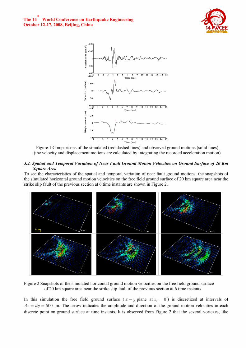
Figure 1 Comparisons of the simulated (red dashed lines) and observed ground motions (solid lines) (the velocity and displacement motions are calculated by integrating the recorded acceleration motion)

3.2. Spatial and Temporal Variation of Near Fault Ground Motion Velocities on Ground Surface of 20 Km

Square Area To see the characteristics of the spatial and temporal variation of near fault ground motions, the snapshots ofthe simulated horizontal ground motion velocities on the free field ground surface of 20 km square area near the strike slip fault of the previous section at 6 time instants are shown in Figure 2.

Figure 2 Snapshots of the simulated horizontal ground motion velocities on the free field ground surface

of 20 km square area near the strike slip fault of the previous section at 6 time instants In this simulation the free field ground surface ( x y− plane at 0 0z = ) is discretized at intervals of

500dx dy= = m. The arrow indicates the amplitude and direction of the ground motion velocities in eachdiscrete point on ground surface at time instants. It is observed from Figure 2 that the several vortexes, like

0 1 2 3 4 5 6 7 8 9 10 11 12 13 14 15600

300

0

-300

-600

Time (sec)

Acc

eler

atio

n (c

m/s

2 )

0 1 2 3 4 5 6 7 8 9 10 11 12 13 14 15100

50

0

-50

-100

Time (sec)

Vel

ocit

y (c

m/s

ec)

0 1 2 3 4 5 6 7 8 9 10 11 12 13 14 1540

20

0

-20

-40

Time (sec)

Dis

pla

cem

ent

(cm

)

The 14th

World Conference on Earthquake Engineering October 12-17, 2008, Beijing, China those appearing behind an obstacle in an air or water flow, appear around the projection line of the fault rupture (center line portion of the 20 km square area ) in the near fault ground motion velocities, and then the spatialvariability of motions is significant. It should be noted that such the spatial variation of near fault groundmotions may be reemerged from the recorded ground motions, but the simulation method as the presented one can be used as an efficient and powerful tool to specify the spatial variation of near fault ground motions takeninto account for not only the site condition but also the type of fault rupture. 4. SPATIAL AND TEMPORAL RESPONSE VARIATION OF AN IDEALIZED CONTINUOUS

VIADUCT NEAR A STRIKE SLIP FAULT To see a spatial and temporal response variation of the extended lifelines near a fault, an idealized continuous viaduct model, having entire length of 8040 m with each span length of 60 m, is used in this numericalexample. Figure 3 shows a plan view of the location of the projection line of the strike slip fault of the previouschapter 3, and of the pier’s number of the idealized continuous viaduct along the fault. (a) Plane view (b) Cross sectional view

Figure 3 Coordinates and location of the piers of continuous viaduct, and of the projection line of the strike slip fault of the previous chapter 3

Figure 4 shows the cross section of the pier of the idealized continuous viaduct. For all 135 piers, the idealizedcontinuous viaduct has the same cross section as shown in Figure 4. The piers are rigidly supported at the bottom by assuming the viaduct is situated on rock site. The piers are made of steel with rectangle cross sectionand fulfilled by concrete at the bottom portion of pier. The dimension and the material properties of the pier andthe viaduct are indicated in Table 2. Figure 4 Transverse cross section of the idealized Figure 5 Discrete model of the idealized viaduct

viaduct used in this numerical example used in this numerical example

(Rupture Propagation)

L=8500m

1 2 3 67 135

2520m

Y

X

v

uw

8040m

180m

10560m

(Fault) 180m

No67Pier

Fault

Ground Surface

The 14th

World Conference on Earthquake Engineering October 12-17, 2008, Beijing, China

Table 2 Dimension and material properties of the viaduct and pier (a) Dimension of the idealized continuous viaduct used in this numerical example

Number of piers 135 Length of span [ ]m 60.0 Height of pier [ ]m 13.0 Height of C.G of deck [ ]m 15.764 Height of concrete fulfilled portion [ ]m 3.65 Total length of viaduct [ ]m 8040

(b) Dimension of the pier of idealized continuous viaduct used in this numerical example Width[ ]mm Thickness[ ]mm Rib[ ]mm Number of panel Flange 2700 33 270×26 5 Web 3066 33 270×26 6

(c) Material properties of the pier used in this numerical example Densityρ [ ]3kN/m Shear modulus G[ ]2N/mm Yield stress yσ [ ]2N/mmSteel (SM520) 76.93 8.1×104 360 Concrete 21.56 1.02×104 21

The piers are modeled by the 3 dimensional fiber element model (Nonaka et al., 2001) where the two directional bending moments can be taken into consideration in the inelastic response analysis of the piers. Thedeck superstructures are modeled by the 3 dimensional elastic frame and they are supported by the rubbershoes, which also are modeled by elastic spring. Finally the idealized continuous viaduct is discretized by 3234frame elements with 3101 lumped masses as shown in Figure 5.

Figure 6 Snapshots of the inelastic seismic response displacements of viaduct at 6 time instants (Deformation scale: 10.0)

The inelastic responses of the viaduct are computed by the 3 dimensional fiber element method (Nonaka et al.,

1.0sec

2.0sec

3.0sec

4.0sec

5.0sec

6.0sec

The 14th

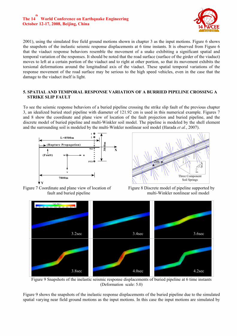
World Conference on Earthquake Engineering October 12-17, 2008, Beijing, China 2001), using the simulated free field ground motions shown in chapter 3 as the input motions. Figure 6 showsthe snapshots of the inelastic seismic response displacements at 6 time instants. It is observed from Figure 6 that the viaduct response behaviors resemble the movement of a snake exhibiting a significant spatial and temporal variation of the responses. It should be noted that the road surface (surface of the girder of the viaduct)moves to left at a certain portion of the viaduct and to right at other portion, so that its movement exhibits the torsional deformations around the longitudinal axis of the viaduct. These spatial temporal variations of theresponse movement of the road surface may be serious to the high speed vehicles, even in the case that thedamage to the viaduct itself is light. 5. SPATIAL AND TEMPORAL RESPONSE VARIATION OF A BURRIED PIPELINE CROSSING A

STRIKE SLIP FAULT To see the seismic response behaviors of a buried pipeline crossing the strike slip fault of the previous chapter3, an idealized buried steel pipeline with diameter of 121.92 cm is used in this numerical example. Figures 7and 8 show the coordinate and plane view of location of the fault projection and buried pipeline, and the discrete model of buried pipeline and multi-Winkler soil model. The pipeline is modeled by the shell element and the surrounding soil is modeled by the multi-Winkler nonlinear soil model (Harada et al., 2007). Figure 7 Coordinate and plane view of location of Figure 8 Discrete model of pipeline supported by

fault and buried pipeline multi-Winkler nonlinear soil model

Figure 9 Snapshots of the inelastic seismic response displacements of buried pipeline at 6 time instants

(Deformation scale: 5.0) Figure 9 shows the snapshots of the inelastic response displacements of the buried pipeline due to the simulated spatial varying near field ground motions as the input motions. In this case the input motions are simulated by

(Rupture Propagation)

L=8500m 21

961

1921

7800m

Y

X

v

uw

3840

m

(Fault)

Three Component Soil Springs

2m

3.2sec 3.4sec 3.6sec

3.8sec 4.0sec 4.2sec

The 14th

World Conference on Earthquake Engineering October 12-17, 2008, Beijing, China using the thickness of the 1st layer 0H = km in Table 1. The collar contour indicates the yield ratio ( max yield/σ σ ) of induced maximum stress in pipeline. It is observed from Figure 9 that the abrupt change of response displacements of buried pipeline occurs at the portion crossing the fault, and the maximum response displacements (induced stress takes maximum) occurs at time 4.0 sec., which is larger than those due to the permanent ground movement after time 4.2 sec.. 6. CONCLUSIONS A theoretical method is presented to simulate deterministically the spatial variation of near field (fault) groundmotions for seismic design and analysis of extended lifelines near a fault. By using the simulated spatial varying near field ground motions as the input ground motions, an inelastic response analysis of extended lifelines neara fault is carried by making use of the 3D fiber element method. The presented theoretical method can take into account for the following important factors in seismic design and analysis of extended lifelines: the effect of extended fault rupture, the effect of seismic wave propagation in multi-layered half space, the effect of nonlinear soil foundation interaction, the effect of inelastic response of multiple supported lifelines. Three numerical examples based on the presented theoretical method are presented: the first example is the spatial variation of the near field ground motions near a strike slip fault, the second and third example are the spatialvariation of inelastic response of an idealized continuous viaduct and a buried pipeline near a fault by using the spatially varying near field ground motions as the input ground motions. These numerical examples showquantitatively a unique spatial variation of near field ground motion like vortexes, and also its strong influenceon the inelastic response behaviors of extended lifelines near a fault.

REFERENCES Bouchon, M. (1979). Predictability of ground displacement and velocity near an earthquake fault, an example:The Parkfield Earthquake of 1966, Journal of Geophysical Research, 84, B11, 6149-6156. Harada, T., Ohosumi, T., and Okukura, H. (1999). Analytical solutions of wave field in 3-dimensional Cartesian coordinate and their application to synthesis of seismic ground motions, Journal of Structural Mechanics and Earthquake Engineering, Japan Society of Civil Engineers, 612/I-46, 99-108. Harada, T. and Wang, H. (2005). Stiffness matrix based representation of wave motions in horizontally layered media, ZISIN, The Seismological Society of Japan, 57, 387-392. Harada, T., Nonaka, T., Magoshi, K., Iwamura, M., and Wang, H. (2007). A nonlinear dynamic soil-foundation interaction model using fiber element and its application to seismic response analysis of bridge. Journal of Applied Mechanics, Japan Society of Civil Engineers (JSCE), 10, 1047-1054. Kausel, E. and Roesset, J.M. (1981). Stiffness matrices for layered soils. Bull. of Seismological Soc. of America, 71, 1743-1761. Nonaka,T. and Ali, A. (2001). Dynamic response of half-through steel arch bridge using fiber model. Journal of Bridge Engineering, American Society of Civil Engineering (ASCE), 6, 482-488. Wang, H. (2006). Theoretical method for characterization of near fault wave motion and response of extendedstructures, PhD thesis, University of Miyazaki, Miyazaki, Japan. http://ir.lib.miyazaki-u.ac.jp/dspace/handle/123456789/674