Spatial structure of disordered media: Unravelling the mechanical significance of

disorder in granular materials

K.P.Krishnaraj

Department of Chemical Engineering, Indian Institute of Science, Bangalore, India

e-mail: krishnarajkp@gmail.com

Abstract

For two decades now, the importance of microstructure in the mechanical behaviour of a large

collection of grains has been a topic of intense research1-16. Many approaches have been

developed to study the microstructure in granular materials, based on local or mesoscopic

measures3,6,8-11 or using ideas from diverse fields like percolation theory7,12, complex

networks7,13,14 and persistent homology15,16. However, we do not fully understand the role of

microstructure in the mechanical behaviour of simple and commonplace packings like a pile

of sand2,17-26 or box of grains1,2,7,17,27,28. Here, by characterizing the spatial variation of local

microstructure, we uncover intriguing large-scale spatial patterns in particle packings deposited

under the influence of gravity. We detail the emergence of these patterns, and provide a unified

fundamental explanation of classic and puzzling mechanical behaviours of granular materials

like central stress minimum2,17-26 and Janssen effect7,27,28. Further, we show the striking

dependence of spatial structure on the history of preparation, size distribution of particles and

boundary conditions. Our study reveals the existence of global spatial structure in a locally

disordered media, and elucidates its significance in the mechanical behaviour of granular

materials.

Introduction

Particulate media are a common form of matter that we encounter in our daily lives. Granular

materials are important and more familiar representative of particulate media, considering their

prevalence in nature and relevance in processing industries1,2,17. Also, force transmission in

granular media is strikingly similar to other particulate media like foams29, emulsions30,31,

gels32,33, and even bacterial suspensions34. However, the mechanical behaviour of even the

simplest of geometries like a pile2,17-26 or a vertical column of grains1,2,7,17,27,28 has proved to be

challenging to model and, no general explanation is available1,2,17. In granular piles created by

pouring grains from a narrow source like a funnel, the normal stress at the base exhibits a local

minimum beneath the apex2,17-26, in contrast to intuitive expectation. And, in a vertical column

of grains filled by raining, the components of wall stress asymptotically saturate with depth

from the free surface, commonly referred to as the Janssen effect7,27,28. Some studies suggest

that the microstructure might be the cause of central stress minimum in granular piles21-25,35-38,

but the evidences are not conclusive. In a granular column though, the role of microstructure

in Janssen effect is unclear and has not been studied in detail before7,28. Many explanations of

these mechanical anomalies have been proposed7,27,35-43, but a generally accepted consensus is

yet to be reached1,2,17,43. Further, these intriguing mechanical behaviours have inspired

numerous studies on the microstructure of granular materials3-16.

Our current understanding of the microstructure of granular materials is based on local particle

scale measures like the contact vector orientations3,6 or mesoscopic structures made of

particles8-10 or force chain orientations11,23,24 (also mesoscopic) or percolation analysis of the

contact force network7,12 or complex network measures7,13,14 like communities14 or topological

invariants like Betti numbers15,16. In a recent study, the need and advantages of a long-ranged

measure of microstructure over the existing local particle scale or mesoscopic approaches was

shown7. A comprehensive and generally accepted description of the microstructure in granular

materials is yet to be found. Hence, in modelling force transmission through granular materials,

the details of the microstructure are not adequately represented. For example, in the widely

studied q model of force transmission44, the effects of contact angles of particles are chosen

from a common distribution without regard to the spatial position, and the model does not

explain the central stress minimum in piles or Janssen effect in silos. However, anisotropic

extensions of the q model can predict the central stress minimum in granular piles41. In addition,

some studies on the microstructure of granular piles show that, contact vector distributions

considerably differ depending on the geometric region of the pile studied25. In point force

experiments too, the spatial ordering of the packing was shown to influence force

transmission4,5. Further, some continuum models that account for structural anisotropy based

on intuitive ideas like arching do predict the central stress minimum35-38. Hence, the spatial

dependence of microstructure in granular materials is important and is not well understood.

In this work, using a simple yet novel method to characterise the spatial variation of local

microstructure, we reveal striking spatial patterns in granular packings under gravity, and

provide a unified explanation to central stress minimum in piles and Janssen effect in silos. We

show that, the spatial structure in granular piles surprisingly emerges from a nearly horizontal

flow in the core region, in complete contrast to surface avalanches hypothesis of many previous

studies21-25,35-38,41,42. Further, we show that, the spatial structure can vary dramatically

depending on the method of deposition, boundary conditions and size distribution of the

particles. The details of the simulation method, various systems studied and deposition

procedure used for creating pile and silo packings are provided in Supplementary Note 1 & 2.

Results and discussion

First, we describe a method to qualitatively present the spatial pattern of the contact network.

In packing’s deposited only under the influence gravity, the weight is transmitted in a preferred

direction i.e. the direction of gravity. Hence, we find the average orientation of contacts in the

direction of gravity and their spatial distribution. From every particle centre, we define a vector,

�⃗� based on the resultant direction of its contacts, here we only consider contact directions with

a positive vertical component in the direction of gravity (see Fig. 1). For example, in Fig. 1,

from particle A, a contact A-B is considered only if �⃗� 𝑎𝑏 . 𝑔 > 0, where �⃗� 𝑎𝑏 is the normalized

contact vector and 𝑔 is a unit vector in the direction of gravity. Thus, for every particle, a vector

is assigned, and a vector field is obtained for the complete packing. The resulting vector field

is also averaged over many independent realizations. Then, like the streamlines of a continuum

velocity field, we draw lines that represent the local direction of the contact vector field at every

spatial point. We refer to this representation of the contact network as contact lines of the

packing.

Figure 1: Definition of �⃗⃗� . For particle A (coloured in blue), only contacts vectors �⃗� 𝑎𝑖, with �⃗� 𝑎𝑖 . 𝑔 > 0 (shown

in grey) are considered for finding �⃗� (shown in red), where 𝑔 is the unit vector in the direction of gravity, and 𝑖 is

the index of all particles in contact with A.

Now, we describe the spatial structure of pile and silo packings using contact lines. As shown

in Fig. 2,3, emergence of large-scale spatial pattern in the contact network is clear in the contact

line representation. In piles created by narrow source deposition method (Fig. 2a, b), along the

vertical height of the pile, the contact lines are directed away from the centre. In contrast, the

contact lines in piles created by raining particles are aligned almost vertically along the

direction of gravity (Fig. 2a, b). Hence, load transmission through the contact lines would result

in the local stress minimum beneath the apex of narrow source deposited piles. The existence

of such preferred directions of propagation explains why some phenomenological yet insightful

continuum models35-38,41 can predict the stress dip in granular piles. Interestingly, in piles

deposited from a narrow source but with monodisperse particles, the contact lines are

remarkably different compared to the polydisperse case (Fig. 2c) and vertical orientation of the

contact lines in the core regions explains the absence of central stress minimum reported in

previous studies40,45,46. In silos with frictional walls, the contact lines show a clear curvature

towards the lateral walls (Fig. 3a, c). And, in silos made up of smooth frictionless walls but

with frictional particles where the Janssen effect is absent, the contact lines are almost vertically

oriented in the direction of gravity (Fig. 3b). Hence, in silos with frictional walls, load

transmission along the contact lines would result in the vertical load screening effect with depth

i.e. Janssen effect7,27,28. Later, using a simple model of force transmission, we corroborate the

claims we have made above, and directly relate the contact lines to the stress anomalies

observed in pile and silo packings. We also find that, the contact line patterns are independent

of the type of contact model used, various particle-particle interaction parameters, and

deposition procedure (see Supplementary Note 2). Hence, the contact line representation is a

useful qualitative measure to understand the spatial structure in granular media. Next, we

discuss the emergence of these spatial patterns in detail by studying the time evolution of pile

and silo packings.

(a) (b)

(c) (d)

(e) (f)

Figure 2: Spatial structure of granular piles. Contact lines of 2d and 3d piles. (a) 2d piles, deposited from a

narrow source. (b) 2d piles, deposited by raining. (c) 3d piles, deposited from a narrow source. (d) 3d piles,

deposited by raining. (e) 2d pile of monodisperse particles deposited from a narrow source. In all cases, dashed

lines represent the average height of the free surface. (f) Orientation distribution of �⃗� (Fig. 1) in 2d piles, here we

have considered only the core region of the right-hand side of the pile. The core region is defined as particles

within 𝑟 = 0 and 𝑟 = 0.3𝑅, where, 𝑅 is the half width of the pile. The details of the system and number of

configurations studied are given in Supplementary Note 2.

(a) (b) (c)

Figure 3: Spatial structure of granular silos. Contact lines of 2d and 3d silos. (a) Contact lines of 2d silos with

rough frictional walls. (b) Contact lines of 2d silos with smooth frictionless walls, but the particles are frictional.

(c) Contact lines of 3d silos with rough frictional walls. In all cases, dashed lines represent the average height of

the free surface, and the width of the silos, 𝑊𝑠 = 20𝑑𝑝 and the average height of the free surface, 𝐻𝑠 ≈ 12𝑊𝑠.

The details of the system and number of configurations studied are given in Supplementary Note 2.

In piles, the streamlines of the displacement field of particles reveal interesting patterns of

evolution depending on the method of deposition (see Supplementary Video 6-8) (details of

Supplementary Videos are given in Supplementary Note 4). In narrow source deposited piles,

we find a strong horizontal outward flow from the centre (see Supplementary Video 6) and in

rained piles, a perceptible flow is observed only along the surface (see Supplementary Video

7). We also studied the evolution of piles by sequentially labelling the particles based on their

time of deposition (see Supplementary Video 1,2), in narrow source deposited piles, the spread

of newly deposited layers of particles in the horizontal direction due to the outward flow can

be clearly seen. In addition, the time evolution of the contact lines also correlates well with the

layering patterns induced by the nearly horizontal flow (see Supplementary Video 1). Hence,

the strong horizontal component of the particle flow at the apex of the pile results in noticeable

anisotropy in the core region of the pile (Fig. 2d), which is preserved in subsequent layers of

newly deposited particles. Such changes in microstructure caused by externally imposed shear

or deformation in granular media is well known3,5,6,7,42. Also, recent continuum modelling and

discrete simulation studies find strong anisotropy in the core region of the pile as suggested by

our results25,43 (Fig. 2d). We note that, the above conclusion is in complete contrast to the

surface avalanches hypothesis suggested by many previous studies21-25,35-38,41,42. Curiously, we

find that, the emergence of structural pattern in monodisperse piles is primarily driven by

surface avalanches (see Supplementary Videos 3,8) and is remarkably different compared to

the polydisperse case. Though local ordering or crystallization effects are important in

monodisperse packings47,48, here we have shown that, surface avalanches in granular piles can

lead to a maximum of stress beneath the apex.

The emergence of the spatial order in silos is also interesting, we explain this by studying the

evolution of the displacement field of the particles and the contact lines (see Supplementary

Videos 4,5,9,10). In silos with frictional walls, the spatial order emerges from particle

rearrangements near the growing free surface. We find clear particle movements towards the

lateral walls in the growing free surface region of the packing (see Supplementary Video 9).

The microstructural rearrangements caused by the surface flow is reflected in the evolution of

contact lines with time (see Supplementary Video 4). However, in silos made of smooth

frictionless walls but with frictional particles, in addition to particle movements towards the

lateral walls in the growing free surface region, we find slow and continuous nearly vertical

flow along the entire height of the column (see Supplementary Video 10). The time evolution

of particle displacements and contact lines clearly suggests that, the slow continuous vertical

flow determines the microstructure of the packing in the final static state (see Supplementary

Video 5,10). Hence, we conclude that, frictional resistance of the lateral walls hinders the slow

vertical flow, and particles movements towards the lateral walls in the growing free surface

region determine the spatial structure. We next show how the observed structural patterns can

help us understand central stress minimum and Janssen effect, using a simple model of force

transmission. It is important to note that, here we do not attempt to develop an exact model of

force transmission, our aim is only to show the effect of spatial structure on the mechanical

response of granular materials.

We use the simplest possible model of force transmission in granular materials i.e. the weight

of the particle is assumed to be transmitted to the supporting base by a random walk. As the

information of spatial structure is unknown, we use the information of the contact network

from DEM generated packings in the random walk studies. Our objective here is to show that,

only the information of the contact network (or the spatial structure of it) can be used to explain

the central stress minimum and Janssen effect in granular media, using a force transmission

model as simple as a random walk. Here, the random walk can propagate only in the direction

of gravity; we refer to this as the Random Walk (RW) model. In RW, the weight of a bulk

particle is transmitted to the supporting base (boundary particles) through random paths (see

Methods section for details), and the fraction of the total weight of the pile reaching a boundary

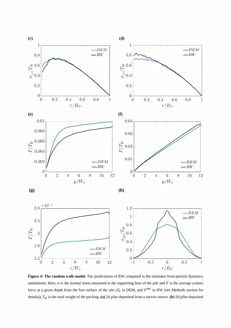
particle is found and is averaged over many independent realizations. Though the random walk

is an oversimplified model of force transmission, remarkably it predicts the central stress

minimum in piles reasonably well for polydisperse piles (Fig. 4a-d). Interestingly, we find that

the RW predictions in piles made up of particles with large spring stiffness values or Hertz

spring are in very close agreement with DEM results (see Supplementary Figures 7,8), which

further suggests that the RW is a reasonable model of force transmission in realistic granular

piles. However, in monodisperse piles, though the RW explains the presence of a maximum of

stress beneath the apex similar to DEM estimates, a close agreement, as observed in

polydisperse piles, is lacking (Fig. 4h), the reason is unclear to us, but can be caused by local

ordering or crystallization effects47,48 as discussed before. We base our above claim on point

force experiments on 2d disk packings4,5, where force transmission in ordered packings was

shown to be dramatically different compared to disordered packings. Next, to the show the

effect of spatial structure on RW prediction in silos, we compare packings with frictional and

frictionless walls. As shown in Fig. 4e,g, the RW in the frictional wall-bounded silo packing

shows strong signatures of Janssen saturation compared to packings with smooth frictionless

walls (Fig. 4f), this can be better understood by contrasting the spatial structures of the packings

(Fig. 3a,b). We note that, load transfer due to frictional interactions are important in wall-

bounded packings like silo17,27,49, and RW does not account for friction between particles,

hence we do not observe a close agreement between RW and DEM predictions in the silo with

frictional walls compared to the frictionless case. The effect of wall roughness and width of

silo are discussed in Supplementary Note 2.

(a) (b)

(c) (d)

(e) (f)

(g) (h)

Figure 4: The random walk model. The predications of RW compared to the estimates from particle dynamics

simulations. Here, σ is the normal stress measured at the supporting base of the pile and 𝐹 is the average contact

force at a given depth from the free surface of the silo (𝐹𝑛 in DEM, and 𝐹𝑅𝑊 in RW (see Methods section for

details)), 𝑇𝑊 is the total weight of the packing. (a) 2d piles deposited from a narrow source. (b) 2d piles deposited

by raining. (c) 3d piles deposited from a narrow source. (d) 3d piles deposited by raining. (e,f) 2d silos with rough

frictional walls (e) and smooth frictionless walls (f). (g) 3d silos with rough frictional walls. (h) 2d piles made up

of monodisperse particles deposited from a narrow source. The averaging procedure and number of configurations

studied are given in Supplementary Note 2.

To clearly show how a random walker’s movement is determined by the spatial structure of

the packing? We now compare the average trajectories of random walks with contact lines. In

RW, the total weight transmitted through a contact (𝐹𝑅𝑊) can be found (see Methods section

for details). Hence, each contact can be weighted by 𝐹𝑅𝑊, and we define the vector field based

on the weighted contact vectors. We then construct streamlines based on weighted contact

vector field and refer to this as random walk lines (see Supplementary Note 4). As expected,

the random walk lines agree almost exactly with contact lines (see Supplementary Fig. 11).

Interestingly, in granular piles made up of polydisperse particles, we also find that, streamlines

based on contact vectors weighted by the normal contact force (𝐹𝑛), are also in close

agreement with the contact lines (see Supplementary Fig. 12a-d), and we refer to this as force

lines. It is important to note that, in the random walk model, the direction of movement is

independent of the direction of the previous step (spatially uncorrelated). Hence, long-ranged

structural correlations or force chains or arches are mechanically not significant in the

emergence of central stress minimum in granular piles, unlike previously thought21-24,35-38.

However, in monodisperse piles, as suggested by the RW predictions, we find that the force

lines and contact or random walk lines are similar only the core region, and show drastic

difference away from the centre (see Supplementary Fig. 12e). In silos too, we find that the

contact lines and random walk lines agree almost exactly (see Supplementary Fig. 11f-h), and

as explained before, the force weighted contact lines show stronger curvature compared to the

contact lines due to frictional interactions of particles with lateral walls (see Supplementary

Fig. 12f-h). Hence, using only the information of the contact network and with random walk

as a model of force transmission, we have clearly shown the significance spatial variations of

local microstructure on some curious cases of mechanical behaviour in granular materials.

Finally, we discuss how the information of spatial structure can be used in modelling force

transmission in granular piles.

As explained previously, in the case of granular piles, the RW is a useful model of force

transmission. Hence, we explain how the spatial structure can be represented in the continuum

analogue of the RW. In the continuum limit, the RW resembles the drift-diffusion equation50,51

(see Methods). The transmission of the weight of a grain or applied load (𝑊) is given by,

∂𝑊

∂𝑡= −∇. (𝐯𝑊) + ∇. (∇(𝐃𝑊)) (1)

Where, time (𝑡) represents the spatial coordinate (𝑦 in 2d and 𝑧 in 3d) in the direction of

gravity, 𝑔 . Here, the information of the spatial structure is represented by spatially varying,

drift rate, 𝐯(𝑥, 𝑦) and diffusion constant, 𝐃(𝑥, 𝑦). The functions 𝐯(𝑥, 𝑦) and 𝐃(𝑥, 𝑦) are

difficult to find, only in the simplest of cases, as in a rained pile of grains (Fig. 2b,d) or a silo

packing with frictionless walls (Fig. 3c) can be modelled as spatially homogenous.

Conclusion

By visually presenting the spatial variation of local microstructure of the complete packing, we

have shown the existence of large-scale spatial structure in granular media. Based on the spatial

structure of pile and silo packings, we have provided fundamental explanations to some long

standing and puzzling mechanical behaviours in granular media. Moreover, we have shown

that, the spatial structure can vary dramatically depending on the method of deposition,

boundary conditions and size distribution of particles, and consequently the mechanical

behaviour too. The mechanical significance of spatial structure in other disordered media like

foams, emulsions and even biological populations are worth investigating.

Acknowledgements

I sincerely thank Professor Prabhu R Nott for insightful discussions and useful critiques. I am

profoundly grateful to N.Marayee, P.Rajamani, K.P.Dhanasekaran, A.K.K.Arvind and Mani

for their encouragement and support. I also thank R.S.Veeraraahavan and S.Karthick for their

hospitality.

Methods

1. Random walk model

In the random walk model, the weight of individual particles is transmitted to the boundaries

through contacts by a random walk. Here, we only choose contact directions with a positive

vertical component in the direction of gravity. From every particle, numerous paths (through

the contact network) are possible for a random walk to reach the supporting base. And,

enumerating all possible paths reaching the supporting base is computationally prohibitive.

Hence, in this study, we use a statistical approach, we randomly sample a subset of all possible

paths with 𝑅𝑊𝑖 random walks from the given bulk particle, 𝑖. The fraction of the weight of a

bulk particle 𝑖 transmitted to a boundary particle 𝑗, 𝐹𝑖𝑗 is given by,

𝐹𝑖𝑗 =𝑅𝑊𝑗

𝑖 × 𝑊𝑖

𝑅𝑊𝑖(2)

Where, 𝑊𝑖 is the weight of a bulk particle 𝑖 and 𝑅𝑊𝑗𝑖 is the number of random walks reaching

a boundary particle 𝑗 starting from a bulk particle 𝑖.

Hence, in a pile made up of 𝑁 particles, the fraction of the total weight of the pile supported

by a boundary particle 𝑗, 𝐹𝑗𝑅𝑊 is given by,

𝐹𝑗𝑅𝑊 = ∑

𝑅𝑊𝑗𝑖 × 𝑊𝑖

𝑅𝑊𝑖

𝑁

𝑖=1

(3)

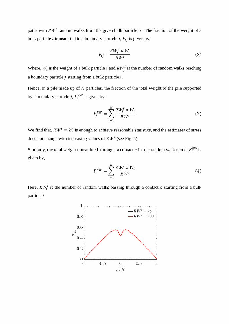
We find that, 𝑅𝑊𝑖 = 25 is enough to achieve reasonable statistics, and the estimates of stress

does not change with increasing values of 𝑅𝑊𝑖 (see Fig. 5).

Similarly, the total weight transmitted through a contact 𝑐 in the random walk model 𝐹𝑐𝑅𝑊is

given by,

𝐹𝑐𝑅𝑊 = ∑

𝑅𝑊𝑐𝑖 × 𝑊𝑖

𝑅𝑊𝑖

𝑁

𝑖=1

(4)

Here, 𝑅𝑊𝑐𝑖 is the number of random walks passing through a contact 𝑐 starting from a bulk

particle 𝑖.

Figure 5: The effect of number of paths (𝑅𝑊𝑖) sampled randomly for a bulk particle. We find that, for

every bulk particle 𝑖, 𝑅𝑊𝑖 = 25 is a sufficient, and increase in the number of paths sampled does affect

the RW predictions.

2. Continuum approximation of the random walk model in disordered media

Figure 6: Schematic of a random walker moving through a disordered packing in the direction of

gravity. Here, 𝑔 is the unit vector in the direction of gravity.

We model force transmission in granular materials as a random walker moving through a

disordered lattice. At each time step τ, the random walker can move a distance δ (≈ 𝑑𝑝) in one

of the 𝑁 possible directions given by 𝜃𝑖, where 𝜃𝑖 ∈ {𝜃1, 𝜃2, 𝜃3 …𝜃𝑁} and {0  ≤  𝜃𝑖   < 2𝜋}50.

The probability of transition, which depends on the current position (𝑥, 𝑦) is given by 𝑃𝑖(𝑥, 𝑦),

and ∑ 𝑃𝑖(𝑥, 𝑦)𝑁𝑖=1 = 1. Here, we consider forward progression in time (𝑡) as movement in

space along the direction of gravity, 𝑦 in 2d and 𝑧 in 3d. The weight of a grain (𝑊) at position

(𝑥, 𝑦) after a forward time step is given by50,

𝑊(𝑥, 𝑦, 𝑡) = ∑(𝑊(𝑥  −  δ𝑠𝑖𝑛(𝜃𝑖), 𝑦  −  δ𝑐𝑜𝑠(θi), 𝑡  − τ)𝑝𝑖(𝑥  −  δ𝑠𝑖𝑛(θi), 𝑦 

𝑁

𝑖=1

−  δ𝑐𝑜𝑠(𝜃𝑖)))

+𝑊(𝑥, 𝑦, 𝑡  −  τ) (1  −  ∑𝑝𝑖(𝑥, 𝑦)

𝑁

𝑖=1

) (4)

As shown in chapter 2 of reference 50, in the continuum limit i.e., δ and τ → 0, the above

equation can be written as,

∂𝑊

∂𝑡= −∇. (𝐯𝑊) + ∇. (∇(𝐃𝑊)) (5)

Where, 𝐯(𝑥, 𝑦) and 𝐃(𝑥, 𝑦) are spatially varying drift rate and diffusion constant respectively.

And are given as,

𝐯 = (𝑣1

𝑣2) 𝑎𝑛𝑑 𝐃 = (

𝑑11 𝑑12

𝑑12 𝑑22) (6)

Equation (5) is reminiscent of the two-dimensional drift-diffusion equation50,51. Here, the drift

rate and diffusion coefficient depend on the spatial position, typically unknown functions, and

are described by the contact lines in Fig. 2. Hence, given the information of local microstructure

of the packing, 𝐯(𝑥, 𝑦) and 𝐃(𝑥, 𝑦), the base stress distribution in gravity deposited granular

piles can be predicted using equation (5).

References

1. Jaeger, H. M., Nagel, S. R., & Behringer, R. P. Granular solids, liquids, and gases. Rev.

Mod. Phy. 68, 1259 (1996).

2. de Gennes, P. G. Granular matter: a tentative view. Rev. Mod. Phy. 71, S374 (1999).

3. Radjai, F., Wolf, D. E., Jean, M., & Moreau, J. J. Bimodal character of stress

transmission in granular packings. Phy. Rev. Lett. 80, 61 (1998).

4. Geng, J., Howell, D., Longhi, E., Behringer, R. P., Reydellet, G., Vanel, L., & Luding,

S. Footprints in sand: the response of a granular material to local perturbations. Phy.

Rev. Lett. 87, 035506 (2001).

5. Geng, J., Reydellet, G., Clément, E., & Behringer, R. P. Green’s function

measurements of force transmission in 2D granular materials. Physica D 182, 274-303

(2003).

6. Majmudar, T. S., & Behringer, R. P. Contact force measurements and stress-induced

anisotropy in granular materials. Nature 435, 1079-1082 (2005).

7. Krishnaraj, K. P., & Nott, P. R. Coherent force chains in disordered granular materials

emerge from a percolation of quasilinear clusters. arXiv preprint, arXiv:1907.02918

(2019).

8. Rivier, N. Extended constraints, arches and soft modes in granular materials. J. Non-

Cryst. Solids 352, 4505-4508 (2006).

9. Arevalo, R., Zuriguel, I., & Maza, D. Topology of the force network in the jamming

transition of an isotropically compressed granular packing. Phys. Rev. E 81, 041302

(2010).

10. Smart, A. G., & Ottino, J. M. Evolving loop structure in gradually tilted two-

dimensional granular packings. Phys. Rev. E 77, 041307 (2008).

11. Peters, J. F., Muthuswamy, M., Wibowo, J., & Tordesillas, A. Characterization of force

chains in granular material. Phys. Rev. E 72, 041307 (2005).

12. Ostojic, S., Somfai, E., & Nienhuis, B. Scale invariance and universality of force

networks in static granular matter. Nature 439, 828-830 (2006).

13. Walker, D. M., & Tordesillas, A. Topological evolution in dense granular materials: a

complex networks perspective. Int. J. Solids Struct. 47, 624-639 (2010).

14. Bassett, D. S., Owens, E. T., Porter, M. A., Manning, M. L., & Daniels, K. E. Extraction

of force-chain network architecture in granular materials using community

detection. Soft Matter 11, 2731-2744 (2015).

15. Kondic, L., Fang, X., Losert, W., O'Hern, C. S., & Behringer, R. P. Microstructure

evolution during impact on granular matter. Phys. Rev. E 85, 011305 (2012)

16. Kramar, M., Goullet, A., Kondic, L., & Mischaikow, K. Persistence of force networks

in compressed granular media. Phys. Rev. E 87, 042207 (2013).

17. Rao, K. K., & Nott, P. R. An Introduction to Granular Flow. Cambridge University

Press (2008).

18. Jotaki, T., & Moriyama, R. On the bottom pressure distribution of the bulk materials

piled with the angle of repose. J. Soc. Powder Tech. Japan, 16, 184-191 (1979).

19. Smid, J., & Novosad, J. Pressure distribution under heaped bulk solids. in Proceedings

of 1981 Powtech. Conf., Ind. Chem. Eng. Symp. p. 63 (1981).

20. Brockbank, R., Huntley, J. M., & Ball, R. C. Contact force distribution beneath a three-

dimensional granular pile. J. de Physique II 7, 1521-1532 (1997).

21. Vanel, L., Howell, D., Clark, D., Behringer, R. P., & Clément, E. Memories in sand:

Experimental tests of construction history on stress distributions under sandpiles. Phys.

Rev. E 60, R5040 (1999).

22. Geng, J., Longhi, E., Behringer, R. P., & Howell, D. W. Memory in two-dimensional

heap experiments. Phys. Rev. E 64, 060301 (2001).

23. Zuriguel, I., Mullin, T., & Rotter, J. M. Effect of particle shape on the stress dip under

a sandpile. Phys. Rev. Lett. 98, 028001 (2007).

24. Zuriguel, I., & Mullin, T. The role of particle shape on the stress distribution in a

sandpile. Proc. R. Soc. A 464, 99-116 (2008).

25. Ai, J., Chen, J. F., Rotter, J. M., & Ooi, J. Y. Numerical and experimental studies of

the base pressures beneath stockpiles. Granul. Matter 13, 133-141 (2011).

26. Ai, J., Ooi, J. Y., Chen, J. F., Rotter, J. M., & Zhong, Z. The role of deposition process

on pressure dip formation underneath a granular pile. Mech. Mater. 66, 160-171

(2013).

27. Janssen, H. A. Z. Versuche uber getreidedruck in silozellen. Ver. Dtsch. Ing. 39, 1045-

1049 (1895); Sperl, M. Experiments on corn pressure in silo cells–translation and

comment of Janssen's paper from 1895. Granul. Matter 8, 59 (2006).

28. Mehandia, V., Gutam, K. J., & Nott, P. R. Anomalous stress profile in a sheared

granular column. Phys. Rev. Lett. 109, 128002 (2012).

29. Katgert, G., & van Hecke, M. Jamming and geometry of two-dimensional

foams. EPL 92, 34002 (2010).

30. Brujić, J., Edwards, S. F., Grinev, D. V., Hopkinson, I., Brujić, D., & Makse, H. A. 3D

bulk measurements of the force distribution in a compressed emulsion system. Faraday

Discuss. 123, 207-220 (2003).

31. Desmond, K. W., Young, P. J., Chen, D., & Weeks, E. R. Experimental study of forces

between quasi-two-dimensional emulsion droplets near jamming. Soft Matter 9, 3424-

3436 (2013).

32. Zhou, J., Long, S., Wang, Q., & Dinsmore, A. D. Measurement of forces inside a three-

dimensional pile of frictionless droplets. Science 312, 1631-1633 (2006).

33. Brodu, N., Dijksman, J. A., & Behringer, R. P. Spanning the scales of granular

materials through microscopic force imaging. Nat. Commun. 6, 6361 (2015).

34. Delarue, M., Hartung, J., Schreck, C., Gniewek, P., Hu, L., Herminghaus, S., &

Hallatschek, O. Self-driven jamming in growing microbial populations. Nat. Phys. 12,

762 (2016).

35. Edwards, S. F., & Mounfield, C. C. A theoretical model for the stress distribution in

granular matter. III. Forces in sandpiles. Physica D 226, 25-33 (1996).

36. Wittmer, J. P., Claudin, P., Cates, M. E., & Bouchaud, J. P. An explanation for the

central stress minimum in sand piles. Nature 382, 336-338 (1996).

37. Savage, S. Problems in the statics and dynamics of granular materials. Powders and

grains, 185-194 (1997).

38. Cates, M. E., Wittmer, J. P., Bouchaud, J. P., & Claudin, P. Jamming and static stress

transmission in granular materials. Chaos 9, 511-522 (1999).

39. Savage, S. B. Modelling and granular material boundary value problems. in Physics of

dry granular media (pp. 25-96). Springer, Dordrecht (1998).

40. Liffman, K., Nguyen, M., Metcalfe, G., & Cleary, P. Forces in piles of granular

material: an analytic and 3D DEM study. Granul. Matter 3, 165-176 (2001).

41. Rajchenbach, J. Stress transmission through textured granular packings. Phys. Rev.

E 63, 041301 (2001).

42. Atman, A. P. F., Brunet, P., Geng, J., Reydellet, G., Claudin, P., Behringer, R. P., &

Clément, E. From the stress response function (back) to the sand pile “dip”. Eur. Phys.

J. E 17, 93-100 (2005).

43. Zheng, Q., & Yu, A. Why have continuum theories previously failed to describe

sandpile formation?. Phys. Rev. Lett. 113, 068001 (2014).

44. Liu, C. H., Nagel, S. R., Schecter, D. A., Coppersmith, S. N., Majumdar, S., Narayan,

O., & Witten, T. A. Force fluctuations in bead packs. Science 269, 513-515 (1995).

45. Luding, S. Stress distribution in static two-dimensional granular model media in the

absence of friction. Phys. Rev. E 55, 4720 (1997).

46. Matuttis, H. G. Simulation of the pressure distribution under a two-dimensional heap

of polygonal particles. Granul. Matter 1, 83-91 (1998).

47. Tsai, J. C., Voth, G. A., & Gollub, J. P. Internal granular dynamics, shear-induced

crystallization, and compaction steps. Phys. Rev. Lett. 91, 064301 (2003).

48. Daniels, K. E., & Behringer, R. P. Hysteresis and competition between disorder and

crystallization in sheared and vibrated granular flow. Phys. Rev. Lett. 94, 168001

(2005).

49. Goldenberg, C., & Goldhirsch, I. Friction enhances elasticity in granular solids. Nature

435, 188-191 (2005).

50. Codling, E. A. Biased random walks in biology. Doctoral dissertation, University of

Leeds, (2003).

51. Codling, E. A., Plank, M. J., & Benhamou, S. Random walk models in biology. J. R.

Soc. Interface 5, 813-834 (2008).

Supplementary Material

Supplementary Note 1

1. Particle dynamics simulations

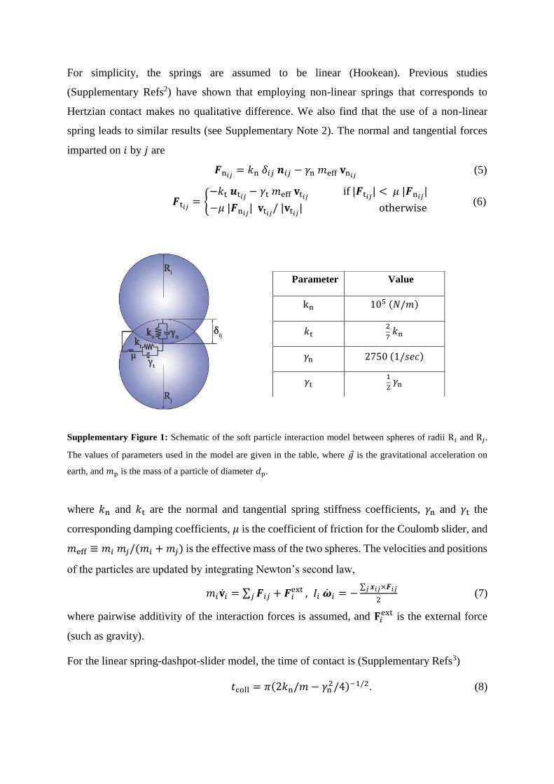
The Discrete Element Method (DEM) is a particle dynamics simulator with an elastoplastic

interaction force, which is widely used for computational simulation of granular statics and

flow (Supplementary Refs1). Our simulations were conducted using the open source molecular

dynamics package LAMMPS (Supplementary Refs2), and the contact model and its DEM

implementation are described in Supplementary Refs3. In DEM the particles are treated as

deformable, and their interaction forces are calculated from the normal overlap and tangential

displacement post contact. The dissipative interaction is modelled by spring-dashpot modules

for the normal and tangential directions (Supplementary Fig. 1), and an additional Coulomb

slider in the latter to incorporate a rate-independent frictional force, an important feature of

granular materials. For a pair of spheres 𝑖, 𝑗 of radii 𝑅𝑖, 𝑅𝑗 at positions 𝒙𝑖, 𝒙𝑗 in contact, the

overlap is

𝛿 ≡ 𝑅𝑖 + 𝑅𝑗 − |𝒙𝑖j| (1)

where 𝒙𝑖𝑗 ≡ 𝒙𝑖 − 𝒙𝑗; the particles are in contact only when the overlap is positive. The

components of the relative velocity normal and tangential to the point of contact are

𝐯n𝑖𝑗= (𝐯𝑖𝑗 . 𝒏𝑖𝑗) 𝒏𝑖𝑗 (2)

𝐯t𝑖𝑗= 𝐯𝑖𝑗 − 𝐯𝑛𝑖𝑗

− (𝝎𝑖𝑅𝑖 + 𝝎𝑗𝑅𝑗)  ×  𝒏𝑖𝑗 (3)

where 𝒏𝑖𝑗 ≡ 𝒙𝑖𝑗/|𝒙𝑖𝑗| is the unit normal from 𝑗 to 𝑖, 𝐯𝑖𝑗 ≡ 𝐯𝑖 − 𝐯𝑗, and 𝝎𝑖, 𝝎𝑗 are the rotational

velocities of particles 𝑖 and 𝑗. The tangential spring displacement 𝒖t𝑖𝑗 is initiated at the time of

contact and can be calculated by integrating,

𝑑𝒖t𝑖𝑗

𝑑𝑡= 𝐯t𝑖𝑗

−(𝒖t𝑖𝑗

.𝐯𝑖𝑗)𝒙𝑖𝑗

|𝒓𝑖𝑗2 |

(4)

The second term represents rigid body rotation around the point of contact and ensures that 𝒖t𝑖𝑗

lies in the tangent plane of contact.

For simplicity, the springs are assumed to be linear (Hookean). Previous studies

(Supplementary Refs2) have shown that employing non-linear springs that corresponds to

Hertzian contact makes no qualitative difference. We also find that the use of a non-linear

spring leads to similar results (see Supplementary Note 2). The normal and tangential forces

imparted on 𝑖 by 𝑗 are

𝑭n𝑖𝑗= 𝑘n 𝛿𝑖𝑗 𝒏𝑖𝑗 − 𝛾n 𝑚eff 𝐯n𝑖𝑗

(5)

𝑭t𝑖𝑗= {

−𝑘t 𝒖t𝑖𝑗− 𝛾t 𝑚eff 𝐯t𝑖𝑗

if |𝑭t𝑖𝑗| < 𝜇 |𝑭n𝑖𝑗

|

−𝜇 |𝑭n𝑖𝑗| 𝐯t𝑖𝑗

/ |𝐯t𝑖𝑗| otherwise

(6)

Parameter Value

kn 105 (𝑁/𝑚)

𝑘t 2

7 𝑘n

𝛾n 2750 (1/𝑠𝑒𝑐)

𝛾t 1

2 𝛾n

Supplementary Figure 1: Schematic of the soft particle interaction model between spheres of radii R𝑖 and R𝑗.

The values of parameters used in the model are given in the table, where 𝑔 is the gravitational acceleration on

earth, and 𝑚p is the mass of a particle of diameter 𝑑p.

where 𝑘n and 𝑘t are the normal and tangential spring stiffness coefficients, 𝛾n and 𝛾t the

corresponding damping coefficients, 𝜇 is the coefficient of friction for the Coulomb slider, and

𝑚eff ≡ 𝑚𝑖 𝑚𝑗/(𝑚𝑖 + 𝑚𝑗) is the effective mass of the two spheres. The velocities and positions

of the particles are updated by integrating Newton’s second law,

𝑚𝑖�̇�𝑖 = ∑ 𝑭𝑖𝑗 + 𝑭𝑖ext

𝑗 , 𝐼𝑖 �̇�𝑖 = −∑ 𝒙𝑖𝑗𝑗 ×𝑭𝑖𝑗

2 (7)

where pairwise additivity of the interaction forces is assumed, and 𝐅𝑖ext is the external force

(such as gravity).

For the linear spring-dashpot-slider model, the time of contact is (Supplementary Refs3)

𝑡coll = 𝜋(2𝑘n/𝑚 − 𝛾n2/4)−1/2. (8)

The choice of the normal spring stiffness coefficient determines the collision time between two

particles. The simulation time step is chosen such that each collision is resolved accurately,

and the choice of ∆𝑡 = 𝑡coll/50 is found to be sufficiently small6 (Supplementary Refs3). Since

the collision time decreases with increasing spring stiffness 𝑘n, it is standard practice to

optimize the value of 𝑘n such that it is large enough for the macroscopic behaviour to mimic

that of hard particles, and the time step is large enough for the computations to be tractable.

The parameters used in the simulations are listed in Supplementary Fig. 1.

The values of 𝑘n, 𝑘t and 𝛾t was chosen based on previous studies6 (Supplementary Refs3) that

have attempted to model hard grains such as glass beads and sand. The value of 𝛾n chosen is

such that the normal coefficient of restitution is 0.7. In all our computations, 𝜇 is set to 0.5. The

2d simulations were conducted by placing spheres in a plane and allowing movement only

within the plane.

In our simulations, the mean particle size is 1cm (𝑑𝑝), and the particle sizes were chosen from

a uniform distribution with lower and upper limits of 0.8𝑑𝑝 and 1.2𝑑p respectively. The walls

were constructed with particles of diameter 𝑑p set in a close packed linear (2d) or triangular

(3d) lattice. In all the simulations, the constants characterizing grain-wall interactions are the

same as those for grain-grain interactions.

Supplementary Note 2

1. Method of deposition

1.1 Piles

1.1.1 Narrow source

(a) Deposition from a vertical narrow region

In the narrow source deposition procedure, non-overlapping particles were randomly created

in a narrow region (coloured grey in Supplementary Fig. 4), and were allowed to fall under the

influence of gravity, 𝑔 . Here, the region of deposition is randomly filled with non-overlapping

particles to a volume fraction of 0.1 (area fraction of 0.2 in 2d), and the next set of particles are

created after the current set has moved out of the deposition region under the influence of

gravity. In 2d, the length and width of the deposition area is, 𝐿𝐷 = 50𝑑𝑝, and, 𝑊𝐷 = 10𝑑𝑝

respectively (see Supplementary Fig. 4a). In 3d, the deposition region was a cylinder with

length, 𝐿𝐷 = 60𝑑𝑝 and radius, 𝑅𝐷 = 7𝑑𝑝. The deposition area was located at a fixed height,

𝐻𝐷 = 60𝑑𝑝 (in 2d) (50𝑑𝑝 in 3d) from the supporting base of the pile. The deposition was

continued till a fixed number of particles were poured and the simulations were continued till

the kinetic energy per particle decreased to a value of 10−12𝐽. The narrow source deposited

piles described in Fig. 2 were created by this procedure. The dimensions of the piles created

are given in Supplementary Table 1. Unless specified otherwise, narrow source deposited piles

described in this study were created by this procedure.

Method of

deposition Height, 𝑯𝑷 Radius, 𝑹𝑷 Angle of repose, 𝝓𝒓

2d, Narrow source 42 144.5 16.20

2d, Narrow source

(1.1.1b) 45 143 17.47

2d, Hopper 41 148 15.48

2d, Rained 42 125 18.57

3d, Narrow source 34 94 19.89

3d, Rained 28 90 17.28

Supplementary Table 1: Dimensions of the piles created by different methods of deposition. In all cases, the

radius of the pile (𝑅𝑝) is the minimum distance from the centre at which the average height of the pile is ≈ 1𝑑𝑝 ±

(𝑑𝑝/4).

(b) Deposition from a vertical narrow region with reduced length and lesser height of

deposition

The effect of height of the deposition region on the central stress minimum in 2d piles deposited

from a narrow source was studied. To reduce the effects of impact force generated by the newly

poured particles, we deposited from a region with 𝐻𝐷 = 45𝑑𝑝, and 𝐿𝑑 × 𝑊𝑑(10𝑑𝑝 × 10𝑑𝑝)

(see Supplementary Fig. 4a), and the fraction of area filled with particles is 0.4. We note that,

the height of the pile (𝐻𝑝 = 42𝑑𝑝) is comparable to the 𝐻𝐷. In addition, the reduced length of

the deposition region (by a factor of 5), considerably reduces the impact force generated due

to the newly poured particles. As given in Supplementary Table 1, the reduced effect of impact

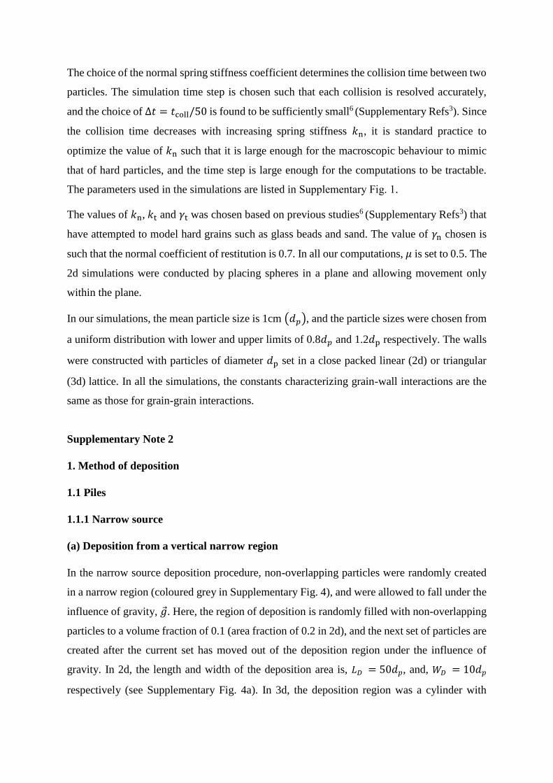
force results in a slightly steeper pile. We find that, the spatial structure patterns and stress

profiles measured at the supporting base are similar to the previous case (see Supplementary

Fig. 2). However, in piles made of stiffer particles (𝑘𝑛 = 106), increasing heights of deposition

affects the shape of the free surface of the pile. Hence, to construct piles with stiffer particles,

we used a lower height of deposition (𝐻𝐷 = 45𝑑𝑝). The dimensions of the piles created are

given in Supplementary Table 1.

(a) (b)

Supplementary Figure 2: Spatial structure of piles created by depositing particles from a vertical narrow region

with reduced length and lesser height of deposition. Dashed lines represent the average height of the free surface

of the pile. (a) Contact lines (black) and force lines (blue). (b) RW predications compared with the estimates

from particle dynamics simulations. σ𝑦𝑦 is the normal stress measured at the supporting base and 𝑇𝑊 is the total

weight of the pile.

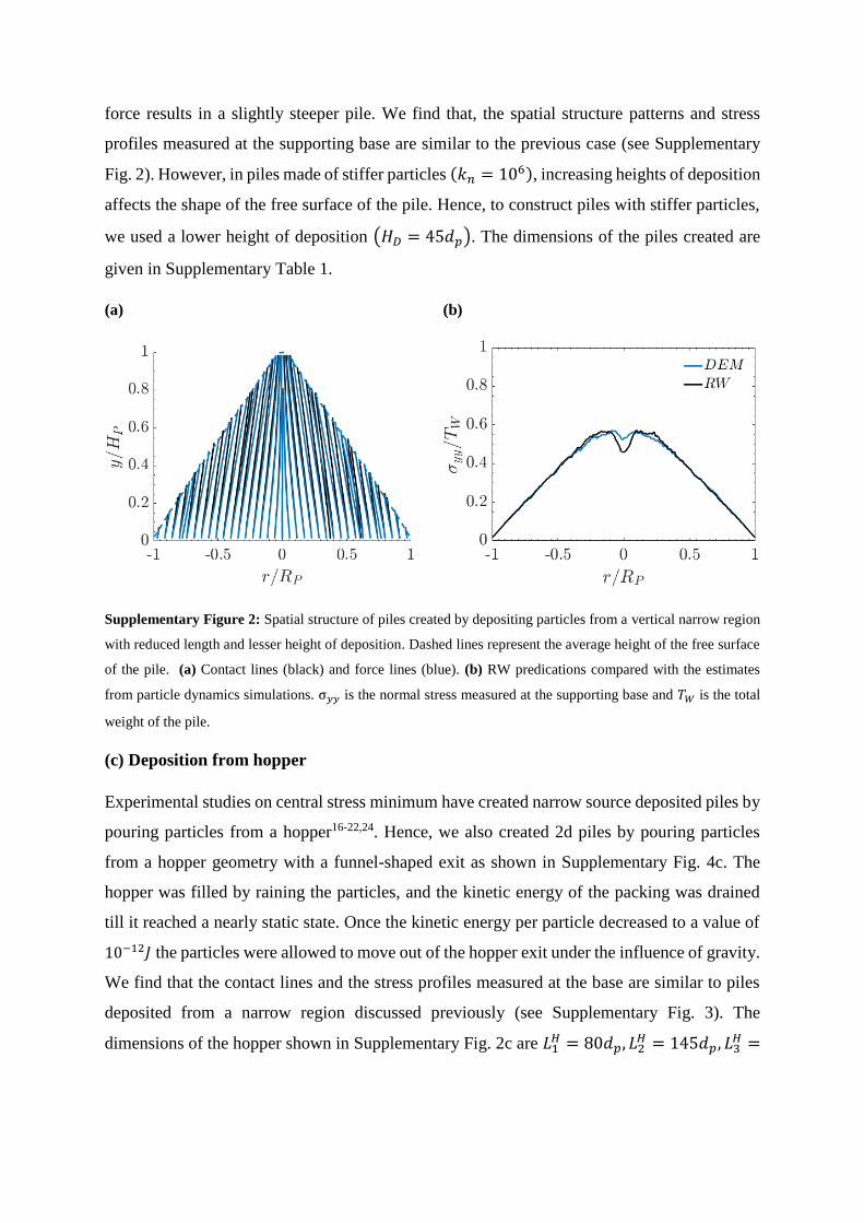
(c) Deposition from hopper

Experimental studies on central stress minimum have created narrow source deposited piles by

pouring particles from a hopper16-22,24. Hence, we also created 2d piles by pouring particles

from a hopper geometry with a funnel-shaped exit as shown in Supplementary Fig. 4c. The

hopper was filled by raining the particles, and the kinetic energy of the packing was drained

till it reached a nearly static state. Once the kinetic energy per particle decreased to a value of

10−12𝐽 the particles were allowed to move out of the hopper exit under the influence of gravity.

We find that the contact lines and the stress profiles measured at the base are similar to piles

deposited from a narrow region discussed previously (see Supplementary Fig. 3). The

dimensions of the hopper shown in Supplementary Fig. 2c are 𝐿1𝐻 = 80𝑑𝑝, 𝐿2

𝐻 = 145𝑑𝑝, 𝐿3𝐻 =

50𝑑𝑝,𝑊𝑑 = 300𝑑𝑝, 𝑅𝑜 = 10𝑐𝑚 and 𝐻𝑑 = 50𝑑𝑝. The dimensions of the piles created are

given in Supplementary Table 1.

(a) (b)

Supplementary Figure 3: Spatial structure of piles created by depositing particles from a hopper. (a) Contact

lines (black) and force lines (blue). Dashed lines represent the average height of the free surface of the pile. (b)

RW predications compared with the estimates from particle dynamics simulations. σ𝑦𝑦 is the normal stress

measured at the supporting base and 𝑇𝑊 is the total weight of the pile.

1.1.2 Rained

In the rained deposition method, the width of the deposition (𝑊𝐷) region was equal to the

radius of the heap, 𝑅𝑃 (see Supplementary Fig. 4b). Other aspects of the deposition procedure

are similar to the narrow source deposition method. In 3d, the deposition region is a cylinder

of length 𝐿𝐷, and radius 𝑅𝐷, with dimensions 10𝑑𝑝 × 90𝑑𝑝 (𝐿𝐷 × 𝑅𝐷). The rained piles

described in Fig. 2 were created by this procedure. The dimensions of the piles created are

given in Supplementary Table 1. Unless specified otherwise, rained piles described in this study

were created by this procedure.

(a)

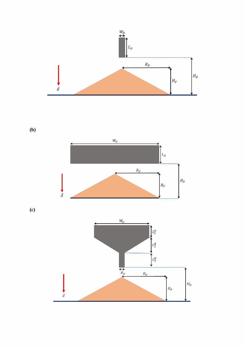
(b)

(c)

Supplementary Figure 4: Schematic of different methods of deposition. (a) Narrow source deposition (b)

deposition by raining (c) deposition from a hopper. In all cases, the region of deposition in shown in grey.

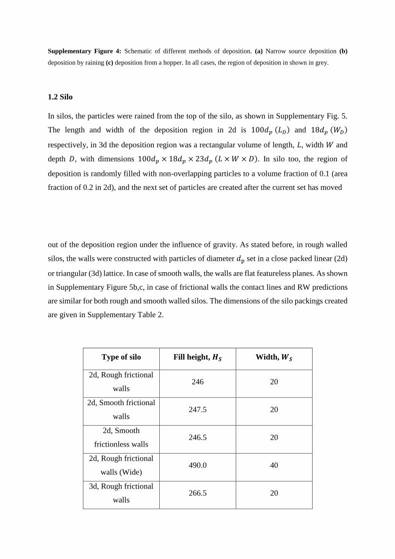
1.2 Silo

In silos, the particles were rained from the top of the silo, as shown in Supplementary Fig. 5.

The length and width of the deposition region in 2d is 100𝑑𝑝 (𝐿𝐷) and 18𝑑𝑝 (𝑊𝐷)

respectively, in 3d the deposition region was a rectangular volume of length, 𝐿, width 𝑊 and

depth 𝐷, with dimensions 100𝑑𝑝 × 18𝑑𝑝 × 23𝑑𝑝 (𝐿 × 𝑊 × 𝐷). In silo too, the region of

deposition is randomly filled with non-overlapping particles to a volume fraction of 0.1 (area

fraction of 0.2 in 2d), and the next set of particles are created after the current set has moved

out of the deposition region under the influence of gravity. As stated before, in rough walled

silos, the walls were constructed with particles of diameter 𝑑p set in a close packed linear (2d)

or triangular (3d) lattice. In case of smooth walls, the walls are flat featureless planes. As shown

in Supplementary Figure 5b,c, in case of frictional walls the contact lines and RW predictions

are similar for both rough and smooth walled silos. The dimensions of the silo packings created

are given in Supplementary Table 2.

Type of silo Fill height, 𝑯𝑺 Width, 𝑾𝑺

2d, Rough frictional

walls 246 20

2d, Smooth frictional

walls 247.5 20

2d, Smooth

frictionless walls 246.5 20

2d, Rough frictional

walls (Wide) 490.0 40

3d, Rough frictional

walls 266.5 20

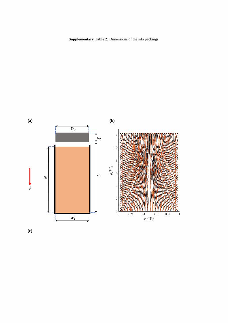
Supplementary Table 2: Dimensions of the silo packings.

(a) (b)

(c)

Supplementary Figure 5: Schematic and contact lines of a silos (a) Schematic of a silo packing, with the region

of deposition shown in grey. (b) Comparison of contact lines in 2d silos with rough frictional walls (black) and

smooth frictional walls (brown). (c) Predications of RW compared to the estimate from particle dynamics

simulations in 2d silos with smooth frictional walls. 𝐹 is the average contact force at a given depth from the free

surface of the silo (𝐹𝑛 in DEM, and 𝐹𝑅𝑊 in RW (see Methods section for details)), 𝑇𝑊 is the total weight of the

system.

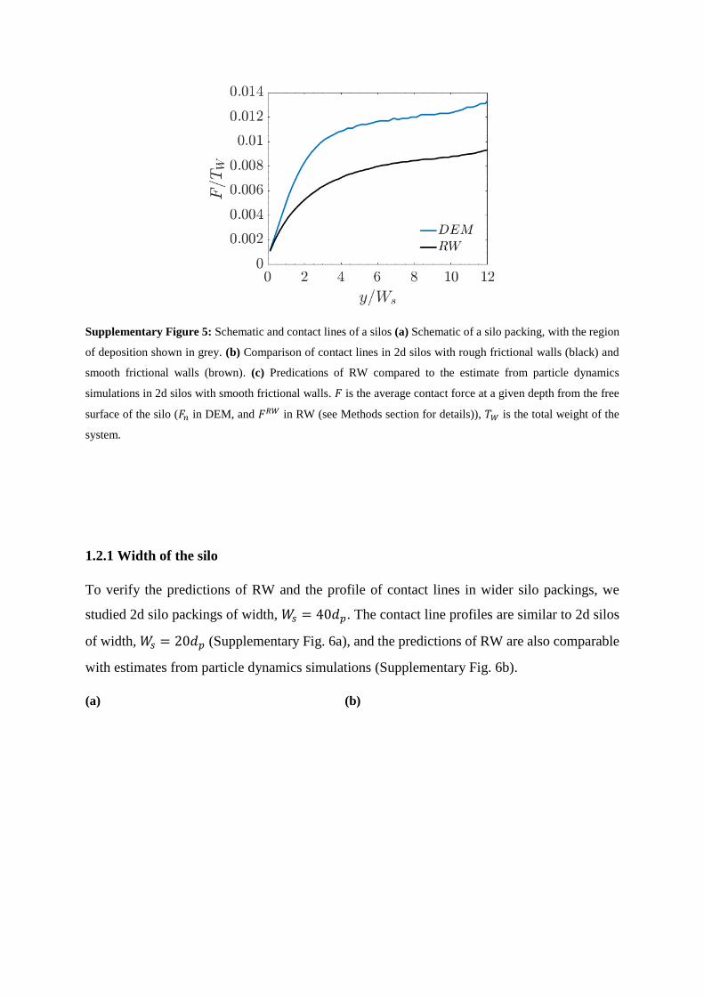
1.2.1 Width of the silo

To verify the predictions of RW and the profile of contact lines in wider silo packings, we

studied 2d silo packings of width, 𝑊𝑠 = 40𝑑𝑝. The contact line profiles are similar to 2d silos

of width, 𝑊𝑠 = 20𝑑𝑝 (Supplementary Fig. 6a), and the predictions of RW are also comparable

with estimates from particle dynamics simulations (Supplementary Fig. 6b).

(a) (b)

Supplementary Figure 6: Spatial structure of 2d silos with different widths (𝑊𝑠), the aspect ratio (𝐻𝑠/𝑊𝑠) is ≈

12 in both cases. (a) Comparison of contact lines (𝑊𝑠 = 20𝑑𝑝, black) (𝑊𝑠 = 40𝑑𝑝, brown). (b) The predications

of RW in the larger silo (𝑊𝑠 = 40𝑑𝑝) compared to the estimates from particle dynamics simulations. 𝐹 is the

average contact force at a given depth from the free surface of the silo (𝐹𝑛 in DEM, and 𝐹𝑅𝑊 in RW (see Methods

section for details)), 𝑇𝑊 is the total weight of the system.

2. Contact model

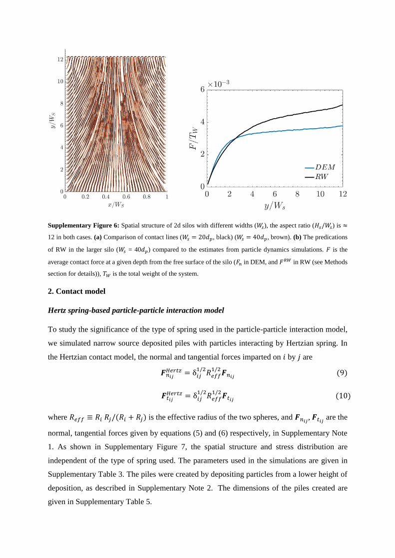
Hertz spring-based particle-particle interaction model

To study the significance of the type of spring used in the particle-particle interaction model,

we simulated narrow source deposited piles with particles interacting by Hertzian spring. In

the Hertzian contact model, the normal and tangential forces imparted on 𝑖 by 𝑗 are

𝑭𝑛𝑖𝑗

𝐻𝑒𝑟𝑡𝑧 = δ𝑖𝑗1/2

𝑅𝑒𝑓𝑓1/2

𝑭𝑛𝑖𝑗 (9)

𝑭𝑡𝑖𝑗𝐻𝑒𝑟𝑡𝑧 = δ𝑖𝑗

1/2𝑅𝑒𝑓𝑓

1/2𝑭𝑡𝑖𝑗

(10)

where 𝑅𝑒𝑓𝑓 ≡ 𝑅𝑖 𝑅𝑗/(𝑅𝑖 + 𝑅𝑗) is the effective radius of the two spheres, and 𝑭𝑛𝑖𝑗, 𝑭𝑡𝑖𝑗

are the

normal, tangential forces given by equations (5) and (6) respectively, in Supplementary Note

1. As shown in Supplementary Figure 7, the spatial structure and stress distribution are

independent of the type of spring used. The parameters used in the simulations are given in

Supplementary Table 3. The piles were created by depositing particles from a lower height of

deposition, as described in Supplementary Note 2. The dimensions of the piles created are

given in Supplementary Table 5.

(a) (b)

Supplementary Figure 7: Spatial structure of piles created by depositing particles interacting with a Hertzian

spring in the contact model. Dashed lines represent the average height of the free surface of the pile. (a) Contact

lines (black) and force lines (blue). (b) RW predications compared with the estimates from particle dynamics

simulations. σ𝑦𝑦 is the normal stress measured at the supporting base and 𝑇𝑊 is the total weight of the pile.

Parameter Value

𝑘n(𝑁/𝑚) 106

𝑘t(𝑁/𝑚) 2

7 𝑘n

𝛾n(1/𝑠𝑒𝑐) 8698

𝛾t(1/𝑠𝑒𝑐) 1

2 𝛾n

Supplementary Table 3: Parameters used in the Hertz spring-based contact model.

3. Interaction parameters in the linear spring and dashpot model

In this section, we describe the effect of various parameters in the linear spring and dashpot

model used in this study.

3.1 Spring stiffness

The contact line patterns, and the base stress distribution do not show a considerable difference

with varying spring stiffness of the particles (see Supplementary Figure 8). Interestingly with

increase in the spring stiffness coefficient of the particles, we find that the predictions of the

random walk agree well with the DEM results. This further shows that, the random walk is a

reasonable model of force transmission in granular piles, as particles with large spring stiffness

values correspond well with realistic granular materials. We note that, the piles made of

particles with 𝑘𝑛 = 106 shown in Supplementary Figure 8 were created by depositing particles

from a lower height of deposition (see Supplementary Note 2). Here, the value of 𝛾n chosen is

such that the normal coefficient of restitution is 0.7. Other interaction parameters are as

described in Supplementary Table 4, and 𝜇 = 0.5. The dimensions of the piles created are given

in Supplementary Table 5.

(a) (b)

(c) (d)

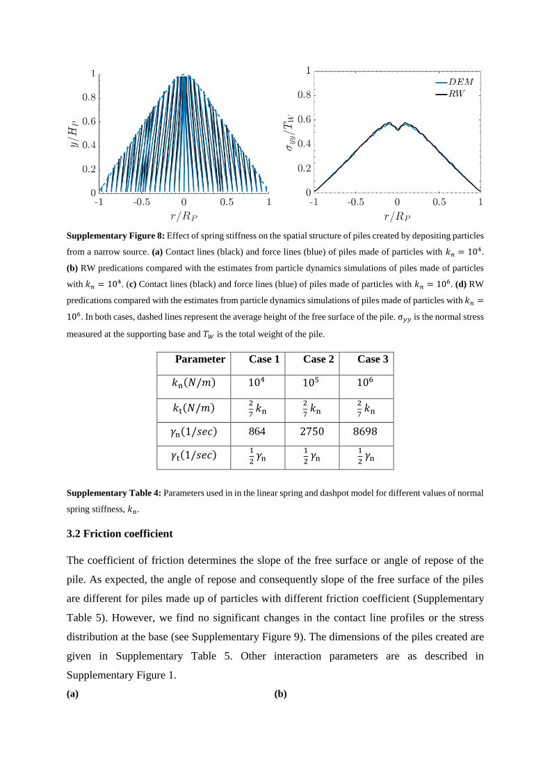
Supplementary Figure 8: Effect of spring stiffness on the spatial structure of piles created by depositing particles

from a narrow source. (a) Contact lines (black) and force lines (blue) of piles made of particles with 𝑘𝑛 = 104.

(b) RW predications compared with the estimates from particle dynamics simulations of piles made of particles

with 𝑘𝑛 = 104. (c) Contact lines (black) and force lines (blue) of piles made of particles with 𝑘𝑛 = 106. (d) RW

predications compared with the estimates from particle dynamics simulations of piles made of particles with 𝑘𝑛 =

106. In both cases, dashed lines represent the average height of the free surface of the pile. σ𝑦𝑦 is the normal stress

measured at the supporting base and 𝑇𝑊 is the total weight of the pile.

Parameter Case 1 Case 2 Case 3

𝑘n(𝑁/𝑚) 104 105 106

𝑘t(𝑁/𝑚) 2

7 𝑘n

2

7 𝑘n

2

7 𝑘n

𝛾n(1/𝑠𝑒𝑐) 864 2750 8698

𝛾t(1/𝑠𝑒𝑐) 1

2 𝛾n

1

2 𝛾n

1

2 𝛾n

Supplementary Table 4: Parameters used in in the linear spring and dashpot model for different values of normal

spring stiffness, 𝑘n.

3.2 Friction coefficient

The coefficient of friction determines the slope of the free surface or angle of repose of the

pile. As expected, the angle of repose and consequently slope of the free surface of the piles

are different for piles made up of particles with different friction coefficient (Supplementary

Table 5). However, we find no significant changes in the contact line profiles or the stress

distribution at the base (see Supplementary Figure 9). The dimensions of the piles created are

given in Supplementary Table 5. Other interaction parameters are as described in

Supplementary Figure 1.

(a) (b)

(c) (d)

Supplementary Figure 9: Effect of friction coefficient on the spatial structure of piles created by depositing

particles from a narrow source. (a) Contact lines (black) and force lines (blue) of piles made of particles with 𝜇 =

0.25. (b) RW predications compared with the estimates from particle dynamics simulations of piles made of

particles with 𝜇 = 0.25. (c) Contact lines (black) and force lines (blue) of piles made of particles with 𝜇 = 0.75.

(d) RW predications compared with the estimates from particle dynamics simulations of piles made of particles

with 𝜇 = 0.75. In both cases, dashed lines represent the average height of the free surface of the pile. σ𝑦𝑦 is the

normal stress measured at the supporting base and 𝑇𝑊 is the total weight of the pile.

3.3 Size distribution of the particles

A key finding of our study is the importance of particle size distribution on the spatial structure

of the pile. A complete understanding of the effect of polydispersity in granular piles requires

a detailed study on the type of distribution and the range of polydispersity. Hence, we studied

piles made of particles with a narrow distribution of particle sizes compared to the range of

polydispersity of 20% used in all polydisperse cases in this study. Here, δ = 10%, and the

particle sizes were uniformly distributed. As shown in Supplementary Figure 10, we find that

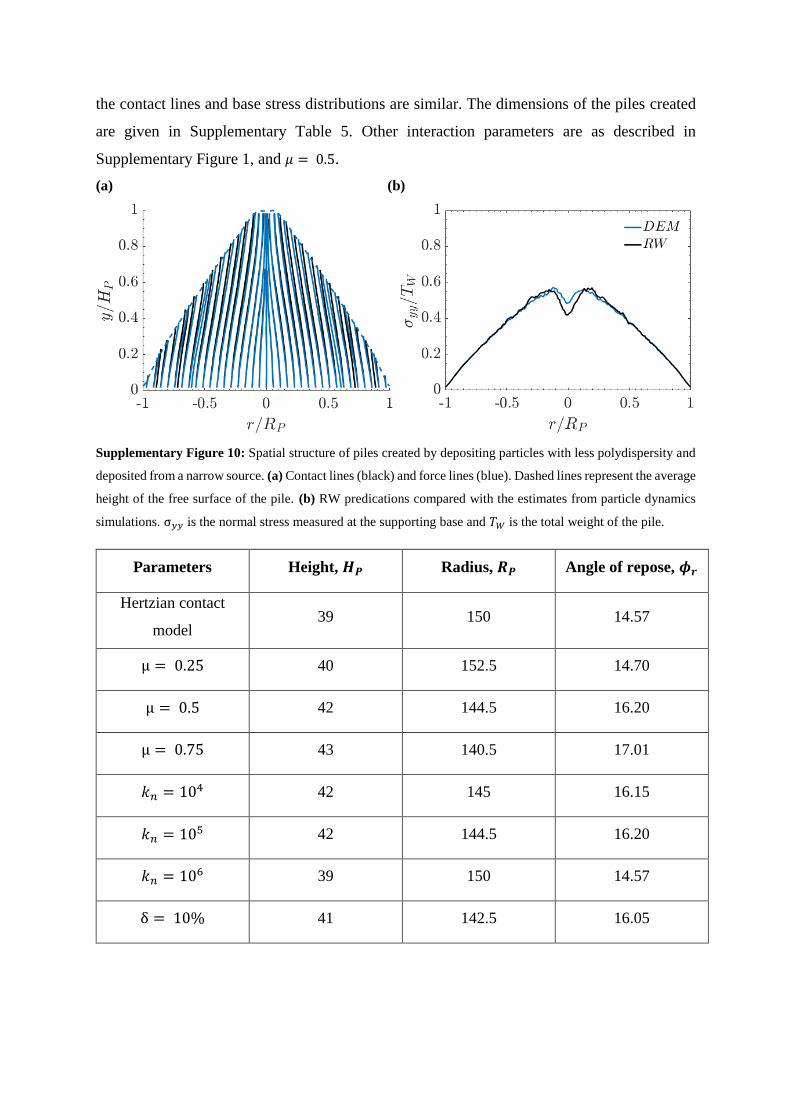
the contact lines and base stress distributions are similar. The dimensions of the piles created

are given in Supplementary Table 5. Other interaction parameters are as described in

Supplementary Figure 1, and 𝜇 = 0.5.

(a) (b)

Supplementary Figure 10: Spatial structure of piles created by depositing particles with less polydispersity and

deposited from a narrow source. (a) Contact lines (black) and force lines (blue). Dashed lines represent the average

height of the free surface of the pile. (b) RW predications compared with the estimates from particle dynamics

simulations. σ𝑦𝑦 is the normal stress measured at the supporting base and 𝑇𝑊 is the total weight of the pile.

Parameters Height, 𝑯𝑷 Radius, 𝑹𝑷 Angle of repose, 𝝓𝒓

Hertzian contact

model 39 150 14.57

μ = 0.25 40 152.5 14.70

μ = 0.5 42 144.5 16.20

μ = 0.75 43 140.5 17.01

𝑘𝑛 = 104 42 145 16.15

𝑘𝑛 = 105 42 144.5 16.20

𝑘𝑛 = 106 39 150 14.57

δ = 10% 41 142.5 16.05

Supplementary Table 5: Dimensions of 2d piles deposited from a narrow source for different values of

parameters in the linear spring and dashpot model. In all cases, the radius of the pile (𝑅𝑝) is the minimum distance

from the centre at which the average height of the pile is ≈ 1𝑑𝑝 ± (𝑑𝑝/4).

4. Averaging procedure and number of independent configurations studied

4.1 Base stress profiles in piles

(a) 2d piles

The base stress profiles in all cases of 2d piles were obtained by running averages with a

window length of 7𝑑𝑝, we found that 7𝑑𝑝 is necessary for obtaining reasonably smooth

averages of base stress profiles. Hence, for every base particle of diameter 𝑑𝑝 at a horizontal

coordinate 𝑥𝑝, the base stress values are averaged in the range [𝑥𝑝– 3𝑑𝑝, 𝑥𝑝 + 3𝑑𝑝]. The

number of configurations used in obtaining the results reported for 2d piles is 400 for all cases,

except for results reported in Fig. 2-4, where 1000 configurations were used.

(b) 3d piles

The base stress profiles in 3d piles were obtained by averaging in radial rings of width, ∆𝑟 =

𝑟𝑜– 𝑟𝑖 = 3𝑑𝑝, where 𝑟𝑖 is the inner radius and 𝑟𝑜 is the outer radius of the ring. The number of

configurations used in obtaining the results reported for 3d piles is 30 for all cases.

(c) 2d and 3d silos

The normal contact force in all cases of 2d and 3d silo packings were averaged in vertical bins

of height, ∆ℎ = 5𝑑𝑝. The number of configurations used in obtaining the results reported for

2d and 3d silo packings is 600 and 300 respectively for all cases.

Supplementary Note 3

Comparison of the contact lines, force lines and random walk lines in pile and silo

packings

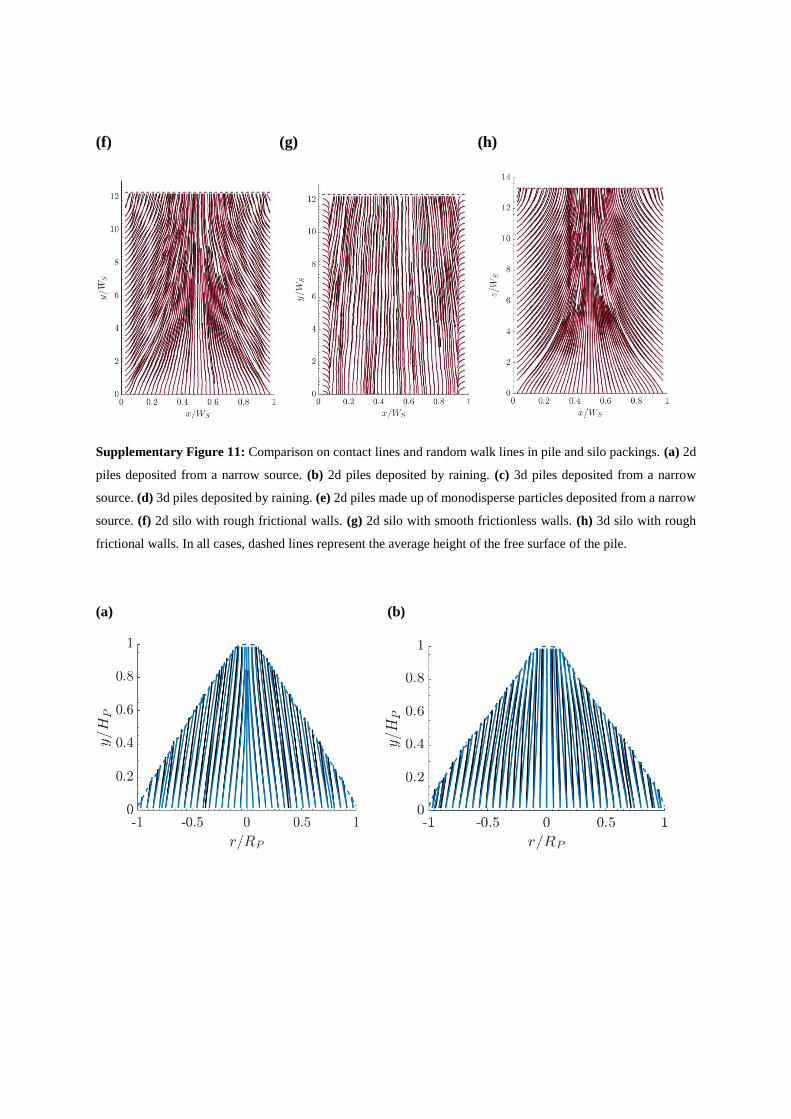
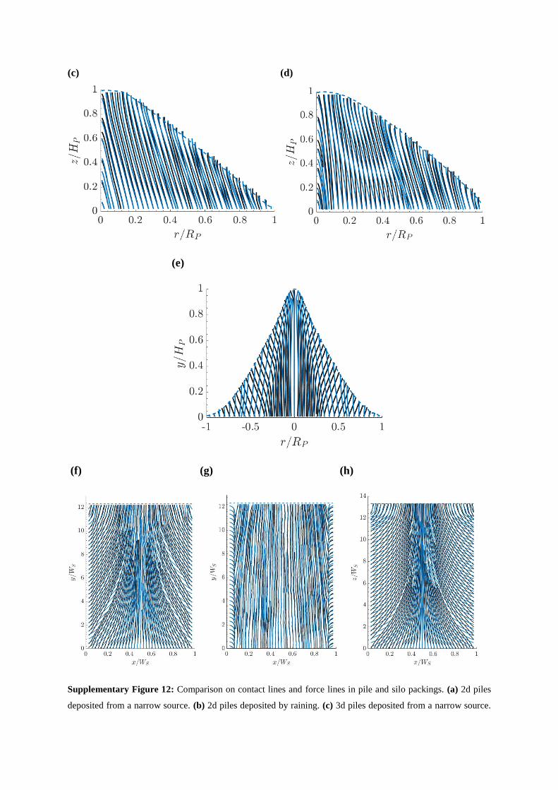
In all types of packings considered in this study, we find that the contact lines and random walk

lines are almost similar (see Supplementary Figure 11). In granular piles, we find that the force

lines too agree well with contact lines and random walk lines, except monodisperse case (see

Supplementary Figure 12a-e). In silos, the force lines show strong curvature towards the lateral

walls compared to the contact lines (see Supplementary Figure 12f-h).

(a) (b)

(c) (d)

(e)

(f) (g) (h)

Supplementary Figure 11: Comparison on contact lines and random walk lines in pile and silo packings. (a) 2d

piles deposited from a narrow source. (b) 2d piles deposited by raining. (c) 3d piles deposited from a narrow

source. (d) 3d piles deposited by raining. (e) 2d piles made up of monodisperse particles deposited from a narrow

source. (f) 2d silo with rough frictional walls. (g) 2d silo with smooth frictionless walls. (h) 3d silo with rough

frictional walls. In all cases, dashed lines represent the average height of the free surface of the pile.

(a) (b)

(c) (d)

(e)

(f) (g) (h)

Supplementary Figure 12: Comparison on contact lines and force lines in pile and silo packings. (a) 2d piles

deposited from a narrow source. (b) 2d piles deposited by raining. (c) 3d piles deposited from a narrow source.

(d) 3d piles deposited by raining. (e) 2d piles made up of monodisperse particles deposited from a narrow source.

(f) 2d silo with rough frictional walls. (g) 2d silo with smooth frictionless walls. (h) 3d silo with rough frictional

walls. In all cases, dashed lines represent the average height of the free surface of the pile.

Supplementary Note 4

Details of supplementary videos

In all the following supplementary videos, for polydisperse packings, the particle sizes were

chosen from a uniform distribution with lower and upper limits of 0.8𝑑𝑝 and 1.2𝑑𝑝

respectively, where 𝑑𝑝 is the mean diameter. We refer to the displacement vector field as 𝑆 ,

and is defined as 𝑟�⃗⃗�  – 𝑟𝑖⃗⃗ , where 𝑟𝑖⃗⃗ is the position vector of the particle at time 𝑡𝑖. We have chosen

the ∆𝑡𝑖𝑗 = 𝑡𝑗– 𝑡𝑖 as 1\4 𝑠𝑒𝑐, we found this time interval sufficient for obtaining a smooth

visualisation of time evolution of both 𝑆 and �⃗� vector fields, and in all cases of pile and silo

packings.

And, all the properties (𝑆 , �⃗� ) were averaged in a 1 × 1 (𝑑𝑝 × 𝑑𝑝) spatial grid, which was

further averaged over 300 independent realizations. Note, here unlike �⃗� , 𝑆 in all directions are

considered for obtaining the averages. Also, the time of the video does not correspond to the

simulation time and is given below. The video shows the time evolution of all cases till |𝑆 |

decreases to less than 0.01𝑑𝑝 in every spatial grid.

Supplementary videos 1-5 (time evolution of contact lines)

Evolution of contact lines in 2d pile and silo packings. The lines indicate the streamlines of the

spatially averaged �⃗� vector field. The background colour shows the contour maps based on the

particle IDs. The particles IDs are assigned based on the time of deposition scaled by the

maximum particle ID (the ID of the last deposited particle).

1. Supplementary video 1 – Evolution of contact lines in polydisperse piles deposited

from a narrow source. The simulation time of the video is 42 seconds.

2. Supplementary video 2 – Evolution of contact lines in polydisperse piles created by

raining the particles. The simulation time of the video is 16 seconds.

3. Supplementary video 3 – Evolution of contact lines in monodisperse piles deposited

from a narrow source. The simulation time of the video is 47 seconds.

4. Supplementary video 4 – Evolution of contact lines in polydisperse silo packings

created by raining the particles into a container with frictional walls. The simulation

time of the video is 18 seconds.

5. Supplementary video 5 – Evolution of contact lines in polydisperse silo packings

created by raining the particles into a container with smooth frictionless walls. The

simulation time of the video is 46 seconds.

Supplementary videos 6-10 (time evolution of displacement field of particles)

Evolution of streamlines based on the displacement field (𝑆 ) of particles in 2d pile and silo

packings. The lines indicate the streamlines of the spatially averaged displacement field, 𝑆 , and

the background colour shows the contour map of |𝑆 | scaled by 𝑑𝑝 in logarithmic scale (𝑙𝑜𝑔10).

Note that for clarity, the streamlines are shown only if |𝑆 | ≥ 0.01𝑑𝑝, And, the maximum and

minimum value of the background colour is set as 100𝑑𝑝 and 0.01𝑑𝑝 respectively. If |𝑆 | is

greater than 100𝑑𝑝 then it is set to 100𝑑𝑝, and similarly, if |𝑆 | less than 0.01𝑑𝑝 then it is set

to 0.01𝑑𝑝.

1. Supplementary video 6 – Evolution of streamlines based on 𝑆 in polydisperse piles

deposited from a narrow source. The simulation time of the video is 42 seconds.

2. Supplementary video 7 – Evolution of streamlines based on 𝑆 in polydisperse piles

created by raining the particles. The simulation time of the video is 16 seconds.

3. Supplementary video 8 – Evolution of streamlines based on 𝑆 in monodisperse piles

deposited from a narrow source. The simulation time of the video is 47 seconds.

4. Supplementary video 9 – Evolution of streamlines based on 𝑆 in polydisperse silo

packings created by raining the particles into a container with frictional walls. The

simulation time of the video is 18 seconds. In frictional silos, a perceptible flow is

observed only in the growing free surface region. Hence, we shift the vertical axis

accordingly in time to clearly show the flow in the growing free surface region.

5. Supplementary video 10 – Evolution of streamlines based on 𝑆 in polydisperse silo

packings created by raining the particles into a container with smooth frictionless walls.

The simulation time of the video is 46 seconds.

Supplementary References

1. Cundall, P. A., & Strack, O. D. A discrete numerical model for granular

assemblies. Geotechnique 29, 47-65 (1979).

2. Plimpton, S. Fast parallel algorithms for short-range molecular dynamics. J. Comput.

Phys. 117, 1-19 (1995).

3. Silbert, L. E., Ertaş, D., Grest, G. S., Halsey, T. C., Levine, D., & Plimpton, S. J.

Granular flow down an inclined plane: Bagnold scaling and rheology. Phys. Rev. E 64,

051302 (2001).