spatial statistical modelling for assessing landslide … · 2011. 6. 23. · goswami, ms. richa...

SPATIAL STATISTICAL MODELLING FOR ASSESSING LANDSLIDE HAZARD AND

VULNERABILITY

Iswar Chandra Das

Examining committee Prof.dr. V.G. Jetten University of Twente Prof.dr. A. Bagchi University of Twente Prof.dr.ir. A.K. Bregt Wageningen University Prof.dr. P.K. Champati Ray IIRS, India Dr. D. Karssenberg Utrecht University Prof.dr. F.D. van der Meer University of Twente ITC dissertation number 192 ITC, P.O. Box 217, 7500 AE Enschede, The Netherlands ISBN 978-90-6164-312-8 Cover designed by Benno Masselink / Job Duim Printed by ITC Printing Department Copyright © 2011 by Iswar Chandra Das This thesis was the outcome of the joint research collaboration between • Indian Institute of Remote Sensing, NRSC, ISRO, India. • Faculty of Geo-information Science and Earth Observation (ITC),

University of Twenty, The Netherlands.

SPATIAL STATISTICAL MODELLING FOR ASSESSING LANDSLIDE HAZARD AND

VULNERABILITY

DISSERTATION

to obtain the degree of doctor at the University of Twente,

on the authority of the Rector Magnificus, prof. dr. H. Brinksma,

on account of the decision of the graduation committee, to be publicly defended

on Tuesday 5 July 2011 at 15:30 hrs

by

Iswar Chandra Das born on 15 June 1969

in Jajpur, India

This thesis is approved by Prof. dr. Alfred Stein, Promoter Dr. Norman Kerle, Assistant promoter

To my late father and mother who brought me to this beautiful world

i

Acknowledgements This thesis could not have been completed without the great support and the encouragement of a number of people. Since at this moment it is difficult to memorize all of them, I would like to apologize for any person I forget to mention. My first and foremost gratitude is expressed to my guide and promoter, Prof Alfred Stein, the one person who kept my confidence and spirit high throughout the research work. Every mail from Prof Stein, whether of appreciation or criticism has contributed to do justice to the thesis in one aspect or other. His professional yet friendly and humorous ways of communication has helped in the successful completion of the thesis with ease and comfort. He encouraged me to think for myself and gave me complete freedom to develop the research, but ensured that the research moved forward and not in circles. I must have sorely tried his patience by long periods of inactivity due to my job commitments; nevertheless, his unbridled support was forthcoming during the entire tenure of my research. I extend my sincere gratitude to Dr. V. K. Dadhwal, Director, NRSC, ISRO, who had nominated me for this joint IIRS-ITC research and kept faith on my abilities for this entire PhD period. Initially, I was interested to carry out PhD on a topic related to hyperspectral remote sensing as I completed my master’s thesis on this subject. However, the encouragement and support I received from Dr. Dadhwal to carry out this research work made me strong to reach at this position finally. Without him, this research work would not have been possible. As a person I found him very calm and considerate. I sincerely thank Dr. Norman Kerle, my co-supervisor, who is really very critical to my work, but at the same time helped me steer through with much dexterity. I have made him unhappy on many occasions due to relatively less communication. But the positive point about him is that he tries to bring out the weakness in a manuscript very accurately, which helped me shape my work in proper direction. I owe him apology, for communicating less with him. I am grateful to Prof. Dr. Victor Jetten and Dr. Cees van Westen for guiding me through out of my research at ITC. They are always present to help me out during my difficult time. Because of my involvement in IIRS-ITC JEP education programme I consider them more as my friend than mentor. A word of gratitude is expressed to Dr. Robert Hack for his guidance during the great field work with him and my student to Himalaya to study the new approach of rock mass classification system for my research work.

ii

I sincerely express my gratitude to Dr. K. Radhakrishnan, Chairman ISRO and Secretary, DOS, for permitting me to do this research in the capacity of Director, NRSC. I am also thankful to Dr. V. Jayaraman, Director NRSC for his kind support and help. I sincerely express my gratitude and thanks to our Dean Dr. P.S. Roy for his kind help and suggestions at the crucial juncture of my PhD. Though brief, but his whole hearted support for my PhD made me feel happy and energetic. A special thank to you sir. I cannot forget to mention Dr. P. K. Champatiray, Head, Geo-sciences Division, IIRS, for the help he has extended in the end of the research. My special thanks to my colleagues and friends Dr. S.K. Srivastav, Dr. Rajat chatterjee, Dr. Ajanta Goswami, Ms. Richa upadhyay, Dr. Yogesh Kant, Mr. Praveen Thakur, Mr. PLN Raju, Dr. Sameer Saran, Mr. Kapil Oberoi, Ms. Vandita Srivastav & Mr. Om Prakash for their help throughout this period of research. Without mentioning all the names I would like to express my thankfulness to all colleagues in IIRS. My special thanks are due to Prof. R. C. Lakhera and late Prof. V. K. Jha. I would also thank to all my Indian friends (not only friends but also like friends & brothers) – Tapas, Saibal, Pankaj, Shekar and many more, who made Holland my second home, when I was here without my family. Special thanks from my inner heart to my IIRS students Sashikant Sahoo, Gaurav Kumar, Jagannath Nayak, Subha Ranjan Mohanty, Pardeep Verma and Ashish Dhiman for their help and support in this special journey. I gratefully acknowledge the academic and technical support I received from Dr Valentijn Tolpekin, ITC. Thank you very much for all your help. I would also like to express my sincere thanks to all staff members of GFM departments, Student Affairs and all technical departments for their kind support. Rishi, Yaseen, Dong Po my very close officemates – thank you friends for your patience, friendly attitude. It was a great pleasure to have friends in and outside PhD community. ITC friends – thank you for your friendship and help. I thank Dr. Takashi Oguchi, Dr. Oliver Korup, Dr. Sunil De, Prof. G. B. Wiersma and several anonymous referees, who reviewed and accepted for publication the papers that I submitted to various journals and offered insightful comments for improving them. Back home, I would like to express my sincere thanks to my wife Tina and my daughter Poonam for their inspiration, moral support and love which enabled me to complete this work. During my stay at Holland for PhD work, I

iii

only know how both (my wife & daughter) had managed alone in Dehradun without me. Still they encouraged me keep working even in the worst condition. Without them this could not have been possible.

“Love you Tina & Poonam.”

Iswar Chandra Das

v

Table of Contents 1. General introduction ...................................................................... 1

1.1 Spatial statistics ........................................................................ 2 1.2 Data and image mining .............................................................. 3 1.3 Landslides and their causes of occurrence ..................................... 4 1.4 Landslide modelling in the context of spatial statistics and data

mining ..................................................................................... 5 1.4.1 Landslide hazard ......................................................... 5 1.4.2 Vulnerability due to landslide .......................................... 8

1.5 Research objectives ................................................................. 10 1.6 Outline of the Thesis ................................................................ 11

2. Comparison between statistical method and field based method for landslide susceptibility assessment ........................... 13

Abstract ......................................................................................... 14 2.1 Introduction ........................................................................... 15 2.2 Research methods and models .................................................. 16

2.2.1 Logistic regression method ............................................ 16 2.2.2 SSPC method ............................................................ 18

2.3 Database preparation ............................................................... 19 2.3.1 Spatial database for the logistic regression analysis .............. 19 2.3.2. Parameterization for the SSPC system .............................. 22

2.4 Results .................................................................................. 31 2.4.1 Logistic regression ...................................................... 31 2.4.2 SSPC method ............................................................ 34

2.5. Comparative analysis and discussion ......................................... 37 2.6. Conclusions ............................................................................ 39

3. Implementation of Strauss point process model for landslide characterization ........................................................................... 41

Abstract ......................................................................................... 42 3.1 Introduction ........................................................................... 43 3.2 Method .................................................................................. 45

3.2.1 Nearest neighbour G-function......................................... 47 3.2.2 Strauss process for marked point pattern .......................... 48 3.2.3 Goodness of fit ........................................................... 48

3.3 Site characteristics and data description ..................................... 49 3.3.1 Data description ......................................................... 50 3.4.1 Model fitting .............................................................. 55

3.5 Discussion .............................................................................. 60 3.6 Conclusions ............................................................................ 62

4. Landslide susceptibility mapping using Bayesian logistic regression models ....................................................................... 63

Abstract ......................................................................................... 64

vi

4.1 Introduction ........................................................................... 65 4.2 Research Methods and Model .................................................... 66 4.3 Site characteristics and database ............................................... 68

4.3.1 Landslide identification and mapping ................................ 69 4.3.2 Landslide influencing factors .......................................... 73

4.4 Implementation ...................................................................... 79 4.5 Results and discussion ............................................................. 81

4.5.1 Landslide spatial probability (susceptibility) map ................. 84 4.5.2 Model validation and accuracy assessment ......................... 85

4.6 Conclusions ............................................................................ 87 5. Landslide hazard assessment using homogeneous susceptible

units (HSU) .................................................................................. 89 Abstract ......................................................................................... 90 5.1 Introduction ........................................................................... 91 5.2 Methods ................................................................................. 93

5.2.1 Spatial probability (susceptibility) modelling and generation of HSU ............................................................. 93

5.2.2 Temporal probability of landslides ........................................ 96 5.2.3 Size probability of landslides ............................................... 97

5.3 Study area and landslide characterization ................................... 98 5.3.1 Site characteristics ............................................................ 98 5.3.2 Landslide identification and mapping .................................. 101

5.4 Hazard assessment ................................................................ 102 5.4.1 Landslide susceptibility assessment ................................... 102 5.4.2 Generation of HSU ......................................................... 104 5.4.3 Temporal probability of landslides ...................................... 106 5.4.4 Probability of landslide size (area) ..................................... 107 5.4.5 Hazard assessment ......................................................... 109

5.5 Discussion and conclusions ..................................................... 110 6. Stochastic landslide vulnerability modelling .............................. 115

Abstract ....................................................................................... 116 6.1 Introduction ......................................................................... 117 6.2 Methods ............................................................................... 119

6.2.1 A probabilistic approach to landslide vulnerability ................ 119 6.2.2 Vulnerability assessment .................................................. 122

6.3 Site characteristics and data collection ..................................... 124 6.3.1 Primary data .................................................................. 126 6.3.2 Secondary data .............................................................. 127

6.4 Results ................................................................................ 128 6.4.1 Vulnerability assessment of buildings ................................. 129 6.4.2 Vulnerability assessment of population in buildings .............. 130 6.4.3 Vulnerability assessment of vehicles on road ....................... 131

6.5 Discussion ............................................................................ 133 6.6 Conclusions .......................................................................... 135

vii

7. Discussions and conclusions ...................................................... 137 7.1 General discussions ............................................................... 138 7.2 Research findings .................................................................. 140

7.2.1 Related to objective 1 ...................................................... 141 7.2.2 Related to objective 2 ...................................................... 141 7.2.3 Related to objective 3 ...................................................... 142 7.2.4 Related to objective 4 ...................................................... 143 7.2.5 Related to objective 5 ...................................................... 144

7.3 Reflections ........................................................................... 145 7.4 Limitations ........................................................................... 146 7.5 Recommendations for further research ..................................... 148

Bibliography ................................................................................... 151 Summary ........................................................................................ 163 Samenvatting ................................................................................. 167 Author’s biography......................................................................... 169 Author’s publications ..................................................................... 170

viii

List of Figures 1.1 Dynamic vulnerability scenario generated due to the time of

occurrence of landslides.............................................................. 10 2.1 Flowchart showing the three step concept of exposure rock mass

(ERM), reference rock mass (RRM) and slope rock mass (SRM), which works in the SSPC system. Modified from Hack et al. (2003) ... 20

2.2 Study area and landslide occurrence map. (A) Ground photo of a landslide. (B) Landslide as depicted on a Cartosat-1 satellite image (scale 1:10,000). (C) Landslide bodies along the road section .......... 21

2.3 Thirty-two field location points for slope stability assessment using the SSPC method, on a merged satellite image (Resourcesat -1 and Cartosat-1) .................................................. 27

2.4 Graph used for calculating spacing factors from discontinuity spacing. The case presented here is a three set discontinuity facet (after Hack, 1998) ............................................................. 30

2.5 Rock mass cohesion calculated for each slope exposure. The cohesion varies between 10000 to 29000 Pa ............................ 31

2.6 Angle of friction of rock mass calculated for each slope exposure. The angle of friction varies between 18° and 68° with an average around 45° ............................................................................... 31

2.7 Landslide susceptibility map generated using logistic regression coefficients. Susceptibility was divided into four equal interval classes: low, moderate, high and very high ................................... 33

2.8 ROC curve for the logistic regression model. The area under the ROC curve (AUC) is 0.83 ....................................................... 34

2.9 Graph showing the ratios of rock mass friction (ϕmass) to the slope dip (dipslope) and the maximum possible slope height (H mass ) as a ratio of the true or actual slope height (H mass) to calculate the probability of slope stability................................... 35

2.10 Landslide susceptibility map for each of the 32 homogenous units along the corridor of National Highway 108 using the SSPC method. Susceptibility was divided into four equal interval classes: low, moderate, high and very high ............................................... 37

3.1 Location map of study area showing the highway road and the locations of the centroid of landslides. The study is carried out in the National Highway corridor of NH-108 between Bhatwari and Gangnani .............................................................. 50

3.2 (A) Temporal distribution of “Small” (solid bar) and “Large” (dashed bar) landslides in the study area between 1982-2009 and (B) the spatial distribution of landslides along the road corridor with UTM coordinates ........................................................................ 52

3.3 Landslide density for the road corridor. Average density equals 2.02e-05 landslides per m2 .......................................................... 53

ix

3.4 K-functions for interaction of “Small” and “Large” landslides with theoretical values for random distribution (blue line) lying below the simulated curves (black, green and red lines) ................................ 54

3.5 Nearest neighbour G-function for interaction of “Small” and “Large” landslides showing the distribution of landslide data. The theoretical values (blue line) lies well below the simulated curves (black, green and red lines) indicating clustering of the data ............................... 55

3.6 Map showing mulltiStrauss model fitting to the landslide data for (a) Small and (b) Large landslides using a glm function ................... 56

3.7 Fitted density functions of the multiStrauss model to landslides as well as the significant covariates data for (a) Small and (b) Large landslides for determining landslide susceptibility of the study area ................................................................................ 58

4.1 Schematic representation of computational methodology. The iterative Bayesian method gives rise to a continuous distribution of parameter estimates in the form of pdfs as compared to point estimates by oLR model ................................... 68

4.2 Location and extent of the study area as depicted on a hill shade image generated using a DTM derived from a Cartosat-1 satellite image. The highway runs along the Bhagirathi River in the Himalayas, India ....................................................................... 69

4.3 Mean monthly rainfall values (left y-axis) and percentages (right y-axis) for the period between 1982 and 2009 for the Bhatwari rain gauge station 1550m above mean sea level ............... 70

4.4 Landslide inventory map of the study area showing dominance of rock slides. The 178 landslide bodies experienced a total of 332 occurrences between 1982 and 2009 ...................................... 71

4.5 Histogram showing the frequency of landslide occurrence (left y-axis) and percentages (right y-axis) for the period between 1982 and 2009 .......................................................................... 72

4.6 Landslides occurring along the road corridor, (A) a large rock-cum-debris slide damaging the houses and the road (B) a rock slide blocking the road partially ........................................................... 73

4.7 Geological map of the study area showing the lineaments and the eight categories of litho-types identified through rock mass characterization ......................................................................... 75

4.8 Intact rock strength measured for twenty gneissic exposures in the field. The IRS varies between 50-200 MPa ............................ 77

4.9 The slope map of the study area .................................................. 79 4.10 History of trace plots and density distribution of the

corresponding posterior parameter estimates (pdfs of beta’s) for 2 selected variables (A & B). History of trace plots indicates the parameter value after 25,000 iterations for convergence of simulation ................................................................................ 80

x

4.11 Landslide susceptibility maps. (A) Generated using ordinary logistic regression. (B) Generated using Bayesian logistic regression . 85

4.12 Three ROC curves representing true positive rates (sensitivity) and false positive rates (1-specificity) for oLR model (black-dots line), BLR validation (dash line) and BLR model (solid line). Area under the curve (AUC) values is 0.796, 0.839 and 0.860 respectively ............................................................... 87

5.1 ROC curves representing true positive rates (sensitivity) and false positive rates (1-specificity) for the Bayesian Logistic regression (BLR) model. The area under the curve (AUC) is 0.860 and 0.839 respectively for training and testing data, respectively .................. 104

5.2 Objective function derived from Moran’s I autocorrelation index and weighted average variance method. The optimal size factor was found to be 21 ................................................... 105

5.3 Landslide susceptibility map segmented into 315 homogenous usceptible units (HSU) depicting the probability values in the range of 0.0-0.2, >0.2-0.4, >0.4-0.6, >0.6-0.8 and >0.8-1.0 ........ 106

5.4 Temporal probability of landslides in each homogeneous unit for a (A) 1 year, (B) 5 years and (C) 10 years recurrence period ......... 107

5.5 Probability density (A) and probability (B) of landslide area in the Himalayan road corridor, using an inverse gamma function (Malamud et al., 2004). The probability that a landslide will have an area that exceeds 800 m2 and 5,000 m2 are 0.78 and 0.21 respectively ............................................................................ 109

5.6 Landslide hazard maps for three different periods (A) 1 year, (B) 5 years and (C) 10 years, and for three probable sizes (1) more than 5000 m2, (2) more than 800 m2 and (3) all sizes. Five classes show different joint probabilities of landslide sizes, of landslide temporal occurrences, and of landslide spatial occurrences ......................... 110

6.1 The distribution of intercept (a) and coefficient (b) values obtained from a logistic regression model using equation 5 for building vulnerability and the convergence of two chains for these values (c and d) using Monte Carlo simulation ....................................... 124

6.2 Location and extent of the study area depicted on Cartosat-1 satellite image showing the road and the buildings ....................... 125

6.3 A generalised methodology flow chart showing the type of data collection and analysis. ............................................................. 126

6.4 Relationship between estimated landslide volume and the proportion of road damaged for 150 landslides ............................. 128

6.5 Dependence of landslide probability density on landslide volume for 150 landslides ......................................................................... 129

6.6 Building vulnerability map showing the vulnerability condition of buildings at different locations in the study region ........................ 130

xi

6.7 Population vulnerability at different locations at different time zones of the day (clockwise from top left) (1) 06-08 hrs (2)

08-09 hrs (3) 09-10 hrs (4) 10-12 hrs (5) 12-14 hrs (6) 14-16 hrs 7) 16-17 hrs (8) 17-18 hrs (9) 18-20 hrs (10) 20-06 hrs ............... 131

6.8 The expected number of vehicles in unit time per unit road length for each of the seven road sections as derived using equation 6.7 ....... 132

6.9 Vulnerability of vehicles on different road sections at different time zones of the day (left to right) (1) 06-08 hrs (2) 08-09 hrs (3) 09-10 hrs (4) 10-12 hrs (5) 12-14 hrs (6) 14-16 hrs (7) 16-17 hrs (8) 17-18 hrs (9) 18-20 hrs (10) 20-06 hrs.. ............................... 133

xii

List of tables 2.1 Rock mass parameters collected from field observations .................. 24 2.2 Conditions for discontinuity in a rock mass exposure. B1, J2,

J3, J4 and J5 are the discontinuity sets present in the exposure. TC is the condition factor for each discontinuity set and CD is the condition of all discontinuities present in the exposure .................... 28

2.3 Spacing parameters (SPA) calculation using three worst discontinuities like J2, B1 and J4 based on the spacing distance for each set of discontinuity ............................................................. 28

2.4 Rock mass parameter values computed to assess the slope stability probability of each slope face ...................................................... 36

2.5 Comparison of resultant susceptibility maps for both the SSPC and the logistic regression methods in area % for each susceptible class. To compare the two outputs, the susceptibility maps were divided into equal classes with the same intervals .......................... 38

3.1 Intercept and coefficients for the fitted models ............................... 59 4.1 Landslide densities computed for the geo-environmental factor

maps used for landslide susceptibility assessment .......................... 75 4.2 Point estimates of ordinary logistic regression analysis and posterior

distribution summaries of parameter estimates of Bayesian logistic regression model for landslide occurrence with reference to significant geo-environmental variables ........................................ 82

4.3 Area distribution of each landslide probability class in the study area ........................................................................................ 85

5.1 Intact rock strength measured for thirty two slope sections in the field and the corresponding rock mass cohesion derived using SSPC method........................................................................ 100

5.2 Posterior distribution summaries of parameter estimates of Bayesian logistic regression model for landslide occurrence with reference to significant geo-environmental variables ..................... 103

6.1 Information collected about population accumulation in different places at different time of the day from the field survey ................ 127

6.2 Vehicle movement on different examined road section during the field survey ....................................................................... 127

1

1. General introduction

1.1 Spatial statistics 1.2 Data and image mining 1.3 Landslides and their causes of occurrence 1.4 Landslide modelling in the context of spatial statistics and data

mining 1.5 Research objectives 1.6 Outline of Thesis

I have nothing new to teach this world. Truth and non-violence are as

old as Hills.

Mahatma Gandhi

General introduction

2

1.1 Spatial statistics The field of spatial statistics is a relatively new area in statistical science and remains an area of active statistical research. Spatial statistics traditionally consists of three main components: (1) geostatistics, i.e. a spatial process indexed over a continuous space, (2) lattice data, i.e. spatial data indexed over a lattice of points, and (3) spatial point patterns, i.e. pertaining to the location of “events" of interest and their spatial patterns. The importance of spatial statistics was realized as early as in the early 1900's when some of the methods of experimental design were established in agricultural studies to control for spatial correlation (Youden and Mehlich, 1937). Krige promoted the use of statistical methods in mineral exploration and, in Krige (1951), set the seeds for the later development of the branch of spatial statistics known as geostatistics. Classical geostatistical methods focus on estimating the global as well as local trend and on predicting or interpolating (kriging) values at unsampled locations using linear combinations of the observations and evaluating the performance of these predictions by their mean squared errors (Cressie, 1991). The pioneering work on two other methods was first read in the meetings of the Royal Statistical Society in the 1970s. Besag (1974) proposed models and associated methods of inference for analyzing spatially discrete, or lattice data, while Ripley (1977) set out a systematic approach for analyzing spatial point process data. Statistical modelling of a finite collection of spatially random variables is often done through a Markov random field (MRF). A MRF is specified through the set of conditional distributions of one component given all the others. Therefore, the lattice data model proposes to use various kinds of regression methods, such as conditionally autoregressive (CAR) and intrinsically autoregressive (IAR) models, highlighting their use within hierarchical modelling. The MRF enables one to focus on a single random variable at a time and leads to computationally simple procedures for simulating MRFs, in particular for Bayesian inference via Markov chain Monte Carlo (MCMC) through iterative simulations (Gelfand et al., 2010). An attractive property of MRFs is that they integrate well into the MCMC approach for doing Bayesian inference. Two popular MCMC algorithms are the Gibbs sampler and the Metropolis–Hastings algorithm (Brooks and Roberts, 1998). Commonly applied statistical methods in landslide studies use lattice data that come in the form of pixels or raster modelling, mostly applicable at small and medium scales (Suzen and Doyuran, 2004). On the basis of a statistical analysis of the factors that have led to landslides in the past, quantitative

Chapter 1

3

predictions are made for areas currently free of landslides (Metternicht et al., 2005). Analysing the relation between the landslides and their causal factors provides insight into the understanding of its operating mechanism. It also forms a basis for predicting future landslides and assessing landslide hazard (Zhou et al., 2002). Lattice data analysis in landslide modelling fulfils the global assessment, without exploring the data interactively. Point pattern analysis serves as an alternative to the lattice data analysis. Point pattern statistics, as opposed to classical statistics, deals with various types of correlation in the patterns. It is hence related to the detection of a hidden pattern. In addition, the characteristics of objects represented by the points are spatially correlated (Illian et al., 2008). The analysis of a point pattern, thus, provides information both on the underlying processes, as well as on the shape and geometry of the structure represented by the points. Point process statistics can characterize an entire pattern by a number of indices or curves, and also characterize the individual points by natural or artificial marks (Diggle, 2003). They can also characterize the external factors influencing the spatial distribution of point patterns.

1.2 Data and image mining Data mining is the science of extracting useful information from large data sets or databases (Hand et al., 2001). Data mining is done through various tools that can bring out meaningful information from the store house of databases. Data mining tools can broadly be divided into two main categories, regression models and classification models. Regression uses a mathematical formula to fit data and for making predictions. Data mining from Earth observation (EO) data can be regarded as a special type of data mining that seeks to perform similar generic functions as conventional data mining tools (Miller and Han, 2001). Remote sensing images are being acquired continuously, covering large land surface areas. These repositories of images showcasing various terrain elements at different time period can be used for a range of different purposes. For example, Umamaheswaran et al. (2007) showed that forest fire can be modelled using image mining technique. Similarly, land use changes over a period of several years can be traced from the routinely collected images of a particular area using spatio-temporal clustering and regression methods. As in any data mining task, clustering often plays an important role in the mining of spatial data. Nevertheless, spatial data may impose new limitations or complications not realized in other domains. Spatial databases often contain massive amounts of data. Therefore, spatial clustering algorithms must be able to handle such databases efficiently. Such algorithms typically cluster spatial objects according to locality; for point objects, Euclidean or Manhattan metrics of


4

dissimilarity are applied, but for polygon objects no such intuitive notion of similarity exists. Furthermore, spatial clustering algorithms should be able to detect and identify regular, clustered or random patterns.

1.3 Landslides and their causes of occurrence Landslides are defined as the movement of a mass of rock, debris or soil along a downward slope, due to gravitational pull. Landslides are characterized according to their types of movements, the materials involved and the states or activities of failed slopes (Cruden and Varnes, 1996). A variety of movements is associated with landslides, such as flowing, sliding (translational and rotational), toppling or falling. Many landslides exhibit a combination of two or more types of movements resulting in a complex type (Varnes, 1984). Landslides are major hazards for human activities, often causing huge economic losses and property damages by posing a threat to settlements, livelihoods, and transport infrastructure in various mountainous terrains in the world (Varnes, 1984; Nadim et al., 2006; Hong et al., 2007). They are triggered by a number of external factors, such as intense rainfall, earthquake shaking, water level change, storm waves and rapid stream erosion etc (Dai et al., 2002). In addition, extensive human interference in hill slope areas for the construction of roads, urban expansion along the hill slopes, deforestation, and rapid changes in land use, contribute to instability. Under natural slope conditions, the occurrence of landslides is mainly due to the favourable geo-environmental factors aided by rainfall or earthquakes. On the other hand, in man-modified slopes, the aging of slopes constructed for major transportation systems and excavations are the added triggering factors along with the factors responsible for landsliding in natural slopes. Thus, it creates more challenges to deal with man-modified slopes for landslide modelling. This makes it difficult – if not impossible – to define a single methodology to identify and map landslides, to ascertain landslide hazards, and to evaluate the associated risk (Guzzetti et al., 2005). It thus necessitates a detailed understanding of the physical process, including historical information on their occurrences. Growing environmental concern in recent years has resulted in quantitative assessment studies of landslide hazard, vulnerability and risk mapping (Alexander, 2008; Carrara and Pike, 2008). The assessment of landslide risk has become an important assignment for various interest groups comprising technocrats, planners and others mainly due to an increased awareness of the socio-economic significance of landslides (Devoli et al., 2007). Government and private sector organizations are turning to the use of maps and other visual models to provide a depiction of environmental hazards and

Chapter 1

5

the potential risks they represent to humans and ecosystem. Landslide hazard and vulnerability mapping is intrinsically difficult and, until now, somewhat subjective (Van Westen et al., 2006). Professionals working in this field aim to bridge the gap between qualitative and quantitative studies by applying various methods and models. So far, working procedures have been established for quantitative landslide spatial probability (susceptibility) mapping, whereas methodological development for quantitative hazard analysis and vulnerability assessment remains in their initial stages. Except for a limited number of studies (Zezere et al., 2004; Guzzetti et al., 2005; Hong et al., 2007), most of the methods proposed as landslide hazard modelling can best be classified as susceptibility models, as they only provide the estimate of where landslides are expected (Guzzetti et al., 2005). Similarly, very few studies have been carried out on quantitative landslide vulnerability mapping (Fuchs et al., 2007; Galli and Guzzetti, 2007; Kaynia et al., 2008). Probabilistic methods if combined with landslide inventory maps and damage information for different triggering events might be the best method for quantitative hazard and vulnerability assessment over larger areas (Van Westen et al., 2006).

1.4 Landslide modelling in the context of spatial statistics and data mining

1.4.1 Landslide hazard In man-modified slopes such as road cuts, excavations along the road etc. play an important role for landslides to occur. In such situations detailed geotechnical parameters are determined to conclude failure criteria. Substantial research has been done during the last two decades on landslide susceptibility mapping using statistical methods. However, the generalizations commonly adopted in statistical landslide susceptibility methods and the underlying assumptions make the output less reliable and might not reflect the actual field conditions as compared to geotechnical methods, at least in the cut sections of the road corridor. This might be because the complexities of landslide controlling factors, i.e. field conditions, are not perfectly accounted for in statistical methods, while carrying out the slope stability studies in man-modified slopes. Along natural slopes, however, landsliding presents a different scenario, where various geo-environmental factors are critical for landslides to occur. Landslides are spatially discrete and temporally dynamic events. In addition, environmental factors controlling the landslides are highly stochastic. Unlike other hazards, such as earthquakes, floods and hurricanes, which have


6

spatially continuous loss measurement parameters such as ground motion, rainfall and wind speed, respectively, landslides do not have one, because of their discrete and dynamic nature. Landslides are complex mass movement processes that are controlled by a number of geo-environmental factors (Ayalew and Yamagishi, 2005). Thus, landsliding can be considered as a spatial point process that is controlled by number of surface and subsurface spatial variables present at a particular point. Approaches to the spatial modelling of landslides can broadly be divided into two groups (Van Westen et al., 2006). The first approach consists of deterministic, dynamic modelling of the physical mechanisms that control slope failure, using mathematical methods. This approach is highly localized because of the detailed data requirements. The second approach uses the relation between the locations of previous landslides and geo-environmental variables, to predict areas of landslide initiation with similar combinations of factors, using heuristic or statistical methods (Van Westen et al., 2006). The statistical methods used successfully in landslide susceptibility mapping to-date include discriminant analysis (Lee et al., 2008; Dong et al., 2009), multivariate statistics (Nandi and Shakoor, 2010), likelihood ratio (Lee et al., 2007), information value method (Lee and Pradhan, 2006) and logistic regression methods (Bai et al., 2010). Using multivariate statistical techniques, the combined influence of a set of causal factors responsible for slope failure is determined and the contribution of each of these factors is estimated through frequentist or Bayesian statistical methods. The relevant factors are sampled either on a grid-cell basis or in terrain units or geomorphological units. Coefficients estimated by a multivariate analysis quantify landslide susceptibility. The classification results are cross verified for accuracy assessment. These methods allow the analysis of geo-environmental variables controlling landslide occurrence with respect to previous landslides, without looking at the mutual interactions of landslides and their distribution patterns. A spatial point process model, on the other hand, has the distinction of analyzing the landslide data interactively to address such problem effectively. Thus, the point pattern analysis is one of the contemporary methods of data mining that can be implemented to explore the trend and variability present in a landslide data set to model landslide susceptibility. The accuracy of a susceptibility map is very much dependent on the proper combination of environmental factors that cause landslides. Hence the contribution of each factor has to be assessed with respect to the landslide occurrence, as well as the inter-relationships amongst the factors to determine the spatial probability of landslide occurrences in a particular area. The statistical point process model discussed above can be applied to any landslide database for characterizing its inherent property for susceptibility

Chapter 1

7

zonation, using a generalised linear model (GLM) function. This method is useful for analyzing landslide data as well as identifying significant covariables for generating a landslide susceptibility scenario with available information. However, the method is data driven and, therefore, the reliability of the results of modelling is always associated with the quality of the input dataset used in the model development. In addition, landslides are spatially discrete events and are controlled by a number of geo-environmental factors that are not straightforwardly modelled using statistical methods. Thus, accuracy of the outputs invariably depends on the accuracy of the input dataset. Fitted models of statistical method to landslide occurrence reflect the nature of model fit to the data. This is a mathematical approximation of best fit of the model to the data, not necessarily the best model in reality. Therefore, it is essential that the fitted model keeps pace with a priori knowledge for consistency. Above observation led to a hypothesis that statistical methods such as ordinary logistic regression are data driven techniques that do not allow any inclusion of past knowledge for future landslide predictions. On the other hand, Bayesian Logistic Regression (BLR) modelling is capable of including prior information, and it can provide richer sets of results on parameter estimation than commonly available frequentist methods. A comparison of parameter estimates from both models (Bayesian vs. ordinary model) highlights the advantage of a Bayesian method in posterior parameter estimates in general and uncertainty estimation in particular. A Bayesian logistic regression (BLR) analysis can be performed using iterative simulation methods, such as Markov Chain Monte Carlo (MCMC), to obtain the posterior distribution of estimation based on a prior probability distribution, and maximum likelihood. Therefore, Bayesian methods provide an alternative to generally used frequentist methods, facilitating uncertainty estimation procedures. Being refined by the iterative simulation process, the BLR method shows higher accuracy of parameter estimates. Varnes (1984) was the first to propose the definition of landslide hazard as “the probability of occurrence within a specified period of time and within a given area of a potentially damaging phenomenon”. This definition includes two parameters: the geographical locations (where) and the recurrence between events (when) of the landslides. Later the magnitude of the event was added to the definition of landslide hazard by Aleotti and Choudhury (1999) and Guzzetti et al. (1999). Quantifying landslide hazard thus necessitates the determination of magnitude probability in terms of frequency-area or frequency-volume distributions, and of temporal probability along with spatial probability (susceptibility).


8

The frequency-area or frequency-volume distribution of landslides is important information to determine landslide hazards (Guzzetti et al., 2005; Fell et al., 2008), and to estimate the contribution of landslides to erosion and sediment yield (Hovius et al., 2000; Guthrie and Evans, 2004). Malamud et al. (2004), describing methods for the determination of the statistical properties of landslide inventories, concluded in their study that the frequency-area or frequency-volume statistics holds to a power law distribution if the inventories are fairly complete. Time of occurrence of a landslide event is another important aspect in hazard mapping. It is a challenge to predict the occurrence of landslides temporally. Two major procedures adopted for landslide temporal probability mapping to date include: (1) rainfall threshold calculation for landslide initiation, and (2) frequency analysis based on the number of occurrence in the past. Frequency analysis of historical landslide occurrence data has been used by Guzzetti et al. (2005) to predict temporal probability of landslides. This is a data driven method that runs on the basis of the number of occurrences of an event. Crovelli (2000) and Guzzetti et al. (2005) used the Poisson probability model to find out the expected occurrence probability of landslides in an expected time interval.

1.4.2 Vulnerability due to landslide The International Emergency Disaster Database EM-DAT lists a total of 35 landslides events in 2008, which killed 3924 people and affected some 3.8 million people directly in different parts of the world (EM-DAT, 2008). This is an indication of the gravity of this particular disaster, as ground realities will be manifold, owing to the fact that only major ones are reported in EM-DAT that kill a minimum of 10 people, have affected the life of more than 100 people, or require international assistance or declaration of the state of emergency. In addition, the list does not include fatalities and casualties due to mass movements that occurred during large seismic events. For example, the 2008 China earthquake is estimated to have killed 20,000 people through thousands of individual landslides (Yin et al., 2009). Vulnerability to landslides in hilly terrains, however, is little known or discussed (Galli and Guzzetti, 2007). This is because of the discrete nature of landslides that occur at comparatively isolated locations, leading to damage at point locations and not within large areas (Van Westen et al., 2006). Vulnerability, i.e. the capacity for loss, can broadly be categorized into four major groups, i.e. physical, social, environmental, political and economic vulnerability (Foster, 1998). Physical vulnerability to landsliding depends on various factors including the volume of material, velocity of sliding and the nature of the elements at risk. The elements at risk for physical vulnerability among other things include (a) roads, vehicles on the road and their frequency, (b)

Chapter 1

9

land use, Agriculture land, forest land etc. (c) buildings and other structures; their nature and proximity to the slide; and (d) persons; their proximity to the slide, the nature of the building/road that they are in, and where they are in the building, on the road, etc. (Dai et al., 2002). In many countries, economic losses due to landslides are great and apparently growing in a rapid pace as infrastructure developments expand in unstable hill areas under the pressure of economic growth. So far, there is no unique and simple method available for the assessment of vulnerability within a landslide risk analysis framework (Glade, 2003). This is mainly due to the complex nature of temporal variability of the elements at risk (Duzgun and Lacasse, 2005; Roberds, 2005; Van Westen et al., 2006; Birkmann, 2007; Fuchs et al., 2007). In fact, vulnerability is dynamic in nature and hence should be assessed by taking both spatial and temporal aspect into consideration (Fuchs et al., 2007; Galli and Guzzetti, 2007). Modelling of landslide vulnerability is not straight forward, as the spatial and temporal uncertainty of landslides coupled with the dynamic nature of different types of elements at risk generates complex scenarios (Figure 1.1). In fact, some of these elements change very frequently over space, for example the presence of people, movement of vehicle at specific locations and their numbers during the day, a week, a month or a season (Glade, 2003; Duzgun and Lacasse, 2005; Roberds, 2005; Papathoma-Kohle et al., 2007). In addition, landslides may occur at unexpected locations at an unknown moment in time, and hence are considered to be a stochastic process. Therefore, vulnerability of an element at risk to a landslide changes over time, and the effect of the landslide is sensitive to the choice of time horizon. Research in the past (Glade, 2003; Roberds, 2005; Papathoma-Kohle et al., 2007) has shown that an important cause of randomness in vulnerability is the dynamic behaviour of the various exposed elements at risk as well as the time horizon considered for the analysis (Elbers and Gunning, 2003). In summary, spatio-temporal vulnerability assessment to landslides to date is a challenge. Looking at the issues and nature of vulnerability, we considered some of the physical elements to address landslide vulnerability in space and time.


10

Figure 1.1 Dynamic vulnerability scenario generated due to the time of occurrence of landslides.

1.5 Research objectives The focus of this research concerns the application of various spatial statistical models for hazard and vulnerability mapping in space and time. The motivation for this research is to be able to reduce the environmental and societal impact of hazard and vulnerability by making a better warning system in the spatio-temporal domain. Statistical methods combined with data mining can contribute by relating observations from the field and from remote sensing images by combining them into a meaningful model. In particular, probabilistic methods are relevant here, as these are able to model hazards and vulnerability on the basis of observed or assumed probability distributions. Accordingly, to investigate the hypothesis, the main purpose of this thesis is to use archived landslide data and high resolution satellite images to fit different statistical models in order to derive quantitative hazard and vulnerability scenarios. The main purpose of this thesis is supported by the following specific objectives:

Chapter 1

11

(i) To compare a statistical method with field based geotechnical method for landslide susceptibility mapping and to understand the limitations of statistical methods.

(ii) To analyze landslide and geo-environmental data using data mining techniques for inter-landslide interactions and model selection.

(iii) To quantify spatial hazard (susceptibility) using logistic regression models in a Bayesian framework.

(iv) To estimate landslide hazard using spatial, temporal and size probability of landslide distributions.

(v) To assess landslide vulnerability using damage information and probability models for static and dynamic elements at risk.

1.6 Outline of the Thesis The thesis comprises a collection of research papers accepted or published in peer-reviewed international journals and international conference proceedings. This research is carried out to apply and evaluate a number of statistical methods, based on different linear and non-linear mathematical functions, for landslide hazard and vulnerability mapping. The thesis is organized into seven chapters. Essentially, chapters 2-6 are a collection of peer-reviewed papers that aims to use various statistical methods in the field of landslide hazard and vulnerability modelling. For this reason, there may be gaps and overlaps between individual chapters. However, to bring in coherency in the thesis, the chapters are organised in best possible manner to present an integrated volume. Chapter 1 presents a general introduction to landslides, their detection using remote sensing images, data mining and spatial statistics. Landslides, their cause of occurrence (natural and anthropogenic), triggering mechanism, and possible impact on society and methods of mitigation are introduced. Subsequently, the research objectives and questions are introduced. Chapter 2 analyzes the landslides occurring mainly due to the slope modification by human interference along the cut slopes of a road section using a logistic regression model, compares the result with the ground measurement based slope stability probability classification (SSPC) methodology, and evaluates their reliability in identifying potentially susceptible slopes. We conclude that the geotechnical method such as SSPC can perform better when applied to a hill cut road section for landslide susceptibility mapping. Therefore, this study can serve as one of the key approach in landslide susceptibility mapping for planning future hazard and risk management programmes along the highway road corridors.


12

Chapter 3 characterises the landslide distribution and occurrence pattern in natural as well as man modified slopes for the road corridor, with emphasis on analyzing the inter-landslide relationship using a point process model. A spatial point pattern study addresses landslides as a set of irregularly distributed points within a spatial region, and their spatial intensity and interactions through exploratory data analysis using distance correlation functions, such as K- and G-functions, for clustering, model-fitting, and simulation. Chapter 4 presents research that realises the significance of knowledge that needs to be incorporated in a data driven model. In a data driven model the reliability of the results of modelling is always associated with the quality of the input dataset used in the model development. Landslides are spatially discrete events and are controlled by number of geo-environmental factors that are not straightforwardly modelled using statistical methods. Thus, accuracy of the outputs invariably depends on the accuracy of the input dataset. Fitted models of statistical method to landslide occurrence reflect the nature of model fit to the data. This is a mathematical approximation of best fit of the model to the data, not necessarily the best model in reality. Therefore, chapter 4 compares the knowledge guided Bayesian method with the data driven frequentist method. Chapter 5 describes a landslide hazard methodology that develops and applies a quantitative methodology for landslide hazard assessment using homogenous susceptible units (HSU). We derive the HSU automatically from a grid-based landslide susceptibility map using a region growing algorithm and an optimal size factor. The temporal and size probabilities are multiplied with spatial probability to obtain a quantitative estimate of landslide hazard for each HSU. We test the methodology using a multi-temporal landslide inventory in a national highway corridor in the Himalayan region. Chapter 6 aims to develop and apply a methodology to assess the vulnerability of landslides in space and time in a region of the northern Himalaya. It assesses the vulnerability in a stochastic way and models the dynamics of different vulnerable elements. The methodology is applied to a hazard prone area using different scenarios of day and night-time vulnerability leading to the optimal assessment of landslide vulnerability.

Chapter 7 discusses the results of all chapters, compares and combines it. It concludes about the landslide occurrences, their detection using remote sensing images, data mining and spatial statistics. It also suggests direction for further research.

13

2. Comparison between statistical method and field based method for landslide susceptibility assessment

2.1 Introduction 2.2 Research methods and models 2.3 Database preparation 2.4 Results 2.5 Comparative analysis and discussion 2.6 Conclusions

The difference between what we do and what we are capable of doing

would suffice to solve most of the world’s problem.

Mahatma Gandhi This chapter is based on Das, I., Sahoo, S., Westen, C. V., Stein, A. and Hack, R. (2010). Landslide susceptibility assessment using logistic regression model and its verification by a rock mass classification system, along a road section in the northern Himalayas (India). Geomorphology 114, 627-637.

Comparison between statistical method and field based method

14

Abstract Landslide studies are commonly guided by ground knowledge and field measurements of rock strength and slope failure criteria. With increasing sophistication of GIS-based statistical methods, however, landslide susceptibility studies benefit from integration of data collected from various sources and methods at different scales. This study presents a logistic regression method for landslide susceptibility mapping and verifies the result by comparing it with the geotechnical-based Slope Stability Probability Classification (SSPC) methodology. The study was carried out in a landslide-prone national highway road section in the northern Himalayas, India. Logistic regression model performance was assessed by the receiver operator characteristics (ROC) curve, showing an area under the curve equal to 0.83. Field validation of the SSPC results showed a correspondence of 72% between the high and very high susceptibility classes with present landslide occurrences. A spatial comparison of the two susceptibility maps revealed the significance of the geotechnical-based SSPC method as 90% of the area classified as high and very high susceptible zones by the logistic regression method corresponds to the high and very high class in the SSPC method. On the other hand, only 34% of the area classified as high and very high by the SSPC method falls in the high and very high classes of the logistic regression method. The underestimation by the logistic regression method can be attributed to the generalisation made by the statistical methods, so that a number of slopes existing in critical equilibrium condition might not be classified as high or very high susceptible zones. Keywords: Landslide susceptibility, Slope stability, Logistic regression, SSPC, GIS.

Chapter 2

15

2.1 Introduction Landslides and slope instabilities are major hazards for human activities often causing economic losses, property damages and high maintenance costs, as well as injuries or fatalities. They can occur in natural slopes or man-modified slopes, and are triggered by various agents like rainfall, earthquakes, stream undercuts or excavations. Under natural slope conditions, the occurrence of landslides is mainly due to the favourable geo-environmental factors aided by rainfall or earthquakes. On the other hand, in man modified slopes, the aging of slopes constructed for major transportation systems and excavations are the added triggering factors along with the factors responsible for landsliding in natural slopes. Thus, it brings more challenge to deal with man modified slopes for landslide susceptibility mapping. Landslide susceptibility mapping aims to differentiate a land surface into homogeneous areas according to their probability of failure caused by mass-movement at specific locations (Varnes, 1978). It relies on understanding complex mass movement processes and their controlling factors (Ayalew and Yamagishi, 2005). An accurate and reliable landslide susceptibility map requires high quality data to make useful decisions, and an appropriate methodology for analysis and modelling. Statistical methods have become well established in landslide susceptibility studies particularly with increasing sophistication of Geographic Information Systems (GIS), allowing integration of data collected from various sources and methods and at different scales. Remote Sensing based mapping and data collection has been an additional step forward, in particular for areas that are difficult to access. As a result, various attempts have been made on spatial prediction of landslides using statistical models and remotely sensed data (Chung and Fabbri, 1999; Lee, 2005; Nichol et al., 2006). Statistical methods used in landslide susceptibility mapping include discriminant analysis (Carrara et al., 1991), multivariate statistics (Lee et al., 2002), likelihood ratio (Chung and Fabbri, 2003; Fabbri et al., 2003; Lee, 2004), information value method (Lee and Pradhan, 2006) and logistic regression methods (Lee et al., 2004; Chang et al., 2007). All these methods perform the analysis of geo-environmental variables controlling landslide occurrence with respect to previous landslide events, either by means of bivariate or multivariate statistics. The causes of landslides are many, as they result from the interplay of complex, sometimes unknown factors. Hence, landslide studies are often guided by subject-specific, field based and actual ground knowledge (Van Westen et al., 2006). This approach, however, is highly localized because of the detailed data requirements. Statistical methods on the other hand use the


16

relation between the locations of previous landslide events and geo-environmental variables, to predict areas of landslide initiation with similar combinations of factors applied in local to regional scales (Van Westen et al., 2006). Slope stability assessment of cut slopes by means of a rock mass classification system was introduced by Bieniawski (1979). Since then many such systems have been proposed (Selby, 1982; Nicholson and Hencher, 1997; Hack, 1998; Hack et al., 2003). In this study, the slope stability probability classification (SSPC) proposed by Hack (1998) was adopted. This is a field based rock mass classification approach that calculates the probability of slope failure, with the use of various rock mass parameters. It differs from other rock mass classification systems that calculate a rating for the rock mass. Hack (1998) developed the SSPC method for a road section in a particular region with particular types of climate, lithology and rock mass in north-eastern Spain. However, the methodology was successfully adopted for slope design in open pit gold and coal mines in New Zealand (Lindsay et al., 2001). The aim of this study is to determine the probability of slope failure in terms of landslide susceptibility mapping along a road section using a logistic regression model and compare the result with the ground measurement based SSPC methodology. We propose to compare the logistic regression method with a rock mass classification based slope stability method and evaluate their reliability in identifying potentially susceptible slopes. To compute the slope failure probability, the logistic regression method takes into account the locations of past landslide and various geo-environmental variables that may control the failure where as the SSPC method considers

rock mass criteria along with the slope conditions.

2.2 Research methods and models 2.2.1 Logistic regression method A logistic regression model describes the relationship between a dichotomous response variable Y, coded to take the values 1 or 0 for ‘presence’ and ‘absence’, respectively, and k explanatory variables x1, x2, ….. xk. It predicts a dependent variable on the basis of continuous or categorical explanatory variables. Since Y is a dichotomous variable, it has a Bernoulli distribution with parameter p = Pr (Y=1). Hence, p is the probability of occurrence of an event for given values x1, x2, ….. xk of the explanatory variables. Parameters were estimated by likelihood maximization. In a logistic regression the expected value of Y equals:

Chapter 2

17

⎥⎦⎤

⎢⎣⎡

⎟⎠⎞⎜

⎝⎛

=++=

∑k1j jxj0exp1

1)Y(E

ββ

(2.1)

Where, 0β is the intercept and the jβ are the coefficients relating predictor

variables jx ( 1,2,.... )j k= to the expectation E(Y).

In landslide studies a logistic regression model incorporates the occurrence of landslides as a discrete and dichotomous variable, and the geo-environmental factors that influence it as explanatory variables. In the present study the response variable represents spatially located data in the form of presence or absence of landslides, and the explanatory variables are nine landslide influencing geo-environmental factors. The logistic regression model applied to landslide susceptibility mapping equals

⎥⎦⎤

⎢⎣⎡ +=+=+=== 1k

1j )ijxj0exp(/)k1j ijxj0exp()1iYPr(ip ∑∑ ββββ (2.2)

where ijx denotes the category of the j–th geo-environmental factor to the

probability of landscape occurrence at location i. In logistic regression, the dependent variable is a logit, i.e. the natural log of the odds:

∑ =+=⎟⎟

⎠

⎞⎜⎜⎝

⎛−

== k

1j ijj0i

ii x

p1p

log)oddslog()p(Logit ββ (2.3)

and the response variable )1Pr( =iY is a probability, thus constrained to lie

between 0 and 1. The parameters β0 and jβ are similar to the regression

coefficients in an ordinary multiple regression model. Many predictive modelling techniques, such as the logistic regression, give predictions of landslide probability instead of directly predicting the presence or absence of a landslide (Brenning, 2005). The evaluation of a model can be done with respect to another dataset in the same area/framework or could be tested in an adjacent area of similar geo-environmental conditions to find out its reliability. In absence of such a dataset, however, an ROC curve, also called a success rate curve, has been used to analyze the performance of the developed model for landslide susceptibility model. The ROC curve compares the calculated probability values with the actual landslide presence. The ROC curve is the trade between sensitivity and specificity i.e. the plot of the probability of true positive identified landslides vs. the probability of false positive identified landslides, as the cut-off probability varies (Gorsevski et al., 2000). The area under the ROC curve (AUC) characterizes the quality of a prediction system by describing the system’s ability to anticipate correctly the


18

occurrence or non-occurrence of pre-defined ‘events’ (Yesilnacar and Topal, 2005).

2.2.2 SSPC method The SSPC system is based on the concept of distinct differentiation between the rock mass in the exposure used in the classification and the rock mass in an undisturbed slope condition (Hack et al., 2003). It tries to quantify the uncertainty in establishing the rock mass properties. In addition, the SSPC method uses a three step classification system to describe the exposure, reference and slope rock masses in a slope unit (Hack, 1996; Hack, 1998; Lindsay et al., 2001). The ‘exposure rock mass’ is characterized according to the degree of weathering and the disturbance due to excavation methods. This helps in establishing the theoretical fresh rock mass i.e. ‘reference rock mass’ that exists below the zone of influence of weathering and other disturbances. The stability of the ‘slope rock mass’ is derived from the ‘reference rock mass’ with adjustment of rock mass parameters. The SSPC method has two distinctive components for rock slope stability analysis. The first component deals with the intact rock mass strength, rock mass cohesion and friction angles in the same manner as the Modified Hoek-Brown failure criterion and slope mass rating (SMR) classification systems. The second component of the analysis is the slope stability probability assessment, using maximum slope height (Hmax) and orientation of the slope and discontinuities based upon kinematic and probability analysis. The SSPC method calculates the probability of slope failure which is fundamentally important in establishing the safety of a slope design. For the calculation of slope failure probability in a particular area, the SSPC method uses basic rock mass parameters like material properties and discontinuity properties (discontinuity spacing and conditions) together with the values for intact rock strength (IRS), spacing condition (SPA) and condition of discontinuity (CD) of the exposed slope. The SSPC method also calculates the rock mass friction (ϕmass) and cohesion (Cohmass) both being prior requirements for slope stability assessment along with the height of the slope (Hslope). If ϕmass is smaller than the slope dip (dipslope), then the maximum possible height (Hmax) of the slope can be calculated. Also the ratios of ϕmass and dipslope as well as Hmax and Hslope were determined and plotted, which allowed determining the slope stability (Hack et al., 2003). A generalized methodology modified from Hack et al. (2003) is presented in Figure 2.1.

Chapter 2

19

2.3 Database preparation 2.3.1 Spatial database for the logistic regression analysis Landslides, in a strict sense, are movement of a mass of rock, debris or soil along a downward slope, due to gravitational forces. The inherent properties of the earth material, encompassing various geo-technical factors, make a particular area susceptible to landslides. A variety of movements are associated with landslides, such as flowing, sliding (translational and rotational), toppling or falling. Many landslides exhibit a combination of two or more types of movements resulting in a complex type (Varnes, 1984). In the present study the response variable is the landslide inventory map from an Indian Himalayan area along a road section that was represented in dichotomous form with 1 and 0 for “landslide” and “no-landslide”, respectively. Explanatory variables are the landslide influencing geo-environmental factor maps: slope, aspect, lithology, landform units, landcover, soil, geological structure (lineament density), weathering and drainage density. These maps were derived from high resolution Cartosat-1 and Resourcesat-1 data (resolutions of 2.5 and 5.8 m, respectively) along with auxiliary data like published maps and reports and field checks, as detailed in the following section. The landslide map was digitized and rasterized in 10×10 m grid. The other explanatory variables were rasterized to fit this grid size.

Figure 2.1 Flowchart showing the three step concept of exposure rock mass (ERM), reference rock mass (RRM) and slope rock mass (SRM), which works in the SSPC system. Modified from Hack et al. (2003)


20

Landslide database For any kind of landslide study a correct landslide database is the pre-requisite (Varnes, 1984). The following sources and methods were used to prepare the landslide inventory database: 1. Satellite images acquired by Cartosat-1 to derive morphometric

signatures of landslides. 2. Landslide records of the Border Roads Organization (BRO), India,

registering landslides along roads during the period 1982–2007. 3. Research reports on landslide inventory from the Geological Survey of

India (Gupta, 2005). 4. Extensive field verification using a GPS survey of the landslide locations

interpreted from satellite images and listed in the records of the BRO. Interviewing people residing in the area and visiting professional workers in the area was also part of the inventory. In this way, we identified eight unreported landslides.

Figure 2.2 Study area and landslide occurrence map. (A) Ground photo of a landslide. (B) Landslide as depicted on a Cartosat-1 satellite image (scale 1:10,000). (C) Landslide bodies along the road section.

Chapter 2

21

A landslide inventory map was prepared using the above sources and procedures (Figure 2.2). A total of 32 landslides were mapped at 1:10,000 scale, using satellite images as background, including those occurring along the road section and clearly recognizable from the remote sensing images. At the time of mapping, landslide boundaries were limited to zones of depletion from the crown to toe of rupture. These landslides were characterized according to their modes of occurrence. This was done to understand different geo-environmental factors that control different slope movement types. The landslides affecting the area are mainly translational; a few complex type ones were eliminated prior to the analysis (Yesilnacar and Topal, 2005). The mapped landslides cover an area of 0.29 km2, corresponding to 12.11% of the total area. The smallest landslide that was mappable from the satellite image and recognizable in the field had an extent of 456 m2, while the largest was 0.05 km2.

Landslide influencing factors database Selecting the explanatory variables with a significant contribution to model is a challenge (Ayalew and Yamagishi, 2005). Slope and vegetation cover play a pivotal role in controlling landslides, though they are frequently compounded by other geo-environmental factors. In tectonically active regions geological structures and lithology are important controlling factors, and in thick soil covered slopes soil thickness plays an important role. We considered nine landslide influencing geo-environmental factors along with the landslide incidences to generate the susceptibility map. For the analysis each factor was divided into a number of discrete classes. Lithology: Different rock types (lithology) behave differently with respect to the occurrence of landslides, because of their variable strength and resistance against weathering. The rock types found in this area are a mix of gneisses, schists and quartzites. The lithology classes identified through field investigations are quartzite, schistose quartzite, chlorite schist, quartz mica schist, biotite gneiss, calc-silicate gneisses, augen gneiss and migmatite gneiss (Agarwal and Kumar, 1973). DEM derivatives: Topographic parameters such as slope gradient and slope aspect play a crucial role in steep mountainous terrain for controlling mass movement processes (Dai and Lee, 2002; Guzzetti et al., 2005). For this study, the slope angle was divided into six classes i.e. 0–15°, >15°–25°, >25°–35°, >35°–45°, >45°–60° and >60°, following slope classifications used in other studies (Kanungo et al., 2006). Aspect plays a significant role in slope stability assessment in the Himalayan terrain, because most of the south-facing slopes are devoid of vegetation or scantily vegetated, resulting


22

in rapid mass wasting on moderate to steep slopes (Saha et al., 2005). In this study aspect was divided into eight classes: N, NE, E, SE, S, SW, W and NW (Sarkar and Kanungo, 2004). Landcover: Landcover plays an important role in landsliding in hilly terrain. The landcover–landslide relationship can be complex, depending on the nature and type of landcover. Landcover classes were mapped from the satellite images at 1:10,000 scale using visual interpretation and other auxiliary information, such as pre-existing maps and field checks. Ten landcover classes were identified: dense forest, open forest, degraded forest, scrubland, grassland, built-up area, agriculture, river channel, bare area and snow covered area (Kanungo et al., 2006). Soil depth: The top regolith i.e. the soil has important bearing on the shallow landslides in the Himalayas (NRSA, 2001). Extensive mapping of cut slopes to assess the thickness of the top soil along the road corridor was done to generate soil depth map. For this study four soil depth categories: deep (>100 cm), moderate (50–100 cm), shallow (25–50 cm) and very shallow (<25 cm) were derived from field based mapping with additional interpretation of high resolution satellite images. Drainage density: The drainage map was prepared by interpreting satellite images and ancillary information. The main drainage pattern of the area is generally dendritic. Up to the 5th order of drainage was found in the area. With this information, a drainage density map was prepared using a density factor computed as the total length of drainage network per a grid cell of 500×500 m. The density values were classified into three classes: low, moderate and high. Weathering Map: The weathering map was prepared exploiting field observation, visual interpretation of satellite data, pre-existing geology and geomorphological maps. The degree of rock weathering was assessed based on lithology, geomorphology, and field information. The areas underlain by rock formations like schist and gneiss have been identified as highly weathered zones compared to areas underlain by quartzite. The weathering map was categorized into three classes with respect to weathering depth: low, moderate and high.

2.3.2 Parameterization for the SSPC system For the SSPC system, the entire road section of 12 km was divided into 32 slope sections according to their homogeneity in slope stability parameters. Moreover, three sections were further divided based on the pattern of discontinuity and the nature of weathering to calculate rock cohesion and

Chapter 2

23

friction angle. The map in Figure 2.3 shows the points in the homogenous units, where the data were collected quantitatively for determining the rock mass parameters required in the SSPC system. Following the SSPC system, the rock mass properties such as intact rock strength, discontinuity spacing and condition, were tabulated in the field for each homogenous unit (Table 2.1). The degree of weathering was assessed during the field survey. The orientation of discontinuities in combination with the shear strength along all the discontinuities determines the possibility of movement along the discontinuities. For each homogenous unit, the discontinuity sets like bedding and joints were identified and their orientation, spacing and conditions were measured in the field. Bedding was denoted as B1, representing the first discontinuity set and joints as J2, J3, J4 and J5 etc representing the subsequent sets.

Chapter 2

24

Table 2.1 Rock mass parameters collected from field observations

Chapter 2

25

Table 2.1 continued…


26

Table 2.1 continued...

Chapter 2

27

Table 2.1 shows the data collected for each discontinuity sets in the rock mass for each exposure and the empirical values assigned to each parameter as per Hack et al. (2003). Based on the block size and formation, the spacing and persistence of discontinuities (in meter) were evaluated visually. Condition of discontinuity (e.g. shear strength for each discontinuity) was determined visually and roughness established by touch. The large scale roughness (Rl) was determined visually on a discontinuity surface of about 1 m2 and the small scale roughness (Rs) was determined based on a combination of visual and tactile assessments of an area of about 20 cm2. The infill material (Im) in discontinuities and the presence of Karst (Ka) along discontinuities were also characterized in the field (Table 2.1).

Figure 2.3 Thirty-two field location points for slope stability assessment using the SSPC method, on a merged satellite image (Resourcesat -1 and Cartosat-1).


28

Condition of discontinuities (CD) The condition factor for a discontinuity (TC) was calculated by multiplying the large scale roughness, the small scale roughness, the infill material and the karst factors observed in the field (Hack, 1998): TC = Rl Rs Im Ka (2.4) Similarly, the discontinuity spacing (DS) was observed in the field. For the calculation of the condition of discontinuities (CD) in a rock mass, three worst discontinuities were considered based on the discontinuity spacing (Table 2.1). CD was calculated using TC and DS based on the following formula with the mean of condition factors of three discontinuity sets weighted against the spacing of the discontinuity sets (Table 2.2).

(2.5) Where; TC1, 2, 3 are the conditions and DS1, 2, 3 are the spacing in meters of the worst discontinuity sets J2, B1 and J4 respectively. Table 2.2 Conditions for discontinuity in a rock mass exposure. B1, J2, J3, J4 and J5 are the discontinuity sets present in the exposure. TC is the condition factor for each discontinuity set and CD is the condition of all discontinuities present in the exposure

Table 2.3 Spacing parameters (SPA) calculation using three worst discontinuities like J2, B1 and J4 based on the spacing distance for each set of discontinuity

spacing (m) factor spacing type

Spacing factor

J2 0.25 0.67 minimum

B1 0.5 0.71 intermediate

J4 0.5 0.67 maximum

SPA 0.318

B1 J2 J3 J4 J5

TC = Rl Rs Im Ka 0.52 0.31 0.35 0.51 0.42

Used in calculation yes yes no yes no

CD 0.35

3DS1

2DS1

1DS1

3DS3TC

2DS2TC

1DS1TC

CD++

++=

Chapter 2

29

Spacing parameter (SPA) The SPA was calculated for the three worst discontinuity sets based on their distance of spacing derived from the graph as shown in Figure 2.4. Table 2.3 shows the calculation of spacing parameter using the following formula for three discontinuity sets: SPA = factormaximum X factorintermediate X factorminimum (2.6)

Rock mass friction and cohesion The rock mass friction angle and cohesion can be calculated optimizing the Mohr-Coulomb failure criterion with IRS, SPA and CD using the given formula. ϕmass = 0.2417IRS + 52.12SPA + 5.779CD (2.7) Cohmass = 94.27IRS + 28629SPA + 3593CD (2.8) Where ϕmass = angle of internal friction of the rock mass (in degrees), and Cohmass = rock mass cohesion (in Pa) If intact rock strength > 132 MPa, then IRS=132MPa, because above an IRS value of about 132 MPa, the stability of slopes did not further increase with increasing IRS. A higher value of the intact rock strength may be necessary for significantly higher slopes with higher stresses. For both SPA and CD, the combination of the discontinuity sets that result in the minimum rock mass friction value was always taken.


30

Figure 2.4 Graph used for calculating spacing factors from discontinuity spacing. The case presented here is a three set discontinuity facet (after Hack, 1998).

Maximum slope height (Hmax) determination In the SSPC system, if dipslope is less than or equal to ϕmass, then the maximum slope height (Hmax in meters) is infinite. On the other hand if dipslope is greater than ϕmass, then the maximum slope height is determined by:

)dipcos(1

)cos()dipsin(coh10X6.1H

massslope

massslopemass

4max φ

φ−−

= − (2.8)

The field survey in 32 slope facets showed that the Cohmass of the rock mass is uniform in nature and varies only between 10000 and 25000 Pa (Figure 2.5). The ϕmass varies from 18° to 68° degree with an average value around 45° (Figure 2.6). The calculated values of Hmax vary from 2 to 30 meters.

Chapter 2

31

Figure 2.5 Rock mass cohesion calculated for each slope exposure. The cohesion varies between 10000 to 29000 Pa

Figure 2.6 Angle of friction of rock mass calculated for each slope exposure. The angle of friction varies between 18° and 68° with an average around 45°.

2.4 Results 2.4.1 Logistic regression In this study, 2912 pixels containing landslides, along with an equal number of non-landslide pixels, selected randomly from landslide free areas, were considered to prepare a logistic regression model. All landslide pixels were converted to categorical variables representing “true” and “false” for “landslide” and “no-landslide”, respectively. The explanatory variables were also represented in categorical form like A, B, C, etc. Then the generalized linear model with the logit link function was used for logistic regression. The model resulted in parameter estimates, standard errors, and the level of significance of each estimate for intercept and coefficients. The key items in this output were the level of significance values for the interactions that indicate the degree of contribution of the variables to the model. Null deviance and residual deviances were checked for the significance of the model. The initial results of the logistic regression model were the model statistics and coefficients, which were useful to access the accuracy of the regression function and the role of parameters corresponding to the presence


32

or absence of landslides. Analysis of the results indicated that several but not all of the categories of explanatory variables were significant contributor to the model. Out of the total 51 categorical variable classes considered in the model (slope – 6, landform units – 7, landcover – 9, soil – 4, aspect – 8, lithology – 8, lineament density – 3, weathering – 3 and drainage density – 3), only 25 classes were found to be contributing significantly to the model.

Output susceptibility map Using the intercepts and coefficients obtained from the logistic regression model, logit formula was created for calculating landslide probability for each pixel and a landslide spatial probability map was obtained. After obtaining the probability map, it is necessary to divide this map into different susceptibility classes. Generally, the most common method for this purpose depends on the optimum bin width classification of the histograms of susceptibility (Akgun and Bulut, 2007). Literatures shows that there are many methods available to realise this (Ohlmacher and Davis, 2003; Ayalew and Yamagishi, 2005; Lee, 2005). Ayalew and Yamagishi (2005) have used four classes that use quantiles. Accordingly, it was decided to classify the map into four classes: low, moderate, high and very high susceptible classes with values 0–0.25, >0.25–0.50, >0.50–0.75 and >0.75–1.0 respectively (Figure 2.7).

Chapter 2

33

Figure 2.7 Landslide susceptibility map generated using logistic regression coefficients. Susceptibility was divided into four equal interval classes: low, moderate, high and very high.

Model validation and accuracy assessment The ROC curve for our application is shown in Figure 2.8. It shows the area under the curve is 0.830, which corresponds to an accuracy of 83% for the model developed using logistic regression. The standard error in the ROC curve is 0.005 and asymptotic signature value is less than 0.05, which is within specified limits.


34

Figure 2.8 ROC curve for the logistic regression model. The area under the ROC curve (AUC) is 0.83.

2.4.2 SSPC method Table 2.4 shows the values calculated for each parameter for assessment of slope stability probability for a particular slope facet in the study area. IRS, SPA, CD, ϕmass, Hmax and Cohmass were calculated using the data from field observations. As shown in Figure 2.9, the axes are horizontally normalized on the ratios of rock mass friction (ϕmass) to the slope dip (dipslope) and vertically on the maximum possible slope height (Hmax) as a ratio of the true or actual slope height (Hslope) to determine the slope stability. The graph shows that the stability of the slope facet is less than 5% i.e. it is highly unstable. The failure probability likewise was calculated for each slope facet in the entire road section based on the rock mass parameters measured in the field.

Chapter 2

35

Figure 2.9 Graph showing the ratios of rock mass friction (ϕmass) to the slope dip (dipslope) and the maximum possible slope height (Hmax) as a ratio of the true or actual slope height (Hslope) to calculate the probability of slope stability


36

Table 2.4 Rock mass parameter values computed to assess the slope stability probability of each slope face

Excavation method: (Existing slope - no damage)

factor 1.00

Expected weathering for new slope at end of engineering lifetime: (Existing slope: slightly damaged)

factor 0.95

Existing slope:

Direction 105 deg

Amount 82 deg

Height of slope (Hslope) 20 m

Visual assessed stability Large problems, major slide just left of exposure

Intact rock strength IRS 100 MPa

Spacing parameter SPA 0.318

Condition of discontinuities CD 0.347

Rock mass friction ϕmass 43 deg

Rock mass cohesion Cohmass 19668 Pa

Maximum possible height Hmax 7.2 m

Parameter ratios ϕmass / dipslope 0.473

Hmax / Hslope 0.358

Slope stability (%) <5

Output susceptibility map A final slope stability map was prepared by calculating the probability of failure for each rock mass exposure (Figure 2.10). The probability of failure observed from the SSPC system varies from 0.0 to 1.0. Like the case of logistic regression, the probability range of slope failure was divided into four classes (low, moderate, high and very high) with value ranges 0.0–0.25, >0.25–0.50, >0.50–0.75 and >0.75–1.0 respectively. The probability map was validated in the field. It was found that 72% of the high and very high failure probability classes correspond to the actual landslide occurrences.

Chapter 2

37

Figure 2.10 Landslide susceptibility map for each of the 32 homogenous units along the corridor of National Highway 108 using the SSPC method. Susceptibility was divided into four equal interval classes: low, moderate, high and very high.

2.5. Comparative analysis and discussion A comprehensive landslide susceptibility mapping can help professionals to assess the slope stability for slope management and land-use planning. Substantial research has been done on landslide susceptibility mapping using statistical methods during last two decades. However, the generalizations commonly adopted in the statistical landslide susceptibility method and the underlying assumptions make the output general in nature and may not reflect the actual field conditions as compared to geotechnical methods. This might be because the complexities of landslide controlling factors i.e. field conditions are not perfectly accounted in statistical methods.


38

Table 2.5 Comparison of resultant susceptibility maps for both the SSPC and the logistic regression methods in area % for each susceptible class. To compare the two outputs, the susceptibility maps were divided into equal classes with the same intervals

Probability class SSPC method

(% area) Logistic regression method

(% area)

Low (0.0-0.25) 25 30

Moderate (>0.25-0.50) 22 42

High (>0.50-0.75) 28 20

Very high (>0.75-1.0) 25 8

As shown in Table 2.5 there are significant differences in the output susceptibility maps for logistic regression method and SSPC method. This may be attributed to the different nature of input data for each model. However, a spatial comparison of the two maps showed that 90% of the area classified as high and very high by the logistic regression model corresponds to the high and very high class in the SSPC method. On the other hand, only 34% of the area classified as high and very high by the SSPC model falls in the high and very high classes of the logistic regression model. The underestimation by the logistic regression method clearly visible in the output can be attributed to the generalisation of parameters made by the statistical methods. Statistical method like logistic regression is based on the assumptions that the combination of factors that cause a landslide in a particular area will also cause a landslide in another area having the same set of combinations of geo-environmental factors. Though this assumption has its own merit, finding the exact combination of factors that cause a landslide, through statistical analysis, is not always easy. Therefore, a number of slopes existing in critical equilibrium condition might not be classified as high or very high susceptible zones in a logistic regression model. However, geotechnical methods like SSPC are based on the rigorous field data analyses of geotechnical parameters like IRS, ϕmass, Cohmass, SPA and CD that are critical to slope failure conditions (Lindsay et al., 2001; Hack et al., 2003). Hence, it can be argued that the SSPC results better reflect the actual ground conditions. It was also noticed that, shallow soil depth, landcover like scrubland, high lineament density and high drainage density as well as litho types like Gneiss and Schist favour slope failures. However, most of the landform units except cuesta type dissected hills have negative relations with landslide occurrence. The results of this study agree well with the previous studies in Himalayas

Chapter 2

39

that slope angle between 25° to 55° has strong relationship with the slope failure (Sarkar and Kanungo, 2004; Saha et al., 2005; Kanungo et al., 2006).

2.6. Conclusions The preparation of landslide susceptibility map is a major step for attempting comprehensive slope stability measures and hazard management. In recent years, such type of maps can be prepared by GIS-based qualitative and quantitative techniques. Landslide susceptibility assessment using logistic regression model is an outcome of GIS-based quantitative modelling. Present research compares the outputs of logistic regression modelling with rock mass system based SSPC modelling for landslide susceptibility mapping along a road section in the northern Himalayas, India. It is found from the study that the SSPC method has produced more accurate susceptibility map. This may be attributed to the following reasons: 1. SSPC system represents an objective method based on the rock mass

parameters like intact rock strength, cohesion, friction angle as well as the orientation of slope and discontinuities, maximum slope height etc.

2. The three step rock mass classification system of SSPC deriving the stability of the ‘slope rock mass’ from the ‘reference rock mass’ with adjustment of rock mass parameters with reference to the ‘exposure rock masses’.

3. Division of road section into homogenous slope faces based on the pattern of discontinuities and nature of weathering.

We conclude that the geotechnical method like SSPC can perform better when applied to a hill cut road section for landslide susceptibility mapping. Therefore, this study can serve as one of the key approaches in landslide susceptibility mapping for planning future hazard and risk management programmes along the highway road corridors.


40

41

3. Implementation of Strauss point process model for landslide characterization

3.1 Introduction 3.2 Method 3.3 Site characteristics and data description 3.4 Results 3.5 Discussion 3.6 Conclusions

Equations are more important to me, because politics is for the present,

but an equation is something for eternity.

Albert Einstein This chapter is based on Das, I. and Stein, A. (2011) Implementation of Strauss point model for characterizing the spatial distribution of landslides. Computers and Geosciences. (in review).

Implementation of Strauss point process model for landslide characterization

42

Abstract Landslides are among the most common but complex natural hazards that exhibit themselves in different mass movement processes occurring on the earth surface. This study implements a Strauss point model to landslides along with their geo-environmental covariates to analyze their spatial distributions. A spatial point pattern study addresses landslides as a set of irregularly distributed points within a spatial region and their spatial intensity and interactions through exploratory data analysis using distance correlation functions like K- and G-functions for clustering, model-fitting, and simulation. We apply this method to a landslide prone road corridor in the Indian Himalayas. The landslides are investigated for their specific type, i.e. whether show inhibition, or are a regular or a clustered point pattern as well as their interaction with the landslides in the neighbourhood. The Akaike Information Criterion (AIC) is used for model selection. Results of the model shows that covariates like lithology, land cover, road buffer, drainage density and terrain units significantly reduced AIC of the fitted model. We conclude that the Strauss point model successfully analyze the distribution pattern of landslide data as well as identify the significant covariables for generating a landslide susceptibility scenario using available information with little or no a priori knowledge. Keywords: Landslides, Point pattern analysis, G-function, Strauss process, GIS.

Chapter 3

43

3.1 Introduction Landslides are defined as the movement of a mass of rock, debris or soil along a downward slope, due to gravitational pull. The inherent properties of the earth material, encompassing various geo-environmental factors can make a particular area susceptible to landslides. Landslides are among the most common natural hazards. They exhibit themselves in different mass movement processes and are considered as complex natural hazards occurring on the earth surface (Guzzetti et al., 2005). Although individual slope failures are not as spectacular or costly as earthquakes, floods and hurricanes, they are more widespread and over the years they cause more loss of life and property. In many countries, economic losses due to landslides are great and apparently growing in a rapid pace as infrastructure developments expands in unstable hill areas under the pressure of economic growth. The extensive human interference in hill slope areas for the construction of roads, urban expansion along hill slopes, deforestation, rapid change in land-use contribute to instability. Spatial zonation of landslide occurrences otherwise known as landslide susceptibility mapping aims to differentiate a land surface into homogeneous areas according to their degree of failure caused by mass-movement at specific locations (Varnes, 1978). It relies on understanding complex mass movement processes and their controlling factors (Ayalew and Yamagishi, 2005). Thus, landsliding can be considered as a spatial point process that is controlled by number of surface and subsurface spatial variables present at a particular point. Approaches to the spatial modelling of landslides can broadly be divided into two groups (Van Westen et al., 2006). The first approach consists of deterministic, dynamic modelling of the physical mechanisms that control slope failure, using mathematical methods. This approach is highly localized because of the detailed data requirements. The second approach uses the relation between the locations of previous landslides and geo-environmental variables, to predict areas of landslide initiation with similar combinations of factors, using heuristic or statistical methods (Van Westen et al., 2006). The statistical methods used successfully in landslide susceptibility mapping to-date include discriminant analysis (Lee et al., 2008; Dong et al., 2009), multivariate statistics (Nandi and Shakoor, 2010), likelihood ratio (Lee et al., 2007), information value method (Lee and Pradhan, 2006) and logistic regression methods (Das et al., 2010). These methods allow the analysis of geo-environmental variables controlling landslide occurrence with respect to previous landslides without looking at the mutual interactions of landslides and their distribution patterns. A spatial point process model, on the other hand, has the distinction of analyzing the landslide data interactively to


44

address such problem effectively. Thus, the point pattern analysis is one of the contemporary methods of data mining that can be implemented to explore the trend and variability present in a landslide data set to model landslide susceptibility. A spatial point process underlies a pattern of spatial point data that are distributed within a region. Examples include the locations of stars in a constellation, positions of trees in a forest, locations of bird’s nests, earthquake epicentres, or peak concentrations of a pollutant in a geographical region. Thus, with an appropriate choice of scale, huge objects like constellations of stars as well as the small objects like cells can be represented by points (Albert et al., 2002). Spatial point patterns are the results of the mixture of the first and second order effects of a point process (Yang et al., 2007). The first order effects include intensity which is the average number of events per unit area Second order properties of spatial point pattern include the variation in the relative frequency of the pairs of points as a function of their position. This function is for the relative position of the two events in a bounded region which is a function of distance only (Mateu et al., 1998). Spatial point processes play a fundamental role in spatial statistics and it is an active area of research in the field of forestry (Mateu et al., 1998; Stoyan and Penttinen, 2000), ecology (Mateu et al., 1998), seismology (Holden et al., 2003), astrophysics (Kerscher et al., 2000) and environmental modelling (Walter et al., 2005). Point pattern analysis of the landslide data is helpful in understanding the intensity of the landsliding spatially as well as the interaction of the geo-environmental variables in each landslide locations vis-a-vis the mechanism responsible for the landslide distribution patterns. In addition, an automated module created by considering the landslide as point data reduces the bias of sampling errors. In landslide studies more emphasis is given on field work and field data collection and research. Very little has been done towards dissemination of information and facility for non-experts. The needs of the disaster mitigating agencies working in remote hazardous front where no geomorphology expert can be made available are critical as also in case of adventure travellers or groups of pilgrims in a hilly terrain. So an endeavour is being required to ascertain if an automated system can be developed to provide information on susceptibility of landslide in a particular region. The objective of this study is to apply a Strauss point model for mining landslide occurrence patterns and identifying significant factors to model landslide susceptibility. The basic idea is to use the point process model to extract the level of detail offered by the landslide data itself and using that

Chapter 3

45

information in combination with geo-environmental covariates to explain an automated system for determining landslide susceptibility of an area. The module is developed using spatstat in R software. The system is based on the point process modelling of landslide data along with the geo-environmental covariates influencing landslide such as lithology, topography, geology etc. The models are selected based on Akaike Information Criterion (AIC). The system makes use of the spatial distribution of landslide to make the exploratory data analysis, their interactions using G- and K- functions and the possible susceptibility intensity in the area using Strauss point model. The proposed methodology is applied to a landslide prone road corridor in the Indian Himalayas.

3.2 Method A spatial point pattern is a collection of data in the form of sets of points, either regularly or irregularly distributed within a region of space (Diggle, 1979). A basic assumption in analysis of such kind of data is that they can usually be regarded as a partial realization of a stochastic process. A spatial point pattern is a collection of data consisting of n locations in an essentially planar region (Mateu et al., 1998). This process incorporates the parameter λ, the intensity, or mean number of events per unit area. Mathematically,

⎪⎭

⎪⎬⎫

⎪⎩

⎪⎨⎧

= → dx))dx(n(E

lim)x( 0dxλ (3.1)

Where, λ(x) = number of events in a small region dx around point x, |dx| = area of the small region dx, E = expectation operator and n(dx) =number of points in the region dx Next, spatial point patterns show variation in the relative frequency of pairs of points as a function of their position i and j. This function is for the relative position of the two points under the assumption of stochastic dependence between the points that is a function of distance only (Mateu et al, 1998). This can be expressed as

⎪⎭

⎪⎬⎫

⎪⎩

⎪⎨⎧

=|dx||dx|

))dx(n)dx(n(Elim)x,x(

ji

ji

dx,dxji

ji

γ (3.2)

We say that point process is stationary if the intensity is constant over region R, so that λ(dx)= λ and the second order intensity:

)d()dxdx()x,x( jiji γγγ =−= (3.3)


46

depends only on the vector difference, d, between xi and xj and not their absolute locations. 2.1. Conditional intensity and the Gibbs model For a spatial point process that exhibits interpoint interaction (stochastic dependence between points), the pair-wise interaction models defines the intensity in the form of probability densities:

⎥⎦

⎤⎢⎣

⎡∏⎥⎦

⎤⎢⎣

⎡∏=

<=)x,x(c)x(b)x(f ji

jii

)x(n

1iα (3.4)

Where α is a normalising constant, b(x), Wx∈ is the ‘first order’ term and

Wx,x),x,x(c jiji ∈ is the ‘second order’ term or ‘pairwise interaction’ term.

The pair-wise interaction models are a special case of Markov point process that is called Gibbs models. The main tool for analyzing a Gibbs point process model is its conditional intensity (Baddeley, 2008). The probability of the occurrence of a landslide u at location x is determined by the conditional

intensity defined by ),( uxλ (Baddeley, 2008). For point process in a bounded

window W conditional intensity is related to the probability density f by:

{ })u(f

)xx(f)u,x(

∪=λ , for x u∉ (3.5)

For the general pair-wise interaction process the conditional intensity is

)u,x(c)x(b)u,x( i

)u(n

1i =∏=λ (3.6)

For the Strauss process, a simple model of dependence between points, has conditional intensity

)u,x(t)u,x( βγλ = (3.7)

Where, t(x, u) is the number of points of the pattern u that lie within a distance r of the location x. The conditional intensity is a useful modelling tool because its functional form has a straightforward interpretation. The major problem with Gibbs models is that the parameters cannot be estimated using likelihood method, instead maximum pseudo likelihood is returned for each of the models. The unknown scaling factor α is intractable, hence pseudo likelihood is calculated which does not involve any unknown factor and it is easier to obtain the estimates of the parameters.

Chapter 3

47

3.2.1 Nearest neighbour G-function Distance methods based on measuring the distances between points have been considered as the classical techniques for investigating inter-point interactions to find out the second order effects of the point pattern data. Thus the second order properties are specified by the pair correlation function which is assessed by using the inter-point interaction methods like as K-and G-Functions (Baddeley, 2008). These methods indicate the nature of the departure from complete spatial randomness (CSR) and useful in determining the kind of interaction and interaction distances between the points of a point pattern (Anwar, 2009). K-function is a pair correlation function defined for the distance between two points for detecting deviations from spatial homogeneity. The shape of this function indicates the specific type of data, i.e. whether show inhibition, or are a regular or a clustered point pattern. G-function is one of the methods to determine the distances of each point from its nearest point. Theoretically the G-function is

{ }∑=

≤=1i

ii

^rt1)r,x(e)r(G (3.8)

where ),( rxe i is an edge correction weight designed so that )(^

rG is

approximately unbiased, jiiji xxmint −= ≠

, the distance of each landslide

location to its nearest neighbour and r is the radius of a disk centred at x. An estimate of G derived from a spatial point pattern dataset can be used in exploratory data analysis and formal inference about the pattern (Ripley, 1979; Diggle, 2003). The shape of this function provides information about the way the points are clustered in a point pattern. If the points are clustered tightly together, G increases rapidly at short distances, and if the points are evenly spaced in a cluster, G increases slowly up to the distance at which most events are spaced, and only then increases rapidly (Stein and Georgiadis, 2008). For a homogenous Poisson point process of intensity λ, the nearest neighbour distribution distance function equals

)rexp(1)r(G 2pois λπ−−= (3.9)

where, )()( rGrG pois> indicates the clustered point pattern

and )()( rGrG pois< suggests regular point pattern.


48

3.2.2 Strauss process for marked point pattern

A multitype pair-wise interaction process is a Gibbs process which assumes symmetric interactions of landslides has the probability density of the form:

⎥⎦⎤

⎢⎣⎡∏⎥⎥⎥

⎦

⎤

⎢⎢⎢

⎣

⎡∏=

<=)x,x(c)x(b)x(f jim,m

jiim

)x(n

1i jiiα (3.10)

where α is a normalizing constant; )(xbm is a function determining the first

order trend for landslides n(x) of each type, and )x,x(c jim,m jiare functions

determining the interaction between a pair of landslides xi and xj of given types mi and mj. The interaction functions must be symmetric,

)x,x(c)x,x(c ijm,mjim,m ′′ = and m,mm,m cc ′′ ≡ . Thus, the conditional

intensity of two types of landslides as defined in eq. (3.13) for a multi type Strauss process is given by

)x,x(c)u(b)x);m,u(( jim,m

)x(n

1im i=

∏=λ (3.11)

The multitype Strauss process has pair-wise interaction terms

m,mji

m,mjim,m

rxxif

rxxif

1

jim,m )x,x(c′

′′

>−

≤−′

⎪⎩

⎪⎨⎧

=γ

(3.12)

where 0r m,m >′ are interaction radii as above, and 0m,m ≥′γ are interaction

parameters. To fit the stationary multitype Strauss process to the landslide dataset the matrix of interaction radii ri,j must be specified. The fitted model generates the interaction parameter γi,j and the model coefficients describing spatial inhomogeneity and inter-landslide interactions depending on the type of model fitted.

3.2.3 Goodness of fit Akaike's Information Criterion (AIC) is a measure of the goodness of fit of an estimated statistical model. It can be described as the trade-off between bias and variance in model construction indicating that of accuracy and complexity

Chapter 3

49

of the model (Akaike, 1974). AIC is defined as k2)Lln(2AIC +−= , where L

is the maximum likelihood value for the estimated model and k is the number of parameters in the model. The AIC is not a test of the model in the sense of hypothesis testing; rather it is a test between models and hence it may serve as a tool for model selection. Given a data set, several competing models may be ranked according to their AIC, with the one having the lowest AIC being the best (Akaike, 1974).

3.3 Site characteristics and data description The study area lies between 300 47’ 29”N and 300 54’ 45” N latitude and 780 37’ 41”E and 78044’03”E longitude in the northern Himalayas, India in the catchment of the river Bhagirathi, a tributary of the river Ganges (Figure 3.1). In the Himalayan terrain rock strength and geological structures play a major role in the landslide activity. The dominant rock types in the area include low grade metamorphic rock such as chlorite schist, schistose quartzite and quartz mica schist along with high grade migmatites and gneisses. The last three decades of rainfall information between 1982 to 2009 show that the highest (1900 mm) and lowest (600 mm) annual rainfall occurred in years 2003 and 1991, respectively, with an annual average of approx. 1200 mm. (Vinod Kumar et al., 2008). In the Himalayan region, landslides are recurring annually and are prominent during the summer months between June and October when the seasonal monsoon occurs. Landslides in this area are the result of a combination of geotectonics, adverse natural topography, such as steep slopes, weathered rocks and soils, human influences on the topography and high rainfall (Choubey and Ramola, 1997; Saha et al., 2005).


50

Figure 3.1 Location map of study area showing the highway road and the location of the centroid of landslide bodies. The study is carried out in the National Highway corridor of NH-108 between Bhatwari and Gangnani.

3.3.1 Data description For the precise landslide identification, accurate landslide mapping and collection of landslide data from reliable sources plays an important role. The major organizations which keep the updated record of landslides in the Indian Himalayan terrain are Border Road Organization (BRO) and Geological survey of India (GSI). The historical landslide records of BRO during 1982-2009 are used in this study for preparing the inventory. A total of 178 active landslides are mapped at the 1:10,000 scales, which are clearly recognizable from the remote sensing images and correlated with BRO records for the road corridor occurring along the cut slopes as well as in the natural slopes of the road corridor. The mapped landslides cover an area of 0.45 km2, corresponding to 5.6% of the total area (min. 125 m2, max. 41,000 m2, median 1884 m2 and mean 3967 m2). In this study we use the spatstat module in the R software to develop the algorithm (Baddeley, 2008). For point pattern analysis the centroid of landslide points are marked. Each landslide is attached with the attribute i.e. area of landslide to make it a marked point pattern. It has served as the area of influence of each landslide that directly contributes to the intensity of the landslide spatial pattern. The landslide data are converted to the multi type marked point pattern by classifying the landslides into “Small” and “Large” according to their area (size). The categorization is done by considering the mean area of the landslides instead of median. This is

Chapter 3

51

more governed by the fact accomplished through general field knowledge rather than the pure statistical considerations. Therefore, for our study any landslide with size less than 4000 m² is “Small” and more than 4000 m² is “Large”. To investigate the nature of distribution of the landslides the nearest neighbor G-function is calculated for the landslide spatial patterns whether they were random, normal or clustered distributions using Gcross function in spatstat. Based on the landslide characterization, a multi-type Strauss model was fitted to the data (landslides). The simulated realization is plotted to get a general impression of the fitted model. The AIC is then calculated for the model by applying the optimum interaction radii. To improve model fitting further, various geo-environmental factors like lithology, slope, aspect, lineament density, drainage density, weathering, soil depth, terrain units, road buffer and land cover of the study area are considered as the possible covariates. Geo-environmental factors like lithology, road buffer, terrain units, land cover and drainage density helps in reducing the AIC significantly and a final susceptibility map is created by quantifying the effects of the landslide spatial point pattern.

3.4 Results Figure 3.2A represents the temporal distribution of large and small landslides in the area during 1982-2009. It is clear from the figure that during the early years small landslides were more predominant in the area in comparison to the recent years. This is indicative of the fact that major landslides are triggered following the occurrence of small ones which is clearly observed during the field survey. Figure 3.2B indicates the spatial point pattern distribution of the multi-type point pattern of small and large landslides in the road corridor with circle representing small and triangle representing the large ones respectively.


52

Figure 3.2 (A) Temporal distribution of “Small” (solid bar) and “Large” (dashed bar) landslides in the study area between 1982-2009 and (B) the spatial distribution of landslides along the road corridor with UTM coordinates. Figure 3.3 shows the intensity of landslides in the study area window. The intensity of the landslide is not homogenous throughout the road corridor. The average intensity of the landslide in the study window is estimated to be 2.02 e-05 per m2 with maximum 6.00 e-05 and minimum 0.50 e-05. High concentrations of landslides occur in the north-eastern region.

Chapter 3

53

Figure 3.3 Landslide density for the road corridor. Average intensity equals 2.02e-05 landslides per m2.

For the second order characterization of the landslide data, the distance statistics is used to analyze the spatial distribution of landslides. First, we plot the pair-wise distance K-functions to ascertain the nature of distribution of the landslide data. The simulated curves are plotted well above the theoretical line indicating the clustering in the data (Figure 3.4).


54

Figure 3.4 K-functions for interaction of “Small” and “Large” landslides with theoretical values for random distribution (blue line) lying below the simulated curves (black, green and red lines). Next, the G-functions are used for the multitype marked point patterns of landslides. Figure 3.5 presents a graphical interaction of the “Small” and “Large” landslides. Figure 3.5a shows the cumulative distribution of the nearest neighbour distance of each “small” landslide from a landslide of the same type. The entire estimated curve for the nearest neighbour distances lies far above the theoretical curve of Poisson process, indicating the clustered pattern. The maximum interaction radii as shown in the figure is 80m and the sharp rise of the G-function at distances up 30 m indicate more landslides in the closer vicinity. Figure 3.5b reveals the observed cumulative distribution pattern of the distances from “Small” landslide to its nearest neighbour landslide of type “Large”. Here also it shows a clustered pattern as all the curves are plotted above the standard curve. Figure 3.5c shows the clustering of the “Large” landslides around the “Small” landslide within distances of 80m. A close observation of this pattern indicates that the clustering pattern of “Small” around “Large” is different from the clustering pattern of “Large” around “Small”. This may be due to the influence of small landslides on large landslides which is different from the influence of large landslides on small landslides. Further there is an indication of “Large” landslides being tightly clustered around “Small” landslide. Figure 3.5d

Chapter 3

55

indicates the clustered pattern of “Large” landslide as the plotted G-function is above the standard curve. Many large landslides however are tightly clustered within the radii of 80 m. Therefore, the G-function plotted in Figure 3.5 clearly indicates the clustering of the landslide data along the road corridor.

Figure 3.5 Nearest neighbour G-function for interaction of “Small” and “Large” landslides showing the distribution of landslide data. The theoretical values (blue line) lies well below the simulated curves (black, green and red lines) indicating clustering of the data.

3.4.1 Model fitting The estimation of the interaction radii between the landslide data is not governed by any optimization rule in order to fit the multi-type Strauss model. There is no single optimal way to determine the interaction radii for the multi-type Strauss point Pattern (Baddeley, 2008). A common way that we also follow in this study is to determine the radii by observing G-function values between the different pair of landslide types. For our study following matrix is determined for the interaction radii that satisfy the best model fit.


56

⎥⎦⎤

⎢⎣⎡=

19

105

10

19ijr (3.13)

The values in the Eq. 3.13 suggest the distance in meters for the optimum interaction of Small and Large landslides in the study area. Estimation of the interaction radii is one of the requirements for fitting multiStrauss point models. Plotting the fitted model is a necessary step to evaluate the fitting of the model to the data. After trying the different Strauss model for different interaction terms, the model in which the intensity is log linear function of the Cartesian coordinate was selected to be the appropriate. Model=ppm (X,~x+y, MultiStrauss(c("aSmall","bLarge"),r)) (3.14) with AIC equal to 1416, where ppm is the point process modelling of spatstat command, X is the point pattern data, ~x+y is the log linear model with multiStrauss process of small and large landslides, r is the interaction radius. Mathematically the model is a non stationary Poisson process with the log-linear intensity of the form specified as

)y2x10exp()y,x( θθθβ ++= (3.15)

where 210 , θθθ and are the (scalar) parameters to be fitted, and x, y are the

Cartesian coordinates. The model output is shown in Figure 3.6.

Figure 3.6 Map showing mulltiStrauss model fitting to the landslide data for (a) Small and (b) Large landslides using a glm function.

Chapter 3

57

Next, we fitted the model for various numbers of covariates adding sequentially and monitored the AIC. Two models are significantly different if the difference of their AIC is at least 2 (Spatenkova and Stein, 2010). The various covariates have been tried in the model to reduce the AIC to find out the best model fit. The covariates that contribute significant decrease in the AIC are maintained in the model. In general, the decreasing AIC value suggests the fitting of the model (lower the AIC best the model fit). Hence the covariates finally selected in the model are the causative factors for the landslides in the area. It was found that lithology, land cover, road buffer, drainage and terrain units map significantly reduced the AIC. The final map generated using these covariates along with landslide density depicted the landslide susceptibility of the area. The model is represented as follows:

Model=ppm(X,~x+y+lithmap+lcmap+roadmap+drainmap+geomap, covariates list(lithmap=lith,lcmap=lulc, roadmap=roadbuffer, drainmap=drain, geomap=geom), MultiStrauss(c("aSmall", "bLarge"),r)) (3.16) with AIC of the model = 1395. The estimated interaction parameters γij for the models are 6.16, 0.56 and 1.86 “small-small”, “small-large” & “large-large” respectively. It is clear from the above values that the interaction parameters of the “small-small”& “large-large” landslides has a value larger than 1, thus showing clustering between the two types of landslides data, “small-large” landslides have an intensity value less than 1 suggesting inhibition between landslides. The detail estimated parameters of the fitted intensity are presented in table 3.1 and the fitted density outputs with all significant covariates are presented in Figure 3.7.


58

Figure 3.7 Fitted density functions of the multiStrauss model to landslides as well as the significant covariates data for (a) Small and (b) Large landslides for determining landslide susceptibility of the study area.

Chapter 3

59

Table 3.1 Intercept and coefficients for the fitted models

Inte

rcep

t

x

y

Co

vari

ate

s A

IC

lith

olo

gy

Lan

d

cover

Ro

ad

bu

ffer

Dra

inag

e

den

sity

T

err

ain

u

nit

s

Model

1.0

3e+

04

4.8

3e-

03

-3

.43e-

03

- -

- -

- 1416

Model

+1

cova

riate

1.1

4e+

04

5.1

9e-

03

-3.7

8e-

03

1.8

2e-

01

-

- -

- 1414

Model

+2

cova

riat

es

1.1

1e+

04

5.0

2e-

03

-3.6

7e-0

3

1.8

5e-

01

1.2

8e-0

1

-

- -

1412

Model

+3

cova

riat

es

8.9

2e+

03

4.1

5e-

03

-2.9

5e-0

3

1.7

3e-

01

-1.1

4e-

01

8.2

3e-

01

- -

1409

Model

+4

cova

riat

es

8.6

4e+

03

4.0

6e-

03

-2.8

6e-0

3

6.9

8e-

02

-1.1

5e-

01

7.4

0e-

01

7.7

9e-0

1

- 1401

Model

+5

cova

riat

es

1.1

3e+

04

5.0

7e-

03

-3.7

2e-0

3

3.1

8e-

02

-1.1

4e-

01

5.4

8e-

01

4.3

0e-0

1

1.6

6e-

01

1395


60

3.5 Discussion Landsliding, in general, is a geomorphic slope failure process triggered by natural as well as anthropogenic factors and is controlled by favourable terrain conditions that act as causative factors. To understand the landslide mechanism in an area and to identify the unknown factors affecting their occurrences, several geo-environmental variables are included in the analysis (Yesilnacar and Topal, 2005). Therefore, the problem of spatial zonation of landslides lies in the landslide inventorization, as well as their integration with causative factors in a conceptual framework. Various statistical methods have been applied successfully to model the landslide susceptibility mapping. Landslide susceptibility mapping using logistic regression is an established procedure in recent times (Mathew et al., 2009; Yilmaz, 2009; Bai et al., 2010; Das et al., 2010; Pradhan and Lee, 2010). However, all these methods handle the landslide data in an aggregated way, where as a point pattern analysis allows to preserve the level of detail offered by the landslide data itself. This is achieved through inter-landslide interactions and variation in the relative frequency of the pairs of landslides as a function of their position. It may also be emphasized that the method is general in nature in the sense that little subject knowledge is required to run the model and generate the output. Therefore it can serve the purpose of the disaster mitigating agencies working in remote hazardous front where no geomorphology expert can be made available. In addition, the model can be applied to any set of landslide data with related covariates. We characterize the data using a multitype Strauss point process model applied on landslide and ten thematic variables, including morphological, lithological and structural parameters. G-function could successfully classify the landslide data as a clustered pattern. We calculated AIC of the fitted model for each of the covariates and significant ones were recorded. Some of the covariates like slope, aspect, soil, weathering and lineament density did not reduce the AIC significantly indicate their non-influence to the model output. On the other hand covariates like lithology, land cover, road buffer, drainage density and terrain units significantly reduced AIC of the fitted model and finally included in the model to demonstrate the landslide susceptibility of the area. This study shows that the Strauss point process successfully models the clustered pattern of landslide data for identifying causative factors for susceptibility zonation. The landslide database typically used by experts for landslide susceptibility mapping includes a comprehensively prepared landslide inventory map supported by geo-environmental variables that cause landslide. Strauss point model uses such

Chapter 3

61

data in a generalized linear modelling framework to show the areas that are susceptible to landslides. The Strauss point process model discussed here can be applied to any set of landslide database for characterizing its inherent property for susceptibility zonation. This study presents a case for analyzing landslide data as well as identifying significant covariables for generating a landslide susceptibility scenario with available information. However, the method is data driven and therefore, the reliability of the results of modelling is always associated with the quality of the input dataset used in the model development. Thus, accuracy of the outputs invariably depends on the accuracy of the input dataset. For this study the centroid of landslide points are marked which in a way helped to reduce the positional uncertainty of landslides. The landslide data is converted to a point pattern with size (area) of landslide as mark of each landslide making it a marked point pattern. Further, the landslides are categorized into “Small” and “Large” making it a multiStrauss process. The model uses the first order (intensities) and second order (interactions) effects of point pattern sequentially for characterizing the landslides. The required parameters like interaction radii are derived iteratively by running the model several times. After model fitting, the corresponding AIC values have been calculated for the fitted model. The model fitting with AIC shows that the covariates like lithology, land cover, road buffer, drainage and terrain units are significant to the fitted model. All the significant covariates are combined with the landslide data in Strauss model to generate the map showing areas susceptible to landslides. Generally several physical and terrain parameters influence the landslide process and to understand the landslide mechanism, these parameters are analyzed systematically. These factors invariably have control on the landslides occurring along natural slopes. However, small landslides occurring exclusively along the cut slopes of road corridor might be controlled more by anthropogenic factors rather than the natural terrain factors. Model fitting through AIC is a standard way to address the sensitivity of the fitted model to the landslides data as well as to the significant covariates data. For Strauss model which is basically a Gibbs model, AIC acts as a goodness-of-fit of the model to the data for global sensitivity assessment of the susceptibility model. Landslides are spatially discrete events and are controlled by number of geo-environmental factors that are not so straight forward to be easily modelled using statistical methods. Fitted models of Strauss process to landslide occurrence reflect the nature of model fit to the data. This is a mathematical


62

approximation of best fit of the model to the data, not necessarily the best model in reality. Therefore, it is essential that the fitted model keeps pace with a priori knowledge for consistency.

3.6 Conclusions We conclude that a Strauss point process model enriches the set of statistical tools that can comprehensively analyze the landslide data to express the inherent properties associated with each landslide as well as its interaction with the landslide in the neighbourhood. It also helps in identifying the geo-environmental factors that significantly influence the spatial distribution of landslides. Thus, our study is an addition to the already exiting statistical methods for landslide susceptibility mapping. Model fitting through AIC also demonstrated the significance of covariates. Such precision is necessary for extracting the significant causative factors for understanding the pattern of landsliding in an area.

63

4. Landslide susceptibility mapping using Bayesian logistic regression models

4.1. Introduction 4.2. Research methods and model 4.3. Site characteristics and data description 4.4. Implementation 4.5. Results and discussion 4.6. Conclusions

The whole of science is nothing more than a refinement of everyday

thinking.

Albert Einstein

This chapter is based on Das, I., Stein, A., Kerle, N and Dadhwal, V.K. (2010-accepted with minor revision). Landslide susceptibility mapping in a road corridor using Bayesian logistic regression models. Geomorphology.

Landslide susceptibility mapping using Bayesian logistic regression

64

Abstract This study presents a Bayesian logistic regression (BLR) model for landslide susceptibility assessment. Logistic regression model is commonly applied in landslide studies as it is robust, straight forward and easy to handle. The dependant variables in a logistic regression model are generally dichotomous with explanatory variables in any form i.e. categorical, continuous or a mix of categorical and continuous. However, ordinary logistic regression is a data driven technique that does not allow any inclusion of past knowledge for future landslide predictions. On the other hand, BLR model is capable of including prior information and it can provide richer sets of results on parameter estimation than commonly available frequentist methods. A comparison of parameter estimates from both the models (Bayesian v/s ordinary model) highlights the advantage of a Bayesian method in posterior parameter estimates in general and uncertainty estimation in particular. The Bayesian analysis in this study is done iteratively using Markov Chain Monte Carlo (MCMC) simulation methods. The methodology is tested in a landslide-prone area in the northern Himalayas in India. We assessed model performance by the receiver operator characteristics (ROC) curve, showing a superior prediction performance of the Bayesian model (area under the curve equal to 0.86) as compared to ordinary logistic regression (area under curve equal to 0.796). Results showed that BLR model leads to a refined output of parameter estimates, thereby increasing the success rate of predicted probabilities of susceptibility map. The BLR model was validated using 50% of the landslide cells kept separately for validation, which has given an accuracy of 83.9%. We concluded that, being performed iteratively, the BLR model allows the analysis of uncertainty information by means of a probability distribution that is generally lacking in an ordinary logistic regression method. Key words: Landslide modelling, Bayesian framework, logistic regression, parameter estimate, India.

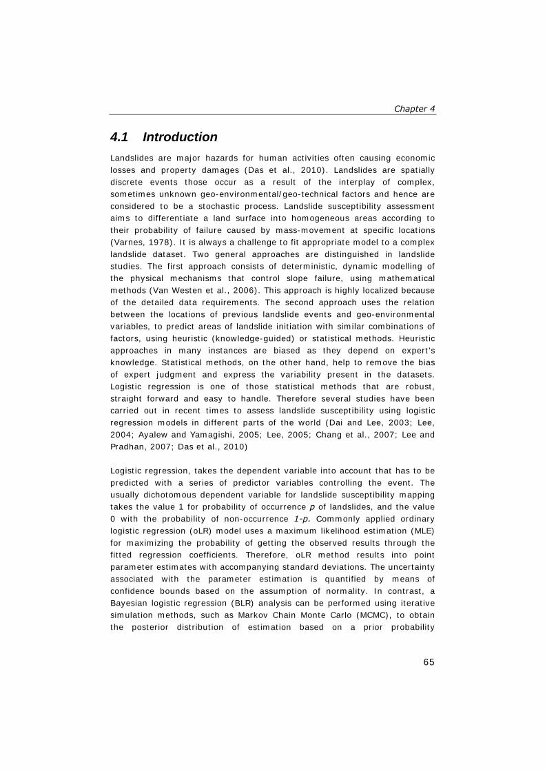
Chapter 4

65

4.1 Introduction Landslides are major hazards for human activities often causing economic losses and property damages (Das et al., 2010). Landslides are spatially discrete events those occur as a result of the interplay of complex, sometimes unknown geo-environmental/geo-technical factors and hence are considered to be a stochastic process. Landslide susceptibility assessment aims to differentiate a land surface into homogeneous areas according to their probability of failure caused by mass-movement at specific locations (Varnes, 1978). It is always a challenge to fit appropriate model to a complex landslide dataset. Two general approaches are distinguished in landslide studies. The first approach consists of deterministic, dynamic modelling of the physical mechanisms that control slope failure, using mathematical methods (Van Westen et al., 2006). This approach is highly localized because of the detailed data requirements. The second approach uses the relation between the locations of previous landslide events and geo-environmental variables, to predict areas of landslide initiation with similar combinations of factors, using heuristic (knowledge-guided) or statistical methods. Heuristic approaches in many instances are biased as they depend on expert’s knowledge. Statistical methods, on the other hand, help to remove the bias of expert judgment and express the variability present in the datasets. Logistic regression is one of those statistical methods that are robust, straight forward and easy to handle. Therefore several studies have been carried out in recent times to assess landslide susceptibility using logistic regression models in different parts of the world (Dai and Lee, 2003; Lee, 2004; Ayalew and Yamagishi, 2005; Lee, 2005; Chang et al., 2007; Lee and Pradhan, 2007; Das et al., 2010) Logistic regression, takes the dependent variable into account that has to be predicted with a series of predictor variables controlling the event. The usually dichotomous dependent variable for landslide susceptibility mapping takes the value 1 for probability of occurrence p of landslides, and the value 0 with the probability of non-occurrence 1-p. Commonly applied ordinary logistic regression (oLR) model uses a maximum likelihood estimation (MLE) for maximizing the probability of getting the observed results through the fitted regression coefficients. Therefore, oLR method results into point parameter estimates with accompanying standard deviations. The uncertainty associated with the parameter estimation is quantified by means of confidence bounds based on the assumption of normality. In contrast, a Bayesian logistic regression (BLR) analysis can be performed using iterative simulation methods, such as Markov Chain Monte Carlo (MCMC), to obtain the posterior distribution of estimation based on a prior probability


66

distribution, and maximum likelihood. In a Bayesian framework parameter estimates are no longer expressed as point estimates but instead are probabilistic, e.g. having probability distributions (Mila et al., 2003). Therefore, Bayesian methods provide an alternative to generally used frequentist methods, facilitating uncertainty estimation procedures. Being refined by the iterative simulation process, the BLR method shows higher accuracy of parameter estimates. The study aims to develop and apply a Bayesian logistic regression model for landslide susceptibility mapping. The Bayesian paradigm is used to modify the commonly applied frequentist logistic regression model. Uncertainty in parameter estimates is quantified by means of the posterior density distributions. The model consists of two steps. First, parameter estimates are obtained for each variable by means of oLR. The same variables are then used in a Bayesian framework for parameter estimation and the significance of each estimate is evaluated by means of the posterior density function obtained from the Bayesian analysis. Simulation of the model is done by iterative MCMC methods in WinBUGS. In the present study, ten different landslide influencing geo-environmental factors were analyzed in relation to the landslide occurrence data. The present study is a unique endeavour to carry out a logistic regression modelling in a Bayesian framework for landslide susceptibility mapping along with the uncertainty analysis of parameter estimates that has not been attempted so far. The results are validated by receiver operator characteristics (ROC) curve analysis using a separate set of landslide samples as training and testing data. The methodology is applied to a landslide-prone road corridor in the northern Himalayas in India.

4.2 Research Methods and Model In landslide studies a frequentist logistic regression model considers the occurrence of landslides as a discrete and dichotomous response variable, and the geo-environmental factors that influence it as explanatory variables (Das et al., 2010). In the present study the spatial relationships between landslide occurrence locations and landslide-related geo-environmental factors are identified. A bivariate statistical analysis is done to find out the relative importance of geo-environmental factors with respect to landslides. A routinely compiled oLR model is developed and applied to the dataset. The logistic regression model for k explanatory variables is formulated as:

⎥⎦⎤

⎢⎣⎡ +=+=+=== 1k

1j )ijxj0exp(/)k1j ijxj0exp()1iYPr(ip ∑∑ ββββ (4.1)

Chapter 4

67

where Pr(Yi = 1) is the probability of the occurrence of a landslide,

constrained to lie between 0 and 1, the ijx denote the different categories of

the geo-environmental factors and the βj, j = 0,…,k are unknown regression coefficients. Next, a Bayesian framework is constructed using the response and explanatory variable to account for the prior information as well as the data. A Bayesian framework contains three key components associated with parameter estimation: the prior distribution, the likelihood function and the posterior distribution. A simple Bayesian equivalent of the frequentist logistic model was constructed after Clark et al (2007).

))(logit(Bernoulli~y i1

i η− (4.2)

∑ =+=

k

1j ijj0i xββη

k,,0j),00001.0,0(N~j K=β

where iy represents the response variable, the βj’s are coefficients having

independent normal prior distributions with a very high variance,

ijx represents the value of the jth variable at ith location and iη is the linear

predictor. Using the Bayes formula, the posterior distribution of the parameters β under this model is given by:

∏∏==

×∝n

1iii

k

0jj )|yPr()Pr()X,y|( ηββπ (4.3)

where, ( )k10 ,...,, ββββ = ,

( )n21 y,...,y,yy = and

[ ] k,...,2,1j,n,...,2,1i,xX ij === .

This is an extension of the Bayesian formula )|( yf θ α )(θg × )|( θyL , which

relates the posterior distribution as proportional to the product of the prior distribution and the likelihood function (Fig. 4.1). Prior distribution Pr(βj). In this study noninformative priors are considered, because the aim is to show the advantage of a Bayesian method over


68

ordinary frequentist method using normal priors without using additional knowledge. Likelihood function Pr(yi|ηi). The geo-environmental variables are the ones that control landslide occurrences. Their inter-relationship with landslides gives inference about the significance of each variable.

Figure 4.1 Schematic representation of computational methodology. The iterative Bayesian method gives rise to a continuous distribution of parameter estimates in the form of pdfs as compared to point estimates by oLR model.

4.3 Site characteristics and database The area used to demonstrate the method lies between 300 47’ 29”N and 300 54’ 45”N latitude and 780 37’ 41”E and 78044’03”E longitude in the northern Himalayas, India in the catchment of the river Bhagirathi, a tributary of the river Ganges (Figure 4.2). The area is run through a national highway corridor connecting the famous Gangotri shrine of India in interior Himalaya. The area receives heavy precipitation during the summer months between July and September and moderate rainfall during the winter months between January to March (Figure 4.3). Elevation in the area ranges between 1550 and 2100 m and average annual rainfall is approx. 1200 mm (Vinod Kumar et al., 2008; Das et al., 2010). In the Himalayan region, landslides are recurring annually and are prominent during the summer months between July and September. Landslides in this area are the result of the combination of an intrinsic geology, adverse natural topography like steep slopes, weathered

Chapter 4

69

rocks and soils, human influences on the topography and high rainfall (Choubey and Ramola, 1997; Saha et al., 2005).

Figure 4.2 Location and extent of the study area as depicted on a hill shade image generated using a DTM derived from a Cartosat-1 satellite image. The highway runs along the Bhagirathi River in the Himalayas, India.

4.3.1 Landslide identification and mapping A correct landslide database is the pre-requisite for any kind of landslide study (Varnes, 1984). A combination of various sources, means and methods has been suggested for landslide inventory mapping, as no single best method for landslide inventorization exists (Galli et al., 2008; van Westen et al., 2008). A detailed landslide inventory for susceptibility assessment requires mainly the following data input: the location of a landslide, its frequency, potential causes of a landslide and the type of landslide. For the precise landslide identification, accurate landslide mapping and the collection of landslide data from reliable sources plays an important role. The major organizations which keep the updated record of landslides in the Indian Himalayan terrain are the Border Road Organization (BRO) and the Geological Survey of India (GSI). The landslide records in the form of digital catalogues of the BRO compiled between 1982 and 2009 were used in this study for preparing the inventory. The BRO catalogue consists of three types of records: (i) Register of landslides (RLS), a Decadal report on each landslide hitting the road, (ii) History of landslides (HLS), a quarterly report on significant landslides and (iii) Daily road stirrup (DRS), a report on the reasons of road blockage. All these three types of records were checked simultaneously to compile the landslide database for last 28 years which consists of 380 records of landslide occurrences. The technical records of BRO


70

provided a detailed description of landslide location, morphometry, volume and date of occurrence of landslides. This helped us in identifying the morphological imprints left by the landslide scars on the road corridor leading to detection of landslides. Compilation of records also helped us in identifying the reactivated landslides with little difficulty as well as the frequency of landslides occurring in a particular location. In addition multiple satellite images acquired from Resoucesat-1, Cartosat-1, Landsat-TM, IRS-1C and 1D satellite were also interpreted visually for deriving geomorphic signatures of landslides.

Figure 4.3 Mean monthly rainfall values (left y-axis) and percentages (right y-axis) for the period between 1982 and 2009 for the Bhatwari rain gauge station 1550m above mean sea level.

Chapter 4

71

Figure 4.4 The landslide inventory map of the study area showing dominance of rockslides. The 178 landslides experienced a total of 332 occurrences during 1982 to 2009. Extensive field verification was carried out in consultation with the BRO to map the landslides in the study area. A total of 178 active landslides were mapped at the 1:10,000 scales. These were correlated with the BRO records in their digital catalogue of landslides for the road corridor occurring along the cut slopes, as well as in the natural slopes of the road corridor (Figure 4.4). Slide events along these active sites were reported 332 times in the last 28 years, with a maximum of 60 occurrences in 1994 (Figure 4.5). Landslides in the study area are mostly triggered by monsoon rainfall during July to October every year. The landslides were characterized according to their types of movements, the materials involved and the states or activities of failed slopes (Cruden and Varnes, 1996). This was done to understand different geo-environmental factors that control different slope movement types. Field observations revealed that the area is dominated by rock and debris slides (Figure 4.6). Accordingly, the landslides considered in this study


72

are mainly translational rock slides and debris slides that are prominent in this area (Das et al., 2010). The materials involved in majority of landslides are a mixture of rocks, pebbles, gravels and cobbles. Landslide bodies were mapped from crown to toe of rupture, as the detachment zones (zone of depletion) are the true susceptible areas, leaving aside the runout zones. We described landslide types according to Cruden and Varnes (1996). The annual summer monsoon in the area during June to October triggers both fresh as well as reactivated landslides. Changes in the water level of the main stream, the Bhagirathi river, also influences toe cutting, resulting in few landslides in the road corridor. Landslides on the cut slopes of the road corridor are smaller in size but occur frequently. A record of every landslide affecting the road corridor is logged by BRO. The mapped landslides cover an area of 0.45 km2, corresponding to 5.6% of the total area (min. 125 m2, max. 40,500 m2 and mean 3,967 m2). As the overall landslide density was low in the area, we considered all landslide types together for the susceptibility modelling.

Figure 4.5 Histogram showing the frequency of landslide occurrence (left y-axis) and percentages (right y-axis) for the period between 1982 and 2009

Chapter 4

73

Figure 4.6 Landslides occurring along the road corridor, (A) a large rock-cum-debris slide damaging the houses and the road (B) a rock slide blocking the road partially

4.3.2 Landslide influencing factors Efforts were made to carry out a detail mapping of the study area using satellite images and multiple field surveys to ascertain the nature of terrain and the factors that influence landsliding. This is because the geo-environmental factors influencing landsliding are not uniform throughout the world. The general consensus is that any geo-environmental variable should have a logical, rational and technical bearing on the landslides in a particular area (Ayalew and Yamagishi, 2005). Landslides in our area are initiated from natural as well as cut slopes of the road corridor. We carried out a logistic regression model based susceptibility study for the landslides along the cut slopes of the road and compared it with the output of rock mass rating based slope stability probability classification (SSPC) method (Das et al., 2010). However, to account for all the landslides in the road corridor including the ones initiating in the natural slope beyond road section and to improve upon the oLR model, knowledge guided data driven method of BLR is proposed. In this model we have included road buffer as one of the additional geo-environmental factors besides the nine factors such as slope, lithology, terrain units, landcover, soil depth, weathering, aspect, drainage density and


74

geological structures (lineament density) considered for earlier study. This is done to account for the road cuts as one of the factors in controlling landslides in the entire corridor. Each factor is divided into a number of discrete classes that are likely to affect landslide occurrence. The rock types in the study area include low to high grade metamorphics (green-schist to upper amphibolite facies) which have been deformed repeatedly (Naithani et al., 2009). On the basis of metamorphic grades the rocks of this area are divided into three parts viz. Lower, Middle and Upper crystallines (Purohit et al., 1990). The lower crystalline constitutes low grade metamorphic rock such as chlorite schist, schistose quartzite and quartz mica schist. The middle crystalline constitutes varying types of migmatites such as gneissic, banded migmatites and biotite gneisses. The upper crystalline rocks are represented by medium to high grade of metamorphism as evidenced by the presence of augen-gneiss, and calc-silicate-gneiss. To assess the relationship between lithology and landslide in the area a bivariate statistical analysis (BVA) was carried out using eight lithology classes and landslides (Figure 4.7). This was done in GIS environment by comparing the rasterized map of lithology and landslide inventory. Landslide density in each lithology class was obtained by first calculating the ratio between the areas occupied by landslide cells in a particular class to the total area of that class. The ratios calculated for each class of the factor map were added and each ratio was divided by the total sum of the ratios. Table 4.1 presents the landslide densities computed for the geo-environmental factor maps used for landslide susceptibility assessment. The lithology class representing calc silicate gneiss has the highest landslide density. Landslide density is also higher in the classes like quartz mica schist and schistose quartzites. This is one of the indications that the rock mass parameters of these lithologies may be favourable for landsliding.

Chapter 4

75

Figure 4.7 Geological map of the study area showing the lineaments and the eight categories of litho-types identified through rock mass characterization. Table 4.1 Landslide densities computed for the geo-environmental factor maps used for landslide susceptibility assessment

Factors Variables Landslide

density (%)

Lithology

Biotite-Gneiss 14.87 Migmatite Gneiss 5.15 Calc-Silicate Gneiss 26.21 Chlorite Schist 10.16 Quartzite 1.91 Quartz mica schist 20.97 Augen Gneiss 2.03 Schistose Quartzite 18.70

Terrain unit

Intermontane valley wide 6.21 Intermontane valley narrow 4.34 Massive type poorly dissected denudational hills 14.23 Ridge type highly dissected hills 18.05 Cuesta type mod. dissected denudational hills 24.12 Hog back type highly dissected structural hills 21.92 Dome type moderately dissected denudation hills 11.13

Lineament Density

Low 12.34 Moderate 43.23 High 44.43


76

Table 4.1 continued...

Geotechnical investigations were carried out in the area using SSPC method (Das et al., 2010). The entire road stretch of 12 km was divided into 32 slope sections and the geotechnical data were collected quantitatively for determining the rock mass parameters required in SSPC system (Das et al., 2010). Rock mass properties such as intact rock strength (IRS), discontinuity spacing and condition, were tabulated in the field. Gneisses constitute 87% of the total study area. Twenty field measurements taken in the gneissic areas showed that the IRS varies between 50 to 200 MPa (Figure 4.8) and the cohesion of rock mass for the same locations varies between 18-29 KPa. A detail observation showed that IRS is higher in migmatite and biotite gneisses in comparison to the calc-silicate and augen gneisses. This may be because of the spacing and orientation of the joints present in these rocks and the degree of weathering. Rocks are jointed and four sets of joints

Factors Variables Landslide

density (%)

Land cover

Scrub land 28.23 Dense forest 11.32 Agricultural land 9.24 Barren land 22.35 Sand area 0 Built-up land 2.54 Degraded forest 19.87 Open Forest 6.45 River channel 0

Soil depth Very shallow 0 Shallow 37.32 Moderate 33.73 Deep 28.95

Weathering


Aspect

North 3.76 North East 7.25 East 14.28 South East 15.71 South 21.33 South West 20.45 West 11.10 North West 6.10

Slope

1-15 deg 03.38 15-25 deg 11.25 25-35 deg 16.22 35-45 deg 42.67 45-60 deg 15.23 >60 deg 11.25

Drainage density


Road buffer Road buffer 63.2 Outside road buffer 36.8

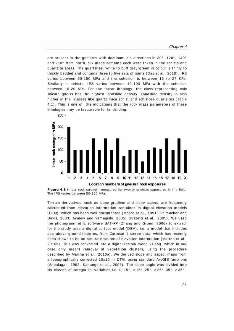
Chapter 4

77

are present in the gneisses with dominant dip directions in 30°, 120°, 140° and 210° from north. Six measurements each were taken in the schists and quartzite areas. The quartzites, white to buff grey/green in colour is thinly to thickly bedded and contains three to five sets of joints (Das et al., 2010). IRS varies between 50-150 MPa and the cohesion is between 15 to 27 KPa. Similarly in schists, IRS varies between 10-100 MPa with the cohesion between 10-20 KPa. For the factor lithology, the class representing calc silicate gneiss has the highest landslide density. Landslide density is also higher in the classes like quartz mica schist and schistose quartzites (Table 4.1). This is one of the indications that the rock mass parameters of these lithologies may be favourable for landsliding.

Figure 4.8 Intact rock strength measured for twenty gneissic exposures in the field. The IRS varies between 50-200 MPa. Terrain derivatives, such as slope gradient and slope aspect, are frequently calculated from elevation information contained in digital elevation models (DEM), which has been well documented (Moore et al., 1991; Ohlmacher and Davis, 2003; Ayalew and Yamagishi, 2005; Guzzetti et al., 2005). We used the photogrammetric software SAT-PP (Zhang and Gruen, 2006) to extract for the study area a digital surface model (DSM), i.e. a model that includes also above-ground features, from Cartosat-1 stereo data, which has recently been shown to be an accurate source of elevation information (Martha et al., 2010b). This was converted into a digital terrain model (DTM), which in our case only meant removal of vegetation clusters, using the procedure described by Martha et al. (2010a). We derived slope and aspect maps from a topographically corrected 10x10 m DTM, using standard ArcGIS functions (Anbalagan, 1992; Kanungo et al., 2006). The slope angle was divided into six classes of categorical variables i.e. 0–15°, >15°–25°, >25°–35°, >35°–


78

45°, >45°–60° and >60° (Figure 4.9). It may be argued that the slope can be considered as a continuous variable rather than a six class categorical variable. However in the steep slopes of northern Himalayan road corridor with a complete set of landslides records sufficient knowledge have been gained for optimally classifying the slope conditions. In addition logistic regression model is capable of handling categorical data effectively. The slope class (>35°-45°) has the highest landslide density in the study area (Table 4.1). The highest landslide density was observed on slopes with southern aspect, followed by south-west aspect (Table 4.1). Road construction severely alters the slope stability in hilly areas, increasing the susceptibility to slope instability and landslides (Chakraborty and Anbalagan, 2008). The best way to include the effect of a road section in a slope stability study is to make a buffer around them (Larsen and Parks, 1997; Ayalew and Yamagishi, 2005). Extent of slope cuttings due to road construction was mapped using field investigation. Landslide frequency in the study area was observed to be highest within about 100 meters around the narrow road (average width of 7 m). Thus a road buffer of 50 m was placed on either side of the road centre, marking the area likely influenced by cutting-related slope instability. Other landslide influencing topographic parameters in the area, such as soil depth, terrain geomorphic units, land cover, drainage density and weathering conditions, were derived using ground surveys and interpretation of multi-temporal satellite images detailed in Das et al. (2010).

Chapter 4

79

Figure 4.9 The slope map of the study area

4.4 Implementation In this study we used the GLM module in the R software package to fit equation 1 to the data for oLR model. Logistic regression modelling uses variable proportions of 1 (“landslide”) and 0 (“no-landslide”) grid-cells for model development (Ayalew and Yamagishi, 2005). In the present study, 2254 grid-cells containing landslides (50 % of the total 4508 slide-cells), along with an equal number of non-landslide cells, selected randomly from landslide free areas, were considered in building the model (Yesilnacar and Topal, 2005; Mathew et al., 2009). Rest 50% of the landslide cells have been retained for accuracy assessment. The landslide cells were converted to logical variables representing “true” or “false” for “landslide” or “no-landslide”, respectively. The explanatory variables corresponding to true and false slide-cells were represented in categorical form like A, B, C etc. After that the generalized linear model with the logit link function was used for logistic regression. The model resulted in parameter estimates, standard errors, and the level of significance of each estimate for intercept and


80

coefficients. The key items in this output were the level of significance values for the interactions that indicate the degree of contribution of the variables to the model. Null deviance and residual deviances were checked for the significance of the model (Das et al., 2010). Bayesian analysis was carried out using WinBUGS programme 3.0.3 © 1989, 1991 Free Software Foundation, Inc. 59 Temple Place - Suite 330, Boston, MA 02111-1307, USA). Input landslide and geo-environmental factors data were exactly same as for the oLR modelling. The data were first converted into ASCII format for inputting into the WinBUGS software to create dummy variables. The GLM programme in WinBUGS was used for the Bayesian analysis of the data. Monitoring convergence of simulation is an important step in a Bayesian analysis, because only the iterations after convergence are used to obtain estimates of parameter distribution, such as mean, median, standard deviation and quantiles. Checking convergence was done by running two chains simultaneously and, observing their live trace plots as well as the history of trace plots. After the simulation converged, the trace plots showed the overlap of two chains and pdfs were generated for each parameter (Figure 4.10). The Monte Carlo error in the summary statistics was obtained for initial simulations in regular intervals and cross checked with standard deviation. Hence, initially the simulations were run in 1000’ iterations and then in 5000’s for 25,000 iterations. After checking the multiple runs, further 25,000 iterations were carried out to generate posterior summaries of parameter statistics (Brooks and Gelman, 1998). The statistical summaries were presented in table 4.2. The Brook, Gelman and Rubin (BGR) statistics also indicated that there was convergence of the chains. The more simulations are run after convergence, the more the parameters get refined. After a certain number of iterations the changes become insignificant. In the present case, 25,000 and 75,000 iterations after convergence resulted in negligible differences in terms of parameter statistics.

Chapter 4

81

Figure 4.10 History of trace plots and density distribution of the corresponding posterior parameter estimates (pdfs of beta’s) for 2 selected variables (A & B). History of trace plots indicate the parameter value after 25,000 iterations for convergence of simulation.

4.5 Results and discussion The results of oLR and BLR are presented in table 4.2. The seventeen variables contributing significantly to the landslide occurrences are ‘slope category >35°-45°’ for the factor slope, ‘calc-silicate gneiss’, ‘biotite gneiss’, ‘migmatite gneiss, and ‘schistose quartzite’ for factor lithology, ‘scrubland’, and ‘river channel’ for the factor landcover, ‘South-East’, and ‘South’ for the factor Aspect, ‘HTHDSH’, and ‘CTMDSH’ for the factor geomorphology, ‘deep’, and ‘shallow’ for factor soil depth, ‘high’ weathering, ‘high’ drainage density, ‘lineament buffer zone’ and ‘road buffer zone’ respectively. Many categories in the geo-environmental factor maps, did not contribute significantly to the model output. This may be because the variables are not conditionally independent with each other, or they do not contribute significantly to the response variable.


82

Table 4.2 Point estimates of ordinary logistic regression analysis and posterior distribution summaries of parameter estimates of Bayesian logistic regression model for landslide occurrence with reference to significant geo-environmental variables Variables Point

estimate from oLR

Mean of Parameter posterior estimate

Standard deviation of

posterior distribution

Quantiles of posterior distribution

2.5% Median 97.5%

Intercept -2.265 -1.531 0.483 -3.392 -1.433 -0.481 Slope gradient: >35-45 degree

0.531 0.239 0.127 0.002 0.288 0.582

Lithology: Calc-silicate gneiss

0.836 0.454 0.187 -0.253 0.467 0.925

Lithology: Biotite gneiss

-1.386 -1.182 0.342 -2.123 -1.098 0.254

Lithology: Migmatite gneiss

-1.023 -0.453 0.227 -1.654 -0.483 -0.050

Lithology: Schistose quartzite

0.324 0.436 0.3141 -0.179 0.431 1.057

Terrain units: HTHDSH (Hogback type highly dissected structural hills)

1.699 1.205 0.405 0.616 1.352 2.207

Terrain units: CTMDDH (Cuesta type moderately dissected denudational hills)

2.764 1.215 0.404 0.812 1.255 2.4

Landcover: Scrub land

0.690 0.894 0.210 0.297 0.826 1.899

Landcover: River channel

-0.876 -0.763 0.178 -1.106 -0.760 -0.424

Soil depth: deep -0.976 -0.762 0.347 -2.63 -0.755 -0.457 Soil depth: shallow -2.123 -2.546 0.240 -3.889 -2.422 -1.946 Weathering: High 2.131 2.053 0.304 1.511 2.110 3.911 Aspect: South-east 1.534 2.830 0.305 1.228 2.824 3.478 Aspect: South 1.814 2.013 0.320 1.464 2.107 2.707 Drainage density: high

0.500 0.700 0.150 0.154 0.654 0.940

Lineament density: high

0.508 0.529 0.128 -0.166 0.608 1.252

Road buffer 0.500 0.445 0.150 0.154 0.445 0.740

Interpretation of the coefficients from the logistic model is not as straightforward as interpretation of the coefficients in a linear model, and therefore we turn towards their exponential values. For example, the estimated coefficient of the parameter ‘slope >35–45°’ equals 0.531, whereas its exponential value equals 1.70 for the oLR model. Therefore, for a cell that is not in the >35–45° slope category to have a 0.5 probability of a landslide occurrence the corresponding odds of the slide are 1. If the cell falls within the >35–45° slope category, however, the odds become 1.70. As a consequence the probability of a slide changes to 0.629, being approximately 26% higher than the initial probability of 0.5. On the other hand for the same variable ‘slope class >35°-45°’ the BLR model generates the parameter mean value 0.239. Therefore, for BLR model the odds become 1.269. Hence the

Chapter 4

83

probability of a slide changes to 0.559, i.e. 12% higher than the initial probability of 0.5 with the end points of 95 percent confidence interval estimation as 0.002 and 0.582. The distribution of the estimation also indicates that the change in the log-odds of landslide for this slope class are between 0.002 and 0.582 with 95% confidence and the parameter estimate is contributing positively to the landslide occurrences. Comparing the posterior estimates of the BLR model with those of the oLR model highlighted several interesting issues. - The variable ‘slope category >35°-45°’ indicates that in Himalayan

conditions the area is prone to occurrence of landslides and both model outputs are in agreement in terms of their positive parameter estimates. The BLR model further indicates that it is very unlikely (< 5%) that the parameter estimate is beyond the range of 0.002-0.582.

- Contributions from significant lithology classes are a clear indication of the impact of rock types and rock strength on landslide occurrence in the area and both models agree to it. Calc-silicate gneiss and schistose quartzite have positive parameter estimates indicating that the rock types contribute to the landsliding. However, the 95% confidence interval for calc-silicate gneiss varies between -0.253 and 0.925 indicating a chance of negative contribution from a particular lithology class. Such is also in the case of schistose quartzite. On the other hand, biotite gneiss and migmatite gneiss have negative parameter estimates indicating stabilization. However, the confidence interval values can be interpreted in similar ways.

- Two significant geomorphology classes, HTHDSH and CTMDDH, contribute positively to the landslide occurrence probability. Further, the BLR model indicates that in 2.5% cases their parameter estimate can be below 0.616 and 0.812, respectively.

- Contributions from significant aspect classes (South-East and South) to the mean parameter estimates of the BLR model are again in a one-to-one agreement with the point estimates of the oLR model. This is because the sun facing slopes in the Himalayas are less vegetated and more prone to landslides.

- Lineaments, mainly the major rock fractures in the present study, contribute positively to landslide occurrence when their density is high. However, the BLR model clearly indicates a small probability (2.5%) that the parameter estimate for this class can have a negative coefficient (-0.166).

- Roads have a strongly positive effect on landslide incidence, confirmed by both the models, a fact well documented in the Himalayas.


84

Other coefficients can be interpreted in the same way for the log-odds as well as for their negative and positives estimates. Bayesian estimation, thus, is not in conflict with oLR estimation, but rather provides another technique that can incorporate iterative simulation to provide a finer set of inferences about the parameter estimates. This is because the posterior parameter estimates for BLR model are obtained by iterative simulation as the posterior mean of parameter estimation in case of BLR is derived from a distribution, whereas the output of oLR is a point estimate (Mila et al., 2003). After interpreting the results from both oLR and BLR model, logit formulas were created for both the models using significant variables. ηi = -2.265 + 0.531 slope (>35°-45°) + 0.836 calc-silicate gneiss + (-1.386) biotite gneiss + (-1.023) migmatite gneiss + 0.324 schistose quartzite + 1.699 HTHDSH + 2.764 CTMDDH + 0.690 scrubland + (-0.876) river channel + (-0.976) deep soil+(-2.123) shallow soil+ 2.131 high weathering + 1.534 Aspect (SE) + 1.814 Aspect (S) + 0.5 high drainage density + 0.508 Lineament density +0.5 Road buffer (4.4) ηi = -1.531 + 0.239 slope (>35°-45°) + 0.454 calc-silicate gneiss + (-1.182) biotite gneiss + (-0.453) migmatite gneiss + 0.436 schistose quartzite + 1.205 HTHDSH + 1.215 CTMDDH + (0.894) scrubland + (-0.763) river channel + (-0.762) deep soil+(-2.546) shallow soil+ 2.053 high weathering + 2.83 Aspect (SE) + 2.013 Aspect (S) + 0.7 high drainage density + 0.529 high lineament density +0.445 road buffer (4.5) Using these estimated logit for oLR and BLR model respectively, each combination of explanatory variable values were filled in the Eq. (4.1) and Eq. (4.2) respectively and the susceptibility maps were created and compared

4.5.1 Landslide spatial probability (susceptibility) map To compare the two output maps they were divided into equal number of classes with identical interval. The final resultant probability maps were shown in Figure 4.11. As shown in table 4.3 and the resultant probability maps, the prediction in the low probability range between 0.0 – 0.25, covers a larger area using the BLR model than using the oLR model. Similarly, in the high probability range of >0.5 – 0.75, the BLR model also predicted a larger area. However, the BLR model was conservative in predicting very high class (>0.75 – 1.0) as the area percentage almost matches the percentage of landslide in the study area (5.25% predicted versus 5.6% actual). On the other hand oLR model had a higher prediction percentage i.e. 9.87% in this

Chapter 4

85

class. This clearly signifies the advantage of an iterative Bayesian model over an ordinary frequentist model, which is also clear from the true and false positive analysis, and the AUC of receiver operator characteristic (ROC) curve.

Figure 4.11 Landslide susceptibility maps. (A) Generated using ordinary logistic regression. (B) Generated using Bayesian logistic regression. Table 4.3 Area distribution of each landslide probability class in the study area

Probability value range Area (%) using oLR

model Area (%) using BLR

model

0.0 - 0.25 (Low) 16.18 22.15 >0.25 – 0.50(Moderate) 46.09 41.37

>0.50 – 0.75 (High) 27.86 31.23 >0.75 – 1.0 (Very high) 9.87 05.25

4.5.2 Model validation and accuracy assessment By using the Receiver operation characteristic (ROC) curve, success was assessed by comparing the calculated probability values vis-à-vis their actual present condition. True positive rates (sensitivity) are compared against false positive rates (1-specificity) to assess the prediction accuracy by the models. The ROC curve is shown in Fig. 4.12. The area under the curve (86.0% for BLR and 79.6% for oLR model) implies a higher success rate for BLR model, even with same set of variables. Further, the ROC curve shows a more rapid


86

increase in the initial stage of the BLR model as compared to the oLR model. This indicates the higher sensitivity of the BLR model to the output probability. Above all, the probability map generated by means of the BLR model better classifies the data and the success rate is higher compared to the oLR model for same set of variables. The BLR model is also validated by using 50% of the landslide cells separately kept for validation. The 2,254 landslide cells which have not been used in developing the model, along with an equal number of randomly selected non-landslide cells have been used for the ROC curve analysis. It shows the area under the curve is 0.839, which corresponds to an accuracy of 83.9% for the model developed using Bayesian logistic regression (Figure 4.12). The standard error in the ROC curve in all cases is less than 0.005.

Figure 4.12 Three ROC curves representing true positive rates (sensitivity) and false positive rates (1-specificity) for oLR model (black-dots line), BLR validation (dash line) and BLR model (solid line). Area under the curve (AUC) values is 0.796, 0.839 and 0.860 respectively.

Chapter 4

87

4.6 Conclusions This study presents a Bayesian logistic regression model for landslide susceptibility modelling. Results of the model showed that uncertainty analysis in parameter estimates can be comprehensively addressed using this method with a detail statistical output. This is because the Bayesian method performs iteratively, resulting in a probability distribution of the posterior estimates of the parameters through pdfs. Also it has the advantage of prior information being included in the analysis. Predictive probability values obtained through BLR model thus shows higher success rates for landslide susceptibility mapping. A logistic regression model in a Bayesian framework has the advantage of analyzing the parameter uncertainty from a probability distribution of the posterior estimates in a more realistic way than an ordinary logistic regression model. We concluded that, being performed iteratively, the BLR model allows the analysis of uncertainty information by means of a probability distribution that is generally lacking in an ordinary logistic regression method. The Himalayan road corridor example clearly illustrated this. The Bayesian estimation of parameters discussed here can be applied to any database characterizing inherent properties of landslides. The methodology may be applicable to different hazards, such as earthquakes, with other explanatory variables, but within the same Bayesian logistic framework.


88

89

5. Landslide hazard assessment using homogeneous susceptible units (HSU)

5.1. Introduction 5.2. Methods 5.3. Study area and landslide characterization 5.4. Hazard assessment 5.5. Discussion and conclusions

Earth provides enough to satisfy every man’s need, but not every man’s

greed.

Mahatma Gandhi This chapter is based on

Das, I., Stein, A., Kerle, N. and Dadhwal V.K. (2011[in press]). Probabilistic landslide hazard assessment using homogenous susceptible units (HSU) along a national highway corridor in the northern Himalayas, India. Landslides, DOI 10.1007/s10346-011-0257-9.

Landslide hazard assessment using homogeneous susceptible units

90

Abstract The increased socio-economic significance of landslides has resulted in the application of statistical methods to assess their hazard, particularly at medium scales. These models evaluate where, when and what size landslides are expected. The method presented in this study evaluates the landslide hazard on the basis of homogenous susceptible units (HSU). HSU are derived from a landslide susceptibility map that is a combination of landslide occurrences and geo-environmental factors, using an automated segmentation procedure. To divide the landslide susceptibility map into HSU we apply a region-growing segmentation algorithm that results in segments with statistically independent spatial probability values. Independence is tested using Moran’s I and a weighted variance method. For each HSU we obtain the landslide frequency from the multi-temporal data. Temporal and size probabilities are calculated using a Poisson model and an Inverse-gamma model, respectively. The methodology is tested in a landslide-prone national highway corridor in the northern Himalayas, India. Our study demonstrates that HSU can replace the commonly used terrain mapping units (TMU) for combining three probabilities for landslide hazard assessment. A quantitative estimate of landslide hazard is obtained as a joint probability of landslide size, of landslide temporal occurrence for each HSU for different time periods and for different sizes. Keywords: Landslides; Hazard, HSU, Segmentation, Himalayas, India.

Chapter 5

91

5.1 Introduction Landslides are events that pose a major hazard for human activities, and that often cause substantial economic losses and property damages (Nadim et al., 2006; Hong et al., 2007). Landslides, in a strict sense, are the movement of a mass of rock, debris or soil along a downward slope, due to gravitational pull. A variety of movements is associated with landslides, such as flowing, sliding (translational and rotational), toppling or falling. Many landslides exhibit a combination of two or more types of movements, resulting in a complex type (Varnes, 1984). They are triggered by a number of external factors, such as intense rainfall, earthquake shaking, water level change, storm waves and rapid stream erosion etc. (Dai et al., 2002). In addition extensive human interference in hill slope areas for construction of roads, urban expansion along the hill slopes, deforestation, and rapid change in land use contribute to instability. This makes it difficult, if not impossible, to define a single methodology to identify and map landslides, to ascertain landslide hazards, and to evaluate the associated risk (Guzzetti et al., 2005). It thus necessitates a detailed understanding of the physical process of landslides, including historical information on their occurrence. Growing environmental concern in recent years has resulted in a range of quantitative landslide hazard and risk assessment studies (Alexander, 2008; Carrara and Pike, 2008). The assessment of landslide hazard has become an important assignment for various interest groups comprising technocrats, planners and others, mainly due to an increased awareness of the socio-economic significance of landslides (Devoli et al., 2007). So far, a number of methods has been proposed for quantitative landslide spatial probability mapping, e.g. discriminant analysis (Baeza and Corominas, 2001), likelihood ratio (Chung and Fabbri, 2003), ANN (Kanungo et al., 2006) and logistic regression (Lee and Pradhan, 2007; Das et al., 2010). However, actual methodological developments for quantitative hazard analysis have been scarce, particularly in medium scales (Guzzetti et al., 1999; Van Westen et al., 2006). Except for a limited number of studies (Zezere et al., 2004; Guzzetti et al., 2005; Hong et al., 2007), most of the methods proposed as landslide hazard modelling can best be classified as susceptibility models, as they only provide the estimate of where landslides are expected (Guzzetti et al., 2005). Varnes (1984) was the first to propose the definition of landslide hazard as “the probability of occurrence within a specified period of time and within a given area of a potentially damaging phenomenon”. This definition includes two parameters: the geographical locations (where) and the recurrence between events (when) of the landslides. Later the magnitude of the event was added to the definition of landslide hazard by Aleotti and Choudhury


92

(1999) and Guzzetti et al. (1999). Quantifying landslide hazard thus necessitates the determination of magnitude probability, along with spatial probability (susceptibility) and temporal probability. We notice that estimating where and when landslides occur is comparatively straightforward, whereas estimating magnitude is difficult. This is because, unlike other natural hazards such as floods, cyclones and earthquakes, which are controlled by rainfall, wind speed and ground motion respectively, landslides lack a spatially continuous magnitude measurement parameter. It may be argued that landslide magnitude is a function of the momentum, which includes both mass (volume and density) of the landslide material and the expected velocity. However, volume and velocity are difficult to evaluate in a medium scale for large areas. Nevertheless, landslide area can be precisely determined from a multi-temporal inventory map (Guzzetti et al., 2005). Therefore, landslide area can act as a good approximation for landslide magnitude. Landslide susceptibility mapping aims to differentiate a land surface into homogeneous areas according to their probability of failure caused by mass-movements (Varnes, 1984). To achieve this objective at medium scales, terrain mapping units (TMU) are generated to evaluate the suitability of landslide occurrence in an area on the basis of such homogeneous conditions (Carrara et al., 1991; Carrara et al., 1995; Soeters and van Westen, 1996; Pasuto and Soldati, 1999). Further, the use of mapping units is also common in landslide hazard assessment purposes. These are, in principle, homogeneous internally and heterogeneous externally. With increasing sophistication of GIS, TMU are either derived automatically from a combination of geo-environmental factors or semi-automatically using expert knowledge (van Westen et al., 1997). As they are generated independently, i.e. without incorporation of landslide occurrences, TMU fall short of representing actual homogenous susceptible areas. Instead, they can at best represent homogenous terrain conditions with respect to certain geo-environmental factors that control landslides. Further, combining multiple geo-environmental factors to generate TMU can result in an uncontrolled number of units. Therefore, segmentation-based homogenous susceptible units (HSU), which can be generated automatically from a susceptibility map using a region growing algorithm, may be considered as an alternative to TMU. The HSU can address the inherent homogeneity conditions of factors with respect to landslides, and can suitably replace the TMU for hazard assessment. The aim of this study is to develop and apply a quantitative methodology for landslide hazard assessment using HSU. We derive the HSU automatically

Chapter 5

93

from a grid-based susceptibility map using a region growing algorithm and an optimal size factor. The temporal and size probabilities are multiplied with spatial probability to obtain a quantitative estimate of landslide hazard for each HSU. We test the methodology using a multi-temporal landslide inventory in a national highway corridor in the Himalayan region.

5.2 Methods A probabilistic landslide hazard assessment procedure demands the determination of three distinct components of hazard assessment, namely spatial, temporal and size probability (Guzzetti et al., 2005). The spatial probability is generally calculated by considering landslide locations and their spatial interaction with geo-environmental factors. This is a measure of spatial locations where landslides may occur in the future. Similarly, temporal probability expresses the frequency of occurrence of landslides in a given period. The size probability of landslides is determined from a sufficiently complete landslide record, and indicates the probability of particular size of landslide to occur. Mathematically, if the probability of the size of a landslide

is denoted by LAP and the probability of occurrence of a landslide in a period

t by tP , in a HSU at a spatial location i with probability Pi, then the joint

probability of landslide hazard (H) can be represented as

LAti PPPH ××= (5.1)

5.2.1 Spatial probability (susceptibility) modelling and generation of HSU

The spatial probability of landslide occurrence can be modeled as the probability that a particular area will be affected by landslides, given a set of environmental conditions. In statistical techniques, such as logistic regression models, the occurrence of landslides is considered as a discrete and dichotomous response variable, and the geo-environmental factors that influence it as explanatory variables; for more details see Das et al. (2010). A logistic regression in a Bayesian framework uses three key components, the prior distribution, the likelihood function and the posterior distribution, for estimating the regression parameters. The Bayesian logistic regression model used for the calculation of regression coefficients takes the following form:

(5.2)

)1y(PP ii ==

))(logit(Bernoulli~y i1

i η−∑ =+=

k

1j ijj0i xββη


94

k,,0j),00001.0,0(N~j K=β

where iy represents the response variable, the βj’s are coefficients having

independent normal prior distributions with a very high variance,

ijx represents the value of the jth variable at ith location and iη is the linear

predictor. Using the Bayes formula, the posterior distribution of the parameters β under this model is given by:

∏∏==

×∝n

1iii

k

0jj )|yPr()Pr()X,y|( ηββπ (5.3)

where, ( )k10 ,...,, ββββ = ,

( )n21 y,...,y,yy = and

[ ] k,...,2,1j,n,...,2,1i,xX ij === .

This is an extension of the Bayesian formula )y|(f θ α )(g θ × )|y(L θ ,

which relates the posterior distribution as proportional to the product of the prior distribution and the likelihood function. The βj’s are the mean of the parameter posterior estimates representing the regression coefficients as in case of an ordinary logistic regression for each variable. The analysis was carried out in WinBUGS programme 3.0.3. The GLM programme with the logit link function in WinBUGS was used for the Bayesian logistic regression analysis of the data. To assess the prediction rate of the model a receiver operator characteristic (ROC) curve analysis is carried out. This is a representation of the trade-off between sensitivity and specificity (Gorsevski et al., 2000). Sensitivity is the probability that a landslide cell is correctly classified, a true positive rate, whereas 1 – specificity is the false positive rate.

Generation of HSU through segmentation Segmentation is a process of dividing a raster image/map into objects or regions based on the homogeneity conditions of the adjacent pixels. It can be done in different ways, using various techniques such as density slicing, region growing, and split and merge (Kerle and de Leeuw, 2009). We carried out multiresolution segmentation using region growing algorithm in Definiens Developer, which is guided through the use of scale and shape parameters (Definiens, 2009). To divide a susceptibility map into an optimal number of HSU is a challenge, since such optimisation should satisfy homogeneity

Chapter 5

95

conditions that are in practice highly variable. In a strict sense true homogeneity in nature is almost impossible. Multiresolution segmentation is an option that generates segments of different size, and where the user has the option to choose optimal segment size (Baatz and Schape, 2000). To choose such an optimal segment size objectively, Espindola et al. (2006) proposed an objective function for measuring the quality of the resulting segments. Therefore, we created segments/objects of different scale parameters, with thresholds ranging from 10 to 50. The scale parameter is a function used to control the maximum allowed heterogeneity of the objects in generating segments, resulting in a higher number of segments for lower scale. To assess the quality of segments and decide upon the optimal segment size, an independency test can be carried out using Moran’s I autocorrelation matrix and intrasegment variance analysis. The function aims at maximizing intrasegment homogeneity and intersegment heterogeneity. The intrasegment homogeneity is calculated by a weighted average variance formula:

∑

∑

=

==n

1ii

n

1iii

v

v.a

v (5.4)

Where, iv is the variance and ia is the area of the region i. The

intrasegment variance v is a weighted average, where the weights are the areas of each region. To calculate the intersegment heterogeneity, Moran’s I autocorrelation index was used to calculate the spatial autocorrelation of a segment with adjacent segments. For each region the algorithm calculates its mean grey value and the relationship with adjacent regions. Moran’s I can be expressed as:

∑∑∑

∑∑ −

−−

=

i

2i

jjiij

i

jij

i

)XX(

)XX)(XX(w

w

NI (5.5)

Where, N is the total number of regions, ijw is the measure of spatial

adjacency between segments i and j, iX , jX are the index values of the

segments i and j. Therefore, Moran’s I represent how, on average, the mean value of each region differs from the mean values of its neighbours. The


96

objective function thus combines the variance measure and autocorrelation measure using a normalisation procedure (Espindola et al., 2006):

)I(F)v(F)I,v(F += (5.6)

5.2.2 Temporal probability of landslides Provided no significant changes occurred to a natural system, the past is the key to the present. Historical landslide inventories in a time series can give insight into hidden trends in the probability scale for the occurrence of a hazardous event in a particular time frame. Landslides, being highly discrete, can be considered as independent random point-events that occur in time. A Poisson model is commonly used to investigate the occurrence of naturally occurring random point events in time (Corner and Hill, 1995; Crovelli, 2000; Coe et al., 2004). Considering landslides as such, this model has been used to determine the exceedance probability of landslides in time (Coe et al., 2004). Assuming landslide frequency to follow a Poisson model, the probability of experiencing N landslides during time t is given by:

!n)t(

e]n)t(N[Pn

)t( λλ−== ,....2,1,0=n (5.7)

Where

N: is the total number of landslides that occur during a time t

λ: Average rate of occurrence of landslides

Here time t is specified, whereas the rate λ is to be estimated from empirical records. In fact, λ can be estimated from a historical catalogue of landslide events, or from a multi-temporal landslide inventory. Hence, Guzzetti et al. (2005) derived the probability of experiencing one or more landslides during time t (i.e. the exceedance probability) as:

[ ] )texp(11)t(NPt λ−−=≥= (5.8)

In our study the temporal probability calculation was done for each individual HSU on the basis of the frequency of occurrences of landslides for the 28 years period (1982 - 2009) from the landslide inventory. For each HSU we obtained landslide recurrence values, i.e. the expected time between successive failures, based on past events.

Chapter 5

97

5.2.3 Size probability of landslides The probability that a landslide of a given size occurs can be estimated using frequency-area relationships. Recently, several studies have been carried out to determine the probability of landslide magnitude (area or volume) using frequency-area or frequency-volume statistics of landslides (Malamud et al., 2004). The probability of the landslide size, in terms of it affecting an area greater or equal than a given size, can be modelled using probability density functions, as suggested by Malamud et al. (2004). They showed that the mean area of landslides triggered by an event is approximately independent of the event size. Guzzetti et al. (2005) used the same method for a multi-temporal inventory map covering 45 years of landslide data to calculate the probability of landslide size. For this study a similar method was used for estimating the probability of landslides area in each class, by considering 28 years of historical landslides record. This is expressed as:

L

L

LTL A

NN1

)A(pδδ= (5.9)

Where, p( LA ) is the probability density of landslide area, LNδ is the number

of landslides, with area ranging between LA and LAδ , and LTN is the total

number of landslides. A scatter plot with landslide area in km2 on the x-axis and probability density on the y-axis gives an empirical estimate for a probability distribution on the basis of an existing dataset. The probability density function of the landslide area has a strong correlation with a power law distribution of type:

β−= )A(k)A(p LL (5.10)

Where, k and β are constant and β is the power-law scaling exponent. Using

Eq. (10), the probability that a landslide has an area exceeding La , i.e.

LAP [ ]L LP A a= ≥ , is given by:

[ ] LA

LA

LLA A)A(kA)A(pPLL

Lδδ β∫∫

∞−

∞

== (5.11)

Use of Eq. (5.9) requires the catalogue of landslide areas from which the distributions are derived to be statistically substantially complete.


98

5.3 Study area and landslide characterization The study area lies between 300 47’ 29”N and 300 54’ 45” N latitude and 780 37’ 41”E and 78044’03”E longitude in the northern Himalayas, India in the catchment of the river Bhagirathi, a tributary of the river Ganges (ref. Figure 4.2). The area is traversed by a national highway corridor leading to the famous Gangotri shrine of India in the interior Himalaya. The study area of a 12 km long road corridor with a total area of 8.88 km2 is selected judiciously with corroboration that any landslide that occurs in the area affects the road. The area experiences a subtropical temperate climate throughout the year because of its high altitude. Average temperature ranges between 300 in summers and below 50 in winters with December and January being the coldest months with occasional snow fall. Elevation in the area ranges between 1550 and 2100 m with a high relative relief, average elevation of the area is around 1900 m. The last three decades of rainfall information between 1982 to 2009 show that the highest (1900 mm) and lowest (600 mm) annual rainfall occurred in years 2003 and 1991, respectively, with an annual average of approx. 1200 mm.(Vinod Kumar et al., 2008). The area receives heavy precipitation during the summer months starting from mid of June to mid of October and moderate rainfall during the winter months from January to March (ref Figure 4.3). In the Himalayan region, landslides are recurring annually and are prominent during the summer months between June and October when the seasonal monsoon occurs. Landslides in this area are the result of a combination of geotectonics, adverse natural topography, such as steep slopes, weathered rocks and soils, human influences on the topography and high rainfall (Choubey and Ramola, 1997; Saha et al., 2005).

5.3.1 Site characteristics Detailed mapping of the study area was carried out using satellite images and multiple field surveys, to ascertain the nature of terrain and the factors influencing landsliding, that vary strongly throughout the world (Ayalew and Yamagishi, 2005; Karsli et al., 2009). In the Himalayan terrain rock strength and geological structures play a major role in the landslide activity. The rock types in the study area include low to high grade metamorphics (green-schist to upper amphibolite facies) which have been deformed repeatedly (Naithani et al., 2009). The dominant rock types in the area include low grade metamorphic rock such as chlorite schist, schistose quartzite and quartz mica schist along with high grade migmatites and gneisses. Geotechnical investigations were carried out in the area using the slope stability probability classification (SSPC) method (Das et al., 2010). The entire road stretch was

Chapter 5

99

divided into 32 uniform slope sections based on the attitude of bedding, slope angle and rock types, and the geotechnical data were collected quantitatively for determining the rock mass parameters required in the SSPC system (Das et al., 2010). Rock mass properties, such as intact rock strength (IRS), discontinuity spacing and condition, were tabulated in the field. The IRS computed for the entire slope section varies between 50 to 200 MPa and corresponding cohesion of rock mass varies between 9-29 KPa (Table 5.1). Gneisses of different kinds constitute 87% of the total study area. Twenty field measurements taken in the gneissic areas showed that the IRS varies between 50 to 200 MPa, and the cohesion of rock mass for the same locations varies between 18-29 KPa. Detailed assessment showed that the IRS varies due to compositional changes and is higher in migmatite and biotite gneisses compared to the calc-silicate and augen gneisses. This may be because of the spacing and orientation of the joints present in these rocks and the degree of weathering in each rock type. Rocks are jointed and four sets of joints are present in the gneisses with dominant dip directions in 30°, 120°, 140° and 210° from north. Six measurements each were taken in the schists and quartzite areas. The quartzites, white to buff grey/green in colour, are dominantly thinly bedded and contain three to five sets of joints (Das et al., 2010). IRS varies between 50-150 MPa and the cohesion is between 15 to 27 KPa. Similarly in schists, IRS varies between 10-100 MPa, with cohesion between 10-20 KPa. Based on the intact rock strength and other geotechnical parameters rocks in the area were divided into eight sub-types, namely augen gneiss, biotite gneiss, calc-silicate gneiss, migmatites gneiss, quartzite, chlorite schist, quartz mica schist and schistose quartzite (ref. Figure 4.7).


100

Table 5.1 Intact rock strength measured for thirty two slope sections in the field and the corresponding rock mass cohesion derived using SSPC method.

Terrain parameters were derived from a DEM generated using the high resolution Cartosat-1 data. Accuracy of the DEM is essential for correctly quantifying the topographic parameters. We used 10 ground control points obtained from differential GPS (DGPS) survey, to improve the orientation result of the RPC model during block/scene triangulation of Cartosat-1 data (Baltsavias et al., 2008). We could achieve a vertical root mean square error (RMSE) of 2.40 m. Photogrammetrically derived DEMs reflect surface features such as vegetation and other ground objects, making them DSMs effectively. DEM editing tools were used in Leica Photogrammetric Suite (LPS) for manual

Slope sections Slope Intact Rock Strength (Mpa)

Rock mass Cohesion (Mpa)

1 100 19.668 2 200 29.176 3 100 22.405 4 100 18.01 5 150 23.972 6 100 19.73 7 50 11.923 8 150 24.912 9 100 19.808 10 150 16.049 11 75 16.875 12 100 22.78 13 100 22.208 14 50 18.771 15 100 22.226 16 100 21.382 17 150 21.992 18 100 16.03 19 150 18.442 20 100 23.711 21 100 21.202 22 100 9.826 23 150 19.915 24 100 27.365 25 150 21.302 26 100 26.343 27 100 21.716 28 150 21.217 29 100 27.256 30 100 19.438 31 150 26.555 32 50 18.318

Chapter 5

101

correction of the vegetation factor that would result in large errors in DEM derivatives. Slope angles and aspect values were divided into six and eight classes, respectively, following slope classifications used in other studies (Anbalagan, 1992; Kanungo et al., 2006; Das et al., 2010). We computed the landslide density for each of this class. The slope class >35°-45° had the highest landslide density of 42.67% in the study area (ref. Table 4.1). Areas with slope angle between 0-15° had very little landslides in the area. Steep slope areas (>60°) had moderate density of landslides (11.25%). Landslide density analysis in different aspect classes brought out clearly the importance of sun-facing southern slopes that are devoid of vegetation or scantily vegetated, resulting in rapid mass wasting on moderate to steep slopes. The highest density of landslide was observed in southern aspect followed by south-west aspect (ref. Table 4.1). Other topographic parameters were derived using ground surveys and interpretation of multi-temporal satellite images as detailed in section 4.3.2.

5.3.2 Landslide identification and mapping For any kind of landslide study a correct landslide database is pre-requisite (Varnes, 1984). A combination of various sources, means and methods are suggested for landslide inventory mapping as no single method is claimed as a complete procedure for obtaining landslide inventory (Guzzetti et al., 2005). Detailed landslide inventory for susceptibility assessment requires mainly the following data inputs: location of landslide, frequency of landslide, causes of landslide and type of landslide. The historical landslide records of BRO during 1982-2009 were used in this study for preparing the inventory. A total of 178 active landslides were mapped at the 1:10,000 scale, which were clearly recognizable from the remote sensing images and correlated with BRO records for the road corridor occurring along the cut slopes as well as in the natural slopes of the road corridor (ref. Figure 4.4). These events were reported 332 times in last 28 years in the BRO records with maximum 60 numbers of occurrences in one location. Landslide bodies were mapped from crown to toe of rupture as the detachment zones (zone of depletion) are the true susceptible areas leaving aside the runout zones. These landslides were characterized according to their types of movements, the materials involved and the states or activities of failed slopes (Cruden and Varnes, 1996). This was done to understand different geo-environmental factors that control different slope movement types. Field observations revealed that the area is dominated by rock and debris slides. Accordingly, the landslides considered in this study are mainly rock slides and debris slides that are prominent in this area; a few complex type ones were eliminated prior to the analysis (Das et al., 2010). The materials involved in majority of landslides are a mixture of rocks, pebbles, gravels and cobbles. The mapped landslides cover an area of


102

0.45 km2, corresponding to 5.6% of the total area. The smallest landslide that could be mapped from the satellite image and subsequently recognizable in the field had an extent of 144 m2, while the largest one was 0.052 km2. As the overall landslide density was low in the area, we considered all landslides together for the modelling.

5.4 Hazard assessment 5.4.1 Landslide susceptibility assessment The landslide susceptibility map was created using a Bayesian logistic regression model, using a grid cell based method. The geo-environmental variable and landslide maps were first rasterized into 10x10 m grids, and converted to ASCII format for inputting into the WinBUGS programme to create dummy variables. The landslide map was binarized (1 = “landslide”, 0 = “non-landslide”) for model development. Prior to the implementation of the model the landslide data was divided equally into training and testing samples by adopting a rationalized selection method manually. The regression model was carried out with landslides as response variable and the geo-environmental factors as explanatory variables. The model resulted in mean parameter posterior estimates, standard deviations, and quantiles for intercept and coefficients (Table 5.2). Analysis of the results indicated that several but not all of the categories of explanatory variables were significant contributors to the model. Out of the total of 53 categorical variable classes considered in the model (slope - 6, terrain units -7, land cover - 9, soil - 4, aspect- 8, lithology - 8, lineament density - 3, weathering – 3, road buffer – 2, and drainage density - 3), 17 variables were found to be contributing significantly (Table 5.2). Using the intercepts and coefficients obtained from the Bayesian logistic regression model, a logit formula was created for the linear predictor ηi to calculate the landslide probability for each pixel, resulting in a landslide spatial probability map (ref. Equation 4.5).

Chapter 5

103

Table 5.2 Posterior distribution summaries of parameter estimates of Bayesian logistic regression model for landslide occurrence with reference to significant geo-environmental variables.

Variables Mean of Parameter posterior estimate

Standard deviation of

posterior distribution

Quantiles of posterior distribution

2.5% Median 97.5%

Intercept -1.531 0.483 -3.392 -1.433 -0.481 Slope gradient: >35-45 degree

0.239 0.127 0.002 0.288 0.582

Lithology: Calc-silicate gneiss

0.454 0.187 -0.253 0.467 0.925

Lithology: Biotite gneiss

-1.182 0.342 -2.123 -1.098 0.254

Lithology: Migmatite gneiss

-0.453 0.227 -1.654 -0.483 -0.050

Lithology: Schistose quartzite

0.436 0.3141 -0.179 0.431 1.057

Terrain units: HTHDSH (Hogback type highly dissected structural hills)

1.205 0.405 0.616 1.352 2.207

Terrain units: CTMDDH (Cuesta type moderately dissected denudational hills)

1.215 0.404 0.812 1.255 2.4

Land cover: Scrub land

0.894 0.210 0.297 0.826 1.899

Land cover: River channel

-0.763 0.178 -1.106 -0.760 -0.424

Soil depth: deep -0.762 0.347 -2.63 -0.755 -0.457 Soil depth: shallow -2.546 0.240 -3.889 -2.422 -1.946 Weathering: High 2.053 0.304 1.511 2.110 3.911 Aspect: South-east 2.830 0.305 1.228 2.824 3.478 Aspect: South 2.013 0.320 1.464 2.107 2.707 Drainage density: high 0.700 0.150 0.154 0.654 0.940 Lineament density: high 0.529 0.128 -0.166 0.608 1.252 Road buffer 0.445 0.150 0.154 0.4454 0.740

Accuracy assessment of the model used and validation The ROC curve (Figure 5.1) shows that the area under the curve (AUC) is 0.86, which corresponds to an accuracy of 86% for the model developed using Bayesian logistic regression. The BLR model was validated by using 50% of the landslide cells kept separately for validation. The 2,254 landslide cells that were not used in developing the model, along with an equal number of randomly selected non-landslide cells, were used for the ROC curve analysis. It shows an AUC of 0.839, i.e. an accuracy of 83.9% (Figure 5.1).


104

The standard error in the ROC curve in all cases is less than 0.005. The close association of AUC of both training and testing data confirms the correctness of sampling procedure.

Figure 5.1 ROC curves representing true positive rates (sensitivity) and false positive rates (1-specificity) for the Bayesian Logistic regression (BLR) model.

5.4.2 Generation of HSU The grid cell based susceptibility map indicating probability values for each cell was considered for the generation of HSU using multiresolution segmentation in eCognition software (Definiens, 2009). In eCognition, segmentation is controlled by scale (size), colour and shape, with shape being further classified into compactness and smoothness (Definiens, 2009). Our primary aim was to generate segments that are internally homogeneous and should be distinguishable from its neighbourhood. In our study, scale parameters 10 and 50 resulted in 1191 and 56 segments, respectively. The optimal scale parameter determination was based on Moran’s I autocorrelation index and variance analysis, which as calculated for each of the scale parameters. The normalised values of the objective function were plotted to identify the optimal scale factor that controls segments size (Figure 5.2). The highest objective function value (1.24) corresponded to segments with scale parameter 21. This is an indication of the optimal intrasegment

Chapter 5

105

homogeneity and intersegment heterogeneity (Espindola et al., 2006). Using this optimal size parameter the susceptibility map was divided into 315 statistically independent HSU (Figure 5.3).

Figure 5.2 Objective function derived from Moran’s I autocorrelation index and weighted average variance method. The optimal size factor was found to be 21.


106

Figure 5.3 Landslide susceptibility map segmented into 315 homogenous susceptible units (HSU) depicting the probability values in the range of 0.0-0.2, >0.2-0.4, >0.4-0.6, >0.6-0.8 and >0.8-1.0

5.4.3 Temporal probability of landslides Knowing the mean recurrence interval of landslides in each HSU from 1982 to 2007 and assuming that the rate of future slope failures will remain unchanged, and by adopting a Poisson probability model ( Equation 5.8), we computed the exceedance probability of having one or more landslides in each mapping unit for 1, 5 and 10 year return periods (Figure 5.4 (A–C)). Similar maps can be prepared for any period. The highest values of temporal probability for 1, 5 and 10 year return periods are 0.826, 0.998 and 0.9999, respectively. As expected, the probability of having one or more slope failures increases with time.

Chapter 5

107

Figure 5.4 Temporal probability of landslides in each homogeneous unit for a (A) 1 year, (B) 5 years and (C) 10 years recurrence period

Poisson model validation The temporal model was checked for its consistency in predicting landslide occurrence. To validate the results the probability values were checked with the field data of landslide occurrence for the year 2008 and 2009. The model tested for its accuracy of the 1 year scenario of 2008 showed that 81% of the failures occurred in the higher probability zones between 0.6-1.0, whereas 60% of the failures of the year 2009 occurred in these units. However, for a 5 years scenario, the model prediction showed 91.5% slope failures to take place in the high to very high temporal probability zones.

5.4.4 Probability of landslide size (area) To calculate the probability of landslide area the same 28 year inventory database was used. We obtained the area of each landslide polygon. Care was taken to calculate the exact size of each landslide, avoiding topological and graphical problems related to the presence of smaller landslides inside larger mass movements (Guzzetti et al., 2005). Figure 5.5A shows the probability density function (PDF) of landslide areas in the Himalayan road corridor. We obtained the estimate using the inverse-gamma function of Malamud et al. (2004) (Equation 5.9), and found the rollover of the distribution at 800 m2 representing the smaller sized landslides (Figure 5.5A) We also found from the analysis of our landslides database that the number


108

of landslides having an area more than 5000 m2 is less than 20% of the total number. To calculate the hazard, we derived exemplary size probabilities for landslides with 800 m2 and 5000 m2. Figure 5.5B shows the probability of a particular range of landslide size to occur in the study area, i.e. the probability that a landslide will have an area that exceeds 800 m2 and 5,000 m2, which were calculated as 0.78 and 0.21, respectively. We also considered another scenario to calculate hazard for all sizes of landslides to occur, where the probability is 1.0. We demonstrated the calculation of hazard for three different size probabilities. However, it can be carried out for any particular size.

Chapter 5

109

Figure 5.5 Probability density (A) and probability (B) of landslide area in the Himalayan road corridor, using an inverse gamma function (Malamud et al., 2004). The probability that a landslide will have an area that exceeds 800 m2 and 5,000 m2 are 0.78 and 0.21 respectively.

5.4.5 Hazard assessment Figure 5.6 shows examples of the landslide hazard assessment obtained by multiplying the values for spatial, temporal and size probabilities for each HSU. The figure portrays landslide hazard for the Himalayan road corridor for


110

nine different conditions, i.e., for three different return periods (1, 5 and 10 years), and for three different landslide sizes, (1) ≥ 5,000 m2, (2) ≥ 800 m2, and (iii) all sizes. Maps are arranged according to the size probability for three different return periods of 1, 5 and 10 years, respectively. Overall, the results showed that the hazard probability of larger landslides having an area

≥ 5,000 m2 is very low (0.0 - 0.2) for one year as well as the 5 and 10 years recurrence periods, whereas it can be moderate (0.4-0.6) for a landslides

area ≥ 800 m2. Considering all landslide sizes together in the model, the hazard probability can be higher for the 5 and 10 years recurrence periods.

Figure 5.6 Landslide hazard maps for three different periods (A) 1 year, (B) 5 years and (C) 10 years, and for three probable sizes (1) more than 5000 m2, (2) more than 800 m2 and (3) all sizes. Five classes show different joint probabilities of landslide sizes, of landslide temporal occurrences, and of landslide spatial occurrences

5.5 Discussion and conclusions Landsliding, in general, is a geomorphic slope failure process, triggered by natural as well as anthropogenic factors and is controlled by favourable terrain conditions that act as causal factors (Das et al., 2010). Determining landslide hazard is always a challenge. The problem lies in the data generation, as well as their integration in a conceptual framework. With improved sophistication of GIS programs, the actual data integration process has gotten easier. Nevertheless, many methods proposed to evaluate quantitatively landslide hazard geographically can best be classified as

Chapter 5

111

susceptibility models, because they provide an estimate of spatial probability only (Soeters and van Westen, 1996; Chung and Fabbri, 1999; Chen and Wang, 2007). Guzzetti et al. (2005) proposed a quantitative hazard model using spatial, temporal and size probability. They used geomorpho-hydrological units as TMU to characterize the landslides and to facilitate the calculation of spatio-temporal and size probabilities of landslide hazard. We argue that, being generated independently, without integration of landslide occurrences, TMUs fall short of representing actual homogenous susceptible areas. The HSU, on the other hand, can address the inherent homogeneity conditions of geo-environmental factors with respect to landslides. This is because the HSU can be automatically derived from a susceptibility map generated by combining landslides with geo-environmental variables through data driven models. For this study, we prepared a multi-temporal landslide inventory map based on the landslide records collected from the Border Roads Organisation for 28 years (1982-2009). We used remote sensing satellite data through visual interpretation for the generation of geo-environmental factor maps. We obtained the susceptibility map using a Bayesian logistic regression analysis of ten thematic variables, including morphological, lithological and structural parameters. We calculated susceptibility on a grid cell basis and derived the homogeneity conditions from the data-driven output of the susceptibility map. The susceptibility map was divided into 315 HSU using a region growing algorithm, optimized through an objective function resulting in segments that are statistically independent. To assess the intersegment heterogeneity we used Moran’s I autocorrelation index, and to assess the intrasegment homogeneity we used a weighted average variance method. Temporal probability for each HSU was calculated using historical landslide records. This was done for 3 periods (1, 5 and 10 years) with a probability of occurrence of one or more landslides in that particular HSU based on the landslide frequency in that particular unit. We obtained minimum and maximum probability values for different periods. One limitation of the temporal probability calculation is that it depends on the frequency of landslide occurrences in each unit. Therefore, no probabilities can be obtained for those units that have not experienced landslides in the past 28 years but are in principle susceptible. In the present study, temporal landslide records of 28 years gave a trend of annual landslide recurrences and, more precisely, the multiple landslide occurrences in the spatio-temporal domain during the rainy months. Two landslides of a different size can result in different types of damages depending on the geo-environmental condition of the area, such as


112

topography and land use of the area, human activity in the area and their perception of landslide hazard. Landslide area, therefore, is a good approximation of landslide magnitude (Guzzetti et al., 2005). A commonly used approach for size probability is based on the landslide area or volume (Stark and Hovious, 2001; Guthrie and Evans, 2004; Malamud et al., 2004). This notion holds true for our study in the sense that in a road corridor, bigger landslides would likely damage more length of road stretch as well it has more probability to cause damage to moving vehicles on the road in comparison to small landslides. During the fieldwork, we noticed a small live landslide on the order of a few m2 that was part of the bigger active landslide. Such landslides, if occurring more than once a day at a particular location, are aggregated in the BRO records as a single landslide for that day. Furthermore, the inverse gamma distribution of size probability may not properly predict such small landslides. For this study 9 landslide hazard maps were generated by multiplying spatial, temporal and size probabilities. Each map represents a specific scenario. Scenarios were developed based on three landslide area classes (all sizes, >800m2 and >5,000 m2) and for 3 recurrence periods (1, 5 and 10 years). Hazard w.r.t. large landslides i.e. >5000 m2 is low in the study area, with probability rarely exceeding 0.2. However, the landslide probability of sizes less than 5000 m2 is relatively higher in the study area. In the one year scenario, the probability of landslides repeating themselves in exactly same place is generally low. However in the 5 years scenario the probability of occurrence of any size of landslide is higher in the northern stretch of the study area, mainly because of the favourable rock types and slope conditions. Looking at a 10 years scenario the probability of occurrence of landslide is almost certain in any part of the road section, though the probability is low away from the road. Our study highlighted the dynamic nature of landslide hazard mapping and the factors associated with it. The hazard maps presented in figure 5.12 gave the annual, 5 years and 10 years probability of experiencing one or more landslides in a particular HSU with a given size. Similar maps can be prepared for any period and any size to provide quantitative information on future slope failures to planners, decision makers, road maintenance authorities and hazard mitigating agencies. Conditional independence of spatial, temporal and size probabilities was demonstrated for the final hazard assessment (Guzzetti et al., 2005). Generally, difficulties arise to demonstrate the conditional independence of spatial and temporal probabilities. However, this is not the case in our study. This is because the temporal model was constructed by calculating the landslide frequency in each HSU, which is statistically independent. Hence, it

Chapter 5

113

can be considered that the spatial and temporal probabilities in our study area are independent of each other. Spatial probability was calculated on a grid-cell based model and later upgraded to HSU, on which temporal probability was calculated. In addition, the temporal probability calculation is based on the frequency of landslides, which is mainly dependent on monsoonal rainfall pattern that is not considered as one of the covariates of susceptibility mapping. In the present study it was found that the frequency-area statistics of the multi-temporal data follow the three parameter inverse gamma distribution of Malamud et al. (2004), which has been sufficiently demonstrated to be independent of the physical setting and geo-environmental conditions. Thus, it can be concluded that the size probability is independent of susceptibility. In addition the multi-temporal inventory reveals that the landslides occurred in all sizes with different frequencies, indicating the independence of rate of failure from landslide size. Hence, our study sufficiently demonstrates that the three probabilities are conditionally independent. To understand the landslide mechanism in an area and to identify the unknown factors affecting their occurrence, several geo-environmental variables are generally included in the model and significant ones are retained for generating susceptibility map. Analysis of significant variables revealed several interesting facts. The positive contribution of the variable ‘slope gradient >35°-45°’ indicates that in the study area moderate slopes are prone to landslides. Rock types such as calc-silicate gneiss and schistose quartzite are prone to landslides, whereas biotite gneiss and migmatites gneiss resist landsliding in the area. Two significant geomorphology classes, ‘HTHDSH’ and ‘CTMDDH’, contribute positively to the landslide occurrence probability. Land cover class ‘scrubland’ contributes positively, whereas ‘river channel’ contributes negatively, implying their opposite contribution to landsliding event. Contributions from significant aspect classes (South-East and South) are positive, indicating their favourability to landsliding. This is because the sun facing slopes in the Himalayas are less vegetated and more prone to landslides. Lineament density contributes positively to the landslide occurrence, mainly because the majority of the rockslides is controlled by lineaments. Soil classes have a negative contribution to the landslide, which may be because of the rocky nature of the terrain. However, drainage density and road buffer have a positive contribution, indicating their close association with the landsliding process. These factors invariably have control on the landslides occurring along natural slopes. In addition, however, small landslides occurring exclusively along the cut slopes might be controlled more by anthropogenic factors rather than the natural terrain factors. Sensitivity analysis of the landslide controlling geo-environmental factors is important in


114

landslide susceptibility mapping mainly due to two reasons; (i) landslides are highly discrete events, and (ii) the landslide controlling factors are not entirely independent. A global sensitivity assessment of the susceptibility model was carried out using ROC curve analysis to ascertain the landslide controlling geo-environmental factors. However, a local assessment along the cut slopes of the road corridor through field investigation suggests that the geological factors, such as rock structures and exposed rock-cut surfaces, are more crucial to failure. Modification of the slope along the road section exposes the weak planes of the rocks, aggravating the slope failure process. In general, the sensitivity of the output to the chosen input data, such as our choice of a 10 m grid, the types of data used, accuracy of the DTM, or the choice for the road buffer width, all contain a certain amount of uncertainty. The present study is an attempt to generate landslide hazard maps quantitatively using homogenous susceptible units. We propose to replace terrain mapping units with more logical parameter, such as HSU for calculating hazard. With increasing sophistication of GIS programs, a high resolution grid-based landslide susceptibility modelling and further transformation of susceptibility map into HSU is readily possible. Care needs to be taken to carry out a sufficiently robust data driven susceptibility model that strengthens the generation of HSU.

115

6. Stochastic landslide vulnerability modelling

6.1. Introduction 6.2. Methods 6.3. Site characteristics and dta collection 6.4. Results 6.5. Discussion 6.6. Conclusions

An error does not become truth by reason of multiplied propagation, nor

does truth become error because nobody sees it.

Mahatma Gandhi

This chapter is based on Das, I., Kumar, G., Stein, A., Bagchi, A., and Dadhwal V.K. (2010[in press]). Stochastic landslide vulnerability modelling in space and time in a part of the northern Himalayas, India. Journal of Environmental Monitoring and Assessment, DOI 10.1007/s10661-010-1668-0

Stochastic landslide vulnerability modelling

116

Abstract Little is known about the quantitative vulnerability analysis to landslides as not many attempts have been made to assess it comprehensively. This study assesses the spatio-temporal vulnerability of elements at risk to landslides in a stochastic framework. The study includes buildings, persons inside buildings, and traffic as elements at risk to landslides. Building vulnerability is the expected damage and depends on the position of a building with respect to the landslide hazard at a given time. Population and vehicle vulnerability are the expected death toll in a building and vehicle damage in space and time respectively. The study was carried out in a road corridor in the Indian Himalayas that is highly susceptible to landslides. Results showed that 26% of the buildings fall in the high and very high vulnerability categories. Population vulnerability inside buildings showed a value >0.75 during 8:00 to 10:00 hrs and 16:00 to 18:00 hrs in more buildings that other times of the day. It was also observed in the study region that the vulnerability of vehicle is above 0.6 in half of the road stretches during 8:00 hrs to 10:00 hrs and 16:00 to 18:00 hrs due to high traffic density on the road section. From this study we conclude that the vulnerability of an element at risk to landslide is a space and time event, and can be quantified using stochastic modelling. Therefore, the stochastic vulnerability modelling forms the basis for a quantitative landslide risk analysis and assessment.

Key words: - Landslide, Stochastic vulnerability, Elements at risk, India.

Chapter 6

117

6.1 Introduction Landslides are a common and important natural hazard in mountainous areas throughout the world. The international emergency disaster database showed that there are 35 landslides events in 2008, killing 3924 people and affecting some 3.8 million people directly in different parts of the world (EM-DAT, 2008).This is an indication of the gravity of this particular disaster, as ground realities will be manifold, owing to the fact that not all but only major ones are reported in EM-DAT database discretely. Landslides frequently occur in the Indian Himalayas where, for example a landslide in Ukhimath on 11 August 1998 affected an area of 20 km², taking the lives of 102 people (Naithani et al., 2002), heavy rainfall triggered more than 200 landslides in the Byung area of Rudraprayag district of Uttarakhand on 16 July 2001, killing 27 people (Vinod Kumar et al., 2003) and the Varunavat landslide in Uttarkashi in September 2003 damaged million dollars worth properties though no human casualty (Vinod Kumar et al., 2008).

With the growing population and industrial developments in hilly regions of the world, the threat of landslide disaster has increased. Vulnerability to landslides in hilly terrains, however, is little known or discussed, (Galli and Guzzetti, 2007). Varnes et al., (1984) defines vulnerability to landslides as, “the degree of loss to a given element – or set of elements - at risk resulting from the occurrence of a given magnitude of landslide in an area”. Assessing vulnerability of an area has thus become a basis for information to recognize measure and predict risk for mitigation and prevention of an expected disaster. Vulnerability assessment of landslides however is complex, the reason being that landslides occur at comparatively isolated locations leading to damages at local scales (Van Westen et al., 2006). Modelling of landslide vulnerability is also complex as the spatial and temporal uncertainty of landslides coupled with the dynamic nature of different types of elements at the risk generates complex scenarios (van Westen et al., 2008). In fact, movement of people and vehicles on roads is difficult to track, as it shows changes at the daily, weekly and monthly scales (Roberds, 2005).

Landslides may occur at unexpected locations at an unknown moment in time, and hence are considered to be a stochastic process. The sequence of outcomes of stochastic processes can often be modelled using probability based approaches. Such a stochastic process can be defined as a phenomenon unfolding itself in time according to a probability law and stochastic theory may help to better understand them. Mathematically, stochastic processes X(t,s) can be defined as a non-countable infinity of


118

random variables, one for each time (t) and location (s). It is defined in terms of the probability distribution Ft,s(x), (Papoulis, 1991):

}x)s,t(X{P)x(s,tF ≤= (6.1)

The concept of a stochastic process was first applied in the field of biostatistics and it has found a general use in risk assessment and environmental sciences (Elbers and Gunning, 2003). In landslide studies, vulnerability of elements at risk to a landslide is considered stochastic because of the randomness of the landslide events. This is because, vulnerability of an element at risk to a landslide changes over time and the effect of the landslide is sensitive to the choice of time horizon (Elbers and Gunning, 2003). Research in the past (Glade, 2003; Roberds, 2005; Papathoma-Kohle et al., 2007) has shown that an important cause of randomness in vulnerability is the dynamic behaviour of the various exposed elements at risk. Dai et al. (2002) from a landslide perspective showed that vulnerability assessment is somewhat subjective and mainly depends on the historical records like run-out distance, volume, velocity of sliding, the nature and type of elements at risk and their proximity to a slide. In studies in China, empirical models have mainly been used for the assessment of vulnerability, risk and hazard of debris flow prone areas (Liu et al., 2002; Liu and Lei, 2003; Liu, 2006). So far, there is no unique and simple method available for the assessment of vulnerability within a landslide risk analysis framework (Glade, 2003). This is mainly due to the complex nature of temporal variability of the elements at risk (Duzgun and Lacasse, 2005; Roberds, 2005). Landslide vulnerability assessment is complicated because of the complexity in spatio-temporal modelling (Van Westen et al., 2006; Birkmann, 2007). In fact, vulnerability is dynamic in nature and hence should be assessed by taking both spatial and temporal aspect into consideration (Fuchs et al., 2007; Galli and Guzzetti, 2007). Kaynia et al., (2008) proposed a probabilistic estimation of landslide vulnerability that has been applied to estimate the susceptibility to structure and susceptibility of person in structure. In this study “first order second moment” (FOSM) approach has been proposed to assess the vulnerability. Probabilistic methods have become popular in landslide studies particularly with increasing sophistication of Geographic Information Systems (GIS), allowing integration of data collected from various sources and methods and at different scales. Remote Sensing based mapping and data collection has been an additional step forward, in particular for areas that are difficult to

Chapter 6

119

access. As a result, remotely sensed data has been widely used to extract various elements at risk (Shamaoma, 2005; Ebert et al., 2009). The aim of this study is to develop and apply a methodology to assess the vulnerability of landslides in space and time in a region of the northern Himalaya. It assesses the vulnerability in a stochastic way and models the dynamics of different vulnerable elements. The methodology is applied to a hazard prone study area using different scenarios of day and night-time vulnerability leading to the optimal assessment of landslide vulnerability.

6.2 Methods 6.2.1 A probabilistic approach to landslide vulnerability The United Nations (1992) defined vulnerability as “the degree of possible loss (from 0% to 100%) resulted from potentially damaging phenomena”. Vulnerability assessment studies in contemporary natural sciences are far ahead in comparison to the landslide field. Limited studies have been carried out on the vulnerability to landslides, despite landslides causing frequent and widespread damage to the population and the infrastructures in many areas of the world (Galli and Guzzetti, 2007). This may be because landslides are spatially discrete phenomena unlike earthquakes, floods and hurricanes, which have spatially continuous loss measurement parameters such as ground motion, rainfall and wind speed respectively (Duzgun and Lacasse, 2005). Therefore, quantifying vulnerability to landslide is a challenge. We define vulnerability as a stochastic consequence of a landslide that quantifies the potential loss in space and time, and hence is expressed as a probability. We consider a set of objects O = {b(i),p(j),v(k), i = 1,…,I,j = 1,…,J, k=1,…,K} that are vulnerable to landslide, where b(i) is the ith building, p(j) is the jth person and v(k) is the kth vehicle at risk.. The vulnerability of ith building, Vb(i), depends on the location s with respect to the landslide. We will distinguish the spatial vulnerability of the buildings, denoted as Vb(i)(s), from the vulnerability Vb(i)p(j)(s,t) of the persons p(j) inside the buildings b(i) that varies in space and time. Similarly the vulnerability of vehicle Vv(k)(s,t) depends on the position s and the time t on the road and the vehicle density. The probabilistic approach in this study is based upon three spatio-temporal elements at risk, respectively: • The building as a static spatial element at risk Eb(i)(s), expressed as the

maximum unit cost of the building; • The population as dynamic element at risk in space and time

),()()( tsE jpib , expressed as number of persons within a building


120

• Vehicles on the road as dynamic element at risk in space and time,

),()( tsE kv , expressed as the expected number of vehicles .

The probability that a building will be hit by landslide will depend on the location of the building with respect to landslide. As the building position is fixed with respect to a landslide event, a logistic regression method has been adopted for calculating the relationship of building with landslides. A logistic regression model describes the relationship between a dichotomous response variable Y, here landslide ‘presence’ or ‘absence’, and the explanatory variable as the buildings. Since Y is a dichotomous variable, it has a Bernoulli distribution with parameter p = Pr(Y=1), that is, p is the probability of

occurrence of an event for given values Ii ,,.........2,1= of the explanatory

variables (Hosmer and Lemeshow, 2000). In a logistic regression the expected value of Y equals:

( )[ ]i10 bexp11

)Y(Eββ +−+

= (6.2)

Where, 0β is a constant and the β1 is the coefficient of the predictor variable

b, the buildings. In landslide vulnerability mapping of the buildings a logistic regression model incorporates the occurrence of landslides as a discrete and dichotomous response variable, and the locations of the buildings as explanatory variables to generate a conceptually rational function Equation 6.2. For the dynamic elements like the population inside buildings and the vehicles on the road, however, a random–point events method like the Poisson model has been adopted. The Poisson model is a continuous-time model consisting of random-point events that occur independently in ordinary time, which is considered naturally continuous. For landslide vulnerability study the Poisson model is used for calculation of spatio-temporal probability of population and vehicles in a particular area with respect to landslide occurrence. This is because the dynamic elements like population and vehicles are space-time phenomena. The assumptions made include: 1) The numbers of events (landslides) which occur in disjoint time intervals are independent. 2) The probability of an event occurring in a very short time interval is proportional to the length of the time interval. 3) The probability of more than one event in such a short time interval is negligible. 4) The

Chapter 6

121

probability distribution of the number of events remains the same for all time intervals of a fixed length. The vulnerability of population inside buildings, i.e. people being hit by a landslide, largely depends on the temporal spatial probability of the people inside the buildings at the time of occurrence of the landslide. The probability of people being hit in a time t is given by P= [N (t) =N] =exp (-λ(p)t)*[(λ(p)t) n /n!] (6.3) n=0, 1, 2, 3……. Where N: is the total number of population present during a specified time period t λ(p): Average population living inside the buildings The vulnerability to a moving vehicle, i.e. vehicle being hit by a landslide, largely depends on the temporal spatial probability of the vehicle at the time of occurrence of the landslide. The probability of vehicle being hit in a time t is given by P= [N (t) =N] =exp (-λ(v)t)*[(λ(v)t) n /n!] (6.4) n=0, 1, 2, 3……. Where N: is the total number of vehicle present during a specified time period t λ(v): Average vehicle density on the road The expected number of vehicles on the road and the population movement inside the buildings at different times of the day were estimated by assuming that similar conditions apply throughout the year. We also assumed that all elements at risk present within the study area are equally vulnerable to landslide. Criteria to assess the vulnerability were the monetary values for property loss, the average population density for population damage and the maximum number of expected vehicles on any moment of time on part of road track, respectively. On the basis of these criteria, threshold values for maximum damage were selected for each element at risk. The threshold value for elements at risk was transformed into a probability by using the sigmoid curve equation for property value and the Poisson curve equation for population density. With the help of these transformed values, vulnerability of all observed elements at risk was generated for different time zones.


122

6.2.2 Vulnerability assessment The logistic regression model applied to landslide vulnerability of the buildings can be modelled as

( ) ( ) )0))s()i(bE(1exp(1/(1sibVPr αα ++=⎥⎦⎤

⎢⎣⎡ (6.5)

Where, the coefficients α0 and α1 are the intercept and coefficient of a logit function and are obtained from the analysis of damage data collected from the study area. Equation 6.5 represents a sigmoid curve and assumes that the property accumulation fits a logit curve. Historical records of damage information of roads and buildings were assessed while generating the vulnerability conditions. Vb(i)(s) values were assessed on the basis of expected loss considering the maximum building cost for a complete damage condition. To assess vulnerability for persons at different times of the day we used a two hour time resolution that is refined to a one hour resolution between 8:00 and 10:00 and between 16:00 and 18:00 hrs when population dynamics usually is higher. For the calculation of population vulnerability, the maximum number of persons occupying a building is considered as a Poisson equation.

( ) ( ) ( ) ( ) ))t,s(jp)i(bEexp(1t,sjpibVPr γ−=⎥⎦⎤

⎢⎣⎡ (6.6)

where, the coefficient γ is obtained from the damage data in the study area. Vb(i)p(j)(s,t) values were quantified using a maximum threshold of 70 people on the basis of local information. The Poisson curve model as in Equation 6.6 was applied to calculate the vulnerability values at different times of the day. Vulnerability of a vehicle on the road depends on its relative position with respect to a hazard at a specific time. To assess the expected number of cars on a 1 km road section on an hourly basis, we took a constant average vehicle speed equal to 35km/h. We calculated the expected number of vehicles at any given time on the part of road section as suggested by Guzzetti (2005) Nv = (Average daily traffic/Average speed of vehicle) X Travel time (6.7)

Where, NV = is the expected number of vehicles per unit time on road section. Travel time = Time taken by vehicles to travel unit distance on road.

Chapter 6

123

The vulnerability of vehicle on the road is assessed by considering each of the road section and the time scale that was used for population vulnerability calculation. In order to assess vehicle vulnerability similar concept as applied to assess the population vulnerability was adopted with coefficients derived from the damage data.

( ) ( ) ))t,s()k(vE.exp(1t,skvVPr δ−=⎥⎦⎤

⎢⎣⎡ (6.8)

Where, the coefficient δ is obtained from the damage data in the study area. To assess the vulnerability of vehicle on a road section, the expected number of vehicle at any given time interval was calculated using Equation 6.8. The coefficients for buildings, population and vehicles were generated through a Bayesian analysis approach adopted using WinBUGS programme 3.0.3 © 1989, 1991 Free Software Foundation, Inc. 59 Temple Place - Suite 330, Boston, MA 02111-1307, USA). The data were first converted into ASCII format for inputting into the WinBUGS programme. Using GLM function, Equation 6.5 was obtained and by regression, the exponential function Equations 6.6 and 6.8 were obtained. The intercept and coefficient for Equation 6.5 was found to be 1.392 and 2.296 respectively. The pdfs and history of trace plots obtained are shown in Figure 6.1. Similarly, the coefficients obtained using the Equations 6.6 and 6.8 were 0.025 and 0.429 respectively.


124

Figure 6.1 The distribution of intercept (a) and coefficient (b) values obtained from a logistic regression model using Equation 6.5 for building vulnerability and the convergence of two chains for these values (c and d) using Monte Carlo simulation

6.3 Site characteristics and data collection The study area is located in the northern Himalayas, India in the catchment of the river Bhagirathi, a tributary of the river Ganges (Figure 6.2). The area is transacted by a national highway corridor connecting Uttarkashi and Gangotri, being the lifeline for the people living in the interior. Elevation in the area ranges between 1572 and 2009m. The catchment receives heavy precipitation during the summer monsoon between July and September and moderate rainfall during the winter monsoon from January to March. On average there are 100 rainy days in a year and average annual rainfall is 1200 mm (Das et al., 2008; Vinod Kumar et al., 2008). In the Himalayan region, landslides are recurring annually and are prominent during the summer monsoon. The frequent occurrence of landslides is a major threat for the economy in the area (NRSA, 2001). Landslides in this area are the result of a combination of an intrinsic geology, adverse natural topography like steep slopes, weathered rocks and soils, human influences on the topography and high rainfall (Choubey and Ramola, 1997; Saha et al., 2005). The landslides considered in this study are mainly shallow translational rock slides

Chapter 6

125

that are prominent in this area. The national highway gets blocked by landslides on average once per week during the summer monsoon.

Figure 6.2 Location and extent of the study area depicted on Cartosat-1 satellite image showing the road and the buildings Field data were collected at different temporal resolutions. Base data of buildings and road were extracted by visual interpretation from a 2.5 m resolution Cartosat-1 image, yielding 281 buildings such as residential houses, business establishments, schools, government offices, a hospital and a guest house, and a seven km national highway road segment. Archived landslide data from 1982 to 2009 were used to generate a damage database. Field surveys were carried out to investigate the pattern of population movement and to assess the vehicle density on the road segment at different times of the day. Two types of data were collected: primary data based on personal interviews with the local population and secondary data obtained from government offices. On the basis of these data vulnerability conditions were developed (Figure 6.3).


126

Figure 6.3 A generalised methodology flow chart showing the type of data collection and analysis

6.3.1 Primary data Primary data were collected based on the set of questionnaire answered by the locals. The identified 281 buildings were surveyed and their GPS locations were stored. Several types of questionnaires were set and interviews were conducted with persons related to the buildings (Table 6.1). This provided information about the occupancy of the different types of buildings at different times of the day. Vehicle frequency at different road sections was measured by hourly monitoring of the vehicle movement. For each vehicle the passenger capacity was taken on the basis of number of seats in that vehicle (Table 6.2).

Chapter 6

127

Table 6.1 Information collected about population accumulation in different places at different time of the day from the field survey.

Sl. No. Building type

Population present in each type of building during different time of the day 06 to 08

08 to 09

09 to 10

10 to 12

12 to 14

14 to 16

16 to 17

17 to 18

18 to 20

20 to 06

1 Residential

house 4 2 1 1 1 1 2 3 3 4

2 Office 1 1 19 19 19 19 19 1 1 1 3 School 0 0 56 56 56 56 0 0 0 0 4 Shop 5 5 5 5 5 5 5 5 5 0

5 Guest house

25 18 5 5 5 5 15 21 21 25

Table 6.2 Vehicle movement on different examined road section during the field survey

Sl. No.

Road sectio

ns

Vehicles moving on the road during different time of the day

06 to 08

08 to 09

09 to 10

10 to 12

12 to 14

14 to 16

16 to 17

17 to 18

18 to 20

20 to 06

1 1 58 119 123 137 124 137 128 119 113 0 2 2 67 117 128 141 131 137 135 124 119 0 3 3 72 114 124 138 128 135 132 121 116 0 4 4 68 111 123 133 124 127 128 121 111 0 5 5 59 97 103 116 102 109 95 104 84 0 6 6 56 91 96 109 102 111 89 97 81 0 7 7 59 94 93 111 107 114 92 102 83 0

6.3.2 Secondary data Secondary information was collected from different government departments. The census data of the study area were obtained from the Block office and from the Junior Secondary School, Bhatwari. Construction costs for each kilometer of the road were collected from the Road construction departments in India. It was assumed that the mean construction cost for each building is the same; as maximum buildings in the area mostly have one storey and construction material for each building is similar. A 40 $ mean construction cost per m2 was considered as the upper limit. Average construction costs of building per-square feet in the region were obtained from the district civil construction department in the study area. To get the value of buildings in each cell, the actual coverage of buildings in a cell, being partial or full depending on their location was multiplied with the mean construction cost of the buildings. Total vehicle frequency per day and average allowed speed for


128

vehicle were collected from the traffic control department of the district town in the area.

6.4 Results Magnitude loss relationship was established by means of an analysis of landslide volume and the corresponding road length damaged. Taking the highest length of road damage as 1.0, a scatter plot was generated between the proportion of road length damaged and the volume of landslide material for 150 recorded landslides (Figure 6.4). Having thus determined the frequency of large and small damaging events we noticed that 80% of the landslides are small, e.g. causing a road damage of a proportion below 0.2. This agrees with a power law distribution of the landslide volume and the related probability density function that larger events are rare (Figure 6.5). To calculate the vulnerability, the study area was divided into 100 × 100 m cell size using the assumption that a single landslide event does not exceed an area larger than 0.01 km2.

Figure 6.4 Relationship between estimated landslide volume and the proportion of road damaged for 150 landslides

Chapter 6

129

Figure 6.5 Dependence of landslide probability density on landslide volume for 150 landslides.

6.4.1 Vulnerability assessment of buildings The majority of grids (51%) containing buildings showed low vulnerability (0.0 to 0.25). Moderate (>0.25–0.5), high (>0.5–0.75) and very high (>0.75–1.0) vulnerability categories corresponded to 23%, 12% and 14% of the grid cells, respectively. Obtained [ ])(Pr )( sV ib values were then used to

generate the building vulnerability map (Figure 6.6).


130

Figure 6.6 Building vulnerability map showing the vulnerability condition of buildings at different locations in the study region

6.4.2 Vulnerability assessment of population in buildings Vulnerability of population in buildings Vb(i)p(j) (s,t) depends on population density: a larger population density corresponds with a larger population vulnerability to landslides. Vulnerability of population, however, is not constant in time, but varies during the course of the day. We considered three different categories of buildings, namely residential, schools and offices to quantify the population vulnerability at different times. It was found that Vb(i)p(j) (s,t) in residential buildings is highest at night and morning time particularly between 20:00 hrs to 8:00 hrs. During those hours the vulnerability was generally constant because of low spatial variation in the population movement. Vb(i)p(j) (s,t) values fluctuated rapidly between 06:00 hrs and 10:00 hrs and between 16:00 hrs and 18:00 hrs whereas Vb(i)p(j) (s,t) in residential buildings between 10:00 hrs to 16:00 hrs is generally constant and low. For schools and office buildings Vb(i)p(j) (s,t) values were low between evening 17:00 hrs to morning 9:00 hrs, because of low presence of persons in that period in these places. However, Vb(i)p(j) (s,t) was high due to high density of population in these locations between 9:00 hrs and 17:00 hrs. To quantify Vb(i)p(j) (s,t) for different buildings in the grid cells ten vulnerability

Chapter 6

131

maps were generated for different time intervals (Figure 6.7).

Figure 6.7 Population vulnerability at different locations at different time zones of the day (clockwise from top left) (1) 06-08 hrs (2) 08-09 hrs (3) 09-10 hrs (4) 10-12 hrs (5) 12-14 hrs (6) 14-16 hrs (7) 16-17 hrs (8) 17-18 hrs (9) 18-20 hrs (10) 20-06 hrs

6.4.3 Vulnerability assessment of vehicles on road Figure 6.8 showed that the numbers of vehicles on a road section had a large variation at different time intervals of the day. The largest movement of vehicles on road sections was between 8:00 hrs and 10:00 hrs and between 16:00 and 18:00 hrs. During the remainder of the day the traffic density was relatively constant; on an average two vehicles were expected to be present on the road during any given time interval. Night time traffic is not allowed in the study area during 20:00 hrs to 06:00 hrs and hence Vv(k)(s,t) is expected to be zero during the night. Figure 6.8 also showed that under general traffic conditions the highest expected vehicle loss will not exceed four vehicles in any road section. Thus to assess Vv(k)(s,t) on part of road section, a maximum of four (4) vehicles was considered as the upper threshold.


132

Figure 6.8 The expected number of vehicles in unit time per unit road length for each of the seven road sections as derived using Equation 6.7.

The Poisson distribution curve (Equation 6.8) was applied to calculate the vehicle vulnerability on different road section at different time of the day. Results show that Vv(k)(s,t) varies throughout the day and that it depends on the number of vehicle present at any moment of time on a given section of road (Figure 6.9). It was observed that in the study region the vulnerability of vehicle is above 0.6 in 50% of the road stretches between 8:00 hrs and 10:00 hrs and around 40% of the road stretch between 16:00 to 18:00 hrs due to high traffic density on the road section. It was also noticed that the Vv(k)(s,t) values are relatively lower during 10:00 hrs and 16:00 hrs, and 18:00 hrs and 20:00 hrs when the traffic density is moderate. Vv(k)(s,t) is comparatively low between 06:00 hrs and 8:00 hrs.

Chapter 6

133

Figure 6.9 Vulnerability of vehicles on different road sections at different time zones of the day (left to right) (1) 06-08 hrs (2) 08-09 hrs (3) 09-10 hrs (4) 10-12 hrs (5) 12-14 hrs (6) 14-16 hrs (7) 16-17 hrs (8) 17-18 hrs (9) 18-20 hrs (10) 20-06 hrs

6.5 Discussion Landslides and slope instabilities are major hazards for human activities often causing economic losses, property damages (Das et al., 2010). Comprehensive vulnerability mapping to landslide, however, is still a challenge. This is mainly due to two reasons. First, landslides are discrete events and random through time; second, the complexities of landslide controlling factors coupled with dynamics of elements at risk make predictions uncertain in space and time. This leads to predictions that greatly depend on the way data are analyzed and the methods followed. So far there have only been a few attempts at quantifying the vulnerability to landslides (Galli and Guzzetti, 2007; Kaynia et al., 2008; Remondo et al., 2008). Most of the risk assessment studies for landslides do not focus on quantitative vulnerability assessment. This study deals with a stochastic approach to assess the vulnerability to landslide hazard. The study presents a spatio-temporal framework for addressing the vulnerability of dynamic elements like population inside buildings and vehicles on road due to landslides. Not all the elements at risk change in similar way, some of these elements change slowly, e.g. in months or years, whereas other elements change more frequently, e.g. in minutes,


134

hours or days. Therefore vulnerability is high when the frequency or the density is high. Frequent changes occur for population in buildings and vehicles on a road. Hence, time of occurrence of the events also play a significant role in vulnerability assessment. An extensive field observation was carried out to monitor the pattern of changes. Land cover is also one of the dynamic elements in hilly terrain that changes seasonally or annually. Such changes can be extracted from the temporal satellite images and their vulnerability to landslide can be assessed using temporal landslide events.

The obtained results indicate that the vulnerability of elements at risk to landslide varies greatly in space and time. This variation was mainly due to the dynamic nature of the elements at risk. An assumption in this study is that the pattern of diurnal changes in the elements at risk is similar throughout the year. In subsequent studies, these assumptions may be relaxed and variation due to environmental causes such as change of rainfall patterns and social causes may be included. The age of people is also an important factor for determining the vulnerability. For simplification, this study does not make differentiation of people according to their age. However, as compared to old people, young people have a better response time and may escape the hazard quicker. The recovery time is also longer for the older people making their vulnerability higher than the young people.

It is difficult to validate the vulnerability results. Long time observations can be helpful in this case. Uncertain aspects of vulnerability in the absence of proper validation methods can be a major drawback for further increasing the scientific work. A large set of real-time data (movements of elements at risk), however, help to define the uncertainty in better manner. The stochastic approach we propose in this study is a reflection of statistical data analysis and manipulation, thus reducing the uncertainty.

Vulnerability of any element in an area is proportional to the size of the property and population density in that area. A higher population density and property accumulation results in higher vulnerability. In the present study we used field knowledge and information extracted from satellite images and analyzed population accumulation at different times of the day at different locations, vehicle frequency on a part of a road track at different times of the day. The present study identifies issues related to a quantitative vulnerability assessment to landslide hazards. It shows that the vulnerability of dynamic elements at risk can be assessed by means of a stochastic approach. As landslide events are uncertain in nature our study may help to improve vulnerability quantification of dynamic elements based on probability approach. Therefore, spatio-temporal analysis of the element at risk in stochastic framework can quantify the vulnerability that leads to a comprehensive landslide risk assessment.

Chapter 6

135

6.6 Conclusions The stochastic vulnerability assessment framework considered in this study includes elements like (1) buildings, (2) population inside the buildings in various time zones and (3) the vehicles on the defined road stretch. A logistic regression model is applied for quantifying vulnerability of static element like buildings where as a Poisson model is adopted for the vulnerability assessment of dynamic elements like population and vehicles. The vulnerability in terms of probability values were obtained for each of these elements separately. The study was undertaken over a landslide prone road corridor of Himalayas in India to demonstrate the spatio-temporal modelling of landslide vulnerability. We conclude that spatial and temporal probability associated with the various elements at risk can be analysed in a stochastic framework for vulnerability assessment. This leads to different vulnerability values ranging between 0 and 1 for similar elements at risk at different times and places. Therefore, the stochastic vulnerability modelling can form a basis for quantitative landslide risk analysis and assessment.


136

137

7. Discussions and conclusions

7.1 General discussions 7.2 Research findings 7.3 Reflections 7.4 Limitations 7.5 Recommendations for further research

Discussion is an exchange of knowledge. Argument is an exchange of

ignorance.

Swami Vivekananda

Discussions and conclusions

138

7.1 General discussions Landslides are common hazards that affect all mountainous areas to some extent, by posing threat to settlements, livelihoods and transport infrastructure. Forecasting the occurrence of landslides is a challenge because of the high uncertainty in occurrence of these events in space and time. Identification and mapping of landslides and landslide hazardous areas along with the vulnerability of the elements at risk is intrinsically difficult as it can be subjective and requires a great effort to minimize the inherent uncertainty (Ardizzone et al., 2002). This difficulty has as its main cause that both process knowledge and the amount of reliable observations in most parts of the world (except a few developed countries) are limited. Assumptions, therefore, lead to uncertain and (sometimes) erroneous predictions. Probabilistic methods can quantify uncertainties, potentially leading to a better landslide hazard and vulnerability mapping system in the spatio-temporal domain. Therefore, it is essential to assess the uncertain and imprecise location in space, the unknown and uncertain moment in time, and the uncertain size of an event to quantify hazard as well as the vulnerability associated with each event. In summary, landslide hazard, vulnerability and risk quantification to date remains a challenge, at least at medium scales (Van Westen et al., 2006). Landslides are discrete disasters. Because of the discrete nature of occurrence in space as well as time, the prediction of their location, frequency and size of occurrence is a challenge. In addition, the geo-environmental/geo-technical factors influencing landsliding are varying throughout the world (Ayalew and Yamagishi, 2005). To understand the landslide mechanism in an area and to identify the factors affecting their occurrences, several geo-environmental variables are included in the conceptual modelling (Yesilnacar and Topal, 2005). Lattice-based spatial statistical models have the capability to identify significant factors of influence, by relating the occurrence of a landslide to geo-environmental variables using regression coefficients. The lattice based models include discriminant analysis (Lee et al., 2008; Dong et al., 2009), multivariate statistics (Nandi and Shakoor, 2010), likelihood ratio (Lee et al., 2007), information value (Lee and Pradhan, 2006) and logistic regression (Bai et al., 2010). Point process modelling is a comparatively novel type of spatial statistical methods that has not been tested in the landslide domain. Point process models implement neighbourhood analysis as well as help an identification of influential factors that cause landslides to occur spatially. An important component of landslide hazard assessment is the temporal occurrence of landslides. These temporal events can be determined on the

Chapter 7

139

basis of the frequency of past landslides and the occurrence relationship with the triggering factors using a probabilistic approach. The size distribution of landslides is important for determining landslide hazards and for estimating the landslide’s contribution to erosion and sedimentation. It is assumed to obey a power law equation (Malamud et al., 2004). Modelling of landslide vulnerability as the next step is a complex activity, because of the spatial and temporal uncertainty of landslides, coupled with the dynamic nature of different types of elements at risk. Vulnerability is defined as the likelihood that an individual or group is exposed to and adversely affected by a hazard (Cutter, 1996). Fuchs et al. (2007) defined vulnerability as the expected degree of loss for an element at risk as a consequence of a specific event. Vulnerability means the “degree of loss to a given element or set of elements at risk resulting from the occurrence of a natural phenomenon of a given magnitude expressed on a scale from 0 (no damage) to 1 (total loss)” (Varnes, 1984). More generally, vulnerability is defined as the probability of occurrence of a potentially damaging phenomenon (United Nations, 2004). Papathoma-Kohle et al. (2007) suggested that any change in the frequency and intensity of and exposure requires a vulnerability assessment framework that takes into consideration the natural, built and human environments. Thus, there are significant differences in the definition of vulnerability, as also suggested by Hollenstein (2005), who conducted a review of existing vulnerability assessment methods associated with different hazard/disaster types. He concluded that studies dealing with landslide vulnerability are limited. Even if the vulnerability assessment has been subject to extensive research and practical application for the last decades, considerable gaps exist with respect to standardized vulnerability assessments due to landslides (Glade, 2003). Investigators do not agree on methods and scales for determining landslide damage, and accepted standards for measuring landslide vulnerability are lacking. In short, the concept and term vulnerability has been used inconsistently and partly in error in disaster management studies, being one of the major bottlenecks in disaster risk management. The number and quality of landslide hazard and risk studies have increased rapidly in last decade. This is particularly due to the increasing sophistication of geoinformatics tools such as GIS, GPS, RS and visualization tools etc, allowing integration of data collected from various sources and methods and at different scales. Statistical methods have become indispensable for landslide studies as their quantitative power allows dealing with spatial uncertainties. They provide flexibility for usage by various interest groups like geomorphologists, planners and administrators (Guzzetti et al., 1999;


140

Guzzetti et al., 2005; Van Westen et al., 2006; Devoli et al., 2007; Kaynia et al., 2008). Commonly applied spatial statistical methods in landslide studies include lattice-based data models in the form of pixels or raster modelling, where-as point process modelling is yet to be tried and tested. Use of spatial statistics to address many of the landslide mapping and monitoring issues opens up a number of options that can be tried and tested, and several of those were explored in this study. This study aimed at demonstrating the implementation of spatial statistical modelling in stochastic framework for landslide hazard and vulnerability assessment. The first objective of this study was analyzing the landslides occurring mainly due to the slope modification by human interference along the cut slopes of a road section, to compare between statistical method and field-based geotechnical method. The second objective was to characterize the landslide distribution and occurrence pattern of landslides in natural as well as the man modified slope for the road corridor, with emphasis on analyzing the inter-landslide relationship using a point process model. The third objective presented research that realized the significance of knowledge that needs to be incorporated in a data driven model for landslide susceptibility mapping. The fourth objective described a landslide hazard methodology that focused on the concept of homogenous susceptible units (HSU). The fifth objective developed and applied a methodology to assess the vulnerability of landslides in space and time in a stochastic way, and modeled the dynamics of different vulnerable elements using different scenarios of day and night-time vulnerability leading to the optimal assessment of landslide vulnerability. This chapter brought together the most important findings from the previous chapters to present a better understanding of the applicability of some of the spatial statistical methods for assessing landslide hazard and vulnerability. A summary of the findings of spatial statistical modelling to landslide studies have been enumerated. Lastly, five recommendations for future research direction are provided.

7.2 Research findings The research findings related to specific research objectives stated in section 1.5 are summarized as below:

Chapter 7

141

7.2.1 Related to objective 1 The objective one was to compare a statistical method with a field based geotechnical method for landslide susceptibility mapping and to understand the limitations of statistical methods. We explored the capability of these two methods in assessing the landslides occurring along the cut slopes of a road section. The findings were: • A spatial comparison of the two susceptibility maps revealed that the

significance of the geotechnical-based SSPC method. Infact 90% of the area classified as high and very high susceptible zones by the logistic regression method corresponds to the high and very high class in the SSPC method.

• Only 34% of the area classified as high and very high by the SSPC method falls in the high and very high classes of the logistic regression method.

• The higher accuracy of the SSPC method can be attributed to the slope stability parameters that are part of the SSPC system, i.e. the rock mass characterization such as intact rock strength, cohesion and friction angle, as well as the orientation of slope and discontinuities, maximum slope height etc.

• In addition, for the SSPC system the road section was divided into homogenous slope faces based on the pattern of discontinuities and the nature of weathering. This helped to reveal the susceptible areas more clearly. On the other hand, field conditions are not perfectly accounted for in statistical methods while working on a larger scale like road cut sections.

7.2.2 Related to objective 2 The objective two was to analyze landslide and geo-environmental data using data mining techniques for inter-landslide interactions and model selection. Landsliding, in general, is a geomorphic slope failure process triggered by natural as well as anthropogenic factors and controlled by favourable terrain conditions that act as causative factors. The conclusions from the results of objective 1 guided us to analyze the landslides from the natural slopes as well as cut slopes in the road corridor of study for applying spatial statistical models. The problem of spatial zonation of landslides lies in the landslide inventorization, as well as their integration with causative factors in a conceptual framework. Various statistical methods have been applied successfully to model and map landslide susceptibility, particularly at small


142

and medium scales (Mathew et al., 2009; Yilmaz, 2009; Bai et al., 2010; Pradhan and Lee, 2010). However, all these methods handle the landslide data in an aggregated way without looking at the mutual interactions of landslides and their distribution patterns. A spatial point process model, on the other hand, has the distinction of analyzing the landslide data interactively to address such problems effectively. Thus, point pattern analysis is one of the contemporary methods of data mining that was implemented in this study to explore the trend and variability present in a landslide data set to model landslide susceptibility. The specific findings related to objective 2 were: • The G-function, a distance based inter-point interaction function, when

applied to the dataset to infer the landslide distribution pattern, revealed a clustering of the landslides in the dataset (ref. Figure 3.5).

• Two landslides of different sizes can result in different types of damages depending on the geo-environmental condition of the area, such as topography and land use of the area, and human activity in the area (Guzzetti et al., 2005). Therefore, landslides are categorized into “Small” and “Large” making it a multiStrauss process for point modelling. The interactions of these two categories of landslides were found to be different in this study, as the interaction radii are 10m, 19m and 105m for “Small-Small”, “Small-Large”, “Large-Large” respectively (ref. Equation 3.13).

It was found that lithology, land cover, road buffer, drainage and terrain unit maps significantly reduced the Akaike Information Criterion (AIC), hence indicating their positive contribution towards landsliding (ref. Table 3.1).

7.2.3 Related to objective 3 The third objective was to propose a knowledge-guided, data-driven Bayesian method for landslide susceptibility mapping, and to explore its advantages over a frequentist ordinary logistic regression (oLR) method. This study presented a Bayesian logistic regression model (BLR) for landslide susceptibility modelling. Results of the model showed that uncertainty analysis in parameter estimates can be comprehensively addressed using this method. This is because the Bayesian method can be performed iteratively, resulting in a probability distribution of the posterior estimates of the parameters. Also it has the advantage of prior information being included in the analysis. The specific findings related to objective 3 were:

Chapter 7

143

• The probability map generated by means of the BLR model better classifies the data compared to the oLR model for the same set of variables and the success rate is higher (ref. Figure 4.12). This was because the BLR method has the advantage of adding knowledge in the form of prior information being included in the analysis.

• Results of the model showed that uncertainty analysis in parameter estimates can be comprehensively addressed using the BLR method with a detail statistical output. This is because the Bayesian method performs iteratively, resulting in a probability distribution of the posterior estimates of the parameters through probability density functions. (ref. Figure 4.10 and Table 4.2).

• The results indicated that the Bayesian method provides a better distribution of the tails, providing information about the contribution of each parameter towards landsliding.

• The comparison of the two susceptibility maps showed that the BLR result was more closer to actual ground condition in predicting landslide susceptibility (ref. Table 4.3).

• Analysis of significant variables from both models revealed several interesting facts (ref. Table 4.2). Contributions from several variables like slope conditions, aspect and lineament showed their significance towards landsliding. In addition, the detailed rock type classification in the study area helped to understand the behavior of rock types vis-à-vis landslides.

7.2.4 Related to objective 4 The fourth objective was to develop and apply a statistical hazard quantification method using homogenous susceptible units (HSU). Guzzetti et al. (2005) proposed a quantitative hazard model using spatial, temporal and size probability. They used geomorpho-hydrological units as terrain mapping units (TMU) to characterize the landslides and to facilitate the calculation of spatio-temporal and size probabilities of landslide hazard. Our argument was that, being generated independently without integration of landslide occurrences, TMUs fall short of representing actual homogenous susceptible areas. The HSU, on the other hand, could address the inherent homogeneity conditions of geo-environmental factors with respect to landslides. This was because the HSU can be automatically derived from a susceptibility map generated by combining landslides with geo-environmental variables through data driven models. The research highlights of this study were: • One of the pre-condition for estimating landslide hazard is identifying the

mapping units judiciously. Optimization of HSUs through objective


144

function resulted in statistically independent mapping units for assessing landslide hazard. We calculated landslide hazard based on the HSUs instead of the commonly used TMUs.

• Temporal probability for each HSU was calculated based on the landslide frequency in that particular unit, using a Poison process model resulting in different scenarios of temporal hazards in the study area for different recurrence period (ref. Figure 5.4).

• For this study landslide hazard maps were generated by multiplying the spatial probability of each HSU with temporal and size probabilities for different scenario developed based on landslide area classes and for different recurrence periods for each HSU (ref. Figure 5.6).

• Our study highlighted the dynamic nature of landslide hazard mapping and the factors associated with it. The hazard maps presented in Figure 5.6 gave the annual, 5 years and 10 years probability of experiencing one or more landslides in a particular HSU with a given size.

7.2.5 Related to objective 5 The fifth objective was to assess the landslide vulnerability in a stochastic framework, and to model the dynamics of different vulnerable elements using different scenarios of day and night-time vulnerability leading to the optimal assessment of landslide vulnerability. The study presented a spatio-temporal framework to address the vulnerability to landslides of dynamic elements such as population inside buildings and vehicles on to road. Papathoma-Kohle et al. (2007) outlined a landside vulnerability framework based on the development of an elements at risk database that takes into consideration the characteristics and use of the buildings, their importance for the local economy and the characteristics of the inhabitants (population density, age and so forth). Population density changes significantly during the day leading to the inclusion of time into vulnerability. The same holds true for vehicles moving on the road. Thus, we extended this concept further to include variability in exposure/presence in a hazardous area as the dynamic vulnerability scenario for people present inside buildings and vehicles moving on the roads. The objective was embedded in the fact that not all the elements at risk change in the same way; some of the elements change slowly, e.g. in months or years, whereas other elements change more frequently, e.g. in minutes, hours or days. The research highlights of this study were:

• We analyzed population accumulation at different times of the day at different locations and vehicle frequency on a part of a road track at different times of the day.

Chapter 7

145

• Vulnerability of any element in an area is either proportional to its size and density in that area.

• The study showed that 26% of the buildings fall in the high and very high vulnerability categories (ref. Figure 6.6).

• Population vulnerability inside buildings showed a value of >0.75 during 8:00 to 10:00 hrs and 16:00 to 18:00 hrs in more buildings that other times of the day (ref. Figure 6.7).

• It was also observed in the study region that the vulnerability of vehicle is above 0.6 in half of the road stretches during 8:00 hrs to 10:00 hrs and 16:00 to 18:00 hrs due to high traffic density on the road section (ref. Figure 6.9).

7.3 Reflections This research resulted in the reflection of few ideas that are pertinent to landslide mapping and modelling: Logistic regression is a data driven statistical model and assumes that the combination of factors that cause a landslide in a particular area will also cause a landslide in another area having the same combinations of factors. Though this assumption has its own merit, finding the exact combination of factors that cause a landslide, is not always easy. It may lead to a fact that a number of slopes existing in critical equilibrium condition might not be classified as highly or very highly susceptible zones in a logistic regression model. On the other hand, geotechnical method such as SSPC is based on the rigorous field data analyses of geotechnical parameters that are critical to slope failure conditions (Lindsay et al., 2001; Hack et al., 2003). Hence, it can be argued that the SSPC results better reflect the actual ground conditions. A statistical point process analysis has the capability to comprehensively analyze landslide data to express the inherent properties associated with each landslide, as well as its interaction with other landslides in the neighbourhood. The Strauss point process model implemented in this study analyzed landslides w.r.t. their sizes, interaction distance and clustering pattern. It helped in identifying the geo-environmental factors that significantly influence the spatial distribution of landslides. Thus, this study served as an addition to the already existing lattice data models and methods for landslide susceptibility mapping. Model fitting demonstrated the significance of covariates. Finding significant variables are necessary for


146

extracting the actual causative factors for understanding the pattern of landsliding in an area. A logistic regression model in a Bayesian framework includes knowledge in the form of prior probability to the data driven model. It has the advantage of analyzing the parameter uncertainty from a probability distribution of the posterior estimates. We concluded from this study that, being performed iteratively and accounting for prior information, a Bayesian logistic regression model leads to a refined output of parameter estimates. It was also clear from this study that the precise parameter estimates in the BLR model helped increase the success rate of the predicted probabilities (ref. section 4.5.2). The fifth objective was to generate landslide hazard maps quantitatively using HSUs. We proposed to use HSU, for calculating the hazard. We calculated temporal and size probability separately and multiplied both with the spatial probabilities to calculate the probability of hazard. We employed Poisson modelling for the temporal probability calculation, and an inverse gamma model for the size probability calculation. We concluded that the probabilistic hazard estimation procedure adopted in this study generates multiple hazard scenarios in space and time. The stochastic vulnerability assessment framework in this study included elements such as buildings, the population inside buildings at different times of day, and the vehicles on the defined road stretch. A logistic regression model was applied for quantifying vulnerability of static element such as buildings, whereas a Poisson model was adopted for the vulnerability assessment of dynamic elements such as population and vehicles. The vulnerability in terms of probability values was obtained for each of these elements separately. We concluded that spatial and temporal probability associated with the various elements at risk can be analyzed in a stochastic framework for vulnerability assessment. This led to different vulnerability values ranging between 0 and 1 for similar elements at risk at different times and places.

7.4 Limitations For the precise landslide identification, accurate landslide mapping and the collection of landslide data from reliable sources plays an important role. The availability of continuous landslide records from Border Roads Organization (BRO), India allowed making a substantially complete landslide inventory for 28 years period between 1982 and 2009. All the information on landslides was obtained from historical records which were fairly well maintained in this

Chapter 7

147

part of Himalayas by BRO. The BRO catalogue consists of three types of records: (i) Register of landslides (RLS), a Decadal report on each landslide hitting the road, (ii) History of landslides (HLS), a quarterly report on significant landslides and (iii) Daily road stirrup (DRS), a report on the reasons of road blockage. Nevertheless, the use of information from historical records is not straightforward and prone to errors. Errors may arise from the continuity of the three sources of records, which had different objectives and use. In addition landslide scars get obscure due to change in land cover and stabilization process. Aerial and satellite data of different resolution were used to aid the interpretation process. Further, digitalization of BRO records as well as transferring the interpreted landslides from images into topographic map incorporates certain amount of error. Related to objective 1 and 3, a sensitivity analysis of the landslide controlling geo-environmental factors is important in landslide susceptibility mapping, mainly due to two reasons; (i) landslides are highly discrete events, and (ii) the landslide controlling factors are not entirely independent. A global sensitivity assessment of the statistical susceptibility model was carried out using ROC curve analysis to ascertain the landslide controlling geo-environmental factors, which was lacking in the field-based SSPC method. Instead, a local sensitivity assessment for each slope face has been carried out in the field using the geological factors, such as rock structures and exposed rock-cut surfaces. In general, the quality of input data is questionable to some degree, such as our choice of a 10 m grid, the accuracy of the DTM, or the choice for the road buffer width etc. Related to objective 2, landslides are spatially discrete events and are controlled by geo-environmental factors that are not straightforward to model within data driven statistical methods. Fitted models demonstrate the nature of model fit to the data in terms of landslide occurrence and related geo-environmental factors. This is a mathematical approximation of best fit, but not necessarily the best model in reality. Therefore, the fitted model should keep pace with a priori knowledge for consistency. Related to objective 4, the temporal landslide records of 28 years gave a trend of annual landslide recurrences and, more precisely, the multiple landslide occurrences in the spatio-temporal domain during the rainy months, but not necessarily the scenario for the whole year. The limitation of the temporal probability calculation is that it depends on the frequency of landslide occurrences in each unit. Therefore, no probabilities can be obtained for those units that have not experienced landslides in the past 28 years but are in principle susceptible.


148

Related to objective 5, an assumption in this study is that the pattern of diurnal changes in the elements at risk is similar throughout the year. In subsequent studies, these assumptions may be relaxed and variation due to environmental causes such as change of rainfall patterns and social causes may be included. The age of people is also an important factor for determining the vulnerability due to the response time they need. For simplification, this study does not make a differentiation of people according to their age. However, as compared to old people, young people have a better response time and may escape the hazard quicker. Also it is difficult to validate vulnerability. Long time observations can be helpful in this case. Uncertain aspects of vulnerability in the absence of proper validation methods can be a major drawback for further increasing the scientific work. A large set of real-time data (movements of elements at risk), however, would help to define the uncertainty in a better manner.

7.5 Recommendations for further research Spatial statistics and data mining have been emerging fields of research in the last decade. Therefore, analyzing the landslide data, their spatial pattern and association, and related hazard and risk using these methods can go a long way in establishing the scientific research in these fields. However, the issues that have emerged from this study to address in the future include: • Risk is a dynamic process, just like the two central aspects associated

with it, i.e. hazard and vulnerability, are dynamic over time. Therefore, risk quantification demands a dynamic assessment of the process that includes changes in hazard and vulnerability conditions. There is a challenge from the perspective of conceptualizing dynamic vulnerability assessment. This is because of the dynamic nature of elements at risk coupled with intensity of the hazard event. There is not a linear relationship between these two variables. In turn, it is the time segment that decides the extent and severity of damage in case of a hazard event of a given magnitude. Thus, spatio-temporal modelling of both hazard and vulnerability in tandem can lead to comprehensive risk assessment.

• Quantifying both systemic and stochastic uncertainties in the outputs of the linear and non-linear statistical models described here can be attempted to increase the utility of their output hazard and vulnerability maps for decision-making.

• Statistical models can be used as data driven models. In general, the sensitivity of the output to the chosen input data, such as our choice of a grid for raster model, the types of data used, accuracy of the digital terrain models, or the choice for the road buffer width etc., need to be addressed individually as all contain a certain amount of uncertainty.

Chapter 7

149

• The statistical methods in this research were applied to a historical landslide dataset obtained along a highway road corridor with high anthropogenic activity. The models require further testing on the basin scale that is more controlled by natural slope failures.

• The increasing demand of query and visualization of information through public domains widens the scope of utility of spatial statistics. The development of WebGIS on a scientific platform allows integration of data from various sources, means and methods that represents a natural answer to the growing request for dissemination and use of geographic information data. The data types range from the base data generation to ground information and modelling outputs. Landslides being a relatively less conspicuous event in comparison to the other hazards, the web-based information dissemination is in its primitive stage. Over the past years researchers, such as Li et al., (2010) and Salvati et al. (2009), have shown the utility of WebGIS in disseminating information on landslide. They attempted the construction of an Information System that will allow different users to use the internet application for registering and reporting new landslide occurrences. However, a comprehensive landslide database representation over the web platform is a step yet to be achieved. The database will represent the basis for the spatial analysis of the landslide distribution and will serve for the production of hazard, vulnerability and risk maps of different scales using different spatial statistical techniques in regional and local scales. The quality is questionable to some degree, since the data are acquired in different formats and from different sources. The dominating problems are different database attributes, and missing or multiplied data.


150

151

Bibliography Agarwal, N.C., Kumar, G., 1973. Geology of the upper Bhagirathi and

Yamuna valleys, Uttarkashi District, Kumaun Himalaya. Himalayan Geology 3, 2-23.

Akaike, H., 1974. A new look at the statistical model identification. IEEE transactions on automatic control 19 (6), 716-723.

Akgun, A., Bulut, F., 2007. GIS-based landslide susceptibility for Arsin-Yomra (Trabzon, North Turkey) region. Environmental Geology 51, 1377-1387.

Albert, M., Orts.V., Mateu, J., 2002. Statistical tools for spatial economics. In: Mateu, J., Montes, F. (Eds.). Southompton:WIT press, 2002, pp. 345.

Aleotti, P., Chowdhury, R., 1999. Landslide hazard assessment: summary review and new perspectives. Bulletin of Engineering Geology and Environment 58, 21-44.

Alexander, D.E., 2008. A brief survey of GIS in mass movement studies, with reflections on theory and methods. Geomorphology 94, 261-267.

Anbalagan, R., 1992. Landslide hazard evaluation and zonation mapping in mountainous terrain. Engineering Geology 32 (4), 269-277.

Anwar, S., 2009. Implementation of Strauss point process model to earthquake data. M.Sc. Thesis, University of Twenty, Enschede, 47 pp.

Ardizzone, F., Cardinali, M., Carrara, A., Guzzetti, F., Reichenbach, P., 2002. Impact of mapping errors on the reliability of landslide hazard maps. Natural Hazards and Earth System Sciences 2, 3-14.

Ayalew, L., Yamagishi, H., 2005. The application of GIS-based logistic regression for landslide susceptibility mapping in the Kakuda-Yahiko Mountains, Central Japan. Geomorphology 65, 15-31.

Baatz, M., Schape, A., 2000. Multiresolution segmentation: an optimisation approach for high quality multi-scale image segmentation. In: Strobl, L.J., Blaschke, T., Griesebener, T. (Eds.), Angewandte geographische informationsveraarbeitung XII, Beitrage zum AGIT Symposium Salzburg 2000, Herbert Wichmann Verlag, Heidelberg, pp. 12-23.

Baddeley, A., 2008. Analyzing spatial point paterns in R, CSIRO workshop notes. Available from :http://www.csiro.au/files/pn0y.pdf (accessed 1 Sept 2010).

Baeza, C., Corominas, J., 2001. Assessment of shallow landslide susceptibility by means of multivariate statistical techniques. Earth surface processes and landforms 26, 1251-1263.

Bai, S., Wang, J., Lu, G., Zhou, P., Hou, S., Xu, S., 2010. GIS-based logistic regression for landslide susceptibility mapping of the Zhongxian segment in the Three Gorges area, China Geomorphology 115 (1-2), 23-31.

Baltsavias, E., Kocaman, S., Wolff, K., 2008. Analysis of Cartosat-1 images regarding image quality, 3D point measurement and DSM generation. The Photogrammetric Record 23 (123), 305-322.

Bibliography

152

Besag, J.E., 1974. Spatial interaction and the statistical analysis of lattice systems. Journal of the Royal Statistical Society B36, 192-225.

Bieniawski, Z., 1979. The geomechanics classification in rock engineering applications, In: Proceedings of the 4th international congress on rock mechanics, Montreux, pp. 41–48.

Birkmann, J., 2007. Risk and vulnerability indicators at different scales: Applicability, usefulness and policy implications. Environmental Hazards 7, 20-31.

Brenning, A., 2005. Spatial prediction models for landslide hazards: review, comparison and evaluation. Natural Hazards and Earth System Sciences 5, 853-862.

Brooks, S.P., Gelman, A., 1998. General methods for monitoring convergence of iterative simulations. Journal of Computational and Graphical statistics 7 (4), 434-455.

Brooks, S.P., Roberts, G.O., 1998. Assessing convergence of Markov Chain Monte Carlo algorithms. Statistics and Computing 8, 319-335.

Carrara, A., Cardinali, M., Detti, R., Guzzetti, F., Pasqui, V., Reichenbach, P., 1991. GIS techniques and statistical models in evaluating landslide hazard. Earth Surface Processes and Landforms 16, 427-445.

Carrara, A., Cardinali, M., Guzzetti, F., Reichenbach, P., 1995. GIS technology in mapping landslide hazard. In: Carrara, A., Guzzetti, F. (Eds.), Geographical Information Systems in Assessing Natural Hazards, pp. 135-175.

Carrara, A., Pike, R.J., 2008. GIS technology and models for assessing landslide hazard and risk. Geomorphology 94, 257-260.

Chakraborty, D., Anbalagan, R., 2008. Landslide Hazard Evaluation of Road Cut Slopes Along Uttarkashi-Bhatwari Road, Uttaranchal Himalaya. Journal of Geological Society of India 71, 115-124.

Chang, K., Chiang, S., Hsu, M., 2007. Modelling typhoon- and earthquake-induced landslides in a mountainous watershed using logistic regression. Geomorphology 89, 335-347.

Chen, Z., Wang, J., 2007. Landslide hazard mapping using logistic regression model in Mackenzie Valley, Canada. Natural Hazards 42, 75-89.

Choubey, V.M., Ramola, R.C., 1997. Correlation between geology and radon levels in groundwater, soil and indoor air in Bhilangana Valley, Garhwal Himalaya, India. Environmental Geology 32, 258-262.

Chung, C.J.F., Fabbri, A.G., 1999. Probabilistic prediction models for landslide hazard mapping. Photogrammetric Engineering and Remote Sensing 65, 1389-1399.

Chung, C.J.F., Fabbri, A.G., 2003. Validation of spatial prediction models for landslide hazard mapping. Natural Hazards 30, 451-472.

Bibliography

153

Clark, T.G., De Iorio, M., Griffiths, R.C., 2007. Bayesian logistic regression using a perfect phylogeny. Biostatistics 8 (1), 32-52.

Coe, J.A., Michael, J.A., Crovelli, R.A., Savage, W.Z., Laprade, W.T., Nashem, W.D., 2004. Probabilistic assessment of precipitation-triggered landslide using historical records of landslide occurrence, Seattle, Whashington. Environmental & Engineering Geoscience X (2), 103-122.

Corner, C.B., Hill, B.E., 1995. The non homogeneous Poisson models for the probability of basaltic volcanism: application to the Yucca Mountain region, Nevada. Journal of Geophysical research 100, 10107-10125.

Cressie, N., 1991. Statistics for spatial data. John Willey and Sons, Inc., New York.

Crovelli, R.A., 2000. Probability models for estimation of number and costs of landslides. United States Geological Survey Open-File Report, 00-249.

Cruden, D., Varnes, D.J., 1996. Landslide types and processes. In: Turner, A.K., Schuster, R.L. (Eds.), Landslides Investigation and Mitigation. Special Report 247. Transportation Research Board, National Academy of Sciences, Washington, DC, pp. 36-75.

Cutter, S., 1996. Vulnerability to environmental hazards. Progress in Human Geography 20 (4), 529-539.

Dai, F.C., Lee, C.F., 2002. Landslide characteristics and slope instability modelling using GIS, Lantau Island, Hong Kong. Geomorphology 42, 213-228.

Dai, F.C., Lee, C.F., Ngai, Y.Y., 2002. Landslide risk assessment and management: an overview. Engineering Geology 64 (1), 65-87.

Dai, F.C., Lee, C.F., 2003. A spatiotemporal probabilistic modelling of storm-induced shallow landsliding using aerial photographs and logistic regression. Earth surface processes and landforms 28, 527-545.

Das, I., Srivastav, N., Lakhera, R.C., 2008. Rainfall threshold for landslide initiation: A probability based approach using historical landslides and rainfall records. Indian Society of Remote Sensing Annual Symposium, 18-20 December, 2008, Ahmedabad, India.

Das, I., Sahoo, S., Van Westen, C.J., Stein, A., Hack, R., 2010. Landslide susceptibility assessment using logistic regression and its comparison with a rock mass classification system, along a road section in the northern Himalayas (India). Geomorphology 114, 627-637.

Definiens, 2009. Developer 8, Reference Book: Definiens AG. Munich, Germany, 2009. 236 pp.

Devoli, G., Morales, A., Hoeg, K., 2007. Historical landslides in Nicaragua—collection and analysis of data. Landslides 4 (1), 5-18.

Diggle, P.J., 1979. On parameter estimation and goodness-of-fit tesing for spatial point patterns. Biometrics 35 (1), 87-101.

Bibliography

154

Diggle, P.J., 2003. Statistical analysis of spatial point paterns, Arnold, second edition. 159 pp.

Dong, J., Tung, Y., Chen, C., Liao, J., Pan, Y., 2009. Discriminant analysis of the geomorphic characteristics and stability of landslide dams. Geomorphology 110 (3-4), 162-171.

Duzgun, H.S.B., Lacasse, S., 2005. Vulnerability and acceptable risk in integrated risk assessment framework In: Edited by Hunger, F., Couture and Emberhardt. (Eds.), Landslide risk management. Taylor and Francis group, London, pp. 505-515.

Ebert, A., Kerle, N., Stein, A., 2009. Urban social vulnerability assessment with physical proxies and spatial metrics derived from air- and space borne imaging and GIS data. Natural Hazards 48 (2), 275-294.

Elbers, C., Gunning, J.W., 2003. Vulnerability in stochastic dynamic model, Discussion paper Tinbergen Institute, Amsterdam. TI2003-070/2.

EM-DAT, 2008. List of Landslide in India. Excel Sheet. WWW.em-dat.net. Accessed on: 2008-09-11. In: EM-DAT: The OFDA/CRED International Disaster Database, U.C.d. (Eds.), Brussels, Belgium.

Espindola, G.M., Camara, G., Reis, I.A., Bins, L.S., Monteiro, A.M., 2006. Parameter selection for region-growing image segmentation algorithms using spatial autocorrelation. International Journal of Remote Sensing 27 (14), 3035-3040.

Fabbri, A.G., Chung, C.J., Cendrero, C., Remondo, J., 2003. Is prediction of future landslides possible with a GIS? Natural Hazards 30, 487-503.

Fell, R., Corominas, J., Bonnard, C., Cascini, L., Leroi, E., Savage, W.Z., 2008. Guidelines for landslide susceptibility, hazard and risk zoning for land-use planning. Engineering Geology 102, 99-111.

Foster, S.S.D., 1998. Groundwater recharge and pollution vulnerability of British aquifers: a critical overview. Geological Society, London, Special Publications 130, 7-22.

Fuchs, S., Heiss, K., Hubl, J., 2007. Towards an empirical vulnerability function for use in debris flow risk assessment. Natural Hazards 7, 495-506.

Galli, M., Guzzetti, F., 2007. Landslide Vulnerability Criteria: A Case Study from Umbria, Central Italy. Environmental Management 40, 649-664.

Galli, M., Ardizzone, F., Cardinali, M., Guzzetti, F., Reichenbach, P., 2008. Comparing landslide inventory maps. Geomorphology 94 (3-4), 268-289.

Gelfand, A.E., Diggle, P.J., Fuentes, M., Guttorp, P. (Eds.), 2010. Handbook of spatial statistics. CRC Press, Taylor & Francis Group, 6000 Broken Sound Parkway NW, Suite 300, Boca Raton.

Glade, T., 2003. Vulnerability assessment in landslide risk analysis. Beitrag zur erdsystemforschung 134 (2), 123-146.

Bibliography

155

Gorsevski, P.V., Gessler, P., Foltz, R.B., 2000. Spatial prediction of landslide hazard using discriminant analysis and GIS, In: Proceedings of the 4th international conference on integrating GIS and environmental modelling: Problems, prospects and research needs. Banff, Alberta, 2 - 8 September, 2000.

Gupta, S.K., 2005. Inventory of landslides of North-West Himalayas (with Available Data from Eastern Himalayas). Geological Survey of India, Special Publication Number 71.

Guthrie, R.H., Evans, S.G., 2004. Analysis of landslide frequencies and characteristics in a natural system, coastal British Columbia. Earth surface processes and landforms 29, 1321-1339.

Guzzetti, F., Carrara, A., Cardinali, M., Reichenbach, P., 1999. Landslide hazard evaluation: a review of current techniques and their application in a multi-scale study, Central Italy. Geomorphology 31 (1-4), 181-216.

Guzzetti, F., 2005. Landslide Hazard and Risk Assessment. University of Bonn, Bonn, Gemany, 399 pp.

Guzzetti, F., Reichenbach, P., Cardinali, M., Galli, M., Ardizzone, F., 2005. Probabilistic landslide hazard assessment at the basin scale. Geomorphology 72, 272-299.

Hack, H.R.G.K., 1996. Slope Stability Probability Classification - SSPC. PhD Thesis, Technical University, Delft, The Netherlands.

Hack, H.R.G.K., 1998. Slope Stability Probability Classification, SSPC. 2nd edition. ITC, Enschede, The Netherlands. ISBN 90 6164 153 3, 258pp.

Hack, R., Price, D., Rengers, N., 2003. A new approach to rock slope stability - a probability classifcation (SSPC). Bulletin of Engineering Geology and the Environment 62, 167-184.

Hand, D., Mannila, H., Smyth, P., 2001. Principles of Data Mining. 1, A Bradford book, MIT Press, Cambridge.

Holden, L., Sannan, S., Bungum, H., 2003. A stochastic marked point process model for earthquakes. Natural Hazards and Earth System Sciences 3, 95-101.

Hollenstein, K., 2005. Reconsidering the risk assessment concept: Standardizing the impact description as a building block for vulnerability assessment. Natural Hazards and Earth System Sciences 5, 301-307.

Hong, Y., Adler, R.F., Huffman, G., 2007. An Experimental Global Prediction System for Rainfall-Triggered Landslides Using Satellite Remote Sensing and Geospatial Datasets. IEEE Transactions on Geoscience and Remote Sensing 45 (6), 1671-1680.

Hosmer, D., Lemeshow, S., 2000. Applied logistic regression. Wiley series in Probability and Statistics. John Willey and Sons, New York.

Bibliography

156

Hovius, N., Stark, C.P., Hao-Tsu, C., Jiun-Chuan, L., 2000. Supply and removal of sediment in a landslide-dominated mountain belt: Central Range, Taiwan. Journal of Geology 108, 73-89.

Illian, J., Penttinen, A., Stoyan, H., Stoyan, D., 2008. Statistical Analysis and Modelling of Spatial Point Patterns. John Wiley and Sons ltd, New York.

Kanungo, D.P., Arora, M.K., Sarkar, S., Gupta, R.P., 2006. A comparative study of conventional, ANN black box, fuzzy and combined neural and fuzzy weighting procedures for landslide susceptibility Zonation in Darjeeling Himalayas. Engineering Geology 85, 347–366.

Karsli, F., Atasoy, M., Yalcin, A., Reis, S., Demir, O., Gokceoglu, C., 2009. Effects of land-use changes on landslides in a landslide-prone area (Ardesen, Rize, NE Turkey). Environmental Monitoring and Assessment 156 (1), 241-255.

Kaynia, A.M., Papathoma-Kohle, M., Neuhauser, B., Ratzinger, K., Wenzel, H., Medina-Cetina, Z., 2008. Probabilistic assessment of vulnerability to landslide: Application to the village of Lichtenstein, Baden-Württemberg, Germany. Engineering Geology 101, 33-48.

Kerle, N., de Leeuw, J., 2009. Reviving legacy polulation maps with object-oriented image processing techniques. IEEE Transactions on Geoscience and Remote Sensing 47, 2392-2402.

Kerscher, M., Szapudi, I., Szalay, A.S., 2000. A comparison of estimators for the two-point correlation function. The astrophysical journal 535, L13-L16.

Krige, D.G., 1951. A statistical approach to some basic mine valuation problems on the Witwatersrand. Journal of the Chemical, Metallurgical and Mining Society of South Africa 52, 119-139.

Larsen, M.C., Parks, J.E., 1997. How wide is a road? The association of roads and mass movements in a forested montane environment. Earth Surface Processes and Landforms 22, 835– 848.

Lee, C., Huang, C., Lee, J., Pan, K., Lin, M., Dong, J., 2008. Statistical approach to earthquake-induced landslide susceptibility. Engineering Geology 100 (1-2), 43-58.

Lee, S., Chwae, U., Min, K., 2002. Landslide susceptibility mapping by correlation between topography and geological structure: the Janghung area, Korea. Geomorphology 46, 149-162.

Lee, S., 2004. Application of likelihood ratio and logistic regression models to landslide susceptibility mapping using GIS. Environmental Management 34, 223-232.

Lee, S., Ryu, J.H., Won, J.S., Park, H.J., 2004. Determination and application of the weights for landslide susceptibility mapping using an artificial neural network. Engineering Geology 71, 289-302.

Bibliography

157

Lee, S., 2005. Application of logistic regression model and its validation for landslide susceptibility mapping using GIS and remote sensing data. International Journal of Remote Sensing 26, 1477-1491.

Lee, S., Pradhan, B., 2006. Probabilistic landslide hazards and risk mapping on Penang Island, Malaysia. Jounal of Earth System Science 115, 661-672.

Lee, S., Pradhan, B., 2007. Landslide hazard mapping at Selangor, Malaysia using frequency ratio and logistic regression models. Landslides 4, 33-41.

Lee, S., Ryu, J., Kim, L., 2007. Landslide susceptibility analysis and its verification using likelihood ratio, logistic regression and artificial neural network models: case study of Youngin, Korea. Landslides 4, 327-338.

Li, X., Wang, A., Wang, Z., 2010. Stability analysis and monitoring study of Jijia River landslide based on WebGIS. Journal of Coal Science and Engineering (China) 16 (1), 41-46.

Lindsay, P., Campbell, R.N., Fergusson, D.A., Gillard, G.R., Moore, T.A., 2001. Slope stability probability classification, Waikato Coal Measures, New Zealand. International Journal of Coal Geology 45, 127-145.

Liu, X., Yue, Z.Q., Tham, L.G., Lee, C.F., 2002. Empirical assessment of debries flow risk on a regional scale in Yunnan province, southwestern China. Environmental Management 30, 249-264.

Liu, X., Lei, J., 2003. A method for assessing regional debris flow risk: an application in Zhaotong of Yunnan province (SW China). Geomorphology 52, 181-191.

Liu, X., 2006. Site-specific Vulnerability Assessment for Debris Flows: Two Case Studies Journal of Mountain Science 3, 20-27.

Malamud, B.D., Turcotte, D.L., Guzzetti, F., Reichenbach, P., 2004. Landslide inventories and their statistical properties. Earth Surface Processes and Landforms 29 (6), 687-711.

Martha, T.R., Kerle, N., Jetten, V., van Westen, C.J., Vinod Kumar, K., 2010a. Landslide Volumetric Analysis Using Cartosat-1-Derived DEMs. Geoscience and Remote Sensing Letters, IEEE 7 (3), 582-586.

Martha, T.R., Kerle, N., van Westen, C.J., Jetten, V., Vinod Kumar, K., 2010b. Effect of sun elevation angle on DSMs derived from Cartosat-1 data. Photogrammetric Engineering and Remote Sensing 76 (4), 429-438.

Mateu, J., Uso, J.L., Montes, F., 1998. Spatial pattern of a forest ecosystem. Ecological Modelling 108, 163-174.

Mathew, J., Jha, V.K., Rawat, G.S., 2009. Landslide susceptibility zonation mapping and its validation in part of Garhwal Lesser Himalaya, India, using binary logistic regression analysis and receiver operating characteristic curve method. Landslides 6, 17-26.

Bibliography

158

Matternicht, G., Hurni, L., Gogu, R., 2005. Remote Sensing of Landslides: An analysis of potential contribution to geo-spatial systems for hazard assessment in mountainous environment. Remote Sensing of Environment 98, 284-303.

Mila, A.L., Yang, X.B., Carriquiry, A.L., 2003. Bayesian logistic regression of Soyabean Sclerotinia stem rot prevalence in the U.S. north-central region: Accounting for uncertainty in parameter estimation. Phytopathology 93 (6), 758-763.

Miller, H.J., Han, J., 2001. Geographic Data Mining and Knowledge Discovery. Taylor and Francis, London and New York.

Moore, I.D., Grayson, R.B., Ladson, A.R., 1991. Digital terrain modelling: a review of hydrological, geomorphological and biological applications. Hydrological processes 5, 3-30.

Nadim, F., Kjekstad, O., Peduzzi, P., Herold, C., Jaedicke, C., 2006. Global landslide and avalanche hotspots. Landslides 3 (2), 159-173.

Naithani, A.K., Kumar, D., Prasad, C., 2002. The catastrophic landsldie of 16 July 2001 in Phata Byung area, Rudraprayag District, Garhwal Himalayas. Current Science 82 (8), 122-130.

Naithani, A.K., Bhatt, A.K., Krishna Murthy, K.S., 2009. Geological and geotechnical investigations of Loharinag-Pala Hydroelectric Project, Garhwal Himalaya, Uttarakhand. Journal of the Geological Society of India 73 (6), 821-836.

Nandi, A., Shakoor, A., 2010. A GIS-based landslide susceptibility evaluation using bivariate and multivariate statistical analyses. Engineering Geology 110 (1-2), 11-20.

Nichol, J.E., Shaker, A., Wong, M.-S., 2006. Application of high-resolution stereo satellite images to detailed landslide hazard assessment. Geomorphology 76, 68-75.

Nicholson, D.T., Hencher, S.R., 1997. Assessing the potential for deterioration of engineered rock slopes. In: Proceedings of the IAEG Symposium, Athens, pp. 911–17.

NRSA, 2001. ATLAS:Landslide hazard zonation mapping in the Himalayas of Uttarakhand and Himachal Pradesh States using Remote Sensing and GIS. National Remote Sensing Agency, Hyderabad, India.

Ohlmacher, G.C., Davis, J.C., 2003. Using multiple logistic regression and GIS technology to predict landslide hazard in northeast Kansas, USA. Engineering Geology 69, 331-343.

Papathoma-Kohle, M., Neuhauser, B., Ratzinger, K., Wenzel, H., Howes, D., 2007. Element at risk as a framework for assessing the vulnerability of communities to landslides. Natural Hazards 7, 765-779.

Papoulis, A., 1991. Probablity, Random Varibles, and Stochastic Processes. McGraw Hill, pp. 666, Boston.

Bibliography

159

Pasuto, A., Soldati, M., 1999. The use of landslide units in geomorphological mapping: an example in the Italian Dolomites. Geomorphology 30 (1-2), 53-64.

Pradhan, B., Lee, S., 2010. Landslide susceptibility assessment and factor effect analysis: back propagation artificial neural networks and their comparison with frequency ratio and bivariate logistic regression modelling. Environmental modelling and software 25 (6), 747-759.

Purohit, K.K., Islam, R., Thakur, V.C., 1990. Metamorphism of Psammo-Pellitic Records-Bhagirathi Valley –Garhwal Himalaya. Journal of Himalayan Geology 1 (2.), 167-174.

Remondo, J., Bonachea, J., Cendrero, A., 2008. Quantitative landslide risk assessment and mapping on the basis of recent occurrences. Geomorphology 94, 496-507.

Ripley, B.D., 1977. Modelling spatial patterns. Journal of the Royal Statistical Society B39, 172-212.

Ripley, B.D., 1979. Simulating spatial patterns: dependent samples from a multivariate density. Applied statistics 28, 109-112.

Roberds, W., 2005. Estimating temporal and spatial variability and vulnerability. Landsldie risk management. Taylor and Francis group London.

Saha, A.K., Gupta, R.P., Sarkar, I., Arora, M.K., Csaplovics, E., 2005. An approach for GIS-based statistical landslide susceptibility zonation-with a case study in the Himalayas. Landslides 2, 61-69.

Salvati, P., Balducci, V., Bianchi, C., Guzzetti, F., Tonelli, G., 2009. A WebGIS for the dissemination of information on historical landslides and floods in Umbria, Italy. GeoInformatica, Springer Netherlands, pp. 305-322.

Sarkar, S., Kanungo, D.P., 2004. An integrated approach for landslide susceptibility mapping using remote sensing and GIS. Photogrammetry Engineering and Remote Sensing 70, 617-625.

Selby, M.J., 1982. Rock mass strength and the form of some inselbergs in the central Namib desert. Earth Surface Processes and Landforms 7, 489-497.

Shamaoma, H., 2005. Extraction of flood risk-related base-data from multi-source remote sensing imagery. International Institute for Geo-information science and Earth observation (ITC), Enschede, The Netherlands, pp. 92.

Soeters, R., van Westen, C.J., 1996. Slope Instability. Recognition, analysis and zonation. In: Turner, A.K., Schuster, R.L. (Eds.), Landslide: Investigations and Mitigation. Special Report 247. Transportation Research Board. National Research Council. National Academy Press., Washington, D.C, pp. 129-177.

Bibliography

160

Spatenkova, O., Stein, A., 2010. Identifying factors of influence in the spatial distribution of domestic fires. International journal of Geographic Information Science 24 (6), 841-858.

Stark, C.P., Hovious, N., 2001. The characterization of landslide size distributions. Geophysics Research Letters 28 (6), 1091– 1094.

Stein, A., Georgiadis, N.J., 2008. Spatial statistics to quantify paterns of herd dispersion in a Savana herbivore community. In: Prins, H.H.T., Langevelde, F.v. (Eds.), Resource ecology: spatial and temporal dynamics of foraging. Springer, Dordrecht, pp. 33-51.

Stoyan, D., Penttinen, A., 2000. Recent application of point process methods in forestry statistics. Statistical Science 15, 61-78.

Suzen, M.L., Doyuran, V., 2004. Data driven bivariate landslide susceptibility assessment using geographical information systems: a method and application to Asarsuyu catchment, Turkey. Engineering Geology 71 (3-4), 303-321.

Umamaheswaran, R., Bijker, W., Stein, A., 2007. Image mining for modelling of forest fires from Meteosat images. IEEE transactions on geosciences and remote sensing 45 (1), 246-253.

United Nations, 2004. Living with risk: Aglobal review of disaster reduction initiatives. Geneva.

United Nations, 1992. Internationally agreed glossary of basic terms related to disaster management. DNA/93/36, Geneva.

van Westen, C.J., Rengers, N., Terlien, M.T.J., Soeters, R., 1997. Prediction of the occurrence of slope instability phenomena through GIS-based hazard zonation. Geol Rundsch 86, 404-414.

Van Westen, C.J., Van Asch, T.W.J., Soeters, R., 2006. Landslide hazard and risk zonation-why is it still so difficult? Bulletin Engineering Geology and Environment 65, 167-184.

van Westen, C.J., Castellanos, E., Kuriakose, S.L., 2008. Spatial data for landslide susceptibility, hazard and vulnerability assessment: An overview. Engineering Geology 102, 112-131.

Varnes, D.J., 1978. Slope movement types and processes. In: Schuster, R.L., Krizek, R.L. (Eds.), Landslides: Analysis and Control, Special Report 176. Transportation Research Board, National Academy of Sciences, Washington, DC, pp. 11-33.

Varnes, D.J., 1984. Landslide Hazard Zonation: a Review of Principles and Practice. Review Report. UNESCO, Daramtiere, Paris, 61 pp.

Vinod Kumar, K., Bhattacharya, A., Martha, T.R., Bhaskar, P.V., 2003. Could Phata Byung, Uttarakhand landslide be prevented? Current Science 85 (6), 72-79.

Bibliography

161

Vinod Kumar, K., Lakhera, R.C., Martha, T.R., Chatterjee, R.S., Bhattacharya, A., 2008. Analysis of the 2003 Varunawat Landslide, Uttarkashi, India using Earth Observation data. Environmental Geology 55, 789-799.

Walter, C., McBratney, A.B., Raphael, A., Viscarra, R., Markus, J.A., 2005. Spatial point-process statistics: concepts and application to the analysis of lead contamination in urban soil. Environmetrics 16, 339-355.

Yang, J., He, H.S., Shifley, S.R., Gustafson, E.J., 2007. Spatial patterns of modern period human caused fire occurrencein the Missourie Ozark Highlands. Forest science 53, 1-15.

Yesilnacar, E., Topal, T., 2005. Landslide susceptibility mapping: A comparison of logistic regression and neural networks methods in a medium scale study, Hendek region (Turkey). Engineering Geology 79, 251-266.

Yilmaz, Y., 2009. Landslide susceptibility mapping using frequency ratio, logistic regression,artificial neural networks and their comparison: A casestudy from Katland slides(Tokat—Turkey). Computers & Geosciences 35, 1125-1138.

Yin, Y.P., Wang, F.W., Sun, P., 2009. Landslide hazards triggered by the 2008 Wenchuan earthquake, Sichuan, China. Landslides 6 (2), 139-152.

Youden, W.J., Mehlich, A., 1937. Selection of efficient methods for soil sampling. Contributions of the Boyce Thompson institute for plant research 9, 59-70.

Zezere, J.L., Reis, E., Garcia, R., Oliveira, S., Rodrigues, M.L., Vieira, G., Ferreira, A.B., 2004. Integration of spatial and temporal data for the definition of different landslide hazard scenarios in the area north of Lisbon (Portugal). Natural Hazards and Earth System Sciences 4, 133-146.

Zhang, L., Gruen, A., 2006. Multi-image matching for DSM generation from IKONOS imagery. ISPRS Journal of Photogrammetry and Remote Sensing 60 (3), 195-211.

Zhou, C.H., Lee, C.F., Li, J., Xu, Z.W., 2002. On the spatial relationship between landslides and causative factors on Lantau Island, Hong Kong. Geomorphology 43 (3-4), 197-207.

Bibliography

162

163

Summary Landslides are common but highly discrete events in space and time that affect all mountainous areas to some extent, by posing threat to settlements, livelihoods and transport infrastructure. Because of the discrete nature of their occurrences, the prediction of their location, frequency and size of occurrence is uncertain. In addition, the geo-environmental/geo-technical factors influencing landsliding are not constant throughout the world. Due to increased socio-economic awareness landslide studies have become more common in recent years. This is particularly due to the increasing sophistication of geoinformation tools, allowing integration of data collected from various sources and methods and at different temporal and spatial scales. Statistical methods have become indispensable for landslide studies, as their quantitative power allows dealing with spatial uncertainties, presenting flexibility for usage by non-geomorphologists. Therefore, use of spatial statistics to address landslide hazard, vulnerability and risk opens up a number of options that can be tried and tested, and several of those are explored in this study. At first this thesis explores the capability of a statistical method to assess the landslide susceptibility along the cut slopes of a road section. A landslide data base has been prepared through multiple field visits aided by satellite images and aerial photo interpretations. It was easy to identify the landslide scars along the cut slopes of the road section and rigorous geotechnical parameters have been collected through field mapping. Each slope section along the road was studied with respect to their intact rock strength, cohesion and friction angle, as well as the orientation of slope and discontinuities, maximum slope height etc. The thesis compares the outputs of a logistic regression model with the outputs of a rock mass classification based slope stability probability classification (SSPC) model for landslide susceptibility mapping. Our findings suggest that for the cut slopes of road section the SSPC system works better than the logistic regression. This may be due to the fact that logistic regression is a data driven model that assumes that the combination of factors that cause a landslide in a particular area will also cause a landslide in another area having the same set of combinations of factors. Though this assumption has its own merit, finding the exact combination of factors that cause a landslide, through statistical analysis, is not always easy. On the one hand, it may lead to a condition that a number of slopes existing in critical equilibrium condition might not be classified as highly or very highly susceptible zones in a logistic regression model, leading to difference in the results. On the other hand, a geotechnical method such as SSPC is based on the rigorous field data analyses of geotechnical parameters that are critical to slope failure conditions. Hence, it can be argued that the SSPC results better reflect the actual ground conditions. These observations are helpful to

Summary

164

analyze the landslides from the natural slopes as well as cut slopes in the road corridor of study for applying spatial statistical models. The problem of spatial zonation of landslides lies in a landslide inventorization, as well as their integration with causative factors in a conceptual framework. For the precise landslide identification, accurate landslide mapping and the collection of landslide data from reliable sources play an important role. The major organizations which keep the updated record of landslides in the Indian Himalayan terrain are the Border Road Organization (BRO) and the Geological Survey of India (GSI). The landslide records in the form of digital catalogues of the BRO compiled between 1982 and 2009 for a road corridor in Indian Himalayas have been used in this thesis for preparing the inventory. Initially to analyze the spatial distribution of landslides, a Strauss point model was implemented to mine the patterns of landslide occurrences along with their interaction with geo-environmental covariates. A spatial point pattern study addresses landslides as a set of irregularly distributed points within a spatial region and their spatial intensity and interactions through exploratory data analysis using distance correlation functions such as K- and G-functions for clustering, model-fitting, and simulation. Landslides are investigated for their specific type, i.e. whether they show inhibition, or a random or a clustered point pattern, as well as their interaction with the landslides in the neighbourhood. Spatial correlation of landslides is achieved through inter-landslide interactions and variation in the relative frequency of the pairs of landslides as a function of their position. The interaction radii for landslides equal 10m, 19m and 105m for “Small-Small”, “Small-Large”, “Large-Large” respectively. This study presents a case using a data-driven statistical method for analyzing landslide data, as well as for identifying significant covariables for generating a landslide susceptibility scenario with available information. Landslides are spatially discrete events and are controlled by number of geo-environmental factors that are not straightforwardly modelled using data driven statistical models. Fitted models demonstrate the nature of model fit to the data in terms of landslide occurrence and related geo-environmental factors. This is a mathematical approximation of best fit of the model to the data, not necessarily the best model in reality. Therefore, it is essential that the fitted model keeps pace with a priori knowledge for consistency. This results into a knowledge-guided, data-driven Bayesian logistic regression (BLR) method for landslide susceptibility mapping being proposed, and to compare it with a frequentist ordinary logistic regression (oLR) method. Results show that an uncertainty analysis in parameter estimates can be comprehensively addressed using the BLR method. This is because the Bayesian method can be performed iteratively, resulting in a probability

Summary

165

distribution of the posterior estimates of the parameters. It also has the advantage of prior information being included in the analysis. A major aim in landslide studies is a quantitative assessment of landslide hazard. Few methods exist for calculation of landslide hazard that combines spatial, temporal and size probability estimation. The thesis develops and applies a statistical hazard quantification method using homogenous susceptible units (HSU). HSUs are derived from a landslide susceptibility map that is a combination of landslide occurrences and geo-environmental factors, using an automated segmentation procedure. To divide the landslide susceptibility map into HSUs we apply a region-growing segmentation algorithm that results in segments with statistically independent spatial probability values. Independence is tested using Moran’s I and a weighted variance method. For each HSU the landslide frequency is obtained from multi-temporal data. Temporal and size probabilities are calculated using a Poisson model and an Inverse-gamma model, respectively. A quantitative estimate of landslide hazard is obtained as a joint probability of landslide size, of landslide temporal occurrence for each HSU for different time periods, and for different sizes. Little is known about the quantitative vulnerability analysis to landslides as not many attempts have been made to assess it comprehensively. This thesis assesses the spatio-temporal vulnerability of elements at risk to landslides in a stochastic framework. This framework includes elements such as buildings, the population inside buildings at different times of day, and the vehicles on the defined road stretch. Building vulnerability is the expected damage and depends on the position of a building with respect to the landslide hazard at a given time. Population and vehicle vulnerability are the expected death toll in a building and vehicle damage in space and time respectively. The vulnerability in terms of probability values is obtained for each element separately. The thesis concludes that spatial and temporal probability associated with the various elements at risk can be analyzed in a stochastic framework for vulnerability assessment. This leads to different vulnerability values ranging between 0 and 1 for similar elements at risk at different times and places. Spatial statistics and data mining are the emerging fields of research during the last decades. Therefore, analyzing the landslide data, their spatial pattern and association, and related hazard and risk using these methods serve towards an alternative to the already existing statistical methods. Thus, our study contributes to establishing these statistical methods in scientific research for landslides.

Summary

166

167

Samenvatting Aardverschuivingen zijn regelmatig voorkomende maar incidentele gebeurtenissen in ruimte en tijd die tot op zekere hoogte in alle berggebieden voorkomen en een bedreiging vormen voor nederzettingen, leefgemeenschappen en verkeerssystemen. Vanwege hun incidentele voorkomen is het voorspellen van hun positie, frequentie en omvang een onzekere activiteit. Bovendien zijn de geo-milieu en geo-technische factoren die de aardverschuivingen veroorzaken niet constant over de wereld. Vanwege het toegenomen socio-economische bewustzijn zijn studies naar aardverschuivingen steeds vaker uitgevoerd in de afgelopen jaren. Dit is in het bijzonder mogelijk geworden vanwege een verdere ontwikkeling in geo-informatie gereedschappen die het mogelijk maken om gegevens te integreren die vanuit verschillende bronnen, met verschillende methoden en op verschillende schalen worden verzameld. Statistische methoden zijn onmisbaar voor studies naar aardverschuivingen, omdat hun kwantitatieve vermogen het mogelijk maken om om te gaan met ruimtelijke onzekerheden en op die manier een flexibiliteit bieden voor het gebruik door hen die geen geomorfoloog zijn. Het gebruik van ruimtelijke statistiek om van aardverschuivingen de kans op het voorkomen, de kwetsbaarheid en het risico te analyseren opent daarom een aantal mogelijkheden dat kan worden uitgeprobeerd en getest; verschillende methoden zijn in deze studie geëxploreerd. Als eerste test dit proefschrift het vermogen van een statistische methode om de gevoeligheid voor aardverschuivingen te onderzoeken langs de ontsluitingen van een wegtracé. Een database met aardverschuivingen is samengesteld op basis van meervoudig veldwerk ondersteund door satellietbeelden en luchtfoto interpretaties. Het was eenvoudig om plaatsen van aardverschuivingen langs de ontsluitingen van het wegtracé vast te stellen. We hebben geotectonische parameters systematisch verzameld via een terreinkartering. Iedere hellingsectie langs het wegtracé is bestudeerd met betrekking tot de ongestoorde rotssterkte, cohesie en breukhoek, de oriëntatie van de helling en de discontinuïteiten, de maximale hellingshoogte etc. Het proefschrift vergelijkt de uitvoer van een logistisch regressiemodel met de uitvoer van een probabilistisch classificatiemodel van rots massa’s (SPCC) voor het karteren van gevoeligheden voor aardverschuivingen. De bevindingen suggereren dat voor de ontsluitingen van het wegtracé het SPCC model betere resultaten geeft dan logistische regressie. Dit kan erdoor veroorzaakt worden dat logistische regressie een model is dat gedreven wordt door de gegevens op basis van de aanname dat een combinatie van factoren die een aardverschuiving veroorzaken in het ene gebied ook een aardverschuiving in een ander gebied veroorzaken dat dezelfde factoren herbergt. Hoewel deze aanname zijn eigen merites heeft is het toch niet altijd

Samenvatting

168

eenvoudig om de precieze combinatie van factoren die een aardverschuiving veroorzaken via een statistische analyse te identificeren. Aan de ene kant kan dit ertoe leiden dat een aantal hellingen in een kwetsbaar evenwicht niet geclassificeerd wordt als gevoelig of erg gevoelig in een logistisch regressie model, wat aldus leidt tot een verschil in resultaten. Aan de andere kant is een geotectonisch model zoals het SPCC model gebaseerd op een systematische gegevensanalyse van geotectonische parameters die cruciaal zijn voor het bezwijken van een helling. Het kan dus worden betoogd dat de SPCC uitvoer beter de actuele rotscondities weerspiegelt. Deze overwegingen leidden tot een statistische analyse van aardverschuivingen in natuurlijke hellingen alsmede tot ontsluitingen langs een wegcorridor. Om een ruimtelijke zonering in aardverschuivingen aan te brengen moet eerst een goede inventarisatie worden uitgevoerd, gevolgd door een integratie van causale factoren in een conceptueel kader. Voor een zorgvuldige inventarisatie spelen een nauwkeurige kartering en en het verzamelen van gegevens over aardverschuivingen een belangrijke rol. De belangrijkste organisaties in de Indiase Himalaya die hierbij een rol spelen zijn de Border Road Organization (BRO) en de Geological Survey of India (GSI). De aardverschuivinggegevens die het BRO heeft verzameld tussen 1982 en 2009 voor een wegcorridor in de Indiase Himalaya zijn in deze studie gebruikt om een inventarisatie uit te voeren. Aanvankelijk is een ruimtelijke modellering uitgevoerd door toepassing van het Strauss puntproces model. Hiermee zijn de patronen van het voorkomen van aardverschuivingen geëxploiteerd samen met hun interactie met geo-milieu factoren. Een ruimtelijk puntenpatroon analyseert aardverschuivingen als een verzameling punten binnen een ruimtelijk gebied door middel van de ruimtelijke intensiteit en de interacties via een exploratieve gegevensanalyse via afstandscorrelatiefuncties zoals de K- en G-functie voor het clusteren, het fitten van een model en voor simulaties. De aardverschuivingen zijn zowel bestudeerd op basis van hun specifieke type, namelijk of ze afstoting laten zien, dan wel een toevallig patroon of clustering als in termen van interactie met aardverschuivingen in de omgeving. De ruimtelijke correlatie van aardverschuivingen is geanalyseerd via de relaties tussen aardverschuivingen en variatie in de relatieve frequentie van paren van aardverschuivingen al seen functie van hun afstand. Interactiestralen tussen aardverschuivingen waren respectievelijk 10m, 19m en 105m voor “Klein-Kleine”, “Klein-Grote” en “Groot-Grote” aardverschuivingen. Deze studie laat een gegevens-gestuurde statistische methode zien voor het analyseren van aardverschuivingen in een specifieke toepassing. Daarnaast worden co-variabelen geïdentificeerd die significant bijdragen in een simulatie studie naar de gevoeligheid voor aardverschuivingen met de beschikbare informatie.

169

Author’s biography Iswar Chandra Das was born on 15th June 1969 in Jajpur, Orissa, India. He completed his high school in 1984 at Jajpur High School, Jajpur and higher secondary in N.C. College Jajpur, Orissa, India, where he majored with Physics, Chemistry and Mathematics. In 1989, he graduated in Geology, Physics and Mathematics with geology as major from D. D. College, Keonjhar, Orissa. Then after he moved to Indian School of Mines (ISM), University for attending post graduate degree in applied geology. He obtained the M.Sc. Tech. applied geology degree in the year 1993 from ISM University with a thesis entitled “Structural evolution of early Pre-cambrian rocks around Menda, Bolangir, Orissa, India“. Entire through his carrer he was awarded merit scholarship from junior school to university degree. Between 1993 and 1995 he worked as a junior research fellow in ISM, University and Joined IIRS, NRSC, ISRO as a scientist in the year 1995. As a scientist in IIRS, his main duties and responsibilities included imparting training, research, consultancy and projects in geological remote sensing. He has been deputed to ITC, The Netherlands during 1997 to 1999 to undergo special training in RS and GIS during which he completed his second master in Geological Survey from the department of Applied Earth Sciences, ITC. He carried out project work entitled “Spectral chracterization of early Pre-Cambrian rocks, Balaghat, Central India.” For his M.Sc. thesis under the guidance of Prof. Freek van der Meer. In the year 2001 he joined NRSC and was mainly involved in operational projects and research related to hydrogeology and drinking water mission for 3 years up to 2004. His significant achievements include the compilation of ground water ATLAS for Jharkahnd state of India, for which he was awarded ISRO team award 2007 for Rajiv Gandhi National Drinking water Mission Project. He has conducted many international and national training programs at IIRS, Dehradun. He was also the course coordinator of IIRS-ITC Geohazards course during 2006-2010. During this period he was nominated to pursue his PhD at the Department of Earth Observation Science, which resulted in this thesis.

170

Author’s publications Thesis/Dissertation Das, I. (1999) Spectral chracterization of early Pre-Cambrian rocks, Balaghat,

cental India. M.Sc. thesis, ITC, the Netherlands. Das, I. (1993) Structural evolution of early Pre-cambrian rocks around Menda,

Bolangir, Orissa, India. M. Sc. Tech. Thesis, ISM University, Dhanbad, India.

Publications Published articles • Das, I., Sahoo, S., Westen, C. V., Stein, A. and Hack, R. (2010). Landslide

susceptibility assessment using logistic regression model and its verification by a rock mass classification system, along a road section in the northern Himalayas (India). Geomorphology 114, 627-637

• Das, I., Kumar, G., Stein, A., Bagchi, A., and Dadhwal V.K. (2010 [in press]). Stochastic landslide vulnerability modelling in space and time in a part of the northern Himalayas, India. Journal of Environmental monitoring and assessment, DOI 10.1007/s10661-010-1668-0

• Das, I., Stein, A., Kerle, N. and Dadhwal V.K. (2011 [in press]). Probabilisitc landslide hazard assessment using homogenous susceptible units (HSU) along a national highway corridor in the northern Himalayas, India. Landslides, DOI 10.1007/s10346-011-0257-9.

Articles under review • Das, I., Stein, A., Kerle, N and Dadhwal, V.K. (2010-accepted with minor

revision). Landslide susceptibility mapping in a road corridor using Bayesian logistic regression models. Geomorphology.

• Das, I. and Stein, A. (2011). Implementation of Strauss point model for characterizing the spatial distribution of landslides. Computers and Geosciences (under review).

Papers in seminar/symposium • Das, I, Srivastav, N. and Lakhera, R. C. 2008. Rainfall threshold for

landslide initiation: A probability based approach using historical landslides and rainfall records. Oral presentation in ISPRS annual symposium, December 18-20, 2008, Ahmadabad, India.

171

• Das, I., Stein, A., Kerle, N and Dadhwal, V.K. 2010. Landslide susceptibility mapping in a Himalayan road corridor using Bayesian logistic regression models, Extended abstract accepted in IGARSS-2010, Honolulu, USA.

• Das, I., Mohanty, S.R., Dadhwal, V.K. and Narayana, M.T. 2010. Rainfall threshold for landslide initiation in the Himalayan terrain: A case study using historical landslides and rainfall records in a road corridor along NH 108, Bhatwari, Uttarakhand, published in the technical proceedings of national seminar, Indian Road Congress, Guwahati, February, 2010

• Das, I. and Singh, P. 2011. Object Based Image Analysis using Fuzzy Membership Functions for Detection of Landslides accepted in the conference of “Landslide Hazards-Consequences & Challenges", February 2011, CBRI, Roorkee

• Das, I. and Rana, P. 2011. An estimation of landslide vulnerability to different elements at risk- A case example of Shimla Township, Himachal Pradesh, India. accepted in the conference of “Landslide Hazards-Consequences & Challenges", February 2011, CBRI, Roorkee

• Das, I., Stein, A,, Kerle, N. and Dadhwal V.K. 2011. Probabilisitc landslide hazard assessment using segmentation based homogenous susceptible units. Accepted as poster presentation in first conference on Spatial Statistics, 23-25 March, 2011, University of Twenty, Enschede, The Netherlands.

spatial statistical modelling for assessing landslide … · 2011. 6. 23. · goswami, ms. richa...

Documents