spatial resolution and receptive ﬁeld ... -...

Vision Research 40 (2000) 745–758

Spatial resolution and receptive field height of motion sensors inhuman vision

Mark A. Georgeson *, Nicholas E. Scott-Samuel 1

School of Psychology, Uni6ersity of Birmingham, Birmingham B15 2TT, UK

Received 1 June 1999; received in revised form 5 November 1999

Abstract

We estimated the length of motion-detecting receptive fields in human vision by measuring direction discrimination for threenovel stimuli. The motion sequences contained either (i) alternate frames of two differently oriented sinusoidal gratings; (ii)alternate frames of vertical grating and plaid stimuli or (iii) a vertical grating divided into horizontal strips of equal height, wherealternate strips moved leftward and rightward. All three stimulus sequences had a similar appearance (of moving strips) and thetask was to identify the direction of the central strip. For sequences (ii) and (iii), performance fell as the strip height decreased.Threshold height fell with increasing contrast up to about 20%, then levelled off at the critical strip height. Temporal frequency(1.9–15 Hz) had no effect on the critical strip height. We argue that the receptive field length corresponds to twice this criticalheight. The length estimates were strikingly short, ranging from about 0.4 cycles at 3.0 cpd to 0.1 cycles at 0.1 cpd. These lengthsagree well with the estimates derived at threshold by Anderson and Burr (1991, J. Opt. Soc. Am. A8, 1330–1339), and imply thatthe motion-sensing filters have very broad orientation tuning. These and other results are interpreted within the framework of aGaussian derivative model for motion filtering. The sensitivity of motion filters to a broad range of orientations suggests a simplerview of how coherent plaid motion is processed. © 2000 Elsevier Science Ltd. All rights reserved.

Keywords: Psychophysics; Motion detection; Receptive fields; Direction selectivity; Human vision; Gratings; Contrast; Direction discrimination;Gaussian derivative; Spatio-temporal filtering

www.elsevier.com/locate/visres

1. Introduction

In natural vision, the speed and direction of motionin the visual field vary with spatial position, and thesespatial variations carry rich information about the spa-tial structure of the world and about the observer’s ownmovements. In motion analysis there must be a trade-off between the requirements for robust representationof local velocity and for resolution of changes acrossspace. Integrating information over a relatively largeregion should improve the reliability of velocity estima-tion, but at the expense of smoothing out local varia-tions that may be important (Braddick, 1993). Whilevision may handle this problem at several levels of themotion pathway, the width and height of early, motion-

selective receptive fields must impose a limit on thespatial resolution of motion signals.

In this paper we aim to reveal the spatial resolutionof motion perception and the corresponding receptivefield height of human motion mechanisms throughpsychophysical experiments. We make use of an inter-lea6ed apparent motion sequence consisting of fourframes that alternate between two types of pattern.Frame-by-frame the pattern shifts successively in onedirection through 90° steps of spatial phase (Fig. 1) andwith each step the pattern switches from one type to theother (symbolized by the two types of shading in Fig.1). In general, the two types could be different colours,different kinds of modulation, different spatial frequen-cies and so on. The motive for using this sequence isthat it consists of two stationary, counterphase flicker-ing patterns A and B (A: 0/180° phases, B: 90/270°),interleaved in space and time (Shadlen & Carney, 1986;Georgeson & Shackleton, 1989). Thus any mechanismthat is sensitive only to pattern A or only to pattern Bcan sense flicker, but not motion. To detect motion

* Corresponding author. Fax: +44-121-4144897.E-mail addresses: [email protected] (M.A. Georgeson),

[email protected] (N.E. Scott-Samuel)1 Present address: McGill Vision Research, 687 Pine Avenue West,

Montreal, Quebec, Canada, H3A 1A1.

0042-6989/00/$ - see front matter © 2000 Elsevier Science Ltd. All rights reserved.

PII: S 0 0 4 2 -6989 (99 )00219 -9

M.A. Georgeson, N.E. Scott-Samuel / Vision Research 40 (2000) 745–758746

Fig. 1. The interleaved apparent motion sequence. Spatial phase stepsthrough 90° on each frame (two cycles are shown) and the patternalternates in some other respect (e.g. between orientations A and B)with each step. Apparent motion is possible only if there is amechanism that can integrate the two different spatial patterns A andB symbolised by the checkered and shaded boxes, yielding motionfrom temporally and spatially interleaved flicker.

tion with arrays of randomly oriented line segments oredges that changed orientation systematically with eachmotion step. Rotations of 25–40° between steps weresufficient to eliminate direction discrimination and sothey concluded that the early stage of ‘bilocal motiondetectors’ is quite narrowly tuned for orientation. Aswe shall see, the orientation range for motion percep-tion can be very large — up to 980° — and this hasthe rather different implication that motion detection isa very local affair, depending on local phase shifts inthe image.

In the third experiment we aim to quantify moredirectly the spatial extent over which motion signals areintegrated in the direction orthogonal to the motion.The display contained spatially interleaved strips ofsinusoidal gratings moving in opposite directions, andthe idea here is that, by analogy with static spatialacuity, the narrowest strips for which opposite direc-tions can still be resolved will indicate the scale ofspatial integration. A similar logic has been used inexperiments on motion segregation, with random dotsdrifting in opposite directions across adjacent strips(Koenderink, van Doorn & van de Grind, 1985). Inthat study the minimal width for resolving the separatestrips of motion was about 8 min arc in foveal vision atspeeds less than 1°/s, but rose markedly with bothspeed and eccentricity. One limitation of experimentswith random dots is that the dot array is spatiallybroadband and so may activate a multiplicity of filtersat different spatial scales under different conditions.Our experiments used moving sinusoidal waveforms inorder to anchor the scale of analysis to a particularspatial frequency. Fredericksen, Verstraten and van deGrind (1997) raised a host of objections to previousmethods of estimating motion RF size. Fortunately,these potential problems do not apply to oursuprathreshold, acuity-based method, and it thereforeserves as a valuable re-assessment of earlier estimates(e.g. Gorea, 1985; Anderson & Burr, 1987, 1991).

As noted above, RF height and orientation selectivityare linked, so it should be possible to derive values forboth with the same set of stimuli. In the context ofpsychophysical studies, we adopt the same notion asAnderson and Burr (1991): ‘The phrase psychophysicalreceptive field is used to denote the fact that we aremeasuring the psychophysical properties of perceptualunits and not the physiological properties of singlecells’.

2. Experiment 1: alternately tilted gratings

Pilot observation of a sequence of sinusoidal gratings(Fig. 2) tilted alternately to either side of the verticaland stepping 90° in phase with each presentationyielded the surprising observation that the display had

there must be a mechanism sensitive to both A and B.Hence the interleaved sequence can be used as a generaltool for studying the pattern selectivity of motionmechanisms. It has been used already to demonstratethat motion detectors cannot combine luminance-mod-ulated and contrast-modulated signals (Ledgeway &Smith, 1994) at least when distortion products areabsent (Scott-Samuel & Georgeson, 1999).

If patterns A and B contain no common Fouriercomponents then interleaved motion sequences aredrift-balanced (Chubb & Sperling, 1988) because theirspatial Fourier components are flickering, not moving.There is no net motion energy in any particular direc-tion. However, they are not microbalanced, becauseviewing the images through an aperture may reveal thepresence of local motions in different directions. Recep-tive fields (RFs) are effectively an aperture throughwhich motion is computed, and so it may be that byasking subjects to discriminate the direction of localmotions in these sequences we can obtain estimates ofthe RF sizes for motion detection. The logic of thisapproach is explained further below.

The experiments also address the orientation selectiv-ity of motion mechanisms, because questions aboutorientation selectivity and about RF size are closelylinked: a mechanism with narrow orientation tuningmust have extensive lengthwise integration (a long RF)while broad orientation tuning implies a short RF. Fora linear filter the RF length and orientation bandwidthare inversely related. In several experiments we exam-ined the orientation range over which motion sensorscan integrate different grating components. This wasdone firstly by alternating the grating orientation ateach step in phase, and then by using modified se-quences that progressively overcame some unexpecteddifficulties. van den Berg, van de Grind and van Doorn(1990) tested the orientation selectivity of motion detec-

M.A. Georgeson, N.E. Scott-Samuel / Vision Research 40 (2000) 745–758 747

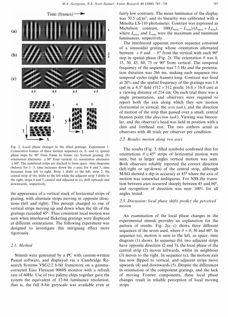
Fig. 2. Local phase changes in the tilted gratings. Experiment 1.Consecutive frames of three motion sequences (a, b, and c); spatialphase steps by 90° from frame to frame. (a) Vertical grating; (b)orientation alternates 930° from vertical; (c) orientation alternates960°. The numbered strips are stacked to form space–time diagrams(below); for 1–3, time increases down the y-axis; for 4 and 5, timeincreases from left to right. Strip 1 drifts to the left; strip 2, thecentral strip of (b), drifts to the left while the adjacent strip 3 drifts tothe right; strips 4 and 5, central and adjacent in (c), drift upwards anddownwards, respectively.

fairly low contrasts. The mean luminance of the displaywas 70.5 cd/m2, and its linearity was calibrated with aMinolta LS-110 photometer. Contrast was expressed asMichelson contrast, 100(Lmax−Lmin)/(Lmax+Lmin),where Lmax and Lmin were the maximum and minimumluminances, respectively.

The interleaved apparent motion sequence consistedof a sinusoidal grating whose orientation alternatedbetween +u and −u° from the vertical with each 90°step in spatial phase (Fig. 2). The orientation u was 0,15, 30, 45, 60, 75 or 90° from vertical. The temporalfrequency of the sequence was 7.5 Hz and the presenta-tion duration was 266 ms, making each sequence twotemporal cycles (eight frames) long. Contrast was fixedat 20% and the spatial frequency of the gratings was 1.0cpd in a 4.5° field (512×512 pixels; 16.8×16.8 cm) ata viewing distance of 214 cm. On each trial there was asingle presentation, and observers were required toreport both the axis along which they saw motion(horizontal or vertical; the axis task), and the directionof motion of the strip that passed over a small, centralfixation point (the direction task). Viewing was binocu-lar, and the observer’s head was held in position with achin and forehead rest. The two authors acted asobservers with 48 trials per observer per condition.

2.2. Results: motion along two axes

The results (Fig. 3, filled symbols) confirmed that fororientations u545° strips of horizontal motion wereseen, but at larger angles vertical motion was seen.Both observers reliably reported the correct direction(left/right or up/down) of the central strip, althoughMAG showed a dip in accuracy at 45° where the axis ofmotion was somewhat ambiguous. For NSS the transi-tion between axes occurred sharply between 45 and 60°,and recognition of direction was near 100% for allangles tested.

2.3. Discussion: local phase shifts predict the percei6edmotion

An examination of the local phase changes in theexperimental stimuli provides an explanation for thepattern of results. Fig. 2(a–c) shows three differentsequences of the seven used, where u=0, 30 and 60°. Insequence (a), motion is seen to the left, as space–timediagram (1) shows. In sequence (b), two adjacent stripshave opposite direction (2 and 3); the local phase of thecentral strip (2) moves leftwards, whilst its neighbour(3) moves to the right. In sequence (c), the motion axishas now flipped to vertical, and adjacent strips moveupwards (4) and downwards (5). Despite the differencesin orientation of the component gratings, and the lackof moving Fourier components, these local phasechanges result in reliable perception of local movingstrips.

the appearance of a vertical stack of horizontal strips ofgrating, with alternate strips moving in opposite direc-tions (left and right). This percept changed to one ofvertical strips moving up and down when the tilt of thegratings exceeded 45°. Thus consistent local motion wasseen when interleaved flickering gratings were displayedat different orientations. The following experiment wasdesigned to investigate this intriguing effect morerigorously.

2.1. Method

Stimuli were generated by a PC with custom-writtenPascal software, and displayed via a Cambridge Re-search Systems VSG2/2 8-bit framestore on a gamma-corrected Eizo Flexscan 9060S monitor with a refreshrate of 60Hz. Use of two palette chips together gave thesystem the equivalent of 12-bit luminance resolution;that is, the full 8-bit greyscale was available even at


Fig. 3. Strip direction and axis results. Experiment 1. Results for two subjects (NSS and MAG) for both the axis task (filled circles, solid line)and direction task (open squares, dashed line), expressed as % correct for the direction task (left hand ordinate), and as % judged horizontal forthe axis task (right hand ordinate). The x-axis shows the orientation u for each sequence.

The dip in direction performance for observer MAGat u=45° (Fig. 3) indicates that the direction task isconfounded by an uncertainty in the axis task at thisvalue. A dip was not observed for observer NSS be-cause there was a sharp transition in the axis taskbetween u=45 and 60°, and so no uncertainty waspresent for this observer. This transition from left/rightto up/down does not mean that there is no energy alongthe orthogonal axis; for all values 0BuB90° there isboth horizontal and vertical local motion present, as weshow below. The transition from horizontal to verticalmotion perception presumably reflects the relati6e 6isi-bility of these two motions.

A grating of spatial frequency f and orientation u hashorizontal and vertical periodicities (u, 6) where u=f cos u and 6= f sin u. In the Appendix we show that ifmotion perception is based on local phase shifts, thenthe sequences used here contain horizontally movingstrips whose height is 1/(4 6), one quarter of the verticalperiod (1/6). Informal observation confirmed that thiswas indeed the height of the perceived strips. Interest-ingly, the switching of orientations can also be de-scribed as having constant 6 with alternation between uand −u (see Fig. 4) and by an entirely similar argu-ment one can show that there are also vertical strips ofupward and downward phase shift whose width is 1/(4u).

In principle, then, there are two alternative interpre-tations for each of our sequences — horizontal orvertical strips of motion. However, when 05uB45°,6Bu, and the horizontal strips are wider than thevertical ones, but when 45B u590° 6\u and thevertical strips are wider than the horizontal. A likelyexplanation for the crossover from horizontal to verti-cal motion perception (Fig. 3) is that two mechanisms,orthogonally tuned, respond to the two axes of motion.We assume that the two mechanisms have peak sensi-

tivities on the u-axis and 6-axis, respectively (Fig. 4).Grating components close to the u-axis (uB45) willevoke a horizontal motion response more strongly thanvertical, and vice versa for u\45. Since there was littleor no evidence for ambiguity or transparency in theaxis task (Fig. 3) it seems likely that the strongerresponse suppresses the weaker — ‘winner takes all’. Itfollows that, in spatial terms, the wider strips determinethe perceived axis of motion. One might expect thecrossover point to be at u=45°, but experimentally thecrossover was between 45 and 60°. It may be thatextensive practice on horizontally moving stimuli cre-ated some bias in favour of the horizontalinterpretation.

We did not observe oblique motion. It might seemsurprising that the vertical and horizontal motions em-bedded in this animation do not sum to form obliquemovements. Alternate rows (and columns), however,have opposite directions of movement, and so the pat-tern of oblique movements obtained by summationwould form a checkerboard in which every small square

Fig. 4. Two orthogonal motion detectors. Experiment 1. (a) uB45°gives horizontal motion, and (b) u\45° gives vertical motion. Thegrey ovals show (a) vertically oriented detectors, (b) horizontallyoriented. Note that, as u varies, the stimuli follow a circular paththrough u–6 space, because grating spatial frequency was fixed[(u1

2+612)= (u2

2+622)=constant].


Fig. 5. The grating-plaid sequence. Experiment 2. Below: four framesof the grating-plaid motion sequence (phases 0, 90, 180, 270°; alter-nate frames of grating and plaid). Above: Fourier representation ofthe vertical grating (white dots) and the plaid components (blackdots). Both fall within the same vertical detector (light ovals), butonly the plaid components fall within the horizontal detector (darkovals).

tion sensitivity of the detectors the stimulus sequenceused here is problematic. Different detectors are re-cruited at large and small angles, and so there is no wayto test the responsiveness of the horizontal motiondetector when u\45. It was therefore necessary todevise a stimulus sequence that would anchor the mo-tion to the horizontal direction and test only onedetector.

3. Experiment 2: the grating-plaid sequence

To restrict motion to just one axis, we used thegrating-plaid sequence (Fig. 5). The critical feature ofthis sequence is that the alternate frames of verticalgrating prevent the mechanism for vertical motion(dark shaded ovals) from detecting anything other thanflicker, as this mechanism is sensitive only to the coun-terphasing plaid components. The mechanism for hori-zontal motion (light shaded ovals), on the other hand,is able to detect both the plaid and grating components,and can therefore produce motion signals by integrat-ing these two images over time. Initial observationsconfirmed that this sequence produced horizontal, butnot vertical, strips of apparent motion (see Fig. 6).

From Fig. 5 it can be seen that increasing the angle(u) of the plaid components from the vertical whilemaintaining constant horizontal periodicity (u) has theeffect of increasing the vertical spatial frequency (6).This means that, as before, the strips of motion arethinner with increasing u, but now the height of thestrips is 1/(2 6). At sufficiently high values of u, theplaid components will fall outside the detector (lightgrey ovals in Fig. 5) and motion perception will fail.The limiting value, umax, gives a measure of the orienta-tion range of that detector.

The height of the detector’s RF may also be inferredfrom the grating-plaid sequence. We assume that whenequal and opposite amounts of motion energy fallwithin the receptive field the response of that detectorwill be zero. It follows that when two oppositely mov-ing (but otherwise identical) strips exactly cover thedetector, no motion signal will arise (see Fig. 7b). Thisis not so if less than two strips fall on the detector (Fig.7a), in which case there is a predominant motion signalin one direction, but it remains so with more than twostrips (Fig. 7c). Thus at umax, the height of the strips inthe stimulus sequence should equal half the height ofthe motion detector. This strip height is the critical stripheight.

3.1. Method

Apparatus was similar to experiment 1. The inter-leaved grating-plaid sequence had a temporal frequencyof 7.5 Hz, and was viewed for 266 ms (two cycles). The

Fig. 6. Local phase shifts in the grating-plaid sequence. Experiment 2.Consecutive frames of two motion sequences; spatial phase steps by90° from frame to frame. (a) Vertical grating; (b) vertical gratingalternates with a plaid. Numbered strips are stacked to producespace–time diagrams in which time is increasing down the y-axis.Strip 1 drifts to the left, while strips 2 and 3 (adjacent in thegrating-plaid sequence) drift to the right and left, respectively.

had a direction orthogonal to its neighbours. Along thediagonals of the checkerboard, adjacent squares haveopposite directions which presumably cancel eachother, or lose out in the competition with the coherenthorizontal (or vertical) motion available in rows (orcolumns).

This is a reasonably satisfying account of an intrigu-ing motion phenomenon, but for revealing the orienta-


Fig. 7. Inferring the receptive field height. White rectangle representsthe receptive field (RF) of a motion detector; light and dark grey barsare leftward and rightward strips of the grating-plaid sequence. (a)Most of the RF is occupied by a rightward-moving strip, and thedetector signals rightward motion. (b) Equal areas of the RF areoccupied by rightward- and leftward-moving strips, yielding an am-biguous signal. (c) Similar to (b) but more strips occupy the RF. Thuswhen strip height decreases to the critical strip height (b) motionsignalling breaks down. RF height is given by twice the critical stripheight (but see text for exact definition of height H).

Both the fixation point and side cursors were displayedfor 250 ms before each trial. The contrast of the singlegratings was fixed at 20% but the plaid contrast variedacross sessions, taking values of 20, 40 or 80%. Thiswas to compensate for any possible attenuation of theplaid components due to their off-vertical orientationand higher spatial frequency [ f=(u2+62)]. Percentcorrect direction judgements were plotted against u andlimiting values umax were derived at 75% correct from alogistic curve fitted to the psychometric function data.

3.2. Results: motion recepti6e fields are 6ery short

The results for observer NSS (see Fig. 8, left) showthat the critical angle, umax at 75% correct, was greaterthan 80° at the lower spatial frequencies, decreasing toaround 60° at the highest spatial frequency tested. Thisindicates that motion mechanisms are sensitive over avery broad range of orientations. Note also that whenu=80° the radial spatial frequency ( f ) of the plaid’scomponents is 5.8 times higher (2.5 octaves higher)than the grating, showing that the motion detector cancombine information from components differing verywidely in both orientation and spatial frequency. Thekey factor is the coherence of local phase changes. Atall four spatial frequencies (u values) there was nosystematic effect of changing plaid contrast.

In general, 6/u= tan u, and so from the observedumax values we derive a corresponding 6max which is thespatial frequency of the strips themselves (not the SF ofthe content of the strips) at the point where motiondirections can just be resolved:

6max=u tan umax (1)

where u and 6 are the vertical and horizontal spatialfrequencies of the plaid, and umax is the critical plaidangle (see Fig. 5). If we assume that the vertical profileof the receptive field is Gaussian then its extent can berepresented as 2.5sy, the Gaussian equivalent width,which is the width of a rectangle that has the sameheight and area as a Gaussian with standard deviation

stimulus spatial frequencies were changed by adjustingthe viewing distance across sessions; the four viewingdistances (20, 71, 214 and 642 cm) gave horizontalspatial frequencies of 0.10, 0.33, 1.00 and 3.00 cpd forboth grating and plaid components. The horizontalperiodicity of all stimuli was 4.5 cycles/image. Observ-ers were required to indicate the direction of motion ofa central strip in a single interval, binary choice task.This centrally located strip varied in height accordingto the vertical spatial frequency (6) of the plaid ele-ments of the motion sequence, which varied acrosstrials within a single session. A central fixation pointwas provided and cursors on each side of the displayindicated the location and height of the central strip.

Fig. 8. Orientation range and RF height. Experiment 2. Orientation range in degrees (left) and RF height (H) in cycles (right) plotted againsthorizontal spatial frequency for one observer (NSS).


Table 1Experiment 2: spatial and temporal frequency, speed and perfor-mance for NSS expressed in six different waysa

10.1 30.33 u, cpd7.5 7.57.5 TF, Hz7.5

22.575 7.5 2.5 Speed, deg/s84 84 77 63 umax, °

4.33 5.893.14 6max, cpd0.950.160.53 0.12 0.08 Critical strip, deg0.130.42 0.09 0.07 sy, deg

0.18 0.410.08 H, cycles0.0850.45 11.0815.29 8.15 RF height, min arc

a Bottom row shows RF height estimated as 2 sy converted to minarc.

the results, summarized in Table 1, was the shortness ofthe receptive fields, which ranged from as little as 0.08cycles at 0.1 and 0.3 cpd, to 0.4 cycles (8 min arc) at 3.0cpd.

3.3. Discussion: extraneous cue to motion, and the stripuncertainty problem

The second observer (MAG) reported the existenceof an extraneous cue to direction in the grating-plaidsequence. An image-processing analysis of the grating-plaid sequence revealed that visual temporal integrationover consecutive frames gave rise to an extraneousstatic cue to the direction of motion of the central strip.The cue had the appearance of a stationary, spatiallyperiodic ‘wiggly’ distortion across the display in thevertical direction, with spatial frequency 6. The spatialphase of this distortion signalled the direction of mo-tion of the central strip. MAG’s data were thereforediscarded. The data from NSS, who did not notice thiseffect, were apparently unaffected by it.

The experiment was designed to reveal the orienta-tion range and receptive field height of 1st-order mo-tion detectors, but the decline in performance withdecreasing strip height that was used to estimate thesevalues could have been influenced by uncertainty as towhich strip was to be judged. Uncertainty over whichstrip was being marked by the cursors could makeperformance fall to chance prematurely. It is thereforepossible that the true receptive field height is evenshorter (and the orientation range wider) than ourestimates. Furthermore, if the filter were polar separa-ble in the u–6 domain, rather than Cartesian separable,then this would also result in an underestimation of thereceptive field height. The results must therefore beregarded as conservative estimates of these quantities.

4. Experiment 3: the moving strips sequence

To eliminate the artefactual cue described above, athird sequence was constructed by taking two driftinggratings, one moving to the left, the other to the right,and cutting both into horizontal strips of a givenheight. These strips were then stacked on top of oneanother, alternate strips coming from one or other ofthe two original gratings, to form the strips sequence(Fig. 9).

Comparison of Fig. 9 with Fig. 6 reveals that thelocal space–time diagrams of the grating-plaid andstrips sequences are very similar. In fact, by shifting therelative phases of the two original gratings, it is possibleto make a strips sequence that is practically indistin-guishable from the grating-plaid sequence. In Fig. 9b,the phases used for the two constituent gratings are

Fig. 9. Local phase in the strips stimuli. Experiment 3. Consecutiveframes of two motion sequences. (a) Vertical grating; the four frameshave phases 0, 90, 180 and 270°, reading from left to right; (b) isconstructed from two oppositely-drifting gratings with phases 0, 90,180 and 270°, and 270, 180, 90 and 0°, which are cut up horizontallyand reassembled as alternate strips. The numbered slices are stackedto produce space–time diagrams in which time is increasing down they-axis. Strip 1 drifts to the left, while 2 and 3, adjacent strips insequence (b), drift to the left and right, respectively.

sy. The angle subtended by two strips is one verticalperiod of the plaid (1/6), and thus sy can be estimatedfrom the assumption outlined above that the equivalentheight of the Gaussian equals two critical strip heights:

2.5 sy=16max

(2)

Combining Eqs. (1) and (2) we get:

sy=4

10 u tan umax

(3)

Anderson and Burr (1991) expressed their RF heightestimates (H) in cycles of the tested spatial frequency,as H=2 u sy, and so for direct comparison we haveexpressed our results the same way. Receptive fieldheight (H, in cycles) is plotted against horizontal spatialfrequency (u) in Fig. 8, right. H was not constant, butincreased with spatial frequency. A striking feature of


0–90–180–270° and 270–180–90–0°. This arrange-ment ensures that adjacent strips are always 90° out ofphase. An image-processing analysis of the new se-quence confirmed that it did not contain a static cuelike that found in the grating-plaid sequence.

4.1. Method

The apparatus and procedure were the same as ex-periment 2. The only difference was that the alternatingframes of grating and plaid were replaced by consecu-tive frames of the strips sequence, and that all frames ofthe sequence were displayed at 20% contrast. The twoauthors and a naive volunteer acted as observers. Criti-cal strip heights (at 75% correct) were estimated fromthe fitted psychometric functions, and converted intoRF height estimates (H) as before.

4.2. Results: confirmation of the grating-plaid data

Fig. 10 shows the receptive field height estimates (H,in cycles) for all three observers, along with the data forobserver NSS from experiment 2 (the grating-plaidsequence). Although there were slight variations acrossobservers, the pattern of results was similar. The resultsfrom the strips sequence for NSS were encouraginglysimilar to the data from the grating-plaid sequence,confirming that the extraneous cue in experiment 2 hadnot affected NSS’s data. As with the grating-plaidsequence, the most striking feature of the results is theshortness of the estimated receptive field heights, vary-ing from around 0.1 to 0.4 cycles of the grating periodover the spatial frequency range tested (0.1–3.0 cpd).The orientation range implied by these receptive fieldheights is extremely wide.

RF height estimates for observer NSS showed aslight but consistent decrease at each spatial frequency

in experiment 3, compared with experiment 2. This maybe related to the greater sharpness of the motionboundaries in the strips sequence, compared with thegrating-plaid sequence.

5. Experiment 4: controlling for contrast and temporalfrequency

In experiment 2, the grating frames had 20% contrastwhile the contrast of the plaid frames was 20, 40 or80%; the level of plaid contrast had little or no effectupon direction discrimination performance. In experi-ment 3 the strips sequence was displayed at 20% con-trast only. However, it is possible that performancemight improve with increasing contrast because moreenergy is put into the motion mechanism. The criticalstrip height might decrease, and the orientation rangewould increase. Such contrast dependence would under-mine our claim to be measuring RF height. Anotherpotentially important variable is temporal frequency:the height estimates in experiments 2 and 3 were ob-tained at 7.5 Hz drift rate. It might be that larger RFsare recruited at higher speeds, in which case our esti-mates would increase with temporal frequency.

5.1. Method

The methods were as experiment 3, except that spa-tial frequency was 1.0 cpd in all cases, and acrossdifferent sessions either (i) the contrast of the stripssequence was varied (5, 10, 20, 40 or 80%) at fixedtemporal frequency (7.5 Hz), or (ii) the temporal fre-quency of the stimulus sequence was varied (15.0, 7.5,3.75 or 1.875 Hz) at fixed contrast (20%). The formercondition was the contrast condition, the latter thetemporal frequency condition. The duration of the dis-play was constant at 266ms in all cases, and in condi-tion (ii) this meant that only half a temporal cycle wasshown at 1.875 Hz. To prevent the motion sequencefrom appearing ‘jerky’ (undersampled), 45° phase shiftsbetween consecutive frames were used at 1.875 Hzinstead of the 90° phase shifts employed at the othertemporal frequencies. Both authors acted as observersin the contrast condition (i), NSS in the temporalfrequency condition (ii).

5.2. Results

(i) RF height estimates (H, in cycles) for the twoobservers (MAG and NSS) in the contrast conditionare shown in Fig. 11(a). At contrasts below 20% Hincreased markedly, whereas at and above 20% contrastH was fairly constant. (ii) There was no systematicvariation in critical strip height across temporal fre-quency (Fig. 11b), implying that the value of 7.5 Hzused in the earlier experiments was appropriate.

Fig. 10. Grating-plaid and strips sequences compared. Results forthree observers (AKS, MAG and NSS) for experiment 3 (the stripssequence), and one observer (NSS) for experiment 2 (the grating-plaidsequence). Receptive field height H in cycles is plotted against hori-zontal spatial frequency on log–log axes.


Fig. 11. The effect of contrast and temporal frequency. (A) Experi-ment 4(i). Receptive field height H in cycles plotted against thecontrast of the strips sequence for two observers (MAG and NSS) ata spatial frequency of 1.00 cpd. (B) Experiment 4(ii). Directiondiscrimination performance against strip height (in pixels) for NSS atfour speeds (temporal frequencies) at 1 cpd, 20% contrast. 1 pixel=0.53 min arc. Threshold strip height was about 6 min arc at allspeeds.

and 3 (Fig. 10) are representative estimates. Since criti-cal strip height reached its asymptotic level near 20%contrast, this finding validates the results from experi-ment 3 carried out at 20% contrast. RF height esti-mates would not have been much smaller at highercontrasts. This suggests that a structural limit, im-posed by the receptive field height itself, has beenreached at about 20–40% contrast. At lower contrastsreduction of signal:noise ratio may cause performanceto be worse than this structural limit.

Variation of temporal frequency had no systematiceffect on receptive field height estimates, at least up to15Hz as tested here. Thus spatial resolution for shear-ing motion is determined by local spatial frequency(u), not by speed of movement. This conclusion con-trasts with the findings of Koenderink et al. (1985)who found that the strip width required for spatialsegregation of strips of random dots moving in oppo-site directions increased markedly with speed, beingabout 8 min arc at 1°/s but 100 min arc at 10°/s. Thedifference may be largely due to differences in the typeof motion: shearing motion (along the strips) in ourexperiments versus expansive/compressive motion(across the strips) in the Koenderink study. As Koen-derink et al. point out, the segregation limit in theirexperiment was probably temporal rather than spatial:the dots had to spend about 70–100 ms traversing onestrip in order for the strips to be segregated. In ananalogous study using shearing motion of drifting ran-dom dots, Nakayama and Silverman (1984); their Fig.2) found that strips of motion only 13 min arc highcould just be resolved at 16°/s (Nakayama & Silver-man, 1984) which is much more in line with our find-ings.

6. General discussion

Fig. 12 shows a summary of the average RF heightestimates from experiments 2 and 3 for observer NSS,along with those of Anderson and Burr (1991) whoused a spatial summation technique to measure boththe width and height of motion receptive fields atthreshold. These authors published similar results frommasking experiments (Anderson & Burr, 1987, 1989,1991; Anderson, Burr & Morrone, 1991), andconfirmed that the RF size (in cycles) increases withincreasing spatial frequency. They also showed that theheights and widths of the receptive field envelopes wereequal. There is excellent agreement between Andersonand Burr’s (1991) results and our own, despite the verydifferent methods and theoretical assumptions used. Atall spatial frequencies the estimated receptive fieldheight is a small fraction of one spatial period. Theheights range from 0.08 cycles at 0.1 cpd to 0.38 cyclesat 3.0 cpd, corresponding to orientation ranges (in the

Fig. 12. RF height estimates. Averaged results for one subject (NSS)from experiments 2 and 3 (grating-plaid and strips sequences), com-pared with data from Anderson and Burr (1991). RF height in cyclesis plotted against horizontal spatial frequency.

5.3. Discussion: pre6ious parameter choices justified

The results from these two control experiments indi-cate that the values of RF height from experiments 2


plaid experiment) from about 984 to 965°,respectively.

6.1. The Gaussian deri6ati6e model

Do the estimates given above for RF height andorientation range correspond to plausible space–timefilters in motion analysis? To begin to answer thisquestion we consider a simple, general model for mo-tion filtering. Direction-selective linear filters have re-ceptive fields that are oriented in space–time (Adelson& Bergen, 1985) and it is well known that such fieldscan be formed by linear combination of pairs of RFsthat are 90° out of phase with each other in space andtime. This approach gives a good account of direction-selective simple cells (McLean & Palmer, 1989) andcomplex cells (Emerson, Bergen & Adelson, 1992) inthe primary visual cortex. An analytically tractableform for this kind of model is based on Gaussianderivatives (GDs) in space and time (Young, 1985;Adelson & Bergen, 1986; Johnston, McOwan & Bux-ton, 1992; Young & Lesperance, 1993). Thus if G(x, y,t) is a Gaussian function of space and time then Gx andGt (where subscripts denote partial differentiation withrespect to a given variable) are suitable subunits thatform an oriented space–time receptive field (M1) whenadded together: M1=Gx+Gt. Differentiating againwith respect to x gives us M2=Gxx+Gxt, which formsa direction-selective filter whose SF bandwidth is nar-rower than that of M1. See Bruce, Green andGeorgeson (1996) for illustration (their Fig. 8.7).Clearly, differentiating m times with respect to x candefine a family of filters Mm (m=1,2,3,4, …). M1 andM2 are odd and even filters in space–time and can beused as elements of the Adelson–Bergen energy modelto encode velocity exactly. There is an equivalencebetween this version of the energy model and at leastone form of the multichannel gradient model (Adelson& Bergen, 1986; Johnston et al., 1992; Bruce et al.,1996).

We now derive the spatio-temporal frequency re-sponse of Mm in order to see how such filters wouldrespond to the grating-plaid sequence of experiment 2.Since motion filters are not space–time separable, the2-D spatial frequency response depends on temporalfrequency, and the equations must be developed in 3-D(space–time) not 2-D space alone. Thus we define:

Mm(x, y, t)=(mG(xm +

(mG(xm−1(t

(4)

where G(x, y, t) is a Gaussian function with standarddeviations sx, sy, st. The Fourier transform F(u, 6, w)of G(x, y, t) is:

F(u, 6, w)=exp[−2p2(u2 sx2 +62 sy

2+w2 s t2)] (5)

Differentiation with respect to x or t multiplies thetransform by 2 p i uor 2 p i w, respectively. Hence theFourier transform (Fm) of Mm is:

Fm(u, 6, w)= (2 p i )m um−1(u+w)F(u, 6, w) (6)

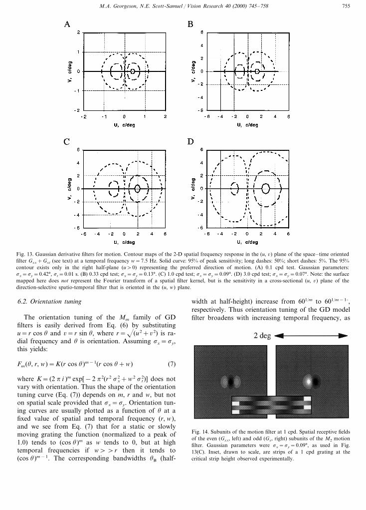
Fig. 13 shows iso-sensitivity contours of F2(u, 6, w) inthe (u, 6) plane for w=7.5 Hz, plotted using the valuesof sy from Table 1, and assuming sx=sy, st=0.01 s.These plots give an idea of the 2-D range of spatialfrequencies that could be combined by the second-derivative based motion filter (Gxx+Gxt) in order toextract the motion of strips in the grating-plaid experi-ment. Positive u values represent motion in the pre-ferred direction, negative u values are the non-preferreddirection. The outermost contour in each plot is thelocus of spatial frequencies (u, 6) for which the filter has5% of its peak sensitivity at w=7.5 Hz. We note that ineach case the range of plaid frequencies (6max) thatsupported perception of moving strips would be nearlyaccounted for if the limit of performance was imposedby the 5% sensitivity contour.

For example, our empirical estimate of sy was 0.09°for a grating of 1 cpd; Fig. 13(C) shows that the M2

filter defined by this spatial scale has a peak sensitivityat u=1.9 cpd, and at u=1 cpd the 5% contour extendsout to 6=4.0 cpd. This compares well with our experi-mental 6max of 4.33 cpd (Table 1). Across the four testspatial frequencies (0.1, 0.33, 1, 3 cpd) the 6max valuesfrom Table 1 are 0.95, 3.1, 4.3, 5.9 cpd, compared with6=0.78, 2.5, 4.0, 5.7 cpd at the 5% limit derived fromFig. 13(A–D). The agreement here is fairly good, butthe argument depends on the assumption that humanperformance fails when the filter’s response to one plaidcomponent falls to about 5% of its response to thevertical grating (given that the SF of the vertical gratinglies near the peak of the filter). Bearing in mind thatthere are two plaid components, the limiting response(to the plaid) should be about 10% of the response tothe optimal grating. We have independent evidence thatthis limit is about right. In a separate study (Georgeson& Scott-Samuel, 1999) the motion sequence (cf. Fig. 1)consisted simply of interleaved 1 cpd vertical gratingsof two different contrasts. Recognition of direction fellto chance when the contrast of one grating fell belowabout 10% of the other grating, irrespective of absolutecontrast. This would correspond to a 5% response limitfor each of the plaid’s components.

In summary, then, the 2-D spatial bandwidth of thesecond-derivative motion filter (M2) based upon a cir-cular Gaussian (where sx=sy) appears well suited toaccount for our results on spatial resolution of strips ofmotion. The similarity between our RF height estimatesand those of Anderson and Burr (1991) obtained byvery different means lends strong support to this con-clusion. Fig. 14 illustrates the short, stubby receptivefields of the M2 filter that are implied by this analysis.


Fig. 13. Gaussian derivative filters for motion. Contour maps of the 2-D spatial frequency response in the (u, 6) plane of the space–time orientedfilter Gxx+Gxt (see text) at a temporal frequency w=7.5 Hz. Solid curve: 95% of peak sensitivity; long dashes: 50%; short dashes: 5%. The 95%contour exists only in the right half-plane (u\0) representing the preferred direction of motion. (A) 0.1 cpd test. Gaussian parameters:sx=sy=0.42°, st=0.01 s. (B) 0.33 cpd test; sx=sy=0.13°. (C) 1.0 cpd test; sx=sy=0.09°. (D) 3.0 cpd test; sx=sy=0.07°. Note: the surfacemapped here does not represent the Fourier transform of a spatial filter kernel, but is the sensitivity in a cross-sectional (u, 6) plane of thedirection-selective spatio-temporal filter that is oriented in the (u, w) plane.

6.2. Orientation tuning

The orientation tuning of the Mm family of GDfilters is easily derived from Eq. (6) by substitutingu=r cos u and 6=r sin u, where r=(u2+62) is ra-dial frequency and u is orientation. Assuming sx=sy,this yields:

Fm(u, r, w)=K(r cos u)m−1(r cos u+w) (7)

where K= (2 p i )m exp[−2 p2(r2 sx2 +w2 s t

2)] does notvary with orientation. Thus the shape of the orientationtuning curve (Eq. (7)) depends on m, r and w, but noton spatial scale provided that sx=sy. Orientation tun-ing curves are usually plotted as a function of u at afixed value of spatial and temporal frequency (r, w),and we see from Eq. (7) that for a static or slowlymoving grating the function (normalized to a peak of1.0) tends to (cos u)m as w tends to 0, but at hightemporal frequencies if w\\r then it tends to(cos u)m−1. The corresponding bandwidths uB (half-

width at half-height) increase from 601/m to 601/m−1$,respectively. Thus orientation tuning of the GD modelfilter broadens with increasing temporal frequency, as

Fig. 14. Subunits of the motion filter at 1 cpd. Spatial receptive fieldsof the even (Gxx, left) and odd (Gx, right) subunits of the M2 motionfilter. Gaussian parameters were sx=sy=0.09°, as used in Fig.13(C). Inset, drawn to scale, are strips of a 1 cpd grating at thecritical strip height observed experimentally.


observed in adaptation experiments (Snowden, 1992)and masking experiments (Anderson et al., 1991). Thebroadening of model tuning is greatest for m=1 wherethe filter has a half-bandwidth uB of 60° when w=0, butbecomes completely non-oriented when temporal fre-quency is high. This correctly reflects the behaviour ofadaptation and masking at very low spatial frequencies(0.1–0.2 cpd) (Kelly & Burbeck, 1987; Snowden, 1992).When m=2, uB increases from 45 to 60° with increasingtemporal frequency; when m=4 it shifts from 32.8 to37.5°, and when m=6 it shifts from 27.0 to 29.5°. Thusincreasing the derivative number (m) mirrors the twoeffects of adaptation observed by Snowden: with in-creasing spatial frequency the orientation bandwidthsdecrease, and the effect of temporal frequency on band-width progressively disappears. Experimental estimatesof spatial frequency bandwidth (in octaves) also becomenarrower with increasing peak SF (Wilson, Levi, Maf-fei, Rovamo & De Valois, 1990) and so an attractiveway to model this important cluster of results in theGaussian derivative (GD) framework (Eq. (4)) is tosuppose that for low SF channels m=1 or 2, but athigher SFs m increases progressively to around 4–6 (seeBruce et al., 1996, their Fig. 5.8). Accompanying theincrease in m is a decrease in the spatial scale (sx, sy).

Many details remain to be worked out, partly becausethe available data on bandwidths are fragmentary, andit also appears that Snowden’s (1992) orientation band-widths are systematically smaller than one would expectfrom the GD model with a circular base Gaussian (i.e.sx=sy). Physiological data indicate that cells in visualcortex have quite a range of bandwidths at each centrefrequency (De Valois, Albrecht & Thorell, 1982), and soit is possible that different psychophysical tasks tap intodifferent subsets of cells. For example, the tuning re-vealed in adaptation experiments might reflect the morenarrowly tuned cells at each spatial frequency, while ourexperiments may reveal the shortest RFs and hencemore broadly tuned cells. Although Fig. 13 illustratesthe SF tuning surfaces for m=2, our results are consis-tent with the idea outlined above that the derivativeorder m increases with the peak SF of the filter. Settingm=3 gave good predicted values of 6max at 3 cpd, butnot at 0.1 or 0.33 cpd where the narrowing of band-width (in going from m=2 to m=3) made the filterstoo insensitive at low SFs.

6.3. Off-frequency looking?

Our experiments yield fairly direct estimates of theRF length factor (sy), but not the width factor (sx). Inanalyzing the GD model we have supposed that sx=sy,and shown that this model is consistent with our data.What happens if sxBBsy? This creates a filter with amore conventional, elongated but narrower RF, and ahigher peak SF with narrower orientation tuning at the

peak SF. However, it turns out that in the 2-D fre-quency domain (as Fig. 13) the ‘skirts’ of the M2 filterresponse can be quite broad, and that an oriented filtercentred at say 4 or 6 cpd could have sufficiently broadorientation bandwidth at 6=1 cpd to be consistent withour 1 cpd data, though the sensitivity to the gratingcomponent would be low. Such use of an effective, butless sensitive channel is known as ‘off-frequency look-ing’. It could play a part in our experiments, wherecontrast is well above threshold. However, off-fre-quency looking is unlikely to contribute much to perfor-mance at contrast threshold, and so the similaritybetween our results and those of Anderson and Burr(1991) obtained at threshold (Fig. 12) strengthens theargument that short, stubby receptive fields for motiondo exist in human vision (Fig. 14) (though for a differ-ent view, see Watson and Turano (1995)).

6.4. Implications for motion integration in plaids

The very broad orientation selectivity implied bythese short RF heights suggests a surprisingly simplesolution to the aperture problem for coherent plaidmotion. Such broadband detectors would passively inte-grate plaid components over a wide range of orienta-tions, and hence respond to the movement of localstructure (local phase shifts) in the plaid, as we haveshown. Active schemes for combining the motion com-ponents of a plaid pre-suppose that the components areinitially processed separately in narrowband filters. Ourresults suggest that this may not be true in general, andso more explicit schemes for combination such as theintersection of constraints (IOC) rule (Adelson &Movshon, 1982) or vector–sum rule (Wilson, Ferrera &Yo, 1992) might be unnecessary in many cases. Perhapswe should not be asking how component motions arecombined, but how are they ever segregated? Recentmodels (Wilson & Kim, 1994) and experiments (Smith,Curran & Braddick, 1999) have begun to address thisissue.

Acknowledgements

This work was supported by a BBSRC studentship toNSS, and by BBSRC grant GR/G63582 to MAG. Partsof this work have previously been presented in abstractform (Georgeson & Scott-Samuel, 1994; Scott-Samuel &Georgeson, 1996).

Appendix A

For experiment 1, the height of the strips seen in thestimulus sequence can be derived as follows. A sinu-soidal grating may be written as:


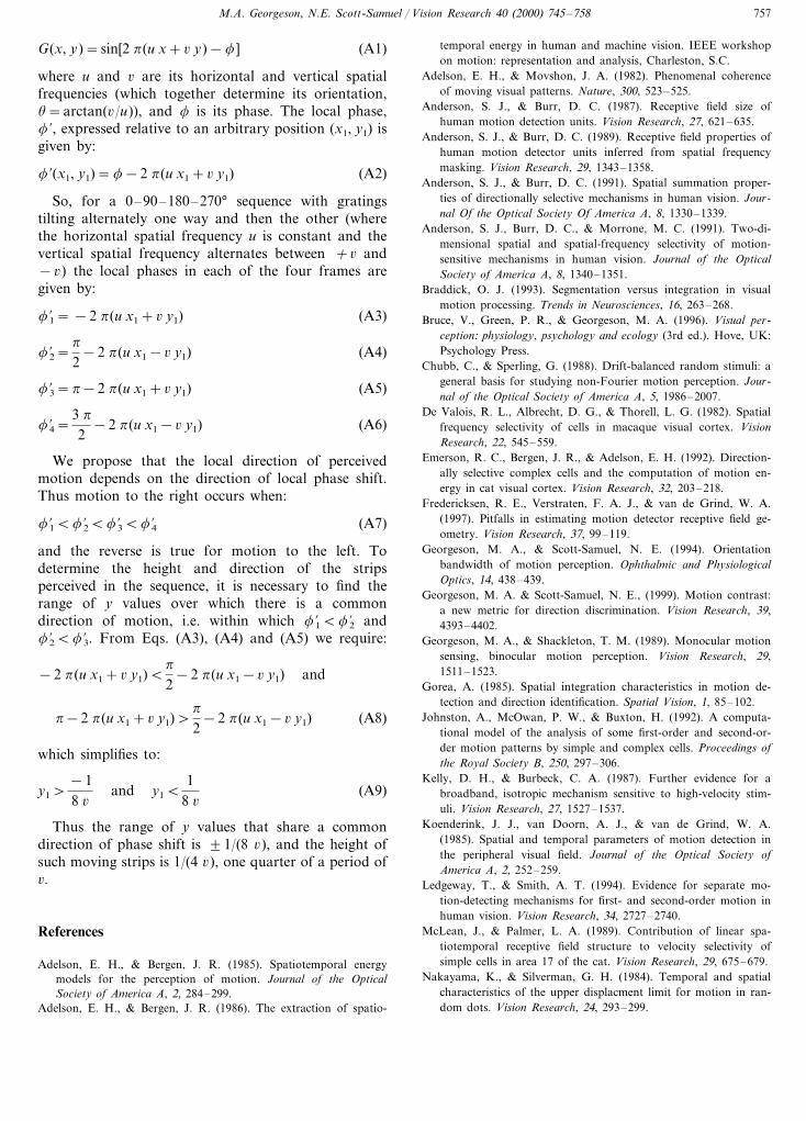
G(x, y)=sin[2 p(u x+6 y)−f ] (A1)

where u and 6 are its horizontal and vertical spatialfrequencies (which together determine its orientation,u=arctan(6/u)), and f is its phase. The local phase,f %, expressed relative to an arbitrary position (x1, y1) isgiven by:

f %(x1, y1)=f−2 p(u x1+6 y1) (A2)

So, for a 0–90–180–270° sequence with gratingstilting alternately one way and then the other (wherethe horizontal spatial frequency u is constant and thevertical spatial frequency alternates between +6 and−6) the local phases in each of the four frames aregiven by:

f %1= −2 p(u x1+6 y1) (A3)

f %2=p

2−2 p(u x1−6 y1) (A4)

f %3=p−2 p(u x1+6 y1) (A5)

f %4=3 p

2−2 p(u x1−6 y1) (A6)

We propose that the local direction of perceivedmotion depends on the direction of local phase shift.Thus motion to the right occurs when:

f %1Bf %2Bf %3Bf %4 (A7)

and the reverse is true for motion to the left. Todetermine the height and direction of the stripsperceived in the sequence, it is necessary to find therange of y values over which there is a commondirection of motion, i.e. within which f1%Bf2% andf2%Bf3% . From Eqs. (A3), (A4) and (A5) we require:

−2 p(u x1+6 y1)Bp

2−2 p(u x1−6 y1) and

p−2 p(u x1+6 y1)\p

2−2 p(u x1−6 y1) (A8)

which simplifies to:

y1\−18 6

and y1B1

8 6(A9)

Thus the range of y values that share a commondirection of phase shift is 91/(8 6), and the height ofsuch moving strips is 1/(4 6), one quarter of a period of6.

References

Adelson, E. H., & Bergen, J. R. (1985). Spatiotemporal energymodels for the perception of motion. Journal of the OpticalSociety of America A, 2, 284–299.

Adelson, E. H., & Bergen, J. R. (1986). The extraction of spatio-

temporal energy in human and machine vision. IEEE workshopon motion: representation and analysis, Charleston, S.C.

Adelson, E. H., & Movshon, J. A. (1982). Phenomenal coherenceof moving visual patterns. Nature, 300, 523–525.

Anderson, S. J., & Burr, D. C. (1987). Receptive field size ofhuman motion detection units. Vision Research, 27, 621–635.

Anderson, S. J., & Burr, D. C. (1989). Receptive field properties ofhuman motion detector units inferred from spatial frequencymasking. Vision Research, 29, 1343–1358.

Anderson, S. J., & Burr, D. C. (1991). Spatial summation proper-ties of directionally selective mechanisms in human vision. Jour-nal Of the Optical Society Of America A, 8, 1330–1339.

Anderson, S. J., Burr, D. C., & Morrone, M. C. (1991). Two-di-mensional spatial and spatial-frequency selectivity of motion-sensitive mechanisms in human vision. Journal of the OpticalSociety of America A, 8, 1340–1351.

Braddick, O. J. (1993). Segmentation versus integration in visualmotion processing. Trends in Neurosciences, 16, 263–268.

Bruce, V., Green, P. R., & Georgeson, M. A. (1996). Visual per-ception: physiology, psychology and ecology (3rd ed.). Hove, UK:Psychology Press.

Chubb, C., & Sperling, G. (1988). Drift-balanced random stimuli: ageneral basis for studying non-Fourier motion perception. Jour-nal of the Optical Society of America A, 5, 1986–2007.

De Valois, R. L., Albrecht, D. G., & Thorell, L. G. (1982). Spatialfrequency selectivity of cells in macaque visual cortex. VisionResearch, 22, 545–559.

Emerson, R. C., Bergen, J. R., & Adelson, E. H. (1992). Direction-ally selective complex cells and the computation of motion en-ergy in cat visual cortex. Vision Research, 32, 203–218.

Fredericksen, R. E., Verstraten, F. A. J., & van de Grind, W. A.(1997). Pitfalls in estimating motion detector receptive field ge-ometry. Vision Research, 37, 99–119.

Georgeson, M. A., & Scott-Samuel, N. E. (1994). Orientationbandwidth of motion perception. Ophthalmic and PhysiologicalOptics, 14, 438–439.

Georgeson, M. A. & Scott-Samuel, N. E., (1999). Motion contrast:a new metric for direction discrimination. Vision Research, 39,4393–4402.

Georgeson, M. A., & Shackleton, T. M. (1989). Monocular motionsensing, binocular motion perception. Vision Research, 29,1511–1523.

Gorea, A. (1985). Spatial integration characteristics in motion de-tection and direction identification. Spatial Vision, 1, 85–102.

Johnston, A., McOwan, P. W., & Buxton, H. (1992). A computa-tional model of the analysis of some first-order and second-or-der motion patterns by simple and complex cells. Proceedings ofthe Royal Society B, 250, 297–306.

Kelly, D. H., & Burbeck, C. A. (1987). Further evidence for abroadband, isotropic mechanism sensitive to high-velocity stim-uli. Vision Research, 27, 1527–1537.

Koenderink, J. J., van Doorn, A. J., & van de Grind, W. A.(1985). Spatial and temporal parameters of motion detection inthe peripheral visual field. Journal of the Optical Society ofAmerica A, 2, 252–259.

Ledgeway, T., & Smith, A. T. (1994). Evidence for separate mo-tion-detecting mechanisms for first- and second-order motion inhuman vision. Vision Research, 34, 2727–2740.

McLean, J., & Palmer, L. A. (1989). Contribution of linear spa-tiotemporal receptive field structure to velocity selectivity ofsimple cells in area 17 of the cat. Vision Research, 29, 675–679.

Nakayama, K., & Silverman, G. H. (1984). Temporal and spatialcharacteristics of the upper displacment limit for motion in ran-dom dots. Vision Research, 24, 293–299.


Scott-Samuel, N. E., & Georgeson, M. A. (1996). Receptive-field lengthof motion sensors in human vision. Perception (suppl.), 25, 125.

Scott-Samuel, N. E., & Georgeson, M. A. (1999). Does early non-lin-earity account for second-order motion? Vision Research, 39,2853–2865.

Shadlen, M., & Carney, T. (1986). Mechanisms of motion perceptionrevealed by a new cyclopean illusion. Science, 232, 95–97.

Smith, A. T., Curran, W., & Braddick, O. J. (1999). What motiondistributions yield global transparency and spatial segmentation?Vision Research, 39, 1121–1132.

Snowden, R. J. (1992). Orientation bandwidth: the effect of spatial andtemporal frequency. Vision Research, 32, 1965–1974.

van den Berg, A. V., van de Grind, W. A., & van Doorn, A. J. (1990).Motion detection in the presence of local orientation changes.Journal of the Optical Society of America A, 7, 933–939.

Watson, A. B., & Turano, K. (1995). The optimal motion stimulus.Vision Research, 35, 325–336.

Wilson, H. R., Ferrera, V. P., & Yo, C. (1992). A psychophysicallymotivated model for two-dimensional motion perception. VisualNeuroscience, 9, 79–97.

Wilson, H. R., & Kim, J. (1994). A model for motion coherenceand transparency. Visual Neuroscience, 11, 1205–1220.

Wilson, H. R., Levi, D. M., Maffei, L., Rovamo, J., & De Valois,R. L. (1990). The perception of form: retina to striate cortex.In L. Spillman, & J. S. Werner, Visual perception: the neuro-physiological foundations (pp. 231–272). London: AcademicPress.

Young, R. A. (1985). The Gaussian derivative theory of spatialvision: analysis of cortical cell receptive field line-weightingprofiles. Warren, MI: General Motors Research Labs. GMR-4920.

Young, R. A., & Lesperance, R. M. (1993). A physiological modelof motion analysis for machine vision. Warren, MI: GeneralMotors Research Labs. GMR-7878.

.

spatial resolution and receptive ﬁeld ... -...

Documents