Spatial Filtering

Background

Filter term in “Digital image processing” is referred to the subimageThere are others term to call subimage such as mask, kernel, template, or windowThe value in a filter subimage are referred as coefficients, rather than pixels.

Basics of Spatial Filtering

The concept of filtering has its roots in the use of the Fourier transform for signal processing in the so-called frequency domain.Spatial filtering term is the filtering operations that are performed directly on the pixels of an image

Mechanics of spatial filtering

The process consists simply of moving the filter mask from point to point in an image.At each point (x,y) the response of the filter at that point is calculated using a predefined relationship

Linear spatial filtering

f(x-1,y-1)f(x-1,y)f(x-1,y+1)

f(x,y-1)f(x,y)f(x,y+1)

f(x+1,y-1)f(x+1,y)f(x+1,y+1) w(-1,-1) w(-1,0) w(-1,1)

w(0,-1) w(0,0) w(0,1)

w(1,-1) w(1,0) w(1,1)

The result is the sum of products of the mask coefficients with the corresponding pixels directly under the mask

Pixels of image

Mask coefficients

w(-1,-1) w(-1,0) w(-1,1)

w(0,-1) w(0,0) w(0,1)

w(1,-1) w(1,0) w(1,1)

)1,1()1,1(),1()0,1()1,1()1,1(

)1,()1,0(),()0,0()1,()1,0(

)1,1()1,1(),1()0,1()1,1()1,1(

yxfwyxfwyxfw

yxfwyxfwyxfw

yxfwyxfwyxfw),( yxf

Note: Linear filtering

The coefficient w(0,0) coincides with image value f(x,y), indicating that the mask is centered at (x,y) when the computation of sum of products takes place.For a mask of size mxn, we assume that m-2a+1 and n=2b+1, where a and b are nonnegative integer. Then m and n are odd.

Linear filtering

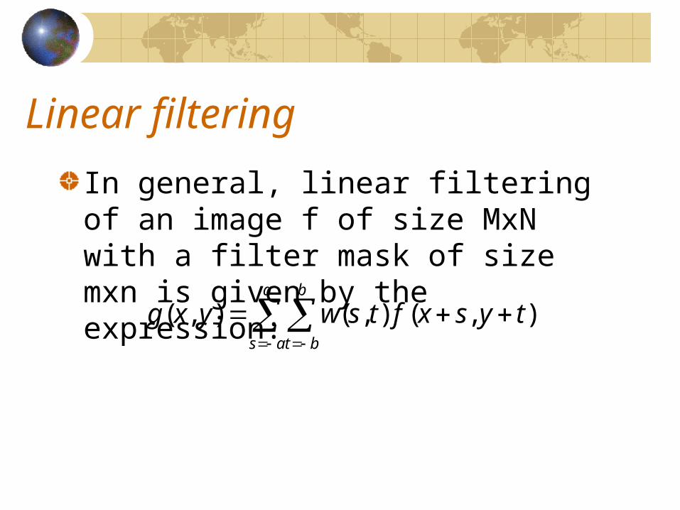
In general, linear filtering of an image f of size MxN with a filter mask of size mxn is given by the expression:

a

as

b

bt

tysxftswyxg ),(),(),(

Discussion

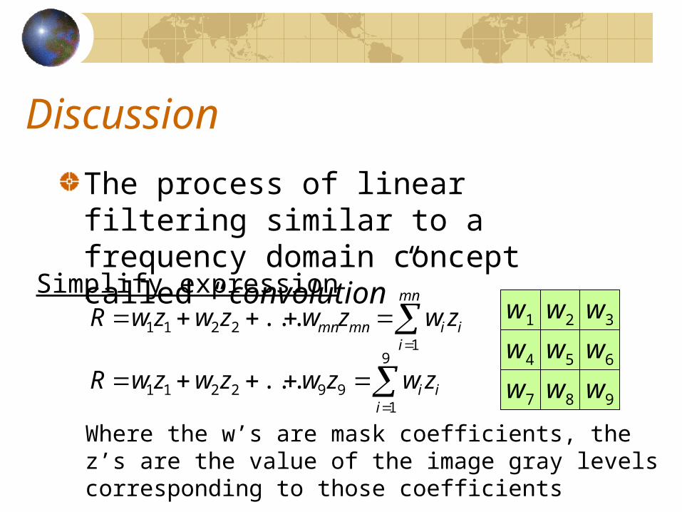
The process of linear filtering similar to a frequency domain concept called “convolution”

mn

iiimnmn zwzwzwzwR

12211 ...

9

1992211 ...

iii zwzwzwzwR

Simplify expressionw1 w2 w3

w4 w5 w6

w7 w8 w9

Where the w’s are mask coefficients, the z’s are the value of the image gray levels corresponding to those coefficients

Nonlinear spatial filtering

Nonlinear spatial filters also operate on neighborhoods, and the mechanics of sliding a mask past an image are the same as was just outlined.The filtering operation is based conditionally on the values of the pixels in the neighborhood under consideration

Smoothing Spatial Filters

Smoothing filters are used for blurring and for noise reduction.

– Blurring is used in preprocessing steps, such as removal of small details from an image prior to object extraction, and bridging of small gaps in lines or curves

– Noise reduction can be accomplished by blurring

Type of smoothing filtering

There are 2 way of smoothing spatial filters

Smoothing Linear FiltersOrder-Statistics Filters

Smoothing Linear Filters

Linear spatial filter is simply the average of the pixels contained in the neighborhood of the filter mask.Sometimes called “averaging filters”.The idea is replacing the value of every pixel in an image by the average of the gray levels in the neighborhood defined by the filter mask.

Two 3x3 Smoothing Linear Filters

1 1 1

1 1 1

1 1 1

1 2 1

2 4 2

1 2 1

9

1 16

1

Standard average Weighted average

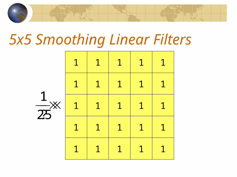
5x5 Smoothing Linear Filters

1 1 1

1 1 1

1 1 1

1

1

1

1

1

1

1 1 1 1 1

1 1 1 1 1

?

1

25

1

Smoothing Linear Filters

The general implementation for filtering an MxN image with a weighted averaging filter of size mxn is given by the expression

a

as

b

bt

a

as

b

bt

tsw

tysxftswyxg

),(

),(),(),(

Result of Smoothing Linear Filters

[3x3] [5x5] [7x7]

Original Image

Order-Statistics Filters

Order-statistics filters are nonlinear spatial filters whose response is based on ordering (ranking) the pixels contained in the image area encompassed by the filter, and then replacing the value of the center pixel with the value determined by the ranking result.Best-known “median filter”

Process of Median filter

Corp region of neighborhoodSort the values of the pixel in our regionIn the MxN mask the median is MxN div 2 +1

10 15 20

20 100 20

20 20 25

10, 15, 20, 20, 20, 20, 20, 25, 100

5th

Result of median filter

Noise from Glass effect Remove noise by median filter

Homework

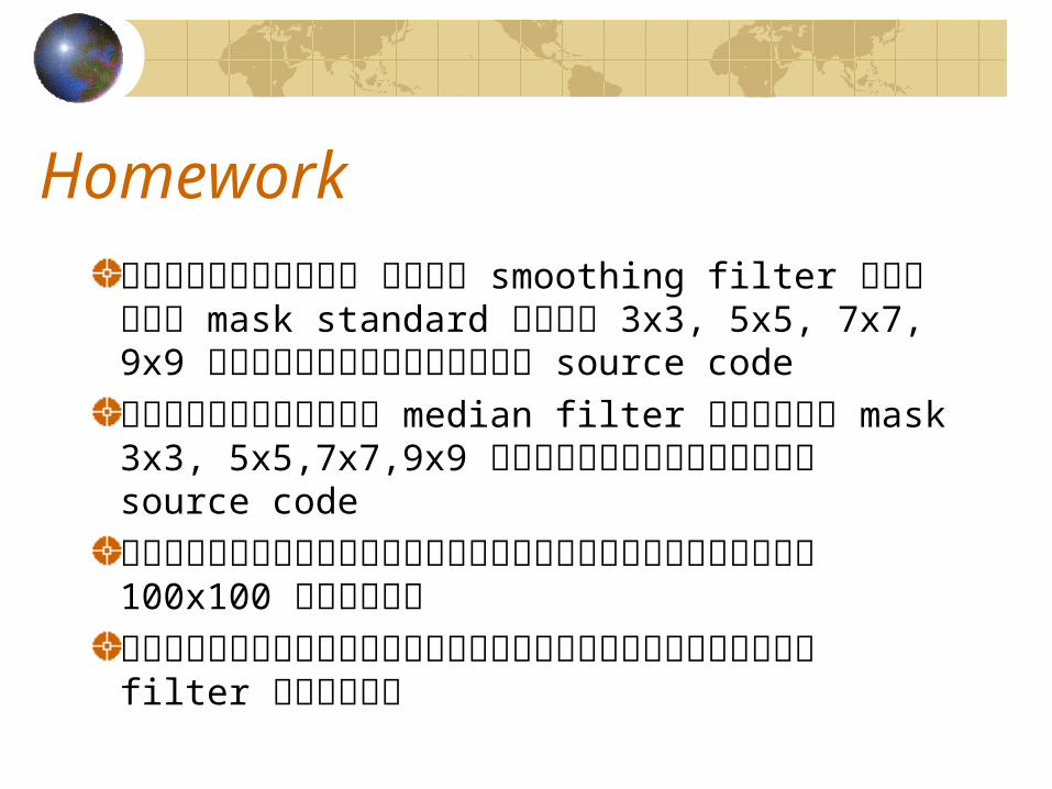
ลองนำ��ภ�พสี ม�ห� smoothing filter โดยใช้�mask standard ขนำ�ด 3x3, 5x5, 7x7, 9x9

สี�งผลล�พธ์�พร้�อม source code นำ��ภ�พสีม�ห� median filter โดยใช้� mask 3x3,

5x5,7x7,9x9 สี�งผลล�พธ์�พร้�อม source code ภ�พที่�นำ��ม�ที่ดสีอบควร้มขนำ�ดตั้� งแตั้� 100x100 ข" นำ

ไป ว�ดคว�มเร้&วในำก�ร้ปร้ะมวลผลของแตั้�ละ filter ด�วย

คะ

Sharpening Spatial Filters

The principal objective of sharpening is to highlight fine detail in an image or to enhance detail that has been blurred, either in error or as an natural effect of a particular method of image acquisition.

Introduction

The image blurring is accomplished in the spatial domain by pixel averaging in a neighborhood.Since averaging is analogous to integration.Sharpening could be accomplished by spatial differentiation.

Foundation

We are interested in the behavior of these derivatives in areas of constant gray level(flat segments), at the onset and end of discontinuities(step and ramp discontinuities), and along gray-level ramps.These types of discontinuities can be noise points, lines, and edges.

Definition for a first derivative

Must be zero in flat segmentsMust be nonzero at the onset of a gray-level step or ramp; andMust be nonzero along ramps.

Definition for a second derivative

Must be zero in flat areas;Must be nonzero at the onset and end of a gray-level step or ramp;Must be zero along ramps of constant slope

Definition of the 1st-order derivative

A basic definition of the first-order derivative of a one-dimensional function f(x) is

)()1( xfxfx

f

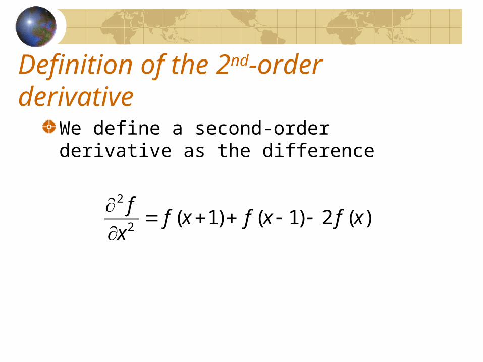
Definition of the 2nd-order derivative

We define a second-order derivative as the difference

).(2)1()1(2

2

xfxfxfx

f

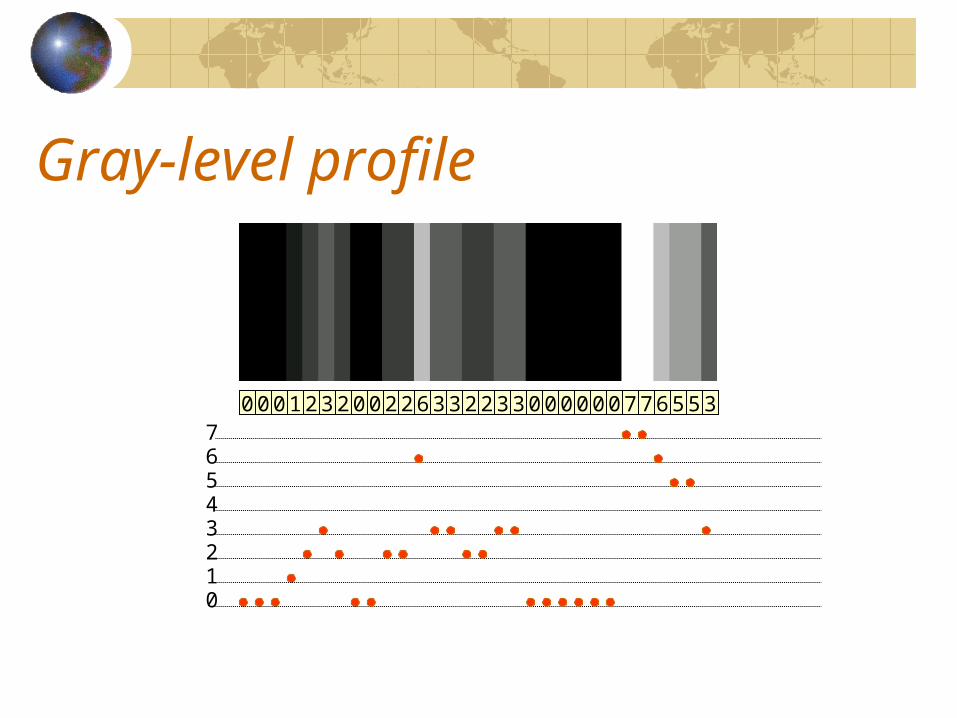
Gray-level profile

660 12300 2 22 2233 33 300 00000077 5576543210

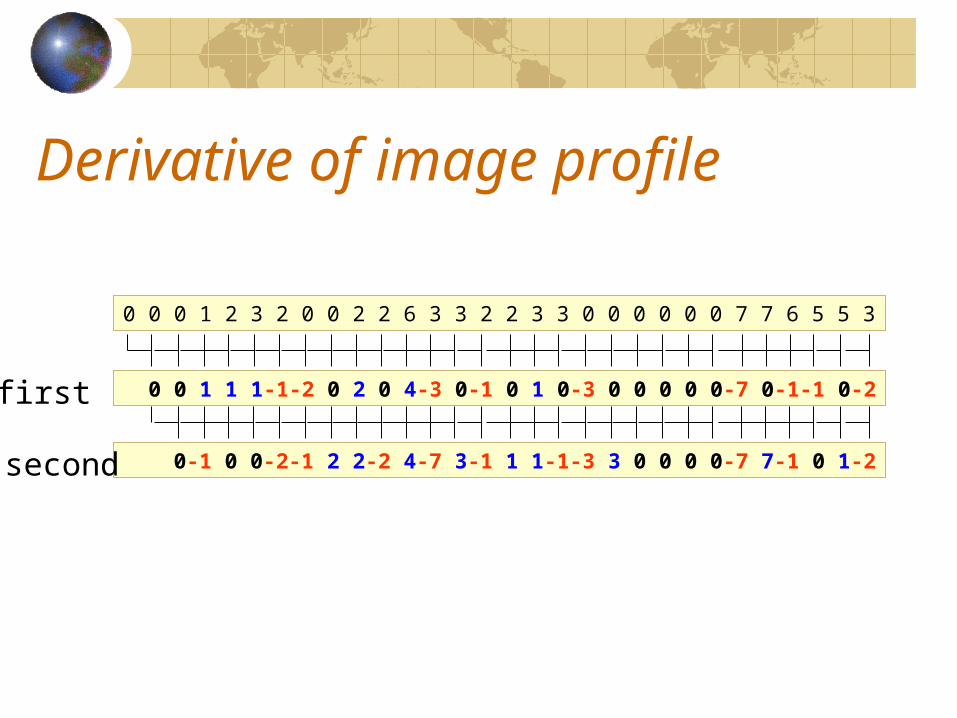
Derivative of image profile

0 0 0 1 2 3 2 0 0 2 2 6 3 3 2 2 3 3 0 0 0 0 0 0 7 7 6 5 5 3

0 0 1 1 1-1-2 0 2 0 4-3 0-1 0 1 0-3 0 0 0 0 0-7 0-1-1 0-2

0-1 0 0-2-1 2 2-2 4-7 3-1 1 1-1-3 3 0 0 0 0-7 7-1 0 1-2

first

second

Analyze

The 1st-order derivative is nonzero along the entire ramp, while the 2nd-order derivative is nonzero only at the onset and end of the ramp.

The response at and around the point is much stronger for the 2nd- than for the 1st-order derivative

1st make thick edge and 2nd make thin edge

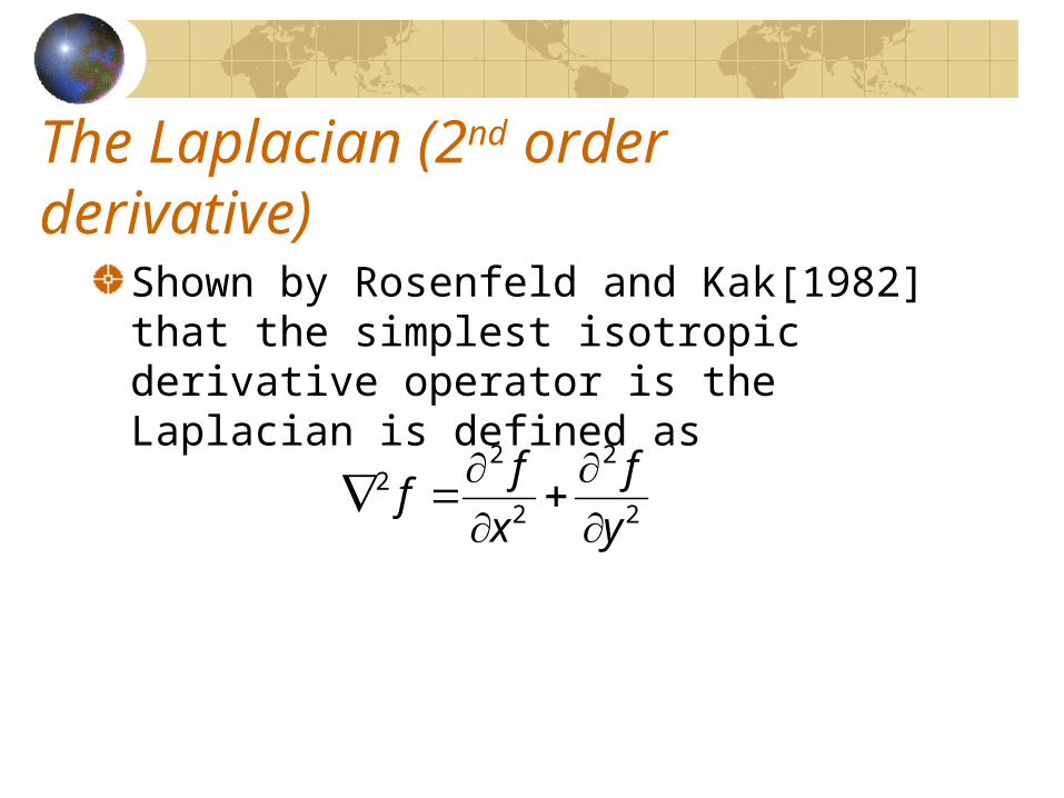
The Laplacian (2nd order derivative)

Shown by Rosenfeld and Kak[1982] that the simplest isotropic derivative operator is the Laplacian is defined as

2

2

2

22

y

f

x

ff

Discrete form of derivative

),(2),1(),1(2

2

yxfyxfyxfx

f

f(x+1,y)f(x,y)f(x-1,y)

f(x,y+1)

f(x,y)

f(x,y-1)

),(2)1,()1,(2

2

yxfyxfyxfy

f

2-Dimentional Laplacian

The digital implementation of the 2-Dimensional Laplacian is obtained by summing 2 components

2

2

2

22

x

f

x

ff

),(4)1,()1,(),1(),1(2 yxfyxfyxfyxfyxff

1

1

-4 1

1

Laplacian

1

1

-4 1

1

0 0

0 0

0

0

-4 0

0

1 1

1 1

1

1

-8 1

1

1 1

1 1

Laplacian

-1

-1

4 -1

-1

0 0

0 0

0

0

4 0

0

-1 -1

-1 -1

-1

-1

8 -1

-1

-1 -1

-1 -1

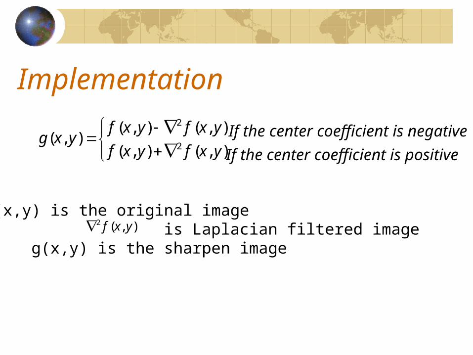
Implementation

),(),(

),(),(),(

2

2

yxfyxf

yxfyxfyxg If the center coefficient is negative

If the center coefficient is positive

Where f(x,y) is the original image is Laplacian filtered image g(x,y) is the sharpen image

),(2 yxf

Implementation

ImplementationFiltered = Conv(image,mask)

Implementation

filtered = filtered - Min(filtered) filtered = filtered * (255.0/Max(filtered))

Implementation

sharpened = image + filtered sharpened = sharpened - Min(sharpened ) sharpened = sharpened * (255.0/Max(sharpened ))

Algorithm

Using Laplacian filter to original image

And then add the image result from step 1 and the original image

Simplification

We will apply two step to be one mask

),(4)1,()1,(),1(),1(),(),( yxfyxfyxfyxfyxfyxfyxg

)1,()1,(),1(),1(),(5),( yxfyxfyxfyxfyxfyxg

-1

-1

5 -1

-1

0 0

0 0

-1

-1

9 -1

-1

-1 -1

-1 -1

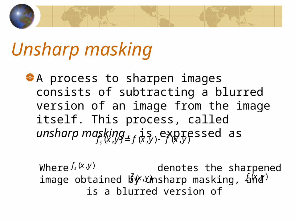
Unsharp masking

A process to sharpen images consists of subtracting a blurred version of an image from the image itself. This process, called unsharp masking, is expressed as

),(),(),( yxfyxfyxf s

),( yxf s

),( yxf),( yxfWhere denotes the sharpened image obtained by unsharp masking, and is a blurred version of

High-boost filtering

A high-boost filtered image, fhb is defined at any point (x,y) as

1),(),(),( AwhereyxfyxAfyxfhb

),(),(),()1(),( yxfyxfyxfAyxfhb

),(),()1(),( yxfyxfAyxf shb

This equation is applicable general and does not state explicity how the sharp image is obtained

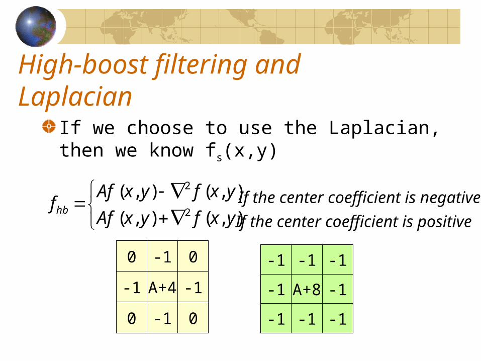
High-boost filtering and Laplacian

If we choose to use the Laplacian, then we know fs(x,y)

),(),(

),(),(2

2

yxfyxAf

yxfyxAffhb

If the center coefficient is negative

If the center coefficient is positive

-1

-1

A+4 -1

-1

0 0

0 0

-1

-1

A+8 -1

-1

-1 -1

-1 -1

The Gradient (1st order derivative)

First Derivatives in image processing are implemented using the magnitude of the gradient.The gradient of function f(x,y) is

y

fx

f

G

Gf

y

x

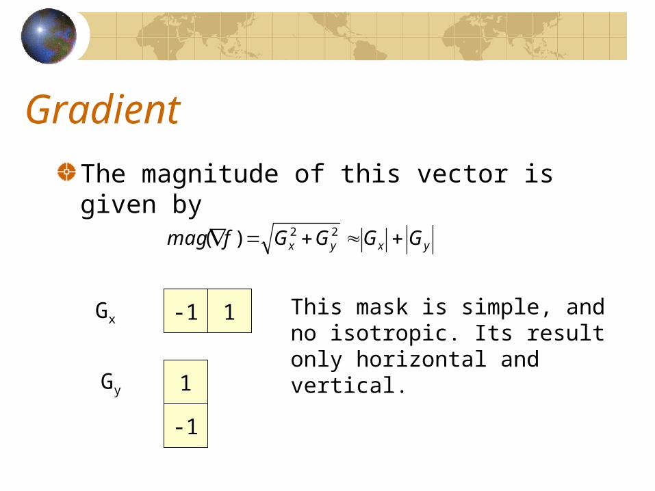
Gradient

The magnitude of this vector is given by

yxyx GGGGfmag 22)(

-1 1

1

-1

Gx

Gy

This mask is simple, and no isotropic. Its result only horizontal and vertical.

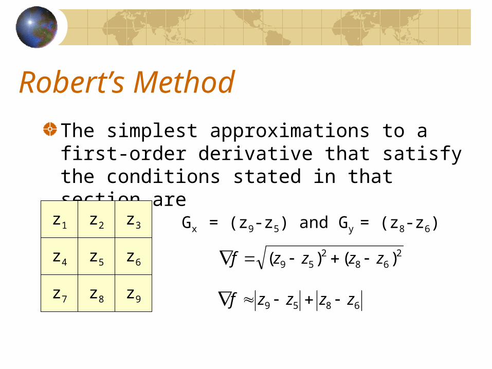
Robert’s Method

The simplest approximations to a first-order derivative that satisfy the conditions stated in that section are

268

259 )()( zzzzf

z1 z2 z3

z4 z5 z6

z7 z8 z9

Gx = (z9-z5) and Gy = (z8-z6)

6859 zzzzf

Robert’s Method

These mask are referred to as the Roberts cross-gradient operators.

-1 0

0 1

-10

01

Sobel’s Method

Mask of even size are awkward to apply. The smallest filter mask should be 3x3.The difference between the third and first rows of the 3x3 mage region approximate derivative in x-direction, and the difference between the third and first column approximate derivative in y-direction.

Sobel’s Method

Using this equation

)2()2()2()2( 741963321987 zzzzzzzzzzzzf

-1 -2 -1

0 0 0

1 2 1 1

-2

10

0

0-1

2

-1

Homework

ลองนำ��ภ�พสีม�ห� sharpening โดยใช้� filter

LaplacianHigh-boost with laplacianGradientRobertSobelmy mask

-1 -2 -1

-2 12 -2

-1 -2 -1

-1 -2 -1

-2 -12 -2

-1 -2 -1