spatial aspects of the productivity slowdown: an … · casetti 1984a, 1984b) indicated that higher...

Taylor & Francis, Ltd. and Association of American Geographers are collaborating with JSTOR to digitize, preserve and extend access to Annals of the Association of American Geographers.

http://www.jstor.org

Spatial Aspects of the Productivity Slowdown: An Analysis of U.S. Manufacturing Data Author(s): Emilio Casetti and John Paul Jones III Source: Annals of the Association of American Geographers, Vol. 77, No. 1 (Mar., 1987), pp.

76-88Published by: on behalf of the Taylor & Francis, Ltd. Association of American GeographersStable URL: http://www.jstor.org/stable/2569203Accessed: 26-03-2015 15:14 UTC

Your use of the JSTOR archive indicates your acceptance of the Terms & Conditions of Use, available at http://www.jstor.org/page/info/about/policies/terms.jsp

JSTOR is a not-for-profit service that helps scholars, researchers, and students discover, use, and build upon a wide range of contentin a trusted digital archive. We use information technology and tools to increase productivity and facilitate new forms of scholarship.For more information about JSTOR, please contact [email protected].

This content downloaded from 157.253.50.51 on Thu, 26 Mar 2015 15:14:57 UTCAll use subject to JSTOR Terms and Conditions

http://www.jstor.org

http://www.jstor.org/action/showPublisher?publisherCode=taylorfrancis

http://www.jstor.org/action/showPublisher?publisherCode=aag

http://www.jstor.org/stable/2569203

http://www.jstor.org/page/info/about/policies/terms.jsp


Spatial Aspects of the Productivity Slowdown: An Analysis of U.S. Manufacturing Data Emilio Casetti* and John Paul Jones lilt

*Department of Geography, Ohio State University, Columbus, OH 43210-1360 tDepartment of Geography, University of Kentucky, Lexington, KY 40506

Abstract. We investigate the spatial differentiation in the rates of change of manufacturing productivity growth in the U.S. Using an application of the "expansion method," we focus on the relation between the productivity slowdown and the Snowbelt-Sunbelt shift that materialized at approximately the same time during the mid-1960s. We find that the spatial patterns of manufacturing productivity acceleration were different before and after the mid-1960s, and we suggest that a redirection of capital flows is the mechanism behind the spatial patterns observed and the interrelations between the slowdown and the shift.

Key Words: productivity slowdown, Snowbelt-Sunbelt shifts, capital flows, expansion method, trend surface expansions.

THE recent slowdown in productivity growth and the decline of the Northeast and Midwest

are major economic issues confronting the United States. They are causes, effects, and symptoms of the erosion in the position of strength and world dominance that the U.S. economy enjoyed in the period immediately following World War II. Both contributed significantly to the inflationary pressures and high unemployment levels of recent years. The continued prosperity of the U.S. economy de- pends largely upon the extent to which the productivity slowdown and the decline of the old industrial core regions are counteracted and re- versed.

The crisis in the Northeast and Midwest has been associated with accelerated economic and population growth in some regions in the South and West. The combination of these trends, often referred to as the Snowbelt-Sunbelt shift, began at approximately the same time as the productivity slowdown in the mid- 1960s. The temporal coincidence between the Snowbelt-Sunbelt shift and the productivity slowdown is illustrated in Figure 1. In it, the percentage net migration rates for two Snowbelt census divisions (the Middle Atlantic and East North-Central) and for two Sunbelt divisions (the East and West South-Central) are plotted at

the midpoint of the ten-year census periods from 1940. Note that whereas the Snowbelt divisions have declining rates of net migration, the Sunbelt regions display a strong turnaround from negative to positive rates. Also shown in Figure 1 are estimates of the U.S. annual rates of growth in labor productivity in both durable and nondurable manufacturing. These estimates, covering the 1950- 66, 1966-73, and 1973-77 time periods, come from Kendrick (1980, 14). Both manufacturing sectors show a decline in growth rates, and the decline is roughly contemporaneous with the shifts in regional net migration rates.

This temporal coincidence points to a possible relation between the two and suggests that the productivity slowdown may also possess significant spatial dimensions. Although considerable attention has been devoted to understanding Snowbelt- Sunbelt shifts, little work has been done on the spatial dimensions of the productivity slowdown and on the relationships between the slowdown and the shifts. These relatively neglected issues are the focus of this paper.

The productivity slowdown is a decline in the rate of growth of productivity that constitutes a negative productivity acceleration. In this paper we aim to identify significant spatial patterns of

Annals of the Association of American Geographers, 77(1), 1987, pp. 76-88 (D Copyright 1987 by Association of American Geographers

76



Productivity Slowdown 77

15.0 -

3.5 10.0 NON-DURABLE

5.0-

MA _ _ _ _ _r 3 ~~~~~DURABLE //

DECENNIAL PERCENT ENC NET MIGRATION: 2 25 AVERAGE ANNUAL

0.0 PERCENT SELECTED CENSUS DIVISIONS PRODUCTIVITY GROWTH:

DURABLE AND NON-DURABLE

2.0 MANUFACTURING -5.0 1

ESC --- _ __ / I -10.0

-15.0

1940 1950 1960 1970 1980

Figure 1. The productivity slowdown and Snowbelt-Sunbelt shifts. Migration data are percentage rates of net migration by census period for the Middle Atlantic (MA), East North Central (ENC), West South Central (WSC), and South Atlantic (SA) census divisions. Productivity data are average annual percentage growth rates by manufacturing type and are taken from Kendrick (1980).

productivity acceleration for two time periods, one preceding and the other following both the Snow- belt-Sunbelt shift and the productivity slowdown. We use trend surface expansions to estimate the spatial variation of a differential equation from which measures of acceleration are extracted. As only statistically significant spatial variation is employed to derive the acceleration measures, the resulting spatial patterns can be presumed to re- veal substantive realities rather than averaged noise. Our results show that before the onset of the Snowbelt-Sunbelt shift the rate of productivity growth was highest in the old industrial core regions, whereas after the shift it became highest in portions of the Sunbelt. In the concluding portion of the paper, we articulate two hypotheses con- cerning the linkage between the shift and the spatial aspects of productivity dynamics.

The Productivity Slowdown

Productivity growth is a trait of modem economies. This is not to say that episodes of declining productivity cannot be found in the modern world. In contemporary developed countries, however, productivity growth constitutes the rule rather than the exception. Increasing productivity growth generally identifies healthy economic sectors, regions, or countries.

The productivity slowdown in the U.S. econ-

omy began in the mid-1960s. It soon caused grave concern because it was taken to signal a worsening of the competitive position of the U.S. economy vis a vis other countries and to reduce the possi- bility of noninflationary increases in wages and incomes. The productivity slowdown was interpreted as both cause and symptom of perverse economic trends that needed to be addressed, understood, and corrected.

The literature on the productivity slowdown has been growing rapidly (see, e.g., Denison 1979; Federal Reserve Bank of Boston 1980; Kendrick and Grossman 1980; Maital and Meltz 1980; Moomaw 1980). Explanations have focused on the quality of labor inputs, the amount and direction of investments, and the impact of government regulation (Christainsen and Haveman 1981; Filer 1980; Baily 198 la). The main points of these explanations can be summarized as follows:

(1) A higher proportion of labor inputs has been contributed by women and younger people since the onset of the productivity slowdown. Increased labor participation by women resulted from struc- tural changes in American society; the larger proportion of younger people in the labor force has been due to the aging of the "baby boom" cohort. Some authors suggest that female and young workers contribute less productive labor inputs (Perry 1971; Perloff and Wachter 1980).

(2) The rate of capital formation has declined



78 Casetti and Jones

(Kopcke 1980; Baily 1981b; Boucher 1981; Frau- meni and Jorgenson 1981). Fresh capital has been diverted from directly productive investments into expenditures related to government regulations (Crandall 1980, 1981; Myers and Nakamura 1980; Christainsen and Haveman 1981; Link 1982c). Research and development expenditures have also declined (Mansfield 1965; Terleckyj 1974, 1982; NSF 1977; Griliches 1980a, 1980b; Clark and Griliches 1981; Link 1982a, 1982b).

(3) The pressures from unions, consumerists, environmentalists, and assorted social welfare proponents produced "excessive" government regulation and a business climate unfavorable to productivity growth (Freeman and Medoff 1979; Abramowitz 1981; Gollop and Roberts 1982).

The spatial dimensions of the productivity slowdown have attracted little attention. In an analysis at the Census Division level, Hulten and Schwab (1984) concluded that the slowdown in manufacturing labor productivity was almost ubiquitous, with only minor regional variations. On the other hand, the recent investigations of the spatial validity of the Verdoorn law described below suggest spatial patterning in the productivity slowdown and point toward possible linkages between this patterning and Snowbelt-Sunbelt shifts.

According to the Verdoorn law, productivity grows faster in economic sectors that are in the process of expanding. Cross-sectional state-level analyses (Casetti 1982b; Casetti and Jones 1983; Casetti 1984a, 1984b) indicated that higher productivity growth tends to be associated with higher output growth and that the productivity response to output growth tended to be higher in some Snowbelt regions before the mid-1960s and higher in some Sunbelt areas in subsequent years. This suggests that different spatial patterns of productivity dynamics prevailed before and after the onset of the productivity slowdown and of the Snowbelt-Sunbelt shift. As a productivity slowdown denotes a weakening of the competitive position of an economy, it is reasonable to expect changes in the spatial dynamics of productivity whenever the competitive position of different regions is significantly altered. The economic decline of the old industrial cores in the U.S. and the rapid expansion of some regions in the South strongly suggest sympathetic changes in productivity dynamics.

A relation between spatial patterns in productivity dynamics and national trends is also plau- sible. Prior to the mid-1960s, the productivity

acceleration in the industrial core regions, where most of the manufacturing is concentrated, was translated into a favorable productivity perform- ance at the national scale. Subsequently, productivity gains associated with a smaller but growing Sunbelt economy may not have been enough to compensate for the productivity slowdown in other parts of the country. If this is the case, then spatial differentials in productivity acceleration associated with the Snowbelt-Sunbelt shifts may have contributed to the national decline in productivity growth.

The Snowbelt-Sunbelt Shift

The shift of population and jobs from Snowbelt to Sunbelt constitutes a complex cluster of not- too-sharply defined spatial changes that are partly an acceleration and partly a reversal of previous trends (Sternlieb and Hughes 1975; Vining and Strauss 1977). The shift began in the mid-1960s, when population and economic activity started to move out of established industrial regions and large metropolitan agglomerations. At the same time other places - notably in the West, in the South, some mid-sized urban centers, and some nonmetropolitan areas - began to grow (Beale 1977; Berry and Dahman 1977; Chinitz 1978; Rees 1979; Sternlieb and Hughes 1975, 1978). The dispersal of population and economic activities out of old industrial cores is typical of the deglomerative trends that have been investigated and documented for a number of countries (Richardson 1980; Vining and Pallone 1982).

In many respects the Snowbelt-Sunbelt shift constitutes an unexpected reversal of long-run trends that shaped the spatial structure of the American socioeconomic system (Vining and Strauss 1977). Such a shift cannot be explained in terms of cu- mulative causation and growth pole theories, as these theories imply that the more developed areas will grow comparatively more and will induce growth in the territories around them. The failure of conventional regional development concepts to anticipate trends as significant as those underway in the U.S. has led to a variety of attempts to reformulate theories of regional growth (Richard- son 1980; Casetti 1981; Peet 1984).

The major determinants of regional growth and decline according to these new reformulations can be summarized as follows. The old industrial cores depend upon manufacturing activities that are especially vulnerable to competition from other




countries because of higher labor costs and more obsolete capital in such older manufacturing areas. Also, old industrial cores often experience stronger social and political pressures by groups committed to protecting the environment, the workers, and the less fortunate members of society. Despite the positive role such pressures play, they bring about higher business costs that compound the perverse dynamics experienced by these regions (Bluestone and Harrison 1982; Casetti 1984c; Peet 1983, 1984). New businesses and plants, however, that are dis- proportionately those economic activities in which the U.S. is strongly competitive tend to locate in a few Sunbelt areas that are experiencing spectac- ular growth.

It is generally believed that capital flows played a very important role in the Snowbelt-Sunbelt shift (Clark and Gertler 1983; Clark, Gertler, and Whiteman 1986, 210ff.). Capital leaving regions with poor business climates in the old industrial cores for more favorable environments in the Sun- belt produces job shifts that alter the traditional interregional migration streams. An influx of capital will, however, tend to increase the rate of productivity growth (Casetti and Jones 1983). Therefore, it seems reasonable to hypothesize that the faster-growing Sunbelt regions have recently experienced higher productivity acceleration than previously, whereas the opposite holds for the Snowbelt areas that are stagnating or declining.

The Model

Evaluating the spatial variation of productivity acceleration (the rate of change of the rate of growth) is not an easy task. The straightforward approach to measuring acceleration involves first obtaining growth rates for two consecutive time periods and then estimating the rate of change between the two. Because the calculation of a growth rate amplifies any noise present in the data, however, this approach amplifies noise in the original productivity data three times: (1) in producing the growth rates, (2) in obtaining acceleration measures, and (3) in computing rates of change of acceleration over space.

We assess spatial variation in the rates of change of productivity growth from cross-sections of levels of and rates of change in productivity. The noise amplification with this methodology is not greater than that involved in growth-rates analyses.

Let Y and L denote, respectively, value added

and labor inputs, so that labor productivity is given by

P = YIL. (1)

Let Z signify the logarithmic transformation of P:

Z = lnP. (2)

Denote the first and second derivative of a variable with respect to time t, as follows:

Z' = dZ/dt, and (3)

Z" = dZ'/dt. (4)

Since Z = lnP, the logarithmic derivative of productivity with respect to time, Z', is the percentage rate of change of productivity over time:

Z' = (l/P)(dPldt). (5)

The time derivative of Z' is the instantaneous rate of change of percentage productivity change and consequently is an indicator of productivity acceleration. Z" is the productivity acceleration measure that we use in this paper.

The method employed to investigate the spatial variation of productivity acceleration involves (1) specifying an equation capable of yielding productivity acceleration by implicit derivation with respect to time and then (2) expanding the parameters of this equation to produce spatially differ- entiated estimates of productivity acceleration. The specifics of the method follow. Let

Z' = f(Z) (6)

be a differential equation relating percentage rate of change of productivity to the logarithm of productivity. Taking the derivatives with respect to time of both sides of Equation (6) we obtain

Z = g(Z,Z'), (7)

which expresses the measure of acceleration used in this investigation, Z", as some function of percentage rate of change of productivity, Z', and of the logarithm of productivity, Z. If Equation (6) defines Z' as an intrinsically -linear function of Z, acceleration estimates can be arrived at by ordinary multiple regression. To show it, let us specify f(Z) as a polynomial in Z

Z= ao+aZ+a2Z2+a3Z3+ ... (8)



80 Casetti and Jones,

so that

Z' = Z'(a I + 2a2Z + 3a3Z2 .). (9)

If cross-sectional values of Z' and Z are available, regression estimates of the a's in Equation (8) can be obtained and then employed using Equation (9) to obtain cross-sectional estimates of Z'. Specifically, acceleration estimates by area can be obtained from the estimated a's and from the Z and Z' values for the observations. However, Z" estimates obtained using this approach would be based on the assumption that the Z'(Z) relation specified by Equation (6) is stable over the spatial context considered. In other words, it assumes not only that the same functional specification of Z'(Z) is valid throughout the area under consideration but also that its parameters are spatially invariant.

The assumption that the same specification of Z'(Z) is valid throughout the period is not unrea- sonable, especially if the time interval considered is not too large. The specification of a functional relation in terms of a low-order polynomial is one of the simplest possible, and it is legitimate to use a simple function in the absence of reasons favor- ing a more complex function. No such reasons are apparent here. The assumption that Equation (8) should hold with the same parameters over the study area is, however, unduly restrictive.

Regional differences in economic structure and level of economic maturity, and differences stem- ming from historical and physical factors, suggest that the parameters of Equation (8) might not be spatially invariant. A reformulation of the model that allows the testing for, and estimation of, spatial parameter variation can be easily arrived at using the expansion method (Casetti 1972, 1982a). The approach used in this paper is a modification of the trend surface expansions discussed in Jones (1984).

The expansion method is a technique for generating more complex terminal models from sim- pler initial ones and involves redefining at least some of the parameters of the initial model as functions of relevant variables. The expanded parameters are then put back into the initial model to produce a terminal model. For appropriate initial models and functional specifications of the expansions, the terminal model is intrinsically linear and consequently its parameters can be estimated by ordinary multiple regression. In the trend surface expansions the parameters of the initial

model are expanded into polynomials in the coordinates of areal centroids.

Suppose, for instance, that we select the differential equation

Z= ao+aZ+a2Z2 (1 0)

as the initial model. Equation (10) is a special case of (8) and is the equation that will be used in the empirical analyses described later. A quadratic trend surface expansion of (10) involves redefining the parameters ao, a,, and a2 of (10) into quadratic polynomials in the spatial x-y coordinates of the observations, which in this study are state centroids:

ao = a00 + a0jX + a02Y + a03X2

+ a04Y2 + a05XY, (11)

al = a10 + aj1X + a12Y + aj3X2

+ a14Y2 + a15XY, and (12)

a2 = a20 + a2IX + a22Y + a23X2

+ a24Y2 + a25XY. (13)

Replacing the right-hand sides of Equations (11), (12), and (13) for the corresponding parameters in Equation (10) yields an 18-term terminal model. This model is capable of estimation by ordinary multiple regression. Specifically, stepwise regression or backward selection can be used to estimate the terminal model that has the largest R2 and all regression coefficients significantly different from zero. The appropriate parameters in this estimated equation can then be substituted into the expansion Equations (11), (12), and (13) in order to specify the spatial variation of the parameters of the initial model.

The literature on polynomial regressions and on trend surface analyses notes that successive pow- ers of temporal and/or spatial coordinates can produce highly correlated variables. This multicollinearity can pose a serious problem if all the terms in a polynomial are included in, a regression. The techniques suggested for obviating this problem have included orthogonal polynomials, ridge regressions, and principal components analysis.

The approach adopted here involves obtaining varimax rotated principal components of the pow- ers of the observations' coordinates and then using these to expand the initial model. Expansions in terms of rotated principal components were carried out by redefining the coefficients ao, a,, and




a2 of Equation (10) as linear functions of variables PI, P2, -.- :

ao = a00 + ao pI + a02P2 + *-- , (14)

a, = al0 + allp, + aI2p2 + ...,and (15)

a2 = a20 + a2IpI + a22p2 + *- , (16)

where the p's are rotated principal components of X, Y, X2, Y2, and XY when quadratic trend surface expansions are contemplated; of X, Y, X2, y2, XY, X3, Y3, X2Y, and XY2 when cubic trend surface expansions are desired, and so on.

Expansions in terms of rotated principal components of the coordinates' transformations are vastly preferable to using the rotated principal components of variables appearing in trend surface expansions. They constitute a convenient approach of general applicability to the investigation of the spatial or temporal variation of the parameters of an initial equation using the expansion method. Rotated principal components of the co- ordinate transformations corresponding to a trend surface of a given order for a given spatial setting needs to be done only once and can be used re- peatedly to carry out expansions of different initial models. Such reusability of the rotated components routinizes the application of the expansion method to investigating the spatial variation of a model's parameters. It is also likely to solve multicollinearity problems that do not arise from the initial model itself. This approach proved ade- quate to solve the multicollinearity problem in the empirical analyses here.

The stepwise regression and backward selection procedures employed in the estimation of terminal models rely upon t (or F) tests for determining the variables that are significantly associated with population parameters and should be retained. These significance tests are based, however, on the assumption that the error terms associated with the observations are independent; a significant spatial autocorrelation of regression residuals is inconsis- tent with such independence. Spatial autocorrelation of the regression residuals could result from error terms produced by spatially autoregressive processes or by misspecification of the regression model. A failure to incorporate systematic parameter variation in a regression model constitutes potential misspecification.

This reasoning suggested that tests for autocorrelation should be performed for all the regressions reported in this investigation. The tests carried out were based on the I statistic (Cliff and Ord

1981, 201ff.). For each regression four tests were executed, each based on a different specification of the weight matrix, W:

W(ij) = 1 if d(ij)<200 miles,

else W(ij)=0,

W(ij) = 1 if d(ij)<400 miles,

else W(ij)=0, W(ij) = 1 if d(ij)<600 miles,

else W(ij)=0, and W(ij) = 1 if d(ij) < 800 miles,

else W(ij) = 0

where W(ij) is the entry of the weight matrix corresponding to observations i and j, and d(inj) is the distance in miles between the locations of observations i and j. Here the observations are states, and the distances are between-state centroids. These specifications of the weight matrix W allow testing for spatial autocorrelation at the local scale (200 and 400 mi.) and at the regional scale (600 and 800 mi.), and have already proved useful for detecting spatial autocorrelation among residuals in regressions employing state level data (Jones 1983).

Analysis

The purpose of the empirical analysis presented in this section is (1) to determine whether statistically significant spatial patterns of productivity acceleration exist and (2) whether they differ before and after the onset of the Snowbelt-Sunbelt shift and of the productivity slowdown. It is useful to point out that the analyses here, as well as those by Hulten and Schwab (1984), are based on aggregate manufacturing data and do not address the comparative impacts of spatial variation in industry mixes. Undoubtedly, if these investigations are pursued further, attention has to be given to industry mix effects and to the spatial impacts of industry differentials in productivity dynamics. The occurrence of significant spatial patterns of productivity acceleration needs, however, to be investigated and established first.

The primary data used in our analyses are (1) the number of manufacturing production workers and the aggregate manufacturing value added for the years 1954, 1963, 1967, and 1977 for the 48 coterminous states of the U.S. plus the District of




Columbia and (2) the geographical coordinates of these areal units.

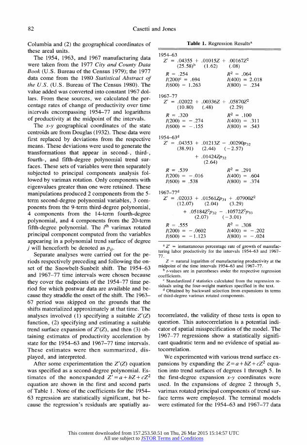
The 1954, 1963, and 1967 manufacturing data were taken from the 1977 City and County Data Book (U.S. Bureau of the Census 1979); the 1977 data come from the 1980 Statistical Abstract of the U.S. (U.S. Bureau of The Census 1980). The value added was converted into constant 1967 dol- lars. From these sources, we calculated the percentage rates of change of productivity over time intervals encompassing 1954-77 and logarithms of productivity at the midpoint of the intervals.

The x-y geographical coordinates of the state centroids are from Douglas (1932). These data were first replaced by deviations from the respective means. These deviations were used to generate the transformations that appear in second-, third-, fourth-, and fifth-degree polynomial trend surfaces. These sets of variables were then separately subjected to principal components analysis fol- lowed by varimax rotation. Only components with eigenvalues greater than one were retained. These manipulations produced 2 components from the 5- term second-degree polynomial variables, 3 components from the 9-term third-degree polynomial, 4 components from the 14-term fourth-degree polynomial, and 4 components from the 20-term fifth-degree polynomial. The ith varimax rotated principal component computed from the variables appearing in a polynomial trend surface of degree j will henceforth be denoted as Pij

Separate analyses were carried out for the periods respectively preceding and following the onset of the Snowbelt-Sunbelt shift. The 1954-63 and 1967-77 time intervals were chosen because they cover the endpoints of the 1954-77 time period for which postwar data are available and because they straddle the onset of the shift. The 1963- 67 period was skipped on the grounds that the shifts materialized approximately at that time. The analyses involved (1) specifying a suitable Z'(Z) function, (2) specifying and estimating a suitable trend surface expansion of Z'(Z), and then (3) obtaining estimates of productivity acceleration by state for the 1954-63 and 1967-77 time intervals. These estimates were then summarized, dis- played, and interpreted.

After some experimentation the Z'(Z) equation was specified as a second-degree polynomial. Es- timates of the nonexpanded Z' = a + bZ + CZ2 equation are shown in the first and second parts of Table 1. None of the coefficients for the 1954- 63 regression are statistically significant, but because the regression's residuals are spatially au-

Table 1. Regression Resultsa

1954-63 Z'= .04355 + .OlOlSZ + .00167Z2

(25.58)b (1.62) (.08)

R= .254 R2 = .064 I(200)C = .694 I(400) = 2.018 I(600) = 1.263 I(800) = .234

1967-77 Z'= .02022 + .00336Z + .05870Z2

(10.80) (.48) (2.29)

R= .320 R2 = .100 I(200) = - .274 I(400) = .311 I(600) = - .155 I(800) = .543

1 954-63 d

Z= .04353 + .01213Z- .0029-P32 (38.91) (2.44) (- 2.57)

+ .01424Zp32 (2.64)

R= .539 R2 = .291 I(200) = - .016 I(400) = .604 I(600) = .538 I(800) = .374

1967-77 d Z'= .02033 + .01561Zp31 + .07900Z2

(12.07) (2.04) (3.29)

+ .05184Z2p32 - . 10572Z2p33 (2.07) (-3.01)

R .555 R2 = .308 I(200) = - .0602 I(400) = - .202 1(600) = -1.123 I(800) = -.024

a Z' = instantaneous percentage rate of growth of manufacturing labor productivity for the intervals 1954-63 and 1967- 77.

Z = natural logarithm of manufacturing productivity at the midpoint of the time intervals 1954-63 and 1967-77.

b t-values are in parentheses under the respective regression coefficients.

C Standardized I statistics calculated from the regression residuals using the four-weight matrices specified in the text.

d Obtained by backward selection from expansions in terms of third-degree varimax rotated components.

tocorrelated, the validity of these tests is open to question. This autocorrelation is a potential indicator of spatial misspecification of the model. The 1967-77 regressions show a statistically significant quadratic term and no evidence of spatial autocorrelation.

We experimented with various trend surface expansions by expanding the Z = a + bZ + cZ2 equation into trend surfaces of degrees 1 through 5. In the first-degree expansion x-y coordinates were used. In the expansions of degree 2 through 5, varimax rotated principal components of trend surface terms were employed. The terminal models were estimated for the 1954-63 and 1967-77 data




using backward selection and retaining the regression step with the largest R2 in which all variables are significant at p S .05. Spatial autocorrelation tests on the residuals from these ten regressions yielded no significant autocorrelation for any of the four weight configurations considered.

The regressions for the early period indicate the existence of spatial variation in the parameters of the initial equation even for expansions in terms of a first-degree polynomial. For the latter period only the expansions of third degree or higher in- volve spatial terms. The statistically significant spatial terms demonstrate the existence of spatial instability in the initial model's parameters.

Individual accelerations by state were obtained from the derivatives with respect to time of the regression equations, using estimated regression coefficients and productivity data as shown in Equation (9). The acceleration estimates change somewhat with different expansions. The overall spatial patterns that they produce, however, are quite stable for expansions of sufficiently high degree. Specifically, the same states tend to have highest and lowest accelerations over the same time period across all the expansions into trend surfaces of third degree or higher. Therefore, we selected the third-degree trend surface expansions for further consideration. The regression results corresponding to these expansions are shown in the third and fourth parts of Table 1. Acceleration estimates based on these regressions were computed for states, ranked, and mapped by quartiles. The maps for the 1954-63 and 1967-77 periods are shown respectively in Figures 2 and 3.

Figure 2 reveals a strong north-south pattern,

with larger productivity accelerations found in New England, the upper Midwest, and the Northwest. Lower accelerations prevail in the South and West. Some elements of this pattern remain in the 1967- 77 map (Fig. 3), in which the states along the Canadian border retain high levels of acceleration relative to the remainder of the country and some southern states retain low values. In the 1967-77 period, however, high accelerations are also found in Texas and Louisiana, two states located in a region that previously had consistently low scores, whereas acceleration values in the lowest quartile materialize in some New England and western states.

A comparative picture of acceleration changes is provided in Figure 4. This map is based on an index constructed by first converting the 1954-63 and 1967-77 acceleration values to "standardized" accelerations and then taking the difference between the two standardized accelerations for each state. Standardized accelerations are in deviation from the U.S. mean divided by the standard deviation for the U.S.

This index is unaffected by the overall national decline in acceleration during the study period. Minor changes (from - 0. 10 to 0. 10) characterize those states that maintained their relative position between 1954 and 1977 (these states are shown in white in Fig. 4). Figure 4 reveals that states with standardized acceleration stability can be found in the West, South, and North-Central Census Re- gions, whereas moderate or large declines domi- nate in New England. Moderate increases characterize the midsection of the country (Illi- nois, Iowa, Kentucky, and Missouri), some west-

Table 2. Productivity Acceleration by Regions and Divisions

1954-63 1967-77 ACa SACb AC SAC

Northeast Region .4447 .62 -.0283 - .23 New England .5149 .72 -.0601 - .45 Middle Atlantic .3044 .42 .0353 .23

North-Central Region .2638 .36 .0467 .31 East North-Central .2106 .28 .0373 .24 West North-Central .3018 .42 .0534 .35

South Region -.4547 -.67 -.0070 - .07 South Atlantic -.3649 -.54 -.0258 -.21 East South-Central -.3811 -.56 -.0803 - .60 West South-Central -.7302 - 1.06 .1089 .75

West Region .1006 .13 -.0019 -.04 Mountain -.0981 -.16 .0145 .08 Pacific .6306 .88 - .0458 - .35

a Acceleration times 100. bStandardized acceleration (acceleration in deviation from the U.S. mean divided by the standard deviation for the U.S.).




-2.52 -0.22 0.14 0.42 2.14

Figure 2. Estimates of productivity acceleration for the 1954-1963 time period.

ern states (Arizona, Nevada, and Utah), and Oklahoma and North Dakota. Increases of more than 1.00 are confined to the Sunbelt states of Florida, Alabama, Louisiana, Texas, New Mex- ico, and to Wyoming. Declines, on the other hand, occur to a larger extent on the northeastern sea- board and in the southern states of Arkansas, Mis- sissippi, Virginia, and the Carolinas. The largest declines are confined to northern states: Oregon, Idaho, South Dakota, Maine, and New Hamp- shire. Thus, although standardized acceleration increases, decreases, and stability can be found in many areas of the country, the overall picture is one of increases in a handful of southern states combined with a contiguous region of decline or at best stability in the industrial and northern states of the East.

A picture of the change in productivity acceleration at the census region and census division level of resolution is given in Table 2. The acceleration measures for the 1954-63 and 1967-77 time periods (shown in Cols. 1 and 3 of Table 2) were obtained by taking the mean of the acceleration values for the states in each region and division; columns 2 and 4 of the table contain

standardized accelerations. Contrasting the entries in Columns 2 and 4 of Table 2 shows that the Northeast region suffered a major decline in productivity acceleration, that the South was the largest relative gainer in acceleration, and that the West and North-Central regions experienced little change. At the division level the clear "winner" is the West South-Central, while the clear "losers" are the New England and Pacific divisions. The overall picture emerging from Table 2 and from Fig- ures 2, 3, and 4 leads us to speculate about the mechanisms that produced it.

Discussion

Prosperous economies are characterized by productivity acceleration. This is why the productivity slowdown became the focus of public concern. Approximately coincident with the productivity growth slowdown were the shifts of population and jobs described earlier. How can we relate the productivity slowdown to these shifts?

The population and job shifts can be credited to the flow of capital out of areas formerly the focus




ACCELERATION x 1X _

-0.28 -0.07 0.01 0.03 0.44

Figure 3. Estimates of productivity acceleration for the 1967-1977 time period.

of agglomeration economies and later the focus of entrepreneurial concern over business costs and business climate. The worst business climates may have occurred, however, in Snowbelt areas with high productivity and productivity acceleration. This points toward a linkage between the population and employment shift and the productivity slowdown: Before the shift, the productivity gains were higher in the Snowbelt than in the Sunbelt. As the business climate slowly became more favorable in the Sunbelt, investments started to respond to business climate differentials more than to productivity differentials.

It seems legitimate to hypothesize that the capital movements away from areas of higher productivity growth toward areas where the productivity growth was slower or stagnating contributed significantly to the overall productivity dynamics in the U.S. Perhaps in the future the reverse will occur. As the Sunbelt matures and takes on a larger share of American manufacturing, the productivity acceleration in the Sunbelt may more than compensate for the lower productivity acceleration in some of the old industrial states. This could contribute to an increase in productivity growth at the national level.

Conclusion

Our findings indicate that the spatial patterns of manufacturing productivity acceleration in the U.S. were significantly different before vs. after the onset of the productivity slowdown and the Snow- belt-Sunbelt shift in population and jobs. A correspondence between productivity acceleration and regional growth was detected in the sense that some regions with lower growth in the earlier period, such as the West South-Central, were also characterized by low productivity acceleration. In the second period these areas shifted to both high growth and higher productivity acceleration. Con- versely, formerly high acceleration and high growth areas such as the Northeast shifted to "perverse" productivity dynamics and to lower rates of growth.

Perhaps the coincidence between Snowbelt- Sunbelt shifts and spatial patterns of productivity acceleration reflects the outflow of resources from areas of higher productivity acceleration and into areas with lower productivity acceleration but bet- ter business climates.

The debates over the causes of the productivity slowdown have pointed out that about 40 percent




CHANGE IN SCORES

-275 -1.00 -0.10 0.10 1.00 4.83

Figure 4. Difference in state standard scores of productivity acceleration between the 1954-1963 and 1967-1977 time periods. A negative value indicates a lower standard score for the latter period, and a positive value indicates a higher standard score for the latter period. States with little change in standard scores are blank.

of the decline in growth since 1965 cannot be explained by traditional aggregate-level methods. The failure of past research to treat productivity growth as a spatially complex phenomenon may have contributed to the inadequacy of these analyses. The redirection of capital flows that began during the 1960s is a spatial force with major systemic impacts. Rather than treating productivity as an as- patial phenomenon unrelated to the spatial shifts in population and jobs in this country, further research should relate productivity to the regional dimensions of economic and demographic dynamics.

References

Abramowitz, M. 1981. Welfare quandaries and productivity concerns. American Economic Review 71:1-17.

Baily, M.N. 1981a. Productivity and the services of capital and labor. Brookings Papers on Economic Activity 1:1-65.

. 198 lb. The productivity growth slowdown and

capital accumulation. American Economic Review 71:326-31.

Beale, C.L. 1977. The recent shifts of United States population to nonmetropolitan areas, 1970-75. In- ternational Regional Science Review 2:113-22.

Berry, B.J.L., and Dahman, D. 1977. Population re- distribution in the United States in the 1970's. Pop- ulation and Development Review 3:443-71.

Bluestone, B., and Harrison, B. 1982. The deindus- trialization of America: Plant closings, community abandonment, and the dismantling of basic industry. New York: Basic Books.

Boucher, T. 1981. Technical change, capital invest- ment, and productivity in the U.S. metalworking industries. In Aggregate and industry-level productivity analyses, ed. A. Dogramaci and N.R. Adam, pp. 93-122. Boston: Martinus Nijhoff.

Casetti, E. 1972. Generating models by the expansion method: Applications to geographical research. Geographical Analysis 4:81-91.

. 1981. A catastrophe model of regional dynamics. Annals of the Association of American Geog- raphers 71:572-79.

. 1982a. Mathematical modelling and the expansion method. In Statistics for geographers and social scientists, ed. R.B. Mandal. New Delhi: Concept Publishing.

. 1982b. Technological progress, capital deep- ening, and manufacturing growth in the U.S.: A




regional analysis. Environment and Planning A 14:1577-85.

. 1984a. Manufacturing productivity and snowbelt sunbelt shifts. Economic Geography 4:313-24.

. 1984b. Verdoorn law and the components of manufacturing productivity growth: A theoretical model and analysis of U.S. regional data. In Re- gional and industrial development theories, models and empirical evidence, ed. A.E. Andersson, W. Isard, and T. Puu. New York: Elsevier Science Publishers B.V. (North-Holland).

1984c. Peripheral growth in mature economies. Economic Geography 60:122-31.

Casetti, E., and Jones, J.P., III. 1983. Regional shifts in the manufacturing productivity response to output growth: Sunbelt versus snowbelt. Urban Ge- ography 4:285-301.

Chinitz, B. 1978. The declining Northeast: Demo- graphic and economic analyses. New York: Prae- ger.

Christainsen, G.B., and Haveman, R.H. 1981. Pub- lic regulations and the slowdown in productivity growth. American Economic Review 71:320-25.

Clark, G.L., and Gertler, M.S. 1983. Migration and capital. Annals of the Association of American Geographers 73:18-34.

Clark, G.L.; Gertler, M.S.; and Whiteman, J. 1986. Regional dynamics. Boston: Allen & Unwin.

Clark, K., and Griliches, Z. 1981. Productivity growth and R and D at the business level: Preliminary results from the PIMS data base. Paper presented at the National Bureau of Economic Research Con- ference on R and D, Patents and Productivity, Lenox, Mass.

Cliff, A.D., and Ord, J.K. 1981. Spatial processes. Models and applications. London: Pion.

Crandall, R.W. 1980. Regulation and productivity growth. In Federal Reserve Bank of Boston 1980, pp. 93-111.

. 1981. Pollution controls and productivity growth in basic industries. In Productivity measurement in regulated industries, ed. T.G. Cowing and R.E. Stevenson, pp. 347-68. New York: Academic Press.

Denison, E.F. 1979. Accounting for slower economic growth. The United States in the 1970's. Washing- ton, D.C.: The Brookings Institution.

Douglas, E.M. 1932. Boundaries, areas, geographic centers and altitudes of the United States and sev- eral states. United States Geological Survey, Bul- letin 817. Washington, D.C.: U.S. Government Printing Office.

Federal Reserve Bank of Boston. i980. The decline in productivity growth. Proceedings of a conference held in June at Edgartown, Mass. Conference Series no. 22. Boston: Federal Reserve Bank of Boston.

Filer, R.K. 1980. The downturn in productivity growth: A new look at its nature and causes. In Maital and Meltz 1980, pp. 109-23.

Fraumeni, B.M., and Jorgenson, D.W. 1981. Capital formation and U.S. productivity growth, 1948-1976. In Productivity analysis: A range of perspectives, ed. A. Dogramaci, pp. 49-70. Boston: Martinus Nijhoff.

Freeman, R.B., and Medoff, J.L. 1979. The two faces of unionisms. The Public Interest 57:69-93.

Gollop, F.M., and Roberts, M.J. 1982. Environmen- tal regulation and productivity growth: The case of fossil-fueled electric power generation. Boston College Working Paper no. 114, Chestnut Hill, Mass.

Griliches, Z. 1980a. R and D and the productivity slowdown. American Economic Review 70:343-48.

. 1980b. Returns to research and development expenditures in the private sector. In New developments in productivity measurement and analysis, ed. J.W. Kendrick and B.N. Vaccara, pp. 419-54. Chicago: University of Chicago Press.

Hulten, C.R., and Schwab, R.M. 1984. Regional productivity growth in U.S. manufacturing: 1951-78. The American Economic Review 74:152-62.

Jones, J.P. III. 1983. Parameter variation via the expansion method with tests for autocorrelation. Modeling and Simulation 14:853-57.

. 1984. A spatially varying parameter model of AFDC participation: Empirical analyses using the expansion method. The Professional Geographer 36:455-61.

Kendrick, J.W. 1980. Survey of the factors contrib- uting to the decline in U.S. Productivity Growth. In Federal Reserve Bank of Boston 1980, pp. 1- 21.

Kendrick, J.W., and Grossman, E.S. 1980. Produc- tivity in the United States. Trends and cycles. Bal- timore and London: The Johns Hopkins University Press.

Kopcke, R.W. 1980. Capital accumulation and potential growth. In Federal Reserve Bank of Boston 1980, pp. 26-53.

Link, A.N. 1982a. A disaggregated analysis of industrial R and D: Product versus process innovation. In The transfer and utilization of technical knowledge, ed. D. Sahal, pp. 45-62. Lexington, Mass.: D.C. Heath.

. 1982b. The impact of federal research and development spending on productivity. IEEE Trans- actions of Engineering Management EM-29:166- 69.

. 1982c. Productivity growth, environmental regulations, and the composition of R and D. Bell Journal of Economics 13:548-54.

Maital, S., and Meltz, N.M., eds. 1980. Lagging productivity growth. Causes and remedies. Cam- bridge, Mass.: Ballinger.

Mansfield, E. 1965. Rates of return from industrial research and development. American Economic Re- view 55:310-22.

Moomaw, R.L. 1980. The American productivity slowdown: Much ado about what? Working Paper no. 1447-3, The Urban Institute, Washington, D.C.

Myers, J.G., and Nakamura, L. 1980. Energy and pollution effects on productivity: A putty-clay approach. In New developments in productivity mea- surements and analysis, ed. J.W. Kendrick and B.N. Vaccara, pp. 463-98. Chicago: University of Chi- cago Press.

National Science Foundation. 1977. Relationships between R and D and economic growth/productivity. Washington, D.C.: U.S. Government Printing Of- fice.

Peet, R. 1983. Relations of production and the reloca-




tion of United States manufacturing industry since 1960. Economic Geography 59:113-43.

1984. Class struggle, the relocation of employment, and economic crisis. Science and Society 48:38-51.

Perloff, J.M., and Wachter, M.L. 1980. The productivity slowdown: A labor problem? In Federal Re- serve Bank of Boston 1980, pp. 115-42.

Perry, G.L. 1971. Labor force structure, potential output, and productivity. Brookings Papers on Eco- nomic Activity 3:533-65.

Rees, J. 1979. Regional industrial shifts in the U.S. and the internal generation of manufacturing in growth centers of the Southwest. In Interregional movements and regional growth, ed. W.C. Whea- ton. Washington, D.C.: The Urban Institute.

Richardson, H.W. 1980. Polarization reversal in de- veloping countries. Papers of the Regional Science Association 45:67-85.

Sternlieb, G., and Hughes, J.W. 1978. The new economic geography of America. In Revitalizing the northeast: Prelude to an agenda, ed. G. Sternlieb and J.W. Hughes, pp. 75-127. New Brunswick, N.J.: Center for Urban Policy Research, Rutgers University.

Sternlieb, G., and Hughes, J.W., eds. 1975. Post industrial America: Metropolitan decline and interregional job shifts. New Brunswick, N.J.: Center for Urban Policy Research, Rutgers University.

Terleckyj, N.E. 1974. Effects of R and D on the productivity growth of industries: An exploratory study. Washington, DC.: National Planning Association.

. 1982. R and D and the U.S. industrial productivity in the 1970's. In The transfer and utilization of technical knowledge, ed. D. Sahal, pp. 63-100. Lexington, Mass.: D.C. Heath.

U.S. Bureau of the Census. 1979. 1977 city and county data book. Washington, D.C.: U.S. Government Printing Office.

. 1980. Statistical abstract of the United States: 1980. Washington, D.C.: U.S. Government Print- ing Office.

Vining, D.R., and Pallone, R. 1982. Migration between core and peripheral regions: A description and tentative explanation of the patterns in 22 countries. Geoforum 13:339-410.

Vining, ID.R., and Strauss, A. 1977. A demonstration that the current decentralization of population in the United States is a clean break with the past. Environment and Planning A 9:751-58.



spatial aspects of the productivity slowdown: an … · casetti 1984a, 1984b) indicated that higher...

Documents