spatial and seasonal variations in copepod communities related to turbidity maximum along the...

Estuarine, Coastal and Shelf Science 68 (2006) 113e126www.elsevier.com/locate/ecss

Spatial and seasonal variations in copepod communities related toturbidity maximum along the Chikugo estuarine gradient in the

upper Ariake Bay, Japan

Md. Shahidul Islam a,*, Hiroshi Ueda b, Masaru Tanaka a

a Laboratory of Estuarine Ecology, Field Science Education and Research Center, Graduate School of Agriculture, Kyoto University,

Kyoto 606-8502, Japanb Center for Marine Environmental Studies, Ehime University, Bunkyo-cho 3, Ehime 790-8577, Japan

Received 26 October 2005; accepted 1 February 2006

Available online 5 April 2006

Abstract

We investigated the spatial and seasonal variations in copepod assemblage, distribution and diversity in a wide spatial gradient (including theturbidity maximum) in the Chikugo estuary. Copepod samples were collected over a period of 12 months from April 2004 to March 2005.Hydrographical parameters such as temperature, salinity, turbidity (nephelometric turbidity unit, NTU), chlorophyll-a (chl-a), and phaeopigment(PhP) were measured. Two contrasting spatial zones were identified along the estuary: a zone of turbidity maximum exists in the low salineupper estuary, which was characterized by significantly higher turbidity and PhP concentrations than the downstream euryhaline zone. Thesetwo contrasting zones are characterized by contrasting copepod assemblages. A low saline upstream (true-estuarine) assemblage was dominatedby an endemic calanoid coppeod, Sinocalanus sinensis, except during the summer when Psedodiaptomus inopinus dominated. In contrast,a euryhaline marine assemblage was observed in the downstream areas which was a multi-species assemblage dominated by common coastalmarine species (Acartia omorii, Oithona davisae, Paracalanus parvus, Pseudodiaptomus marinus, etc.). There were two distinct groups ofcopepods based on the seasonal abundance: those showing a clear seasonal variability and those not. Most of the dominant copepod taxa didnot show any well-defined seasonal pattern. Density, biomass, and diversity of copepods along the estuary are influenced by the hydrographicenvironments that are subject to significant spatio-temporal variations. Multivariate statistics showed that chl-a is the most significant predictorof overall copepod density, biomass and diversity as well as the density of dominant copepods and PhP is an additional predictor of copepodpopulation dynamics in the ETM zones. This study indicates that the hydrographic and biological characteristics of ETM differ from that in thedownstream marine areas and that spatial dynamics are more important than temporal dynamics in estuarine ecosystems.� 2006 Elsevier Ltd. All rights reserved.

Keywords: spatial and seasonal variation; copepod community; estuarine turbidity maximum; Chikugo estuary; Ariake Bay

1. Introduction

Copepods are among the most important secondary pro-ducers in coastal and marine ecosystems, representing an im-portant link between phytoplankton, microzooplankton andhigher trophic levels such as fish. The variability observed inthe distribution of copepod is due to a combination of both

* Corresponding author.

E-mail address: [email protected] (Md.S. Islam).

0272-7714/$ - see front matter � 2006 Elsevier Ltd. All rights reserved.

doi:10.1016/j.ecss.2006.02.002

hydrographical variables such as temperature, salinity, turbid-ity, etc. and biotic parameters such as food habits and foodavailability (Roff et al., 1988; Christou, 1998; Escribano andHidalgo, 2000; Beyst et al., 2001). However, copepod variabil-ity is difficult to relate to environmental factors because ofcomplex multifactorial influences (Kiorboe and Nielsen,1994). This is particularly true for estuarine environments be-cause they are extremely dynamic and heterogenous ecosys-tems, subject to strong fluctuations of biotic and abioticfactors; therefore, estuarine ecosystems are of particular inter-est for studying copepod population dynamics.

mailto:[email protected]

http://www.elsevier.com/locate/ecss

114 Md.S. Islam et al. / Estuarine, Coastal and Shelf Science 68 (2006) 113e126

Spatio-temporal variations and habitat types are among themost important factors that influence observed patterns of spe-cies abundance, composition and size structure of estuarineplanktons. Therefore, it is important that studies on estuarinecopepods include a wide spatial and temporal scale. It hasbeen shown that abundance and community structure of cope-pod display considerable variations on seasonal and spatialscales. Estuarine copepod communities are believed to be an-nually stable but show strong seasonal and spatial dynamics(Winkler et al., 2003) and, therefore, seasonal and spatial var-iations are generally more important than annual variations(David et al., 2005). Temperature, salinity, and food supplyare among the most important factors that influence the ob-served spatial and seasonal patterns in demographic variationsof copepods (Roddie et al., 1984; Hassel, 1986). Seasonal var-iations are mediated mainly by seasonal temperature variations(Durbin and Durbin, 1981) but salinity is also known to affectthe distribution of copepods in estuaries (Lawrence et al.,2004). Interspecific differences in salinity tolerance often ex-plain changes in the dominant species across the salinity gra-dient in estuary. Therefore, to achieve comprehensiveunderstanding on the dynamics of estuarine copepods, studiesshould be based on multivariate considerations (Manning andBucklin, 2005).

The estuarine turbidity maximum (ETM) is a ubiquitousfeature in dynamic estuarine ecosystems with substantial im-pacts on copepod abundance and distribution. Previous studieshave shown that planktonic predators encounter more prey un-der conditions of increased turbidity due to hydrodynamic ac-cumulation of particles (POM) (Rothschild and Osborn, 1988;Gasparini et al., 1999; Roman et al., 2001; Winkler et al.,2003). Hydrodynamic conditions also result in high abundanceand biomass of copepods in ETM (MacKenzie et al., 1994;MacKenzie and Kiørboe, 2000; Visser et al., 2001; Davidet al., 2005). ETM usually corresponds to areas just near thesaltfront where freshwater mixes with seawater; therefore,ETM zones are resided by copepods with low salinity toler-ance (Roman et al., 2001; Winkler et al., 2003). Consequently,ETM zones are characterized by low copepod diversity that isgenerally unique and different from that of upstream freshwa-ter and downstream communities (Laprise and Dodson, 1994;Roman et al., 2001; Winkler et al., 2003).

The Chikugo estuary is comparable with the major estua-rine systems of the world such as Chesapeake Bay, the St.Lawrence estuary, San Francisco Bay, the Gironde estuaryand many others. The Chikugo estuary is characterized bysharp gradients in several environmental variables includingsalinity and turbidity and a zone of turbidity maximum in itsupper part. Considerable amount of research has been doneon copepod ecology in estuarine ecosystems in relation toturbidity maximum in Chesapeake Bay (Roman et al., 2001),the St. Lawrence estuary (Laprise and Dodson, 1994; Winkleret al., 2003), San Francisco Bay estuary (Kimmerer et al.,1998), the Gironde estuary (Irigoien and Castel, 1997; Davidet al., 2005) and in many other estuarine systems. However,the spatio-temporal variations in copepod distribution with re-spect to environmental factors in the Chikugo estuary have not

been sufficiently documented. Spatial variations in copepoddistribution and feeding ecology have been previously de-scribed from samples collected in spring 2003 (Islam et al.,2004). In addition to the spatial variability, in this paper, wedescribe the seasonal patterns in copepod community struc-tures and distribution from monthly samples over a period ofone year from April 2004 to March 2005 along a wide spatialsalinity gradient. The aim of this study was to characterize thespatial and seasonal variability in copepod abundance and dis-tribution related to hydrographic environment along the Chi-kugo estuary in the upper Ariake Bay in Japan.

2. Materials and methods

The Ariake Bay (Fig. 1) is the largest tidal wetland inJapan. This is a rather shallow, semi-enclosed bay with thehighest tidal range (w6.0 m) in Japan. The majority of thewater supply comes from the East China Sea and the PacificOcean and a considerable mass of water drains into the bayfrom its large catchment through numerous channels. The Chi-kugo River is the largest river flowing into the bay at its west-ern part; the river is approximately 200 m wide in the upperregion and more than 250 m wide at the mouth during hightide. Therefore, a large estuarine system is formed at the

Japan Sea

Pacific Ocean

AriakeBay

Japan

Ariake Bay

130°20´ E

R4

R3

R2

R1

E1

E2

E3

ChikugoRiver

2 km

N

33° N

32°30´ N

Fig. 1. Map of the Ariake Bay and the Chikugo River estuary showing the

sampling stations.

115Md.S. Islam et al. / Estuarine, Coastal and Shelf Science 68 (2006) 113e126

mouth of the river. Considerable tidal influences of sea waterreach to more than 15 km from the river mouth. Physically, theestuary is a well-mixed and dynamic estuary, characterized bya zone of nutrient-rich turbidity maximum in its upper regionand an absence of vertical stratification. Being a dynamic andextremely heterogeneous ecotone, the abundance and distribu-tion of planktonic copepods in the estuary are expected to bespatially and temporally variable.

Seven sampling stations were set up along the estuary(Fig. 1); the stations were lined along the tideway of the Chi-kugo River. Among them, four stations were along the riverchannel (R4, R3, R2 and R1) and the other three are outsidethe river mouth along the estuary (E1, E2 and E3). StationR1 is located at the river mouth, and R4 is the uppermost sta-tion, 16 km upstream from the mouth. Starting from the rivermouth, the estuarine stations were situated on the tidal flat andE3 is the most distant station with the highest salinity.

Copepod samples were collected continuously over a periodof 12 months from April 2004 to March 2005; samplings wereconducted at the middle of each month and at the morning ofeach sampling day during high tide. Temperature ( �C), turbid-ity (nephelometric turbidity unit, NTU), salinity (practicalsalinity unit, PSU), chlorophyll-a (chl-a, mg l�1) andphaeopigment (PhP, mg l�1) were analyzed at each station.Temperature, turbidity, and salinity were recorded on theboard by an Environmental Monitoring System (YSI 650MDS, YSI Incorporated, USA). Details on the methods usedfor analyzing chlorophyll-a and phaeopigment concentrationshave been described in our previous paper (Islam et al., 2004).

Copepod samples were collected by oblique tows ofa plankton net (45 cm mouth diameter and 0.1 mm meshsize) equipped with a flow meter. The contents of the codend were poured into a plastic container and immediately fixedin 10% seawater formalin and transported to the laboratory.Copepods were sorted from the suspended particles and detri-tus under a binocular stereomicroscope. The abundance of co-pepods was determined by identifying all copepods to thelowest possible taxonomic level and counting the total num-ber; density was expressed as number m�3 of water. Copepoddry biomass of each major taxon was determined by dryingsamples at 45 �C for 24 h in a thermostat oven and the dryweight was expressed as mg m�3. Results of the copepod den-sity and dry biomass for each month have been presented asa function of salinity. Copepod species diversity was assessedusing the ShannoneWiener index (H ) of diversity, which wascomputed according to Berasategui et al. (2005).

Two-way analysis of variance (ANOVA) was used to exam-ine the spatial and temporal differences, i.e., between the sam-pling stations and between months in all hydrographicvariables, pigment concentrations, copepod density, biomassand diversity. Two-way ANOVA was used also to analyzethe spatio-temporal variations in each dominant species.Copepod density data were natural log transformed to meet as-sumptions of normality (i.e., to minimize the influence ofhighly abundant species). Small deviations from normalityor homogeneity after transformation were accepted becauseANOVA is considered to be robust to such violations

(Underwood, 1997), particularly when there are many indepen-dent estimates of variance. Pearson’s correlation coefficientwas calculated to characterize the relationships betweendifferent hydrographic parameters, pigments, copepod density,biomass and diversity. To characterize the influence of thehydrographic variables and pigment concentrations on copepoddensity, biomass and diversity, multiple regressions wereperformed using the total copepod density as well as the densityof each dominant species, biomass and diversity as dependentvariables on the environmental variables. All analyses wereperformed using SPSS 12.0 for windows (SPSS Inc., 1989e2003).

3. Results

3.1. Hydrographic environment

Spatial and temporal variations in hydrographical parame-ters are given in Fig. 2. Temperature was not significantly dif-ferent among stations (P ¼ 0.999) but showed significanttemporal variations (P < 0.001) with the mean (�SD) valuesranging from 8.0 � 0.9 �C in January to 31.1 � 0.3 �C in Au-gust. The lowest mean salinity was 0.6 � 0.7 recorded at R4and increased significantly (P < 0.001) towards the sea withthe highest value of 24.9 � 5.2 at E3. The lowest salinitywas recorded in May (3.3 � 4.4) and the highest in June(20.5 � 10.4) and showed significant (P < 0.001) temporalvariation. The highest mean turbidity (258.4 � 209.7 NTU)was recorded at R4 and decreased significantly (P < 0.001) to-ward the sea with the lowest mean value (28.8 � 13.7 NTU) atE3. Turbidity showed significant monthly variations(P < 0.05), with the lowest value (44.1 � 50.0 NTU) in Juneand the highest value (202.0 � 156.7 NTU) in January. Tur-bidity had significant negative correlation (Table 1) with tem-perature (P < 0.05) and salinity (P < 0.01) and positivecorrelation with chl-a (P < 0.05) and PhP (P < 0.01).

The highest concentration of chl-a (11.4 � 9.8 mg l�1) wasrecorded at R4, decreased slightly toward the sea and the low-est concentration (7.0 � 3.9 mg l�1) was recorded at E3(Fig. 2); however, spatial variations were not significant(P ¼ 0.293). Temporal variations in chl-a concentration weresignificant (P < 0.001) with the lowest value (2.5 � 0.6 mg l�1)in May and the highest value (14.8 � 3.4 mg l�1) in August.Chl-a showed significant positive correlation withtemperature (P < 0.01), turbidity (P < 0.05) and PhP(P < 0.01). In contrast to chl-a, PhP concentrations showedsignificant spatial variations (P < 0.001) with the highestconcentration (16.1 � 9.3 mg l�1) at R4 and decreased sharplytowards the sea, with the lowest value (2.9 � 0.9 mg l�1) at E3.Although temporal variations in PhP concentrations weresignificant (P < 0.001), there was no consistent seasonal trend;the lowest value (3.6 � 1.3 mg l�1) was found in May and thehighest value (13.9 � 5.1 mg l�1) in February. PhP showedsignificant negative correlation with salinity and positivecorrelation with turbidity and chl-a (Table 1). The contrastingpattern between chl-a and phaeopigment was apparent when


0

10

20

30

0

7

14

21

28

35

0

8

16

24

32

0

8

16

24

32

0

100

200

300

400

500

0

80

160

240

320

400

0

4

8

12

16

20

24

0

10

20

30

048

1216202428

R4 R3 R2 R1 E1 E2 E30369

12151821

A M J J A S O N D J F M

Spatial Seasonal

P = 0.999

Tem

pera

ture

(°C

) P < 0.001

P < 0.001 P < 0.001

Salin

ity

P < 0.001 P < 0.05

Tur

bidi

ty (

NT

U)

P < 0.293 P < 0.001

Chl

-a (

µg l-1

)

P < 0.001 P < 0.01

PhP

(µgl

-1)

MonthsSampling stations

Fig. 2. Spatial and temporal variations in the hydrographical variables along the Chikugo estuary; values are mean (�SD) and P values indicate the results of

ANOVA.

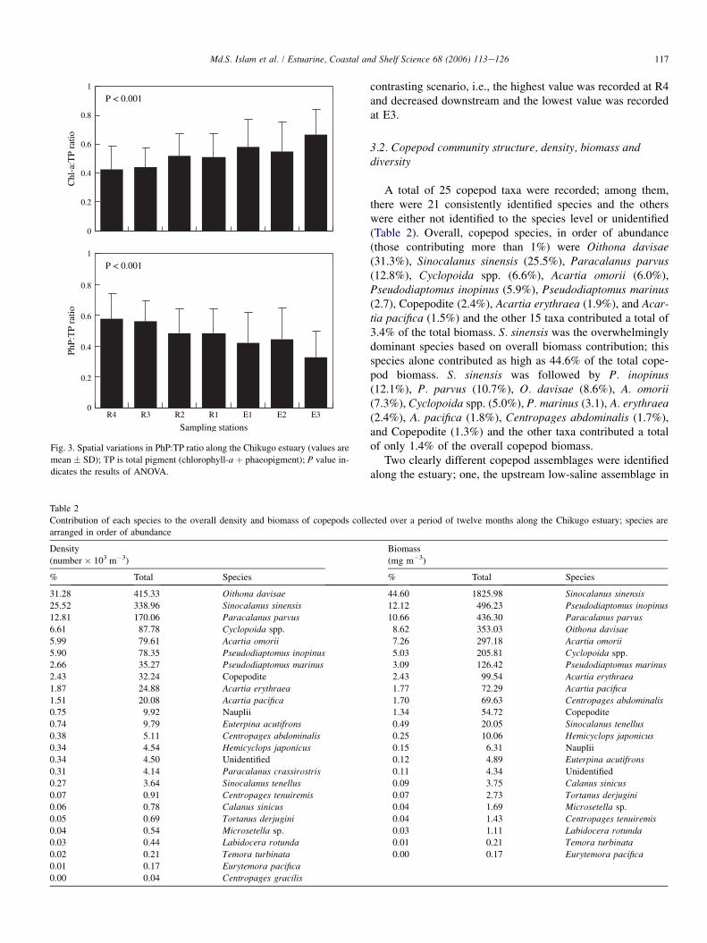
they were calculated as proportion of the total pigment. Theratio of chl-a to total pigment (TP) (chl-a þ PhP) and thatof PhP to TP were calculated as an index of chl-a and PhP pro-duction and their relative contribution to the total pigment overthe spatial scale. Contrary to the chl-a concentrations which

showed no significant spatial variations, chl-a:TP ratio showedsignificant spatial variations (P < 0.001) with the lowest valueat R4 and increased towards downstream and the highest valuewas observed at E3 (Fig. 3). Spatial variations of PhP:TP ratioalso was significant (P < 0.001) and showed a completely

Table 1

Pearson’s correlation coefficient between different hydrographical variables, pigments and copepod density, diversity and biomass collected over the spatio-

temporal scales from the Chikugo estuary (*P < 0.05; **P < 0.01)

Temperature Salinity Turbidity Chl-a PhP Density Biomass

Salinity 0.12 e

Turbidity �0.22* �0.42** e

Chl-a 0.50** �0.08 0.25* ePhP �0.07 �0.49** 0.68** 0.43** e

Density 0.43** 0.08 0.13 0.60** 0.22* e

Biomass 0.26* �0.19 0.39** 0.69** 0.45** 0.82** e

H 0.45** 0.27* �0.20 0.04 �0.20 �0.14 �0.16


0

0.2

0.4

0.6

0.8

1

P < 0.001

Chl

-a:T

P ra

tio

0

0.2

0.4

0.6

0.8

1

R4 R3 R2 R1 E1 E2 E3

P < 0.001

PhP:

TP

ratio

Sampling stations

Fig. 3. Spatial variations in PhP:TP ratio along the Chikugo estuary (values are

mean � SD); TP is total pigment (chlorophyll-a þ phaeopigment); P value in-

dicates the results of ANOVA.

contrasting scenario, i.e., the highest value was recorded at R4and decreased downstream and the lowest value was recordedat E3.

3.2. Copepod community structure, density, biomass anddiversity

A total of 25 copepod taxa were recorded; among them,there were 21 consistently identified species and the otherswere either not identified to the species level or unidentified(Table 2). Overall, copepod species, in order of abundance(those contributing more than 1%) were Oithona davisae(31.3%), Sinocalanus sinensis (25.5%), Paracalanus parvus(12.8%), Cyclopoida spp. (6.6%), Acartia omorii (6.0%),Pseudodiaptomus inopinus (5.9%), Pseudodiaptomus marinus(2.7), Copepodite (2.4%), Acartia erythraea (1.9%), and Acar-tia pacifica (1.5%) and the other 15 taxa contributed a total of3.4% of the total biomass. S. sinensis was the overwhelminglydominant species based on overall biomass contribution; thisspecies alone contributed as high as 44.6% of the total cope-pod biomass. S. sinensis was followed by P. inopinus(12.1%), P. parvus (10.7%), O. davisae (8.6%), A. omorii(7.3%), Cyclopoida spp. (5.0%), P. marinus (3.1), A. erythraea(2.4%), A. pacifica (1.8%), Centropages abdominalis (1.7%),and Copepodite (1.3%) and the other taxa contributed a totalof only 1.4% of the overall copepod biomass.

Two clearly different copepod assemblages were identifiedalong the estuary; one, the upstream low-saline assemblage in

Table 2

Contribution of each species to the overall density and biomass of copepods collected over a period of twelve months along the Chikugo estuary; species are

arranged in order of abundance

Density

(number � 103 m�3)

Biomass

(mg m�3)

% Total Species % Total Species

31.28 415.33 Oithona davisae 44.60 1825.98 Sinocalanus sinensis

25.52 338.96 Sinocalanus sinensis 12.12 496.23 Pseudodiaptomus inopinus

12.81 170.06 Paracalanus parvus 10.66 436.30 Paracalanus parvus6.61 87.78 Cyclopoida spp. 8.62 353.03 Oithona davisae

5.99 79.61 Acartia omorii 7.26 297.18 Acartia omorii

5.90 78.35 Pseudodiaptomus inopinus 5.03 205.81 Cyclopoida spp.

2.66 35.27 Pseudodiaptomus marinus 3.09 126.42 Pseudodiaptomus marinus

2.43 32.24 Copepodite 2.43 99.54 Acartia erythraea

1.87 24.88 Acartia erythraea 1.77 72.29 Acartia pacifica

1.51 20.08 Acartia pacifica 1.70 69.63 Centropages abdominalis0.75 9.92 Nauplii 1.34 54.72 Copepodite

0.74 9.79 Euterpina acutifrons 0.49 20.05 Sinocalanus tenellus

0.38 5.11 Centropages abdominalis 0.25 10.06 Hemicyclops japonicus

0.34 4.54 Hemicyclops japonicus 0.15 6.31 Nauplii

0.34 4.50 Unidentified 0.12 4.89 Euterpina acutifrons

0.31 4.14 Paracalanus crassirostris 0.11 4.34 Unidentified

0.27 3.64 Sinocalanus tenellus 0.09 3.75 Calanus sinicus

0.07 0.91 Centropages tenuiremis 0.07 2.73 Tortanus derjugini0.06 0.78 Calanus sinicus 0.04 1.69 Microsetella sp.

0.05 0.69 Tortanus derjugini 0.04 1.43 Centropages tenuiremis

0.04 0.54 Microsetella sp. 0.03 1.11 Labidocera rotunda0.03 0.44 Labidocera rotunda 0.01 0.21 Temora turbinata

0.02 0.21 Temora turbinata 0.00 0.17 Eurytemora pacifica

0.01 0.17 Eurytemora pacifica

0.00 0.04 Centropages gracilis


0%

25%

50%

75%

100%

0%

25%

50%

75%

100%

1.0 4.1 15.6 22.6 25.6 27.7 29.20%

25%

50%

75%

100%

0.2 1.1 7.7 13.0 15.1 22.6 26.0

0%

25%

50%

75%

100%

0 0 0.1 0.6 2.3 10.1 10.2 0.4 2.0 10.1 16.1 16.5 22.6 27.1

0%

25%

50%

75%

100%

0%

25%

50%

75%

100%

0%

25%

50%

75%

100%

0%

25%

50%

75%

100%

0%

25%

50%

75%

100%

1.9 11.0 20.3 25.2 26.9 28.3 30.1 0.2 1.2 9.2 18.5 18.6 21.8 26.3

0%

25%

50%

75%

100%

0.2 1.6 8.6 16.7 17.7 19.0 23.2 0.6 5.4 15.6 21.7 23.5 25.1 27.0

0%

25%

50%

75%

100%

2.0 3.7 11.8 17.7 21.3 22.9 28.5 0.1 0.5 4.3 11.4 16.7 20.0 25.0

0%

25%

50%

75%

100%

0.1 0.2 5.0 11.7 13.3 20.5 22.3 0.1 0.1 0.6 6.0 9.8 16.5 24.0

A

M

J

J

S

O

A

N

D

J

F

M

Cop

epod

spe

cies

com

posi

tion

(den

sity

, %)

Salinity Salinity

Acartia omorii

Acartia pacificaCentropages abdominalis

Acartia erythraea

CopepoditeCentropages tenuiremis

Calanus sinicus

Cyclopoida sp.

Euterpina acutifrons

Hemicyclops japonicus

Labidocera rotunda

Microsetella sp.

Copepod nauplii

Oithona davisae

Pseudodiaptomus inopinus

Pseudodiaptomus marinus

Paracalanus parvus

Paracalanus crassirostris

Sinocalanus sinensis

Sinocalanus tenellus

Tortanus derjuginiUnidentified

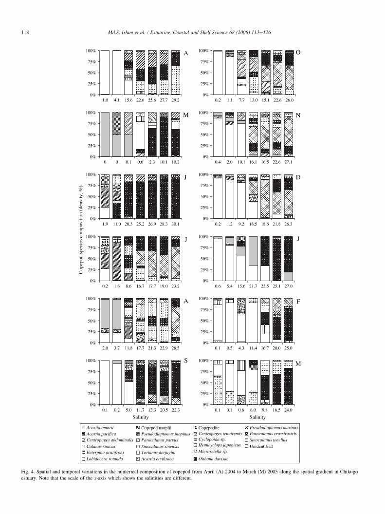
Fig. 4. Spatial and temporal variations in the numerical composition of copepod from April (A) 2004 to March (M) 2005 along the spatial gradient in Chikugo

estuary. Note that the scale of the x-axis which shows the salinities are different.


station R4eR2 (extended down to R1 during winter) and, theother, the high salinity assemblage in station R1eE3. The lowsalinity assemblage was dominated by only a few species,mainly S. sinensis during almost the whole survey period(Fig. 4). Exception occurs during MayeAugust when Cyclo-poida spp. and P. inopinus dominated. In contrast, the high sa-linity downstream assemblage was dominated by a number ofspecies which were seasonally variable. Major species of thisassemblage were O. davisae, P. parvus, A. omorii, P. marinusand some other common coastal copepods. O. davisaedominated overwhelmingly during May, June, Septemberand January and P. parvus in July and from October toDecember. A. omorii dominated during FebruaryeMarch; inApril, A. omorii, O. davisae and P. marinus co-occurred andcontributed almost equally.

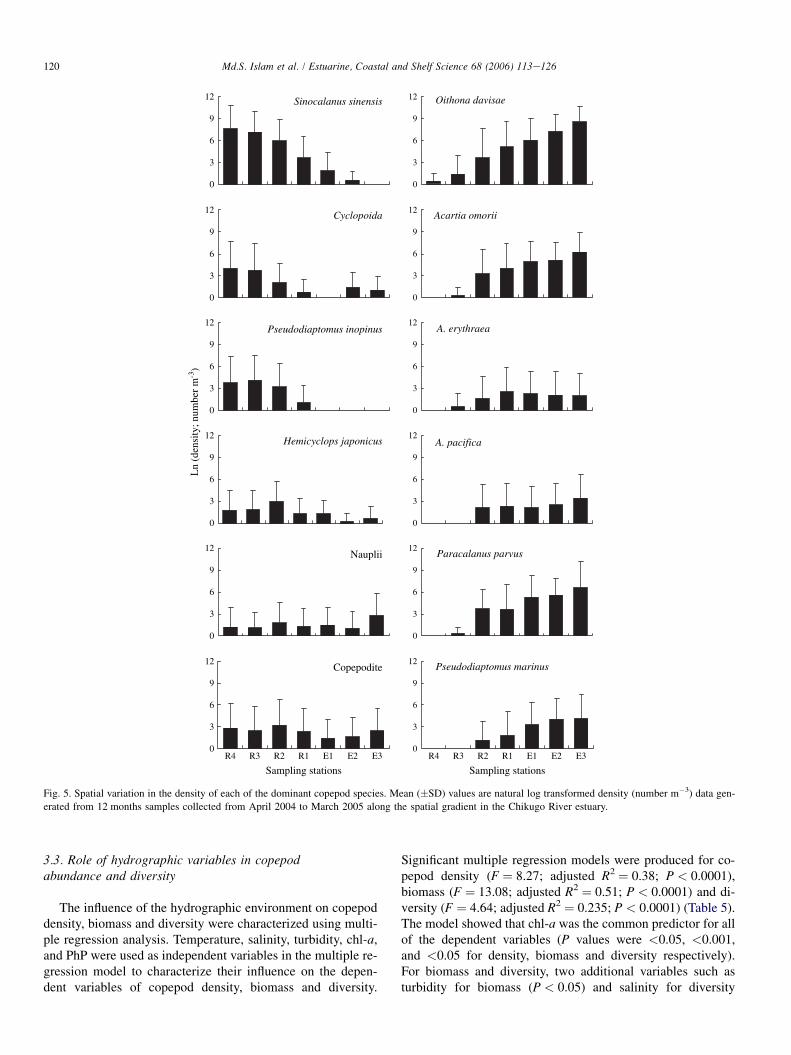
Spatio-temporal variations of most of the dominant cope-pods were significant (Table 3). There were three groups basedon spatial distribution: (1) those showing significantly (Table 3)higher density in the upper estuary (S. sinensis, Cyclopoida,P. inopinus and H. japonicus), (2) those showing no significantspatial variation and (3) those showing significantly higherdensity in the lower estuary (O. davisae, A. omorii, A. eryth-raea, A. pacifica, P. parvus, P. marinus) (Fig. 5). Monthly var-iations in the abundance of dominant species showed that mostof the dominant species were generally highly abundant duringJuneeAugust (Fig. 6), corresponding with the periods of hightemperature. Thus, the monthly abundance of A. erythraea,A. pacifica, Copepodite, P. inopinus, P. marinus, and H. japo-nicus correlated significantly with the monthly patterns oftemperature and chl-a (Table 4). In contrast, S. sinensis,

Table 3

Two-way analysis of variance (ANOVA) summary results of the spatial (seven

sampling stations) and temporal (12 months) variations in the density of the

dominant copepod species along the Chikugo estuary

Copepod species Sources of

variation

df F P

Cyclopoida sp. Temporal 11 5.21 0.000

Spatial 6 7.02 0.000

Sinocalanus sinensis Temporal 11 1.90 0.055

Spatial 6 21.76 0.000

Nauplii Temporal 11 2.42 0.013

Spatial 6 0.82 0.556

Acartia omorii Temporal 11 5.08 0.000

Spatial 6 17.49 0.000

Hemicyclops japonicus Temporal 11 2.61 0.008

Spatial 6 2.30 0.045

Oithona davisae Temporal 11 5.61 0.000

Spatial 6 23.61 0.000

Pseudodiaptomus inopinus Temporal 11 3.34 0.001

Spatial 6 10.00 0.000

Pseudodiaptomus marinus Temporal 11 4.89 0.000

Spatial 6 8.87 0.000

Paracalanus parvus Temporal 11 5.97 0.000

Spatial 6 20.30 0.000

Copepodite Temporal 11 3.98 0.000

Spatial 6 0.73 0.626

Acartia erythraea Temporal 11 8.51 0.000

Spatial 6 2.98 0.012

Acartia pacifica Temporal 11 9.00 0.000

Spatial 6 6.67 0.000

O. davisae, P. parvus, A. omorii, copepod nauplii and Cyclo-poida spp. did not show consistent monthly patterns andwere not correlated with monthly temperature variationsalthough temporal variations in the density of these copepodswere significant. The dominant species in the two contrastingcopepod communities showed a completely contrasting spatialdistribution pattern in their density. Copepods of the low salineupstream assemblage (S. sinensis and P. inopinus) showeda decrease in abundance towards downstream while those ofthe high saline marine assemblage (O. davisae, P. parvus,Acartia spp. and P. marinus) showed an increase in abundancetoward the sea (Fig. 7).

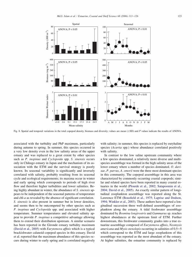
Copepod density showed significant spatial variations(P < 0.05) with the highest mean density of (32.6 �39.7) � 103 m�3 at E3 and the lowest mean density of(7.9 � 10.3) � 103 m�3 at R2. There were three major spatialzones based on copepod density; a high density zone in thelower estuary (E2eE3), a medium density zone in the upperestuary (R4eR3) and a low density zone in between (R2eE1) (Fig. 8). In contrast to copepod density, the highest stand-ing biomass of 121.6 � 217.6 mg m�3 was recorded at the up-permost station and the lowest value of 18.5 � 20.0 mg m�3

was recorded at R1 and varied significantly between stations(P < 0.05). Similar to copepod density, there were three majorspatial zones based on copepod standing biomass. However,in contrast to the density patterns, the zone of high biomassoccurred in the upper estuary (R4eR3), the zone of mediumbiomass in the lower estuary (E2eE3) and the zone of lowbiomass in between (R2eE1). Copepod density and standingbiomass showed significant (P < 0.005 and P < 0.05 respec-tively) temporal variations; higher density and biomass wereobserved during AprileSeptember (except for May). Therewere two distinct regions based on all the indexes of diversityused. The upper estuary (R4eR3) had significantly lower di-versity than the lower estuary (R2eE3) and this pattern wasconsistent with the ShannoneWeiner index (P < 0.001), spe-cies richness (P < 0.05) and evenness (P < 0.01). The highestvalues of all the indexes were observed at R2 and the lowestvalue at R4.

Table 4

Relationships (Pearson’s correlation coefficient) between the monthly patterns

of temperature and chl-a and the monthly abundance of dominant species of

copepods (**P < 0.01; *P < 0.05)

Species Temperature Chl-a

S. sinensis �0.01 0.39

O. davisae 0.44 0.28

A. omorii 0.38 0.68*

Cyclopoida spp. 0.46 0.48

Nauplii 0.41 0.16

C. abdominalis 0.17 0.01

P. parvus 0.47 0.41

P. inopinus 0.62* 0.60*

P. marinus 0.64* 0.72**

A. erythraea 0.69* 0.66*

A. pacifica 0.74** 0.66*

H. japonicus 0.76** 0.68*

Copepodite 0.74** 0.54



0

3

6

9

12 Oithona davisae

0

3

6

9

12

Cyclopoida

0

3

6

9

12 Acartia omorii

0

3

6

9

12


0

3

6

9

12A. erythraea

0

3

6

9

12


0

3

6

9

12A. pacifica

0

3

6

9

12

Nauplii

0

3

6

9

12Paracalanus parvus

0

3

6

9

12

Copepodite

0

3

6

9

12

R4 R3 R2 R1 E1 E2 E3


0

3

6

9

12

R4 R3 R2 R1 E1 E2 E3

Sampling stationsSampling stations

Ln

(den

sity

; num

ber

m-3

)

Fig. 5. Spatial variation in the density of each of the dominant copepod species. Mean (�SD) values are natural log transformed density (number m�3) data gen-

erated from 12 months samples collected from April 2004 to March 2005 along the spatial gradient in the Chikugo River estuary.

3.3. Role of hydrographic variables in copepodabundance and diversity

The influence of the hydrographic environment on copepoddensity, biomass and diversity were characterized using multi-ple regression analysis. Temperature, salinity, turbidity, chl-a,and PhP were used as independent variables in the multiple re-gression model to characterize their influence on the depen-dent variables of copepod density, biomass and diversity.

Significant multiple regression models were produced for co-pepod density (F ¼ 8.27; adjusted R2 ¼ 0.38; P < 0.0001),biomass (F ¼ 13.08; adjusted R2 ¼ 0.51; P < 0.0001) and di-versity (F ¼ 4.64; adjusted R2 ¼ 0.235; P < 0.0001) (Table 5).The model showed that chl-a was the common predictor for allof the dependent variables (P values were <0.05, <0.001,and <0.05 for density, biomass and diversity respectively).For biomass and diversity, two additional variables such asturbidity for biomass (P < 0.05) and salinity for diversity


Acartia erythraea9

12

Acartia omorii9

12

0

3

6

0

3

6

Acartia pacifica

0

3

6

9

12

Nauplii

0

3

6

9

12


0

3

6

9

12

Cyclopoida sp.

0

3

6

9

12


0

3

6

9

12

Paracalanus parvus

0

3

6

9

12

Copepodite

0

3

6

9

12

Oithona davisae0

3

6

9

12


0

3

6

9

12

A J A O D F


0

3

6

9

12

Months Months

Ln

(den

sity

; num

ber

m-3

)

M J S N J M A J A O D FM J S N J M

Fig. 6. Temporal variation in the density of each of the dominant copepods. Values are natural log transformed density (number m�3) collected from April 2004 to

March 2005 along the spatial gradient in the Chikugo River estuary.

(P < 0.05) were found as significant predictors. The environ-mental parameters and copepod density, biomass and diversitywere calculated separately for four main seasons, i.e.,winter (DecembereFebruary), spring (MarcheMay), summer(JuneeAugust) and autumn (SeptembereNovember) andthe Pearson’s correlation analysis was performed to examinethe relationships among the variables. Only temperature,chl-a and copepod density showed significant correlations(Fig. 9). When multiple regressions were done using each

dominant species as the dependent variable, only the twomost dominant species such as S. sinensis (F ¼ 4.95; adjustedR2 ¼ 0.74; P < 0.05) and O. davisae (F ¼ 6.54; adjustedR2 ¼ 0.801; P < 0.05) produced significant models. Again,chl-a was the significant common predictor variable for bothS. sinensis (P < 0.05) and O. davisae (P < 0.05) and oneadditional variable such as PhP (P < 0.05) was significantpredictor for S. sinensis. Multiple regression models with theother species were not significant, suggesting that either the


0

5

10

15

0

5

10

15

0

5

10

15

0

5

10

15

0

5

10

15

0

5

10

15

<1.0 2.6 9.1 15.1 17.3 21.4 24.9

Oithona davisae

Acartia omorii

Paracalanus parvus




Mean salinity

Ln

(den

sity

; num

ber

m-3

)

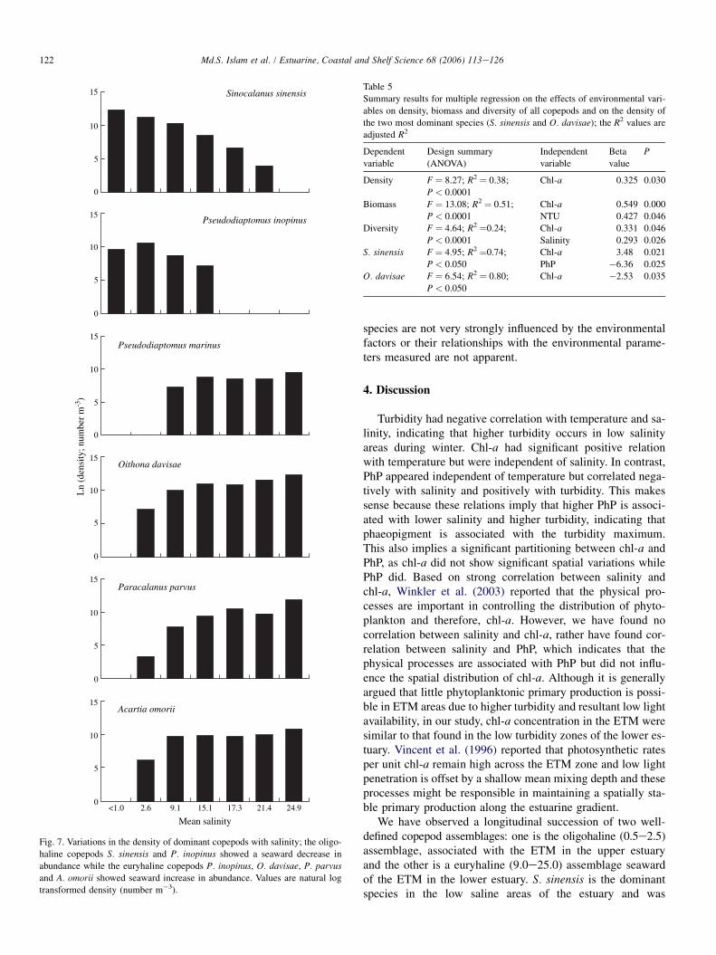
Fig. 7. Variations in the density of dominant copepods with salinity; the oligo-

haline copepods S. sinensis and P. inopinus showed a seaward decrease in

abundance while the euryhaline copepods P. inopinus, O. davisae, P. parvus

and A. omorii showed seaward increase in abundance. Values are natural log

transformed density (number m�3).

species are not very strongly influenced by the environmentalfactors or their relationships with the environmental parame-ters measured are not apparent.

4. Discussion

Turbidity had negative correlation with temperature and sa-linity, indicating that higher turbidity occurs in low salinityareas during winter. Chl-a had significant positive relationwith temperature but were independent of salinity. In contrast,PhP appeared independent of temperature but correlated nega-tively with salinity and positively with turbidity. This makessense because these relations imply that higher PhP is associ-ated with lower salinity and higher turbidity, indicating thatphaeopigment is associated with the turbidity maximum.This also implies a significant partitioning between chl-a andPhP, as chl-a did not show significant spatial variations whilePhP did. Based on strong correlation between salinity andchl-a, Winkler et al. (2003) reported that the physical pro-cesses are important in controlling the distribution of phyto-plankton and therefore, chl-a. However, we have found nocorrelation between salinity and chl-a, rather have found cor-relation between salinity and PhP, which indicates that thephysical processes are associated with PhP but did not influ-ence the spatial distribution of chl-a. Although it is generallyargued that little phytoplanktonic primary production is possi-ble in ETM areas due to higher turbidity and resultant low lightavailability, in our study, chl-a concentration in the ETM weresimilar to that found in the low turbidity zones of the lower es-tuary. Vincent et al. (1996) reported that photosynthetic ratesper unit chl-a remain high across the ETM zone and low lightpenetration is offset by a shallow mean mixing depth and theseprocesses might be responsible in maintaining a spatially sta-ble primary production along the estuarine gradient.

We have observed a longitudinal succession of two well-defined copepod assemblages: one is the oligohaline (0.5e2.5)assemblage, associated with the ETM in the upper estuaryand the other is a euryhaline (9.0e25.0) assemblage seawardof the ETM in the lower estuary. S. sinensis is the dominantspecies in the low saline areas of the estuary and was

Table 5

Summary results for multiple regression on the effects of environmental vari-

ables on density, biomass and diversity of all copepods and on the density of

the two most dominant species (S. sinensis and O. davisae); the R2 values are

adjusted R2

Dependent

variable

Design summary

(ANOVA)

Independent

variable

Beta

value

P

Density F ¼ 8.27; R2 ¼ 0.38;

P < 0.0001

Chl-a 0.325 0.030

Biomass F ¼ 13.08; R2 ¼ 0.51;

P < 0.0001

Chl-a 0.549 0.000

NTU 0.427 0.046

Diversity F ¼ 4.64; R2 ¼0.24;

P < 0.0001

Chl-a 0.331 0.046

Salinity 0.293 0.026

S. sinensis F ¼ 4.95; R2 ¼0.74;

P < 0.050

Chl-a 3.48 0.021

PhP �6.36 0.025

O. davisae F ¼ 6.54; R2 ¼ 0.80;

P < 0.050

Chl-a �2.53 0.035


0

20

40

60

80

0

20

40

60

80

100

0

80

160

240

320

400

0

100

200

300

400

500

0

1

2

3

<1.0 2.6 9.1 15.1 17.3 21.4 24.90

1

2

3

A M J J A S O N D J F M

ANOVA; P < 0.05

ANOVA; P < 0.05 ANOVA; P < 0.05

ANOVA; P < 0.01 ANOVA; P < 0.01

Mean salinity Months

Spatial Seasonal

ANOVA; P < 0.01

Den

sity

(,0

00 m

-3)

Bio

mas

s (m

g m

-3)

Shan

non-

Wei

ner

inde

x

Fig. 8. Spatial and temporal variations in the total copepod density, biomass and diversity; values are mean (�SD) and P values indicate the results of ANOVA.

associated with the turbidity and PhP maximum, particularlyduring autumn to spring. In summer, this species occurred ina very low density even in the low salinity areas of the upperestuary and was replaced to a great extent by other speciessuch as P. inopinus and Cyclopoida spp. S. sinensis occursonly in Chikugo estuary in Japan and the mechanism of its as-sociation with the ETM and the survival strategy is poorlyknown. Its seasonal variability is significantly and inverselycorrelated with salinity, probably resulting from its seasonalcycle and ecological requirements; its maxima occur in winterand early spring which corresponds to periods of high riverflow and therefore higher turbidities and lower salinities. Be-ing highly abundant in winter, the abundance of S. sinensis ap-pears to be independent of the seasonal patterns of temperatureand chl-a as revealed by the absence of significant correlation.S. sinensis is also present in summer but in lower densities,and seems then to be outcompeted by other species such asP. inopinus and Cyclopoida spp. and associated with highertemperature. Summer temperatures and elevated salinity ap-pear to provide P. inopinus a competitive advantage allowingthem to extend their distribution upstream. A similar scenariohas been reported in the Gironde estuary turbidity maximum(David et al., 2005) with Eurytemora affinis which is a typicalbrackishwater calanoid copepod species in this estuary. Davidet al. reported that the maximum abundance of this species oc-curs during winter to early spring and is correlated negatively

with salinity; in summer, this species is replaced by euryhalinespecies (Acartia spp.) whose abundance correlated positivelywith salinity.

In contrast to the low saline upstream community wherea few species dominated, a relatively more diverse and multi-species assemblage was formed in the high salinity areas of thelower estuary where a number of species dominated. O. davi-sae, P. parvus, A. omorii were the three most dominant speciesin this community. The copepod assemblage in this area wascharacterized by commonly occurring coastal copepods; simi-lar and related species have been reported in many coastal es-tuaries in the world (Plourde et al., 2002; Satapoomin et al.,2004; David et al., 2005). An exactly similar pattern of longi-tudinal zooplankton assemblage was reported along the St.Lawrence ETM (Bousfield et al., 1975; Laprise and Dodson,1994; Winkler et al., 2003). These authors have reported a lon-gitudinal succession three well-defined assemblages of zoo-plankton along the estuary. A tidal freshwater assemblagedominated by Bosmina longirostris and Gammarus sp. reacheshighest abundances at the upstream limit of ETM. Furtherdownstream, this freshwater community grades into a true es-tuarine assemblage composed of Eurytemora affinis, Neomysisamericana and Mysis stenolepis occurring in salinities of 0.5e5which correspond to the ETM and large zooplankton of thisassemblage was reported as the most abundant of the estuary.At higher salinities, the estuarine community is replaced by


a euryhaline marine assemblage composed of Calanus spp.and other commonly occurring coastal marine zooplanktons(Bousfield et al., 1975; Laprise and Dodson, 1994).

Similar to S. sinensis in the upper estuary, the dominant spe-cies in the lower estuary (O. davisae, P. parvus, A. omorii, Cy-clopoida spp.) did not show significant relation with monthlytemperature cycle. In contrast, most of the medium abundantspecies (A. erythraea, A. pacifica, P. marinus, H. japonicus)showed generally high abundance during the summer monthsand had highly significant correlation with temperature andchl-a, indicating that production of these species depends onseasonal cycle of temperature and is, therefore, associatedwith active primary production by phytoplankton. Therefore,there were two major categories of copepod assemblages basedon seasonal abundance patterns: the first category comprised ofhighly abundant and dominant species which are independentof seasonal temperature cycle (S. sinensis in the upper andO. davisae, P. parvus and A. omorii in the lower estuary) andthe second category includes the medium abundant speciesthat are dependent on seasonal temperature cycle and are

0

8

16

24

32

0

4

8

12

16

0

50

100

150

200

250

300

Winter Spring Summer Autumn

Tem

pera

ture

Chl

orop

hyll-

aC

opep

od d

ensi

ty

Fig. 9. Patterns of interrelationships among temperature ( �C), chl-a (mg l�1)

and copepod density (number m�3) during four main seasons. Values are

mean and error bars are standard deviations of three samples during each sea-

son. Pearson’s correlation coefficient showed that seasonal patterns in temper-

ature, chl-a and density were significantly related to each other (values or r

were 0.917 (P < 0.05), 0.921 (P < 0.05) and 0.997 (P < 0.01) for temperature

vs chl-a, temperature vs density and chl-a vs density respectively.

associated with high summer temperature (P. inopinus in theupper and A. erythraea, A. pacifica, P. marinus, H. japonicusin the lower estuary). The highest total copepod density oc-curred at E3, the most downstream station; in contrast, thehighest standing biomass occurred at R4, the most upstreamstation, indicating that S. sinensis accounts for most of the sec-ondary production by copepods in the estuary. As a single spe-cies, S. sinensis, which is associated with the ETM zone of theestuary contributed as high as 44.6% of the overall copepod bio-mass production and, in association with P. inopinus, which isalso associated with ETM, contributed 56.7% of the total cope-pod standing biomass in the estuary. This implies that the ETMzone accounts for majority of the copepod biomass productionand is consistent with other well mixed estuarine systems thatare characterized by an ETM zone (Laprise and Dodson, 1994;Winkler et al., 2003). Both density and biomass showed highervalues during the summer period and had significant correla-tion with temperature, chl-a and PhP; this implies that the sea-sonal cycle in pigment production, which is influenced byseasonal temperature patterns, plays an important role in cope-pod abundance and biomass production in the estuary (Kiorboeand Nielsen, 1994).

Abundance of S. sinensis and P. inopinus, which aremembers of the low saline upstream assemblage, decreasedsharply toward the sea in contrast to the abundance of thedominant species of the low saline marine communitywhich showed sharp upstream decrease. This contrastingspatial abundance pattern explains the habitat partitioningbetween these two communities. This implies that themain habitats of the copepods of the upstream assemblageare associated with the low salinity waters flowing and car-rying them downstream while habitats of the euryhaline ma-rine species are formed in more saline deep waters flowingand carrying them upstream, suggesting that animals may beconfined in waters that transport them away from the cen-ters of their respective populations. We, therefore, speculatethat the original habitat of the oligohaline community is lo-cated towards more upstream and that of the euryhalinecommunity towards more downstream because the highestdensity of the two communities occurred at the two endsof the gradient. This pattern is in strong agreement withthat reported by Bousfield et al. (1975) and Dodson et al.(1989). Bousfield et al. (1975) suggested that the copepodsthat are transported from their original habitats are mostlymoribund, non-reproductive animals, suggesting that thetransported habitats may constitute an extreme environmentfor these species. Consequently, lowest copepod abundancesare obtainable in areas between the original low salineupstream estuarine assemblage and euryhaline downstreammarine assemblage. In contrast, the edge effects, causedby mixing individuals from the two assemblages, result inincreasing the species richness. Therefore, species richnessmay give erroneous impressions on the evolution of cope-pod species diversity along the spatial gradient in an estuary(Laprise and Dodson, 1994).

Chl-a was found as the common and the most importantpredictor variable for total copepod density, biomass and


diversity as well as the density of dominant species. Salinity,by virtue of its spatial differences, was a significant predictorof the diversity estimates; this was expected because higher di-versity was recorded in the higher salinity regions. Chl-a wasfound as a significant predictor for O. davisae, indicating thatthe abundance of O. davisae is dependent on primary produc-tion by phytoplankton and is presumably independent of PhP.In contrast, PhP was an additional variable for S. sinensis,which indicates that the abundance of S. sinensis is controlledto a significant extent by the supply of phaeopigment sources.Therefore, chl-a is the most important variable that can de-scribe the observed variability in copepod density, biomassand diversity in the estuary as a whole, and PhP is the addi-tional variable for copepods in the upper estuary alone. Similarscenarios are reported in other comparable ecosystems such asin the Gironde estuary (Irigoien and Castel, 1997; David et al.,2005), the St. Lawrence River estuary (Winkler et al., 2003),and in Chesapeake Bay turbidity maximum (Roman et al.,2001). High turbidities alter the nutritional environment andthus affect feeding, survival and reproduction of the copepodspecies residing in the ETM areas. As a consequence, the co-pepod populations of ETM zones are mainly localized as a re-sult of hydrodynamic processes. In contrast, O. davisae andAcartia spp. that are dominant copepod species seaward ofthe maximum turbidity area were distributed preferentiallydownstream, illustrating their greater tolerance to higher salin-ity. Similar distribution patterns were reported by David et al.(2005) in the Gironde estuary. They reported that a calanoidcopepod Eurytemora affinis was restrictedly distributed inthe turbidity maximum area while Acartia spp. were distrib-uted toward the downstream areas. However, copepod speciesassemblages are not simply the result of species sorting inde-pendently according to their salinity tolerance and, as in someother studies (Laprise and Dodson, 1994), our results supportthe hypothesis that environmental variability is a major factorinfluencing distribution and species diversity of copepod inestuaries.

Acknowledgements

This research was supported by a research grant providedby the Japanese Government Ministry of Education, Culture,Sports, Science and Technology (Monbukagakusho, MEXT)and the first author acknowledges the financial support pro-vided by the ‘Monbukagakusho’ (through ‘MonbukagakushoScholarship’) during his stay in Japan. We thank the graduatestudents of Division of Applied Biosciences, Kyoto Universityfor their assistance in field samplings.

References

Berasategui, A.D., Ramı́rez, F.C., Schiariti, A., 2005. Patterns in diversity and

community structure of epipelagic copepods from the BrazileMalvinas

Confluence area, south-western Atlantic. Journal of Marine Systems 56,

309e316.

Beyst, B., Buysse, D., Dewicke, A., Mees, J., 2001. Surf zone hyperbenthos of

Belgian sandy beaches: seasonal patterns. Estuarine, Coastal and Shelf Sci-

ence 53, 877e895.

Bousfield, E.L., Filteau, G., O’Neill, M., Gentes, P., 1975. Population dynam-

ics of zooplankton in the middle St. Lawrence estuary. Estuarine Research

1, 325e351.

Christou, E.D., 1998. Interannual variability of copepods in a Mediterranean

coastal area (Saronikos Gulf, Aegean Sea). Journal of Marine Systems

15, 523e532.

David, V., Sautour, B., Chardy, P., Leconte, M., 2005. Long-term changes of

the zooplankton variability in a turbid environment: the Gironde estuary

(France). Estuarine, Coastal and Shelf Science 64, 171e184.

Dodson, J.J., Dauvin, J.C., Ingram, R.G., d’Anglejan, B., 1989. Abundance of

larval rainbow smelt (Osmerus mordax) in relation to the maximum turbid-

ity zone and associated macroplankton fauna of the middle St. Lawrence

estuary. Estuaries 12, 66e81.

Durbin, A.G., Durbin, E.G., 1981. Standing stock and estimated production

rates of phytoplankton and zooplankton in Narragansett Bay, Rhode Island.

Estuaries 4, 24e41.

Escribano, R., Hidalgo, P., 2000. Spatial distribution of copepods in the

North of the Humboldt Current region off Chile during coastal upwelling.

Journal of Marine Biological Association of the United Kingdom 80,

283e290.

Gasparini, S., Castel, J., Irigoien, X., 1999. Impact of suspended particulate

matter on egg production of the estuarine copepod, Eurytemora affinis.

Journal of Marine Systems 22, 195e205.

Hassel, A., 1986. Seasonal changes in zooplankton composition in the Barents

Sea, with special attention to Calanus spp. (Copepoda). Journal of Plank-

ton Research 8, 329e339.

Irigoien, X., Castel, J., 1997. Light limitation and distribution of chlorophyll

pigments in a highly turbid estuary: the Gironde (SW France). Estuarine,

Coastal and Shelf Science 44, 507e517.

Islam, M.S., Ueda, H., Tanaka, M., 2004. Spatial distribution and trophic ecol-

ogy of dominant copepods associated with turbidity maximum along the

salinity gradient and in a highly embayed estuarine system in Ariake

Sea, Japan. Journal of Experimental Marine Biology and Ecology 316,

101e115.

Kimmerer, W.J., Burau, J.R., Bennet, W.A., 1998. Tidally oriented vertical mi-

gration and position maintenance of zooplankton in a temperate estuary.

Limnology and Oceanography 43, 1697e1709.

Kiorboe, T., Nielsen, T.G., 1994. Regulation of zooplankton biomass and pro-

duction in a temperate, coastal ecosystem. 1. Copepods. Limnology and

Oceanography 39, 493e507.

Laprise, R., Dodson, J.J., 1994. Environmental variability as a factor control-

ling spatial patterns in distribution and species diversity of zooplankton in

the St. Lawrence estuary. Marine Ecology Progress Series 107, 67e81.

Lawrence, D., Valiela, I., Tomasky, G., 2004. Estuarine calanoid copepod

abundance in relation to season, salinity, and land-derived nitrogen load-

ing, Waquoit Bay, MA. Estuarine, Coastal and Shelf Science 61, 547e557.

MacKenzie, B.R., Kiørboe, T., 2000. Larval fish feeding and turbulence: a case

for the downside. Limnology and Oceanography 45, 1e10.

MacKenzie, B.R., Miller, T.J., Cyr, S., Leggett, W.C., 1994. Evidence for

a dome-shaped relationship between turbulence and larval fish ingestion

rates. Limnology and Oceanography 39, 1790e1799.

Manning, C.A., Bucklin, A., 2005. Multivariate analysis of the copepod com-

munity of near-shore waters in the western Gulf of Maine. Marine Ecology

Progress Series 292, 233e249.

Plourde, S., Dodson, J.J., Runge, J.A., Therriault, J.C., 2002. Spatial

and temporal variations in copepod community structure in the lower

St. Lawrence Estuary, Canada. Marine Ecology Progress Series 230,

211e224.

Roddie, B.D., Leakey, R.J.G., Berry, A.J., 1984. Salinityetemperature

tolerance and osmoregulation in Eurytemora affinis (Poppe) (Copepoda:

Calanoida) in relation to its distribution in the zooplankton of the upper

reaches of the Fourth estuary. Journal of Experimental Marine Biology

Ecology 79, 191e211.

Roff, J.C., Middlebrook, K., Evans, F., 1988. Long-term variability in North

Sea zooplankton off Northumberland coast: productivity of small copepods


and analysis of trophic interactions. Journal of the Marine Biological

Association of the United Kingdom 68, 143e164.

Roman, M.R., Holliday, D.V., Sanford, L.P., 2001. Temporal and spatial

patterns of zooplankton in the Chesapeake Bay turbidity maximum.

Marine Ecology Progress Series 213, 215e227.

Rothschild, B.J., Osborn, T.R., 1988. Small scale turbulence and plankton

contact rates. Journal of Plankton Research 10, 465e474.

Satapoomin, S., Nielsen, T.G., Hansen, P.J., 2004. Andaman Sea cope-

pods: spatio-temporal variations in biomass and production, and role

in the pelagic food web. Marine Ecology Progress Series 274,

99e122.

Underwood, A.J., 1997. Experiments in Ecology: Their Logical Design and Inter-

pretation Using Analysis of Variances. Cambridge University Press, Cambridge.

Vincent, W.F., Dodson, J.J., Bertrand, N., Frenette, J.J., 1996. Photosynthetic

and bacterial production gradients in a larval fish nursery: the St. Lawrence

River transition zone. Marine Ecology Progress Series 139, 227e238.

Visser, A.W., Saito, H., Saiz, E., Kiørboe, T., 2001. Observations of copepod

feeding and vertical distribution under natural turbulent conditions in the

North Sea. Marine Biology 138, 1011e1019.

Winkler, G., Dodson, J.J., Bertrand, N., Thivierge, D., Vincent, W.F., 2003.

Trophic coupling across the St. Lawrence River estuarine transition

zone. Marine Ecology Progress Series 251, 59e73.

spatial and seasonal variations in copepod communities related to turbidity maximum along the...

Documents