sparse regression and support recovery with l2-boosting algorithms

Journal of Statistical Planning and Inference 155 (2014) 19–41

Contents lists available at ScienceDirect

Journal of Statistical Planning and Inference

journal homepage: www.elsevier.com/locate/jspi

Sparse regression and support recovery with L2-BoostingalgorithmsMagali Champion a,b, Christine Cierco-Ayrolles b, Sébastien Gadat a,∗,Matthieu Vignes b

a Institut de Mathématiques de Toulouse, Université Paul Sabatier, 118 Route de Narbonne, 31062 Toulouse, Cedex 9, Franceb INRA, UR875 MIA-T, F-31326 Castanet-Tolosan, France

a r t i c l e i n f o

Article history:Received 22 February 2013Received in revised form 14 April 2014Accepted 7 July 2014Available online 15 July 2014

Keywords:BoostingRegressionSparsityHigh-dimension

a b s t r a c t

This paper focuses on the analysis of L2-Boosting algorithms for linear regressions. Consis-tency results were obtained for high-dimensional models when the number of predictorsgrows exponentially with the sample size n. We propose a new result for Weak Greedy Al-gorithms that deals with the support recovery, provided that reasonable assumptions onthe regression parameter are fulfilled. For the sake of clarity, we also present some resultsin the deterministic case. Finally, we propose two multi-task versions of L2-Boosting forwhich we can extend these stability results, provided that assumptions on the restrictedisometry of the representation and on the sparsity of the model are fulfilled. The interestof these two algorithms is demonstrated on various datasets.

© 2014 Elsevier B.V. All rights reserved.

1. Introduction

Context of our work

This paper presents a study ofWeak Greedy Algorithms (WGA) and statistical L2-Boosting procedures derived from theseWGA. These methods are dedicated to the approximation or estimation of several parameters that encode the relationshipsbetween input variables X and any response Y through a noisy linear representation Y = f (X) + ε, where ε models theamount of noise in the data. We assume that f may be linearly spanned on a predefined dictionary of functions (gj)j=1...p:

f (x) =

pj=1

ajgj(x). (1)

We aim at recovering unknown coefficients (aj)j=1...p when one n-sample (Xk, Yk)k=1...n is observed in the high-dimensionalparadigm. Moreover, we are also interested in extending the boosting methods to the multi-task situation described inHastie et al. (2009): Y is described by m coordinates Y = (Y 1, . . . , Ym), and each one is modelled by a linear relationshipY i

= f i(X) + εi. These relationships are now parametrised through the family of unknown coefficients (ai,j)1≤i≤m,1≤j≤p.In both univariate or multivariate situations, we are primarily interested in the recovery of the structure (i.e. non-zeroelements) of the matrix A = (ai,j)1≤i≤m,1≤j≤p, when a limited amount of observations n is available compared to the largedimension p of the feature space. In brief, the goal is to identify significant relationships between variables X and Y . Weformulate this paradigmas a feature selection problem:we seek relevant elements of the dictionary (gj(X))j=1...p that explain(in)dependencies in a measured dataset.

∗ Corresponding author.E-mail addresses: [email protected] (M. Champion), [email protected] (C. Cierco-Ayrolles),

[email protected], [email protected] (S. Gadat), [email protected] (M. Vignes).

http://dx.doi.org/10.1016/j.jspi.2014.07.0060378-3758/© 2014 Elsevier B.V. All rights reserved.

http://dx.doi.org/10.1016/j.jspi.2014.07.006

http://www.elsevier.com/locate/jspi

http://www.elsevier.com/locate/jspi

http://crossmark.crossref.org/dialog/?doi=10.1016/j.jspi.2014.07.006&domain=pdf

mailto:[email protected]





http://dx.doi.org/10.1016/j.jspi.2014.07.006

20 M. Champion et al. / Journal of Statistical Planning and Inference 155 (2014) 19–41

Feature selection algorithms can be split into three large families: exhaustive subset exploration, subspacemethods, andforward algorithmswith shrinkage. The exhaustive search suffers fromanobvious hard combinatorial problem (seeHocking,1983), and subspace methods such as (Gadat, 2008) are generally time-consuming. In contrast, forward algorithms are fast,and shrinkage of greedy algorithms aims to reduce overfitting in stepwise subset selection (see Hastie et al., 2009). However,as pointed out by Simila and Tikka (2007), collinearitiesmay confuse greedy stepwise algorithms and subsequent estimates,which is not the case for the two other families of methods. Another main difficulty in our setting is that we often cope withhigh-dimensional situationswhere thousands of variables can bemeasured andwhere, atmost, only a fewhundredmeasuresare manageable. For example, this is the case when dealing with biological network reconstruction, a problem that can becast in a multivariate variable selection framework to decipher which regulatory relationships between entities actuallydictate the evolution of the system (Vignes et al., 2011; Oates and Mukherjee, 2012). Several strategies were proposed tocircumvent these hindrances in a statistical framework. Among them, in addition to a control on the isometry effect ofthe matrix X , the leading assumption of the sparsity of the solution A leads to satisfactory estimations. All the more, it is aquite reasonable hypothesis in terms of the nature of some practical problems. We clarify this notion of sparsity and givebounds for the applicability of our results. Note that Wainwright (2009) and Verzelen (2012) established the limit of thestatistical estimation feasibility of latent structures in randommatrices with Gaussian noise and Gaussian Graphical Modelframeworks, respectively.

Related works

Among the large number of recent advances on linear regression within a sparse univariate setting, we focused ourpoint of view and investigate the use of Weak Greedy Algorithms for estimating regression parameters of Eq. (1). Sincethe pioneering works of Schapire (1990) and Schapire and Freund (1996), there has been an abundant literature on Boostingalgorithms (as an example, see Bühlmann and Yu, 2010 for a review). Friedman et al. (2000) gave a statistical view of Boostingand related it to themaximisation of the likelihood in a logistic regression scenario (see Ridgeway, 1999). Subsequent papersalso proposed algorithmic extensions (e.g., a functional gradient descent algorithmwith L2 loss function, Bühlmann and Yu(2003)). For prediction or classification purposes, boosting techniques were shown to be particularly suited to large datasetproblems. Indeed, just like the Tibshirani (1996) and the Dantzig Selector Candes and Tao (2007), which are two classicalmethods devoted to solving regression problems, Boosting uses variable selection, local optimisation and shrinkage. Eventhough Lasso, Dantzig and Elastic net Zou and Hastie (2005) estimators are inspired by penalised M-estimator methods andappear to be different from the greedy approach, like boostingmethods, it isworthwhile to observe that, from an algorithmicpoint of view, these methods are very similar in terms of their practical implementation. Their behaviour is stepwise andbased on correlation computed on the predicted residuals.We refer toMeinshausen et al. (2007) for an extended comparisonof such algorithms.

In a multivariate setting, some authors such as Lounici et al. (2011) or Obozinski et al. (2011) use the geometric structureof anL1 ball derived from the Lasso approach. Others adopt amodel selection strategy (see Solnon et al., 2011). Some authorsalso propose to use greedy algorithms such as Orthogonal Matching Pursuit developed in Eldar and Rauhut (2011) or BasisPursuit Gribonval and Nielsen (2006). More recently, due to their attractive computational properties and to their ability todeal with high-dimensional predictors, Boosting algorithms have been adapted and applied to bioinformatics formicroarraydata analysis as well as for gene network inference (Bühlmann, 2006; Anjum et al., 2009).

Organisation of the paper

Theworks of Temlyakov (2000) and Temlyakov and Zheltov (2011) provide estimates of the rate of the approximation of afunction bymeans of greedy algorithms,which inspired our presentwork. Section 2 is dedicated toWeakGreedyAlgorithms.We first recall some key results needed for our purpose. Section 2.1may be omitted by readers familiarwith such algorithms.In Section 2.2, we then provide a description of the behaviour of theL2-Boosting algorithm in reasonable noisy situations andin Section 2.3, we obtain a new result on support recovery. In Section 3, we describe two new extensions of this algorithm,referred to as Boost–Boost algorithms, dedicated to the multi-task regression problem. We also establish consistency resultsunder some mild sparsity and isometry conditions. Section 4 is dedicated to a comparison of the performances of theBoosting methodology we propose with several approaches (Bootstrap Lasso (Bach, 2008), Random Forests (Breiman, 2001)and remMap (Peng et al., 2010)) on several simulated datasets. The features of these datasets allow us to conclude that thetwo new Boosting algorithms are competitive with other state-of-the art methods, even when the theoretical assumptionsof our results are challenged. For the sake of clarity, driving components of the proofs are given in the main text, whereasdetailed proofs of theoretical results are presented in the Appendix of the paper.

2. Greedy algorithms

In this section, we describe some essential and useful results on greedy algorithms that build approximations of anyfunctional data f by stepwise iterations. In the deterministic case (i.e., noiseless setting), we will refer to ‘approximations’of f . In the noisy case, these approximations of f will be designated as ‘sequential estimators’. Results on Weak GreedyAlgorithms in this section are derived from those of Temlyakov (2000) and adapted to our particular setting. We slightlyenrich the presentation by adding some supplementary shrinkage parameters, which offers additional flexibility in the

M. Champion et al. / Journal of Statistical Planning and Inference 155 (2014) 19–41 21

noisy setting. It will in fact be necessary to understand the behaviour of the WGA with shrinkage to show the statisticalconsistency of the Boosting method.

2.1. A review of the weak greedy algorithm (WGA)

Let H be a Hilbert space and ∥.∥ denote its associated norm, which is derived from the inner product ⟨, ⟩ on H . We definea dictionary as a (finite) subset D = (g1, . . . , gp) of H , which satisfies:

∀gi ∈ D, ∥gi∥ = 1 and SpanD = H.

Greedy algorithms generate iterative approximations of any f ∈ H , using a linear combination of elements of D .Consistentwith the notations of Temlyakov (2000), letGk(f ) (as opposed to Rk(f )) denote the approximation of f (as opposedto the residual) at step k of the algorithm. These quantities are linked through the following equation:

Rk(f ) = f − Gk(f ).

Algorithm 1Weak Greedy Algorithm (WGA)Require: function f , (ν, γ ) ∈ (0, 1]2 (shrinkage parameters), kup (number of iterations.)

Initialisation: G0(f ) = 0 and R0(f ) = f .for k = 1 to kup do

Step 1 Select ϕk in D such that:

|⟨ϕk, Rk−1(f )⟩| ≥ ν maxg∈D

|⟨g, Rk−1(f )⟩|, (2)

Step 2 Compute the current approximation and residual:

Gk(f ) = Gk−1(f ) + γ ⟨Rk−1(f ), ϕk⟩ϕk and Rk(f ) = Rk−1(f ) − γ ⟨Rk−1(f ), ϕk⟩ϕk. (3)end for

At step k, we select an element ϕk ∈ D , which provides a sufficient amount of information on residual Rk−1(f ). Thefirst shrinkage parameter ν stands for a tolerance towards the optimal correlation between the current residual and anydictionary element. It offers some flexibility in the choice of the new element plugged into the model. Though the elementsϕk selected by (2) along the algorithm may not be uniquely defined, the convergence of the algorithm is still guaranteedby our next results. The second shrinkage parameter γ is the standard step-length parameter of the Boosting algorithm. Itavoids a binary add-on, and actually smoothly inserts the new predictor into the approximation of f . Refinements of WGA,including an adaptive choice of ν or γ with the iteration k, or a barycentre average between Gk−1(f ) and ⟨Rk−1(f ), ϕk⟩ϕk,may improve the algorithm convergence rate. However, we decided to only consider the simplest version of WGA, becausethese improvements generally disappear in the noisy framework from a theoretical point of view (see Bühlmann, 2006).

Following the arguments developed in Temlyakov (2000), we can extend their results and obtain a polynomialapproximation rate:

Theorem 2.1 (Temlyakov, 2000). Let B > 0 and assume that f ∈ A(D, B), where

A(D, B) =

f =

pj=1

ajgj, withp

j=1

|aj| ≤ B

,

then, for a suitable constant CB that only depends on B:

∥Rk(f )∥ ≤ CB(1 + ν2γ (2 − γ )k)−ν(2−γ )

2(2+ν(2−γ )) .

2.2. Stability of the Boosting algorithm in the noisy regression framework

This section aims at extending the previous results to several noisy situations. We present a noisy version of WGA, andwe clarify the consistency result of Bühlmann (2006) by careful considerations on the empirical residuals instead of thetheoretical ones (which are in fact unavailable; see Remark 1).

2.2.1. Noisy Boosting algorithmWe consider an unknown f ∈ H , and we observe some i.i.d. real random variables (Xi, Yi)i=1...n, with arbitrary

distributions. We cast the following regression model on the dictionary D:

∀i = 1 . . . n, Yi = f (Xi) + εi, where f =

pnj=1

ajgj. (4)


The Hilbert space, L2(P) := f , ∥f ∥2=f 2(x)dP(x) < ∞, is endowed with the inner product ⟨f , g⟩ =

f T (x)g(x)dP(x),

where P is the unknown law of the random variables X . Let us define the empirical inner product ⟨, ⟩(n) as:

∀(h1, h2) ∈ H, ⟨h1, h2⟩(n) :=1n

ni=1

h1(Xi)h2(Xi) and ∥h1∥2(n) :=

1n

ni=1

h1(Xi)2.

The empirical WGA is analogous to the coupled Eqs. (2) and (3), replacing ⟨, ⟩ by the empirical inner product ⟨, ⟩(n).

Algorithm 2 Noisy Weak Greedy AlgorithmRequire: Observations (Xi, Yi)i=1...n, γ ∈ (0, 1] (shrinkage parameter), kup (number of iterations).

Initialisation: G0(f ) = 0.for k = 1 to kup do

Step 1: Select ϕk ∈ D such that:

|⟨Y − Gk−1(f ), ϕk⟩(n)| = max1≤j≤pn

|⟨Y − Gk−1(f ), gj⟩(n)|. (5)

Step 2: Compute the current approximation and residual:

Gk(f ) = Gk−1(f ) + γ ⟨Y − Gk−1(f ), ϕk⟩(n)ϕk. (6)end for

Remark 1. The theoretical residual Rk(f ) = f − Gk(f ) cannot be used for the WGA (see Eqs. (5) and (6)) even with theempirical inner product, since f is not observed. Hence, only the observed residuals at step k, Y − Gk, can be used in thealgorithm. This point is not so clear in the initial work of Bühlmann (2006), since notations used in its proofs are read as ifRk(f ) = f − Gk(f ) was available. More explicit proofs are provided in Appendix A.2.

2.2.2. Stability of the Boosting algorithmWe will use the following two notations below: for any sequences (an)n≥0 and (bn)n≥0 and a random sequence (Xn)n≥0,

an = On→+∞(bn) means that an/bn is a bounded sequence, and Xn = oP n→+∞(1) means that ∀ε > 0, limn→+∞ P(|Xn| ≥

ε) = 0. We recall here the standard assumptions on high-dimensional models.Hypothesis Hdim

Hdim-1 For any gj ∈ D: E[gj(X)2] = 1 and sup1≤j≤pn,n∈N ∥gj(X)∥∞ < ∞.

Hdim-2 The number of predictors pn satisfies pn = On→+∞

exp(Cn1−ξ )

, where ξ ∈ (0, 1) and C > 0.

Hdim-3 (εi)i=1...n are i.i.d. centred variables in R, independent from (Xi)i=1...n, satisfying E|ε|t < ∞, for some t > 4ξ, where

ξ is given in H1−2.Hdim-4 The sequence (aj)1≤j≤pn satisfies: supn∈N

pnj=1 |aj| < ∞.

AssumptionHdim-1 is clearly satisfied for compactly supported real polynomials or Fourier expansionswith trigonometricpolynomials. Assumption Hdim-2 bounds the high dimensional setting and states that log(pn) should be, at the most, on thesame order as n. AssumptionHdim-3 specifies the noise and especially the size of its tail distribution. It must be centred withat least a bounded second moment. This hypothesis is required to apply the uniform law of large numbers and is satisfiedby a great number of distributions, such as Gaussian or Laplace ones. The last assumption Hdim-4 is a sparsity hypothesis onthe unknown signal. It is trivially satisfied when the decomposition (aj)j=1...pn of f is bounded and has a fixed sparsity index:Card i|ai = 0 ≤ S. Note that it could be generalised to

pnj=1 |aj| −→n→+∞ +∞ at the expense of additional restrictions

on ξ and pn (see Eq. (19) in Appendix A.2).We then formulate the first important result of the Boosting algorithm, obtained by Bühlmann (2006), which represents

a stability result.

Theorem 2.2 (Consistency of WGA). Consider Algorithm 2 presented above and assume that Hypotheses Hdim are fulfilled. Asequence kn := C log(n) then exists, with C < ξ/4 log(3), so that:

E∥f − Gkn(f )∥2(n) = oP n→+∞(1).

We only give the outline of the proof here. Details can be found in the Appendix. A straightforward calculation showsthat the theoretical residuals are updated as:

Rk(f ) = Rk−1(f ) − γ ⟨Rk−1(f ), ϕk⟩(n)ϕk − γ ⟨ε, ϕk⟩(n)ϕk. (7)

The proof then results from the study of a phantom algorithm, which reproduces the behaviour of the deterministicWGA. Inthis algorithm, the inner product ⟨, ⟩ replaces its empirical counterpart, and the (random) sample-driven choice of dictionary


element (ϕk)k≥0 is governed by Eq. (5) of Algorithm 2. The phantom residuals are initialised by R0(f ) = R0(f ) = f and satisfythe following equation at step k:

Rk(f ) = Rk−1(f ) − γ ⟨Rk−1(f ), ϕk⟩ϕk, (8)

where ϕk is chosen using Eq. (5). On the one hand, we establish an analogue of Eq. (2) for ϕk, which allows us to applyTheorem 2.1 to the phantom residual Rk(f ). On the other hand, we provide an upper bound for the difference between Rk(f )and Rk(f ). The proof then results from a careful balance between these two steps.

2.3. Stability of support recovery

2.3.1. Ultra-high dimensional caseThis paragraph presents ourmain results in the univariate case for the ultra-high dimensional case.We prove the stability

of the support recovery with the noisy WGA. Provided that assumptions on the amplitude of the active coefficients of f andthe structure of the dictionary are fulfilled, the WGA exactly recovers the support of f with high probability. This result isrelated to the previous work of Tropp (2004) and Zhang (2009) for recovering sparse signals using Orthogonal MatchingPursuit.

To state the theorem, we denoteD as the n×pmatrixwhose columns are the p elements (g1, . . . , gp) of the dictionaryD .In the following text, DS will be the matrix D restricted to the elements of D that are in S ⊂ [[1, p]]. Since DS is not squaredand therefore not invertible, D+ is written as its pseudo-inverse. If we denote S as the support of f and S as its cardinality,we can then make the following assumptions.Hypothesis HS: The matrix DS satisfies:

maxj∈S

∥D+

S gj∥1 < 1.

This assumption is also knownas the exact recovery condition (see Tropp, 2004). Itwill ensure that only active coefficientsof f can be selected along the iterations of Algorithm 2 (noisy Boosting algorithm).Hypothesis HRE− : A λmin > 0 independent of n exists so that:

infβ,Supp(β)⊂S

∥Dβ∥2/∥β∥

2≥ λmin.

λmin of Assumption HRE− is the smallest eigenvalue of the restricted matrix tDSDS . Assumption HRE− stands for therestricted isometry condition Candes and Tao (2005) or the sparse eigenvalue condition (e.g., Zhang, 2009 and Zhao andYu, 2006). Remark that our assumption is different from that of Zhang (2009) since we assume that ∀j, ∥gj∥ = 1. For moredetails about this assumption, see Section 3.2.Hypothesis HSNR: Elements (aj)1≤j≤pn satisfy:

∃κ ∈ (0, 1), ∀j ∈ S, |aj| ≥ log(n)−κ .

Note that the greater the number of variables is, the larger the value of active coefficients of f are and themore restrictiveAssumption HSNR is (see Section 2.3.2).

Theorem 2.3 (Support Recovery). (i) Assume that Hypotheses Hdim and HS hold. Then, with high probability, only activecoefficients are selected by Eq. (5) along iterations of Algorithm 2.

(ii) Moreover, if Hypotheses HRE− and HSNR hold with a sufficiently small κ < κ∗ (κ∗ only depending on γ ), thenAlgorithm 2 fully recovers the support of f with high probability.

Similar results are already known for other algorithms devoted to sparse problems (see Gribonval and Nielsen, 2006 forBasis Pursuit algorithms, and Tropp, 2004; Cai and Jiang, 2011 or Zhang, 2009 for Orthogonal Matching Pursuit (OMP)). Itis also known for other signal reconstruction algorithms (Obozinski et al., 2011; Cai and Wang, 2011; Zhang, 2009), whichalso rely on a sparsity assumption. Our assumption is stronger than the condition obtained by Zhang (2009) since activecoefficients should be bounded from below by a power of log(n)−1 instead of log(p)1/2n−1/2 in Theorem 4 of Zhang (2009).However, obtaining optimal conditions on active coefficients is not straightforward and beyond the scope of this paper. Theweak aspect of WGA seems harder to handle compared to the treatment of OMP (for example) because the amplitude of theremaining coefficients on active variables has to be recursively bound from one iteration to the next, according to the sizeof shrinkage parameters.

Let ρ := max1≤i=j≤n |⟨gi, gj⟩| be the coherence of the dictionary D . For non-orthogonal dictionaries, which are commonsettings of real high-dimensional datasets, the coherence is non-null. A sufficient condition to obtain the support recoveryresult would then be ρ(2S − 1) < 1, where S := |S| is the number of non-null coordinates of f , combined with HSNR.However, it should be observed that this assumption is clearly more restrictive than HRE− when the number of predictorspn becomes large.


In summary, a trade-off between signal sparsity, dimensionality, signal-to-noise ratio and sample size has to bereached. We provide explicit constant bounds for results on similar problems. Very interesting discussions can be foundinWainwright (2009) (see their Theorems 1 and 2 for sufficient and necessary conditions for an exhaustive search decoder tosucceed with high probability in recovering a function support) and in the section on Sparsity and ultra-high dimensionalityof Verzelen (2012).

2.3.2. High dimensional caseIn this paragraph, we restrict our study to high-dimensional models, where the number of predictors should be, at the

most, on the same order of n: pn = On→+∞(na) with a > 0. Then, provided that Assumption H+

SNR below is fulfilled,Theorem 2.3 still holds.Hypothesis H+

SNR: Elements (aj)1≤j≤pn satisfy:

∃κ ∈ (0, 1), ∀j ∈ S, |aj| ≥ n−κ .

Indeed, following the proof of Theorems 2.2 and 2.3, our assumption about the size of pn implies that ζn =

OP(exp(−n1−ξ )) in the uniform law of large numbers (Lemma A.1), where ξ is given by Hdim-3. The number of iterations ofAlgorithm 2 is then allowed to growwith n since kn := Cnβ , with β < 1−ξ , which ensures that

52

knζn is small enough. The

decrease of the theoretical residuals (∥Rk∥2)k is finally on the order of Cn−βα , where C depends on the shrinkage parameters

γ and ξ , although α depends on the rate of approximation of the boosting (α = (2 − γ )/(2(6 − γ ))). Now Theorem 2.3follows with κ < κ∗

:= βα/2.As a consequence, in the high-dimensional case, Assumption H+

SNR is less restrictive than Assumption HSNR andAlgorithm 2 converges faster and can easily recover even small active coefficients of the true function f .

3. A new L2-Boosting algorithm for multi-task situations

In this section, our purpose is to extend the above algorithm and results to the multi-task situation. The main focus ofthis work lies in the choice of the optimal task to be boosted. We therefore propose a new algorithm that follows the initialspirit of iterative Boosting (see Schapire (1999) for further details) and the multi-task structure of f . We first establish anapproximation result in the deterministic setting and we then extend the stability results of Theorems 2.2 and 2.3 to theso-called Boost–Boost algorithm for noisy multi-task regression.

3.1. Multi-task Boost–Boost algorithms

Let Hm := H⊗m denote the Hilbert space obtained bym-tensorisation with the inner product:

∀(f , f ) ∈ H2m, ⟨f , f ⟩Hm =

mi=1

⟨f i, f i⟩H .

Given any dictionary D on H , each element f ∈ Hm will be described by its m coordinates f = (f 1, . . . , f m), where each f iis spanned on D , with unknown coefficients:

∀i ∈ [[1,mn]], f i =

pnj=1

ai,jgj. (9)

A canonical extension of WGA to the multi-task problem can be computed as follows (Algorithm 3).In the multi-task framework at step k, it is crucial to choose the coordinate from among the residuals that is meaningful

and thusmost needs improvement, aswell as the best regressorϕk ∈ D . Themain idea is to focus on the coordinates that arestill poorly approximated. We introduce a new shrinkage parameter µ ∈ (0, 1]. It allows a tolerance towards the optimalchoice of the coordinate to be boosted, relying on either the Residual L2 norm – (10) – or on theD-Correlation sum—Eq. (11).

Note that this latter choice is rather different from the choice proposed in Gribonval and Nielsen (2006), which usesthe multichannel energy and sums the correlations of each coordinate of the residuals to any element of the dictionary.Comments on pros and cons of minimising the Residual L2 norm or theD-Correlation sum viewed as the correlated residualcan be found in Candes and Tao (2007) (page 2316). Although Candes and Tao (2007) tends towards a final advantage for theD-Correlation sum alternative, we also consider the Residual L2 norm that seemsmore natural. In fact, it relies on the normof the residuals themselves instead of the sum of information gathered by individual regressors on each residual. Moreover,conclusions of Candes and Tao (2007) are more particularly focused on an orthogonal design matrix. The noisy WGA for themulti-task problem is described by Algorithm 4 where we replace the inner product ⟨., .⟩ by the empirical inner product⟨., .⟩(n).

We use coupled criteria of Eqs. (10) and (12) in the Residual L2 norm Boost–Boost algorithm, whereas we use criteria ofEqs. (11) and (12) in its D-Correlation sum counterpart.


Algorithm 3 Boost–Boost algorithmRequire: f = (f 1, ..., f m), (γ , µ, ν) ∈ (0, 1]3 (shrinkage parameters), kup (number of iterations).

Initialisation: G0(f ) = 0Hm and R0(f ) = f .for k = 1 to kup do

Step 1: Select f ik according to:

∥Rk−1(f ik)∥2≥ µ max

1≤i≤m∥Rk−1(f i)∥2, [Residual L2 norm] (10)

or top

j=1

⟨Rk−1(f ik), gj⟩2 ≥ µ max1≤i≤m

pj=1

⟨Rk−1(f i), gj⟩2, [D-Correlation sum] (11)


|⟨Rk−1(f ik), ϕk⟩| ≥ ν max1≤j≤p

|⟨Rk−1(f ik), gj⟩|, (12)

Step 3: Compute the current approximation:

Gk(f i) = Gk−1(f i), ∀i = ik,Gk(f ik) = Gk−1(f ik) + γ ⟨Rk−1(f ik), ϕk⟩ϕk. (13)

Step 4: Compute the current residual: Rk(f ) = f − Gk(f ).end for

Algorithm 4 Noisy Boost–Boost algorithmRequire: Observations (Xi, Yi)i=1,...,n, γ ∈ (0, 1] (shrinkage parameter), kup (number of iterations).

Initialisation: G0(f ) = 0Hm .for k = 1 to kup do

Step 1: Select ik according to:

∥Y ik − Gk−1(f ik)∥2(n) = max

1≤i≤m∥Y i

− Gk−1(f i)∥2(n), [Residual L2 norm]

or top

j=1

⟨Y ik − Gk−1(f ik), gj⟩2(n) = max1≤i≤m

pj=1

⟨Y i− Gk−1(f i), gj⟩2(n), [D-Correlation sum]


|⟨Y ik − Gk−1(f ik), ϕk⟩(n)| = max1≤j≤p

|⟨Y i− Gk−1(f i), gj⟩(n)|,

Step 3: Compute the current approximation:

Gk(f i) = Gk−1(f i), ∀i = ik,

Gk(f ik) = Gk−1(f ik) + γ ⟨Y ik − Gk−1(f ik), ϕk⟩(n)ϕk.end for

3.2. Approximation results in the deterministic setting

We consider the sequence of functions (Rk(f ))k recursively built according to our Boost–Boost Algorithm 3 with eitherchoice (10) or (11). Since SpanD = H , for any f ∈ Hm, each f i can be decomposed in H , and we denote S i as the minimalamount of sparsity for such a representation. We then prove a first approximation result provided that the followingassumption is true.

Hypothesis HRE+ : A λmax < ∞ independent of n exists so that:

supβ,Supp(β)⊂S

∥Dβ∥2/∥β∥

2≤ λmax.

λmax of Assumption HRE+ is the largest eigenvalue of the restricted matrix tDSDS . Note that

∀u ∈ RS, tutDSDSu = ∥DSu∥2≤ ∥u∥2

j∈S

∥gj∥2

≤ S∥u∥2. (14)


Then, denote v as the eigenvector associated with the largest eigenvalue λmax of tDSDS . Eq. (14) then makes it possible towrite:

tvλmaxv ≤ S∥v∥2,

which directly implies the following bound for λmax: λmax ≤ S. Then, if S is kept fixed independent from n, AssumptionHRE+

trivially holds.On the other hand, if S is allowed to grow with n as S/n→n→+∞ l, Blanchard et al. (2011) prove that the expected value

of λmax is also bounded for the special Wishart matrices:

E(λmax) −→n→+∞

(1 +√l)2.

Moreover, they show that fluctuations of λmax around Eλmax are exponentially small with n, that is:

P (λmax > Eλmax + ε) −→n→+∞

0, exponentially fast with n.

In the case of matrices with subgaussian entries, with probability 1 − c exp(−S), Vershynin (2012) also provides thefollowing bound for λmin and λmax:

S/n − c ≤ λmin ≤ λmax ≤S/n + c.

Theorem 3.1 (Convergence of the Boost–Boost Algorithm). Let f = (f 1, . . . , f m) ∈ Hm so that, for any coordinate i, f i ∈

A(D, B).(i) A suitable constant CB exists that only depends on B so that the approximations provided by the Residual L2 norm

Boost–Boost algorithm satisfy, for all k ≥ m:

sup1≤i≤m

∥Rk(f i)∥ ≤ CBµ−

12 ν

−ν(2−γ )

2+ν(2−γ ) (γ (2 − γ ))−

ν(2−γ )2(2+ν(2−γ ))

km

−ν(2−γ )

2(2+ν(2−γ ))

.

(ii) Assume that Hypotheses HRE− and HRE+ hold. A suitable constant Cλmin,B then exists so that the approximations providedby the D-Correlation sum Boost–Boost algorithm satisfy, for all k ≥ m:

sup1≤i≤m

∥Rk(f i)∥ ≤ Cλmin,Bµ−

12 ν

−ν(2−γ )

2+ν(2−γ ) (γ (2 − γ ))−

ν(2−γ )2(2+ν(2−γ ))

km

−ν(2−γ )

2(2+ν(2−γ ))

.

Remark 2. Note first that Theorem 3.1 is a uniform result over the mn coordinates. Then, note that Assumptions HRE− andHRE+ are needed to obtain the second part of the theorem since we have to compare each coordinate of the residual withthe coordinate chosen at step k. For the Residual L2 norm Boost–Boost algorithm, this comparison trivially holds.

We can discuss the added value brought by the Residual L2 norm Boost–Boost algorithm. Compared to running m timesstandardWGA on each coordinate of the residuals, the proposed algorithm is efficient when the coordinates of the residualsare unbalanced, i.e. when few columns possess most of the information to be predicted. In contrast, when WGA is appliedto well balanced tasks, there is no clear advantage to using the Residual L2 norm Boost–Boost algorithm.

3.3. Stability of the Boost–Boost algorithms for noisy multi-task regression

We establish a theoretical convergence result for these two versions of the multi-task WGA. We first state severalassumptions adapted to the multi-task setting.

Hypothesis HMultdim

HMultdim-1 For any gj ∈ D: E[gj(X)2] = 1 and sup1≤j≤pn,n∈N ∥gj(X)∥∞ < ∞.

HMultdim-2 ξ ∈ (0, 1), C > 0 exist so that the number of predictors and tasks (pn,mn) satisfies

pn ∨ mn = On→+∞

exp(Cn1−ξ )

.

HMultdim-3 (εi)i=1...n are i.i.d. centred in Rmn , independent from (Xi)i=1...n so that for some t > 4

ξ, where ξ is defined in HMult

dim-2,sup1≤j≤mn,n∈N E|εj

|t < ∞.

Moreover, the variance of εj does not depend on j: ∀(j, j) ∈ 1 . . .mn2, E|εj

|2

= E|ε j|2.

HMultdim-4 The sequence (ai,j)1≤j≤pn,1≤i≤mn satisfies: supn∈N,1≤i≤mn

pnj=1 |ai,j| < ∞.

It should be noted that a critical change appears in Hypothesis HMultdim-3. Indeed, all tasks should be of equal variance. We thus

need to normalise the data before applying the Boost–Boost algorithms.We can therefore derive a result on the consistency of the Residual L2 norm Boost–Boost algorithm. This extends the

result of Theorem 2.2 for univariate WGA.


Theorem 3.2 (Consistency of the Boost–Boost Residual L2 Norm). Assume that Hypotheses HMultdim , HRE− and HRE+ are fulfilled. A

sequence kn := C log(n) then exists, with C < ξ/4 log(3), so that:

sup1≤i≤mn

E∥f i − Gkn(f

i)∥2(n)

= oP n→+∞(1).

As regards the Boost–Boost algorithm defined with the sum of correlations, if the number of predictors pn satisfies a morerestrictive assumption than HMult

dim-2, we prove a similar result.

Theorem 3.3 (Consistency of the Boost–Boost D-Correlation Sum Algorithm). Assume that Hypotheses HMultdim , HRE− and HRE+

are fulfilled, with pn = On→+∞(nξ/4). A sequence kn := C log(n) then exists with C < ξ/8 log(3) so that:

sup1≤i≤mn

E∥f i − Gkn(f

i)∥2(n)

= oP n→+∞(1).

We concede that AssumptionHMultdim-2 includes the very high-dimensional case. Theorem 3.3 has a slightly more restrictive

assumption and encompasses the high-dimensional perspective from a theoretical point of view.We can also obtain a consistency result for the support of the Boost–Boost algorithms.

Theorem 3.4 (Support Recovery). Assume Hypotheses HMultdim , HS, HRE− and HRE+ are fulfilled, then the two propositions hold.

(i) With high probability, only active coefficients are selected along iterations of Algorithm 4.(ii) Moreover, if Assumption HSNR holds with a sufficiently small κ < κ∗ (with κ∗ depending on γ ), then both Boost–Boost

procedures fully recover the support of f with high probability.

4. Numerical applications

This section is dedicated to simulation studies to assess the practical performances of our method. We compare it toexisting methods, namely the Bootstrap Lasso Bach (2008), Random Forests Breiman (2001) and the recently proposedremMap Peng et al. (2010). The aim of these applications is twofold. Firstly, we assess the performance of our algorithms inlight of expected theoretical results and as compared to other state-of-the-artmethods. Secondly,wedemonstrate the abilityof our algorithm to analyse datasets that have features encountered in real situations. Three types of datasets are used. Thetwo first types are challenging multivariate, noisy, linear datasets with different characteristics, either uni-dimensional ormulti-dimensional. The third type consists in a simulated dataset that mimics the behaviour of a complex biological systemthrough observed measurements. Datasets and codes used in the experiments are available upon request from the authors.

First, we briefly present the competing methods. We then introduce the criteria we used to assess the merits of thedifferent methods (including a numerically-driven stopping criterion). Datasets are precisely described in a dedicatedparagraph. Finally, in the last paragraph, we discuss the obtained results. For the sake of convenience, we will shortcutthe notation pn to p as well as mn to m in the sequel.

Algorithms and methods

Weused our two proposed Boost–Boost algorithms (denoted ‘‘D-Corr’’ for the Boost–BoostD-Correlation sumalgorithmand ‘‘L2 norm’’ for the Boost–Boost Residual L2 norm algorithm) with a shrinkage factor γ = 0.2. When the number ofresponsesm is set to 1, these two algorithms are similar to Algorithm 2 and will both be referred to as ‘‘WGA’’.

We compared them to a bootstrapped version of the Lasso, denoted ‘‘BootLasso’’ thereafter. The idea of this algorithmis essentially that of the algorithm proposed by Bach (2008): it uses bootstrapped estimates of the active regression setbased on a Lasso penalty. In Bach (2008), only variables that are selected in every bootstrap are kept in the model, andactual coefficient values are estimated from a straightforward least square procedure. Due to high-dimensional settingsand empirical observations, we slightly relaxed the condition for a variable to be selected: at a given penalty level, theprocedure keeps a variable if more than 80% of bootstrapped samples lead to select it in the model. We computed a 5-foldcross-validation unknown parameter estimate. The R package glmnet v1.9 − 5 was used for the BootLasso simulations.

The second approach we used is a random forest algorithm (Breiman, 2001) in regression, known to be suited to revealinteractions in a dataset, denoted as ‘‘RForests’’. It consists in a set (the forest) of regression trees. The randomisation iscombined into ‘bagging’ of samples and random selection of feature sets at each split in every tree. For each regression,predictors are ranked according to their importance, which computes the squared error loss when using a shuffled versionof the variable instead of the original one. We filtered for variables that have a negative importance. Such variables arehighly non-informative since shuffling their sample values leads to an increased prediction accuracy; this can happen forsmall sample sizes or if terminal leaves are not pruned at the end of the tree-building process. No stopping criterion isimplemented since it would require storing all partial depth trees of the forest and would be very memory-consuming.However, in each forest, we artificially introduced a random variable made up of a random blend of values observed on any


variable in the data for each sample. The rationale is that any variable that achieves a lower importance than this randomvariable is not informative and should be discarded from the model. For each forest, we repeated this random variableinclusion a hundred times. We selected a variable if its importance was at least 85 times out of 100 higher than that of theartificially introduced random variable, their importance could serve to rank them. We also computed a final predictionL2-error for the whole forest and model selection metrics associated with correctly predicted relationships. The R packagerandomForest v4.6 − 7 was used for the RForests simulations. Notice that the total running time for RForests is linear inthe size of the output variables. Hence, when m = 250 (correlated covariates or correlated noise), the total running time isnearly 4 days. We hence present partial results in these two cases on a very limited number of networks (5).

Finally, we compared our method to ‘‘remMap’’ (REgularized Multivariate regression for identifying MAster Predictors)that essentially produces sparse models with several very important regulatory variables in a high-dimensional setting. Werefer to it as REM later in the paper. More specifically, REM uses an L1-norm penalty to control the overall sparsity of thecoefficient matrix of the multivariate linear regression model. In addition, REM imposes a ‘‘group sparse’’ penalty, whichis pasted from the group lasso penalty (Yuan and Lin, 2007). This penalty puts a constraint on the L2 norm of regressioncoefficients for each predictor, which controls the total number of predictors entering themodel and consequently facilitatesthe detection of so-called master predictors. We used the R package remMap v0.1− 0 in our simulations. Parameter tuningwas performed using the built-in cross-validation function. We varied parameters for DS1 and DS3 from 10−5 to 105 witha 10-fold multiplicative increment; for DS2, DS4 and DREAM datasets, the package could only run with parameters varyingfrom 10−2 to 102. Lastly, in the very high-dimensional settings of our scenarii (p = m = 250), the built-in cross-validationfunction of the remMap package would not allow us to visit parameters outside the range 10−1–101, with over 24 h ofcomputation per network.

Performance assessment and stopping criterion

An important issue when implementing a Boosting method, or any other model estimation procedure from a dataset, islinked to the definition of a stopping rule. It ideally guarantees that the algorithm ran long enough to provide informativeconclusions without over-fitting the data. Cross-Validation (CV) or information criteria such as AIC or BIC address this issue.Lutz and Bühlmann (2006) presented a corrected AIC criterion. Firstly, the prediction error is required at each step and,secondly, the number of degrees of freedom of Boosting has to be evaluated. The latter is equal to the trace of a ‘hat matrix’H (see Hastie et al. (2009) or Bühlmann and Yu (2003)). H is defined as the operator that enables the estimation A from thetrue parameter only. However, as pointed by Lutz and Bühlmann (2006), the computation of the hat matrix at step k has acomplexity of O(n2p+ n3m2k), and thus becomes not feasible if n, p orm are too large. For example, the computation of thehat matrix at the initialisation of the algorithm (iteration k = 1) with n = 100 and p = m = 250 requires 6 ·108 operations,which takes around 7 s on an actual standard computer. Consequently, a typical run of the algorithm requires hundreds ofiterations, which would last almost 10 h just for selection purpose and is not reasonable in practice.

We hence chose to use 5-fold cross-validation to assess the optimal number of iterations. Finally, it should be noted thatcross-validation should be carefully performed, as pointed out by the erratum of Guyon et al. (2002). It is imperative not touse the same dataset to both optimise the feature space and compute the prediction error. We refer the interested readerto the former erratum of Guyon et al. (2002) and several comments detailed in Ambroise and McLachlan (2002).

It should be noted that, in our simulation study, the cross-validation error ECV decreases along the step of the Boostingalgorithm while new variables are added in the model. The selected model was the one estimated after the first iterationthat made the ratio of the total variation in the cross-validation error |(ECV − Emin)/(Emax − Emin)|, where Emax and Emin arethe maximal and the minimal values of the cross-validation error, below a 5% threshold.

The performances are measured through the normalised prediction error, also known as the mean square error:

MSE =1m

mi=1

∥Y i− Gk(f

i)∥2(n),

where Gk(fi) denotes the approximation of coordinate i of f . We also report the rate of coefficients inferred bymistake (false

positives, FP) and not detected (false negatives, FN).

First dataset

We use two toy examples in both univariate (m = 1) and multi-task (m = 5 and m = 250) situations, with noisy lineardatasets with different characteristics. They are simulated according to a linear modelling:

Y = XA + ε = f (X) + ε,

where Y is a n × m response matrix, X is a n × p observation matrix, ε is an additional Gaussian noise and A is the p × mS-sparse parameter matrix that encodes relationships to be inferred. Covariates are generated according to a multi-variateGaussian distribution ∀i, Xi ∼ N (0, Ip). Errors are generated according to a multi-variate normal distribution with anidentity covariance matrix. Non-zero A-coefficients are set equal to 10 when (p,m, S) = (250, 1, 5) and 1 for all otherdatasets.


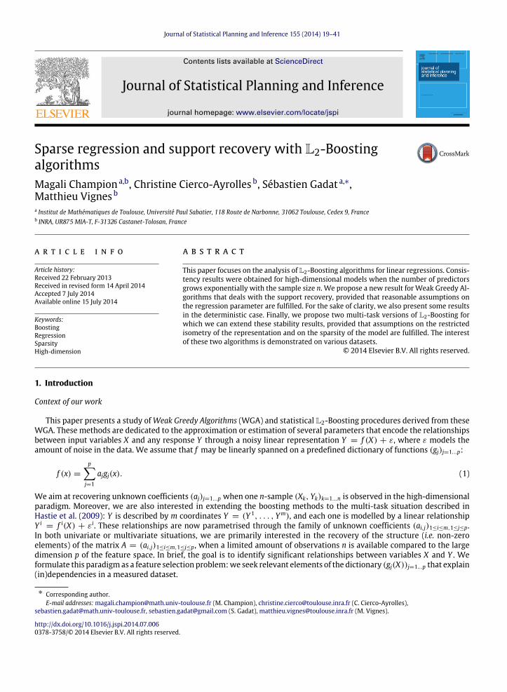
Table 1First dataset: MSE for the Boosting algorithms, with a shrinkage factor γ = 0.2, compared to the BootLasso,RForests and REM; the sample size n is set to 100.

(p,m, S) (250, 1, 5) (250, 1, 10) (1000, 1, 20) (250, 5, 50) (250, 250, 1250)

WGA 0.21 0.23 0.42 ∅ ∅

D-Corr ∅ ∅ ∅ 0.39 0.36L2 norm ∅ ∅ ∅ 0.40 0.38BootLasso 0.30 0.28 0.78 0.31 0.40RForests 0.18 0.25 0.49 0.41 0.20a

REM 0.33 0.18 0.08 0.21 0.19a For 5 simulated replicate datasets only as the running time for RForest was 4 days per network.

Table 2First dataset: Percentage of false positive FP coefficients and false negative FN coefficients for the Boosting algorithms, with a shrinkage factor γ = 0.2,compared to the BootLasso, RForests and REM; the sample size n is set to 100.

(p,m, S) (250, 1, 5) (250, 1, 10) (1000, 1, 20) (250, 5, 50) (250, 250, 1250)FP FN FP FN FP FN FP FN FP FN

FP FN FP FN FP FN FP FN FP FNWGA 0.00 0.00 0.43 0.10 0.62 41.5 ∅ ∅ ∅ ∅

D-Corr ∅ ∅ ∅ ∅ ∅ ∅ 0.84 3.42 0.10 0.65L2 norm ∅ ∅ ∅ ∅ ∅ ∅ 0.85 4.68 0.09 0.73BootLasso 0.00 19.00 0.03 30.70 0.00 89.25 0.10 31.80 0.00 32.03RForests 2.10 0.20 3.67 23.10 1.01 60.25 3.29 32.02 2.47a 2.76a

REM 0.58 0.00 1.49 0.00 5.53 6.65 2.66 0.00 2.35 0.00a For 5 simulated replicate datasets only as the running time for RForest was 4 days per network.

In all our simulations, we always generate n = 100 observations; this situation corresponds to either moderate or veryhigh-dimensional settings, depending on the number of explanatory variables (p) or on the number of response variables(m). Unless otherwise stated, all experiments are replicated 100 times and results are averaged over these replicates.

Prediction performances of tested methods are detailed in Table 1. In the first three simulation settings, when m = 1,the prediction performances of the Boosting algorithms are quite similar to those of the BootLasso and RF ones (see Table 1),but when the number of predictors is set to 1000, BootLasso results are poorer. REM seems to achieve a better predictionthan other approaches, especially in the very high-dimensional settings (p = 1000 whilem = 1). This is still the case whenp = 250 andm = 5 or 250.

Looking at the accuracy results of Table 2 at the same time is instructive: neither BootLasso nor RF succeed at recoveringthe structure of f , with the FN rate much higher than that of the L2-Boosting and REM approaches. In the moderately high-dimensional univariate setting (p,m) = (250, 1), WGA and REM almost always recover the full model with few FP, whileBootLasso and RFmiss one third and one fourth of the correct edges, respectively. Figures in the high-dimensional univariatecase (p,m) = (1000, 1) confirm this trend with a better precision for WGA, whereas REM achieves a better recall. Thisprobably explains the much lower MSE for REM: the model selected in the REM framework is much richer and contains thevast majority of relevant relationships at the price of a low precision (just below 30%). In contrast, the model built by WGAis sparser with fewer FP, but misses some correct relationships. We therefore empirically observe here that MSE is not tooinformative for feature selection, as reported by Hastie et al. (2009), for example. The conclusion we can draw follows thesame tendency in the high-dimensional multivariate settings (p,m) = (250, 5) and (p,m) = (250, 250). Again, REM ismore comprehensive in retrieving actual edges, but it produces much more FP relationships than the multivariate boostingalgorithms we presented.

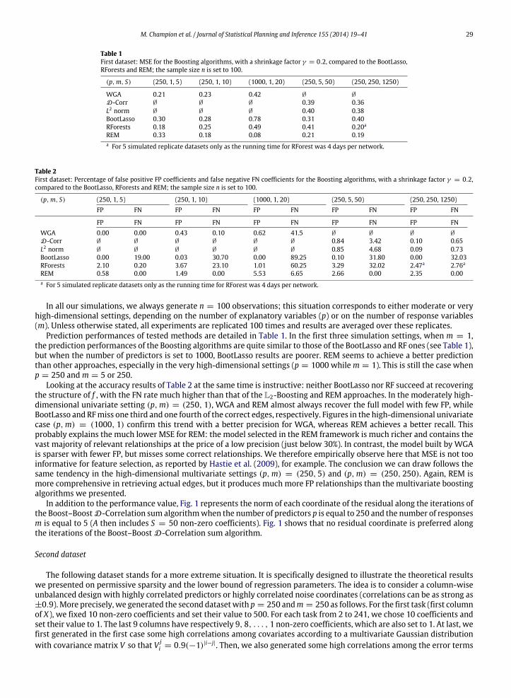
In addition to the performance value, Fig. 1 represents the norm of each coordinate of the residual along the iterations ofthe Boost–BoostD-Correlation sum algorithmwhen the number of predictors p is equal to 250 and the number of responsesm is equal to 5 (A then includes S = 50 non-zero coefficients). Fig. 1 shows that no residual coordinate is preferred alongthe iterations of the Boost–Boost D-Correlation sum algorithm.

Second dataset

The following dataset stands for a more extreme situation. It is specifically designed to illustrate the theoretical resultswe presented on permissive sparsity and the lower bound of regression parameters. The idea is to consider a column-wiseunbalanced design with highly correlated predictors or highly correlated noise coordinates (correlations can be as strong as±0.9).More precisely, we generated the second datasetwith p = 250 andm = 250 as follows. For the first task (first columnof X), we fixed 10 non-zero coefficients and set their value to 500. For each task from 2 to 241, we chose 10 coefficients andset their value to 1. The last 9 columns have respectively 9, 8, . . . , 1 non-zero coefficients, which are also set to 1. At last, wefirst generated in the first case some high correlations among covariates according to a multivariate Gaussian distributionwith covariance matrix V so that V j

i = 0.9(−1)|i−j|. Then, we also generated some high correlations among the error terms


Fig. 1. First dataset (p,m, S) = (250, 5, 50): Norm of each coordinate of residuals along the first 100 iterations of the Boost–Boost D-Correlation sumalgorithm; the sample size n is set to 100.

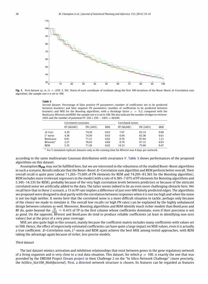
Table 3Second dataset: Percentage of false positive FP parameters (number of coefficients not to be predictedbetween brackets) and false negative FN parameters (number of coefficients to be predicted betweenbrackets) and MSE for the Boosting algorithms, with a shrinkage factor γ = 0.2, compared with theBootLasso, RForests andREM; the sample sizen is set to 100.We also indicate the number of edges to retrieve:2455 and the number of potential FP: 250 ∗ 250 − 2455 = 60,045.

Correlated covariates Correlated noisesFP (60,045) FN (2455) MSE FP (60,045) FN (2455) MSE

D-Corr 4.39 74.20 0.63 7.07 83.14 0.60L2 norm 4.38 74.50 0.63 6.94 83.38 0.61BootLasso 0.81 77.21 0.82 0.76 87.64 1.21RForestsa 2.27 78.63 0.84 0.79 97.15 0.93REM 5.35 71.26 0.62 14.33 75.60 0.47a For 5 simulated replicate datasets only as the running time for RForest was 4 days per network.

according to the same multivariate Gaussian distribution with covariance V . Table 3 shows performances of the proposedalgorithms on this dataset.

AssumptionHSNR may not be fulfilled here, but we are interested in the robustness of the studied Boost–Boost algorithmsin such a scenario. Results indicate that the Boost–BoostD-Correlation sumalgorithm and REMperformbetter overall. Theiroverall recall is quite poor (about 71.26%–75.60% of FN elements for REM and 74.20%–83.36% for the Boosting algorithm).REM includesmore irrelevant regressors in themodel (with a rate of 4.38%–7.07% of FP elements for Boosting algorithms and5.34%–14.33% for REM), probably because of the very high correlation levels between predictors or because of the intricatecorrelated noise we artificially added to the data. The latter seems indeed to be an even more challenging obstacle here. Werecall here that in these 2 scenarii, a 1% in FP rate implies a difference of just over 600 falsely predicted edges. The algorithmsweproposedwere designed to deal partlywith the correlation between responseswhen it is not too high andwhen the noiseis not too high neither. It seems here that the correlated noise is a more difficult situation to tackle, perhaps only becauseof the choice we made to simulate it. The overall low recalls (or high FN rates) can be explained by the highly unbalanceddesign between columns as well. Moreover, Boosting algorithms and REM identify much richer models than BootLasso andRF do, quite beyond the 10

2455 ≈ 0.41% of TP in the first column whose coefficients dominate, even if their precision is notas good. On the opposite, RForest and BootLasso do tend to produce reliable coefficients (at least in identifying non-zerovalues) but at the price of a very poor coverage.

MSE are also quite high in this scenarii, mainly because the coefficient matrix includes many coefficients with values setto 500. Hence, the effect of imprecisely estimated coefficients can have quite a large impact onMSE values, even it is actuallya true coefficient. D-Correlation sum, L2-norm and REM again achieve the best MSE among tested approaches, with REMtaking the advantage again because of richer, less precise models.

Third dataset

The last dataset mimics activation and inhibition relationships that exist between genes in the gene regulatory networkof a living organism and is very close to a real data situation. This dataset, for which p = 100, is exactly the one that wasprovided by the DREAM Project Dream project in their Challenge 2 on the ‘‘In Silico Network Challenge’’ (more precisely,the InSilico_Size100_Multifactorial). First, a directed network structure is chosen. Its features can be regarded as features


Table 4Third dataset: Percentage of false positive FP parameters (number of coefficients not to be predicted betweenbrackets) and false negative FN parameters (number of coefficients to be predicted between brackets) andMSE for the Boosting algorithms, with a shrinkage factor γ = 0.2, compared to the BootLasso, RForests andREM.

FP (9695) FN (205) MSE

D-Corr 21.37 47.75 0.45L2 norm 18.98 50.20 0.50BootLasso 1.40 77.93 0.32RForests 7.68 68.98 0.20REM 7.05 78.53 0.01

Table 5Smallest and largest eigenvalue of the restricted matrix, ratio of these eigenvalues and computation ofρ := maxj∈S ∥D+

S gj∥1 for the three datasets.

λmin λmax λmax/λmin ρ

First dataset(p,m, S) = (250, 1, 5) 75.31 130.43 1.73 0.82





Second datasetCorrelated covariates 3.95 921.39 233.44 5.47

Correlated noises 41.12 181.49 4.41 1.88

Third dataset 19.29 233.83 12.12 1.57

of a biological network, e.g., in terms of degree distribution. Coupled ordinary differential equations (ODEs) then drive thequantitative impact of gene expression on each other, the expression of a gene roughly representing its activity in the system.For example, if gene 1 is linked to gene 2 with a positive effect going from 1 to 2, then increasing the expression of gene 1(as operator do, see Pearl (2009)) will increase the expression of gene 2. However, increasing the expression of gene 2 doesnot have a direct effect on gene 1. Lastly, the system of ODEs is solved numerically to obtain steady states of the expressionof the genes after technical and biological noises are created. We denote as A the n × p expression matrix of p genes for nindividuals. This simulation process is highly non-linear compared to the first two scenarios described above.

The goal was to automatically retrieve network structure encoded in matrix A from data only. Samples were obtained bymultifactorial perturbations of the network using GeneNetWeaver (Schaffter et al., 2011) for simulations. A multifactorialperturbation is the simultaneous effect of numerous minor random perturbations in the network. It therefore measures adeviation from the equilibrium of the system. This could be seen as changes in the network due to very small environmentalchanges or genetic diversity in the population. Additional details and a discussion on the biological plausibility (networkstructure, the use of chemical Langevin differential equations, system and experimental noise) of such datasets can be foundin Marbach et al. (2009).

The results of tested methods on this last dataset are presented in Table 4. In this scenario, our two multivariate (werecall that m = p = 100) L2-Boosting algorithms both suffer from higher MSE. It also exhibits higher FP rates than othercompeting methods: ≈20% vs. 1.4, 7.7 and 7.1% for BootLasso, RF and REM, respectively. Many FP coefficients may implyan increase in MSE, whereas the three other tested methods focus on fewer correct edges.

What can first be considered as a pitfall can be turned into a strength: recall can be close to (for L2 norm) or even higherthan (D-Correlation sum) 50%, whereas other approaches reach 31% at best (RF). In other words, theD-Correlation sum canretrieve more than half of the 205 edges to be predicted, at the price of producing more FP predictions, considered as noisefrom a model prediction perspective in the delivered list. RF is on average only able to grab 84 out of the 205 correct edges,but the prediction list is cleaner in a sense. A specifically designed variant of the RF approach that we tested was deemedthe best performer for this challenge by the DREAM4 organisers (Huynh-Thu et al., 2010). Our algorithm would have beenranked 2nd.

For the sake of completeness, we computed the smallest and the largest eigenvalues of the restricted matrix tDSDS ,that are involved in the key Assumptions HRE− and HRE+ . We also provided the measured value of ρ := maxj∈S ∥D+

S gj∥1of Assumption HS in Table 5 for the three datasets, which quantifies the coherence of the dictionary: favourable situationscorrespond to small values of ρ, ideally lower than 1.


Regarding the first dataset, we obtain a larger value than 0 for λmin and a moderate value of λmax. This implies areasonable value of λmax/λmin. This situation is thus acceptable according to the bound given by Eqs. (33) and (35) (seeAppendix, Lemma B.2). Concerning Assumption HS, for each range of parameters on the first dataset, ρ is not very farfrom 1, which explains the good numerical results. We have to particularly emphasise the first simulation study where(p,m, S) = (250, 1, 5). With a coherence value ρ lower than 1, theWGA reaches to recover the true support of A. λmax/λminand ρ values for the second dataset support our numerical analysis (see Table 3) that shows that this is a very difficultdataset. This situation is clearly less favourable for the sparse estimation provided by our Boosting procedures than for thefirst dataset. This is perhaps less visible for the second simulated setting, where additional noise was correlated. Clearlyin this latter case, hypothesis HMult

dim-3 is violated because the noise coordinates are not i.i.d. anymore. We however have nonumerical indicator to quantify this.

For the last dataset, we can observe that HS yields a moderate value of ρ but that the ratio of the restricted eigenvaluesis quite large (compared to those obtained in the first dataset) and it is difficult to recover the support of the true network.

Taken together, this numerically shows that both HS and HRE− , HRE+ are important to obtain good reconstructionproperties. These assumptions then seem complementary and not redundant. However, the practical use of the proposedalgorithms advocates a certain tolerance of the method towards divergence from the hypotheses that condition ourtheoretical results.

5. Concluding remarks

We studied WGA and established a support recovery result for solving linear regression in high-dimensional settings.We then proposed two statistically funded L2-Boosting algorithms derived thereupon in a multivariate framework. Thealgorithms were developed to sequentially estimate unknown parameters in a high-dimensional regression framework:significant possibly correlated regressor functions from a dictionary need be identified, relative coefficients need beestimated and noise can disturb the observations. Consistency of two variants of the algorithms was proved in Theorem 3.2for the L2 norm variant and in Theorem 3.3 for the D-Correlation sum variant. An important Support Recovery result(Theorem 3.4) under mild assumption on the sparsity of the regression function and on the restricted isometry of the Xmatrix then generalises the univariate result to the multi-task framework. Using the MSE of the model, we derived a simpleyet effective stopping criterion for our algorithms.

We then illustrated the proposed algorithms in a variety of simulated datasets in order to determine the ability ofthe proposed method to compete with state-of-the-art methods when the data is high-dimensional, noisy and the activeelements can be unbalanced. Even if the algorithms we propose are not superior in all settings, we observed, for example,that they are very competitive in situations such as those of the DREAM4 In SilicoMultifactorial Network Challenge.Withoutfine parameter tuning and with a very small computing time, our generic method would have ranked 2nd in this challenge.Moreover, it has the ability to quickly produce a rich prediction list of edges at an acceptable quality level, which mightreveal novel regulatory mechanisms on real biological datasets.

Acknowledgements

Thanks are due to the anonymous reviewer, to the Associate Editor and to our colleagues whose suggestions greatlyimproved this manuscript.

Appendix A. Stability results for Boosting algorithms

A.1. Concentration inequalities

We begin by recalling some technical results. Lemma A.1, given in Bühlmann (2006), provides a uniform law of largenumbers, in order to compare inner products ⟨, ⟩(n) and ⟨, ⟩. It is useful to prove the theorems of Sections 2.2.2 and 2.3, anddoes not rely on boosting arguments.

Lemma A.1. Assume that Hypotheses Hdim are fulfilled on dictionary D , f and ε, with 0 < ξ < 1 as given in Hdim-2, then:(i) sup1≤i,j≤pn |⟨gi, gj⟩(n) − ⟨gi, gj⟩| = ζn,1 = OP(n−ξ/2),(ii) sup1≤i≤pn |⟨gi, ε⟩(n)| = ζn,2 = OP(n−ξ/2),(iii) sup1≤i≤pn |⟨f , gi⟩(n) − ⟨f , gi⟩| = ζn,3 = OP(n−ξ/2).

Denote ζn = maxζn,1, ζn,2, ζn,3, ζn,4 = OP(n−ξ/2). The following lemma (Lemma 2 from Bühlmann (2006)) also holds.

Lemma A.2. UnderHypothesesHdim, a constant 0 < C < +∞ exists, independent of n and k, so that on set Ωn = ω, |ζn(ω)| <1/2:

sup1≤j≤pn

|⟨Rk(f ), gj⟩(n) − ⟨Rk(f ), gj⟩| ≤ C52

k

ζn.


Proof. This lemma is given in Bühlmann (2006), but their notations are confusing since residuals Rk are used to compute ϕk

instead of Y − Gk (see Remark 1 at the end of Section 2.2). It is nevertheless possible to generalise its application field usingLemma A.1. First, assume that k = 0. The desired inequality follows directly from point (iii) of Lemma A.1. We now extendthe proof by an inductive argument.

Denote An(k, j) = ⟨Rk(f ), gj⟩(n)−⟨Rk(f ), gj⟩. Then, on the basis of the recursive relationships of Eqs. (7) and (8), we obtain:

An(k, j) = ⟨Rk−1(f ) − γ ⟨Rk−1(f ), ϕk⟩(n)ϕk − γ ⟨ε, ϕk⟩(n)ϕk, gj⟩(n) − ⟨Rk−1(f ) − γ ⟨Rk−1(f ), ϕk⟩ϕk, gj⟩

= An(k − 1, j) − γ ⟨Rk−1(f ), ϕk⟩(⟨ϕk, gj⟩(n) − ⟨ϕk, gj⟩) =(I)

−γ ⟨ϕk, gj⟩(n)(⟨Rk−1(f ), ϕk⟩(n) − ⟨Rk−1(f ), ϕk⟩) =(II)

−γ ⟨ε, ϕk⟩(n)⟨ϕk, gj⟩(n) =(III)

.

Expanding Eq. (8) yields ∥Rk(f )∥2= ∥Rk−1(f )∥2

− γ (2− γ )⟨Rk−1(f ), ϕk⟩2. From the last equality, we deduce ∥Rk(f )∥2

≤

∥Rk−1(f )∥2≤ · · · ≤ ∥f ∥2 and Lemma A.1(i) shows that

sup1≤j≤pn

|(I)| ≤ ∥Rk−1(f )∥∥ϕk∥ζn ≤ ∥f ∥ζn.

Moreover,

sup1≤j≤pn

|(II)| ≤ sup1≤j≤pn

|⟨ϕk, gj⟩(n)| sup1≤j≤pn

|An(k − 1, j)|

≤ ( sup1≤j≤pn

|⟨ϕk, gj⟩| + ζn) sup1≤j≤pn

|An(k − 1, j)| by (i) of Lemma A.1

≤ (1 + ζn) sup1≤j≤pn

|An(k − 1, j)|.

Finally, using (i) and (ii) from Lemma A.1:

sup1≤j≤pn

|(III)| ≤ sup1≤j≤pn

|⟨ϕk, gj⟩(n)| sup1≤j≤pn

|⟨εik , gj⟩(n)| ≤ (1 + ζn)ζn.

Using our bounds on (I), (II) and (III), and γ < 1, we obtain on Ωn

sup1≤j≤pn

|An(k, j)| ≤ sup1≤j≤pn

|An(k − 1, j)| + ζn∥f ∥ + (1 + ζn) sup1≤j≤pn

|An(k − 1, j)| + (1 + ζn)ζn

≤52

sup1≤j≤pn

|An(k − 1, j)| + ζn

∥f ∥ +

32

.

A simple induction yields:

sup1≤j≤pn

|An(k, j)| ≤

52

k

sup1≤j≤pn

|An(0, j)| ≤ζn

+ζn

∥f ∥ +

32

k−1ℓ=0

52

ℓ

≤

52

k

ζn

1 +

supn∈N

pnj=1

|aj| +32

∞

ℓ=1

52

−ℓ

,

which ends the proof of (i) by setting C = 1 +supn∈N

pnj=1 |aj| +

32

∞

ℓ=1

52

−ℓ.

A.2. Proof of consistency result

We aim then to apply Theorem 2.1 to the semi-population Rk(f ) version of Rk(f ). This will be possible with highprobability when n → +∞. We first observe that Lemma A.2 holds when replacing the theoretical residual Rk(f ) withthe observed residual Y − Gk(f ), thanks to Lemma A.1(ii). Hence, on the set Ωn, by definition of ϕk:

|⟨Y − Gk−1(f ), ϕk⟩(n)| = sup1≤j≤pn

|⟨Y − Gk−1(f ), gj⟩(n)|

= sup1≤j≤pn

|⟨Rk−1(f ), gj⟩| − C

52

k−1

ζn

. (15)


Applying Lemma A.2 again on the set Ωn, we have:

|⟨Rk−1(f ), ϕk⟩| ≥ |⟨Y − Gk−1(f ), ϕk⟩(n)| − C52

k−1

ζn

≥ sup1≤j≤pn

|⟨Rk−1(f ), gj⟩| − 2C52

k−1

ζn. (16)

Let Ωn = ω, ∀k ≤ kn, sup1≤j≤pn |⟨Rk−1(f ), gj⟩| > 4C 52

k−1ζn. We deduce the following equality from Eq. (16):

|⟨Rk−1(f ), ϕk⟩| ≥12

sup1≤j≤pn

|⟨Rk−1(f ), gj⟩|. (17)

Consequently, on the set Ωn ∩ Ωn, we can apply Theorem 2.1 to the family (Rk(f i))k, since it satisfies a WGA with constantsν = 1/2.

∥Rk(f )∥ ≤ CB

1 +

14γ (2 − γ )k

−2−γ

2(6−γ )

. (18)

Now consider the set ΩCn = ω, ∃ k ≤ kn sup1≤j≤pn |⟨Rk−1(f ), gj⟩| ≤ 4C

52

k−1ζn. Note that:

∥Rk(f )∥2= ⟨Rk(f ), f − γ

k−1j=0

⟨Rj(f ), ϕj⟩ϕj⟩

≤

pnj=1

|aj| + γ

k−1j=0

|⟨Rj(f ), ϕj⟩|

sup

1≤j≤pn|⟨Rk(f ), gj⟩|.

Then, since ∥Rk(f )∥ is non-increasing and by definition of ΩCn , we deduce that on ΩC

n ,

∥Rk(f )∥2≤ 4C

52

k

ζn

pnj=1

|aj| + γ k∥f ∥

. (19)

Hence, on (Ωn ∩ Ωn) ∪ ΩCn , using Eqs. (18) and (19),

∥Rk(f )∥2≤ C2

B

1 +

14γ (2 − γ )k

−2−γ6−γ

+ 4C52

k

ζn

pnj=1

|aj| + γ k∥f ∥

. (20)

To conclude, note thatP(Ωn ∩ Ωn) ∪ ΩC

n

≥ P(Ωn) −→

n→+∞1. Inequality (20) holds almost surely for allω and for a sequence

kn < (ξ/4 log(3)) log(n), which grows sufficiently slowly:

∥Rkn(f )∥ = oP(1). (21)

To end the proof, let k ≥ 1 and consider Ak = ∥Rk(f ) − Rk(f )∥. By definition:

Ak =

Rk−1(f ) − γ ⟨Rk−1(f ), ϕk⟩(n)ϕk − γ ⟨ε, ϕk⟩(n)ϕk −

Rk−1(f ) − γ ⟨Rk−1(f ), ϕk⟩ϕk

≤ Ak−1 + γ |⟨Y − Gk−1(f ), ϕk⟩(n) − ⟨Rk−1(f ), ϕk⟩|. (22)

Under Hypothesis Hdim, we deduce the following inequality on Ωn from Eq. (22):

Ak ≤ Ak−1 + γ

C52

k−1

+ 1

ζn. (23)

Using A0 = 0, we deduce recursively from Eq. (23) that, on Ωn, since k := kn grows sufficiently slowly:

AknP

−−−−→n→+∞

0. (24)

Finally, observe that ∥Rkn(f )∥ ≤ ∥Rkn(f )∥ + Akn . The conclusion holds using Eqs. (21) and (24).


A.3. Proof of support recovery

We now detail the proof of Theorem 2.3, which represents the exact recovery of the support with high probability. Itshould be recalled that we denote as S (respectively, S) the sparsity (respectively, the support) of f . We suppose that thecurrent residuals could be decomposed on D as Rk(f ) =

pnj=1 θ k

j gj, where (θ kj )j is Sk-sparse, with support Sk.

Proof of (i). The aim of the first part of the proof is to show that along the iterations of Boosting, we only select elementsof the support of f using Eq. (5). Since S0 = S, we only have to show that (Sk)k≥0 is non-increasing, which implies thatsuccessive residual supports satisfy Sk ⊂ Sk−1. At the initial step k = 0, S0 = S and S0 = S. The proof works now byinduction, and we assume that Sk−1 ⊂ S. Using the same outline as that of the proof of Lemma A.2, we have:

∀gj ∈ D, |⟨Y − Gk−1(f ), gj⟩(n) − ⟨Rk−1(f ), gj⟩| ≤ Cζn

52

k−1

. (25)

On the one hand, we deduce from Eq. (25) below that:

∀j ∈ Sk−1, |⟨Y − Gk−1(f ), gj⟩(n)| ≥ |⟨Rk−1(f ), gj⟩| − Cζn

52

k−1

. (26)

On the other hand, for j ∈ Sk−1, we also have:

|⟨Y − Gk−1(f ), gj⟩(n)| ≤ |⟨Rk−1(f ), gj⟩| + Cζn

52

k−1

. (27)

Now denote Mk := maxj∈Sk−1 |⟨Rk−1(f ), gj⟩| and MCk := maxj∈Sk−1 |⟨Rk−1(f ), gj⟩|. We recall that element j is selected at

step k following Eq. (5). Hence, we deduce from Eqs. (26) and (27) that j ∈ Sk is in Sk−1 if the following inequality issatisfied:

Mk > MCk + 2Cζn

52

k−1

. (28)

The next step of the proof consists in comparing the two quantities Mk and MCk . Note that M and MC can be rewritten as

∥tDSk−1 Rk−1(f )∥∞ and ∥

tDSCk−1

Rk−1(f )∥∞. Following the arguments of Tropp (2004), we have:

Mk

MCk

=

∥tDSC

k−1

tD+

Sk−1tDSk−1 Rk−1(f )∥∞

∥tDSk−1 Rk−1(f )∥∞

≤ ∥tDSC

k−1

tD+

Sk−1∥∞,∞,

where ∥.∥q,q is the subordinate norm of the space (Rq, ∥.∥q). In particular, the norm ∥.∥∞,∞ equals the maximum absoluterow of its arguments, and we also have:

Mk

MCk

≤ ∥D+

Sk−1DSC

k−1∥1,1 = max

j∈Sk−1∥D+

Sk−1gj∥1.

Using Assumption HS and the recursive assumption Sk−1 ⊂ S, we obtain thatMk > MCk .

The end of the proof of (i) follows with Eq. (28) for k := kn given by Theorem 2.2, which implies that ζn(5/2)k → 0.

Proof of (ii). The second part of the proof consists in checking that, along the iterations of the Boosting algorithm, everycorrect element of the dictionary is chosen at least once.

Assume that one element j0 of S is never selected. Then, if we denote θ k= (θ k

j )1≤j≤pn as the decomposition of Rk−1(f )on D , we obtain:

∥θ k∥2

=

j

(θ kj )

2≥ (θ k

j0)2

= a2j0 , (29)

where aj0 is the true coefficient of f associated with the element gj0 .Moreover, note that

∥Rk−1(f )∥2= ∥Dθ k

∥2

≥ λmin∥θk∥2, (30)

with λmin := infβ,Supp(β)⊂S ∥Dβ∥2/∥β∥

2 > 0 by Assumption HRE− .


Eq. (30) deserves special attention since (∥Rk−1(f )∥)k decreaseswith k. More precisely, Eqs. (20) and (23) of Appendix A.2provide the following bound for ∥Rk−1(f )∥:

∥Rk−1(f )∥2≤ (C log(n))−α ,

where α :=2−γ

6−γ.

The sought contradiction is obtained using Assumption HSNR in Eq. (29) as soon as

λmin log(n)−2κ≥ (C log(n))−α ,

i.e., when κ < κ∗:= (2 − γ )/2(6 − γ ). This ends the proof of the support consistency.

Appendix B. Proof for multi-task L2-Boosting algorithms

B.1. Proof of Theorem 3.1

We break down the proof of Theorem 3.1 into several steps here. It should be recalled that D = (gj), 1 ≤ j ≤ p is adictionary that spans H . We set any f = (f 1, . . . , f m) ∈ Hm so that f i ∈ A(D, B).

The first key remark is that if we denote si(k) as the number of steps in which i is invoked until step k, for all i ∈ [[1,m]],we deduce from Theorem 2.1 that:

∀k ≥ 1, ∥Rk−1(f i)∥ ≤ CB(1 + ν2γ (2 − γ )si(k − 1))−ν(2−γ )

2(2+ν(2−γ )) . (31)

The second key point of the proof consists in comparing Rk(f i) and Rk(f ik), where ik is chosen using Eq. (10) or (11). Forthe Boost–Boost Residual L2 norm algorithm, this step is not pivotal since, using Eq. (10):

sup1≤i≤m

∥Rk(f i)∥ ≤ µ−1∥Rk(f ik)∥. (32)

However, for the Boost–Boost D-Correlation sum algorithm, we can prove the following lemma:

Lemma B.1. Suppose that Assumptions HRE− and HRE+ hold. Then, for any k:

sup1≤i≤m

∥Rk−1(f i)∥2≤ µ−1

∥Rk−1(f ik)∥2

λmax

λmin

3

,

where λmin and λmax (given by Assumptions HRE− and HRE+ ) are the smallest and the largest eigenvalues tDSDS .

Proof. Assume that each residual Rk(f i) is expanded on D at step k as: Rk(f i) =p

j=1 θ ki,jgj, where (θ k

i,j)1≤j≤p is S ik-sparse,with support Si

k. Note that, along the iterations of the Boost–Boost algorithm, an incorrect element of the dictionary cannotbe selected using Eq. (12) (see Theorem 3.4 for some supplementary details). We observe then that Assumptions HRE− andHRE+ imply that at each step, each approximation is at most S-sparse. We present an elementary lemma that will be veryuseful until the end of the proof.

Lemma B.2. Let D = (g1, . . . , gp) be a dictionary on H. Denote D as the matrix whose columns are the elements of D , and forany S ⊂ [[1, p]], DS the matrix restricted to the elements of D that are in S. Then, if we denote λmin and λmax as the smallest andthe largest eigenvalues of the restricted matrix tDSDS , the two propositions hold.

(i) For any S-sparse family (aj)1≤j≤p, we have:

λmin

p

j=1

|aj|2

≤

pj=1

ajgj

2

≤ λmax

p

j=1

|aj|2

.

(ii) For any function f spanned on D as f =p

j=1 ajgj, where (aj)j is S-sparse, we have:

λ2min

p

j=1

|aj|21/2

≤

p

j=1

|⟨f , gj⟩|21/2

≤ λ2max

p

j=1

|aj|21/2

.

Now, let i = ik. By Lemma B.2 (right hand side – r.h.s. – of (ii) and left hand side – l.h.s. – of (i)) combinedwith AssumptionHRE− , we have:

pj=1

|⟨Rk−1(f ik), gj⟩|2 ≤ ∥Rk−1(f ik)∥2 λ2max

λmin. (33)


Moreover Lemma B.2 again (l.h.s. of (ii) and r.h.s. of (i)) and Assumption HRE+ show that:

∀1 ≤ i ≤ m,

pj=1

|⟨Rk−1(f i), gj⟩|2 ≥ ∥Rk−1(f i)∥2 λ2min

λmax. (34)

By definition of ik (see Eq. (11) in the Boost–Boost algorithm), we deduce that:

∀i ∈ [[1,m]],

pj=1

|⟨Rk−1(f ik), gj⟩|2 ≥ µ

pj=1

|⟨Rk−1(f i), gj⟩|2

≥ µ∥Rk−1(f i)∥2 λ2min

λmax. (35)

The conclusion follows by using Eqs. (33) and (35).

To conclude, we consider the Euclidean division of k by m: k = mK + d, where the remainder d is not greater than thedivisor m. A coordinate i∗ ∈ 1 . . .m, that is selected at least K times by Eq. (10) or (11) exists, hence si∗(k) ≥ K . We alsodenote k∗ as the last step that selects i∗ before step k. Since

∥Rk(f i)∥

k is a non-increasing sequence along the iterations of

the algorithm, Eq. (31) leads to:

∥Rk−1(f i∗

)∥ ≤ ∥Rk∗−1(f i∗

)∥ ≤ CB(1 + ν2γ (2 − γ )(K − 1))−ν(2−γ )

2(2+ν(2−γ )) . (36)

The conclusion holds noting that km − 1 ≤ K ≤

km and ν < 1, and using our bounds (32) for the Boost–Boost Residual L2

norm algorithm, or Lemma B.1 for the Boost–Boost D-Correlation sum algorithm.

B.2. Proof of Theorem 3.4

We begin this section by clarifying the proof of Theorem 3.4 since this result is needed to prove all other multi-taskresults. The proof proceeds in the same way as in Appendix A.3. Our focus is on the choice of the regressor to add in themodel, regardless of the column chosen to be regressed in the previous step. Therefore, in order to simplify notations, indexi may be omitted and we can do exactly the same computations.

B.3. Proof of Theorems 3.2 and 3.3

The proof of consistency results in the multi-task case is the same as in Appendix A.2. Hence, we consider a semi-population version of the two Boost–Boost algorithms: let (Rk(f ))k be the phantom residuals, that are now living in Hm,initialised by R0(f ) = f , and satisfy at step k:

Rk(f i) = Rk−1(f i) if i = ik,

Rk(f ik) = Rk−1(f ik) − γ ⟨Rk−1(f ik), ϕk⟩ϕk, (37)

where (ik, ϕk) is chosen according to Algorithm 4.As previously explained, we aim at applying Theorem 3.1 to the phantom residuals. This will be possible if we can show

an analogue of Eqs. (10) (for the Residual L2 norm) or (11) (for the D-Correlation sum) and (12). Note that on the basis ofTheorem 3.4, the sparsity of both residuals Rk(f ) and Rk(f ) does not exceed S with high probability if we choose γ smallenough in Eq. (13).

We begin the proof by recalling Lemma A.1. In the multi-task case, this lemma can be easily extended as follows:

Lemma B.3. Assume that Hypotheses HMultdim are fulfilled on dictionary D , f and ε, with 0 < ξ < 1 as given in HMult

dim-2, then:(i) sup1≤i,j≤pn |⟨gi, gj⟩(n) − ⟨gi, gj⟩| = ζn,1 = OP(n−ξ/2),(ii) sup1≤i≤pn,1≤j≤mn |⟨gi, εj

⟩(n)| = ζn,2 = OP(n−ξ/2),(iii) sup1≤i≤mn,1≤j≤pn |⟨f i, gj⟩(n) − ⟨f i, gj⟩| = ζn,3 = OP(n−ξ/2),(iv) sup1≤i≤mn |∥εi

∥2(n) − E(|εi |2)| = ζn,4 = OP(n−ξ/2).

The first three points of Lemma B.3 are the same as (i), (ii) and (iii) of Lemma A.1. The fourth point is something new.However, since its proof does not call for typical boosting arguments, we do not state it here.

Denoting ζn = maxζn,1, ζn,2, ζn,3, ζn,4 = OP(n−ξ/2), we can show that Lemma A.2 is still true for the ikth coordinate off . Moreover, let i = ik. Since Rk(f i) = Rk′(f i) for all k′

≤ k so that ik is not selected between step k′ and k (see Eq. (13)), wecan easily extend Lemma A.2 to each coordinate of f :

sup1≤i≤mn

sup1≤j≤pn

|⟨Rk(f i), gj⟩(n) − ⟨Rk(f i), gj⟩| ≤ C52

k

ζn. (38)


Using this extension of Lemma A.1, the same calculations detailed in Appendix A.2 can be done. Hence, considering theikth coordinate of f chosen by Eq. (10) or (11), on the set Ωn, inequality (17) also holds:

|⟨R(f ik), ϕk⟩| ≥12

sup1≤j≤pn

|⟨Rk−1(f ik), gj⟩|.

Now consider the Boost–Boost Residual L2 norm algorithm. To obtain an analogue of (10), we need the following lemma,which compares the norms of both residuals:

Lemma B.4. Under Hypotheses HMultdim , a constant 0 < C < +∞ exists, independent of n and k, so that on the set Ωn =

ω, |ζn(ω)| < 1/2:

sup1≤i≤mn

|∥Rk−1(f i)∥2(n) − ∥Rk−1(f i)∥2

| ≤ C

252

k−1

+ S

Sζn.

Proof. Consider the two residual sequences (Rk(f ))k and (Rk(f ))k, expanded on D as: Rk−1(f i) =

j θki,jgj, and Rk−1(f i) =

j θki,jgj. Hence,

|∥Rk−1(f i)∥2(n) − ∥Rk−1(f i)∥2

| ≤

pnj=1

θ ki,j

⟨Rk−1(f i), gj⟩(n) − ⟨Rk−1(f i), gj⟩

(I)

+

pnj=1

θ ki,j

⟨Rk−1(f i), gj⟩(n) − ⟨Rk−1(f i), gj⟩

(II)

+

pnj=1

θ ki,j⟨Rk−1(f i), gj⟩ −

Sj=1

θ ki,j⟨Rk−1(f i), gj⟩(n)

(III)

.

Using Eq. (38), we can provide two upper bounds for (I) and (II):

(I) ≤ C52

k−1 pnj=1

|θ ki,j|ζn and (II) ≤ C

52

k−1 pnj=1

|θ ki,j|ζn.

DenotingM := max1≤j≤S|θki,j|, |θ

ki,j|, the following inequality holds for (I) and (II):

(I) ∨ (II) ≤ CMS52

k−1

ζn.

To conclude, using Lemma B.3, we have:

(III) ≤

pnj=1

|aki,j|pnj′=1

|aki,j||⟨gj, gj′⟩ − ⟨gj, gj′⟩(n)| ≤ S2M2ζn

and the conclusion follows using our last bounds.

Since Lemma B.4 is not directly applicable to the observed residual Y − Gk(f ), the same calculation cannot be performedto obtain an analogue of Eq. (10). However, we can compare the norm of the theoretical and observed residuals:

sup1≤i≤mn

∥Y i− Gk−1(f i)∥2

(n) = ∥Rk−1(f i) + εi∥2(n)

= ∥Rk−1(f i)∥2(n) + ∥εi

∥2(n) + 2⟨Rk−1(f i), εi

⟩(n).

Note that, using Lemma B.3, we obtain: |⟨Rk(f i), εi⟩(n)| ≤ MSζn, where M is defined in the proof of Lemma B.4. Hence, we

have for all i:

∥Rk−1(f i)∥2(n) + ∥εi

∥2(n) − 2MSζn ≤ ∥Y i

− Gk−1(f i)∥2(n) ≤ ∥Rk−1(f i)∥2

(n) + ∥εi∥2(n) + 2MSζn. (39)


It should be recalled that E(|εi|2) does not depend on i from Assumption HMult

dim-3, and is denoted by σ 2. An application ofLemma B.3(iv) to Eq. (39) then yields:

∥Rk−1(f i)∥2(n) + σ 2

− (1 + 2MS)ζn ≤ ∥Y i− Gk−1(f i)∥2

(n) ≤ ∥Rk−1(f i)∥2(n) + σ 2

+ (1 + 2MS)ζn. (40)

Hence, on Ωn, by definition of ik, Eq. (40) and Lemma B.4, we can write:

∥Y ik − Gk−1(f ik)∥2(n) ≥ sup

1≤i≤mn

∥Y i− Gk−1(f i)∥2

(n)

≥ sup1≤i≤mn

∥Rk−1(f i)∥2

(n) + σ 2

− (1 + 2MS)ζn

≥ sup1≤i≤mn

∥Rk−1(f i)∥2

+ σ 2

− C

252

k−1

+ S

Sζn − (1 + 2MS)ζn. (41)

Using the same calculus on the set Ωn once again:

∥Rk−1(f ik)∥2≥ ∥Rk−1(f ik)∥2

(n) − C

252

k−1

+ S

Sζn

≥ ∥Y ik − Gk−1(f ik)∥2(n) − σ 2

− (1 + 2MS)ζn − C

252

k−1

+ S

Sζn

≥ sup1≤i≤mn

∥Rk−1(f i)∥2

+ σ 2

− σ 2− 2(1 + 2MS)ζn − 2C

252

k−1

+ S

Sζn, by Eq. (41). (42)

We then obtain from Eq. (42) that:

∥Rk−1(f ik)∥2≥ sup

1≤i≤mn

∥Rk−1(f i)∥2− 2(1 + 2MS)ζn − 2C

252

k−1

+ S

Sζn. (43)

Let Ω1n = ω, ∀k ≤ kn sup1≤i≤mn ∥Rk−1(f i)∥2 > 4(1 + 2MS + C(2( 5

2 )k−1

+ S)S)ζn. We deduce from Eq. (43) thefollowing inequality on set Ωn ∩ Ω1

n :

∥Rk−1(f ik)∥2≥

12

sup1≤i≤mn

∥Rk−1(f i)∥2.

Finally, consider the Boost–Boost D-Correlation sum algorithm. To obtain an analogue of Eq. (11), the following lemmais needed:

Lemma B.5. Under Hypotheses HMultdim , a constant 0 < C < +∞ exists, independent of n and k so that, on the set Ωn =

ω, |ζn(ω)| < 1/2:

sup1≤i≤m

sup1≤j≤pn

|⟨Rk(f i), gj⟩2(n) − ⟨Rk(f i), gj⟩2| ≤ C52

2k

ζn.

Proof. Let k ≥ 1, i ∈ [[1,mn]]. We have the following equality:

|⟨Rk(f i), gj⟩2(n) − ⟨Rk(f i), gj⟩2| = |⟨Rk(f i), gj⟩(n) − ⟨Rk(f i), gj⟩||⟨Rk(f i), gj⟩(n) + ⟨Rk(f i), gj⟩|, (44)

where |⟨Rk(f i), gj⟩(n) − ⟨Rk(f i), gj⟩| ≤ C 52

kζn by Eq. (38).

Moreover, using the recursive equation for (Rk(f ik))k, we can obtain the following bounds:

|⟨Rk(f ik), gj⟩(n)| ≤ |⟨Rk−1(f ik), gj⟩(n)| + γ |⟨Rk−1(f ik), ϕk⟩(n)⟨ϕk, gj⟩(n)| + γ |⟨εik , ϕk⟩(n)⟨gj, ϕk⟩(n)|

≤ sup1≤j≤pn

|⟨Rk−1(f ik), gj⟩(n)|(1 + γ |⟨ϕk, gj⟩(n)|) + γ ζn(1 + ζn)

≤ M ikk−1(1 + γ (1 + ζn)) + γ ζn(1 + ζn),

whereM ik := sup1≤j≤pn |⟨Rk(f i), gj⟩(n)|. Note that for i = ik, M i

k = M ik−1.

On Ωn, we therefore have, as a suitable constant, C > 0:

M ik ≤ M i

k−1

1 +

32γ

+ C · · · ≤

1 +

32γ

ksupn∈N

pnj=1

|ai,j| +32

+ C . (45)


Using Eq. (8), ∥Rk(f i)∥ is non-increasing and thus ∥Rk(f i)∥ ≤ ∥f i∥. The Cauchy–Schwarz inequality allows us to write that:

|⟨Rk(f i), gj⟩| ≤ ∥Rk(f i)∥ ≤ ∥f i∥. (46)

The conclusion therefore holds using Eqs. (45) and (46) in Eq. (44) for a large enough constant C .

Observe that Lemma B.5 remains true if we change the observed residual by the theoretical residual. Therefore, on theset Ωn,

pnj=1

|⟨Y ik − Gk−1(f ik), gj⟩(n)|2 ≥ sup1≤i≤mn

pnj=1

|⟨Y i− Gk−1(f i), gj⟩(n)|2

≥ sup1≤i≤mn

pnj=1

|⟨Rk−1(f i), gj⟩(n)|2 − C

52

2(k−1)

ζn

≥ sup1≤i≤mn

pnj=1

|⟨Rk−1(f i), gj⟩(n)|2 − Cpn

52

2(k−1)

ζn. (47)

Using Lemma B.5 again on Ωn:pnj=1

|⟨Rk−1(f ik), gj⟩|2 ≥

pnj=1

|⟨Y ik − Gk−1(f ik), gj⟩(n)|2 − Cpn

52

2(k−1)

ζn

≥ sup1≤i≤mn

pnj=1

|⟨Rk−1(f i), gj⟩|2 − 2Cpn

52

2(k−1)

ζn by Eq. (47). (48)

Let Ω2n = ω, ∀k ≤ kn sup1≤i≤mn

pnj=1 |⟨Rk−1(f i), gj⟩|2 > 4Cpn

52

2(k−1)ζn. On the basis of Eq. (48), we can deduce

the following inequality on Ωn ∩ Ω2n :

pnj=1

|⟨Rk−1(f ik), gj⟩|2 ≥12

sup1≤i≤mn

pnj=1

|⟨Rk−1(f i), gj⟩|2.

Consequently, on Ωn ∩ Ωn ∩ Ω1n and Ωn ∩ Ωn ∩ Ω2

n , we can apply Theorem 3.1 to family (Rk(f i))k, since it satisfies adeterministic Boost–Boost algorithm with constants µ = 1/2, ν = 1/2, and has a bounded sparsity S.

Let us now consider the setΩ2

n

C. Using Eq. (34), we obtain

∥Rk(f i)∥2≤

λmax

λ2min

pnj=1

|⟨Rk(f i), gj⟩|2 ≤ 4λmax

λ2min

Cpn

52

2k

ζn.

On the setΩ1

n

C, we also have:

∥Rk(f i)∥2≤ 4

1 + 2MS + C

252

k

+ S

S

ζn.

The end of the proof follows as in Appendix A.2 by noting that P(Ωn ∩ Ωn) ∪ ΩC

n ∪ ΩCn

≥ P(Ωn) −→

n→+∞1. Note that

the conclusion holds for a sequence kn that grows sufficiently slowly: for the Boost–Boost Residual L2 norm algorithm, kn isallowed to grow as (ξ/4 log(3)) log(n), whereas kn can only grow as (ξ/8 log(3)) log(n) for the Boost–Boost D-Correlationsum algorithm.

References

Ambroise, C., McLachlan, G.J., 2002. Selection bias in gene extraction on the basis of mi- croarray gene-expression data. Proc. Natl. Acad. Sci. USA 99,6562–6566.

Anjum, S., Doucet, A., Holmes, C.C., 2009. A boosting approach to structure learning of graphs with and without prior knowledge. Bioinformatics 25 (22),2929–2936.

Bach, F., 2008. Bolasso: model consistent lasso estimation through the bootstrap. In: Proceedings of the Twenty-fifth International Conference onMachineLearning. ACM., Helsinki, Finland, pp. 33–40.

Bühlmann, P., 2006. Boosting for high-dimensional linear models. Ann. Statist. 34 (2), 559–583.Bühlmann, P., Yu, B., 2003. Boosting with the L2-loss: regression and classification. J. Amer. Statist. Assoc. 98 (462), 324–339.Bühlmann, P., Yu, B., 2010. Boosting. In: Wiley Interdisciplinary Reviews: Computational Statistics, vol. 2. pp. 69–74.Blanchard, J.D., Cartis, C., Tanner, J., 2011. Compressed sensing: how sharp is the restricted isometry property?. SIAM Rev. 53 (1), 105–125.

http://refhub.elsevier.com/S0378-3758(14)00120-7/sbref1








Breiman, L., 2001. Random forests. Mach. Learn. 45 (1), 5–32.Cai, T., Jiang, T., 2011. Limiting laws of coherence of random matrices with applications to testing covariance structure and construction of compressed

sensing matrices. Ann. Statist. 39 (3), 1496–1525.Cai, T., Wang, L., 2011. Orthogonal matching pursuit for sparse signal recovery with noise. IEEE Trans. Inform. Theory 57 (7), 4680–4688.Candes, E., Tao, T., 2005. Decoding by linear programming. IEEE Trans. Inform. Theory 51 (12), 4203–4215.Candes, E., Tao, T., 2007. The dantzig selector: Statistical estimation when p is much larger than n. Ann. Statist. 35 (6), 2313–2351.Dream project. Organizers: Columbia university and IBM. Available: http://wiki.c2b2.columbia.edu/dream/index.php/The_DREAM_Project.Eldar, Y., Rauhut, H., 2011. Average case analysis of multichannel sparse recovery using convex relaxation. IEEE Trans. Inform. Theory 56, 505–519.Friedman, J., Hastie, T., Tibshirani, R., 2000. Additive logistic regression. A statistical view of boosting (with discussion). Ann. Statist. 28 (2), 337–407.Gadat, S., 2008. Jump diffusion over feature space for object recognition. SIAM J. Control Optim. 47 (2), 904–935.Gribonval, R., Nielsen, M., 2006. Beyond sparsity: recovering structured representations by L1 minimization and greedy algorithms. Adv. Comput. Math.

28 (1), 23–41.Guyon, I., Weston, J., Barnhill, S., Vapnik, V., 2002. Ene selection for cancer classification using support vector machines. Mach. Learn. 46, 389–422.Hastie, T., Tibshirani, R., Friedman, J., 2009. The Elements of Statistical Learning. Springer.Hocking, R.R., 1983. Developments in linear regression methodology: 1959–1982. Technometrics 25 (6), 219–249.Huynh-Thu, V.A., Irrthum, A., Wehenkel, L., Geurts, P., 2010. Inferring regulatory networks from expression data using tree-based methods. PLoS ONE 5

(9), e12776.Lounici, Karim, Pontil, Massimiliano, van de Geer, Sara, Tsybakov, Alexandre B., 2011. Oracle inequalities and optimal inference under group sparsity. Ann.

Statist. 39 (4), 2164–2204.Lutz, R.W., Bühlmann, P., 2006. Boosting for high multivariate responses in high dimensional linear regression. Statist. Sinica 16 (2), 471–494.Marbach, D., Schaffter, T., Mattiussi, C., Floreano, D., 2009. Generating realistic in silico gene networks for performance assesment of reverse engineering

methods. J. Comput. Biol. 16 (2), 229–239.Meinshausen, N., Rocha, G., Yu, B., 2007. Discussion: A tale of three cousins: Lasso, L2 Boosting and Dantzig. Ann. Statist. 35 (6), 2373–2384.Oates, C.J., Mukherjee, S., 2012. Network inference and biological dynamics. Ann. Appl. Stat. 6 (3), 1209–1235.Obozinski, G., Wainwright, M.J., Jordan, M.I., 2011. Support union recovery in high-dimensional multivariate regression. Annals of Statistics 39, 1–17.Pearl, J., 2009. Causality: Models, Reasoning and Inference, 2nd ed. Cambridge University Press.Peng, J., Zhu, J., Bergamaschi, A., Han,W., Noh, D.-Y., Pollack, J.R., Wang, P., 2010. Regularizedmultivariate regression for identifyingmaster predictors with

application to integrative genomics study of breast cancer. Ann. Appl. Stat. 4 (1), 53–77.Ridgeway, G., 1999. Generalization of boosting algorithms and applications of Bayesian inference for massive datasets (Ph.D. thesis). University of

Washington.Schaffter, T., Marbach, D., Floreano, D., 2011. Genenetweaver: In silico benchmark generation and performance profiling of network inference methods.

Bioinformatics 27 (16), 2263–2270.Schapire, R.E., 1990. The strength of weak learnability. Mach. Learn. 5 (2), 197–227.Schapire, R.E., 1999. Theoretical views of boosting. In: Computational learning theory (Nordkirchen, 1999). In: Lecture Notes in Comput. Sci., vol. 1572.

Springer, Berlin, pp. 1–10.Schapire, R.E., Freund, Y., 1996. Experiments with a new boosting algorithm. In: Proceedings of the Thirteenth International Conference on Machine

Learning. Morgan Kaufman, San Francisco, pp. 148–156.Similä, T., Tikka, J., 2007. Input selection and shrinkage in multiresponse linear regression. Comput. Statist. Data Anal. 52 (1), 406–422.Solnon, M., Arlot, S., Bach, F., Multi-task regression using minimal penalties. Preprint, pages 1–33, 2011.Temlyakov, V.N., 2000. Weak greedy algorithms. Adv. Comput. Math. 12 (2, 3), 213–227.Temlyakov, V.N., Zheltov, P., 2011. On performance of greedy algorithms. J. Approx. Theory 163 (9), 1134–1145.Tibshirani, R., 1996. Regression shrinkage and selection via the lasso. J. R. Stat. Soc. Ser. B Stat. Methodol. 58 (1), 267–288.Tropp, J.A., 2004. Greed is good: algorithmic results for sparse approximation. IEEE Trans. Inform. Theory 50 (10), 2231–2242.Vershynin, R., 2012. Introduction to the non-asymptotic analysis of randommatrices. In: Compressed Sensing. Cambridge University Press.Verzelen, N., 2012. Minimax risks for sparse regressions: Ultra-high dimensional phenomenons. Electron. J. Stat. 6, 38–90.Vignes, M., Vandel, J., Allouche, D., Ramadan-Alban, N., Cierco-Ayrolles, C., Schiex, T., Mangin, B., de Givry, S., 2011. Gene regulatory network reconstruction

using Bayesian networks, the Dantzig selector, the lasso and their meta-analysis. PLoS ONE 6 (12).Wainwright, M., 2009. Information-theoretic limits on sparsity recovery in the high-dimensional and noisy setting. IEEE Trans. Inform. Theory 55,

5728–5741.Yuan, M., Lin, Y., 2007. Model selection and estimation in regression with grouped variables. J. R. Stat. Soc.: Ser. B Stat. Methodol. 68 (1), 49–67.Zhang, T., 2009. On the consistency of feature selection using greedy least squares regression. J. Mach. Learn. Res. 10, 555–568.Zhao, P., Yu, B., 2006. On model selection consistency of Lasso. J. Mach. Learn. Res. 7, 2541–2567.Zou, H., Hastie, T., 2005. Regularization and variable selection via the elastic net. J. Royal Statistical Soc., Ser. B 67, 301–320.






http://wiki.c2b2.columbia.edu/dream/index.php/The_DREAM_Project



































sparse regression and support recovery with l2-boosting algorithms

Documents