SPARC Temperature Trends Assessment group

also Shigeo Yoden, Carl Mears, John Nash

NathanGillett

JimMiller Philippe

Keckhut

DaveThompson

KeithShine

me

UlrikeLangematz

DianSeidel

John Austin

Why Dave isn’t here:

Issues regarding SSU data

1. Construction of data set (Nash up to 1998, NOAA to 2005) - why are climatologies different for x-channels? - why different seasonal cycles? (especially for 47x)

2. How are tidal effects treated? What are the associated uncertainties? What are the other important corrections used in constructing the SSU time series?

3. Evidence for SSU uncertainties, especially after NOAA-14

a) SSU15x comparisons with sondes and MSU4b) comparison of channels with similar weighting functions

(25 and 26x, 27 and 36x)c) unphysical nature of trends after ~1995

4. Where are ‘we’ with respect to original SSU data? (‘we’ = research community)

5. Comments on using SSU in future reanalyses?

-> recommendations from SPARC (to WOAP)?

WOAP = WCRP Observations and Assimilation Panel

Problems with using analyses / reanalyses for stratospheric trends

change in models andsatellite data (TOVS to ATOVS)

even larger problems in upper stratosphere

(associated with satellite changes)

SSU data

analyses / reanalyses

Net result: don’t use analyses / reanalyses for stratospheric trends

This discussion regards analysis of the SSU data set covering 1979-2005. These are derived from the SSU data set that John Nash constructed (covering Jan 1979- May 1998), with updates to Dec 2005 made by appending the NOAA-14 data.

The NOAA-14 record started in 1995, and the 1995-1998 overlap period is used to normalize the entire NOAA-14 record to John’s previous time series for each of the SSU channels.

The analysis here focuses on comparing time series and trends between the different SSU channels.

This shows when data were available from the individual operational satellites. Note the significant drift in NOAA-14 measurement time.

equatorialcrossing

time

Weighting functionsfor the individualSSU channels, plusMSU4 (on bottom).Channels 25, 26, 27are the originalchannels, while 15x, 26x, 36x, and 47xare synthetic channels derived by differencing measurements from different scan angles(Nash, 1988, QJRMS).

Note the strong overlapbetween channels15x and MSU4,26x and 25, and 36x and 27(we examine differencesof these below)

The synthetic x-channels from SSU are calculated from thefollowing formulas (from Nash, 1988):

15x = 0.99 (-18.7 * D(25) + 26)

26x = 1.13 (-17.8 * D(26) + 27)

36x = 0.96 ( 25.7 * D(26) + 25)

47x = 0.87 ( 25.0 * D(27) + 26)

Here D(25) is the difference between the 35o and 5o scan angles for SSU channel 25 (and likewise for 26 and 27). Note that each of the x-channels depends on channel 26 data.

Generation of additional SSU channels by differencing nadir minus off-nadir scans:

nadir minusoff-nadir

for Channel 26

+ =

Channel 25‘new’

Channel 36x

SSU15x and radiosonde trends for 1979-2005

large differencesin tropics

Time series of SSU15x and equivalent radiosondes in tropics

SSU15x

difference

radiosondes

Time series of MSU4 and SSU15x

note recenttrend differences

-> Overall comparisons suggest biases in SSU15x trends

Upper stratosphere: time series from SSU

E P

Vertical profile of global trends: 1979-2005

Shine et al . model

summary

satellites

radiosondes

satelliteorbitdrifts

note orbit driftfor NOAA-14

Global trends for 1995-2005

result: suspicion of trends for SSU26, 26x, 15x

For comparison:

This shows the latitudinal structure of trends derivedfrom 25, 26, 27 and 47x. Note the small trends for 26.

The overall behavior for channel 26 seems curiousto me. Given the substantial overlap with channels25 and 27, it would require some unusual atmosphericstructure (narrow in the vertical, with a peak near 40 km)to produce the different time behavior and trendsseen in channel 26.

A little more digging into the x-channels: given thesimilarity between 15x and MSU4, 26x and 25, and 36x and 27, I have looked at the differencesbetween these data. Note that 25 is independentfrom 26x (derived from 26 and 27), and 27 isindependent from 36x (derived from 25 and 26).

The following plots examine these differences.

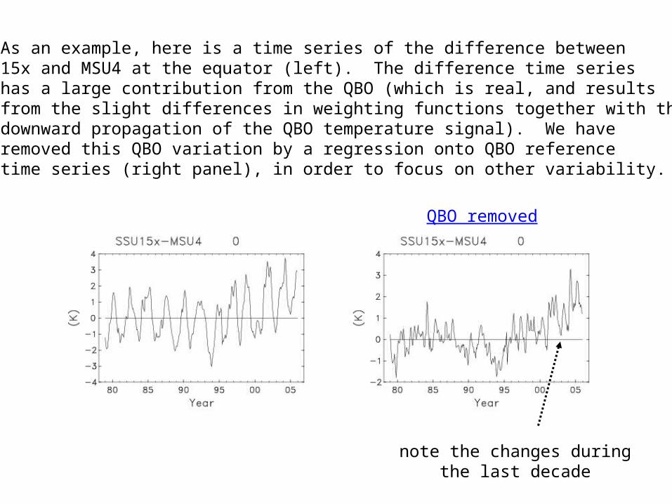
As an example, here is a time series of the difference between15x and MSU4 at the equator (left). The difference time series has a large contribution from the QBO (which is real, and results from the slight differences in weighting functions together with thedownward propagation of the QBO temperature signal). We have removed this QBO variation by a regression onto QBO reference time series (right panel), in order to focus on other variability.

QBO removed

note the changes duringthe last decade

We have generalized these calculations by performing an EOF analysis of thelatitude-time field of differencesfor 15x - MSU4. This is intended to capture dominant patterns of variability in the difference fields.The first EOF has a spatial patternthat maximizes in the tropics (top),with a time variation shown at bottom. (This mode captures 79% ofthe overall variance in the differencefields). The key point is that thetime series shows a discontinuousbehavior, with a trend during thelast decade.

It would take an unusual atmosphericstructure to generate this behaviorin reality.

Here’s a similar calculationfor 26x – 25. Again the timeseries (bottom) shows a trend at the end.

Likewise for 36x – 27. The timeseries (bottom) shows a trend at the end.

In summary, all of the difference fields between the x-channels and original channels are dominated by atime variation that is relatively flat for ~1979-1997, and then changes monotonically after 1998-2000. Thissuggests to me that something systematic is happening.

Recall that all of the x-channels are tied to channel 26.

The curious behavior of channel 26 seen in the time seriesand trends (in comparison with 25 and 27), together withthe systematic behavior seen in the x-channel difference fields, suggests to me that something may be amiss in the channel 26data for the most recent decade. Note this is the periodwhen the record is based on NOAA-14, and there is a significant orbit drift during this time.

Overall, I am suspicious of the detailed results derived fromchannel 26, and all of the x-channels, for the NOAA-14 period.

Some questions:

Is there anything suspicious about the NOAA-14 instrument (channel 26 in particular)?

Could this somehow be a tidal effect? The spatial structure of the difference fields peaks at the equator, and covers ~ 30 N-S (from the EOF spatial structure plots), and there are strongertides at the equator. But, why an influence on channel 26 andless on 25 and 27?

Any ideas from others?