space-time observations for city level air quality ...€¦ · ipsit dash enschede, the...
TRANSCRIPT

SPACE-TIME OBSERVATIONS
FOR CITY LEVEL AIR QUALITY
MODELLING AND MAPPING
IPSIT DASH
February, 2016
SUPERVISORS:
Dr. N.A.S. Hamm
Prof. Dr. Ir. A. Stein


SPACE-TIME OBSERVATIONS
FOR CITY LEVEL AIR QUALITY
MODELLING AND MAPPING
IPSIT DASH
Enschede, The Netherlands, February, 2016
Thesis submitted to the Faculty of Geo-Information Science and Earth
Observation of the University of Twente in partial fulfilment of the
requirements for the degree of Master of Science in Geo-information
Science and Earth Observation.
Specialization: Geoinformatics
SUPERVISORS:
Dr. N.A.S. Hamm
Prof. Dr. Ir. A. Stein
THESIS ASSESSMENT BOARD:
Prof. Dr. Ir. M.G. Vosselman (Chair)
Dr. Ir. G. Hoek (External Examiner, IRAS, Utrecht University)

DISCLAIMER
This document describes work undertaken as part of a programme of study at the Faculty of Geo-Information Science
and Earth Observation of the University of Twente. All views and opinions expressed therein remain the sole responsibility
of the author, and do not necessarily represent those of the Faculty.

i
ABSTRACT
Spatiotemporal characterization of ambient air quality in a city is an important issue from epidemiological
and regulatory standpoint. Observations in form of air quality model predictions and ground based
measurement networks can be integrated to model the space-time behaviour of pollutants such as particulate
matter and facilitate predictions at unmeasured locations. Prior using model predictions, it is imperative to
evaluate their performance against measurements while considering uncertainty levels associated in them.
This study firstly, assesses the prediction performance of PM10 and PM2.5 from a downscaled city level
dispersion model, URBIS against measurements from low cost sensor network ILM at different temporal
aggregation. This comparison is asserted by means of model performance criteria that includes various
statistical metrics and utilizes measurement uncertainty associated with the ILM network. Secondly, these
observations were integrated in a Bayesian maximum entropy framework to generate prediction maps of
PM10 and PM2.5 in Eindhoven at hourly and daily temporal resolutions. BME approach allowed
incorporation of these observations characterized by their uncertainty.
Results of performance evaluation shows that URBIS predictions were consistent with ILM measurements
at daily levels of aggregations. Furthermore, these predictions were found accurate at locations proximal to
traffic sources and were inconsistent at city background locations. These inconsistencies were attributed to
inadequacy in estimation of background concentration levels of PM in the URBIS. Utilization of mean ILM
measurements as background values led to substantial improvement in the prediction performance of
URBIS. Spatiotemporal maps from the BME integration were able to show the variability in concentration
levels in the city at different locations and time periods. Prediction accuracy of BME was evaluated using
leave-one-out cross validation method and were found acceptable for PM2.5 maps and moderate for PM10.
This research concludes that measurements from ILM can be integrated with URBIS for fine-scale mapping
of pollutants in the city.
Keywords: particulate matter, URBIS, ILM, BME

ii
ACKNOWLEDGEMENTS
First and foremost, I would like to thank the omnipotent omniscient and omnipresent God for always
lighting up my path and guiding me towards righteousness. I dedicate this research work to my parents
for their unconditional love, support and sacrifice. I would like to thank all my teachers for motivating
me by their exemplifying ideologies, be in through academics or experiences to help build up my
character, morale and thirst for knowledge.
This MSc would not have been possible without the blessings of Dr. Parth Sarathi Roy, Ex-Director,
Indian Institute of Remote Sensing, Dehradun whose inspiration motivated me to pursue my career in
Geoinformation Sciences. My sincere regards to Dr. C. Udhayakumar, Prof. R. Nagendra, Anna
University Chennai and Dr. Gyozo Gidofalvi, Dr. Takeshi Shirabe, KTH Royal Institute of Technology,
Sweden for their inspiring lectures that always infused in me a zeal to reason and question everything.
I am deeply indebted to my supervisors, Dr. Nicholas Hamm and Prof. Dr. Ir. Alfred Stein, who have
shaped my dream of being a young researcher. Their guidance and encouragement all through the
research period has been phenomenal. I feel greatly honoured to have been mentored by them and have
learnt a lot from their ideas, suggestions and constructive criticisms. I acknowledge my gratitude to Dr.
Hamm for sharing his expertise in the field of air quality modelling and his kind support without which
my research would not have been possible. I thank Prof. Stein especially for his introductory lecture in
the Spatial Data Quality module on 4th January 2015 which steered my enthusiasm toward this domain
of research.
I would like to thank Dr. Jan Duyzer, Mr. Sjoerd van Ratingen from TNO and Drs. Hans Berkhout,
from RIVM for their help in obtaining essential datasets needed for the research. I appreciate all the
fruitful discussions on air quality modelling with Vera van Zoest, Alfredo Gomez and Noshan Bhattrai
which also contributed towards the completion of my thesis. I thank Rahul Raj for his advice and his
motivation.
I am blessed to have made a wonderful spectrum of friends during my study at ITC. Their love and
affection has really supported me to complete my thesis. I really appreciate mental support of my GFM
colleagues and ITC amigos especially Rushikesh, Angela, Andreea, Amos, Noshan, Laura and Mirza
during my stay in the Netherlands.
Finally, last but certainly not the least, I would like to thank Sheilla Ayu Ramadhani, for being a friend,
philosopher and guide. I really acknowledge her crucial contribution in my life.

iii
“There is no such uncertainty as a sure thing” Robert Burns (1756-96)

iv

v
TABLE OF CONTENTS
List of figures ................................................................................................................................................................ vi
List of tables ................................................................................................................................................................. vii
List of acronyms ........................................................................................................................................................ viii
1. Introduction ........................................................................................................................................................... 1
1.1. Background and significance ................................................................................................................................. 1 1.2. Motivation and problem statement ...................................................................................................................... 2 1.3. Research identification ........................................................................................................................................... 4 1.4. Thesis structure ....................................................................................................................................................... 4
2. Literature review ................................................................................................................................................... 5
2.1. Air quality modelling .............................................................................................................................................. 5 2.2. Particulate matter in the Netherlands ................................................................................................................... 6 2.3. Performance evaluation of air quality models ..................................................................................................... 7 2.4. Bayesian maximum entropy method .................................................................................................................... 8
3. Study area and data ............................................................................................................................................ 11
3.1. Study area ............................................................................................................................................................... 11 3.2. Datasets description.............................................................................................................................................. 12
4. Methods ............................................................................................................................................................... 23
4.1. Evaluation of URBIS predictions against ILM measurements ....................................................................... 23 4.2. Data integration by Bayesian Maximum Entropy method .............................................................................. 27
5. Results and analysis ........................................................................................................................................... 33
5.1. Exploratory analysis .............................................................................................................................................. 33 5.2. Performance evaluation of URBIS Model ......................................................................................................... 37 5.3. Spatiotemporal prediction of PM values using BME ...................................................................................... 47 5.4. Comparison of mean ILM measurements with averaged LML for background PM .................................. 55
6. Discussion ........................................................................................................................................................... 59
7. Conclusions ........................................................................................................................................................ 63
7.1. Answer to research questions .............................................................................................................................. 63 7.2. Limitations and Recommendations .................................................................................................................... 65
List of references ........................................................................................................................................................ 67
Appendices .................................................................................................................................................................. 75
vi
LIST OF FIGURES
Figure 1 Municipality of Eindhoven and its constituent districts ....................................................................... 11
Figure 2 Population (left) and landuse (right) categorization in Eindhoven (CBS, 2016a) ............................. 11
Figure 3 Spatial representativeness of ILM network in Eindhoven ................................................................... 13
Figure 4 Specifications of PPD42NS Optical sensor (AQICN, 2016) ............................................................... 13
Figure 5 Schematic representation of HDF storage format of ILM measurement data ................................. 14
Figure 6 Schematic representation of URBIS dispersion model and its prediction process .......................... 16
Figure 7 Location of LML monitoring stations near Eindhoven ........................................................................ 19
Figure 8 Boxplots of PM10 (above); PM2.5 concentrations (below) at background LML stations ................. 20
Figure 9 Time series of PM10 measurements from LML background stations and averaged background .. 21
Figure 10 Time series of PM2.5 measurements from LML background stations and averaged background 21
Figure 11 Methodology for performance evaluation of URBIS model against ILM measurements ............ 26
Figure 12 Workflow of integration of URBIS predictions with ILM measurement data in BME ................ 29
Figure 13 Input data and prediction grid for BME analysis ................................................................................. 30
Figure 14 Airbox locations (ILM network) and corresponding URBIS prediction locations ........................ 33
Figure 15 Comparison of PM values from ILM, background LML and URBIS foreground predictions ... 34
Figure 16 Exploratory analysis of PM10 values at airbox locations ................................................................... 34
Figure 17 Exploratory analysis of PM2.5 values at airbox locations .................................................................. 34
Figure 18 Temporal visualization of ILM- PM10 values at 32 airbox locations for June 2015 ..................... 35
Figure 19 Temporal visualization of ILM- PM2.5 values at 32 airbox locations for June 2015 .................... 36
Figure 20 Temporal visualization of URBIS- PM10 values at 32 airbox locations for June 2015 ................. 36
Figure 21 Temporal visualization of URBIS- PM2.5 values at 32 airbox locations for June 2015 ................ 37
Figure 22 Principle of equal tolerance plots for hourly aggregations - PM2.5 .................................................. 43
Figure 23 Principle of equal tolerance plots for hourly aggregations - PM10 ................................................... 44
Figure 24 Principle of equal tolerance plots for daily aggregations - PM2.5 ..................................................... 45
Figure 25 Principle of equal tolerance plots for daily aggregations - PM10 ...................................................... 46
Figure 26 Covariance analysis for BME predictions of daily PM10. .................................................................. 47
Figure 27 Daily PM10 prediction maps in Eindhoven ......................................................................................... 48
Figure 28 Covariance analysis for BME predictions of daily PM2.5 .................................................................. 49
Figure 29 Daily PM2.5 prediction maps in Eindhoven ........................................................................................ 50
Figure 30 Covariance analysis for BME predictions of hourly PM10 ................................................................ 51
Figure 31 Hourly PM10 prediction maps in Eindhoven ...................................................................................... 52
Figure 32 Covariance analysis for BME predictions of hourly PM2.5 ............................................................... 53
Figure 33 Hourly PM2.5 prediction maps in Eindhoven ..................................................................................... 54
Figure 34 Timeseries of mean ILM values and averaged background from LML stations ............................ 55
Figure 35 Covariance analysis for BME predictions of daily PM2.5 (using ILM as background) ................. 56
Figure 36 Daily PM2.5 prediction maps in Eindhoven (using ILM as background) ....................................... 57
Figure 37 Principle of equal tolerance - daily aggregated PM2.5 (using ILM as background in URBIS
predictions) ................................................................................................................................................................... 58

vii
LIST OF TABLES
Table 1 PM10 and PM2.5 measurements from airboxes used in research ........................................................... 12
Table 2 Brief description of ILM dataset ............................................................................................................... 14
Table 3 Discussions on data quality of ILM measurements ................................................................................ 15
Table 4 Brief description of URBIS dataset ........................................................................................................... 17
Table 5 Discussions on data quality of URBIS model predictions .................................................................... 17
Table 6 Description of LML stations near Eindhoven ........................................................................................ 19
Table 7 Summary statistics of hourly PM values from LML stations ................................................................ 20
Table 8 Model performance criteria based on RMSE values (Thunis et al., 2012a) ........................................ 25
Table 9 Model performance criteria matrix for evaluation of URBIS predictions(Thunis et al., 2012a) ..... 25
Table 10 Levels of aggregation of URBIS predictions and ILM measurements .............................................. 26
Table 11 Site specific knowledge base (S-KB) for BME analysis ....................................................................... 30
Table 12 Summary statistics of PM values from ILM, background LML and URBIS foreground .............. 34
Table 13 Representative airbox locations for analysis .......................................................................................... 38
Table 14 MPC results at five representative stations for hourly aggregations .................................................. 38
Table 15 MPC results at five representative stations for 6-hourly aggregations .............................................. 38
Table 16 MPC results at five representative stations for 12-hourly aggregations ............................................ 39
Table 17 MPC results at five representative stations for daily aggregations ..................................................... 39
Table 18 Estimates of empirical covariance functions- daily PM10 BME analysis ......................................... 47
Table 19 Parameters for fitting nested covariance model- daily PM10 BME analysis .................................... 48
Table 20 Estimates of empirical covariance functions- daily PM2.5 BME analysis ........................................ 49
Table 21 Parameters for fitting nested covariance model- daily PM2.5 BME analysis ................................... 49
Table 22 Cross validation results- daily predictions BME ................................................................................... 50
Table 23 Estimates of empirical covariance functions- hourly PM10 BME analysis ...................................... 51
Table 24 Parameters for fitting nested covariance model– hourly PM10 BME analysis ................................ 51
Table 25 Estimates of empirical covariance functions- hourly PM2.5 BME analysis ..................................... 53
Table 26 Parameters for fitting nested covariance model- hourly PM2.5 BME analysis ................................ 53
Table 27 Cross validation results- hourly predictions BME ................................................................................ 54
Table 28 Estimates of empirical covariance functions- Daily PM2.5 BME analysis (using ILM as
background) ................................................................................................................................................................. 56
Table 29 Parameters for fitting nested covariance model– Daily PM2.5 BME analysis (using ILM as
background) ................................................................................................................................................................. 56
Table 30 Appendix 1: Measurement uncertainty in the ILM .............................................................................. 75
Table 31 Appendix 2: Daily PM10 maps in Eindhoven ...................................................................................... 77
Table 32 Appendix 3 -Daily PM2.5 maps in Eindhoven ..................................................................................... 78
Table 33 Appendix 4-Hourly PM10 maps for June 04 in Eindhoven ............................................................... 79
Table 34 Appendix 5 - Hourly PM2.5 maps for June 04 in Eindhoven ............................................................ 80

viii
LIST OF ACRONYMS
PM Particulate matter
PM10 Particulate matter with aerodynamic diameter less than 10 μg m-3
PM2.5 Particulate matter with aerodynamic diameter less than 2.5 μg m-3
UFPs Ultrafine particles
ILM Innovatief luchtmeetsysteem (Innovative air measurement system)
URBIS Urban information system
MPC Model performance criteria
BME Bayesian maximum entropy
RMSE Root mean square error
NMB Normalized mean bias
NMSD Normalized mean standard deviation
R Correlation coefficient

SPACE-TIME OBSERVATIONS FOR CITY LEVEL AIR QUALITY MODELLING AND MAPPING
1
1. INTRODUCTION
1.1. Background and significance
Clean air is a key requirement for human health. As a consequence of numerous anthropogenic activities
and physical processes, various pollutants are introduced in the atmosphere, altering the optimal
composition of air. These pollutants in the form of gases and particulates of organic and inorganic origin
lead to health effects and environmental deterioration. Epidemiological studies have explained the causality
of human morbidity and mortality with exposure to polluted air (Brunekreef & Holgate, 2002). Similarly
environmental degradation caused by eutrophication, acid rain, smog and climate change have been linked
with air pollution (Colls & Tiwary, 2009; Lazaridis, 2011). This has led to an increased interest in
understanding the process behind air pollution and developing strategies for its sustainable mitigation.
Air pollutants of concern for human health can be classified into six classes (EEA, 2015c; EPA, 2015) These
are oxides of nitrogen (NOx) formed as combination of nitrogen dioxide (NO2)and nitrous oxide (NO),
ozone (O3), particulate matter (PM), carbon monoxide (CO), sulphur dioxide (SO2) and lead (Pb). Amongst
these, health risks associated with exposure to particulate matter (PM) are of significant concern, especially
given increases in cardiovascular and respiratory disease (Bernard et al., 2001; Kim et al., 2015; Murad, 2012;
Shah et al., 2013). Exposure to PM poses a major immediate threat for pregnant women, resulting in
increased chances of autism spectrum disorder in offspring (Raz et al., 2014). It also causes health risks in
elderly (Liu et al., 2009) and young children (Yip et al., 2004).
PM varies in chemical composition and size. These are composed of non-organic nitrate and sulphate rich
secondary aerosols, organic carbon compounds like polycyclic aromatic hydrocarbons (PAH) and metal
traces (WHO, 2013). These are generated primarily from transportation (vehicular exhaust, wear and tear of
roads, brakes and tyres) and industrial combustion processes (Visser et al., 2001). Secondary sources of PM
include those from agriculture (nitrogenous emissions, tillage operations, fertilizers and pesticides),
construction (dust particles, paints) and mining (mineral dust, inorganic particulates) (Araujo et al., 2014;
Arslan & Aybek, 2012; Juda-Rezler et al., 2011).
PM it is categorized according to its aerodynamic diameter. This categorization is based on different factors
such as correlation of size of PM with its gravimetric mass, ability to transport in the atmosphere and level
of penetration into human respiratory system (Kim et al., 2015). Thus different categorizes of PM are coarse
particulate matter (PM10) with aerodynamic diameter of less than 10 μg m-3, fine particulate matter (PM2.5)
with aerodynamic diameter of less than 2.5 μg m-3 and ultra-fine particulate matter (UFPs) with aerodynamic
diameter less than 0.1 μg m-3 (US-EPA, 2015).PM10, depending upon local meteorological conditions tend
to stay in the atmosphere from few minutes to hours and has movement of few meters to kilometres from
emission source to deposition. PM2.5 generally remain suspended in the atmosphere for few days and have
movement in range of few to hundreds of kilometres. UFPs tend to remain in the atmosphere for few days
to weeks in and are most susceptible to fluctuations in meteorological conditions (Cheung et al., 2011;
Srimuruganandam & Shiva Nagendra, 2012).
In recent years, there has been an increased focus for regulating emission levels to improve air quality. Air
quality guidelines mandated by the World Health Organization (WHO, 2006) act as a global standard while
these are also set by national bodies such as NAAQS (national ambient air quality standards ) for U.S.A.
SPACE-TIME OBSERVATIONS FOR CITY LEVEL AIR QUALITY MODELLING AND MAPPING
2
(EPA, 2015), air quality directives for EU (European Union) member states (EU, 2008). In Europe, annual
average for PM10 values should not exceed 40 μg m-3 and daily average should not exceed 50 μg m-3 with 35
allowable exceedances cases per year. These values are set according to the guidelines of air quality directives
and should be obtained by 2005 for all member states (EEA, 2014b; EU, 2008). Similarly, the allowable
mean limit values for PM2.5 should be less than 25 μg m-3 achievable by 2015 (Matthijsen & ten Brink, 2007).
Proper enforcement of these regulations require correct determination of PM (PM10 and PM2.5) values in
space and time and are obtained by means of air quality measurements or as predictions from air quality
models. Air quality modelling, in general involves combining information of atmospheric behaviour of
pollutants with observations to model spatiotemporal characteristics of pollutant and provide predictions in
space and time. Predictions from these models can be used to characterize emission sources, quantify their
contributions and develop pollution reduction strategies. These models differ at various spatiotemporal
scales and also on underlying principles of modelling. City-level air quality models are of particular
importance as their predictions have substantial implications on local governance strategies such as
monitoring adherence to defined emissions protocols, health studies and sustainable urban planning policies
(Chang & Hanna, 2004).
1.2. Motivation and problem statement
The behaviour of PM is dynamic in the atmosphere. The concentration and chemical composition does not
remain constant over a particular region at a particular time (Yadav et al., 2014). Concentration levels of PM
in space and time are measured at ground based stations mainly by semi-continuous automated methods
based on mass measurements (like beta attenuation monitors (BAM), filter based gravimetric samplers or
tapered element oscillating microbalance (TEOM) or by continuous method such as optical sensors that
correlate particle counts with gravimetric mass (EU, 2010; Williams & Bruckmann, 2002). It is only possible
to take measurements at a limited number of locations. In order to obtain values at unmeasured locations,
modelling is necessary. Air quality models facilitate low cost assessment of air quality by providing
predictions for a continuous geographic region and can augment existing ground based measurement
network.
Air quality models simulate the behaviour of pollutants in space and time and thus their predictions may be
imperfect (Borrego et al., 2008) and associated with a relevant amount of uncertainty. Uncertainties
associated in modelling can be due to inadequate representation of sources, errors in modelling procedures,
errors associated with input data such as instrument errors and the spatiotemporal variability of PM10 in
atmosphere (Riccio et al., 2006) might lead to incorrect representation of pollutant. A near-ideal model
would be that which represents adequately the spatiotemporal variability of a pollutant and predicts with a
minimal amount of quantifiable uncertainty. Furthermore, formulation of air quality models are dependent
on input data, their spatial resolution and temporal frequency. Models designed for predicting air quality
such as at city-level require input data at a finer spatiotemporal scale and thus needs to overcome input data
scarcity.
Following developments in micro-electrical mechanical systems (MEMs), the availability of cost effective
and reliable sensors have become increasingly popular in urban air quality monitoring (Kumar et al., 2015).
These distributed system of sensor networks, relying on the state-of-the-art wireless transmission
infrastructure can be used for pollutant measurements in near-real time and overcome the observational
data scarcity. These measurements can be utilized to support real time assessment of exceedance levels and
can be used as input data in air quality models for predicting concentration levels at unmeasured locations
(Knox et al., 2013). In Eindhoven, AiREAS initiative (AiREAS, 2014; Close et al., 2016) has set up a low-
cost sensor network ILM (Innovatief Luchtmeetsysteem) since 2013. This network measures pollutants like

SPACE-TIME OBSERVATIONS FOR CITY LEVEL AIR QUALITY MODELLING AND MAPPING
3
PM, UFPs, O3, oxides of nitrogen and meteorological information like temperature and relative humidity at
35 locations (airboxes) spread across the city for every 10 minute interval and are made available in real-time
in an online repository (Hamm et al., 2016).
In the Netherlands, to predict pollutant levels in a city, an urban-scale air quality model- Urban Information
System (URBIS) (Beelen et al., 2010; Duyzer et al., 2015; Fritz & Borst, 1999) is also used. It is developed
and maintained by Nederlandese Organisatie voor Toegepast Natuurwetenschappelijk Onderzoek (TNO)
translated as (Netherlands organisation for applied scientific research) (TNO, 2015). URBIS takes into
account emissions from various stationary sources (like industries, residential areas and construction sites),
non-stationary sources (like traffic in highways and street canyons) and uses an ensemble of dispersion
models to provide mean predictions of pollutants like PM (PM10, PM2.5), O3, NOx at a yearly basis. In order
to use these predictions for augmenting pollution reduction strategies through continuous monitoring,
URBIS predictions are downscaled to finer temporal scales such as hourly values.
Integration of predictions from downscaled URBIS model and continuous measurements from ILM
network can facilitate an improved understanding of spatiotemporal variability of PM (PM10 and PM2.5) in
Eindhoven. However, to use predictions from URBIS model with confidence, it is important to evaluate its
performance accuracy. Measurements from the ILM network can be used to evaluate accuracy of URBIS
model predictions and can give an overview its performance by employing a number of statistical indicators
Statistical evaluation of air quality models is considered as one of the key methods to assess the accuracy of
predictions relative to measured values. Multiple statistical indicators such as root mean square error
(RMSE), bias, standard deviation, correlation coefficient have been recommended for evaluation of air
quality models. (Borrego et al., 2008). Nonetheless, it is also imperative to consider the uncertainty associated
with the PM measurements in the ILM network as the first step for an unbiased evaluation of model
accuracy. Limits of measurement uncertainties of pollutants by instruments are generally standardized in the
air quality directives with adherence to specific data quality objectives. (Pernigotti et al., 2013). For instance
in Europe, relative uncertainty associated with PM is set at 25% around the mean daily values of
measurement, whilst that for O3 is 15% around mean 8-hourly values and NO2 remains 15% for hourly
values (EU, 2010; Thunis et al., 2012a). These are representative standards and actual values depends upon
instrument used and on reference time period. Thus URBIS predictions can be evaluated against ILM
measurements taking into consideration different statistical indicators standardized by measurement
uncertainty of ILM network before its integration.
Modern geostatistical methods like spatiotemporal kriging, can predict concentration levels in with
associated prediction error variance that quantifies its uncertainty (Gräler et al., 2012; Knotters et al., 2010).
Bayesian maximum entropy (BME) is one such hybrid approach which can be used to model pollutants in
a stochastic space-time framework (Christakos & Serre, 2000; Christakos, 1990; Serre & Christakos, 1999).
BME formulates on an epistemic knowledge synthesis, taking into account available information to
characterize the space-time dependence structure of pollutant and integrates with data from multiple sources
to predict concentration levels. It has the ability to incorporate soft data (data with quantified uncertainty in
its value) with hard data (data with negligible amount of uncertainty associated with its values) as input and
estimates the concentration levels for requisite geographical area and temporal range. Prediction at each
location is associated with a probability distribution function which leads to better quantification of
estimation uncertainty, in terms of error variances, occurrence probabilities, confidence levels (Pang et al.,
2009). Quantification of uncertainty in pollutant concentration estimates is of particular importance for
decision makers for applications while assessing exceedance levels and human exposure. Predictions from
URBIS can be integrated with ILM measurements in a BME framework to produce spatiotemporal maps
of PM levels (PM10 and PM2.5) in Eindhoven that can facilitate continuous monitoring of air quality.

SPACE-TIME OBSERVATIONS FOR CITY LEVEL AIR QUALITY MODELLING AND MAPPING
4
1.3. Research identification
There are two aspects to this research. Firstly, to evaluate PM predictions (PM10 and PM2.5) of URBIS, by
using a set of quantitative statistical indicators, against ILM measurements. Uncertainty associated with ILM
measurements is utilized in these statistical indicators. This is to determine, given a threshold uncertainty
level in ILM measurements how efficient is the URBIS model in constraining this uncertainty in its
predictions.
Secondly, to utilize BME to integrate ILM measurements and predictions from URBIS dispersion model to
map spatiotemporal variability of PM in Eindhoven region. The motivation is to compare the prediction of
the integrated model against independent measurements and assess the feasibility of using low cost sensor
network to augment prediction.
1.3.1. Research objectives
Based on the domain of research identified, the following are the objectives of this research:
1. Statistical evaluation of PM predictions (PM10 and PM2.5) from the URBIS model against PM
measurements from the ILM network using allowable limits of measurement uncertainty.
2. Integration of data from ILM network and URBIS model predictions in a BME framework to map
spatiotemporal variability of PM (PM10 and PM2.5) in Eindhoven.
1.3.2. Research questions
Questions related to objective 1:
a) What are the key statistical indicators that are needed to evaluate URBIS model?
b) How to formulate and interpret model performance criteria (MPC) to evaluate URBIS model based
on statistical indicators and measurement uncertainty of ILM network?
c) What are suitable space-time scales for representing PM concentration levels?
Questions related to objective 2:
a) Which data should be considered as soft (data with uncertainty) and hard (certain data)?
b) How to model the space-time dependence of PM?
c) How to integrate space-time dependence of PM with available data from URBIS model and ILM
measurements to generate prediction maps?
d) How can the accuracy of BME process be assessed?
1.3.3. Innovations aimed at
1. Defining model evaluation criteria of PM predictions from the URBIS model against measurements
from the ILM network at different temporal scales.
2. Integration of ILM measurements with URBIS model predictions in a BME framework for
spatiotemporal mapping of PM in Eindhoven.
1.4. Thesis structure
Chapter 1 gives the rationale of the study and details the research objectives and underlining research
questions that are intended to be addressed in the thesis. Chapter 2 gives a detailed review of the literature
pertaining to air quality model evaluation and application of BME in air quality modelling. Chapter 3
describes the study area and the datasets used in the research and Chapter 4 gives a conceptual framework
and workflow of methods involved. Results and analysis are presented in Chapter 5. Chapter 6 includes
discussions of the results. Chapter 7 summarizes the study and deals with conclusions, limitations and
recommendations.

SPACE-TIME OBSERVATIONS FOR CITY LEVEL AIR QUALITY MODELLING AND MAPPING
5
2. LITERATURE REVIEW
2.1. Air quality modelling
Jerrett et al., (2005) reviewed and categorized six different classes of air quality models based on their
underlining modelling procedure and assessed their credibility in measuring exposure levels in Hamilton,
Canada. These were: proximity models, dispersion models, spatial interpolation models, land use regression
models and integrated meteorological-emission models. Proximity based models generally predict
concentration levels based on nearness to emission source. These predictions are reliable near pollution
sources but tend to be uncertain at non-proximal locations. Land use regression models require an optimal
selection of predictor variables for plausible predictions. Spatial interpolation models can be affected by
sparse input observations and may produce erroneous results. Regional chemical transport models (CTMs),
which take into consideration various meteorological factors and chemical composition of pollutants in
atmosphere, tend to deliver predictions at rather coarser resolution that limits its credibility to predict subtle
spatial variations such as in a city. Their studies concluded that improvisation in input data and combination
of more than one modelling methods tend to increase accuracy of predictions
Daly & Zannetti, (2007) discussed the effectiveness of dispersion models and photochemical models in
simulating the behaviour of pollutants in the atmosphere. They explained the behaviour of a pollutant after
its emissions in atmosphere is governed by processes of dispersion, transportation, chemical alteration and
finally ground deposition. Dispersion models, which tend to model emissions to deposition of pollutant are
categorized as Lagrangian models which and Eulerian models based on their interpretation of atmospheric
interaction. Whilst Eulerian model divides atmosphere into grids and simulate the behaviour of pollutant at
each grid, Lagrangian model consider trajectory of pollutant as an air parcel and simulate its behaviour in
space and time.(Nielinger et al., 2004). Photochemical models take into consideration the physical and
chemical transformation of a pollutant in the atmosphere and simulate its behaviour. Facilitating low-cost
assessment of air quality, these models are preferred for larger geographical regions like national or global
level. Nguyen, (2014) reviewed dispersion models, photochemical models and receptor models on the basis
of their input data, modelling procedures and probable applications. Receptor models employ series of
statistical and mathematical processes to elucidate contributions of different sources of pollution at receptor
locations.
Landuse regression models (LUR) have been used to link air quality modelling with human exposures. Ryan
& LeMasters, (2007) mentioned four classes of predictor variables that were mostly influential for
concentration levels. These were, type of road, traffic counts, elevation and land cover of which traffic
count. Beelen et al., (2010) compared the performances of LUR to that of URBIS model in yearly predictions
of NO2 in Rijnmond area in Rotterdam, the Netherlands. They concluded that predictions from URBIS
model explained intra-urban small-scale variability better than that of LUR. Studies by de Hoogh et al.,
(2013); Hoek et al., (2008) gives an understanding about developments of LUR models and its applications
in human exposure studies in European cities. Alam & McNabola, (2015) studied the usage of multiple
linear regression models in predicting daily levels of PM10 at Vienna and Dublin and were able to
demonstrate the effectiveness of LUR in providing consistency in model predictions over time. Wang et al.,
(2014) developed LURs for NO2 and PM at continental and regional scales and reported that these LURs
provided reasonably good predictions where monitoring stations were absent.
Spatiotemporal interpolation methods used widely in environmental modelling purposes (Li & Heap, 2011,
2014) have also been implemented for air quality studies. Geostatistical methods such as spatiotemporal

SPACE-TIME OBSERVATIONS FOR CITY LEVEL AIR QUALITY MODELLING AND MAPPING
6
kriging, take into account the correlation in space and time of pollutant observation and use it to model
predictions at unknown locations. It relies on similarity in air pollutant characteristics governed by its
spatiotemporal structure and can be explained by Tobler’s law of geography “everything is related to everything
else, but near things are more related than distant things” (Miller, 2004; Tobler, 1970). Wong et al., (2004) utilized
four different methods such as spatial averaging, nearest neighbourhood, IDW and spatial interpolation
method of ordinary kriging to predict PM10 and O3 concentrations in the U.S. and explained the
effectiveness of these methods in air quality predictions. Authors reported that kriging provided optimal
results with relatively scarce monitoring data. Real-time modelling of air quality was done by Janssen et al.,
(2008) using measurements and landuse information from CORINE dataset by means of a de-trended
kriging model for prediction of pollutants such as O3, PM10 and NO2 in Belgium. Jha et al., (2011) appraised
various interpolation techniques for predicting suspended particulate matter (SPM), sulphur dioxide (SO2)
and nitrogen dioxide (NO2) in Port Blair, India and reported that these methods are suitable for prediction
when a scarce amount of input data is available.
Hybrid models employ an integrated approach of using two or more modelling frameworks to improvise
the prediction abilities by overcoming weakness of individual modelling techniques (Hamm et al 2015).
Akita et al.,( 2014) demonstrated the effectiveness of discerning intra-urban exposure variability by
integrating results of land use regression model and output of chemical transport model in a BME
framework. The overall accuracy was higher as compared to individual accuracies of land use regression
model or that of chemical transport model. Similar works by Beckerman et al., (2013); Li et al., (2013) also
demonstrates the capability of hybrid air quality models for estimating concentration of pollutants with
improved accuracy. Works by van de Kassteele et al., (2009); van de Kassteele & Stein, (2006) combined air
quality measurements and output from dispersion model by means of external drift kriging (KED) in an
Bayesian framework to predict NO2 in the Netherlands. They were successful in demonstrating the use of
KED as a suitable interpolation method and ability to combine different data sources in improvising the
predictions. Hamm et al., (2015) utilized a spatially varying coefficient geostatistical (SVC) model to map
PM10 in central, south and eastern Europe using measurement data from Airbase network (EEA, 2014c)
and regional CTM LOTOS-EUROS (Schaap et al., 2008). Authors concluded that SVC model predictions
could be used for mapping exceedance levels of PM10 and also to evaluate the performance of LOTOS-
EUROS model.
2.2. Particulate matter in the Netherlands
Matthijsen & Koelemeijer, (2010) showed that anthropogenic sources contributing to PM10 and PM2.5 in the
Netherlands compose of secondary aerosol formation (including sulphates, nitrates, ammonia, volatile
organic compounds, and mineral dust). By implementation of proper policy measures of reducing emissions
of secondary aerosols into the atmosphere, considerable amount of reduction in PM levels is expected.
Additionally, contribution of sea salt to PM10 and PM2.5 levels are 12% and 5% respectively. Emissions from
road traffic also account towards contribution to PM2.5 and elemental carbon (EC), however PM is majorly
dominated by background concentrations. According to Matthijsen & ten Brink, (2007) current annual
regional background concentrations of PM2.5 range between 12-16 μg m-3 while urban background
concentration are in range of 16-18 μg m-3. Additional increments from the streets predominantly due to
traffic lies between 2-6 μg m-3 while that for highways lies in range of 7-14 μg m-3. VROM, (2008) also
reported that major contributions of PM10 in the Netherlands were results from non-anthropogenic sources
and from transboundary anthropogenic emissions that dominated local level contributions to PM10.
Even though with stringent European Union policy of using low exhaust vehicles (Euro Standards: light-
duty vehicles are Euro V/Euro VI and heavy-duty vehicles are Euro IV (EEA, 2015b)) has led to decrease
in PM levels from exhaust emissions, but with increase in traffic count, contribution from non-exhaust

SPACE-TIME OBSERVATIONS FOR CITY LEVEL AIR QUALITY MODELLING AND MAPPING
7
sources like brake wear and tear, tyres, road wears still contribute to the levels of PM. This has also been
concluded by studies of Boogaard et al., (2011) wherein high contrasts were found in concentration levels
of coarse PM components (Chromium, Copper and Iron), particle number concentrations (PNCs) and black
carbon while comparing eight major roadways and nine sub-urban background stations. Keuken et al.,
(2011) conducted a health impact assessment of PM10 and elemental carbon (EC) in Rotterdam by studying
the trends in concentration levels and life expectancies for 1985-2008 and concluded that increasing traffic
count with efficient vehicular combustion have led to overall decrease emissions. Furthermore, decrease in
industrial emissions by stricter regulations and stringent urban planning policies, air quality has improved
with decrease of averaged urban PM10 background concentration from 43 μg m-3 (1985) to 25 μg m-3 (2008)
and has resulted in considerable gain life expectancy (for PM10).
Hoogerbrugge et al., (2010) reported that average annual concentration of PM10 resulting from
anthropogenic sources have reduced considerably since 1990-2000. Approximately two thirds of the
decrease was due to reduction in emissions of sulphates and nitrates from anthropogenic sources and
remaining from primary vehicle exhausts and secondary aerosols. European Environmental Agency (EEA,
2014a, 2015a) reported that there has been a reduction in the yearly average levels of PM10 and PM2.5 for the
Netherlands. Estimate exposure levels to daily limiting values of PM10 (as set by European Union Air Quality
Directives (EU, 2008) of 50 μg m-3) was 0.5% approximately for urban population in 2010 which had
increased to 2.9% in 2011 and reduced to 0% by 2012.
2.3. Performance evaluation of air quality models
A detailed discussion on quantitative methods for assessing performance of model predictions to
measurements was presented by Bencala & Seinfeld, (1979). Performance of an air quality model can be
described broadly in terms of model validity, which refers to the ability of a model to replicate behaviour of
a pollutant in atmosphere and model accuracy, which refers to the correctness of model outcome. These
methods were based on analysis of residuals (difference in measured concentration and predicted
concentration at a particular location and time), analysis of model-measurement agreements including
correlation coefficient and linear least square fit and were part of a FORTRAN based performance
assessment package called “AQMAAP”.
Three major sources of uncertainties can be accounted while evaluating predictions of an air quality model
to that of measurements. They are namely, comparison of volume average predictions, generally given by
an air quality model to that of point measurements; instrument errors associated with measurements, wrong
input parameters and incorrect modelling techniques. MacKay & Bornstein, (1982) presented both
quantitative and qualitative methods of evaluating air quality simulation models. The quantitative methods
were basic statistical indicators like model bias, gross errors, noise and correlation coefficient defined around
pairs of model predictions and observations. Qualitatively, histograms and cumulative frequency plots were
favoured by the authors to depict the residuals while isopleths and time-series plots were argued suitable for
spatial correlation and temporal correlation respectively. Evaluating two or more air quality models by a
composite performance indicator based on aggregating fractional bias and absolute fractional bias was
recommended by Cox & Tikvart, (1990).
Chang & Hanna, (2004), reviewed various qualitative and quantitative methods for model evaluation. The
authors urge the use of multiple evaluation methods to assess the performance. Apart from discussing about
statistical parameters like root mean square error, fractional bias, geometric mean bias, normalized mean
square error, geometric variance, correlation coefficient and fraction of predictions within a factor of two
of observations, they discussed on qualitative performance indices like Taylor’s nomogram method (which

SPACE-TIME OBSERVATIONS FOR CITY LEVEL AIR QUALITY MODELLING AND MAPPING
8
combines normalized standard deviation, normalized root mean square error and correlation coefficient in
a single plot), figure of merit in space (ratio of prediction and observation contour area based on a certain
threshold) and cumulative distribution function method.
Boylan & Russell, (2006) considered evaluation of air quality models by using model bias (measure of
model’s over or under-prediction) and model error (measure of deviance of a model’s predictions to
observations). Similar works have been carried out in Tessum et al., (2015); Thi et al., (2012) wherein
evaluation of chemical transport model (CTM) predictions and dispersion model output against
measurements based on statistical parameters has been done. Bennett et al., (2013) characterised
environmental model performance and also explained various statistical, graphical and qualitative methods
for evaluating model output which can be utilized in air quality domain. Borrego et al., (2008), studied
different aspects of estimating uncertainty of model predictions and discussed several statistical metrics that
can be used for evaluation of performance of air quality model predictions against measurement data.
Air quality model evaluation can be differentiated into multiple components involving scientific evaluation
(ability of model to incorporate different emission sources and behaviour of a pollutant in atmosphere),
code verification (interpretation of processes as sound mathematical and physical expressions), model
accuracy (ability of model to predict concentration levels which coincides with observations) and sensitivity
analysis (checking the sub-models for their effectiveness) (Borrego et al., 2008; Chang & Hanna, 2004).
Statistical evaluation plays an important role in concluding whether a model is able to replicate the
concentration levels based on observed data. It can be considered as a crucial step to determine the
effectiveness of a model for a particular application.
Evaluating model predictions against reference data can give credible results if the reference data are error-
free. However, both model predictions and measurement data are associated with some degree of
uncertainty. These uncertainties in modelling and measurements can be attributed to different sources, such
as model might be wrongly formulated or has incorrect input parameters, while measurements may be
uncertain due to instrument errors (Borrego et al., 2008; Chang & Hanna, 2004). Thus prior to statistical
evaluation of model predictions against measurements, it is important to ascertain the uncertainty in
measurement data. This can help in determining how well modelled predictions are against given
measurement data and how accurately the model predicts pollutant value, whose actual value might lie
between the intervals of measurement data uncertainty. Thunis et al., (2012), proposed a model performance
criteria (MPC) that utilizes measurement data uncertainty in these statistical parameters for evaluating air
quality model performance. Furthermore, by utilization of various graphical tools like target diagrams, a
better insight into model performance can be achieved which can be used by decision makers to see explicitly
in which geographical area and time period the model performed well or badly. In works of Pernigotti et al.,
(2013); Thunis et al., (2013) these aspects of model evaluation were addressed specifically for pollutants like
ozone (O3), particulate matter (PM) and nitrogen dioxide (NO2). Riccio et al., (2006); Romanowicz et al.,
(2000) successfully demonstrated uncertainty evaluation for air quality models using a stochastic perspective
in a Bayesian framework.
2.4. Bayesian maximum entropy method
Bayesian maximum entropy (BME), detailed by Christakos, (1998) is a spatiotemporal interpolation method
that incorporates holistic information about any environmental phenomena (regarded as knowledge base)
by considering all available information about it, be it from its physical or chemical behaviour, variations in
space and time (regarded as general-knowledge base) and from available data from different sources such as

SPACE-TIME OBSERVATIONS FOR CITY LEVEL AIR QUALITY MODELLING AND MAPPING
9
observations or modelled predictions (regarded as site specific-knowledge base). Author especially
highlighted its applicability in cases where limited credible data (termed as hard data) is available, BME
facilitates usage of quantified uncertain data (or soft data) in augmenting process of interpolation. In limiting
cases BME can be considered similar to spatiotemporal kriging and is also flexible to operate in space-
only/time-only domains. Explanation about BME process is presented in details in works of Christakos,
Bogaert, & Serre, (2002); Kanevski, (2010). Serre & Christakos, (1999) applied the context of BME to study
the water-level elevations of “eqqus bed” aquifers in Kansas and concluded that incorporation of uncertain
(soft) data as input with measurement observation (hard data) leads to better accuracy in estimation.
Christakos & Serre, (2000) studied the spatiotemporal distribution of PM10 across North Carolina, United
States using BME analysis and concluded that kriging can be considered as a limiting case of BME, and that
BME framework facilitates increased flexibility in parameter estimation leading to improved characterization
of spatiotemporal variability. Nazelle et al., (2010) used BME approach to predict the concentration of 8-
hour O3 in North Carolina with improved accuracy and precision. They also demonstrated the flexibility of
BME method over other modern geostatistical interpolation methods like Bayesian melding. Similar results
were presented by Lee et al., (2008) as a synthetic case study, wherein proportion of increased soft data input
led to decrease in mean square error of the model predictions. The authors, by using BME were able to
improve accuracy in mapping minimum temperature of an urban heat island and demonstrated ability of
BME to incorporate soft data. Beckerman et al., (2013) utilized a hybrid model taking into consideration
remote sensing data, LUR and Bayesian maximum entropy (BME) methodology to study the spatiotemporal
variability of PM2.5 in the U.S. The employed BME interpolated predictions were more accurate than the
LUR method or remote sensing predictions alone. Similar work by Akita et al., (2014) involved usage of a
BME framework to integrate outputs from a dispersion model, LUR model and observation data for intra-
city exposure variability of NO2 half yearly concentration predictions and was able to evaluate that the hybrid
model performs better than any individual methods alone Study done by Adam-poupart et al., (2014) on
spatiotemporal modelling of O3 in Quebec, Canada investigated three methods of predictions namely, LUR
modelling, kriging and integrated the output of LUR and kriging in a BME framework and reported that
the predictions from the integrated method were the most accurate.


SPACE-TIME OBSERVATIONS FOR CITY LEVEL AIR QUALITY MODELLING AND MAPPING
11
3. STUDY AREA AND DATA
3.1. Study area
The study area is the city of Eindhoven (Figure 1). It spans from (51.40° N, 5.40° E) to (51.49° N, 5.53° E)
and is one of the major cities in the Netherlands. Figure 2 (left) is a bar chart showing the population
distribution according to different age groups and Figure 2 (right) shows landuse categories in Eindhoven
and their proportions (CBS, 2016b).
Figure 1 Municipality of Eindhoven and its constituent districts
Figure 2 Population (left) and landuse (right) categorization in Eindhoven (CBS, 2016a)

SPACE-TIME OBSERVATIONS FOR CITY LEVEL AIR QUALITY MODELLING AND MAPPING
12
Eindhoven houses 224,855 residents (November 2015) with average population density of 2.5 per km2. It
consists of 7 districts and has total surface area of 8,887 hectares. Approximately one third area of
Eindhoven comprises of residential units and other built up regions and has relatively lower area of greenery.
Majority of population resides in district Wossel- Noord (64,405 inhabitants) and least number of
inhabitants reside in Centrum district (6565 inhabitants). A distinct share of population belongs to age group
of 25-44 and 15-24 and can be attributed to majorly students and working professionals. Majority of
industries in Eindhoven are located in districts of Gestel and Strijp, with some of the industries located in
northern regions of district Woensel-Noord.
The A2 motorway passes through Eindhoven across the district of Strijp and along district Gestel.
Furthermore, road N2 (randweg) forms a beltways around the western border of Eindhoven and consists
of motorways A50 and A2. Motorway A270/N270, connects Helmond area with Tongelre district of
Eindhoven. These three motorways have potential influence on the PM emissions. Eindhoven airport and
aviation base are located in the western part of the municipality (district Strijp), and also contribute to the
emission of PM.
3.2. Datasets description
3.2.1. AiREAS initiative- ILM
During recent years, as a strive for clean air and healthy city, a low cost sensor network for measuring air
quality has been set up called- ILM (Innovatief Luchtmeetsysteem) translated as “Innovative air
measurement system” and operational (AiREAS, 2014; Close et al., 2016). It is a joint initiative of
municipality of Eindhoven with University of Utrecht and University of Twente, ECN, Philips and
Axians/Imtech ICT. There are currently 35 airboxes operating in and around Eindhoven which give
information about local air quality (particulate matter- PM10, PM2.5, PM1, UFPs, O3, and NO2) and
meteorology (relative humidity, temperature). This is the basis of ILM network. These data are obtained by
respective pollutant sensors installed in the airboxes; transmitted to a central repository via GPRS/GSM.
They are then processed and made available for use via an online portal with temporal resolution of 10
minutes.
3.2.1.1. Spatial representativeness of ILM network
Hamm et al., (2016) distinguished four spatial representative classes of locations of the ILM based on two
factors. First, it should properly address the emission sources spread across the city of Eindhoven. It should
not only include major sources like industrial regions or major highways, but also other sources like street
canyons, building sites, residential areas to name a few. Secondly, airbox locations should take into account
regions where population is most vulnerable to pollutant exposure, like city centre, busy streets near
residential area, schools and hospitals. This is of particular importance in linking studying the effects of air
quality on human health. They are busy road which have high density traffic, city background which have
least amount of traffic, residential areas including street canyons, regions around city centre, and public
hospital. (Figure 3) and (Table 1).
Table 1 PM10 and PM2.5 measurements from airboxes used in research
Spatial representativeness of airboxes
(Hamm et al., 2016)
Airbox number used in the research
Busy road 3, 4, 7, 11, 23, 25, 26, 34, 35, 36, 37, 39
City background 1, 9, 13, 30, 31
Residential area 2, 5, 6, 12, 14, 16, 17, 19, 20, 24, 27, 28, 32
Public hospital 29

SPACE-TIME OBSERVATIONS FOR CITY LEVEL AIR QUALITY MODELLING AND MAPPING
13
Figure 3 Spatial representativeness of ILM network in Eindhoven
3.2.1.2. PM measurement sensor
All the airboxes in the ILM network are installed with Shinyei PPD42 sensor (Shinyei Technologies, 2010)
which is an low cost optical sensor for measuring particulate matter (Figure 4). It consists of a simple
arrangement of infrared LED and a photo-transistor detector and air is allowed to pass through the
arrangement. Based on light scattering method, the device counts the number of particles based on its
aerodynamic diameter. These are classified into 3 types, PM10, PM2.5 and PM1. These values are then
transferred to the central microcontroller present in the airboxes which are sent to the central repository.
Figure 4 Specifications of PPD42NS Optical sensor (AQICN, 2016)

SPACE-TIME OBSERVATIONS FOR CITY LEVEL AIR QUALITY MODELLING AND MAPPING
14
3.2.1.3. ILM dataset
Measurements at the airboxes are stored in an online repository that can be accessed by the universal
resource locator (URL) http://82.201.127.232:80/. These are available as both real time data in form of java
script object notation (JSON) via URL http://82.201.127.232:80/api/v1/?airboxid=#.cal (where # can be
replaced by sensor number) while historic data is available in both hierarchical data format (HDF) and
comma separated value format (CSV) via URL http://90.145.62.12:8080/. Whilst HDF format is indexed
by date, that of CSV format is indexed by sensor locations.
A single HDF file consists of all the observations for a particular date. It consists of 3 levels of data indexing
(Figure 5). The preliminary indexing level is the date, and the second level is the airbox number and the
third level consists of list of attributes for a particular airbox number. Pertaining to each airbox number are
10 observation columns of which 9 are active and contain information about spatial position (latitude and
longitude); pollutants measurements (O3, PM10, PM1, PM2.5); meteorological information (relative humidity,
temperature) and time. The “Not Used” column contains UFP measurements and is currently available for
some airboxes (airbox 10, 18, 38, 25, 36 and 15) where UFP sensor is functional.
Figure 5 Schematic representation of HDF storage format of ILM measurement data
For this research, data from June, 2015 were used. It was because, downscaled URBIS predictions at hourly
interval were available for June 2015. HDF files containing PM10 and PM2.5 measurement data were available
for 1st- 4th June and from 8th- 30th June and were missing for 5th – 7th June in the online repository. These
were made available in CSV formats after personal communications with AiREAS officials. Measurements
were available for every 10 minutes for each airbox resulting in 144 observations for a single date. Utilizing
R environment for statistical computing (v3.2.3) (R Core Team, 2014) it was imported and structured using
library h5 (v 0.9.4) (Annau, 2015). 32 airboxes were considered for this research as these were present in the
HDF files, corresponding to the above mentioned dates. Using the rollapply function used in zoo package
(v 1.7-12) in R (Shah et al., 2005) temporal aggregation of 10 minute observation to hourly values were
computed for all the observations at the airbox locations to match the temporal resolution of downscaled
URBIS model. Thus utilizing data from both the sources, a completed dataset for June 2015 was created for
analysis (Table 2)
Table 2 Brief description of ILM dataset
ILM dataset description
Pollutant PM10 and PM2.5
Locations 32 airboxes
Timeperiod June 2015 (30 days)
Temporal Resolution 10 minutes

SPACE-TIME OBSERVATIONS FOR CITY LEVEL AIR QUALITY MODELLING AND MAPPING
15
3.2.1.4. Quality of ILM dataset
Before proceeding with the research, the dataset was evaluated qualitatively based on different aspects of
geographic data quality presented in ISO/FDIS 19157 report on geographic data quality (ISO, 2013). These
are completeness, logical consistency, positional accuracy, thematic accuracy, temporal quality and usability.
Qualitative discussions on data quality aspects of ILM are tabulated in
Table 3 Table 3 Discussions on data quality of ILM measurements
Data quality
parameter
Results for the ILM dataset (both PM10 and PM2.5)
Completeness of
data
Observations were missing for prolonged timeperiods in
airbox 6 (8th June 06:00 to 30th June 23:59), airbox 17 (7th
June 12:43 to 8th June 12:33), airbox 23 (4th June 13:49 to
11th June 12:37), airbox 25 (6th June 07:39 to 11th June
10:53), airbox 36 (6th June 01:16 to 11th June 12:20) and
airbox 39 (5th June 22:37 to 11th June 11:55).
Coordinates of airboxes were present for all observations at
all timestamps which were redundant as airboxes are
stationary.
Logical
consistency
Data stored in HDF and CSV formats were suitable to
retrieve and structure for processing.
Positional accuracy Coordinates of airboxes obtained from the dataset were
checked against postcodes and locations provided in
(Hamm et al., 2016)
These were also matched with airbox location description
from
http://aireas.scapeler.com/index.php/Airbox_Open_Data
and were found to be matching.
Thematic accuracy Due to absence of reference data, this quality parameter
could not be evaluated. Temporal quality
Usability Timestamp of data collection in each sensor of ILM
network was different which made it difficult to analyse the
data at 10 minute interval. Aggregation to hourly values,
however solved the purpose and was usable.
3.2.2. URBIS
URBIS (URBan Information System) (Figure 6)is a city level air quality model developed by TNO(Beelen
et al., 2010; Keuken et al., 2011; TNO, 2015). It takes into account different categorizes of emission sources
and predicts the concentrations of pollutants like (PM, O3, NO2) for user defined locations. Generic URBIS
model is an ensemble of three sub-dispersion models which cater specific to the type of emissions (Beelen
et al., 2010; TNO, 2015). These are namely, contribution from traffic in the highways (modelled as line
sources); contribution from traffic in street canyons (modelled as line sources) and contribution from
industries, shipping yards and households (modelled as point and area sources).

SPACE-TIME OBSERVATIONS FOR CITY LEVEL AIR QUALITY MODELLING AND MAPPING
16
Figure 6 Schematic representation of URBIS dispersion model and its prediction process
Emissions from highway are modelled by a Gaussian line source model (Pluim-Snelweig model) which is a
standard dispersion model for line sources (Vardoulakis et al., 2003; Wesseling et al., 1996). It takes buffer
region up to 5000 meters across the highways as limit for modelling emissions (Beelen et al., 2010). In a
similar manner, the CAR dispersion model (Calculation of Air pollution by Road traffic) (Den Boeft et al.,
1996; Eerens et al., 1993; Vardoulakis et al., 2003) is employed for modelling the contribution from road
traffic in urban areas, especially city canyons. It takes into account the interaction of built-up area with
exhausts and wind, which causes leeside waves. For the CAR model, a buffer up to 30 meters across road
pavements is used. Finally to model point and area sources, like emissions from industries, households and
other secondary sources, it employs a simplified Gaussian plume dispersion model. Based on user defined
spatiotemporal grid, it predicts the concentration of pollutants.
For PM, the calculation of predictions can be represented as, (Amato et al., 2015)
𝐶𝑠𝑙𝑐 = 𝐶𝑏𝑎𝑐𝑘𝑔𝑟𝑜𝑢𝑛𝑑 + 𝐶𝑓𝑜𝑟𝑒𝑔𝑟𝑜𝑢𝑛𝑑 (1)
𝐶𝑓𝑜𝑟𝑒𝑔𝑟𝑜𝑢𝑛𝑑 = ∆𝐶𝑆𝑛𝑒𝑙𝑤𝑒𝑖𝑔 + ∆𝐶𝑆𝑡𝑟𝑒𝑒𝑡 + ∆𝐶𝑝𝑜𝑖𝑛𝑡 𝑎𝑛𝑑 𝑎𝑟𝑒𝑎 𝑠𝑜𝑢𝑟𝑐𝑒𝑠 (2)
𝐶𝑠𝑙𝑐 = 𝐶𝑏𝑎𝑐𝑘𝑔𝑟𝑜𝑢𝑛𝑑 + ∆𝐶𝑆𝑛𝑒𝑙𝑤𝑒𝑖𝑔 + ∆𝐶𝑆𝑡𝑟𝑒𝑒𝑡 + ∆𝐶𝑝𝑜𝑖𝑛𝑡 𝑎𝑛𝑑 𝑎𝑟𝑒𝑎 𝑠𝑜𝑢𝑟𝑐𝑒𝑠 (3)
Where,𝐶𝑠𝑙𝑐 is the total predicted PM concentration, (μg m-3)
𝐶𝑏𝑎𝑐𝑘𝑔𝑟𝑜𝑢𝑛𝑑 is the contribution of background PM concentration (μg m-3)
∆𝐶𝑆𝑛𝑒𝑙𝑤𝑒𝑖𝑔 is the highways traffic contribution given by Gaussian pluim-snelweig line model (μg
m-3)
∆𝐶𝑆𝑡𝑟𝑒𝑒𝑡 is the contribution from road traffic in street canyons given by the CAR model (μg m-3)
∆𝐶𝑝𝑜𝑖𝑛𝑡 𝑎𝑛𝑑 𝑎𝑟𝑒𝑎 𝑠𝑜𝑢𝑟𝑐𝑒𝑠 is the contribution from point and area sources modelled by the simplified
Gaussian plume model. (μg m-3)
The Gaussian pluim-snelweig model and CAR model are given by the following mathematical formula
(Amato et al., 2015).
∆𝐶𝑆𝑛𝑒𝑙𝑤𝑒𝑖𝑔 =
𝐸. 𝑑𝑤
√2𝜋. 𝜎𝑧 . 𝐶. 𝑢.
1
𝜋.𝑅𝐵𝑛
. 𝑒−(𝑧−ℎ)2
2.𝜎𝑧2
(4)
∆𝐶𝑆𝑡𝑟𝑒𝑒𝑡 = 𝐸. 𝜃. 𝐹𝑏 .
𝑈
𝑢𝑎𝑣𝑔
(5)
Where, 𝐸 is emission strength per unit length (μg m-1 s-1)
𝑑𝑤 is length of road segment (m)
𝑅𝐵 is distance from source to receptor (m)

SPACE-TIME OBSERVATIONS FOR CITY LEVEL AIR QUALITY MODELLING AND MAPPING
17
𝜎𝑧 is vertical diffusion coefficient (m)
𝑧 is receptor height (m)
𝐶 is roughness length depended correction factor
𝑢 is wind speed (m s-2)
ℎ is source height (m)
𝜃 is dispersion equation depending on street type (s m-2)
𝐹𝑏 is correction for trees in the street
𝑈 is annual average reference wind speed (m s-1)
𝑢𝑎𝑣𝑔 is annual averaged wind speed at specific height (m s-1) For this research a subset URBIS data was made available by TNO for the month of June 2015 (Table 4). This contained hourly particulate matter foreground predictions (PM10 and PM2.5) at 1226 locations in and around Eindhoven. 32 of these prediction locations corresponds to that of airbox locations (ILM measurement sites) and were used for its performance evaluation against ILM measurements while remaining 1194 locations were used along with ILM observations for integrating in a BME framework to produce spatiotemporal maps of PM in Eindhoven.
Table 4 Brief description of URBIS dataset
URBIS dataset description
Pollutant PM10 and PM2.5 (foreground predictions)
Locations 1226 Locations: (includes 32 airbox locations)
Time period June 2015 (30 days)
Temporal Resolution 1 hour
3.2.2.1. Quality of URBIS dataset
A qualitative check of data quality of URBIS dataset are tabulated in Table 5. These data quality parameters
based on ISO definitions for geographic data quality (ISO, 2013). Table 5 Discussions on data quality of URBIS model predictions
Data quality parameter Results for the URBIS dataset (both PM10 and PM2.5)
Completeness of data There were no missing observations in the dataset.
Logical consistency Data stored in CSV formats were suitable to retrieve and structure for
processing.
However, URBIS foreground predictions contained contributions
from Gaussian plume-snelweig model and CAR model. Contributions
from point and area sources (simplified Gaussian plume model) were
not accounted in these predictions.
Background values of PM were also not accounted for in the
predictions.
Positional accuracy Coordinates of URBIS foreground predictions were plotted against
airboxes (32 locations). Other prediction locations were plotted which
were found to be in and around Eindhoven
Thematic accuracy PM10 and PM2.5 values of URBIS foreground predictions were very low
(in ranges of few μg m-3). This was consistent with reports by
(Matthijsen & ten Brink, 2007; VROM, 2008) that suggested that traffic
contribution to PM levels are generally lower in the Netherlands..
Temporal quality Due to absence of reference data, this quality parameter could not be
evaluated
Usability Availability of data at hourly values were suitable for the purpose of
research

SPACE-TIME OBSERVATIONS FOR CITY LEVEL AIR QUALITY MODELLING AND MAPPING
18
3.2.3. PM background estimation
PM is the combination of contributions from local emission sources and also from the background values
(Amato et al., 2015; Lenschow, 2001). As discussed in Section 2.2 PM levels are often dominated by
background concentrations as compared to the foreground values(Hoogerbrugge et al., 2010; VROM,
2008). Background concentration levels of PM at a location arises from a number of anthropogenic and
natural sources which may not be present in the immediate vicinity of the location. Furthermore, owing to
transboundary movement and atmospheric mixing, PM from these sources remain stabilized in the
atmosphere for a longer period and their movement depends on meteorological conditions. To account for
background concentration of PM in the URBIS model predictions, (Equation 3), PM10 and PM2.5 hourly
measurements were used from the nearby LML stations.
3.2.3.1. LML monitoring network
Landelijk Meetnet Luchtkwaliteit (LML) translated as Rural Air Quality Monitoring Network is the national
air quality measurement network in the Netherlands and are maintained by Rijksinstituut voor
Volksgezondheid en Milieu translated as Netherlands national institute for public health and the
environment (RIVM) (RIVM, 2015). These stations provide air quality measurements for pollutants like
PM10, PM2.5, O3 and NO2 to name a few. These values are validated and published on the LML website
(http://www.lml.rivm.nl/gevalideerd/index.php) as CSV files and infographic maps. PM10 measurements
are available as daily averaged values whilst PM2.5 measurements are available as hourly values. Since URBIS
foreground predictions were hourly values, measurements from LML stations should correspond to hourly
values for entire month of June 2015. Hourly PM2.5 measurements were obtained from the website and
hourly PM10 measurements were obtained after personal communication with RIVM officials.
3.2.3.2. LML stations near Eindhoven
LML stations are distributed all over the Netherlands and five of these are located in and around Eindhoven
(Figure 7). Table 6 tabulates the location and characteristics of these LML stations .Two of these stations
are located inside the city (Eindhoven- Genovevalaan and Eindhoven- Noordbrabantlaan) are classified as
street stations. Air quality at these stations are mostly dominated by road traffic emissions. Another LML
stations, Veldhoven-Europalaan is located in the immediate vicinity of Eindhoven and is a designated urban
background station. Air quality at this station is majorly influenced by emissions from street canyons,
residential areas and other built up areas. To get a better estimation of background values of PM, two more
LML stations (which are designated background stations), Vredepeel- Vredeweg and Biest Houtakker-
Biestsestraat are also considered in the study. These are located approximately 20-30 kms away from
Eindhoven. Thus in order to calculate background values of PM in Eindhoven, measurements from Station
131, Station 230 and Station 247 were considered. These are classified as background stations and
measurements from these stations are not influenced by road traffic emissions or emissions from industrial
areas or other major sources.
Background values for PM10 and PM2.5 are calculated as,
𝐶𝑏𝑎𝑐𝑘𝑔𝑟𝑜𝑢𝑛𝑑𝑖
=.𝐶𝑖𝑠𝑡𝑎𝑡𝑖𝑜𝑛 131
+ 𝐶𝑖𝑠𝑡𝑎𝑡𝑖𝑜𝑛 230+ 𝐶𝑖𝑠𝑡𝑎𝑡𝑖𝑜𝑛 247
3
(6)
Where, 𝑖 refers to the species of pollutant- PM10 or PM2.5.
𝐶𝑏𝑎𝑐𝑘𝑔𝑟𝑜𝑢𝑛𝑑𝑖 is the hourly averaged background values of PM10 or PM2.5.
𝐶𝑖𝑠𝑡𝑎𝑡𝑖𝑜𝑛 131 is the hourly measurements from LML station 131.
𝐶𝑖𝑠𝑡𝑎𝑡𝑖𝑜𝑛 230 is the hourly measurements from LML station 230.
𝐶𝑖𝑠𝑡𝑎𝑡𝑖𝑜𝑛 247 is the hourly measurements from LML station 247.

SPACE-TIME OBSERVATIONS FOR CITY LEVEL AIR QUALITY MODELLING AND MAPPING
19
Table 6 Description of LML stations near Eindhoven
Figure 7 Location of LML monitoring stations near Eindhoven
The summary statistics of these background stations and the corresponding averaged PM concentrations
are shown in tabular format in Table 7. The analysis is done for both PM10 and PM2.5. Prior to averaging
these concentration values from background stations, there were some issues with the values. Some hourly
measurements were negative values. These values might occur in the data due to calibration problems or
sensor malfunction. Negative values of PM were replaced with NA. Furthermore, there were some missing
observations in all stations and these were also taken into consideration before calculating the average.
LML Stations near Eindhoven (centre assumed at 51.43 N, 5.48 E)
Name Latitude
(degrees)
Longitude
(degrees)
Distance to
Eindhoven
approx(km)
Classification
Station 131
Vredepeel- Vredeweg
51.54N 5.85E 28 Background Station
Station 236
Eindhoven- Genevevolaan
51.47N 5.47E 4 Street Station
(inside city)
Station 237
Eindhoven-
Noordbrabantlaan
51.44N 5.44E 3 Street Station
(inside city)
Station 247
Veldhoven- Europalaan
51.41 N 5.39E 7 City Background
Station
Station 230
Biest Houtakker- Biestsestraat
51.52N 5.15E 25 Background Station

SPACE-TIME OBSERVATIONS FOR CITY LEVEL AIR QUALITY MODELLING AND MAPPING
20
Table 7 Summary statistics of hourly PM values from LML stations
PM10 (μg m-3) PM2.5 (μg m-3)
Station 131
Station 230
Station 247
Averaged Background
Station 131
Station 230
Station 247
Averaged Background
Mean 18.04 17.95 15.85 17.10 7.16 8.82 8.04 8.06
NA values
167 29 38 0 56 13 51 0
From Table 7 it can be seen that the mean values of PM10 and PM2.5 at the three background stations tends
to be similar. The difference of averaged value to that of the mean measurement of PM10 was largest for
Station 247 and least for Station 131. Similarly, this difference was largest for Station 131 for PM2.5. To
study the trend in concentration levels at these stations, boxplots of PM10 and PM2.5 measurements at these
stations for June 2015 (Figure 8). From these boxplots, it can be seen that these measurements at these
stations show similar trends in values averaged value can be considered as the background values of PM in
Eindhoven.
Figure 8 Boxplots of PM10 (above); PM2.5 concentrations (below) at background LML stations
To further emphasize on the similar trends in particulate matter concentrations at these stations, timeseries
plots were drawn for both PM10 (Figure 9) and PM2.5 (Figure 10).It was done using timeProp function in
“openair” library (v 1.6.7) in R (Carslaw & Ropkins, 2012). These were plotted along with averaged
background values that was calculated from these three stations. It can be seen that averaged background
values (shown in violet) resembles approximately the trends of individual background stations in time.
Smoothing line represented in each time series is lowess smooth line and uses locally weighted linear
regression to smooth the data with 95% confidence interval. There were some time periods where there
were missing observations and abrupt increases in concentration levels at individual stations, that might
affect the averaging.

SPACE-TIME OBSERVATIONS FOR CITY LEVEL AIR QUALITY MODELLING AND MAPPING
21
Figure 9 Time series of PM10 measurements from LML background stations and averaged background
Figure 10 Time series of PM2.5 measurements from LML background stations and averaged background

SPACE-TIME OBSERVATIONS FOR CITY LEVEL AIR QUALITY MODELLING AND MAPPING
22
Thus average concentration levels from these three stations were added to URBIS foreground predictions
(contribution from traffic in highways and street canyons) to yield PM10 and PM2.5 concentration levels at
URBIS prediction locations. The sum of URBIS foreground and averaged background concentration from
LML stations are considered as URBIS predictions as a naming convention in the research.
SPACE-TIME OBSERVATIONS FOR CITY LEVEL AIR QUALITY MODELLING AND MAPPING
23
4. METHODS
4.1. Evaluation of URBIS predictions against ILM measurements
4.1.1. Conceptual description
Thunis et al., (2012) describes the usage of measurement uncertainty (𝑈) in evaluating model predictions
against measurements. Uncertainty of measurement data depends on relative uncertainty associated with
measurement of a pollutant species as per air quality directives (EU, 2010), dataset, reference time for
averaging, measurement techniques and instrument used. It is generally estimated by experimental methods
(Pernigotti et al., 2013; Thunis et al., 2013). Utilization of measurement uncertainty interval ±𝑈 in the
measurements leads to a range of values where actual concentration value is assumed to lie. The process
assumes that the model predictions, in order to perform accurately, should also lie in the same interval
thereby concluding how well model predictions are against the measurement data around these limits. This
can thus be utilized in comparing modelled predictions for an unbiased evaluation. Furthermore, by using
statistical indicators around these uncertainty margins ±𝑈 a definitive model performance criteria (MPC)
can be generated which describes the minimum level of quality that is sufficient for the modelling application
with respect to measurement data.
4.1.1.1. Measurement uncertainty
Measurement uncertainty (𝑈) is defined as (Thunis et al., 2012a):
𝑈 = √1
𝑁∑(𝑈𝑟(𝑂𝑖) ∗ 𝑂𝑖)2
𝑁
𝑖=1
(7)
Where, 𝑈𝑟(𝑂𝑖) refers to the total uncertainty in the measurement instrument for a particular pollutant,
𝑈𝑟refers to the relative uncertainty of a given pollutant,
𝑂𝑖 refers to the measurement values for time 𝑖 and
𝑁 refers to the total number of observation instances.
Based on European Union Air Quality directives (EU, 2008), the value of 𝑈𝑟 is set to 25% for mean daily
values of PM10 and PM2.5 and should be noted that this 25% is a guideline that should not be exceeded.
Since actual value of measurement uncertainty 𝑈𝑟(𝑂𝑖) was not available for the PM sensor in ILM network,
the standardised value of 25% was used. Furthermore, this value is assigned for daily values of PM10 and
PM2.5 as measurement uncertainty tends to increasingly fluctuate for lower temporal resolutions. Absence
of information on these values for hourly, 6-hourly and 12-hourly scales lead to assumption of constant
value of 25% of measurement uncertainty in this research. Similarly, predictions from the URBIS model,
which are heavily dominated by background concentration obtained by averaging measurements from the
LML stations, the model uncertainty for PM10 and PM2.5 was also assumed to be 25 %. Uncertainty
associated with PM measurements at LML stations have been reported to be 16 % for daily values and tend
to be increase drastically for increased temporal resolutions (Hoogerbrugge et al., 2010) Furthermore,
uncertainties due to averaging of measurements from LML stations and those associated with URBIS model

SPACE-TIME OBSERVATIONS FOR CITY LEVEL AIR QUALITY MODELLING AND MAPPING
24
formulations whose exact values could not be obtained also contribute to model uncertainty .Thus model
uncertainty was also assumed to be 25% for all temporal resolutions.
Measurement uncertainty is utilized to normalize key statistical indicators like root mean square error
(RMSE), normalized mean bias (NMB), normalized mean standard deviation (NMSD) and correlation
coefficient (R) to portray how effective model predictions are against measurements. Although literature
review suggests several other statistical parameters that can be utilized for performance evaluation(Section
2.3), based on recommendations of forum for air quality modelling in Europe (FAIRMODE) JRC, (2015);
Thunis et al., (2015); Thunis et al., (2012b) Borrego et al., (2008) the following statistical parameters are
considered for definition of model performance criteria (MPC).
Root mean square error is defined as (Chang & Hanna, 2004; Thunis et al., 2012a):
𝑅𝑀𝑆𝐸 = √1
𝑁∑(𝑂𝑖 − 𝑀𝑖)2
𝑁
𝑖=1
(8)
Where, 𝑂𝑖 refers to measurement for time 𝑖
𝑀𝑖 refers to model predictions at time 𝑖 and
𝑁 refers to the total number of observation instances.
Normalized mean bias is defined as (Thunis et al., 2012a):
𝑁𝑀𝐵 =
�̅� − �̅�
�̅�=
𝐵𝑖𝑎𝑠
�̅�
(9)
Where, �̅� refers to the mean of the predictions for a single location at all observation instances
�̅� refers to the mean of the measurements for a single location at all observation instances.
Normalized mean standard deviation is defined as (Thunis et al., 2012a):
𝑁𝑀𝑆𝐷 = 𝜎𝑀 − 𝜎𝑂
𝜎𝑂 (10)
Where, 𝜎𝑀 is the standard deviation of model predictions at a single location at all observation instances
𝜎𝑂 refers to standard deviation of the measurements at a single location at all observation
instances.
Correlation coefficient is defined as (Thunis et al., 2012a):
𝑅 =
𝜎𝑀2 + 𝜎𝑂
2 − √𝑅𝑀𝑆𝐸2 + 𝑏𝑖𝑎𝑠2
2𝜎𝑀𝜎𝑂
(11)
4.1.1.2. Derivation of model performance criteria for URBIS model
Model performance criteria (MPC) for URBIS model predictions based on measurement uncertainty of PM
values in ILM network were based on the method proposed by Thunis et al., (2012a) These criteria were
defined for four statistical metrics, 𝑅𝑀𝑆𝐸, 𝑁𝑀𝐵, 𝑁𝑀𝑆𝐷 and 𝑅.
For equal tolerance levels of uncertainty in model and measurement(±𝑈), 𝑅𝑀𝑆𝐸 is divided by 2U, and
hence the MPC for 𝑅𝑀𝑆𝐸 is:
𝑅𝑀𝑆𝐸𝑈 = 𝑅𝑀𝑆𝐸
2𝑈=
√1𝑁
∑ (𝑂𝑖 − 𝑀𝑖)2𝑁𝑖=1
2𝑈< 1
(12)

SPACE-TIME OBSERVATIONS FOR CITY LEVEL AIR QUALITY MODELLING AND MAPPING
25
Three cases can be concluded for the values of 𝑅𝑀𝑆𝐸𝑈 for a single location concerning all temporal
episodes (Table 8):
Table 8 Model performance criteria based on RMSE values (Thunis et al., 2012a)
𝑅𝑀𝑆𝐸𝑈 Conclusion
>1 Model predictions do not coincide with observations. The uncertainty levels (±𝑈) of model predictions and observations do not overlap.
(0.5,1] Uncertainty levels (±𝑈) of model predictions and observations overlap partially and model predictions are in acceptable range to observations.
< 0.5 Model predictions coincide with observations and the uncertainty levels (±𝑈) of model predictions and observations overlap.
Similarly, the MPC for 𝑁𝑀𝐵 as described in (Thunis et al., 2012a) is:
|𝑁𝑀𝐵| <
2𝑈
�̅�
(13)
MPC for 𝑁𝑀𝑆𝐷 as described in (Thunis et al., 2012a) is:,
|𝑁𝑀𝑆𝐷| <
2𝑈
𝜎𝑂
(14)
MPC is derived for 𝑅 as described in (Thunis et al., 2012a)
𝑅 > 1 − 2 (
𝑈
𝜎𝑂)
2
(15)
Table 9 summarizes four definitions of MPC that are utilized to evaluate PM10 and PM2.5 predictions from
URBIS model against ILM measurements. This evaluation is performed at different temporal scales so as
to determine in which temporal resolution (hourly, 6-hourly, 12-hourly or daily) URBIS model predictions
correspond optimum to those of ILM measurements.
Table 9 Model performance criteria matrix for evaluation of URBIS predictions(Thunis et al., 2012a)
MPC definitions for URBIS model evaluation
Statistical Metric
Model Performance Criteria Comments
Root mean square error
𝑅𝑀𝑆𝐸𝑈 < 1
Normalized mean bias
|𝑁𝑀𝐵| < 2𝑈�̅�
⁄ 2𝑈�̅�
⁄ is considered as MPC NMB
Normalized mean standard deviation
|𝑁𝑀𝑆𝐷| < 2𝑈𝜎𝑂
⁄ 2𝑈𝜎𝑂
⁄ is considered as MPC NMSD
Correlation coefficient
1 − 𝑅 < 2(𝑈𝜎𝑂
⁄ )2 2(𝑈
𝜎𝑂⁄ )
2 is considered as MPC R
4.1.2. Workflow
The workflow for evaluating URBIS predictions against ILM measurements is depicted in Figure 11. ILM
measurements (PM10 and PM2.5) obtained at 10 minute resolution at 32 airboxes for June 2015 are aggregated
to different temporal resolutions. Similarly, hourly PM10 and PM2.5 predictions from URBIS model, available
at these 32 airbox locations for June 2015 were also aggregated (Table 10). Evaluation were done at four
different temporal scales. Whilst for URBIS model predictions, hourly values were aggregated to 6-hours,
12- hours and 24 hours; for ILM measurements, data obtained at 10 minute interval were aggregated to
hourly, 6-hour, 12- hours and 24 hours.

SPACE-TIME OBSERVATIONS FOR CITY LEVEL AIR QUALITY MODELLING AND MAPPING
26
Table 10 Levels of aggregation of URBIS predictions and ILM measurements
Temporal
Aggregation
Spatial
locations
Temporal
Instances
Comment on URBIS
data (Model)
Comments on ILM data
(Measurement)
Hourly 32 720 Default temporal
resolution, no
aggregation needed
Measurements obtained at 10
minute interval were
aggregated to requisite levels.
6-Hourly 120 Hourly observations
were aggregated 12-Hourly 60
Daily
(24-Hourly)
30
Since the exact value of measurement uncertainty for PM sensor in ILM network was unknown,
measurement uncertainty (𝑈) for the performance evaluation framework was considered to be 25% (for
PM10 and PM2.5) based on EU- AQD (Denby & Larssen, 2010; EU, 2008). This value corresponds to the
maximum allowable uncertainty of particulate matter for daily values and was assumed constant for all
temporal aggregation levels. Based on the formula mentioned in Section4.1.1.2, measurement uncertainty
(U) was calculated for different aggregation levels of ILM measurements and URBIS model values. This
was used to generate MPC metrics for PM10 and PM2.5 for different temporal aggregations to assess at which
optimal resolution URBIS predictions are similar to ILM measurements. .
Figure 11 Methodology for performance evaluation of URBIS model against ILM measurements

SPACE-TIME OBSERVATIONS FOR CITY LEVEL AIR QUALITY MODELLING AND MAPPING
27
4.2. Data integration by Bayesian Maximum Entropy method
4.2.1. Conceptual description
Bayesian Maximum Entropy uses an epistemic knowledge synthesis framework and considers spatiotemporal behaviour of a pollutant can be asserted by possessing knowledge about two concepts which are analogous as subjective (concepts and belief about any phenomenon) and objective (measured or actual evidence) paradigms of philosophy (Christakos et al., 2002; Yu et al., 2015). Available information about a pollutant in space and time corresponds to Total knowledge base (T) comprising of the following components:
General knowledge base (G-KB): This consists of information that describes the spatiotemporal dependence structure of a pollutant in space and time. It includes physical interaction laws, conceptual models, spatiotemporal mean trend and spatiotemporal covariance functions. This information can be ascertained from various sources such as previous knowledge about pollutant behaviour, experiments, statistical modelling to name a few.
Site-specific knowledge base (S-KB): It is a database containing observations of pollutant, their coordinates in space and time and associated uncertainty in their values. These observations can be obtained from various sources such as from measurement networks, model predictions. Observations are categorized based on their uncertainty levels in two categories. These are hard data and soft data.
o Hard Data corresponds to observations that are obtained at satisfactory level of accuracy. Since their values are certain, these are represented as numerical values in the database.
o Soft Data comprises of observations which have inherent uncertainty associated with their values. These observations are represented in probabilistic form or in intervals in the database.
PM values in Eindhoven can be considered as a spatiotemporal random field model (S/TRF). A S/TRF is a spatiotemporal data structure comprising of locations in time and space (denoted as nodes) and its attributes (Christakos, 2000; Serre & Christakos, 1999). In this study, these correspond to PM values at spatial coordinates (locations) in Eindhoven for entire month of June 2015. This S/TRF is denoted
as 𝑋(𝑝) .where, 𝑝 = (𝑠, 𝑡) represents its location in space and time. 𝑠 = (𝑥, 𝑦) , where 𝑠 refers to the
location in two-dimensional space and 𝑡 is time point.
𝑋(𝑝) refers to nodes where observations (hard and soft data) are present and also to nodes where interpolation is to be performed (locations without any attribute value). Locations of hard data are denoted
as 𝑝ℎ𝑎𝑟𝑑 , locations of soft data points are denoted as 𝑝𝑠𝑜𝑓𝑡 and locations where predictions are to done can
be considered as 𝑝𝑘 . Similarly, 𝑋𝑚𝑎𝑝(𝑝) consists of attribute values and includes 𝑋ℎ𝑎𝑟𝑑(𝑝), 𝑋𝑠𝑜𝑓𝑡(𝑝) and
𝑋𝑘(𝑝). Thus attribute of the S/TRF can be considered as:
𝑋𝑚𝑎𝑝(𝑝) = [𝑋ℎ𝑎𝑟𝑑(𝑝), 𝑋𝑠𝑜𝑓𝑡(𝑝), 𝑋𝑘(𝑝)] (16)
Where, 𝑋𝑑𝑎𝑡𝑎(𝑝) = 𝑋ℎ𝑎𝑟𝑑(𝑝) ∪ 𝑋𝑠𝑜𝑓𝑡(𝑝) and 𝑋𝑑𝑎𝑡𝑎(𝑝) ⊂ 𝑋𝑚𝑎𝑝(𝑝)
The total spatiotemporal range of S/TRF 𝑝𝑚𝑎𝑝 is represented as:
𝑝𝑚𝑎𝑝 = [𝑝ℎ𝑎𝑟𝑑 , 𝑝𝑠𝑜𝑓𝑡 , 𝑝𝑘] (17)
Let, 𝜒𝑚𝑎𝑝 is a realization at points 𝑝𝑚𝑎𝑝 of the given S/TRF and is represented by the multivariate
probability distribution function (PDF) given by:
𝑓𝑋(𝜒𝑚𝑎𝑝)𝑑𝜒𝑚𝑎𝑝 = 𝑃𝑟𝑜𝑏[𝜒𝑚𝑎𝑝 < 𝑋𝑝𝑚𝑎𝑝< 𝜒𝑚𝑎𝑝 + 𝑑𝜒𝑚𝑎𝑝 ] (18)
It consists of attributes of soft and hard data which are represented as:
Hard Data: 𝑃𝑟𝑜𝑏[𝑋ℎ𝑎𝑟𝑑(𝑝) = 𝜒ℎ𝑎𝑟𝑑] = 1
Soft Data: 𝑃𝑟𝑜𝑏[𝑋𝑠𝑜𝑓𝑡(𝑝) < 𝑞] = ∫ 𝑑𝜒𝑠𝑜𝑓𝑡 𝑓𝑆−𝐾𝐵(𝜒𝑠𝑜𝑓𝑡)𝑞
−∞

SPACE-TIME OBSERVATIONS FOR CITY LEVEL AIR QUALITY MODELLING AND MAPPING
28
BME integrates G-KB (spatiotemporal dependence structure) and S-KB (attributes values) in three steps to
model the spatiotemporal characteristics of PM (Hwa-Lung & Chih-Hsin, 2010; Lee et al., 2009; Rajasegarar
et al., 2014).
The steps can be described as:
1. Prior Stage: The expected information contained in the S/TRF for 𝑋𝑚𝑎𝑝 is computed by the entropy
function as
Ε[𝐼𝑛𝑓𝑜𝐺−𝐾𝐵(𝑋𝑚𝑎𝑝(𝑝)] = − ∫ 𝑓𝐺−𝐾𝐵(𝑋𝑚𝑎𝑝(𝑝))𝑙𝑜𝑔[𝑓𝐺−𝐾𝐵(𝑋𝑚𝑎𝑝(𝑝))] 𝑑𝑋𝑚𝑎𝑝(𝑝)
(19)
Where, 𝑓𝐺−𝐾𝐵 constitutes a multivariate PDF model whose shape is determined by maximizing the expected
prior information available based on G-KB (such as spatial covariance structure and temporal covariance
structure, spatiotemporal mean)
Ε[𝑔𝛼(𝑋𝑚𝑎𝑝(𝑝))] = ∫ 𝑔𝛼(𝑋𝑚𝑎𝑝(𝑝))𝑓𝐺−𝐾𝐵(𝑋𝑚𝑎𝑝(𝑝)) 𝑑𝑋𝑚𝑎𝑝(𝑝)for α = 0,1,2
(20)
a) α = 0, 𝑔0 = 1 ;
b) α = 1, 𝑔1 = Ε[(𝑋𝑚𝑎𝑝)] refers to mean trend describing spatiotemporal structure.
c) α = 2, 𝑔2 = Ε[{(𝑋𝑚𝑎𝑝(𝑝)) − Ε[(𝑋𝑚𝑎𝑝(𝑝))]}{(𝑋𝑚𝑎𝑝(𝑝′)) − Ε[(𝑋𝑚𝑎𝑝(𝑝′))]}]
which refers to the covariance function that denotes spatiotemporal dependencies.
By using Lagrange’s multiplier, optimization of 𝑔𝛼 is done and prior PDF is determined. The prior PDF
can be written as:
𝑓𝐺−𝐾𝐵(𝑋𝑚𝑎𝑝(𝑝)) = 𝐽−1𝑒−𝜓𝐺−𝐾𝐵(𝑋𝑚𝑎𝑝(𝑝)) (21)
Where, values of 𝐽 and 𝜓𝐺−𝐾𝐵(𝑋𝑚𝑎𝑝(𝑝)) are derived by equations below and 𝜇0, 𝜇𝛼 refer to Lagrange
multipliers.
𝐽 = 𝑒−𝜇0 (22)
𝜓𝐺−𝐾𝐵(𝑋𝑚𝑎𝑝(𝑝)) = ∑ 𝜇𝛼
2
α = 1
𝑔𝛼(𝑋𝑚𝑎𝑝(𝑝)) (23)
2. Meta-prior Stage: Site specific knowledge, in terms of hard and soft data are considered and the prior
PDF is optimized by Bayesian conditionalization (Christakos, 2000).
3. Integration Stage: The posterior PDF is generated based on the integration of G-KB and S-KB. After
incorporating the site-specific knowledge base (S-KB) in form of soft and hard data in the prior PDF
(Equation 30), posterior PDF can be written as:
𝜓𝑆−𝐾𝐵(𝑋𝑚𝑎𝑝(𝑝)) = 𝐴−1 ∫ 𝑒𝜓𝐺−𝐾𝐵(𝑋𝑚𝑎𝑝(𝑝)) 𝑑𝑓𝑆−𝐾𝐵𝑝𝑚𝑎𝑝
1(𝑋𝑚𝑎𝑝(𝑝)) (24)
Where, 𝑓𝑆−𝐾𝐵 (𝑋𝑚𝑎𝑝(𝑝)) refers to the cumulative distribution function (CDF) containing soft and hard
data in S-KB. 𝐴 is the normalization constant and is given by the following equation (Rajasegarar et al.,
2014):
𝐴 = ∫ 𝑑𝑓𝑆−𝐾𝐵
𝑝𝑚𝑎𝑝
1
(𝑋𝑠𝑜𝑓𝑡(𝑝))𝑓𝐺−𝐾𝐵(𝑋𝑚𝑎𝑝(𝑝)) (25)

SPACE-TIME OBSERVATIONS FOR CITY LEVEL AIR QUALITY MODELLING AND MAPPING
29
4.2.2. Workflow and processing
The flowchart for integration of URBIS model predictions and ILM measurement data in the BME
framework is depicted in Figure 12. BME processing was implemented in STAR-BME plugin (Yu et al.,
2015; Yu et al., 2012; Yu, 2014) in QGIS (v 2.10.1 Pisa) (QGIS Development Team, 2015).
Figure 12 Workflow of integration of URBIS predictions with ILM measurement data in BME
4.2.2.1. Categorization of soft and hard data
Data pertaining to BME analysis consisted of hourly PM measurements from 32 ILM stations (airboxes)
and a set of 500 URBIS prediction locations. The locations were randomly sampled from the URBIS dataset
containing 1226 locations. These data were then categorized on their uncertainty levels as hard and soft data.
By definition, soft data consists of those datum whose values are uncertain and are generally characterized
stochastically. These can be represented by a probability distribution function (PDF). Hard data are data
which can be considered as certain or have relatively low uncertainty associated with their values.
Based on the guidelines of measurement uncertainty by European air quality directives (EU, 2008),
uncertainty associated with PM measurements in the ILM network were assumed to be 25% for mean daily
values This was the focal point in carrying out the first objective of this research (evaluating PM predictions
from the URBIS model against ILM measurements). Similarly, PM values of URBIS predictions were also
considered to have at least 25% uncertainty in their daily values. This attributes to two reasons, firstly since
predictions from URBIS model consists of simulated output from an ensemble of dispersion models,
inherent uncertainties associated with individual dispersion models also account as uncertainties in
predictions of URBIS model. Furthermore, as mentioned in Section 4.1.1.1 URBIS predictions are affected
by uncertainties in the background PM levels. In this research, background values of PM10 and PM2.5 were

SPACE-TIME OBSERVATIONS FOR CITY LEVEL AIR QUALITY MODELLING AND MAPPING
30
averaged measurements from the LML stations. , uncertainty associated with PM measurements from LML
stations is attributed to 16% for daily values and tend to increase drastically for hourly values. This
uncertainty contributes to total uncertainty in PM predictions of URBIS model. Thus pertaining to this
research PM values from URBIS predictions are considered as soft data as compared to ILM measurements.
For this research, hard data, or ILM measurements were characterized by their numerical attribute, and their
spatiotemporal location, whilst PM values of soft data or URBIS predictions were considered as interval
data based on uncertainty range of 25%. Thus it was considered that, actual PM value any spatiotemporal
location of URBIS prediction could be any value set by the bounds of ± 25% of the prediction made by the
URBIS model. Thus, the input data characterized by the S-KB (site-specific knowledge base) in the BME
process can be summarized in Table 11.
Table 11 Site specific knowledge base (S-KB) for BME analysis
Attributes Spatial Range Temporal Range
Input Data S-KB
Hard Data PM10 and PM2.5 values from ILM
measurements
32 coordinates Hourly values for June
2015 (720 time points)
Soft Data ± 25% PM10 and ± 25% PM2.5
values from URBIS predictions
500 coordinates Hourly values for June
2015 (720 time points)
4.2.2.2. BME prediction grid
Prediction maps of PM values (PM10 and PM2.5) in Eindhoven were generated at two temporal scales, daily
and hourly predictions. Whilst daily predictions maps corresponded to full month of June, 2015 (30 maps
for each pollutant), hourly predictions were obtained for one day – 4th of June (Wednesday), 2015 to reduce
the computational efforts. The choice of choosing the date June 4th was based on time series analysis of PM
values, as described in Section 5.1. PM values were relatively high during June 4th and showed abrupt changes
in concentrations and motivated to obtain PM prediction maps at hourly time periods to study in detail the
spatiotemporal variability. Output grid for prediction consisted on 100x100 spatial locations spread around
Eindhoven and temporal extent was dependant on the temporal scale of prediction (daily or hourly).
Figure 13 Input data and prediction grid for BME analysis

SPACE-TIME OBSERVATIONS FOR CITY LEVEL AIR QUALITY MODELLING AND MAPPING
31
Spatial extent of the grid was constrained according to the bounding box of the data coordinates and
temporal extent of the grid was constrained to temporal range of the data. These were 24 time points for
hourly temporal scale, corresponding to each hour from 00:00 hours to 23:59 hours of 4th June, 2015.
Prediction scale for daily level comprised of 30 time points, each corresponding to a day of June 2015.
4.2.2.3. Modelling spatiotemporal dependence structure
G-KB (General Knowledge Base) involves modelling the stochastic behaviour of PM values in space and
time. This includes characterizing the spatiotemporal dependence structure of PM values in Eindhoven for
June 2015. It involves estimation of spatiotemporal mean trend and spatiotemporal covariance function.
PM value at a space-time node in Eindhoven can be decomposed into two aspects,
�̂�(𝑝) = 𝑚(𝑝) + 𝜀(𝑝) (26)
Where,
�̂�(𝑝) refers to value of PM at any given space-time node 𝑝, and 𝑝 = (𝑠, 𝑡)
𝑚(𝑠, 𝑡) refers to the spatiotemporal mean trend and
𝜀(𝑠, 𝑡) refers to the auto correlated residuals in space-time.
Spatiotemporal mean trend 𝑚(𝑝) are long range variations in the PM values and spatiotemporal auto
correlated residuals 𝜀(𝑝) characterize the actual space-time structure of PM. In order to estimate the
autocorrelation in spatial and temporal domain accurately, it is imperative to remove any mean trends in the
dataset. Data de-trending prior to the characterization of spatiotemporal autocorrelation is important as it
removes spatial inhomogeneity and temporal non-stationarity in the observations (hard and soft data) (Lee
et al., 2008).
Data de-trending in STAR-BME is achieved by means of a smoothing kernel filter. Based on explanations
provided in (Yu et al., 2009; Yu et al., 2015), mean trend 𝑚(𝑝) is estimated by the following equation,
𝑚(𝑝𝑒𝑠𝑡) =
∑ 𝐾(𝑝𝑒𝑠𝑡 , 𝑝𝑜𝑏𝑠)�̂�𝑜𝑏𝑠𝑁𝑖=1
∑ 𝐾(𝑝𝑒𝑠𝑡 , 𝑝𝑜𝑏𝑠)𝑁𝑖=1
= ∑ 𝑤(𝑝𝑒𝑠𝑡 , 𝑝𝑜𝑏𝑠)�̂�𝑜𝑏𝑠
𝑁
𝑖=1
(27)
Where,
𝑝𝑒𝑠𝑡 , 𝑝𝑜𝑏𝑠 correspond to estimation node and observation node; 𝑝 = (𝑠, 𝑡)
𝑚(𝑝𝑒𝑠𝑡) is the mean spatiotemporal trend at an estimation location 𝑝𝑒𝑠𝑡
�̂�𝑜𝑏𝑠 refers to the attribute value at 𝑝𝑜𝑏𝑠 (in this case, PM values from hard and soft data)
𝐾(𝑝𝑒𝑠𝑡 , 𝑝𝑜𝑏𝑠) is the kernel function that depends on spatiotemporal distance between 𝑝𝑒𝑠𝑡 , 𝑝𝑜𝑏𝑠
𝑁 refers to the number of nodes.
Kernel function 𝐾(𝑝𝑒𝑠𝑡 , 𝑝𝑜𝑏𝑠) is expressed as,
𝐾(𝑝𝑒𝑠𝑡 , 𝑝𝑜𝑏𝑠) = e
(−(𝑠𝑒𝑠𝑡−𝑠𝑜𝑏𝑠)2
2𝜆𝑠2 )+(
−(𝑡𝑒𝑠𝑡−𝑡𝑜𝑏𝑠)2
2𝜆𝑡2 )
(28)
Where,
𝑝𝑒𝑠𝑡 = (𝑠𝑒𝑠𝑡 , 𝑡𝑒𝑠𝑡) and 𝑝𝑜𝑏𝑠 = (𝑠𝑜𝑏𝑠, 𝑡𝑜𝑏𝑠) refers to estimation node and observation node,
𝜆𝑡 refers to the temporal bandwidth of the kernel and
𝜆𝑠 refers to the spatial bandwidth of the kernel

SPACE-TIME OBSERVATIONS FOR CITY LEVEL AIR QUALITY MODELLING AND MAPPING
32
Optimal values of 𝜆𝑠 and 𝜆𝑡 are obtained using adjusted generalized cross validation (GCV) method
(Altman, (1990) cited in Yu et al., 2009) which takes into account correlation among residuals. Adjusted
GCV around a given number of nodes 𝑛 is computed by the following equation,
𝐺𝐶𝑉𝑎𝑑𝑗 = 𝑛 (
∑ (�̂�𝑖 − 𝑚(𝑝𝑖))2𝑛
𝑖=1
𝑛 − 𝑡𝑟𝑎𝑐𝑒 (𝑊𝑖𝐶𝑛))
(29)
Where,
𝑛 refers to the number of nodes of data
�̂�𝑖 is the attribute value at node 𝑖
𝐶𝑛 is the correlation among the data present in 𝑛 nodes of data
𝑊𝑖 is the kernel function matrix 𝑤(𝑝𝑒𝑠𝑡 , 𝑝𝑜𝑏𝑠) where (𝑝𝑒𝑠𝑡 , 𝑝𝑜𝑏𝑠) are any two nodes among 𝑛.
After the step of data-detrending, estimation of empirical covariance functions in spatial and temporal
domains were done. Residuals after removal of mean trend from the available data (hard and soft) were used
for the process. Separate covariance functions autocorrelation in spatial and temporal domain were
estimated using the following parameters. Spatial and temporal distance limits, which refer to the maximum
range in spatial and temporal domains where correlation among data is assumed. Lag tolerance refers to the
distance (spatial and temporal) at which covariance is calculated for data points and number of spatial and
temporal lags refer to division of spatial and temporal distance limit based on lag tolerance. Based on
different combination of values, empirical covariance function is estimated.
Suitable separable space-time covariance model was then fitted to the empirical covariance function to
characterize the spatiotemporal characteristics of PM values. STAR-BME facilitates the use of nested
separable space-time covariance models (Yu et al., 2015, 2012).
Nested separable covariance models in space and time can be defined by (Yu et al., 2009; Yu et al., 2012)
𝑐𝑜𝑣𝑠𝑡(ℎ, 𝜏; Ɵ𝑠𝑡) = ∑ 𝑏𝑙
𝐿
𝑙=1
𝑐𝑜𝑣𝑠(ℎ; Ɵ𝑠)𝑐𝑜𝑣𝑡(𝜏; Ɵ𝑡) (30)
Where,
ℎ, 𝜏 refer to the spatial lag and temporal lag respectively;
𝐿 refers to total number of separable covariance function in space and time
𝑐𝑜𝑣𝑠𝑡 refers to the covariance model in space and time with Ɵ𝑠𝑡 its parameters (sill, ranges)
𝑐𝑜𝑣𝑠 refers to covariance model in spatial domain with Ɵ𝑠 its parameters (sill, ranges)
𝑐𝑜𝑣𝑡is the covariance model in temporal domain with Ɵ𝑡 its parameters (sill, ranges)
𝑏𝑙 is the joint sill (contribution of variance of an individual separable space-time covariance model
to the variance of the nested separable covariance model)
Fitting the empirical covariance model with a nested separable covariance model in STAR-BME was carried
out using automated methods involving PSO (particle swarm optimization) (Yu et al., 2009) which is used
to initialize parameters for 𝑏𝑙 , Ɵ𝑠 and Ɵ𝑡 and subsequently by using iterative method of BOBYQA (bound
optimization by quadratic approximation), optimal values of parameters are determined by using a weighted
least squares optimization of theoretical and empirical covariance (Cressie, (1985) cited in Yu et al., 2009;
Yu et al., 2015). Assessment of these model fitting were done by comparing the AIC (Akaike Information
Criteria) values. Then BME predictions were made at given spatiotemporal output grid and included mean
value of a prediction and were associated with a distribution function characterised by its mean and variance.
STAR-BME includes a leave-one-out cross validation tool and this was used to assess the prediction
accuracy of BME. These results are described in Section 5.3

SPACE-TIME OBSERVATIONS FOR CITY LEVEL AIR QUALITY MODELLING AND MAPPING
33
5. RESULTS AND ANALYSIS
5.1. Exploratory analysis
Prior proceeding with the research objectives, exploratory analysis of the data was performed. As described
in Chapter 3, data used in this research can be categorized as modelled data and measurement values of
PM10 and PM2.5 pertaining to June 2015. Measurement data consisted of hourly measurements at 32 airboxes
of the ILM network and modelled data were hourly predictions from the URBIS model at 1226 locations.
Modelled dataset included predictions at 32 airbox sites and 1189 other locations. Figure 14 shows the
locations of ILM measurements and URBIS predictions. It can be seen that most of the URBIS predictions
were located in the vicinity of roadways and street canyons as it tries to model PM values based on emissions
from traffic sources (described in Section 3.2.2.).
Figure 14 Airbox locations (ILM network) and corresponding URBIS prediction locations
From Table 12 and Figure 15, it can be seen that mean values of PM10 and PM2.5 of URBIS predictions
(URBIS total) are slightly higher than those for ILM measurements. Additionally, it can be seen that PM
values for URBIS foreground predictions are quite small as compared to averaged LML background values
(substantiated by boxplots in Figure 15). Matthijsen & ten Brink, (2007) that stated the averaged background
values of PM2.5 in the Netherlands generally lie in the range of 12-16 μg m-3 for rural background, 16-18 μg
m-3 for urban background while contribution of emissions from traffic in the streets lie in range of 2-6 μg
m-3. Mean values of ILM measurements were lower than that of mean values of LML background. This is
consistent for both PM10 and PM2.5 values. The distribution of the ILM data and URBIS total predictions

SPACE-TIME OBSERVATIONS FOR CITY LEVEL AIR QUALITY MODELLING AND MAPPING
34
were right skewed as the difference of mean and maximum value is very high compared to difference of
mean to minimum value as confirmed from the histogram of data (Figure 16and Figure 17).
Figure 15 Comparison of PM values from ILM, background LML and URBIS foreground predictions
Table 12 Summary statistics of PM values from ILM, background LML and URBIS foreground
PM10 (μg m-3) PM2.5 (μg m-3)
ILM URBIS
Foreground
Averaged
background
LML
URBIS
total
ILM URBIS
Foreground
Averaged
background
LML
URBIS
total
Median 13.24 0.52 15.95 17.32 5.83 0.24 6.67 7.3
Mean 14.16 1.25 17.10 18.39 6.23 0.57 8.06 8.64
Figure 16 Exploratory analysis of PM10 values at airbox locations
Figure 17 Exploratory analysis of PM2.5 values at airbox locations

SPACE-TIME OBSERVATIONS FOR CITY LEVEL AIR QUALITY MODELLING AND MAPPING
35
Airbox locations were categorized based on its spatial representativeness (Table 1) and boxplots of PM10 and
PM2.5 values of measurements and modelled data were plotted (Figure 16and Figure 17). From these plots,
it can be seen that concentration levels are almost similar and there is no variability in the categories. It can
inferred that since mean values of PM tend to remain constant at these categories of airbox locations, mean
ILM measurements can also be used as an alternative for estimating the background concentrations in
Eindhoven.
5.1.1. Temporal variability of PM2.5 and PM10 in June 2015
Using mvtsplot library in R (v 1.0-1) (Peng, 2008), the temporal visualization of hourly PM10 (Figure 18 for
ILM measurements and Figure 20 for URBIS predictions) and hourly PM2.5 (Figure 19 for ILM
measurements and Figure 21 for URBIS predictions) values were plotted. This consisted of three sub-plots,
the left plot shows the hourly concentration values of pollutant (at each airbox location. The values are
categorized as tertiles (high values= red, medium values= orange, low values= yellow and white= no data).
The right plot shows box plot distribution of concentration at each airbox location. The bottom plot shows
the time series of averaged concentration values at all airbox locations for a particular time instance.
Figure 18 Temporal visualization of ILM- PM10 values at 32 airbox locations for June 2015

SPACE-TIME OBSERVATIONS FOR CITY LEVEL AIR QUALITY MODELLING AND MAPPING
36
Figure 19 Temporal visualization of ILM- PM2.5 values at 32 airbox locations for June 2015
Figure 20 Temporal visualization of URBIS- PM10 values at 32 airbox locations for June 2015
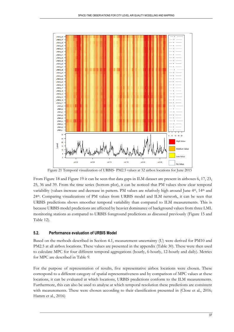
SPACE-TIME OBSERVATIONS FOR CITY LEVEL AIR QUALITY MODELLING AND MAPPING
37
Figure 21 Temporal visualization of URBIS- PM2.5 values at 32 airbox locations for June 2015
From Figure 18 and Figure 19 it can be seen that data gaps in ILM dataset are present in airboxes 6, 17, 23,
25, 36 and 39. From the time series (bottom plot), it can be noticed that PM values show clear temporal
variability (values increase and decrease in pattern. PM values are relatively high around June 4th, 14th and
24th. Comparing visualizations of PM values from URBIS model and ILM network, it can be seen that
URBIS predictions shows smoother temporal variability than compared to ILM measurements. This is
because URBIS model predictions are affected by heavier dominance of background values from three LML
monitoring stations as compared to URBIS foreground predictions as discussed previously (Figure 15 and
Table 12).
5.2. Performance evaluation of URBIS Model
Based on the methods described in Section 4.1, measurement uncertainty (U) were derived for PM10 and
PM2.5 at all airbox locations. These values are presented in the appendix (Table 30). These were then used
to calculate MPC for four different temporal aggregations (hourly, 6-hourly, 12-hourly and daily). Metrics
for MPC are described in Table 9.
For the purpose of representation of results, five representative airbox locations were chosen. These
correspond to a different category of spatial representativeness and by comparison of MPC values at these
locations, it can be evaluated at which locations, URBIS predictions conform to the ILM measurements.
Furthermore, this can also be used to analyse at which temporal resolution these predictions are consistent
with measurements. These were chosen according to their classification presented in (Close et al., 2016;
Hamm et al., 2016)

SPACE-TIME OBSERVATIONS FOR CITY LEVEL AIR QUALITY MODELLING AND MAPPING
38
Table 13 Representative airbox locations for analysis
Airbox Location Spatial Representativeness Address (Hamm et al., 2016)
1 City background Eij-erven 41, 5646 JM
31 City background (outside Eindhoven) Vincent Cleeradinlaan Waalre 5582 EJ
2 Residential area Lijmbeekstraat 190 5612 NJ
3 Busy Road Keizersgracht 28 5611GD
29 Public Hospital Ds. Fleidnerstaat 5631 BN
5.2.1. MPC results for hourly aggregation
Table 14 MPC results at five representative stations for hourly aggregations
RMSE NMB NMSD R
Spatial Representativeness
AirBox location
U RMSEu NMB MPC NMB
NMSD MPC NMSD
1-R MPC R
Hourly PM10
City Background 1 3.21 1.39 0.42 0.52 3.54 1.65 0.70 1.35
31 2.73 1.90 0.68 0.53 3.68 1.23 0.82 0.76
Residential Area 2 4.32 0.91 0.08 0.80 5.41 2.74 0.68 3.76
Busy Road 3 4.60 0.85 0.04 0.89 4.34 3.02 0.67 4.55
Public Hospital 29 4.18 0.95 0.14 0.69 3.84 2.35 0.67 2.76
Hourly PM2.5
City Background 1 1.43 1.86 0.52 0.53 2.90 1.49 0.66 1.11
31 1.37 2.08 0.60 0.54 2.86 1.29 0.82 0.83
Residential Area 2 1.74 1.38 0.26 0.69 3.73 1.98 0.61 1.96
Busy Road 3 1.94 1.20 0.16 0.72 2.94 2.11 0.61 2.23
Public Hospital 29 1.70 1.47 0.33 0.58 2.69 1.62 0.63 1.31
5.2.2. MPC results for 6-hourly aggregations
Table 15 MPC results at five representative stations for 6-hourly aggregations
Spatial Representativeness
AirBox location
U MPC RMSE
NMB MPC NMB
NMSD MPC NMSD
1-R MPC R
6-Hourly PM10
City Background 1 3.17 1.15 0.42 0.52 1.99 1.90 0.65 1.80
31 2.70 1.66 0.68 0.52 2.29 1.46 0.79 1.07
Residential Area 2 4.26 0.69 0.08 0.79 3.72 3.15 0.62 4.97
Busy Road 3 4.54 0.62 0.04 0.87 2.51 3.30 0.61 5.44
Public Hospital 29 4.13 0.70 0.14 0.68 2.23 2.70 0.58 3.66
6-Hourly PM2.5
City Background 1 1.42 1.70 0.52 0.52 3.13 1.66 0.66 1.37
31 1.36 1.91 0.60 0.53 3.79 1.43 0.83 1.02
Residential Area 2 1.72 1.22 0.26 0.68 3.24 2.15 0.59 2.32
Busy Road 3 1.92 1.05 0.16 0.71 3.12 2.23 0.59 2.49
Public Hospital 29 1.68 1.32 0.33 0.57 2.88 1.76 0.63 1.56

SPACE-TIME OBSERVATIONS FOR CITY LEVEL AIR QUALITY MODELLING AND MAPPING
39
5.2.3. MPC results for 12-hourly aggregations
Table 16 MPC results at five representative stations for 12-hourly aggregations
Spatial Representativeness
AirBox location
U MPC RMSE
NMB MPC NMB
NMSD MPC NMSD
1-R MPC R
12-Hourly PM10
City Background 1 3.15 1.09 0.42 0.51 1.79 2.16 0.65 2.33
31 2.67 1.58 0.68 0.52 2.16 1.69 0.74 1.43
Residential Area 2 4.23 0.62 0.08 0.79 3.46 3.49 0.63 6.10
Busy Road 3 4.52 0.57 0.04 0.86 1.96 3.40 0.63 5.76
Public Hospital 29 4.10 0.64 0.14 0.68 2.00 3.10 0.58 4.80
12-Hourly PM2.5
City Background 1 1.40 1.65 0.52 0.52 2.45 1.87 0.66 1.74
31 1.35 1.86 0.60 0.53 2.29 1.53 0.86 1.17
Residential Area 2 1.70 1.15 0.26 0.67 3.07 2.38 0.56 2.83
Busy Road 3 1.91 0.99 0.16 0.70 2.25 2.31 0.57 2.67
Public Hospital 29 1.66 1.26 0.33 0.57 2.22 1.96 0.61 1.93
5.2.4. MPC results for daily aggregations (24 Hour)
Table 17 MPC results at five representative stations for daily aggregations
Spatial Representativeness
AirBox location
U MPC RMSE
NMB MPC NMB
NMSD MPC NMSD
1-R MPC R
24-Hourly PM10
City Background 1 3.11 1.04 0.42 0.51 1.81 2.72 0.67 3.69
31 2.65 1.54 0.68 0.52 2.39 2.24 0.78 2.52
Residential Area 2 4.18 0.53 0.08 0.78 3.34 4.29 0.63 9.22
Busy Road 3 4.46 0.48 0.04 0.86 2.13 4.73 0.61 11.20
Public Hospital 29 4.05 0.56 0.14 0.67 2.00 3.97 0.57 7.90
24-Hourly PM2.5
City Background 1 1.38 1.52 0.52 0.51 2.08 2.37 0.76 2.80
31 1.33 1.73 0.60 0.53 1.90 1.79 1.01 1.60
Residential Area 2 1.68 1.03 0.26 0.66 2.71 2.92 0.63 4.27
Busy Road 3 1.89 0.86 0.16 0.70 1.88 2.84 0.61 4.02
Public Hospital 29 1.64 1.14 0.33 0.56 1.86 2.44 0.68 2.99
From the results, it can be seen that measurement uncertainty denoted by U (Equation 7) is lower in case
of PM2.5 as compared to PM10, owing to difference in concentration levels. There is almost no change in the
value of U for different temporal aggregations. However a contrasting feature that can be noticed is the
difference in values of U at airbox location 1 and airbox location 31 even though both are considered as city
background locations. In case of busy road (airbox location 3), the value of U is highest for both PM10 and
PM2.5 and at all temporal aggregation levels. This can be attributed to the fact that URBIS prediction values
are relatively high in busy roads. However, the heavier dominance of background values (from averaged
LML stations) may have resulted in increased values of U at all the representative airbox locations.
MPC for RMSE denoted by RMSEu (Equation 12) is generally lower for PM10 values as compared to PM2.5.
For URBIS predictions to conform with ILM measurements, RMSEu should be less than 1 The lowest
values in each case is associated with airbox located at Busy Road (Airbox location 3) and the highest values
in each case are associated with airbox location 31 and airbox location 1, which is are city background
station. MPC for RMSEu is not adhered in almost all cases of PM2.5, except for 12-hourly and daily
aggregation values at airbox location 3. RMSEu is always higher than 1 for city background station.

SPACE-TIME OBSERVATIONS FOR CITY LEVEL AIR QUALITY MODELLING AND MAPPING
40
The MPC for NMB (Equation 13) generally remained violated at city background location 31 for PM10 and
PM2.5 and remains fulfilled in all other cases. Considering the MPC for R (Equation 15), in all the cases the
MPC is fulfilled. The MPC for NMSD (Equation 14) are violated in all cases for hourly and 6-hourly
aggregations for both PM2.5 and PM10 at all airbox locations. However, for 12-hour aggregations, this is
adhered only for airbox located at busy road (for PM2.5) and for busy road and public hospital (for PM10).
In case of daily aggregations, these are only violated for city background (airbox location 31) for PM10 and
airbox location 2 (residential area) for PM2.5.
Comparison of these RMSEu values at different temporal aggregations suggest that predictions from URBIS
model were poorly consistent with ILM measurements at hourly levels and were moderately consistent at
daily values. Specifically for URBIS predictions at airbox 2, which is a spatial representative of busy roads
showed the consistent results of adhering to all MPC. whilst prediction at airbox location 1showed least
consistent results. Thus, it can be said that URBIS predictions are generally suited for locations which have
busy roads in its vicinity, and since URBIS model is an ensemble of dispersion models it is justifiable.
Furthermore, dominance of background values play a key role in the adherence of URBIS predictions to
that of ILM measurements and consequently affect MPC metrics.
5.2.5. Equal tolerance graphs (PM10) and (PM2.5)
The following plots depict the principle for equal tolerance, i.e. uncertainty levels for both model and
measurements are kept constant at 25% which is in accordance to EU Air Quality Directives (EU, 2008).
The plots depict the comparison of modelled and measured concentration levels of hourly PM10 (μg m-3)
and PM2.5 (μg m-3) for air boxes 1, 2, 3 and 31 (airbox 1 represent city background; airbox 3 represents busy
road ,airbox 2 represents residential area and airbox 31 represents city background, but is located outside
Eindhoven) those were taken as spatial representatives (Table 13). The tolerance limits of modelled and
measured concentrations are fixed at ±𝑈. These graphs are plotted at two different temporal aggregations-
daily values and hourly values for PM10 (Figure 23 and Figure 25) and PM2.5 (Figure 22 and Figure 24). Equal
tolerance graphs (Thunis et al., 2012a) infers how well model predictions overlap measurements within the
interval of measurement uncertainty. Overlap time periods are those when RMSEu values are less than 1
and model adheres to MPC for RMSE (Table 8). Analysis of these plots with RMSEu values can lead to
assessment on which temporal periods and locations, model predictions conformed to those of
measurements. The analysis of these plots are depicted in subsequent sections.
5.2.5.1. Equal tolerance graphs for hourly values
Figure 22 and Figure 23 represents the equal tolerance graphs of hourly aggregated ILM measurements and
URBIS predictions at airbox locations 1, 2, 3 and 31 for PM2.5.and PM10 respectively. It can be seen that
hourly values tend to fluctuate and these fluctuations are prominent in case of PM2.5 than that of PM10.
URBIS prediction values tend to be more than ILM measurements at all representative stations. Abrupt
increase in URBIS prediction values can be seen on dates around June 04, June 25 and on these days amongst
other, the MPC for RMSE is violated. On dates around June 07, June 19, predictions tend to overlap
measurements.
Considering airbox location 31, which is a city background station, it can be noticed that the trends in PM10
and PM2.5 values are not the same for URBIS predictions and ILM measurements, and thus has led to
increase value of RMSE violating MPCs (Table 14). Airbox locations 2 and 3 show prominent overlaps in
the URBIS predictions and ILM measurements. Airbox location 3, (busy road) in particular shows relatively
high temporal episodes of overlap and this is also seen from the MPC metrics, which is adhered to by this
location. (Table 14).

SPACE-TIME OBSERVATIONS FOR CITY LEVEL AIR QUALITY MODELLING AND MAPPING
41
5.2.5.2. Equal tolerance graphs for daily values
Figure 24 and Figure 25 represents the equal tolerance graphs of daily aggregated ILM measurements
and URBIS predictions at airbox locations 1, 2, 3 and 31 for PM2.5.and PM10 respectively. It can be seen
that there is a similar trend in URBIS prediction values at all locations. Similarly, there is also a similar
trend in ILM measurements at all locations. These trends overlap for some specific time periods, and
this overlap is greater for PM10 values than PM2.5 values. Airbox locations 2 and location 3 show
increased temporal periods of overlapping for PM10 while airbox locations 1 and 31 show fewer time
periods of overlap. Particularly for airbox location 31, least overlap is seen for PM10. In general, there is
no significant overlap of URBIS predictions and ILM measurements for PM2.5, signifying the violation
of MPC at all airbox locations except location 3 (busy road) (Table 17).
An interesting pattern can be seen from the trends of PM10 and PM2.5 at these airbox locations. For
ILM measurements, all the airbox locations have a similar temporal trend. Similarly, URBIS predictions
at all airbox locations have a similar temporal trend. This can lead to two conclusions. Firstly, URBIS
predictions as seen are high as compared to ILM measurement, Due to heavier dominance of
background concentration from averaged LML measurement stations and comparatively lower values
of URBIS foreground predictions, it can be said that there is a difference in values of ILM measurements
and that of averaged background concentration calculated from LML stations. Secondly, since ILM
measurements at all these airbox locations show similar temporal trend, mean value of ILM
measurements can be an alternative for considering background value of PM and can be used in URBIS
predictions.


SP
AC
E-T
IME
OB
SE
RV
AT
ION
S F
OR
CIT
Y L
EV
EL
AIR
QU
ALI
TY
MO
DE
LLIN
G A
ND
MA
PP
ING
43
5.2.
5.3.
H
ou
rly
agg
reg
atio
ns
Fig
ure
22 P
rin
cip
le o
f eq
ual
to
lera
nce
plo
ts f
or
ho
url
y ag
greg
atio
ns
- P
M2.5

SP
AC
E-T
IME
OB
SE
RV
AT
ION
S F
OR
CIT
Y L
EV
EL
AIR
QU
ALI
TY
MO
DE
LLIN
G A
ND
MA
PP
ING
44
Fig
ure
23 P
rin
cip
le o
f eq
ual
to
lera
nce
plo
ts f
or
ho
url
y ag
greg
atio
ns
- P
M10

SP
AC
E-T
IME
OB
SE
RV
AT
ION
S F
OR
CIT
Y L
EV
EL
AIR
QU
ALI
TY
MO
DE
LLIN
G A
ND
MA
PP
ING
45
5.2.
5.4.
D
aily
ag
gre
gat
ion
s
Fig
ure
24 P
rin
cip
le o
f eq
ual
to
lera
nce
plo
ts f
or
dai
ly a
ggre
gati
on
s -
PM
2.5

SP
AC
E-T
IME
OB
SE
RV
AT
ION
S F
OR
CIT
Y L
EV
EL
AIR
QU
ALI
TY
MO
DE
LLIN
G A
ND
MA
PP
ING
46
Fig
ure
25 P
rin
cip
le o
f eq
ual
to
lera
nce
plo
ts f
or
dai
ly a
ggre
gati
on
s -
PM
10
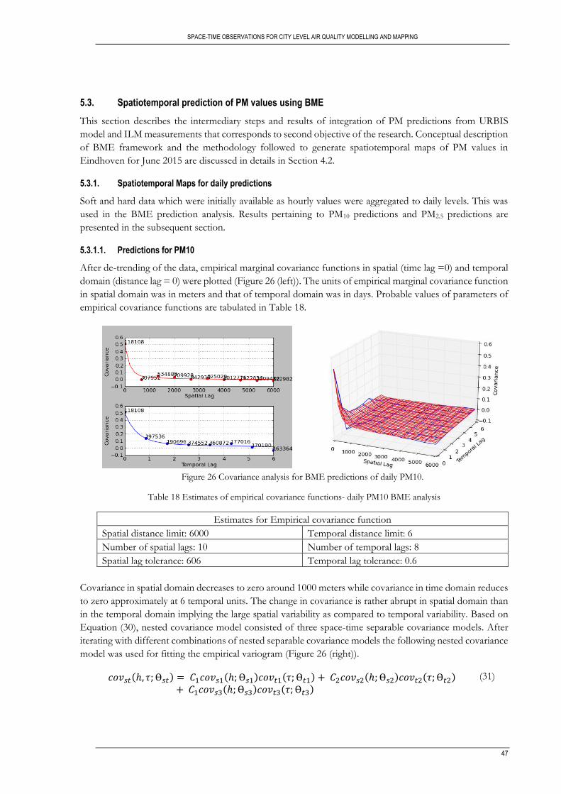
SPACE-TIME OBSERVATIONS FOR CITY LEVEL AIR QUALITY MODELLING AND MAPPING
47
5.3. Spatiotemporal prediction of PM values using BME
This section describes the intermediary steps and results of integration of PM predictions from URBIS
model and ILM measurements that corresponds to second objective of the research. Conceptual description
of BME framework and the methodology followed to generate spatiotemporal maps of PM values in
Eindhoven for June 2015 are discussed in details in Section 4.2.
5.3.1. Spatiotemporal Maps for daily predictions
Soft and hard data which were initially available as hourly values were aggregated to daily levels. This was
used in the BME prediction analysis. Results pertaining to PM10 predictions and PM2.5 predictions are
presented in the subsequent section.
5.3.1.1. Predictions for PM10
After de-trending of the data, empirical marginal covariance functions in spatial (time lag =0) and temporal
domain (distance lag = 0) were plotted (Figure 26 (left)). The units of empirical marginal covariance function
in spatial domain was in meters and that of temporal domain was in days. Probable values of parameters of
empirical covariance functions are tabulated in Table 18.
Figure 26 Covariance analysis for BME predictions of daily PM10.
Table 18 Estimates of empirical covariance functions- daily PM10 BME analysis
Estimates for Empirical covariance function
Spatial distance limit: 6000 Temporal distance limit: 6
Number of spatial lags: 10 Number of temporal lags: 8
Spatial lag tolerance: 606 Temporal lag tolerance: 0.6
Covariance in spatial domain decreases to zero around 1000 meters while covariance in time domain reduces
to zero approximately at 6 temporal units. The change in covariance is rather abrupt in spatial domain than
in the temporal domain implying the large spatial variability as compared to temporal variability. Based on
Equation (30), nested covariance model consisted of three space-time separable covariance models. After
iterating with different combinations of nested separable covariance models the following nested covariance
model was used for fitting the empirical variogram (Figure 26 (right)).
𝑐𝑜𝑣𝑠𝑡(ℎ, 𝜏; Ɵ𝑠𝑡) = 𝐶1𝑐𝑜𝑣𝑠1(ℎ; Ɵ𝑠1)𝑐𝑜𝑣𝑡1(𝜏; Ɵ𝑡1) + 𝐶2𝑐𝑜𝑣𝑠2(ℎ; Ɵ𝑠2)𝑐𝑜𝑣𝑡2(𝜏; Ɵ𝑡2) + 𝐶1𝑐𝑜𝑣𝑠3(ℎ; Ɵ𝑠3)𝑐𝑜𝑣𝑡3(𝜏; Ɵ𝑡3)
(31)
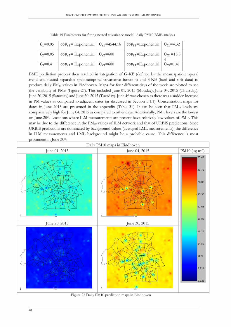
SPACE-TIME OBSERVATIONS FOR CITY LEVEL AIR QUALITY MODELLING AND MAPPING
48
Table 19 Parameters for fitting nested covariance model- daily PM10 BME analysis
𝐶1=0.05 𝑐𝑜𝑣𝑠1= Exponential Ɵ𝑠1=4544.16 𝑐𝑜𝑣𝑡1=Exponential Ɵ𝑡1=4.32
𝐶2=0.05 𝑐𝑜𝑣𝑠2= Exponential Ɵ𝑠2=600 𝑐𝑜𝑣𝑡2=Exponential Ɵ𝑡2 =18.8
4 𝐶3=0.4 𝑐𝑜𝑣𝑠3= Exponential Ɵ𝑠3=600 𝑐𝑜𝑣𝑡3=Exponential Ɵ𝑡3=1.41
BME prediction process then resulted in integration of G-KB (defined by the mean spatiotemporal
trend and nested separable spatiotemporal covariance function) and S-KB (hard and soft data) to
produce daily PM10 values in Eindhoven. Maps for four different days of the week are plotted to see
the variability of PM10 (Figure 27). This included June 01, 2015 (Monday), June 04, 2015 (Thursday),
June 20, 2015 (Saturday) and June 30, 2015 (Tuesday). June 4th was chosen as there was a sudden increase
in PM values as compared to adjacent dates (as discussed in Section 5.1.1). Concentration maps for
dates in June 2015 are presented in the appendix (Table 31). It can be seen that PM10 levels are
comparatively high for June 04, 2015 as compared to other days. Additionally, PM10 levels are the lowest
on June 20th. Locations where ILM measurements are present have relatively low values of PM10. This
may be due to the difference in the PM10 values of ILM network and that of URBIS predictions. Since
URBIS predictions are dominated by background values (averaged LML measurements), the difference
in ILM measurements and LML background might be a probable cause. This difference is most
prominent in June 30th.
Daily PM10 maps in Eindhoven
June 01, 2015 June 04, 2015 PM10 (μg m-3)
June 20, 2015 June 30, 2015
Figure 27 Daily PM10 prediction maps in Eindhoven

SPACE-TIME OBSERVATIONS FOR CITY LEVEL AIR QUALITY MODELLING AND MAPPING
49
5.3.1.2. Predictions for PM2.5
Similarly, BME analysis to generate spatiotemporal maps for daily values of PM2.5 were carried out. The
empirical covariance functions in space and time domain were generated (Table 20) and by means of nested
space-time separable covariance function (Equation 30), model fitting was done. Figure 28 represents the
empirical covariance functions in space and time (left) and the fitted covariance model (right). The units for
spatial lag is meters and temporal lag is days. It can be noticed that the effective range for the covariance in
spatial domain is approximately 4000 meters whilst that for temporal domain is approximately 6 days. It can
be noticed that the slope of both spatial and temporal covariance functions are smooth and give an
indication that there is no sudden change in spatiotemporal variability.
Figure 28 Covariance analysis for BME predictions of daily PM2.5
Table 20 Estimates of empirical covariance functions- daily PM2.5 BME analysis
Estimates for Empirical covariance function
Spatial distance limit: 4000 Temporal distance limit: 6
Number of spatial lags: 10 Number of temporal lags: 8
Spatial lag tolerance: 450 Temporal lag tolerance: 0.8
The modelled space-time covariance function consisted of three space time separable covariance functions
and its parameters are depicted in Table 21. This was used to generate spatiotemporal maps of PM2.5 for
daily values.
Table 21 Parameters for fitting nested covariance model- daily PM2.5 BME analysis
𝐶1=0.05 𝑐𝑜𝑣𝑠1= Exponential Ɵ𝑠1=5509.58 𝑐𝑜𝑣𝑡1=Exponential Ɵ𝑡1=2.28
𝐶2=0.15 𝑐𝑜𝑣𝑠2= Exponential Ɵ𝑠2=975.63 𝑐𝑜𝑣𝑡2=Exponential Ɵ𝑡2=2.7
𝐶3=0.1 𝑐𝑜𝑣𝑠3= Exponential Ɵ𝑠3=943.42 𝑐𝑜𝑣𝑡3=Exponential Ɵ𝑡3=0.6
𝑐𝑜𝑣𝑠𝑡(ℎ, 𝜏; Ɵ𝑠𝑡) = 𝐶1𝑐𝑜𝑣𝑠1(ℎ; Ɵ𝑠1)𝑐𝑜𝑣𝑡1(𝜏; Ɵ𝑡1) + 𝐶2𝑐𝑜𝑣𝑠2(ℎ; Ɵ𝑠2)𝑐𝑜𝑣𝑡2(𝜏; Ɵ𝑡2) + 𝐶1𝑐𝑜𝑣𝑠3(ℎ; Ɵ𝑠3)𝑐𝑜𝑣𝑡3(𝜏; Ɵ𝑡3)
(32)

SPACE-TIME OBSERVATIONS FOR CITY LEVEL AIR QUALITY MODELLING AND MAPPING
50
PM2.5 prediction maps are shown for four days of June 2015 (Figure 29). Concentration maps for dates in
June 2015 are presented in the appendix (Table 32). The pattern corresponds in a similar manner to that of
PM10 predictions (Figure 27). PM2.5 values tend to be high on June 04 and lowest for June 20. There is a
decrease in PM2.5 level at locations near to ILM measurements and can be asserted to difference in URBIS
predictions and ILM measurements.
Daily PM2.5 maps in Eindhoven
June 01, 2015 June 04, 2015 PM2.5 (μg m-3)
June 20, 2015 June 30, 2015
Figure 29 Daily PM2.5 prediction maps in Eindhoven
5.3.1.3. Cross validation
Cross validation of BME predictions were assessed by means of leave-one-out method employed in STAR-
BME. 2000 soft and hard data were chosen in random and predictions were obtained at those locations.
RMSE value was low for PM2.5 predictions as compared to PM10. It might be due to the fact the spatial
variability is high in PM10 as compared to PM2.5 (as seen from the empirical covariance function for spatial
domain (Figure 26, Figure 28). Table 22 Cross validation results- daily predictions BME
BME
Prediction
Data RMSE Residual
Mean
Residual Standard
Deviation
PM10 Daily 200 soft and
hard
1.48 0.24 1.46
PM2.5 Daily 2000 soft and
hard
0.85 0.05 0.85

SPACE-TIME OBSERVATIONS FOR CITY LEVEL AIR QUALITY MODELLING AND MAPPING
51
5.3.2. Spatiotemporal Maps for hourly predictions
To understand about spatiotemporal variability of PM in a day, hourly prediction maps were generated.
These were done for June 04, 2015, which showed an abrupt increase in PM values (as discussed in Section
5.1.1). Hourly soft and hard data pertaining to June 4th were used in the BME analysis. Spatiotemporal maps
of hourly values of PM10 predictions and PM2.5 predictions are presented in the subsequent section.
5.3.2.1. Predictions for PM10
Empirical space-time covariance functions were estimated from the given data (Table 23). Marginal
covariance functions in space and time domain were plotted in Figure 30 Covariance analysis for BME
predictions of hourly PM The unit for spatial lag is in meters and that for temporal lag is in hour. From the
empirical covariance functions, it can be seen that the covariance value is relatively high as compared to
daily values (Figure 26). There us a smooth decrease in the spatial and temporal covariance of PM10 values.
Figure 30 Covariance analysis for BME predictions of hourly PM10
Table 23 Estimates of empirical covariance functions- hourly PM10 BME analysis
Estimates for Empirical covariance function
Spatial distance limit: 4000 Temporal distance limit: 8.
Number of spatial lags: 8 Number of temporal lags: 8
Spatial lag tolerance: 800 Temporal lag tolerance: 0.6
The modelled space-time covariance function consisted of three space time separable covariance functions
and its parameters are depicted in Table 23. This was used to generate spatiotemporal maps of PM10 for
hourly values.
Table 24 Parameters for fitting nested covariance model– hourly PM10 BME analysis
𝐶1=0.65 𝑐𝑜𝑣𝑠1= Exponential Ɵ𝑠1=953.85 𝑐𝑜𝑣𝑡1=Gaussian Ɵ𝑡1=1.1
𝐶2=0.38 𝑐𝑜𝑣𝑠2= Exponential Ɵ𝑠2=5444.88 𝑐𝑜𝑣𝑡2= Gaussian Ɵ𝑡2=8.38
𝐶3=0.36 𝑐𝑜𝑣𝑠3= Exponential Ɵ𝑠3=4599.87 𝑐𝑜𝑣𝑡3= Gaussian Ɵ𝑡3=0.8
𝑐𝑜𝑣𝑠𝑡(ℎ, 𝜏; Ɵ𝑠𝑡) = 𝐶1𝑐𝑜𝑣𝑠1(ℎ; Ɵ𝑠1)𝑐𝑜𝑣𝑡1(𝜏; Ɵ𝑡1) + 𝐶2𝑐𝑜𝑣𝑠2(ℎ; Ɵ𝑠2)𝑐𝑜𝑣𝑡2(𝜏; Ɵ𝑡2) + 𝐶1𝑐𝑜𝑣𝑠3(ℎ; Ɵ𝑠3)𝑐𝑜𝑣𝑡3(𝜏; Ɵ𝑡3)
(33)

SPACE-TIME OBSERVATIONS FOR CITY LEVEL AIR QUALITY MODELLING AND MAPPING
52
In June 04, 2015, four time periods were chosen at 6 hour intervals for representation purposes.
Concentration maps for all hourly time periods in June 04 2015 are presented in the appendix (Table 33).
These were 03:00 to 04:00, 09:00 to 10:00, 15:00 to 16:00 and 21:00-22:00 hours and corresponded to late
night, post- morning rush hour, afternoon rush hours and before midnight. PM10 values tends to gradually
increase through the day till afternoon rush hour after which it tends to recede. However, these values
(21:00-22:00 hours) tend to remain high as compared to morning rush hour. Regions around ILM
measurement stations have lower value of PM10 as compared to other locations and is prominent at all the
cases.
Hourly PM10 maps in Eindhoven
03:00 to 04:00 hours 09:00-10:00 hours PM10 (μg m-3)
15:00-16:00 hours 21:00-22:00 hours
Figure 31 Hourly PM10 prediction maps in Eindhoven
5.3.2.2. Predictions for PM2.5
BME analysis using hourly PM2.5 values of ILM measurement and URBIS predictions for June 04, 2015
were done to generate hourly spatiotemporal maps. The empirical covariance functions in spatial and
temporal domains are plotted (Figure 32) using estimates from the data (Table 25). The unit of empirical
covariance functions in spatial domain is meters and temporal domain is hour. The spatial covariance
function has an effective range of 4000 meters, beyond which it is considered that there is no correlation
among the values. Similarly, the temporal covariance function has an effective range of approximately 6
days. The decrease in covariance values are gradual in case of temporal covariance function while spatial
covariance decreases abruptly up to 1000 meters.

SPACE-TIME OBSERVATIONS FOR CITY LEVEL AIR QUALITY MODELLING AND MAPPING
53
Figure 32 Covariance analysis for BME predictions of hourly PM2.5
Table 25 Estimates of empirical covariance functions- hourly PM2.5 BME analysis
Estimates for Empirical covariance function
Spatial distance limit: 4000 Temporal distance limit: 6
Number of spatial lags: 10 Number of temporal lags: 8
Spatial lag tolerance: 500 Temporal lag tolerance: 0.5
The modelled space-time covariance function consisted of three space time separable covariance functions
and its parameters are depicted in (Table 26). This was used to generate spatiotemporal maps of PM2.5 for
hourly values on June 04, 2015.
Table 26 Parameters for fitting nested covariance model- hourly PM2.5 BME analysis
𝐶1=0.36 𝑐𝑜𝑣𝑠1= Exponential Ɵ𝑠1=662.63 𝑐𝑜𝑣𝑡1=Exponential Ɵ𝑡1=7.85
𝐶2=0.05 𝑐𝑜𝑣𝑠2= Exponential Ɵ𝑠2=7132.61 𝑐𝑜𝑣𝑡2=Exponential Ɵ𝑡2=12.39
𝐶3=0.06 𝑐𝑜𝑣𝑠3= Exponential Ɵ𝑠3=7411.57 𝑐𝑜𝑣𝑡3=Exponential Ɵ𝑡3=15.36
Similar to hourly PM10 analysis, four time periods were chosen each at six hour intervals to see the
spatiotemporal variability of PM2.5 values in Eindhoven (Figure 33). Concentration maps for all hourly time
periods in June 04 2015 are presented in the appendix (Table 34). The values tend to be low during late
night (03:00-04:00) hours and increase through the day. PM2.5 concentrations are the highest during 21:00-
22:00 hours. Unlike hourly PM10 predictions (Figure 31) which showed highest concentration levels during
afternoon rush hour (15:00-16:00) hours and then stabilizes, PM2.5 shows an increasing trend in values.
Furthermore, locations around ILM measurements have lower concentration that other regions, but in
comparison with hourly PM10 predictions (Figure 31), these changes are not so prominent.
𝑐𝑜𝑣𝑠𝑡(ℎ, 𝜏; Ɵ𝑠𝑡) = 𝐶1𝑐𝑜𝑣𝑠1(ℎ; Ɵ𝑠1)𝑐𝑜𝑣𝑡1(𝜏; Ɵ𝑡1) + 𝐶2𝑐𝑜𝑣𝑠2(ℎ; Ɵ𝑠2)𝑐𝑜𝑣𝑡2(𝜏; Ɵ𝑡2) + 𝐶1𝑐𝑜𝑣𝑠3(ℎ; Ɵ𝑠3)𝑐𝑜𝑣𝑡3(𝜏; Ɵ𝑡3)
(34)

SPACE-TIME OBSERVATIONS FOR CITY LEVEL AIR QUALITY MODELLING AND MAPPING
54
Hourly PM2.5 maps in Eindhoven
03:00 to 04:00 hours 09:00-10:00 hours PM2.5 (μg m-3)
15:00-16:00 hours 21:00-22:00 hours
Figure 33 Hourly PM2.5 prediction maps in Eindhoven
5.3.2.3. Cross Validation
To assess the prediction accuracy of BME process, leave-one-out cross validation was carried out taking
into consideration 2000 soft and hard data locations (Table 27).PM2.5 predictions had a lower RMSE and
residual mean as compared to PM10 predictions. PM10 hourly predictions had extremely high value of RMSE
and residual standard deviation.
Table 27 Cross validation results- hourly predictions BME
BME analysis Data RMSE Residual Mean Residual
Standard
Deviation
PM2.5 Hourly 2000 soft and
hard
0.95 0.13 0.94
PM10 Hourly 2000 soft data 3.475 0.57 3.42

SPACE-TIME OBSERVATIONS FOR CITY LEVEL AIR QUALITY MODELLING AND MAPPING
55
5.4. Comparison of mean ILM measurements with averaged LML for background PM
As discussed in Section 5.1, relatively lower value of ILM mean measurements against that of LML
background values (Table 12 and Figure 15) and no discernible differences in the mean PM values across
the categorizes of airbox locations (Figure 16 and Figure 17) can suggest that mean values of ILM can also
be assumed as the background value of PM in Eindhoven. Timeseries plot (Figure 34) shows that mean
ILM PM2.5 values at a daily level tend to remain between 5- 10 μg m-3 and show less fluctuations as
compared to averaged background from LML stations
Figure 34 Timeseries of mean ILM values and averaged background from LML stations
To compare the effect of PM background values on performance of URBIS predictions and on BME
analysis, one special case was considered. Mean PM2.5 ILM measurements were used as background values
for URBIS background predictions instead of averaged PM2.5 LML measurements. This was done for daily
values of PM2.5 and the results were compared with corresponding results obtained by taking averaged LML
measurements as background value (Section 5.3.1.2 and Section 5.2.5).
5.4.1.1. Spatiotemporal predictions of daily PM2.5 using mean ILM as background
Aggregated daily values of PM2.5 URBIS foreground predictions were added to averaged ILM measurements
(PM2.5) at 32 airbox locations to obtain new URBIS predictions at 500 locations. Uncertainty in these URBIS
predictions was kept constant at 25%, that corresponded to maximum allowable uncertainty in daily PM2.5
measurements as set by air quality guidelines (EU, 2008). Soft data at these locations was thus generated by
using the bounds of ± 25% of the URBIS prediction values. Hard data comprised of daily aggregated PM2.5
ILM measurements at 32 locations.
BME was then performed to generate spatiotemporal predictions of daily PM2.5 values in Eindhoven. The
empirical covariance function in spatial domain and temporal domain were estimated from the data (Figure
35 and Table 28). A high value of spatial covariance is seen for 3000 meters while the temporal covariance
reduces to zero approximately at 1 day lag. The units of spatial lag is meters and that of temporal lag is days.

SPACE-TIME OBSERVATIONS FOR CITY LEVEL AIR QUALITY MODELLING AND MAPPING
56
Figure 35 Covariance analysis for BME predictions of daily PM2.5 (using ILM as background)
Table 28 Estimates of empirical covariance functions- Daily PM2.5 BME analysis (using ILM as background)
Estimates for Empirical covariance function
Spatial distance limit: 3000 Temporal distance limit: 8
Number of spatial lags: 10 Number of temporal lags: 8
Spatial lag tolerance: 200 Temporal lag tolerance: 0.7
The modelled space-time covariance function consisted of three space time separable covariance functions
and its parameters are depicted in Table 29. This was used to generate spatiotemporal maps of PM2.5 for
daily values.
Table 29 Parameters for fitting nested covariance model– Daily PM2.5 BME analysis (using ILM as background)
𝐶1=0.28 𝑐𝑜𝑣𝑠1= Gaussian Ɵ𝑠1=300 𝑐𝑜𝑣𝑡1=Spherical Ɵ𝑡1=1.11
𝐶2=1.17 𝑐𝑜𝑣𝑠2= Gaussian Ɵ𝑠2=15000 𝑐𝑜𝑣𝑡2=Spherical Ɵ𝑡2=0.87
𝐶3=0.13 𝑐𝑜𝑣𝑠3= Gaussian Ɵ𝑠3=300 𝑐𝑜𝑣𝑡3=Spherical Ɵ𝑡3=0.8
Spatiotemporal prediction maps for daily PM2.5 values in Eindhoven were plotted for four dates (June 01,
June 04, June 20 and June 30, 2015). These dates were chosen for comparison with daily PM2.5 BME
predictions that was previously done using LML measurements as background stations for URBIS
predictions (Section 5.3.1.2). From the plots (Figure 36) it can be seen that PM2.5 values are comparatively
high for June 04 and lowest for June 20. One striking feature that can be noticed while comparing these
plots with corresponding plots in Figure 29, is that, there is no such distinguishable difference in PM2.5
values around the airbox locations (shown as dots). This is in contrast with observations from Figure 29,
where differences in PM2.5 values around airbox locations were prominent and can suggests that fluctuations
in these values were mainly due to averaged LML measurements used as background concentrations.
𝑐𝑜𝑣𝑠𝑡(ℎ, 𝜏; Ɵ𝑠𝑡) = 𝐶1𝑐𝑜𝑣𝑠1(ℎ; Ɵ𝑠1)𝑐𝑜𝑣𝑡1(𝜏; Ɵ𝑡1) + 𝐶2𝑐𝑜𝑣𝑠2(ℎ; Ɵ𝑠2)𝑐𝑜𝑣𝑡2(𝜏; Ɵ𝑡2) + 𝐶1𝑐𝑜𝑣𝑠3(ℎ; Ɵ𝑠3)𝑐𝑜𝑣𝑡3(𝜏; Ɵ𝑡3)
(35)

SPACE-TIME OBSERVATIONS FOR CITY LEVEL AIR QUALITY MODELLING AND MAPPING
57
Daily PM2.5 maps in Eindhoven (Using mean ILM values as background)
June 01, 2015 June 04, 2015 PM2.5 (μg m-3)
June 25, 2015 June 30, 2015
Figure 36 Daily PM2.5 prediction maps in Eindhoven (using ILM as background)
Cross validation of the BME process was done using leave-one out method in the similar manner as
described in Section 5.3.1.3 and it was found that RMSE associated with the prediction was 0.89, the residual
mean was 0.16 and residual standard deviation was 0.87. This was found to be comparable with cross
validation results of BME predictions where averaged LML measurements were used as background values,
which had RMSE of 0.85, the residual mean as 0.05 and residual standard deviation as 0.85.
Equal tolerance graphs, described in Section 5.2.5 were plotted to assess the conformance of daily PM2.5
values of URBIS predictions against daily PM2.5 values of ILM measurements. Here uncertainty levels for
both URBIS model predictions and ILM measurements are kept constant at 25%. These were plotted for
four different locations (Figure 37)- airbox location 1 (City background), airbox location 2 (Busy road),
airbox location 3 (Residential area) and airbox location 31 (City background –outside Eindhoven). These
plots show that there is a high conformance in URBIS predictions and ILM measurements. Particularly at
airbox location 2, URBIS predictions and ILM measurements are almost identical for all dates of June 2015.
For airbox location 3, which corresponds to busy road, URBIS predictions are higher than that of ILM
measurements and this can be attributed to URBIS foreground values. Thus it can be asserted that mean
values of ILM measurements can be used as background values for PM2.5 in Eindhoven and facilitate
integration of URBIS predictions with ILM measurements.

SP
AC
E-T
IME
OB
SE
RV
AT
ION
S F
OR
CIT
Y L
EV
EL
AIR
QU
ALI
TY
MO
DE
LLIN
G A
ND
MA
PP
ING
58
Fig
ure
37 P
rin
cip
le o
f eq
ual
to
lera
nce
- d
aily
agg
rega
ted
PM
2.5
(usi
ng
ILM
as
bac
kgr
oun
d in
UR
BIS
pre
dic
tio
ns)

SPACE-TIME OBSERVATIONS FOR CITY LEVEL AIR QUALITY MODELLING AND MAPPING
59
6. DISCUSSION
This chapter discusses of some of the key findings of the research. It includes discussions in particular about
the data quality of URBIS predictions and ILM measurements, estimation of background PM values, levels
of uncertainty in PM measurements, interpretation of performance evaluation results and feasibility of BME
method in integration of URBIS and ILM.
6.1.1. Data quality of URBIS and ILM
ILM dataset contained missing measurements for a prolonged time periods at some airboxes (Table 3; Figure
18 and Figure 19) due to which evaluation of URBIS predictions at these time points was not possible. MPC
values were calculated for only those time points at which ILM measurements and URBIS predictions were
both available. Reduction in these modelled-concentration pairs thus influenced MPC results at those airbox
locations. URBIS dataset only consisted of foreground predictions of PM which were mainly traffic
contributions from highways and streets canyons (Table 4). It lacked contributions from emissions by point
and area sources, such as industries, building construction sites, agricultural land which amongst other have
substantial impact on PM values in a city. Thus it was deemed necessary to account for background PM
values for adequate representation of URBIS predictions prior evaluating them against ILM measurements.
6.1.2. Estimation of background values of PM
To account for contribution of background levels in the PM values in Eindhoven, measurements from three
LML stations were averaged and its mean value was considered. These stations were classified as background
stations and were located in vicinity of Eindhoven (Section 3.2.3.2). By analysing the PM values at these
stations (Figure 8, Figure 9 and Figure 10), it was noticed that average value can be the approximation of
values at these three stations. This was also confirmed from Table 7 where averaged background showed
almost similar values with individual LML stations. Averaged PM values from LML stations were high as
compared to the URBIS foreground predictions. This is described in Section 5.1 (Table 12 and Figure 15).
Low values of URBIS foreground predictions as compared to ILM measurements and averaged LML
background were in accordance with Matthijsen & ten Brink, (2007) suggesting low contribution of local
traffic sources to PM2.5 values in the Netherlands. Heavier dominance of this background concentration in
URBIS predictions can also be seen in the temporal visualization of URBIS predictions at airbox locations
(Figure 20 and Figure 21).
From Table 12 and Figure 15, it can also be noticed that the averaged LML measurements (mean value)
were also larger than mean of ILM measurements. It might lead to the following conclusions. Firstly,
averaging measurements from these three available LML stations might not be adequate representation of
background values in Eindhoven. Furthermore, abrupt hourly fluctuations in PM measurements at any
individual LML station (Figure 9,Figure 10), missing values, discarding of negative values (Section 3.2.3.2)
while averaging can lead to a biased estimation of average. Secondly, ILM instruments might record lower
values of PM as compared to LML stations. Recent analysis performed by the AiREAS
Calibration/Validation working group has shown that the ILM instruments often record lower values of
PM relative to LML station located at Genovevalaan, Eindhoven (Otjes, 2016). It is early to say how
widespread the problem is. However, it may explain why the background values recorded by the LML
stations located outside Eindhoven contribute to URBIS predictions that are often larger than spatially
coincident ILM measurements. Thirdly, relatively lower value of mean ILM measurements against averaged

SPACE-TIME OBSERVATIONS FOR CITY LEVEL AIR QUALITY MODELLING AND MAPPING
60
LML background stations as discussed above and similarity in PM levels for different categorizes of airboxes
(Figure 16 and Figure 17) might lead to the fact that mean ILM measurements can also be used as
background values in place of averaged LML measurements in the URBIS model. Mean ILM measurements
also showed less fluctuations in their values as compared to averaged LML measurements (Figure 34).
6.1.3. Uncertainty levels in PM values
Uncertainty associated with measurements of PM values were assumed to be 25% of their values for ILM
network at all temporal scales of aggregation (Section 4.1) due to inadequate information on its exact value.
This was based on relative uncertainty of 25% in mean PM measurements (PM10 and PM2.5) which is a
reference value that stems from the European air quality directive and is considered for daily values (EU,
2008). It is because PM values tend to fluctuate and other systematic and random errors associated with
measurements which makes it difficult to impose a reference value of uncertainty for lower temporal scales.
Changing the temporal scale to hourly or 6-hourly or 24-hourly may result in the increase of uncertainty but
the exact value could not be ascertained.
To elucidate principle of equal tolerance which assumes model to exhibit similar levels in uncertainty in PM
values as compared to measurements, URBIS model predictions were also assumed to have 25 % uncertainty
in their values. This assumption is justifiable owing to that fact that major contribution in URBIS prediction
was from the background values which were from the LML stations. These measurements have 16%
uncertainty associated with them and is explained in Section 3.2.3.2 and also established by reports of
(Hoogerbrugge et al., 2010). Assumption of averaged LML measurements as background value also
incorporate additional uncertainties in the PM values of URBIS. Inherent uncertainties associated in the
dispersion modelling frameworks employed in the URBIS also account for additional uncertainties.
Possibility of performing a sensitivity analysis on URBIS model could have led to discerning these
uncertainties but outside the scope of the research. Thus, based on these factors led to the assumption of
uncertainty of 25% in URBIS data. This value was kept constant for all temporal scales (hourly and daily
level) for the analysis due to lack of information about exact levels of uncertainty of PM predictions in
URBIS at these temporal aggregations.
6.1.4. Performance evaluation of URBIS model
Measurement uncertainty were calculated for each airbox, taking into consideration relative uncertainty of
25% for measurement of PM values as set by air quality directives. These values were found to be high for
PM10 and lower for PM2.5 values at all temporal scales of aggregation. From Section 5.2 , it can be seen that
aggregation of ILM measurements and URBIS predictions from hourly to 24-hourly resulted in almost no
change in measurement uncertainty values. This might be due to the fact that aggregation tends to smooth
out variations and the mean value of observations remains approximately the same. Furthermore,
assumption of 25% relative measurement uncertainty for PM values at all temporal scales might have
resulted in no change in measurement uncertainty at these airboxes. Model performance criteria for RMSE
was found to be consistently violated at all representative airbox locations for PM2.5 at all temporal
aggregations, except in case of busy road (for 12-hourly and daily aggregations). The MPC for RMSE and
NMB was violated only in city background locations for PM10. MPC for RMSE values remains low at
locations which represent busy roads, owing to fact that URBIS predictions are generally better for locations
near to traffic sources and these values were high for regions such as city background which have fewer
traffic. Model performance criteria for R remains fulfilled at all locations whilst MPC for NMSD remains
violated for all locations in hourly and 6-hourly aggregations. For 12 hourly and daily aggregations, these are
only violated in city background (PM10) and only adhered in busy road locations.
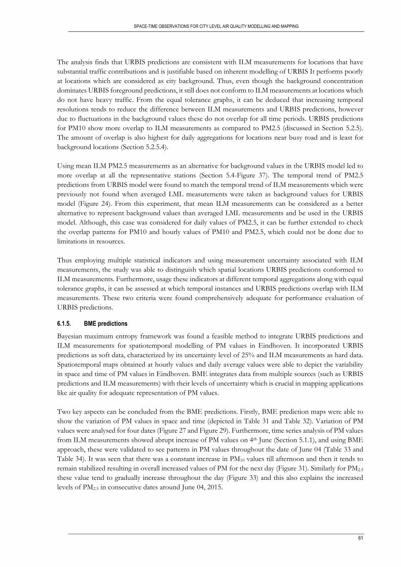
SPACE-TIME OBSERVATIONS FOR CITY LEVEL AIR QUALITY MODELLING AND MAPPING
61
The analysis finds that URBIS predictions are consistent with ILM measurements for locations that have
substantial traffic contributions and is justifiable based on inherent modelling of URBIS It performs poorly
at locations which are considered as city background. Thus, even though the background concentration
dominates URBIS foreground predictions, it still does not conform to ILM measurements at locations which
do not have heavy traffic. From the equal tolerance graphs, it can be deduced that increasing temporal
resolutions tends to reduce the difference between ILM measurements and URBIS predictions, however
due to fluctuations in the background values these do not overlap for all time periods. URBIS predictions
for PM10 show more overlap to ILM measurements as compared to PM2.5 (discussed in Section 5.2.5).
The amount of overlap is also highest for daily aggregations for locations near busy road and is least for
background locations (Section 5.2.5.4).
Using mean ILM PM2.5 measurements as an alternative for background values in the URBIS model led to
more overlap at all the representative stations (Section 5.4-Figure 37). The temporal trend of PM2.5
predictions from URBIS model were found to match the temporal trend of ILM measurements which were
previously not found when averaged LML measurements were taken as background values for URBIS
model (Figure 24). From this experiment, that mean ILM measurements can be considered as a better
alternative to represent background values than averaged LML measurements and be used in the URBIS
model. Although, this case was considered for daily values of PM2.5, it can be further extended to check
the overlap patterns for PM10 and hourly values of PM10 and PM2.5, which could not be done due to
limitations in resources.
Thus employing multiple statistical indicators and using measurement uncertainty associated with ILM
measurements, the study was able to distinguish which spatial locations URBIS predictions conformed to
ILM measurements. Furthermore, usage these indicators at different temporal aggregations along with equal
tolerance graphs, it can be assessed at which temporal instances and URBIS predictions overlap with ILM
measurements. These two criteria were found comprehensively adequate for performance evaluation of
URBIS predictions.
6.1.5. BME predictions
Bayesian maximum entropy framework was found a feasible method to integrate URBIS predictions and
ILM measurements for spatiotemporal modelling of PM values in Eindhoven. It incorporated URBIS
predictions as soft data, characterized by its uncertainty level of 25% and ILM measurements as hard data.
Spatiotemporal maps obtained at hourly values and daily average values were able to depict the variability
in space and time of PM values in Eindhoven. BME integrates data from multiple sources (such as URBIS
predictions and ILM measurements) with their levels of uncertainty which is crucial in mapping applications
like air quality for adequate representation of PM values.
Two key aspects can be concluded from the BME predictions. Firstly, BME prediction maps were able to
show the variation of PM values in space and time (depicted in Table 31 and Table 32). Variation of PM
values were analysed for four dates (Figure 27 and Figure 29). Furthermore, time series analysis of PM values
from ILM measurements showed abrupt increase of PM values on 4th June (Section 5.1.1), and using BME
approach, these were validated to see patterns in PM values throughout the date of June 04 (Table 33 and
Table 34). It was seen that there was a constant increase in PM10 values till afternoon and then it tends to
remain stabilized resulting in overall increased values of PM for the next day (Figure 31). Similarly for PM2.5
these value tend to gradually increase throughout the day (Figure 33) and this also explains the increased
levels of PM2.5 in consecutive dates around June 04, 2015.

SPACE-TIME OBSERVATIONS FOR CITY LEVEL AIR QUALITY MODELLING AND MAPPING
62
Secondly, BME was able to discern the local variability in PM values at regions near airboxes. This variation
in PM values were prominent for both PM10 and PM2.5 at hourly and daily scales (Section 5.3). This is due
to high values of URBIS predictions as compared to ILM measurements. These high values of URBIS
predictions, as discussed in Section 6.1.2 is primarily due to averaged LML measurements that was
considered as background values for URBIS model. This change in values is most prominent in hourly PM10
predictions (Figure 31). Another possible reason behind this variability can be the use of kernel smoothing
filter that is employed in STAR-BME to remove spatiotemporal mean trend. Modification of values for this
kernel smoothing filter might have led to a low differences in PM values in the adjacent regions of airboxes.
However, this modification was not possible currently and can be considered in future. The cross validation
results for BME were seen to acceptable for PM2.5 (RMSE of 0.85 for daily predictions and 0.95 for hourly
predictions but these RMSE values were comparatively high for PM10 predictions (Table 22 and Table 27).
Specifically for hourly PM10 RMSE value was 3.7 which might raise a question on BME’s effectiveness for
PM10 modelling. This can be addressed by comparing BME predictions with those obtained by other
interpolation methods (such as regression kriging) and can be considered as future scope.
In order to assess the effect of background value on BME predictions, mean ILM measurements were taken
as background for URBIS predictions (Section 5.4) and used for daily predictions of PM2.5. From the
results, (Figure 36), it can be seen that there were relatively less variations in PM2.5 values near airbox
locations, as compared to the predictions where averaged LML measurements were taken as background
values for URBIS (Figure 29). This further ascertains that mean ILM measurements can be used as an
alternative to averaged LML measurements as background levels of PM2.5 in Eindhoven. The cross
validation results for the case where mean ILM measurements were taken as background value was found
to be comparable with daily PM2.5 predictions (RMSE value of 0.89). Although this was only one
experimental case which was considered (for daily values of PM2.5 predictions), it could be further extended
for daily PM10 predictions and hourly predictions. Based on these results, it can be concluded that ILM
measurements can be incorporated with URBIS model predictions for spatiotemporal modelling and
mapping of PM values in Eindhoven.

SPACE-TIME OBSERVATIONS FOR CITY LEVEL AIR QUALITY MODELLING AND MAPPING
63
7. CONCLUSIONS
Based on research identification outlined in Section 1.3, this research comprised firstly of evaluation of PM
predictions (PM10 and PM2.5) from the downscaled URBIS against PM measurements (PM10 and PM2.5)
from the ILM to assess at which temporal resolution URBIS predictions resembled ILM measurements.
This was done by means of statistical metrics utilizing uncertainty levels associated with PM measurements
in the ILM. Conceptual description of the methodologies for performance evaluation have been outlined in
Section 4.1.1. Four recommended statistical metrics for air quality evaluation, namely, root mean square
error (RMSE), normalized mean bias (NMB), normalized mean standard deviation (NMSD) and correlation
co-efficient (R) were used with measurement uncertainty of PM (assumed to be 25% of the measured PM
values), lead to formulation of model performance criteria (MPC). Assessment of URBIS predictions against
ILM was carried out at 32 ILM measurement locations and at four different temporal scales were done at
four different temporal scales- hourly, 6-hourly, 12-hourly and daily values for June 2015. These results are
described in Section 5.2.
Secondly, this study employed BME method to integrate URBIS predictions with ILM measurements for
spatiotemporal mapping of PM values (PM10 and PM2.5) in Eindhoven. PM values from 500 URBIS
prediction locations and 32 ILM locations for June 2015 were used for BME mapping. Predictions were
done at two temporal scales - aggregated daily values (entire month of June, 2015) and hourly values (for
June 4th, 2015). Conceptual description of BME method is described in Section 4.2.1. Intermediary process
and spatiotemporal maps at these temporal scales are depicted in Section 5.3.
7.1. Answer to research questions
Questions related to objective 1:
a) What are the key statistical indicators that are needed to evaluate URBIS model?
After an extensive literature review focussing on evaluating air quality models (Section 2.3) and based
on conceptual description (Section 4.1.1), it was found that application of multiple statistical indicators
are required for evaluating URBIS model. These were root mean square error (RMSE), Normalized
mean bias (NMB), Normalized mean standard deviation (NMSD) and correlation coefficient (R). These
were considered as they can be used with measurement uncertainty of airboxes in the ILM network and
can facilitate evaluation of URBIS model at different temporal aggregation scales.
b) How to formulate and interpret model performance criteria (MPC) to evaluate URBIS model based on statistical
indicators and measurement uncertainty of ILM network?
This was based on the methodology proposed by (Pernigotti et al., 2013; Thunis et al., 2015, 2012a)
which considers usage of measurement uncertainty in measurements to assess the predictions of air
quality models. This has been the key point in my research and has been addressed in (Section 4.1.1).
Based on the statistical indicators answered in question (a) were used with measurement uncertainty of
PM in the ILM network to generate model performance criteria and the results have been described in
(Section 5.2).
c) What are suitable space-time scales for representing PM concentration levels?
Four different temporal aggregations were chosen to represent PM values from URBIS predictions and
ILM measurements. These were hourly, 6-hourly, 12-hourly and daily for data pertaining to June 2015.

SPACE-TIME OBSERVATIONS FOR CITY LEVEL AIR QUALITY MODELLING AND MAPPING
64
To characterize the spatial representativeness of PM values, four different categories of airbox locations
were used. These were based on (Hamm et al., 2016) and were city background, residential area, busy
road and public hospital (described in Section 3.2.1.1). Performance of URBIS predictions were
considered at an airbox location representing the above. URBIS predictions conformed to ILM
measurements within the levels of uncertainty at daily aggregations of PM10 especially for locations
near to traffic sources (airbox locations 2 and 3 -Figure 25). These overlaps were not so prominent for
PM2.5 (Figure 24). However, by taking mean ILM measurements as background values instead of
averaged LML measurements, these overlaps regions increased for PM2.5. Thus daily values can be
considered as suitable space-time scales for representation of PM concentration levels.
Questions related to objective 2:
a) Which data should be considered as soft (data with uncertainty) and hard (certain data)?
URBIS predictions were considered as soft data with uncertainty value of 25% associated with their
values. ILM measurements were considered as hard data for BME analysis. This distinction in soft
and hard data has been described in (Section 4.2.2.1).
b) How to model the space-time dependence of PM?
Space time dependence structure of PM was modelled by means of a nested space-time separable
covariance model in STAR-BME. This has been discussed in (Section 4.2.2.3). Based on available
data, empirical covariance functions were estimated. Then these were modelled by iterative method
of PSO (particle swarm optimization) technique in BME to fit a nested space-time separable
covariance model and the accuracy was assessed by means of AIC value.
c) How to integrate space-time dependence of PM with available data from URBIS model and ILM measurements to
generate prediction maps?
Space-time covariance function is used to generate prior PDF. Then using available data, Bayesian
conditionalization is done which integrates attribute values from available data (hard and soft) to
generate posterior PDF. In this sense, every node in the output grid consists of a distribution
function. Spatiotemporal prediction maps consists of mean values of these distribution functions.
This has been described in (Section 4.2.1) and the results are presented in (Section 5.3). Prediction
maps for daily PM values for June 2015 can be found in (Table 31 and Table 32) and those for
hourly PM values for June 04 2015 can be found in (Table 33 and Table 34).
d) How can the accuracy of BME process be assessed?
Leave-one-out cross validation method is employed on set of 2000 hard and soft data locations to
assess the prediction accuracy of BME process. The cross validation results in terms of RMSE,
residual mean and residual standard deviation are used to compare the effectiveness of BME in
prediction. Prediction accuracy were acceptable for PM2.5 predictions (RMSE value of 0.85 for
daily predictions and 0.95 for hourly predictions) whilst these were comparatively higher for PM10
(RMSE value of 1.48 for daily predictions and 3.47 for hourly predictions). Using mean ILM PM2.5
measurements as background values for URBIS model, daily predictions yielded an RMSE of 0.89.
Thus it can be said that BME predictions were better for PM2.5 as compared to PM10. This
research did not consider any other interpolation method to compare the accuracy of BME
predictions. These comparisons could ascertain whether predictions from BME process are
accurate enough or not, and could essentially might help to explain the high RMSE value associated
with daily PM10 BME predictions.

SPACE-TIME OBSERVATIONS FOR CITY LEVEL AIR QUALITY MODELLING AND MAPPING
65
7.2. Limitations and Recommendations
The following points can be considered as some limitations and recommendations of the research.
a) Accurate representation of background levels of PM can lead to a better understanding of
spatiotemporal variability of PM in Eindhoven. For this research, averaged measurements from 3
LML stations were used. However, it was seen that these values were higher than mean ILM
measurements, so this is important to ascertain which values can adequately represent background
variability of PM.
b) Information about measurement uncertainty of PM sensors in the ILM network at different
temporal aggregation levels like hourly, 6-hourly, 12-hourly and daily values could help in proper
evaluation of performance of URBIS model. For this research, it was considered constant at 25%
which is only applicable at daily levels.
c) Knowledge pertaining to uncertainties in URBIS model can be used to approximate its
characterization as soft data for BME process.
d) BME predictions were carried out at hourly values for one day and for daily values due to limitation
in resources. This can be further developed for hourly values for all dates.
e) Comparison of BME predictions with other interpolation techniques can further help in
understanding the accuracy of BME predictions
f) Downscaled URBIS model, whose data was initially available for June 2015, can be analysed for
weekly, monthly and 6- monthly to check for its conformance with ILM predictions.
g) Integration of ILM measurements, URBIS prediction output with other geographic predictor
variables can be used for an improved modelling of spatiotemporal variability of PM values in
Eindhoven.


67
LIST OF REFERENCES
Adam-poupart, A., Brand, A., Fournier, M., Jerrett, M., & Smargiassi, A. (2014). Spatiotemporal modeling of ozone levels in Quebec (Canada): a comparison of kriging, land-use regression (LUR), and combined Bayesian Maximum Entropy–LUR approaches. Environmental Health Perspectives, 970(January 2013), 1–19. doi:10.1289/ehp.1306566
AiREAS. (2014). AiREAS. Retrieved July 19, 2015, from http://www.aireas.com/ Akita, Y., Baldasano, J. M., Beelen, R., Cirach, M., de Hoogh, K., Hoek, G., Nieuwenhuijsen, M., Serre,
M., & de Nazelle, A. (2014). Large scale air pollution estimation method combining land use regression and chemical transport modeling in a geostatistical framework. Environmental Science & Technology, 48(8), 4452–9. doi:10.1021/es405390e
Alam, M. S., & McNabola, A. (2015). Exploring the modeling of spatiotemporal variations in ambient air pollution within the land use regression framework: Estimation of PM 10 concentrations on a daily basis. Journal of the Air & Waste Management Association, 65(5), 628–640. doi:10.1080/10962247.2015.1006377
Altman, N. S. (1990). Kernel Smoothing of Data With Correlated Errors. Journal of the American Statistical Association, 85(411), 749–759. doi:10.2307/2290011
Amato, F., Zandveld, P., Keuken, M., Jonkers, S., Querol, X., Reche, C., van der Gon, H.A.C.D., & .Schaap, M. (2015). Improving the modelling of road dust levels for Barcelona at urban scale and street level. Atmospheric Environment. doi:10.1016/j.atmosenv.2015.10.078
Annau, M. (2015). CRAN package “h5.” Retrieved from https://cran.r-project.org/web/packages/h5/h5.pdf
AQICN. (2016). Shinyei-PPD42NS inside. Retrieved January 22, 2016, from http://aqicn.org/aqicn/view/images/sensors/Shinyei-PPD42NS-inside.jpg
Araujo, I. P. S., Costa, D. B., & de Moraes, R. J. B. (2014). Identification and characterization of particulate matter concentrations at construction jobsites. Sustainability (Switzerland), 6(11), 7666–7688. doi:10.3390/su6117666
Arslan, S., & Aybek, A. (2012). Particulate matter exposure in agriculture. In B. Haryanto (Ed.), Air Pollution - A Comprehensive Perspective (Vol. 10, pp. 73–104). doi:10.5772/50084
Beckerman, B. S., Jerrett, M., Serre, M., Martin, R. V, Lee, S.-J., van Donkelaar, A., Ross, Z., Su, J., & Burnett, R. T. (2013). A hybrid approach to estimating national scale spatiotemporal variability of PM2.5 in the contiguous United States. Environmental Science & Technology, 47, 7233–7241. doi:10.1021/es400039u
Beelen, R., Voogt, M., Duyzer, J., Zandveld, P., & Hoek, G. (2010). Comparison of the performances of land use regression modelling and dispersion modelling in estimating small-scale variations in long-term air pollution concentrations in a Dutch urban area. Atmospheric Environment, 44(36), 4614–4621. doi:10.1016/j.atmosenv.2010.08.005
Bencala, K. E., & Seinfeld, J. H. (1979). An air quality model performance assessment package. Atmospheric Environment, 13(8), 1181–1185. doi:10.1016/0004-6981(79)90043-X
Bennett, N. D., Croke, B. F. W., Guariso, G., Guillaume, J. H. A., Hamilton, S. H., Jakeman, A. J., Marsili-Libelli, S., Newham, L.T.H., Norton, J.P., Perrin, C., Pierce, S.A., Robson, B., Seppelt, R., Voinov, A.A., Fath, B.D., & Andreassian, V. (2013). Characterising performance of environmental models. Environmental Modelling and Software, 40, 1–20. doi:10.1016/j.envsoft.2012.09.011
Bernard, S. M., Samet, J. M., Grambsch, a, Ebi, K. L., & Romieu, I. (2001). The potential impacts of climate variability and change on air pollution-related health effects in the United States. Environmental Health Perspectives, 109 Suppl (May), 199–209. doi:10.2307/3435010
Boogaard, H., Kos, G. P. A., Weijers, E. P., Janssen, N. A H., Fischer, P. H., van der Zee, S. C., de Hartog, J.J., & Hoek, G. (2011). Contrast in air pollution components between major streets and background locations: Particulate matter mass, black carbon, elemental composition, nitrogen oxide and ultrafine particle number. Atmospheric Environment, 45(3), 650–658. doi:10.1016/j.atmosenv.2010.10.033

68
Borrego, C., Monteiro, A., Ferreira, J., Miranda, A. I., Costa, A. M., Carvalho, A. C., & Lopes, M. (2008). Procedures for estimation of modelling uncertainty in air quality assessment. Environment International, 34(5), 613–620. doi:10.1016/j.envint.2007.12.005
Boylan, J. W., & Russell, A. G. (2006). PM and light extinction model performance metrics, goals, and criteria for three-dimensional air quality models. Atmospheric Environment, 40(26), 4946–4959. doi:10.1016/j.atmosenv.2005.09.087
Brunekreef, B., & Holgate, S. T. (2002). Air pollution and health. Lancet, 360, 1233–1242. doi:10.1016/S0140-6736(02)11274-8
Carslaw, D. C., & Ropkins, K. (2012). openair - An R package for air quality data analysis. Environmental Modelling & Software, 27-28, 52–61. doi:10.1016/j.envsoft.2011.09.008
CBS. (2016a). CBS StatLine - Land use; all categories, municipalities. Retrieved January 22, 2016, from http://statline.cbs.nl/Statweb/publication/?DM=SLEN&PA=70262eng&D1=0,2,6,16,20,25,28,31,41&D2=76,99,271&D3=3-6&LA=EN&VW=T
CBS. (2016b). CBS StatLine - Population; region per month. Retrieved January 22, 2016, from http://statline.cbs.nl/StatWeb/publication/?DM=SLNL&PA=37230ned&D1=17&D2=57-100&D3=l&LA=EN&HDR=G2&STB=G1,T&VW=T
Chang, J. C., & Hanna, S. R. (2004). Air quality model performance evaluation. Meteorology and Atmospheric Physics, 87(1-3), 167–196. doi:10.1007/s00703-003-0070-7
Cheung, K., Daher, N., Kam, W., Shafer, M. M., Ning, Z., Schauer, J. J., & Sioutas, C. (2011). Spatial and temporal variation of chemical composition and mass closure of ambient coarse particulate matter (PM10-2.5) in the Los Angeles area. Atmospheric Environment, 45(16), 2651–2662. doi:10.1016/j.atmosenv.2011.02.066
Christakos, G. (1990). A Bayesian/maximum-entropy view to the spatial estimation problem. Mathematical Geology, 22(7), 763–777. doi:10.1007/BF00890661
Christakos, G. (1998). Spatiotemporal information systems in soil and environmental sciences. Geoderma, 85(2-3), 141–179. doi:10.1016/S0016-7061(98)00018-4
Christakos, G. (2000). Modern Spatiotemporal Geostatistics. Oxford University Press. doi:10.1016/S0016-7061(02)00104-0
Christakos, G., Bogaert, P., & Serre, M. L. (2002). Temporal GIS: Advanced functions for field-based applications (First edit). Springer Berlin Heidelberg. doi:10.1007/978-3-662-04482-7
Christakos, G., & Serre, M. L. (2000). BME analysis of spatiotemporal particulate matter distributions in North Carolina. Atmospheric Environment, 34(20), 3393–3406. doi:10.1016/S1352-2310(00)00080-7
Close, J.-P., (Ed.). (2016). AiREAS : Sustainocracy for a Healthy City The Invisible made Visible Phase 1. Springer Dordrecht. doi:10.1007/978-3-319-26940-5
Colls, J., & Tiwary, A. (2009). Air Pollution : Measurement, Modelling and Mitigation, Third Edition. Hoboken: CRC Press. Retrieved from http://itc.eblib.com/patron/FullRecord.aspx?p=446716
Cox, W. M., & Tikvart, J. a. (1990). A statistical procedure for determining the best performing air quality simulation model. Atmospheric Environment. Part A. General Topics, 24(9), 2387–2395. doi:10.1016/0960-1686(90)90331-G
Cressie, N. (1985). Fitting variogram models by weighted least squares. Journal of the International Association for Mathematical Geology, 17(5), 563–586. doi:10.1007/BF01032109
Daly, A., & Zannetti, P. (2007). Air Pollution Modeling – An Overview. Ambient Air Pollution, I(2003), 15–28. Retrieved from http://envirocomp.org/books/chapters/2aap.pdf
de Hoogh, K., Wang, M., Adam, M., Badaloni, C., Beelen, R., Birk, M., Birk, M., Cesaroni, G., Cirach, M., Declercq, C., Dedele, A., Dons, E., de Nazelle, A., Eeftens, M., Eriksen, K., Eriksson, C., Fischer, P., Grazuleviciene, R., Gyparis, A., Hoffmann, B., Jerret, M., Katsouyanni, K., Iakovides, M., Lanki, T., Lindley, S., Madsen, C., Molter, A., Mosler, G., Nador, G., Nieuwenhuijsen, M., Pershagen, G., Peters, A., Phuleria, H., Probst-Hensch, N., Raaschou-Nielsen, O., Quass, U., Ranzi, A., Stephanou, E., Sugiri, D., Schwarze, P., Tsai, M., Yli-Tuomi, T., Varro, M.J., Vinneau, D., Weinmayr,G., Brunekreef, B. & Hoek, G. (2013). Development of land use regression models for particle composition in twenty study areas in Europe. Environmental Science & Technology, 47(11), 5778–86. doi:10.1021/es400156t
Den Boeft, J., Eerens, H. C., Den Tonkelaar, W. A M., & Zandveld, P. Y. J. (1996). CAR International: A simple model to determine city street air quality. Science of the Total Environment, 189-190, 321–326. doi:10.1016/0048-9697(96)05226-6

69
Denby, B., & Larssen, S. (2010). Guidance on the Use of Models for the European Air Quality Directive (ETC/ACC Version 6.2). FAIRMODE. Retrieved from http://www.calidaddelaire.es/descargas/Model_guidance_v5_1a.pdf
Duyzer, J., van den Hout, D., Zandveld, P., & van Ratingen, S. (2015). Representativeness of air quality monitoring networks. Atmospheric Environment, 104, 88–101. doi:10.1016/j.atmosenv.2014.12.067
EEA. (2014a). Air pollution fact sheet 2014 Netherlands. Retrieved from http://www.eea.europa.eu/themes/air/air-pollution-country-fact-sheets-2014/netherlands-air-pollutant-emissions-country-factsheet/view
EEA. (2014b). Air quality in Europe: 2014 Report. Copenhagen. doi:10.2800/22847 EEA. (2014c). AirBase database. Retrieved July 19, 2015, from
http://acm.eionet.europa.eu/databases/airbase EEA. (2015a). Exceedance of air quality limit values in urban areas (CSI 004). Retrieved from
http://www.eea.europa.eu/data-and-maps/indicators/exceedance-of-air-quality-limit-3/assessment EEA. (2015b). Road Vehicles - Transport - Air - Environment - European Commission. Retrieved
February 4, 2016, from http://ec.europa.eu/environment/air/transport/road.htm EEA. (2015c). Standards - Air Quality - Environment - European Commission. Retrieved November 12,
2015, from http://ec.europa.eu/environment/air/quality/standards.htm Eerens, H. C., Sliggers, C. J., & van den Hout, K. D. (1993). The CAR model: The Dutch method to
determine city street air quality. Atmospheric Environment. Part B. Urban Atmosphere, 27(4), 389–399. doi:10.1016/0957-1272(93)90016-Y
EPA. (2015). National Ambient Air Quality Standards (NAAQS) | Technology Transfer Network | US EPA. Retrieved November 12, 2015, from http://www3.epa.gov/ttn/naaqs/criteria.html
EU. (2008). Directive 2008/50/EC of the European Parliament and of the Council of 21 May 2008 on ambient air quality and cleaner air for Europe. Official Journal of the European Communities, 1–43.
EU. (2010). Guide to the demonstration of equivalence of ambient air monitoring methods. Retrieved from http://ec.europa.eu/environment/air/quality/legislation/pdf/equivalence.pdf
Fritz, J. B., & Borst, H. C. (1999). URBIS-Instrument for Local Environmental Surveys. Retrieved from http://ec.europa.eu/environment/life/project/Projects/PDF/LIFE96_ENV_NL_000203_LAYMAN.pdf
Gräler, B., Gerharz, L., & Pebesma, E. (2012). Spatio-temporal analysis and interpolation of PM10 measurements in Europe. ETC/ACM Technical Paper 2011/10, (November 2011), 37. Retrieved from http://acm.eionet.europa.eu/reports/ETCACM_TP_2011_10_spatio-temp_AQinterpolation
Hamm, N. A. S., Finley, A. O., Schaap, M., & Stein, A. (2015). A spatially varying coefficient model for mapping PM10 air quality at the European scale. Atmospheric Environment, 102, 393–405. doi:10.1016/j.atmosenv.2014.11.043
Hamm, N. A. S., Lochem, M. Van, Hoek, G., Otjes, R., van der Sterren, S., & Verhoeven, H. (2016). AiREAS: Sustainocracy for a Healthy City. In J.-P. Close (Ed.), AiREAS: Sustinocracy for a Healthy City (pp. 51–77). Springer. doi:10.1007/978-3-319-26940-5
Hoek, G., Beelen, R., de Hoogh, K., Vienneau, D., Gulliver, J., Fischer, P., & Briggs, D. (2008). A review of land-use regression models to assess spatial variation of outdoor air pollution. Atmospheric Environment, 42(33), 7561–7578. doi:10.1016/j.atmosenv.2008.05.057
Hoogerbrugge, R., Denier van der Gon, H. A. C., van Zantem, M. C., & Matthijsen, J. (2010). Trends in Particulate Matter. Retrieved from http://www.pbl.nl/en/publications/2010/Trends-Particulate-Matter
Hwa-Lung, Y., & Chih-Hsin, W. (2010). Retrospective prediction of intraurban spatiotemporal distribution of PM2.5 in Taipei. Atmospheric Environment, 44(25), 3053–3065. doi:10.1016/j.atmosenv.2010.04.030
ISO. (2013). Geographic information — Data quality ISO/FDIS 19157. Iso/Tc 211. Retrieved from http://www.iso.org/iso/iso_catalogue/catalogue_tc/catalogue_detail.htm?csnumber=32575
Janssen, S., Dumont, G., Fierens, F., & Mensink, C. (2008). Spatial interpolation of air pollution measurements using CORINE land cover data. Atmospheric Environment, 42(20), 4884–4903. doi:10.1016/j.atmosenv.2008.02.043
Jerrett, M., Arain, A., Kanaroglou, P., Beckerman, B., Potoglou, D., Sahsuvaroglu, T., Morrison, J., & Giovis, C. (2005). A review and evaluation of intraurban air pollution exposure models. Journal of Exposure Analysis and Environmental Epidemiology, 15(2), 185–204. doi:10.1038/sj.jea.7500388

70
Jha, D. K., Sabesan, M., Das, A., Vinithkumar, N. V., & Kirubagaran, R. (2011). Evaluation of Interpolation Technique for Air Quality Parameters in Port Blair, India. Universal Journal of Environmental Research and Technology, 1(3), 301–310.
JRC. (2015). DELTA Benchmarking: Fairmode tools and software. Retrieved February 14, 2016, from http://aqm.jrc.ec.europa.eu/index.aspx
Juda-Rezler, K., Reizer, M., & Oudinet, J. P. (2011). Determination and analysis of PM10 source apportionment during episodes of air pollution in Central Eastern European urban areas: The case of wintertime 2006. Atmospheric Environment, 45(36), 6557–6566. doi:10.1016/j.atmosenv.2011.08.020
Kanevski, M. (2010). Advanced Mapping of Environmental Data: Introduction. Advanced Mapping of Environmental Data: Geostatistics, Machine Learning and Bayesian Maximum Entropy, 1–17. doi:10.1002/9780470611463.ch1
Keuken, M., Zandveld, P., van den Elshout, S., Janssen, N. a H., & Hoek, G. (2011). Air quality and health impact of PM10 and EC in the city of Rotterdam, the Netherlands in 1985-2008. Atmospheric Environment, 45(30), 5294–5301. doi:10.1016/j.atmosenv.2011.06.058
Kim, K.-H., Kabir, E., & Kabir, S. (2015). A review on the human health impact of airborne particulate matter. Environment International, 74, 136–143. doi:10.1016/j.envint.2014.10.005
Knotters, M., Heuvelink, G. B. M., Hoogland, T., & Walvoort, D. J. J. (2010). A disposition of interpolation techniques. Wageningen: Statutory Research Tasks Unit for Nature & the Environment, Wageningen UR. Retrieved from www.wotnatuurenmilieu.nl
Knox, A., Mykhaylova, N., Evans, G. J., Lee, C. J., Karney, B., & Brook, J. R. (2013). The expanding scope of air pollution monitoring can facilitate sustainable development. Science of the Total Environment, 448, 189–196. doi:10.1016/j.scitotenv.2012.07.096
Kumar, P., Morawska, L., Martani, C., Biskos, G., Neophytou, M., Di Sabatino, S., Bell, M., Norford, L., & Britter, R. (2015). The rise of low-cost sensing for managing air pollution in cities. Environment International, 75, 199–205. doi:10.1016/j.envint.2014.11.019
Lazaridis, M. (2011). First Principles of Meteorology and Air Pollution (Vol. 19). doi:10.1007/978-94-007-0162-5 Lee, S. J., Yeatts, K. B., & Serre, M. L. (2009). A Bayesian Maximum Entropy approach to address the
change of support problem in the spatial analysis of childhood asthma prevalence across North Carolina. Spatial and Spatio-Temporal Epidemiology, 1(1), 49–60. doi:10.1016/j.sste.2009.07.005
Lee, S.-J., Balling, R., & Gober, P. (2008). Bayesian Maximum Entropy Mapping and the Soft Data Problem in Urban Climate Research. Annals of the Association of American Geographers, 98(2), 309–322. doi:10.1080/00045600701851184
Lenschow, P. (2001). Some ideas about the sources of PM10. Atmospheric Environment, 35(1), 23–33. doi:10.1016/S1352-2310(01)00122-4
Li, J., & Heap, A. D. (2011). A review of comparative studies of spatial interpolation methods in environmental sciences: Performance and impact factors. Ecological Informatics, 6(3-4), 228–241. doi:10.1016/j.ecoinf.2010.12.003
Li, J., & Heap, A. D. (2014). Spatial interpolation methods applied in the environmental sciences: A review. Environmental Modelling & Software, 53, 173–189. doi:10.1016/j.envsoft.2013.12.008
Li, L., Wu, J., Ghosh, J. K., & Ritz, B. (2013). Estimating spatiotemporal variability of ambient air pollutant concentrations with a hierarchical model. Atmospheric Environment, 71, 54–63. doi:10.1016/j.atmosenv.2013.01.038
Liu, L., Ruddy, T., Dalipaj, M., Poon, R., Szyszkowicz, M., You, H., Dales, R.E., & Wheeler, A. J. (2009). Effects of indoor, outdoor, and personal exposure to particulate air pollution on cardiovascular physiology and systemic mediators in seniors. Journal of Occupational and Environmental Medicine / American College of Occupational and Environmental Medicine, 51(9), 1088–1098. doi:10.1097/JOM.0b013e3181b35144
MacKay, K. P., & Bornstein, R. D. (1982). Statistical evaluation of air quality model. Retrieved from https://statistics.stanford.edu/sites/default/files/SIMS 56.pdf
Matthijsen, J., & Koelemeijer, R. B. a. (2010). Policy research programme on particulate matter Main results and policy consequences. Retrieved from http://www.pbl.nl/en/publications/2010/Policy-research-programme-particulate-matter-Main-results-and-policy-consequences
Matthijsen, J., & ten Brink, H. M. (2007). PM 2.5 in the Netherlands: Consequences of the new European air quality standards.
Miller, H. J. (2004). Tobler’s First Law and Spatial Analysis. Annals of the Association of American Geographers, 94(2), 284–289. doi:10.1111/j.1467-8306.2004.09402005.x

71
Murad, M. H. (2012). Main Air Pollutants and Myocardial Infarction- A Systematic Review and Meta-analysis. The Journal of the American Medical Association, 307(7), 713–721. doi:10.1001/jama.2012.126
Nazelle, A. De, Arunachalam, S., & Serre, M. L. (2010). Bayesian maximum entropy integration of ozone observations and model predictions: An application for attainment demonstration in North Carolina. Environmental Science and Technology, 44(15), 5707–5713. doi:10.1021/es100228w
Nguyen, D. L. (2014). A Brief Review of Air Quality Models and Their Applications. Open Journal of Atmospheric and Climante Change, 1(2), 60–81.
Nielinger, J., Rockle, R., Hans-Chrisitan, H., & Kost, W.-J. (2004). Lagrange Versus Eulerian Dispersion Modeling Comparison for Investigations Concerning Air Pollution Caused By Traffic. In 9th International Conference on Harmonisation within Atmospheric Dispersion Modelling for Regulatory Purposes (pp. 129–132). Retrieved from http://www.harmo.org/Conferences/Proceedings/_Garmisch/publishedSections/5.29.pdf
Otjes, R. (2016). CalVal 2. Pang, W., Christakos, G., & Wang, J.-F. (2009). Comparative spatiotemporal analysis of fine particulate
matter pollution. Environmetrics, (April). doi:10.1002/env Peng, R. D. (2008). A Method for Visualizing Multivariate Time Series Data. Journal of Statistical Software,
25(1), 1–17. Pernigotti, A. D., Thunis, P., & Gerboles, M. (2013). Modeling quality objectives in the framework of the
FAIRMODE project : working document ., 2013. Pernigotti, D., Gerboles, M., Belis, C. a, & Thunis, P. (2013). Model quality objectives based on
measurement uncertainty. Part II: NO2 and PM10. Atmospheric Environment, 79, 869–878. doi:10.1016/j.atmosenv.2013.05.018
QGIS Development Team. (2015). QGIS Pisa 2.10.1. Open Source Geospatial Foundation. Retrieved from http://qgis.org/
R Core Team, R. C. (2014). R: A language and environment for statistical computing. Vienna, Austria: R Foundation for Statistical Computing. Retrieved from http://wwwr-project.org/
Rajasegarar, S., Havens, T. C., Karunasekera, S., Leckie, C., Bezdek, J. C., Jamriska, M., Gunatilaka, A., Skvortsov, A., & Palaniswami, M. (2014). High-resolution monitoring of atmospheric pollutants using a system of low-cost sensors. IEEE Transactions on Geoscience and Remote Sensing, 52(7), 3823–3832. doi:10.1109/TGRS.2013.2276431
Raz, R., Roberts, A. L., Lyall, K., Hart, J. E., Just, A. C., Laden, F., & Weisskopf, M. G. (2014). Autism Spectrum Disorder and Particulate Matter Air Pollution before, during, and after Pregnancy: A Nested Case–Control Analysis within the Nurses’ Health Study II Cohort. Environmental Health Perspectives, 123(3), 264–70. doi:10.1289/ehp.1408133
Riccio, a., Barone, G., Chianese, E., & Giunta, G. (2006). A hierarchical Bayesian approach to the spatio-temporal modeling of air quality data. Atmospheric Environment, 40(3), 554–566. doi:10.1016/j.atmosenv.2005.09.070
RIVM. (2015). Home - National Institute for Health and the Environment. Retrieved February 4, 2016, from http://www.rivm.nl/
Romanowicz, R., Higson, H., & Teasdale, I. (2000). Bayesian uncertainty estimation methodology applied to air pollution modelling., 240–260. doi:10.1002/(SICI)1099-095X(200005/06)11:3<351::AID-ENV424>3.0.CO;2-Z
Ryan, P. H., & LeMasters, G. K. (2007). A review of land-use regression models for characterizing intraurban air pollution exposure. Inhalation Toxicology, 19 Suppl 1(2), 127–33. doi:10.1080/08958370701495998
Schaap, M., Timmermans, R. M. A., Roemer, M., Boersen, G. A. C., Builtjes, P. J. H., Sauter, F. J., Velders, G.J.M., & Beck, J. P. (2008). The LOTOS EUROS model: description, validation and latest developments. International Journal of Environment and Pollution, 32(2), 270. doi:10.1504/IJEP.2008.017106
Serre, M. L., & Christakos, G. (1999). Modern geostatistics : computational BME analysis in the light of uncertain physical knowledge - the Equus Beds study. Stochastic Environmental Research and Risk Assessment, 13(1), 1–26. doi:10.1007/s004770050029
Shah, A. S. ., Langrish, J. P., Nair, H., McAllister, D. A., Hunter, A. L., Donaldson, K., … Mills, N. L. (2013). Global association of air pollution and heart failure: A systematic review and meta-analysis. The Lancet, 382(9897), 1039–1048. doi:10.1016/S0140-6736(13)60898-3
Shah, A., Zeileis, A., & Grothendieck, G. (2005). zoo Quick Reference. Package Vignette. Retrieved from http://debian.bjtu.edu.cn/cran/web/packages/zoo/vignettes/zoo-quickref.pdf

72
Shinyei Technologies. (2010). Specification Sheet of Particle Sensor PPD42NS (Vol. 2010). Retrieved from http://www.sca-shinyei.com/pdf/PPD42NS.pdf
Srimuruganandam, B., & Shiva Nagendra, S. M. (2012). Source characterization of PM10 and PM2.5 mass using a chemical mass balance model at urban roadside. The Science of the Total Environment, 433, 8–19. doi:10.1016/j.scitotenv.2012.05.082
Tessum, C. W., Hill, J. D., & Marshall, J. D. (2015). Twelve-month, 12km resolution North American WRF-Chem v3.4 air quality simulation: performance evaluation. Geoscientific Model Development, 8(2012), 957–973. doi:10.5194/gmd-8-957-2015
Thi, N., Oanh, K., Permadi, D. A., Bao-ning, Z., Huy, T.N.Q., Phuong, N.L., Kanabkaew, T., & Iqbal, A. (2012). Applications of Photochemical Smog Models for Assessment of Ozone, Particulate Matter Air Quality, and Acid Deposition in Asian Cities. In Integrated Air Quality Management: Asian Case Studies (pp. 151–198). CRC Press. doi:10.1201/b12235-8
Thunis, P., Cuvelier, C., Pederzoli, A., Georgieva, E., Pernigotti, D., Degraeuwe, B., & Marioni, M. (2015). DELTA Version 5 . 1 Concepts / User ’ s Guide / Diagrams Authors. Ispra. Retrieved from http://fairmode.jrc.ec.europa.eu/document/fairmode/WG1/DELTA_UserGuide_V5_1.pdf
Thunis, P., Pederzoli, a., & Pernigotti, D. (2012a). Performance criteria to evaluate air quality modeling applications. Atmospheric Environment, 59, 476–482. doi:10.1016/j.atmosenv.2012.05.043
Thunis, P., Pederzoli, A., & Pernigotti, D. (2012b). FAIRMODE SG4 Report Model quality objectives Template performance report DELTA updates. Retrieved from http://fairmode.jrc.ec.europa.eu/document/fairmode/WG1/FAIRMODE_SG4_Report_March2012.pdf
Thunis, P., Pernigotti, D., & Gerboles, M. (2013). Model quality objectives based on measurement uncertainty. Part I: Ozone. Atmospheric Environment, 79, 861–868. doi:10.1016/j.atmosenv.2013.05.018
TNO. (2015). Urbis: Instrument for local environmental exploration. Retrieved August 29, 2015, from https://www.tno.nl/nl/aandachtsgebieden/leefomgeving/environment-sustainability/gebiedsontwikkeling/urbis-instrument-voor-lokale-milieuverkenning/
Tobler, A. W. R. (1970). A Computer Movie Simulation Urban Growth in Detroit Region. Economic Geography, 46(332), 234–240. doi:10.1126/science.11.277.620
US-EPA. (2015). Basic Information-Particulate Matter. Retrieved February 13, 2016, from http://www3.epa.gov/pm/basic.html
van de Kassteele, J., & Stein, A. (2006). A model for external drift kriging with uncertain covariates applied to air quality measurements and dispersion model output. Environmetrics, 17(4), 309–322. doi:10.1002/env.771
van de Kassteele, J., Stein, A., Dekkers, A. L. M., & Velders, G. J. M. (2009). External drift kriging of NOx concentrations with dispersion model output in a reduced air quality monitoring network. Environmental and Ecological Statistics, 16(3), 321–339. doi:10.1007/s10651-007-0052-x
Vardoulakis, S., Fisher, B. E. A, Pericleous, K., & Gonzalez-Flesca, N. (2003). Modelling air quality in street canyons: A review. Atmospheric Environment, 37(2), 155–182. doi:10.1016/S1352-2310(02)00857-9
Visser, H., Buringh, E., & van Breugel, P. B. (2001). Composition and Origin of Airborne Particulate Matter in the Netherlands, 787. Retrieved from http://hdl.handle.net/10029/257110
VROM. (2008). Bijlage 3: Explanatory note to the NL forms 02/07/2008. Den Haag. Retrieved from https://circabc.europa.eu/sd/a/e04b4781-78c1-46b8-9cbd-fb7da9a0efdc/NL_EL_Notification_3_Summary.pdf
Wang, M., Beelen, R., Bellander, T., Birk, M., Cesaroni, G., Cirach, M., … Brunekreef, B. (2014). Performance of multi-city land use regression models for nitrogen dioxide and fine particles. Environmental Health Perspectives, 122(8), 843–849. doi:10.1289/ehp.1307271
Wesseling, J., den Boeft, J., Boersen, G. A. C., Hollander, K., van den Hout, K. D., Keuken, M. P., Spoelstra, H., Teeuwisse, S.D., Weinhoild, O., & Zandveld, P. Y. J. (1996). Development and validation of the new TNO models for the dispersion of traffic emissions. In 8th International Conference on Harmonisation within Atmospheric Dispersion Modelling for Regulatory Purposes (pp. 456–460). Retrieved from http://www.harmo.org/conferences/Proceedings/_Sofia/publishedSections/Pages456to460.pdf
WHO. (2006). WHO Air quality guidelines for particulate matter, ozone, nitrogen dioxide and sulfur dioxide: global update 2005: summary of risk assessment. Geneva: World Health Organization. Retrieved from http://whqlibdoc.who.int/hq/2006/WHO_SDE_PHE_OEH_06.02_eng.pdf?ua=1

73
WHO. (2013). Health Effects of Particulate Matter: Policy implications for countries in eastern Europe, Caucasus and central Asia. World Health Organization (Vol. 50). doi:10.5124/jkma.2007.50.2.175
Williams, M., & Bruckmann, P. (2002). Guidance To Member States on Pm10 Monitoring and Intercomparisons With the Reference Method. EC Working Group on Particulate Matter. Retrieved from http://ec.europa.eu/environment/air/pdf/finalwgreporten.pdf
Wong, D. W., Yuan, L., & Perlin, S. A. (2004). Comparison of spatial interpolation methods for the estimation of air quality data. Journal of Exposure Analysis and Environmental Epidemiology, 14(5), 404–415. doi:10.1038/sj.jea.7500338
Yadav, R., Sahu, L. K., Beig, G., & Jaaffrey, S. N. . (2014). Temporal Variation of Particulate Matter (PM) and Potential Sources at an Urban Site of Udaipur in Western India. Aerosol and Air Quality Research, 1–17. doi:10.4209/aaqr.2013.10.0310
Yip, F. Y., Keeler, G. J., Dvonch, J. T., Robins, T. G., Parker, E. A., Israel, B. A., & Brakefield-Caldwell, W. (2004). Personal exposures to particulate matter among children with asthma in Detroit, Michigan. Atmospheric Environment, 38(31), 5227–5236. doi:10.1016/j.atmosenv.2004.06.006
Yu, H., Wang, C., & Wu, Y. (2009). An automatic approach to the mean and covariance estima- tions of spatiotemporal nonstationary processes. In STATGIS 2009. Milos. Retrieved from https://www.stat.aau.at/Tagungen/statgis/2009/StatGIS2009_Yu_1.pdf
Yu, H.-L. (2014). STAR-BME. Retrieved February 15, 2016, from http://140.112.63.249/STARBME/index.html
Yu, H.-L., Ku, S.-C., & Kolovos, A. (2015). A GIS tool for spatiotemporal modeling under a knowledge synthesis framework. Stochastic Environmental Research and Risk Assessment. doi:10.1007/s00477-015-1078-5
Yu, H.-L., Ku, S.-J., & Kolovos, A. (2012). Advanced space-time predictive analysis with STAR-BME. In Proceedings of the 20th International Conference on Advances in Geographic Information Systems - SIGSPATIAL ’12 (p. 593). doi:10.1145/2424321.2424424


75
APPENDICES
Table 30 Appendix 1: Measurement uncertainty in the ILM
Measurement Uncertainty in ILM sensors
PM10 (ug/m3) PM2.5 (ug/m3)
AirBox Location Hourly 6-Hourly 12-Hourly Daily Hourly 6-Hourly 12-Hourly Daily
1 3.21 3.17 3.15 3.11 1.43 1.42 1.40 1.38
2 4.32 4.26 4.23 4.18 1.74 1.72 1.70 1.68
3 4.60 4.54 4.52 4.46 1.94 1.92 1.91 1.89
4 3.73 3.69 3.66 3.63 1.57 1.55 1.54 1.52
5 3.28 3.24 3.22 3.19 1.49 1.47 1.46 1.44
6 2.30 2.29 2.27 2.31 0.90 0.90 0.88 0.90
7 3.58 3.56 3.54 3.50 1.87 1.86 1.84 1.81
8 4.00 3.96 3.94 3.90 1.69 1.68 1.66 1.65
9 2.80 2.77 2.75 2.73 1.34 1.33 1.32 1.30
11 3.11 3.07 3.05 3.03 1.50 1.49 1.48 1.46
12 3.16 3.13 3.11 3.08 1.61 1.60 1.58 1.56
13 3.81 3.77 3.74 3.70 1.76 1.74 1.72 1.70
14 4.19 4.12 4.08 4.02 1.74 1.72 1.70 1.68
16 5.32 5.25 5.21 5.15 2.03 2.01 1.99 1.96
17 4.13 4.05 4.02 4.00 1.63 1.61 1.59 1.58
19 4.31 4.23 4.18 4.13 1.77 1.75 1.73 1.70
20 3.16 3.12 3.10 3.07 1.55 1.54 1.52 1.50
23 2.37 2.38 2.41 2.37 1.25 1.25 1.27 1.24
24 4.30 4.25 4.22 4.16 1.80 1.78 1.76 1.74
25 2.54 2.52 2.48 2.42 1.26 1.25 1.24 1.21
26 3.57 3.53 3.50 3.47 1.57 1.55 1.54 1.52
27 3.53 3.46 3.43 3.39 1.51 1.49 1.47 1.45
28 4.03 3.98 3.95 3.90 1.59 1.57 1.55 1.53
29 4.18 4.13 4.10 4.05 1.70 1.68 1.66 1.64
30 3.61 3.57 3.55 3.51 1.57 1.55 1.53 1.51
31 2.73 2.70 2.67 2.65 1.37 1.36 1.35 1.33
32 4.48 4.42 4.37 4.31 1.85 1.83 1.81 1.78
34 4.05 4.00 3.96 3.92 1.69 1.68 1.66 1.64
35 3.37 3.32 3.30 3.28 1.71 1.69 1.68 1.66
36 3.53 3.54 3.60 3.75 1.64 1.63 1.63 1.63
37 3.09 3.06 3.04 3.01 1.45 1.43 1.42 1.40
39 3.59 3.60 3.61 3.71 1.85 1.87 1.92 2.02


77
Tab
le 3
1 A
pp
end
ix 2
: D
aily
PM
10 m
aps
in E
ind
ho
ven
Jun
e 01
Jun
e 02
Jun
e 03
Jun
e 04
Jun
e 05
Jun
e 06
Jun
e 07
Jun
e 08
Jun
e 09
Jun
e 10
Jun
e 11
Jun
e 12
Jun
e 13
Jun
e 14
Ju
ne
15
Jun
e 16
Jun
e 17
Jun
e 18
Jun
e 19
Jun
e 20
Jun
e 21
Ju
ne
22
Jun
e 23
Jun
e 24
Jun
e 25
Jun
e 26
Jun
e 27
Jun
e 28
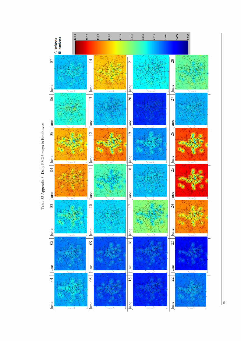
78
Tab
le 3
2 A
pp
end
ix 3
-D
aily
PM
2.5
map
s in
Ein
dh
oven
Jun
e 01
Jun
e 02
Jun
e 03
Jun
e 04
Jun
e 05
Jun
e 06
Jun
e 07
Jun
e 08
Jun
e 09
Jun
e 10
Jun
e 11
Jun
e 12
Jun
e 13
Jun
e 14
Ju
ne
15
Jun
e 16
Jun
e 17
Jun
e 18
Jun
e 19
Jun
e 20
Jun
e 21
Ju
ne
22
Jun
e 23
Jun
e 24
Jun
e 25
Jun
e 26
Jun
e 27
Jun
e 28

79
Tab
le 3
3 A
pp
end
ix 4
-Ho
url
y P
M10 m
aps
for
Jun
e 04 in
Ein
dh
oven
00:0
0-0
1:0
0
Jun
e 4
01:0
0-0
2:0
0
Jun
e 4
02:0
0-0
3:0
0
Jun
e 4
03:0
0-0
4:0
0
Jun
e 4
04:0
0-0
5:0
0
Jun
e 4
05:0
0-0
6:0
0
Jun
e 4
06:0
0-0
7:0
0
Jun
e 4
07:0
0-0
8:0
0
Jun
e 4
08:0
0-0
9:0
0
Jun
e 4
09:0
0-1
0:0
0
Jun
e 4
10:0
0-1
1:0
0
Jun
e 4
11:0
0-1
2:0
0
Jun
e 4
12:0
0-1
3:0
0
Jun
e 4
13:0
0-1
4:0
0
Jun
e 4
14:0
0-1
5:0
0
Jun
e 4
15:0
0-1
6:0
0
Jun
e 4
16:0
0-1
7:0
0
Jun
e 4
17:0
0-1
8:0
0
Jun
e 4
18:0
0-1
9:0
0
Jun
e 4
19:0
0-2
0:0
0
Jun
e 4
20:0
0-2
1:0
0
Jun
e 4
21:0
0-2
2:0
0
Jun
e 4
22:0
0-2
3:0
0
Jun
e 4
23:0
0-2
4:0
0
Jun
e 4

80
Tab
le 3
4 A
pp
end
ix 5
- H
ourl
y P
M2.5
map
s fo
r Ju
ne
04 in
Ein
dh
oven
00:0
0-0
1:0
0
Jun
e 4
01:0
0-0
2:0
0
Jun
e 4
02:0
0-0
3:0
0
Jun
e 4
03:0
0-0
4:0
0
Jun
e 4
04:0
0-0
5:0
0
Jun
e 4
05:0
0-0
6:0
0
Jun
e 4
06:0
0-0
7:0
0
Jun
e 4
07:0
0-0
8:0
0
Jun
e 4
08:0
0-0
9:0
0
Jun
e 4
09:0
0-1
0:0
0
Jun
e 4
10:0
0-1
1:0
0
Jun
e 4
11:0
0-1
2:0
0
Jun
e 4
12:0
0-1
3:0
0
Jun
e 4
13:0
0-1
4:0
0
Jun
e 4
14:0
0-1
5:0
0
Jun
e 4
15:0
0-1
6:0
0
Jun
e 4
16:0
0-1
7:0
0
Jun
e 4
17:0
0-1
8:0
0
Jun
e 4
18:0
0-1
9:0
0
Jun
e 4
19:0
0-2
0:0
0
Jun
e 4
20:0
0-2
1:0
0
Jun
e 4
21:0
0-2
2:0
0
Jun
e 4
22:0
0-2
3:0
0
Jun
e 4
23:0
0-2
4:0
0
Jun
e 4

81