space-based maneuver detection and characterization using
TRANSCRIPT
Air Force Institute of TechnologyAFIT Scholar
Theses and Dissertations Student Graduate Works
3-1-2018
Space-based Maneuver Detection andCharacterization using Multiple Model AdaptiveEstimationJustin D. Katzovitz
Follow this and additional works at: https://scholar.afit.edu/etd
Part of the Astrodynamics Commons, and the Space Vehicles Commons
This Thesis is brought to you for free and open access by the Student Graduate Works at AFIT Scholar. It has been accepted for inclusion in Theses andDissertations by an authorized administrator of AFIT Scholar. For more information, please contact [email protected].
Recommended CitationKatzovitz, Justin D., "Space-based Maneuver Detection and Characterization using Multiple Model Adaptive Estimation" (2018).Theses and Dissertations. 1774.https://scholar.afit.edu/etd/1774

SPACE-BASED MANEUVER DETECTIONAND CHARACTERIZATION USING
MULTIPLE MODEL ADAPTIVEESTIMATION
THESIS
Justin D. Katzovitz, 2d Lt, USAF
AFIT-ENY-MS-18-M-268
DEPARTMENT OF THE AIR FORCEAIR UNIVERSITY
AIR FORCE INSTITUTE OF TECHNOLOGY
Wright-Patterson Air Force Base, Ohio
DISTRIBUTION STATEMENT A. APPROVED FOR PUBLIC RELEASE;
DISTRIBUTION IS UNLIMITED

The views expressed in this thesis are those of the author and do not reflect the officialpolicy or position of the United States Air Force, the United States Department ofDefense or the United States Government. This is an academic work and should notbe used to imply or infer actual mission capability or limitations.
AFIT-ENY-MS-18-M-268
SPACE-BASED MANEUVER DETECTION AND CHARACTERIZATION
USING MULTIPLE MODEL ADAPTIVE ESTIMATION
THESIS
Presented to the Faculty
Department of Aeronautics and Astronautics
Graduate School of Engineering and Management
Air Force Institute of Technology
Air University
Air Education and Training Command
in Partial Fulfillment of the Requirements for the
Degree of Master of Science in Astronautical Engineering
Justin D. Katzovitz, BS
2d Lt, USAF
March 2018
DISTRIBUTION STATEMENT A. APPROVED FOR PUBLIC RELEASE;
DISTRIBUTION IS UNLIMITED

AFIT-ENY-MS-18-M-268
SPACE-BASED MANEUVER DETECTION AND CHARACTERIZATION
USING MULTIPLE MODEL ADAPTIVE ESTIMATION
Justin D. Katzovitz, BS2d Lt, USAF
Approved:
Joshuah A. Hess, PhD (Chairman) Date
Richard G. Cobb, PhD (Member) Date
Kirk W. Johnson, PhD (Member) Date

AFIT-ENY-MS-18-M-268
Abstract
An increasingly congested space environment requires real-time and dynamic space
situational awareness (SSA) on both domestic and foreign space objects in Earth
orbits. Current statistical orbit determination (SOD) techniques are able to esti-
mate and track trajectories for cooperative spacecraft. However, a non-cooperative
spacecraft performing unknown maneuvers at unknown times can lead to unexpected
changes in the underlying dynamics of classical filtering techniques. Adaptive estima-
tion techniques can be utilized to build a bank of recursive estimators with different
hypotheses on a system’s dynamics. The current study assesses the use of a multiple
model adaptive estimation (MMAE) technique for detecting and characterizing non-
cooperative spacecraft maneuvers using space-based sensors for spacecraft in close
proximity. A series of classical and variable state multiple model frameworks are im-
plemented, tested, and analyzed through maneuver detection scenarios using relative
spacecraft orbit dynamics. Variable levels of noise, data availability, and target thrust
profiles are used to demonstrate and quantify the performance of the MMAE algo-
rithm using Monte Carlo methods. The current research demonstrates that adaptive
estimation techniques are able to handle unknown changes in the dynamics while
keeping comparable errors with respect to other classical estimation methods.
iv

To those who made the ultimate sacrifice so others could reach for the stars
Ad Astra Per Aspera
v

Acknowledgements
There are many people that I must recognize without whom I believe this journey
through AFIT and beyond would not be possible.
To my research advisor, Joshuah Hess, who has kept me on track and guided me
through my thesis project every step of the way.
To my instructors and advisors at AFIT and USAFA, who inspire me to continue
learning not just throughout my career but throughout my life.
To my parents, Larry and Kristina, who have provided me with every opportunity
to aspire to greatness and a moral foundation to use that greatness for good.
To my sister, Louise, who excites my inner passion for engineering and constantly
reminds me that I could be making more money in the private sector.
To my lovely wife, Felicia, who not only supports me through the toughest times
but is there to pick me up and celebrate the happiest times.
Justin D. Katzovitz
vi

Table of Contents
Page
Abstract . . . . . . . . . . . . . . . . . . . . . . . . . . . . . . . . . . . . . . . . . . . . . . . . . . . . . . . . . . . . . . . iv
Acknowledgements . . . . . . . . . . . . . . . . . . . . . . . . . . . . . . . . . . . . . . . . . . . . . . . . . . . . . . vi
List of Figures . . . . . . . . . . . . . . . . . . . . . . . . . . . . . . . . . . . . . . . . . . . . . . . . . . . . . . . . . . ix
List of Tables . . . . . . . . . . . . . . . . . . . . . . . . . . . . . . . . . . . . . . . . . . . . . . . . . . . . . . . . . . . . x
List of Acronyms . . . . . . . . . . . . . . . . . . . . . . . . . . . . . . . . . . . . . . . . . . . . . . . . . . . . . . . xii
I. Introduction . . . . . . . . . . . . . . . . . . . . . . . . . . . . . . . . . . . . . . . . . . . . . . . . . . . . . . . . 1
1.1 Motivation . . . . . . . . . . . . . . . . . . . . . . . . . . . . . . . . . . . . . . . . . . . . . . . . . . . . . 11.2 Problem . . . . . . . . . . . . . . . . . . . . . . . . . . . . . . . . . . . . . . . . . . . . . . . . . . . . . . . 31.3 Document Overview . . . . . . . . . . . . . . . . . . . . . . . . . . . . . . . . . . . . . . . . . . . . . 4
II. Literature Review . . . . . . . . . . . . . . . . . . . . . . . . . . . . . . . . . . . . . . . . . . . . . . . . . . . 6
2.1 Statistical Orbit Determination. . . . . . . . . . . . . . . . . . . . . . . . . . . . . . . . . . . . 62.1.1 Applications of Estimation Theory . . . . . . . . . . . . . . . . . . . . . . . . . . . 72.1.2 Least Squares Estimation . . . . . . . . . . . . . . . . . . . . . . . . . . . . . . . . . . 102.1.3 Kalman Filtering . . . . . . . . . . . . . . . . . . . . . . . . . . . . . . . . . . . . . . . . . 122.1.4 The Unscented Kalman Filter . . . . . . . . . . . . . . . . . . . . . . . . . . . . . . 152.1.5 Filter Smoothers . . . . . . . . . . . . . . . . . . . . . . . . . . . . . . . . . . . . . . . . . 16
2.2 Multiple Model Adaptive Estimation . . . . . . . . . . . . . . . . . . . . . . . . . . . . . . 172.2.1 Interacting Multiple Models . . . . . . . . . . . . . . . . . . . . . . . . . . . . . . . . 182.2.2 Variable State Dimension Filter . . . . . . . . . . . . . . . . . . . . . . . . . . . . 19
2.3 Relative Satellite Motion . . . . . . . . . . . . . . . . . . . . . . . . . . . . . . . . . . . . . . . . 232.3.1 Local-Vertical Local-Horizontal Reference Frame . . . . . . . . . . . . . . 232.3.2 The Hill Clohessy Wiltshire Model . . . . . . . . . . . . . . . . . . . . . . . . . . 24
2.4 Space Sensor Analysis . . . . . . . . . . . . . . . . . . . . . . . . . . . . . . . . . . . . . . . . . . . 282.4.1 Space-based Measurements . . . . . . . . . . . . . . . . . . . . . . . . . . . . . . . . 282.4.2 Measurement Collection Techniques . . . . . . . . . . . . . . . . . . . . . . . . . 292.4.3 Measurement Noise . . . . . . . . . . . . . . . . . . . . . . . . . . . . . . . . . . . . . . . 32
2.5 Summary . . . . . . . . . . . . . . . . . . . . . . . . . . . . . . . . . . . . . . . . . . . . . . . . . . . . . 32
III. Methodology . . . . . . . . . . . . . . . . . . . . . . . . . . . . . . . . . . . . . . . . . . . . . . . . . . . . . . 33
3.1 Research Questions Reviewed . . . . . . . . . . . . . . . . . . . . . . . . . . . . . . . . . . . . 333.2 Overview of the Approach . . . . . . . . . . . . . . . . . . . . . . . . . . . . . . . . . . . . . . . 36
3.2.1 Kalman Filter Algorithms . . . . . . . . . . . . . . . . . . . . . . . . . . . . . . . . . 363.2.2 VSD Algorithm . . . . . . . . . . . . . . . . . . . . . . . . . . . . . . . . . . . . . . . . . . 383.2.3 IMM Algorithm . . . . . . . . . . . . . . . . . . . . . . . . . . . . . . . . . . . . . . . . . . 38
vii

Page
3.3 Scenario Simulation . . . . . . . . . . . . . . . . . . . . . . . . . . . . . . . . . . . . . . . . . . . . . 423.3.1 Initial Conditions and Noise Factors . . . . . . . . . . . . . . . . . . . . . . . . 423.3.2 Parameter Study for Maneuver Detection . . . . . . . . . . . . . . . . . . . . 453.3.3 Kalman Filter Validation . . . . . . . . . . . . . . . . . . . . . . . . . . . . . . . . . . 47
3.4 Summary . . . . . . . . . . . . . . . . . . . . . . . . . . . . . . . . . . . . . . . . . . . . . . . . . . . . . 48
IV. Results and Analysis . . . . . . . . . . . . . . . . . . . . . . . . . . . . . . . . . . . . . . . . . . . . . . . . 49
4.1 Maneuver Detection Analysis . . . . . . . . . . . . . . . . . . . . . . . . . . . . . . . . . . . . 504.2 Small Maneuver Analysis . . . . . . . . . . . . . . . . . . . . . . . . . . . . . . . . . . . . . . . . 564.3 Maneuver Characterization Analysis . . . . . . . . . . . . . . . . . . . . . . . . . . . . . . 594.4 Dynamic Thrust Analysis . . . . . . . . . . . . . . . . . . . . . . . . . . . . . . . . . . . . . . . 664.5 Parameter Study Conclusions . . . . . . . . . . . . . . . . . . . . . . . . . . . . . . . . . . . . 694.6 IMM Algorithm Analysis . . . . . . . . . . . . . . . . . . . . . . . . . . . . . . . . . . . . . . . . 704.7 Summary . . . . . . . . . . . . . . . . . . . . . . . . . . . . . . . . . . . . . . . . . . . . . . . . . . . . . 73
V. Conclusions and Recommendations . . . . . . . . . . . . . . . . . . . . . . . . . . . . . . . . . . . 75
5.1 Research Questions Answered . . . . . . . . . . . . . . . . . . . . . . . . . . . . . . . . . . . . 755.2 Research Implications . . . . . . . . . . . . . . . . . . . . . . . . . . . . . . . . . . . . . . . . . . . 765.3 Potential Future Research . . . . . . . . . . . . . . . . . . . . . . . . . . . . . . . . . . . . . . . 785.4 Conclusion . . . . . . . . . . . . . . . . . . . . . . . . . . . . . . . . . . . . . . . . . . . . . . . . . . . . 79
A. Estimation Algorithms . . . . . . . . . . . . . . . . . . . . . . . . . . . . . . . . . . . . . . . . . . . . . . 81
B. Additional Scenarios and Results . . . . . . . . . . . . . . . . . . . . . . . . . . . . . . . . . . . . . 84
C. Nonlinear Dynamical Analysis . . . . . . . . . . . . . . . . . . . . . . . . . . . . . . . . . . . . . . . 89
Bibliography . . . . . . . . . . . . . . . . . . . . . . . . . . . . . . . . . . . . . . . . . . . . . . . . . . . . . . . . . . . 91
viii

List of Figures
Figure Page
1 The Gaussian zero-mean probability density function . . . . . . . . . . . . . . . . . 8
2 VSD filter switching from quiescent model tomaneuvering model . . . . . . . . . . . . . . . . . . . . . . . . . . . . . . . . . . . . . . . . . . . . . 22
3 The LVLH reference frame . . . . . . . . . . . . . . . . . . . . . . . . . . . . . . . . . . . . . . . 24
4 Visual diagram of the VSD IMM algorithm . . . . . . . . . . . . . . . . . . . . . . . . 40
5 Visual diagram of the 1G IMM algorithm . . . . . . . . . . . . . . . . . . . . . . . . . . 41
6 Position errors for maneuver detection scenario 1 with(a) a single VSD filter and (b) IMM VSD filters; dashedlines indicate the target maneuver . . . . . . . . . . . . . . . . . . . . . . . . . . . . . . . . 52
7 For maneuver detection scenario 2 (a) the maneuverdetection statistic and (b) the thrust magnitudeestimate vs truth . . . . . . . . . . . . . . . . . . . . . . . . . . . . . . . . . . . . . . . . . . . . . . . 55
8 Maneuver detection statistic for small maneuverscenario 1 with (a) a single filter and (b) IMM filters;dashed lines indicate the target maneuver . . . . . . . . . . . . . . . . . . . . . . . . . . 57
9 Thrust acceleration estimate for maneuvercharacterization scenario 1 with (a) a single filter and(b) IMM filters . . . . . . . . . . . . . . . . . . . . . . . . . . . . . . . . . . . . . . . . . . . . . . . . . 61
10 Thrust acceleration estimate for maneuvercharacterization scenario 3 with (a) a single filter and(b) IMM filters . . . . . . . . . . . . . . . . . . . . . . . . . . . . . . . . . . . . . . . . . . . . . . . . . 65
11 Thrust acceleration estimate for dynamic thrust scenario . . . . . . . . . . . . . 68
12 Typical model weights for (a) a 1G IMM algorithm and(b) a 2G IMM algorithm; dashed lines indicate thetarget maneuver . . . . . . . . . . . . . . . . . . . . . . . . . . . . . . . . . . . . . . . . . . . . . . . . 71
13 Model weights for (a) maneuver detection scenario 3and (b) maneuver detection scenario 4 . . . . . . . . . . . . . . . . . . . . . . . . . . . . . 73
ix
List of Tables
Table Page
1 Critical values of a chi-square distribution . . . . . . . . . . . . . . . . . . . . . . . . . . 21
2 Common space-based propulsion systems and theirapplications . . . . . . . . . . . . . . . . . . . . . . . . . . . . . . . . . . . . . . . . . . . . . . . . . . . . 34
3 Initial parameters for baseline scenario . . . . . . . . . . . . . . . . . . . . . . . . . . . . 47
4 Simulation results for baseline scenario . . . . . . . . . . . . . . . . . . . . . . . . . . . . 48
5 The algorithms and filters used for each results section . . . . . . . . . . . . . . . 49
6 Initial parameters for maneuver detection scenario 1 . . . . . . . . . . . . . . . . . 50
7 Simulation results for maneuver detection scenario 1 . . . . . . . . . . . . . . . . . 51
8 Initial parameters for maneuver detection scenario 2 . . . . . . . . . . . . . . . . . 53
9 Simulation results for maneuver detection scenario 2 . . . . . . . . . . . . . . . . . 54
10 Initial parameters for small maneuver scenario 1 . . . . . . . . . . . . . . . . . . . . 56
11 Initial parameters for small maneuver scenario 2 . . . . . . . . . . . . . . . . . . . . 58
12 Simulation results for small maneuver scenario 2 . . . . . . . . . . . . . . . . . . . . 59
13 Simulation results for maneuver characterizationscenario 1 . . . . . . . . . . . . . . . . . . . . . . . . . . . . . . . . . . . . . . . . . . . . . . . . . . . . . 60
14 Initial parameters for maneuver characterizationscenario 2 . . . . . . . . . . . . . . . . . . . . . . . . . . . . . . . . . . . . . . . . . . . . . . . . . . . . . 62
15 Simulation results for maneuver characterizationscenario 2 . . . . . . . . . . . . . . . . . . . . . . . . . . . . . . . . . . . . . . . . . . . . . . . . . . . . . 63
16 Initial parameters for maneuver characterizationscenario 3 . . . . . . . . . . . . . . . . . . . . . . . . . . . . . . . . . . . . . . . . . . . . . . . . . . . . . 63
17 Simulation results for maneuver characterizationscenario 3 . . . . . . . . . . . . . . . . . . . . . . . . . . . . . . . . . . . . . . . . . . . . . . . . . . . . . 64
18 Initial parameters for dynamic thrust scenario . . . . . . . . . . . . . . . . . . . . . . 67
19 Simulation results for dynamic thrust scenario . . . . . . . . . . . . . . . . . . . . . . 67
x
Table Page
20 Initial parameters for maneuver detection scenario 3 . . . . . . . . . . . . . . . . . 84
21 Simulation results for maneuver detection scenario 3 . . . . . . . . . . . . . . . . . 85
22 Initial parameters for maneuver detection scenario 4 . . . . . . . . . . . . . . . . . 85
23 Simulation results for maneuver detection scenario 4 . . . . . . . . . . . . . . . . . 86
24 Simulation results for small maneuver scenario 1 . . . . . . . . . . . . . . . . . . . . 86
25 Initial parameters for maneuver characterizationscenario 4 . . . . . . . . . . . . . . . . . . . . . . . . . . . . . . . . . . . . . . . . . . . . . . . . . . . . . 87
26 Simulation results for maneuver characterizationscenario 4 . . . . . . . . . . . . . . . . . . . . . . . . . . . . . . . . . . . . . . . . . . . . . . . . . . . . . 87
27 Simulation results for dynamic thrust scenario 2 . . . . . . . . . . . . . . . . . . . . 88
28 Simulation results for dynamic thrust scenario 3 . . . . . . . . . . . . . . . . . . . . 88
29 Initial parameters for the relative trajectory scenario . . . . . . . . . . . . . . . . 89
30 Simulation results for the relative trajectory scenario . . . . . . . . . . . . . . . . 90
xi

List of Acronyms
U.S. United States
UN United Nations
USAF U.S. Air Force
DoD U.S. Department of Defense
SSA space situational awareness
JSpOC Joint Space Operations Center
SSN Space Surveillance Network
AFSPC Air Force Space Command
NRC National Research Council
UCT uncorrelated target
RPO rendezvous and proximity operations
GEO geosynchronous orbit
SOD statistical orbit determination
MMSE minimum mean square error
LEO low Earth orbit
BLS batch least squares
KF Kalman filter
EKF extended Kalman filter
xii

MMAE multiple model adaptive estimation
IMM interacting multiple models
UKF unscented Kalman filter
UT unscented transformation
FES fixed epoch smoothers
IMM interacting multiple models
PDF probability density function
VSD variable state dimension
MD Mahalanobis distance
ED Euclidean distance
NMC natural motion circumnavigation
ROEs relative orbital elements
EO electro-optical
LIDAR light detection and ranging
IOD initial orbit determination
1G first generation
2G second generation
xiii

SPACE-BASED MANEUVER DETECTION AND CHARACTERIZATION
USING MULTIPLE MODEL ADAPTIVE ESTIMATION
I. Introduction
1.1 Motivation
Since launching the first satellites into Earth orbit, the United States (U.S.) and
its military have treated the space domain as the ultimate high ground [1]. The
space-based technology requirements of today’s world have created an arena of
contest, congestion, and competition among other space-faring nations [2].
Approximately 60 nations as well as a multitude of commercial and academic
satellite operators currently work with thousands of space assets in Earth orbits [3].
The 1974 United Nations (UN) Convention on Registration requires nations
launching objects into space to register basic orbit parameters and general
spacecraft function [4]. Despite providing a symbolic step forward in international
cooperation with regards to the space domain, the required basic orbit parameters
provide little information necessary for accurate and real-time orbit determination
for the growing list of active spacecraft in Earth orbits. In the years since the UN
convention, the U.S. Air Force (USAF) has conducted its own mission to provide
precise tracking of objects in space for its own assets as well as any other man-made
object large enough to track [2].
The U.S. Department of Defense (DoD) and the USAF emphasize continued
research of space situational awareness (SSA) to protect the US and allied space
capabilities from an increasingly congested space environment [3]. From the Joint
1

Space Operations Center (JSpOC) and the dedicated set of ground radar and
electro-optical (EO) sites around the globe that make up the Space Surveillance
Network (SSN), the DoD actively tracks approximately 22,000 objects in Earth
orbits [2]. Current research throughout the USAF focuses on improving the precise
predictions of man-made spacecraft and debris with the primary objective of
collision avoidance [5], but extended efforts must be taken to perform accurate orbit
determination of additional objects in space due to the high level of uncertainty in
the space environment. JSpOC requires constant improvement in SSA algorithms in
order to support the U.S.’s increasingly important mission of protecting its space
assets [6].
National security concerns limit international cooperation with respect to the
current orbits and future maneuver plans of space assets [7]. Without the open
source sharing of precise orbital information or plans to maneuver space assets, the
U.S. and other space-faring nations face an increased risk for spacecraft collisions.
As seen with the 2009 collision of the commercial communications satellite Iridium
33 and the decommissioned Russian military communications satellite Cosmos 2251,
collisions in space can easily turn two highly capable assets into thousands of pieces
of orbital debris. JSpOC uses a collection of astrodynamic algorithms standardized
by Air Force Space Command (AFSPC) and assessed by the National Research
Council (NRC) to track and estimate the location of objects in space and provide
collision warning to any spacecraft at risk [2].
Much of the SSA effort is used to associate ground-based sensor readings with
specific items in the space catalog [2]. When a spacecraft performs an unannounced
maneuver, the errors in sensor measurements become greater than the required
confidence interval of the cataloged object and its original orbit, creating an
uncorrelated target (UCT) in the JSpOC database [2]. More research is needed to
2

improve tracking, prediction, and estimation of non-cooperative spacecraft that
perform unknown maneuvers at unknown times to increase target correlation and
the overall SSA mission [3].
1.2 Problem
This study assesses the detection and characterization of non-cooperative
spacecraft maneuvers with space-based sensors in rendezvous and proximity
operations (RPO) using adaptive estimation techniques. Previous research by Goff
et al. demonstrated the ability to detect and track unknown maneuvers of
non-cooperative spacecraft using ground-based radars [7]. Although adaptive
estimation techniques have claimed to be more effective at detecting and tracking
unknown maneuvers than traditional orbital estimation techniques [8], Goff admits
that future work is necessary to evaluate scenarios where a spacecraft maneuvers
into an area not covered by ground-based radars. The current research applies an
estimation architecture similar to that in [8] using space-based sensors for spacecraft
in geosynchronous orbit (GEO), filling in the limitations of ground-based sensors.
The motivation of this research identifies three potential interests for the
operational use of adaptive estimation techniques for maneuver detection and
characterization. Serving as the single most up-to-date space object tracking
system, JSpOC needs an accurate and robust orbit determination network.
Consistent detection and tracking of orbital maneuvers will improve JSpOC’s ability
to provide early warning prediction of satellite collisions. Detecting maneuvers of
non-cooperative spacecraft will also provide insight to the commercial space
industry, improving the state-of-the-art in orbital estimation for on-orbit rendezvous
and servicing missions. This research also provides an assessment on applications of
space-based assets to the maneuver detection problem, which will provide valuable
3

information to the USAF space acquisition community when applying adaptive
estimation algorithms to future operational space missions. The overall research
objectives of this study are tailored with these interests in mind to provide a clear
path forward in terms of future operational applications.
The study is divided into three research questions focused on examining current
adaptive estimation techniques and applications to relative satellite motion and
proximity operations as well as assessing the performance of an adaptive estimation
algorithm through a realistic parameter study. The following research questions
shall be answered by the conclusion of this study:
• Can adaptive estimation techniques be applied to detect and characterize
non-cooperative spacecraft maneuvers in satellite close proximity operations?
• How do sensor source and type, data rate, maneuver magnitudes, and relative
trajectory affect the performance of an adaptive estimation algorithm?
• For what types of scenarios does an adaptive estimation algorithm fail to
detect a maneuver or fail to characterize an accurate maneuver magnitude?
1.3 Document Overview
This document consists of five chapters, the first of which is an introduction to
the motivation behind this study and its research objectives. Chapter 2 is a
comprehensive literature review on the background, theory, and methodology
behind this research, to include previous research done on statistical orbit
determination (SOD), adaptive estimation, relative satellite motion, and space-based
sensor analysis. Chapter 3 describes the methodology used in this study, presenting
all of the necessary algorithms and equations discussed in Chapter 2 that will form
the foundation for the variety of maneuver detection and characterization scenarios
4

necessary to accurately validate the different adaptive estimation algorithms used in
this study. Chapter 4 contains the results and analysis of each maneuver detection
and characterization scenario along with discussions assessing efficacy, timeliness of
convergence, and comparisons to traditional estimation algorithms. This document
concludes with Chapter 5, which summarizes the study and emphasizes the
significance of the research while providing recommendations for future work.
5
II. Literature Review
The task of detecting maneuvers of non-cooperative spacecraft using adaptive
estimation for RPO scenarios requires an extensive research effort in the areas of
orbit determination, estimation theory, and relative satellite motion. This chapter
reviews relevant literature that provides the groundwork for each topic of interest,
including the derivations of notable equations and algorithms where necessary. This
chapter also emphasizes previous research done in the area of spacecraft maneuver
detection, providing realistic applications of current research into the overall topic of
orbital estimation and tracking.
2.1 Statistical Orbit Determination
SOD is the generalized term used to describe the application of estimation
theory and how to account for errors in observation measurements and uncertainties
in the dynamics for orbit determination. SOD utilizes the principles of estimation
theory through minimizing residual errors while predicting a spacecraft’s orbital
trajectory, often referred to as the states of the system. The principle of a minimum
mean square error (MMSE) estimation algorithm is to take a series of dependent
variables or measurements and produce an approximation of the state variables as
well as a mean squared estimate for the error in each state. In satellite dynamics,
the mean square error estimate produced is represented by the covariance matrix,
which Wiesel defines as the correlation of the error estimate between each state
variable [9]. The following sections supply the theory and basic derivations of each
estimation technique used in this study and their current applications to SOD and
the overall USAF SSA mission.
6
2.1.1 Applications of Estimation Theory
Originally developed by Carl Friedrich Gauss in the early 1800s, estimation
theory uses statistics to estimate the error in a measured variable and correlate the
estimate to a confidence factor for the measured variable. Gauss revolutionized the
field of orbit determination by focusing on minimizing measurement and calculation
errors instead of attempting to find the perfect dynamical equation to represent
orbital motion [10]. Over a century later, the advancement of technology brought
forth new estimation algorithms that take advantage of increasing computational
speed and accuracy. Today, the USAF utilizes modern estimation theory to
minimize observation errors when tracking space objects [2]. Tapley et al. provides
an in-depth analysis at the estimation theory behind SOD and presents a realistic
approach to building an orbit determination problem through defined orbital
dynamics and initializing error and covariance estimates [11]. Before discussing the
theory behind the estimation techniques used in this study, the estimation problem
is defined in terms of the inherent error in a dynamical system as well as the states
that define the system.
Gauss made the assumption that there is no perfect equation to describe the
motion of a system, establishing the need for deterministic estimation theory.
Modern estimation theory makes a second assumption in that there are no perfect
measurements to determine the states of a system, requiring the need for stochastic
estimation theory [9]. Through his founding of probability theory, Gauss defined
imperfections in dynamical systems as random processes, otherwise known as noise
[10]. For most dynamical systems, the noise in a state estimate can be defined by a
normally distributed probability density function, also known as the Gaussian
distribution as shown in Figure 1. Although noise is defined to be a random process,
the assumption that the noise of the error is normally distributed is not only proven
7

by the central limit theorem but is also observed in the real world all the time. A
complete proof of the central limit theorem can be found in [9].
Figure 1. The Gaussian zero-mean probability density function
A state estimate described by Gaussian white noise is fully defined by a mean of
the state, E(x), and a standard deviation of the state, σx. A dataset defined by a
Gaussian distribution implies that approximately 99% of the points in the dataset
are within 3σ of the mean of the set. Using Figure 1 as an example, E(x) = 0 and
σx = 1. Unless otherwise stated, all instances of error in the dynamical and
measurement equations of this study are assumed to be zero-mean, independent,
white Gaussian noise. These assumptions for the current study imply that every
state estimate has a normally distributed error centered about its mean, and each
state error is uncorrelated with any other state error. Noise and errors in the system
are further defined for this study in Chapter 3.
General applications of estimation theory for dynamical systems are built to
estimate states that are related in some way to the variable dynamics of the system,
8

represented by the equations of motion. Wiesel defines a general state vector x,
which defines the states of the system [9]. The system is defined in Equation (2.1)
by a series of differential equations that relate the changes of the state vector over
time, denoted by the generalized function f , and the confidence in the dynamical
model, denoted by the random process w(t)
dx
dt= f (x, t) + w(t). (2.1)
Another way to represent the dynamics is through a state transition matrix.
The state transition matrix relates a previous state vector to a new state vector
separated by some dependent variable, in this case a discrete time step (t2 - t1).
Shown in Equation (2.2), Stengel and other textbooks on estimation theory use the
state transition matrix to define a discrete-time system with process noise [11, 12]
x(t2) = Φ(t2, t1)x(t1) + w(t1) (2.2)
where Φ(t2, t1) is defined as the state transition matrix, which for nonlinear systems
can vary over each update of the state vector. The term for process noise, w(t1), is
considered a disturbance input for the system, and is still assumed to be white
Gaussian noise.
Estimation theory also defines the relationship between the measurements and
the state vector, along with the uncertainties associated with the measurements
[12]. The measurement vector, z(t), is defined in Equation (2.3)
z(t) = y(t) + v(t) = h[x(t)] + v(t). (2.3)
Stengel uses the output vector, y(t), to relate the state vector, x(t), to the
measurement vector, z(t) with the measurement error represented by a noise
9

component, v(t) [12]. The output vector can be any combination of the states that
the user has interest in, which is defined by the measurement basis function, h[x(t)]
[13].
In most cases, it is simple and efficient to define the state vector x as the
position and velocity vector when dealing with particle dynamics. However, it can
be useful and at times necessary to include other pieces of information regarding the
dynamics of the system in the state vector such as coordinate transformations or
osculating orbital elements. As long as the equations of motion can be defined with
respect to the state vector, estimation theory can be used to track the changes to
the state vector and the errors in the estimate of each state in the system.
2.1.2 Least Squares Estimation
Least squares estimation can be traced back to the original foundations of
estimation theory [10]. By using the probability assumptions described in section
2.1.1, Gauss invented the least squares method to obtain orbits on objects with a
limited amount of observations [9]. The main principle of deterministic least squares
is to calculate the estimate state, x, such that the square of the residuals is
minimized. The calculation of the residuals, r, shown in Equation (2.4), is usually
defined as the difference between the observed measurements and the predicted
measurements, described earlier in Section 2.1 as the measurement vector and a
function of the state vector [14]. A full derivation of both the linear and nonlinear
least squares algorithm can be found in Vallado’s text [15].
r = z(t)− y(t) = z(t)− h[x(t)] (2.4)
Although the least squares algorithm is effective in minimizing the residual
error of the system, problems arise with SOD applications in terms of both
10
computational time and accuracy. Every observation available is incorporated into
the least squares algorithm, and the state vector is sized on the order of the number
of measurements. When these measurements are limited, as in the case of Gauss
estimating the orbit of the asteroid Ceres [9], the least squares solution computed
by hand is precise. Over the course of observing a satellite in low Earth
orbit (LEO), however, an increasing number of measurements over time causes the
memory requirements on a program to become significant.
Since the dynamics of an orbit are inherently nonlinear, the forces affecting the
spacecraft at one observation could differ greatly from the forces at another
observation over the course of many orbits around the Earth. This causes problems
in the least squares solution, as the dynamical state model cannot be easily changed
in real-time [14]. As the external forces on a satellite in orbit, such as aerodrag or
the effects of J2, grow increasingly nonlinear, treating older measurements with the
same confidence as newer observations will cause significant errors in the least
square solution [14].
One of the ways to solve the computational time and accuracy issues with the
least squares algorithm is through batch processing. The main idea behind the
batch least squares (BLS) algorithm is to continuously solve the least squares
problem with available data without having to continuously calculate old data.
Vallado provides the framework for solving the least squares problem through batch
processing [15], while Tapley et al. steps through the derivation and application of
the BLS algorithm [11]. This still produces a linearized solution to the nonlinear
problem, so iterating may not converge on a minimized residual solution [15].
The BLS algorithm is a widely used technique for SOD because it is designed to
handle a small number of observations over a significant period of time while still
minimizing the error between the measurements and the state estimate. Since the
11
SSN ground radar system is tasked with tracking tens of thousands of space objects
daily, the JSpOC orbit tracking and SSA missions are a useful application of the
BLS algorithm [2]. Batch processing is used in these instances of SOD, which can
take a series of observations over significant periods of time and fit the data to the
predicted orbit while minimizing the residuals. Although the BLS technique is
useful for a multitude of ground measurements spread out over many orbital
periods, problems arise when system perturbations are not entirely known and are
therefore modeled incompletely [16]. Due to the real-time requirements inherent in
the maneuver detection problem analyzed in the current study, more sequential
estimation methods are required over the BLS algorithm.
2.1.3 Kalman Filtering
A major issue with the least squares estimation technique is that the converged
state and covariance matrix are based on a large batch of data that may have
accumulated error over a prolonged period of time. No matter how accurate the
estimate is, the least squares algorithm is always based on an epoch time and may
not have a precise estimate for any state at a future epoch time. The solution to
these inherent problems is sequential estimation, or computing the best state
estimate of a time-varying process [15]. The Kalman filter (KF) solves the same
least squares problem as BLS, but tries to minimize errors through sequential
estimation [17].
Vallado cites two major differences between the least squares technique and the
KF [15]. First, the KF continuously updates the epoch time, only predicting the
state estimate at a future observation time. Second, the KF keeps all past
information in the current estimate and covariance matrix, eliminating the need to
continuously recalculate any past states or measurements at each time step.
12

The dynamical equations of motion as well as the measurement equations for
orbit mechanics are often nonlinear in nature, and the linear KF is not always
applicable. Therefore, the extended Kalman filter (EKF) is sometimes necessary
[15]. Wright explains that the EKF is more dynamic than the BLS and is more ideal
for orbit determination [18]. The EKF has a similar algorithm as the linear KF, but
uses a Taylor series approximation at each time step in the propagation to
temporarily linearize the dynamics and apply the optimal least squares solution.
Derivations of the linear KF and EKF can be found in many astrodynamics and
estimation textbooks [9, 11, 12] as well as other works utilizing sequential
estimation [13, 19]. Both the KF and the EKF start with an initial guess of the
state and covariance matrix
x(t0) = x0
P(t0) = P0.
(2.5)
Using Equations (2.2) and (2.3) to define the state and measurement equations,
the process and measurement noise are assumed to be independent, zero mean,
normal probability distributions, with covariances shown in Equation (2.6)
p(w) ∼ N(0,Q)
p(v) ∼ N(0,R)
(2.6)
where the process noise covariance , Q, and the measurement noise covariance, R,
are free to change at each time step to represent the confidence in the dynamics or
the data at any time during the propagation of the filter.
13

The first step in the KF is to propagate the state vector from xk−1 to xk
depending on the dynamical equation of the system. The covariance matrix is also
propagated from Pk−1 to Pk based on the mean squared error of the predicted
state. The predicted state, xk, is then corrected by a combination of the
measurement basis function, hk[x−k ], the predicted state covariance matrix, P−k , and
the measurement covariance matrix, Rk. The correction calculation shown in
equation 2.7 is called the Kalman gain. In both the KF and EKF algorithms, the
Kalman gain is calculated by the same equation
Kk = P−k HTk (HkP
−k HT
k + Rk)−1 (2.7)
where the matrix Hk is a linear measurement basis function multiplied by x−k to get
the output vector, y. In Equation (2.7), the − superscript represents the previous
predicted estimate in the algorithm, while the updated state and covariance
estimate shown in Equation (2.8) is represented by the + superscript. The state and
covariance estimate are updated using the same equations for the linear and
nonlinear case.
x+k = x−k + Kk(zk −Hkx
−k ) (2.8a)
P+k = (I−Kkhk[x
−k ])P−k (2.8b)
Notice that the last term in Equation (2.8a) is the residual vector defined in
Equation (2.4), only this time it only represents the residual vector at the specific
time step instead of at every measurement for the least squares algorithm.
Looking back at Equations (2.5) to (2.8b), it would seem that the linear KF
and the EKF follow the exact same algorithm, which during the
14

prediction-correction stage of the algorithm is completely true. The primary
difference between the KF and the EKF is that the EKF must linearize its
dynamics and measurement basis function in order to propagate in discrete time. If
the dynamics follow the generalized functions shown in Equation (2.1) and (2.3),
then the state estimate is propagated by Equation (2.9), and the linearized
measurement basis function is shown in Equation (2.10).
xk =
∫ tk
tk−1
[xk−1]dx+ xk−1 (2.9)
Hk =∂z
∂x−k(2.10)
Using a linearized form of the dynamics and the measurements at each time
step, the EKF can easily transform the nonlinear dynamic systems seen in orbit
mechanics into a simplified model that can be propagated through the KF
algorithm. However, no matter how small the time step, any linearized model of
nonlinear dynamics are bound to have inherent errors, which can be unacceptable
for SOD.
2.1.4 The Unscented Kalman Filter
Accuracy concerns arise with the EKF because the algorithm must differentiate
the measurement and dynamic functions with respect to the state vector in order to
linearize the problem at every time step. Julier and Uhlmann developed a nonlinear
Kalman filter called the unscented Kalman filter (UKF) for improved performance
and accuracy [20]. While the EKF simply linearizes the dynamics of the system
through each step in the estimation, the UKF overcomes the difficulties that arise
from linearization by propagating the mean and covariance of the state vector
15

through nonlinear transformations [21] . Instead of relying on numerical integration
or linearized propagation, the UKF moves a weighted distribution of critical points
based on the current estimate of the covariance matrix. The weighting methods
used in this study for the nonlinear unscented transformation (UT) are outlined in
Section 3.2.1.
As explained in Teixeira et al., the UKF is similar in computational efficiency
and superior in accuracy to the EKF when implemented properly for orbit
determination [22]. In addition, Teixeira et al. conclude that the UKF is able to
converge uniformly better than the EKF for time-sparse measurements [22]. Pardal
et al. also show that the UKF outperforms other filters when observations are less
frequent, specifically testing this hypothesis with pseudo range observations [23].
2.1.5 Filter Smoothers
At the end of each scenario, a backwards smoother applied to the filter can
further improve the estimated state. Wright and Woodburn explore different
combinations of fixed epoch smoothers (FES) with an EKF to improve state
estimates [24]. The FES is ideal for discrete satellite observations used in orbit
estimation; new measurements processed through the EKF in real-time are also
used to recursively update the estimated state and covariance at some previous
epoch time. Helmick et al. examines a fixed-interval smoothing algorithm using an
adaptive estimation framework, which updates all estimates within an interval from
the current estimate [25]. This approach can be costly for orbit estimation in
real-time because the algorithm requires n2 smoothers working in parallel for every
n models.
Another type of smoother developed for the UKF by Sarkka is the unscented
Rauch-Tung-Striebel smoother [26]. Instead of combining the results of a forward
16

running UKF for the backward-working algorithm, a backward smoother is used to
calculate suitable corrections to the forward algorithm. This concept can improve
the state error for scenarios with large nonlinearities and unknown dynamics such as
a maneuver because it can update previously erroneous state estimates with newly
propagated dynamics. However, because these smoothing algorithms require varying
levels of post-processing, they are not ideal for real-time estimation scenarios and
will not be tested in this study.
2.2 Multiple Model Adaptive Estimation
The NRC has expressed the need for considering future research in multiple
model adaptive estimation (MMAE) with regards to the SSA mission and more
specifically maneuver detection [2]. Tracking a non-cooperative spacecraft and
detecting unknown maneuvers requires an adaptive estimation technique because
the noise components of the non-cooperative spacecraft are unknown and must be
estimated. Magill outlines the fundamentals of adaptive estimation and its
applicable derivations [27]. MMAE uses a bank of KFs that all make different
assumptions about the dynamics of the system, specifically in the covariance of the
process noise, Q.
The adaptive framework allows for different ways to account for unexpected
changes in the state or covariance estimates. Each of the filters has a series of
weighting coefficients that can change based on algorithm specific rules regarding
calculations and filter initializations. Li et al. presents an adaptive filter using a
series of UKFs to approximate and adjust the process noise covariance throughout
the propagation of the algorithm [28]. Moose developed an adaptive state estimator
for the general maneuvering target problem and concluded that the adaptive
estimator with a band of KFs is certainly superior to the linear KF [29]. Although
17
proven accurate in estimating uncertainties in the dynamics of the target, the
adaptive estimation technique still must make a series initial guesses on the process
noise covariance matrix. Without interaction, the MMAE could still diverge if the
guesses of the process noise covariances are not accurate.
2.2.1 Interacting Multiple Models
The concept of interacting multiple models (IMM) is used to solve the problem
of poor initial guesses in the adaptive estimation algorithm. Li et al. states that the
IMM method is the prevailing approach to modern maneuvering target tracking
[30]. The IMM combines the inputs of several models at each time step and uses the
statistics of the residuals to weigh the impact of each model at each step. Compared
to the general adaptive estimation method, the IMM algorithm creates a probability
density function (PDF) of the model weights, which produces the converged results
as a combination of multiple models that could be the correct covariance estimate.
The specific IMM algorithm and PDF used in this study are outlined in Section
3.2.3.
When applying general MMAE techniques to filter through unknown
maneuvers, covariance inflation must occur to prevent divergence [31]. Covariance
inflation is the process of assuming no confidence in the dynamical model during the
maneuver so that the measurement basis function can dominate the state estimate
[11]. Through covariance inflation, however, a trade off occurs. A large covariance
causes a high probability of convergence, but also a high chance for errors in the
state estimate. The IMM filter prevents the need for determining optimal covariance
sizes that are only valid for specific dynamical systems by providing a method to
mix different covariance estimates and weighting the results based on the likelihood
probability calculated for each model [32]. For this reason, the IMM method is
18

considered suboptimal because it may not converge on the exact covariance for the
target orbit during maneuver detection, but as Goff shows in [7], the IMM method
is effective in maneuver detection algorithms when limited information is known
about non-cooperative spacecraft maneuvers.
The IMM framework steps closer towards being able to handle the maneuver
detection problem in that it accounts for the uncertainty in the dynamics of the
non-cooperative spacecraft unknown to the observer through adaptive covariance
analysis. However, large changes in the dynamics, such as an unknown active thrust
maneuver at an unknown time, cannot be accounted for simply through covariance
inflation and adaptive estimation.
2.2.2 Variable State Dimension Filter
The variable state dimension (VSD) filter is a solution to handling major
unknown changes in the dynamics of a maneuvering spacecraft. Bar-Shalom et al.
was the first to apply a variable dimension filter to a general maneuver tracking
scenario [33]. The VSD filter is optimal for dealing with unknown maneuvers
because the filter has the ability to add or subtract states based on the deviation of
the estimated state from the measured state, defined earlier as the residual vector.
High residuals are potentially caused by a fundamental error in the equations of
motion of the system, but a VSD that monitors residuals could account for errors by
adding additional states to the state vector (such as a thrust vector) for a spacecraft
changing its dynamics by maneuvering.
Bar-Shalom et al. expand the algorithm of the VSD filter in their text [34]. The
fundamentals of the VSD filter can be structured as any KF previously discussed in
Section 2.1.3. In this case, two filter models are used: the quiescent model, with
states defined as the position and velocity vector of the target, and the maneuvering
19
model, which tracks an acceleration vector as additional states to the system. The
model switching indicator uses a fading memory average of the sequentially
calculated residuals of the filter based on the quiescent model, seen in Equation
(2.11)
Ψk = rTS−1k r (2.11)
where Sk is the covariance matrix of the residual vector, also known as the
measurement covariance. The scalar value defined in Equation (2.11) is known as
the Mahalanobis distance (MD), and is referred to as the maneuver detection
statistic in the current study. Compared to the commonly used Euclidean
distance (ED), the MD takes into account the correlation in the data through the
measurement covariance matrix [35], which allows the estimation algorithm to
converge on a minimized set of residuals without detecting a false maneuver.
The MD value is based on a chi-square distribution, and the maneuver
threshold used to detect the maneuver start and stop times is based on a two-sided
test at a significant level α = 0.0005, which corresponds to a probability of p =
0.999 that the maneuver detection statistic is less than the critical value. Equation
(2.12) shows the chi-square distribution PDF:
PDF(x; k) =xk/2−1e− x/2
2k/2Γ(k2
) . (2.12)
Here x is the maneuver detection statistic, k is the degrees of freedom for the
system, and Γ denotes the gamma function. Table 1 shows the critical values of a
chi-square distribution based on the degrees of freedom for the system. Based on
the critical values for the 4 and 6 degrees of freedom for the states of the system
20
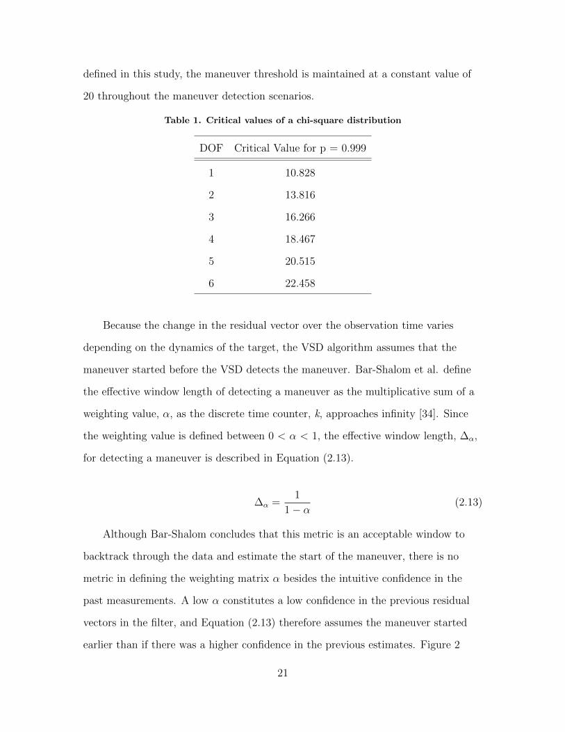
defined in this study, the maneuver threshold is maintained at a constant value of
20 throughout the maneuver detection scenarios.
Table 1. Critical values of a chi-square distribution
DOF Critical Value for p = 0.999
1 10.828
2 13.816
3 16.266
4 18.467
5 20.515
6 22.458
Because the change in the residual vector over the observation time varies
depending on the dynamics of the target, the VSD algorithm assumes that the
maneuver started before the VSD detects the maneuver. Bar-Shalom et al. define
the effective window length of detecting a maneuver as the multiplicative sum of a
weighting value, α, as the discrete time counter, k, approaches infinity [34]. Since
the weighting value is defined between 0 < α < 1, the effective window length, ∆α,
for detecting a maneuver is described in Equation (2.13).
∆α =1
1− α(2.13)
Although Bar-Shalom concludes that this metric is an acceptable window to
backtrack through the data and estimate the start of the maneuver, there is no
metric in defining the weighting matrix α besides the intuitive confidence in the
past measurements. A low α constitutes a low confidence in the previous residual
vectors in the filter, and Equation (2.13) therefore assumes the maneuver started
earlier than if there was a higher confidence in the previous estimates. Figure 2
21
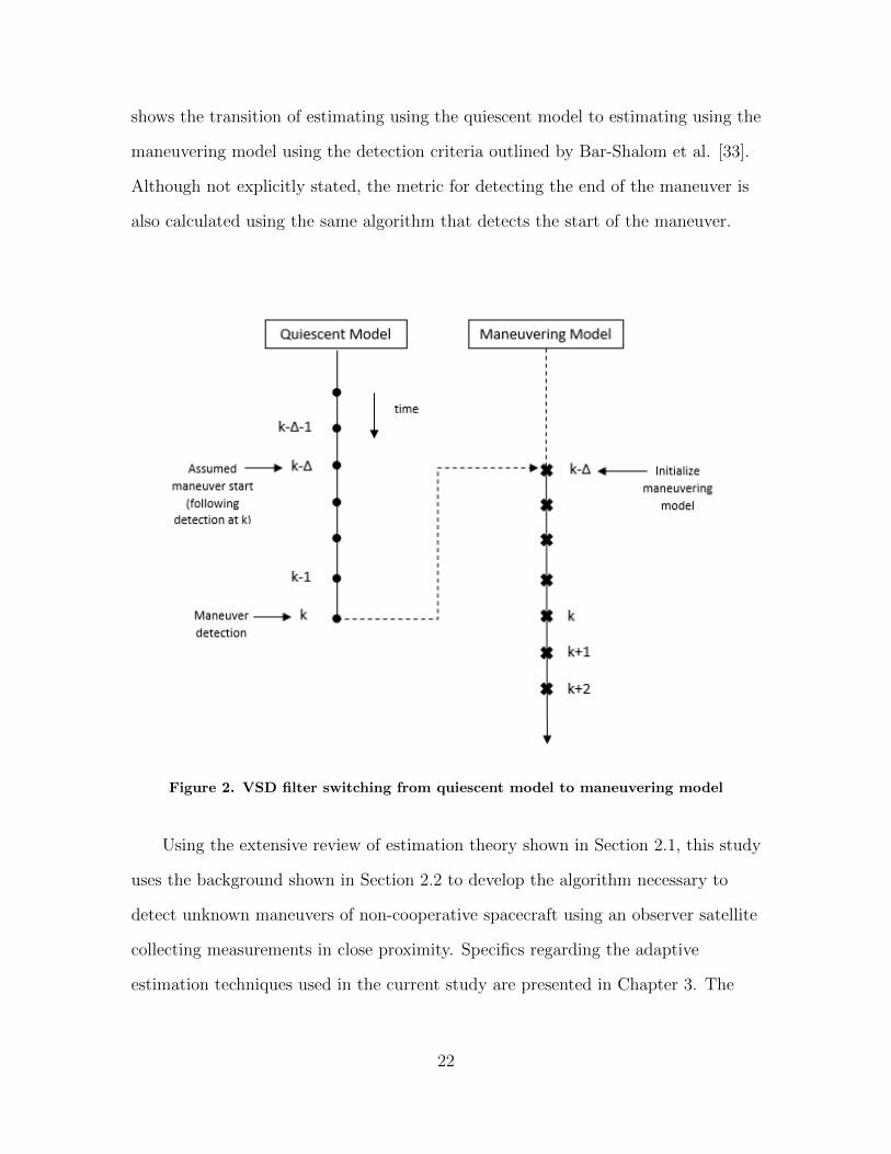
shows the transition of estimating using the quiescent model to estimating using the
maneuvering model using the detection criteria outlined by Bar-Shalom et al. [33].
Although not explicitly stated, the metric for detecting the end of the maneuver is
also calculated using the same algorithm that detects the start of the maneuver.
Figure 2. VSD filter switching from quiescent model to maneuvering model
Using the extensive review of estimation theory shown in Section 2.1, this study
uses the background shown in Section 2.2 to develop the algorithm necessary to
detect unknown maneuvers of non-cooperative spacecraft using an observer satellite
collecting measurements in close proximity. Specifics regarding the adaptive
estimation techniques used in the current study are presented in Chapter 3. The
22

following sections review the necessary background, theory, and equations necessary
to describe the motion of spacecraft flying relative to each other in Earth orbits.
2.3 Relative Satellite Motion
As stated in Section 1.2, this study applies adaptive estimation techniques
discussed in Section 2.2 to RPO scenarios with the objective of non-cooperative
maneuver detection and characterization. The differential equations established in
Equation (2.1) for any estimation algorithm must be able to accurately describe the
dynamics of satellites relative to each other. Relative satellite motion provides a
convenient and efficient method to define the dynamics of RPO spacecraft without
the need for an inertial reference frame.
For every scenario described in this study, consider two satellites in Earth
orbits, one identified as the “chief” and the other identified as the “deputy”. For the
purposes of consistency, the chief in this study is also considered the “observer”, or
the spacecraft taking measurements on the deputy, which will be considered the
“target”. When deriving the equations of motion for RPO scenarios, a new
non-inertial coordinate frame must also be considered to describe the orbit of the
target with respect to the observer.
2.3.1 Local-Vertical Local-Horizontal Reference Frame
As with all dynamical systems, the reference frame used to describe satellite
motion is just as important as the equations of motion themselves. The reference
frame most often used to describe relative satellite motion is the local-vertical
local-horizontal (LVLH) frame, also called the Hill frame for his original derivation
in describing the Moon’s orbit around Earth with respect to the Sun [36]. The
origin of the LVLH frame is centered at the chief, with the x-axis pointing in the
23

direction of the chief’s position vector with respect to the Earth, the z-axis pointing
normal to the orbital plane, and the y-axis completing the right handed coordinate
system. The y-axis is generally pointed in the along-track direction, and if the
chief’s orbit is circular then the y-axis is directly aligned with the chief’s velocity
vector. Figure 3 shows the LVLH reference frame centered at the chief spacecraft,
providing a visual relationship between the states [x,y,x,y] and the space-based
sensor measurements range (ρ), range rate (ρ), and azimuth (α). Further discussion
regarding space-based measurements can be found in Section 2.4.1.
Figure 3. The LVLH reference frame
2.3.2 The Hill Clohessy Wiltshire Model
The Hill Clohessy Wiltshire (HCW) model is the most widely used set of
equations that accurately describe the relative motion of two spacecraft operating in
close proximity. The equations of motion were originally developed by Clohessy and
Wiltshire in 1960 for satellite rendezvous [37] and are similar to Hill’s equations of
24
motion in his lunar theory [36]. Derivations of the HCW equations can be found in
many astrodynamic textbooks [16, 38, 39]. The full nonlinear equations of relative
motion are shown in Equation (2.14)
x− 2ny − ny − n2x− µ
r2=−µr3d
(r + x) + fx (2.14a)
y + 2nx+ nx− n2y =−µr3d
y + fy (2.14b)
z =−µr3d
z + fz (2.14c)
where x, y, and z are the position components; x and y are the velocity components;
and x, y, and z are the acceleration components of the target in the LVLH frame.
The variable r and rd refer to the distance of the chief and deputy with respect to
the Earth, the variables n and n refer to the mean motion of the chief and its first
time derivative, and the variable µ refers to the gravitational constant of the Earth.
The full nonlinear equations of motion are difficult and time consuming to
propagate, and the estimation algorithms presented in Section 2.1 are designed to
handle small unknown errors in the dynamics, which allows for some simplifying
assumptions. The three major assumptions that allow for the full linearized model
of the HCW equations are that the two spacecraft are in Keplerian motion, so the
only force modeled is Earth’s gravitational field as a point mass; the chief is in a
circular orbit, so its mean motion is assumed constant; and the distance between
the satellites is small compared to their orbital radii, so rd ≈ r. For many formation
flying missions in a near-circular orbit and with proper estimation techniques, these
assumptions tend to be valid [13, 40]. The simplified HCW equations are shown in
Equation (2.15):
25
x− 2ny − 3n2x = fx (2.15a)
y + 2nx = fy (2.15b)
z + n2z = fz. (2.15c)
These equations are written in the LVLH reference frame, where x, y, and z are
used to describe the deputy’s position with respect to the chief in the radial,
along-track, and cross-track directions, respectively. The term n in Equation (2.15)
is used to denote the mean motion of the chief, which can be found using the
Earth’s gravitational constant, µ, and the semi-major axis of the chief, ac, as seen in
Equation (2.16)
n =
õ
a3c
. (2.16)
In this study, another simplified nonlinear form of the HCW equations is
explored. The assumptions of Keplerian motion and a circular chief are still valid,
but removing the relative distance assumption allows for scenarios with significant
distances between the chief and the deputy without losing accuracy. The nonlinear
HCW equations without the relative distance assumption are shown in Equation
(2.17).
x− 2ny − n2x− µ
r2=−µr3d
(r + x) + fx (2.17a)
y + 2nx− n2y =−µr3d
y + fy (2.17b)
z =−µr3d
z + fz (2.17c)
26
The right-hand side of Equations (2.14), (2.15), and (2.17) allow for any
external forces acting on the system to be added to the dynamics as a perceived
relative acceleration on the system, which is used in this study as the acceleration
force vector of the deputy when conducting maneuvers.
Assuming the linearized HCW equations of motion shown in Equation (2.15)
have no external forces acting on the system, the analytical solution to the HCW
equations is shown in Equation (2.18)
x =x0
nsin(nt)− (3x0 +
y0
n) cos(nt) + (4x0 +
2y0
n) cos(nt) + (4x0 +
2y0
n) (2.18a)
y =2x0
ncos(nt) + (6x0 +
4y0
n) sin(nt)− (6nx0 + 3y0)t− 2x0
n+ y0 (2.18b)
z =z0
nsin(nt) + z0 cos(nt) (2.18c)
x = x0 cos(nt) + (3nx0 + 2y0) sin(nt) (2.18d)
y = −2x0 sin(nt) + (6nx0 + 4y0) cos(nt)− (6nx0 + 3y0) (2.18e)
z = z0 cos(nt)− nz0 sin(nt) (2.18f)
where x0, y0, etc. are the relative initial conditions of the deputy at some epoch
time, t0. From Equation (2.18e), HCW dynamical system experiences simple
harmonic motion when the following constraint is met:
y0 = −2nx0 (2.19)
Using the constraint from Equation 2.19, the deputy spacecraft follows a
stabilized 2x1 elliptical trajectory relative to the chief, referred to in other RPO
works as natural motion circumnavigation (NMC) [41]. An NMC trajectory is a
27

convenient relative orbit that is used to create initial conditions for the scenarios
presented in this research.
Using the equations of motion outlined in this section, the estimation algorithm
developed in Chapter 3 is able to relate the current states of the system to the
future states of the system in a way that is realistic to the relative satellite motion
aspect of the study. Although there are major assumptions made to simplify the
relative satellite equations of motion, using the process noise covariance analysis
discussed in Section 2.2 can handle errors in the dynamics of the system while still
using the simplifying assumptions in the algorithm. The final equations that are
necessary to the estimation algorithm relate the measurements collected by the
observer on the target to the relative orbital states of the target.
2.4 Space Sensor Analysis
Although the relative satellite motion dynamics defined in Section 2.3 use the
coordinates x, y, and z in the LVLH frame to derive the equations of motion, the
sensor measurements that are fed into the estimation algorithm do not directly
measure position and velocity in LVLH frame coordinates. As mentioned in Section
1.2, this study analyzes an adaptive estimation algorithm against multiple types of
measurements and measurement noise levels to make indications between algorithm
performance and the quality of space-based sensors required. The types of
measurements analyzed in this study are a combination of range-azimuth-elevation
and range-range rate measurements.
2.4.1 Space-based Measurements
Escobal details several techniques for orbit determination using combinations of
available data [42]. A common set of raw measurements obtained from a
28
space-based sensor is range, azimuth, and elevation, defined similarly to ground
based measurements but here in the LVLH frame [13]:
z = h[x(t)] =
ρ
α
ε
LV LH
=
√x2 + y2 + z2
arctan yx
arcsin zρ.
(2.20)
Equation (2.20) is used as the nonlinear measurement basis function to relate the
measurements back to the states of the problem. Another type of space-based
sensor capability to be analyzed in this study is collecting measurements of range
and range rate. This allows us to have some insight into not only the position of the
deputy but also its velocity relative to the chief. The range and range-rate nonlinear
measurement basis function is presented in Equation (2.21) [9]:
z = h[x(t)] =
ρρ
=
√x2 + y2 + z2
xx+yy+zz√x2+y2+z2
. (2.21)
2.4.2 Measurement Collection Techniques
A significant consideration when running estimation algorithms using
space-based measurements outlined in Section 2.4.1 is the frequency of available and
accurate sensor data. Much of this study assumes that sensor data is widely
available on the observer looking at the target, but a space-based environment
breeds a multitude of opportunities for large data errors, especially in
non-cooperative scenarios.
Much of the previous literature on space-based observability analysis focuses on
cooperative measurement collection for formation flying, but many measurement
collection techniques can be applied to a non-cooperative scenario without any
major fundamental technology upgrades. One of the most common approaches to
29
space-based SSA is the angles-only approach because it is useful at gathering
measurements using solely vision-based navigation; Gaias discusses this approach in
a non-cooperative setting using only a space-based camera [43]. Gaias enhances the
accuracy of space-based servicing missions by converting angles-only data into
relative orbital elements (ROEs). However, acquiring range data can be crucial
when dealing with a target in close proximity to the observer, which requires more
complex measurement collection techniques.
Junkins discusses vision-based navigation using a position sensing diode for
RPO [44], but this requires targeting beacons to sense certain wavelengths of light,
which is impossible in the non-cooperative scenario. Whittaker shows that
space-based measurements can be acquired using a photometric sensor to correlate
light intensity with range from the target [45]. Although this technique improves
upon an angles-only approach, it requires reflected light from the Sun as well as
sensor calibrations based on the material properties from the target spacecraft,
which may not be available in a non-cooperative scenario. Krutz analyzes a
radiometric sensor in a space-based mission to detect and track spacecraft debris
[46]. Although this is an ideal non-cooperative scenario, Krutz admits that it would
be difficult to categorize debris solely based on captured light intensity because a
large debris far away would reflect the same amount of energy as a small debris
closer to the observer. All of these EO sensors have inherent blind spots when the
target spacecraft is in between the observer and the Sun, often referred to as the
Sun vector. These EO sensors also require some form of cooperation in order to
acquire accurate range data from the target.
The most common technique for collecting accurate range measurements
without the need for cooperation is a light detection and ranging (LIDAR) sensor
[47, 48]. A LIDAR sensor deploys a laser beam aimed at the target, and the sensor
30

measures the time it takes the reflected beam to return to the observer. Knowing
that the beam travels at the speed of light, the distance traveled can be calculated
by measuring the time traveled round trip between the target and the observer. The
laser range finder is highly accurate because it does not experience atmospheric
scattering in space, and its sensor bandpass is extremely narrow centered on the
laser’s nearly monochromatic wavelength. The effectiveness of a LIDAR device on a
non-cooperative spacecraft lies in the reflectivity of the target’s material at the
laser’s wavelength. However, with a narrow spectral bandwidth and a high powered
laser, the sensor should still detect the laser light reflected off the target without a
large gap in data caused by the Sun vector [48]. Once a range measurement is
confirmed, the range rate measurement is collected by examining the Doppler effect
of the reflected wavelength of the laser beam compared to the wavelength of the
transmitted laser beam [49].
For the non-cooperative space-based RPO scenarios in this study, a realistic
sensor suite for an observer collecting range, range rate, and angles data effectively
would be a combination of EO and LIDAR sensors. In a realistic scenario, an EO
sensor would sweep over a large area until the reflected light from the target
generates relative angle measurements from the observer. As the angle
measurements increased in accuracy, the LIDAR sensor would be able to effectively
point and follow the target, collecting range and range rate data. This study
assumes full measurement knowledge of the target in terms of range, range rate, and
angles data, which implies the initial orbit determination (IOD) on the target is
complete. Although this assumption is highly sensitive to the ability of the observer
to collect accurate and abundant measurements, an in-depth observability analysis
is not performed in this study and is left as future work.
31

2.4.3 Measurement Noise
One of the defining characteristics in assessing algorithm performance is
measurement noise. Applying the current study to the USAF SSA mission requires
accurate estimates in space-based sensor performance. Modern laser range finder
technology developed by Hablani for applications in spacecraft relative navigation
and rendezvous is used as a baseline for realistic assumptions regarding
measurement accuracy and noise [47]. These measurement accuracy values are
compared to previous literature on relative spacecraft estimation [13]. The
measurement noise will be assumed constant throughout each individual scenario,
but the process noise of the algorithm will be estimated by each filter continuously.
Error and noise estimation is outlined in greater detail in Chapter 3.
2.5 Summary
This chapter conducted a review of past and current research efforts in the
areas of orbit determination, estimation theory, adaptive estimation, and relative
satellite motion. Background for the theory necessary to set up the maneuver
detection problem was outlined. Basic derivations of the general equations used in
this study were investigated and presented. Conclusions from the research
completed on the current applications of adaptive estimation algorithms show that
the scenarios developed in this study are unique and will provide a positive
contribution to the areas of study reviewed in this chapter. Further development of
the equations and algorithms used in this study, including specific applications to
maneuver detection scenarios, are discussed in Chapter 3.
32
III. Methodology
This study focuses on investigating adaptive estimation techniques to detect
and characterize spacecraft maneuvers given a set of space-based measurements.
Section 1.2 lists the relevant research questions that will be addressed during this
research. The following chapter outlines the specific procedures and algorithms to
be used, how data will be collected through simulated scenarios, and what analysis
criteria will imply success regarding the research questions defined in this study.
3.1 Research Questions Reviewed
The research questions answered by this study transform the complex problem
of detecting non-cooperative maneuvers using adaptive estimation into a scoped and
logical path forward. The research questions encompass all aspects of assessing a
newly implemented algorithm, including efficacy, performance, and limitations. The
first step before research can begin is to analyze the methodology behind how each
research question can and will be answered to the fullest ability of this study.
The first research question addresses the first and foremost problem when
assessing a new algorithm: efficacy. Does each IMM estimation algorithm work as
anticipated, and what are specific requirements placed on each algorithm in order to
guarantee success? For this first problem, realistic parameters in each maneuver
detection scenario, such as availability of measurement data, will be adjusted for the
sake of efficacy. Scenario parameters will continue to have fewer simplifying
assumptions as the research progresses to assess performance and failure modes.
The MMAE algorithm that detects a spacecraft maneuver for the simplest case is
sufficient for completing the first research question, but success in the simplest case
may not provide adequate data with regards to performance.
33
The second research question lists specific variables that will be used to assess
the performance of each adaptive estimation algorithm. Sensor source relates to
different types of measurement data available in an RPO scenario as well as realistic
estimates for measurement noise to be implemented based on the current
space-based sensor technology available. Hablani’s patent for a space-based laser
range finder has a convenient table for the expected level of noise in the output of
the sensor [47], which will produce range, azimuth, and range rate data on the
target satellite.
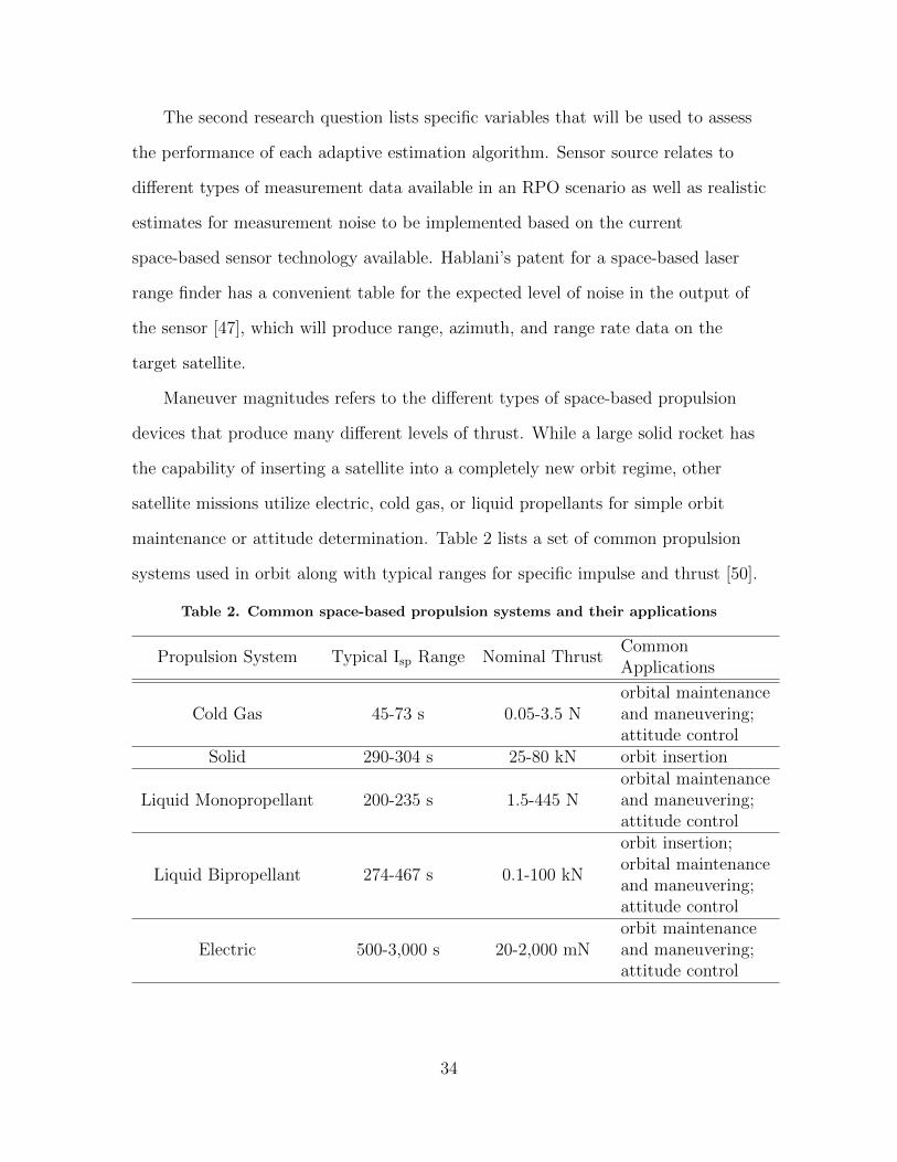
Maneuver magnitudes refers to the different types of space-based propulsion
devices that produce many different levels of thrust. While a large solid rocket has
the capability of inserting a satellite into a completely new orbit regime, other
satellite missions utilize electric, cold gas, or liquid propellants for simple orbit
maintenance or attitude determination. Table 2 lists a set of common propulsion
systems used in orbit along with typical ranges for specific impulse and thrust [50].
Table 2. Common space-based propulsion systems and their applications
Propulsion System Typical Isp Range Nominal ThrustCommonApplications
Cold Gas 45-73 s 0.05-3.5 Norbital maintenanceand maneuvering;attitude control
Solid 290-304 s 25-80 kN orbit insertion
Liquid Monopropellant 200-235 s 1.5-445 Norbital maintenanceand maneuvering;attitude control
Liquid Bipropellant 274-467 s 0.1-100 kN
orbit insertion;orbital maintenanceand maneuvering;attitude control
Electric 500-3,000 s 20-2,000 mNorbit maintenanceand maneuvering;attitude control
34

The data presented in Table 2 will provide a realistic set of maneuver
magnitudes to be utilized in developing scenarios to test each adaptive estimation
algorithm. Nominal thrust calculations for space-based propulsion systems are
measured in Newtons, which allows the spacecraft user to calculate an applied force
on the spacecraft. However, the dynamical equations used to propagate the
estimation algorithms, as seen in Equation (2.15), are the second time derivative of
the state vector, which conceptually is the acceleration of the target with respect to
the observer. When estimating the thrust vector throughout each maneuver
detection scenario, it is not in fact the applied force on the target spacecraft but the
perceived acceleration of the target in the LVLH coordinate frame centered on the
observer. Given mass and propulsion information about the target, an applied
thrust could be derived from the maneuver magnitudes characterized in each
scenario.
The third parameter that will be used for assessing algorithm performance is
the relative trajectory of the target satellite. As stated in Section 2.3.2, the HCW
equations of motion assume that the deputy satellite is relatively close to the chief
satellite [37]. Although there is no explicit distance for divergence of the dynamics,
the further away the deputy gets from the target the less accurate the dynamical
model becomes. A large relative trajectory becomes a problem for the estimator
because the process noise continues to grow as the confidence in the dynamics fades,
until the point where the covariance of the process noise no longer accurately
describes the standard deviation of the estimate from the dynamics [9].
Vallado notes that significant errors are presented for maneuver detection when
using traditional least squares or filter techniques on orbital data because of a lack
of dynamical knowledge during and post-maneuver [15]. Goff concludes that the
MMAE algorithm outperforms all other traditional estimation routines by a factor
35
of 700 in maneuver detection scenarios over the course of just one orbit [7]. This
study will assess these claims for the application of the adaptive algorithm using
space-based maneuver detection scenarios.
Much of the data that assess the performance of the adaptive estimation
algorithm also answers the third research question: at what point does the
algorithm fail to converge on a solution? Many of these limitations are answered
previously, such as the minimum thrust that is able to be detected accurately or the
maximum distance away from the target where space-based measurements become
unrealistic. Another area of performance considered for the third question is the
availability of data for the observer. Through answering the first research question,
the adaptive estimation algorithm will be proven valid with unlimited measurements
on the target at all times throughout each scenario. This simplifying assumption is
not only unchallenging but also unrealistic. Through answering the third research
question, assessments will be made on the sparsity of the measurement data while
still proving algorithm success.
3.2 Overview of the Approach
In order to sufficiently answer all parts of the research questions detailed in
Section 3.1, an in-depth analysis on how the MMAE algorithm is used in this study
must be conducted. Chapter 2 reviewed the background behind MMAE and the
foundations of the VSD filter, but the specific design of the algorithm used in this
study is presented here.
3.2.1 Kalman Filter Algorithms
As discussed in Sections 2.1.3 and 2.1.4, tracking a target in real-time with
nonlinear measurements shown in Equations (2.20) and (2.21) requires a nonlinear
36
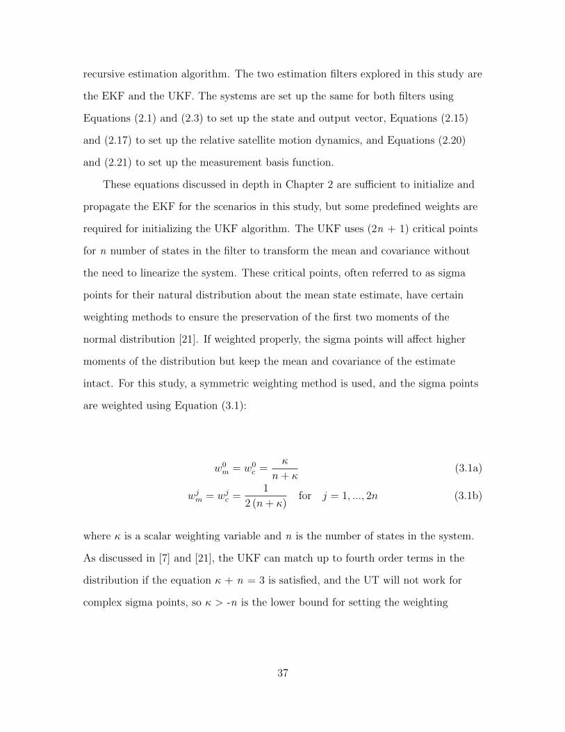
recursive estimation algorithm. The two estimation filters explored in this study are
the EKF and the UKF. The systems are set up the same for both filters using
Equations (2.1) and (2.3) to set up the state and output vector, Equations (2.15)
and (2.17) to set up the relative satellite motion dynamics, and Equations (2.20)
and (2.21) to set up the measurement basis function.
These equations discussed in depth in Chapter 2 are sufficient to initialize and
propagate the EKF for the scenarios in this study, but some predefined weights are
required for initializing the UKF algorithm. The UKF uses (2n + 1) critical points
for n number of states in the filter to transform the mean and covariance without
the need to linearize the system. These critical points, often referred to as sigma
points for their natural distribution about the mean state estimate, have certain
weighting methods to ensure the preservation of the first two moments of the
normal distribution [21]. If weighted properly, the sigma points will affect higher
moments of the distribution but keep the mean and covariance of the estimate
intact. For this study, a symmetric weighting method is used, and the sigma points
are weighted using Equation (3.1):
w0m = w0
c =κ
n+ κ(3.1a)
wjm = wjc =1
2 (n+ κ)for j = 1, ..., 2n (3.1b)
where κ is a scalar weighting variable and n is the number of states in the system.
As discussed in [7] and [21], the UKF can match up to fourth order terms in the
distribution if the equation κ + n = 3 is satisfied, and the UT will not work for
complex sigma points, so κ > -n is the lower bound for setting the weighting
37

variable. Therefore, for all of the orbit estimation scenarios run in this study, we
will set κ = 3 - n for n states.
An extensive step by step algorithm for both the EKF and UKF used in this
study can be found in Appendix A, and many other research in this topic derive
similar algorithms: the EKF in [7] and [11], and the UKF in [7] and [51].
3.2.2 VSD Algorithm
The adaptability of the VSD filter is pivotal in the maneuver detection process.
As stated in Section 2.2.2, the VSD filter accounts for major changes in the
dynamical system by adding or removing states from the equations of motion.
Within the scope of this study, the only states being added in the VSD filter are the
two components of the thrust vector during the maneuver of the target, assuming
in-plane motion. The algorithm also makes the assumption that the thrust vector is
constant throughout each maneuver detection scenario. This causes some inherent
error in the thrust estimate because the acceleration of the target due to a constant
thrust changes slightly over time based on the mass lost by burning propellant. For
the purposes of this study, the thrust states are assumed constant, and for most
scenarios the target is assumed to produce a constant acceleration due to thrust.
Although the fact that the target is maneuvering is tracked by the VSD filter, more
specific parameters such as an estimate for the thrust magnitude and the process
noise of the new dynamics is more accurately estimated through a multiple model
framework.
3.2.3 IMM Algorithm
The IMM algorithm is used in this study to effectively estimate the process
noise of the new dynamics applied during a detected maneuver. A more accurate
38

assessment of this process noise allows for a more accurate representation of the
thrust magnitude and the amount of time spent maneuvering. As discussed in
Section 2.2.1, the IMM framework allows a band of VSD filters with different noise
assumptions to estimate the future state of the system simultaneously. The
interacting component of the algorithm compares the estimates from every VSD in
a PDF, finding a combination of the most likely estimate based on the minimization
of the MD shown in Equation (2.11). A multivariate normal PDF is used in this
study to calculate the model likelihood, and the probability update function is
shown in Equation (3.2) [30]:
Λki = N
(νki ; 0,Ski
)=
1√|2πSki |
e−12 (νki )
T(Sk
i )−1νki (3.2a)
µki =µki−1Λk
i
N∑j=1
µji−1Λji
. (3.2b)
Here Λki is the model likelihood and µki is the model weight for each model k at time
ti. After each model weight is calculated, the weighted state, covariance, and MD at
time ti are calculated using Equation (3.3) [30].
xi =N∑k=1
µki xki Ψi =
N∑k=1
µki Ψki (3.3a)
Pi =N∑k=1
µki
[Pki +
(xki − xi
) (xki − xi
)T](3.3b)
where xki and Pki are the updated state and covariance for each model k at time ti.
This study will look at two different methods for updating the model weights for the
IMM algorithm. For the full interacting method using the VSD in real-time, the
39
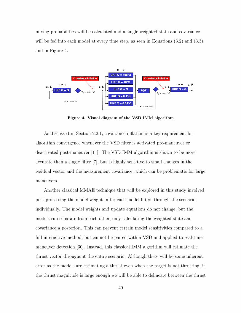
mixing probabilities will be calculated and a single weighted state and covariance
will be fed into each model at every time step, as seen in Equations (3.2) and (3.3)
and in Figure 4.
Figure 4. Visual diagram of the VSD IMM algorithm
As discussed in Section 2.2.1, covariance inflation is a key requirement for
algorithm convergence whenever the VSD filter is activated pre-maneuver or
deactivated post-maneuver [11]. The VSD IMM algorithm is shown to be more
accurate than a single filter [7], but is highly sensitive to small changes in the
residual vector and the measurement covariance, which can be problematic for large
maneuvers.
Another classical MMAE technique that will be explored in this study involved
post-processing the model weights after each model filters through the scenario
individually. The model weights and update equations do not change, but the
models run separate from each other, only calculating the weighted state and
covariance a posteriori. This can prevent certain model sensitivities compared to a
full interactive method, but cannot be paired with a VSD and applied to real-time
maneuver detection [30]. Instead, this classical IMM algorithm will estimate the
thrust vector throughout the entire scenario. Although there will be some inherent
error as the models are estimating a thrust even when the target is not thrusting, if
the thrust magnitude is large enough we will be able to delineate between the thrust
40

vector outputted by the target and the ambient noise of the estimator. The full step
by step IMM algorithm used in this study can be found in Appendix A.
For the purposes of this research and relating to the IMM algorithm analysis in
[30], the classical post-processing IMM algorithm is referred to as the first
generation (1G) IMM algorithm, while the full VSD IMM algorithm is referred to as
the second generation second generation (2G) IMM algorithm. A visual
representation of the 1G IMM algorithm can be seen in Figure 5.
Figure 5. Visual diagram of the 1G IMM algorithm
As shown in both Figure 4 and Figure 5, the IMM framework utilizes five
models with process noise covariance hypotheses varying at orders of magnitude
from the adjacent models in the framework. The number of models and the
distribution of hypotheses is taken from previous research [7], and for each specific
scenario the central process noise covariance is adjusted to ensure improved
interaction of the models and overall convergence of each algorithm. Although this
framework allows for a wider range of estimates regarding the confidence in the
dynamics of the system, there is still the risk of the algorithm diverging if the actual
process noise is outside the range of noise estimates made in the filter models.
Analysis regarding the number of models and the distribution of the hypotheses for
each model in the IMM algorithm is beyond the scope of this study. More analysis
41

regarding algorithm convergence based on the assumptions of each scenario is
discussed in Chapter 4.
3.3 Scenario Simulation
The following sections discuss how each of the RPO scenarios examined in this
study will be initialized, validated, and analyzed within the scope of this study. The
scenarios assessed for this research are run using a coding framework written in
MATLAB. For the sake of continuity between the algorithm, code, and post
analysis, unless otherwise stated, all measurements and estimates are presented in
meters, meters per second, or meters per second per second when describing relative
position, velocity, and acceleration, respectively.
3.3.1 Initial Conditions and Noise Factors
Each scenario initializes in the LVLH frame centered on an observer in a
circular GEO orbit with a semi-major axis of a = 4.2164×10⁷ m. This orbit has a
period of T = 86164 sec (24 hrs), and a constant mean motion of n = 7.2921×10⁻⁵
rad/sec. For most scenarios, the target spacecraft starts in an NMC around the
chief and is assumed to exhibit no out of plane motion. The initial state vector used
for the estimation algorithm is shown in Equation (3.4a), and the state vector for
the VSD is shown in Equation (3.4b):
x = [x0, y0, x0, y0]T (3.4a)
x = [x, y, x, y, Tx, Ty]T . (3.4b)
42

Here x and y represent the radial and along-track position of the target with respect
to the observer, and Tx and Ty refer to the relative thrust acceleration vector of the
target. The state vector is initialized using the conditions shown in Equation (3.5)
represent an NMC starting in the radial direction:
x0 = x0 y0 = 0
x0 = 0 y0 = −2nx0.
(3.5)
where the initial position in the radial direction, x0, is defined in this study as the
relative trajectory parameter. To ensure convergence of the estimator for each
scenario, a large covariance matrix is initialized. The initial state estimation error is
assumed to be 10% of the nominal values, with the initial covariance matrix shown
in Equation (3.6) [13]:
P0 =
σ2xx 0 0 0
0 σ2yy 0 0
0 0 σ2xx 0
0 0 0 σ2yy
=
(0.1n
)2m2 0 0 0
0(
0.1n
)2m2 0 0
0 0 0.12 m2
sec20
0 0 0 0.12 m2
sec2
. (3.6)
Each σ is the standard deviation of each respective state, and n is the mean motion
of the chief spacecraft. Because the covariance matrix is constantly updated
through each time step as seen in Equation (2.8b), the initial covariance is not as
significant as other parameters when analyzing the sensitivity of the estimation
algorithm. This initial covariance is used in all of the scenarios demonstrated in this
study unless otherwise stated that covariance inflation is necessary for convergence.
The last two parameters needed to initialize the estimator are the process noise
and the measurement noise. The measurement noise covariance is initialized based
43

on the types of measurements used in each scenario. Equation (3.7) shows the
different measurement basis functions that will be tested in this study as well as
their corresponding measurement noise covariances.
y =
ρα
=
√x2 + y2
arctan yx
Ri =
ρ ∗ σ2ρ 0
0 σ2α
(3.7a)
y =
ρρ
=
√x2 + y2
xx+yy√x2+y2
Ri =
ρ ∗ σ2ρ 0
0 ρ ∗ σ2ρ
(3.7b)
y =
ρ
ρ
α
=
√x2 + y2
xx+yy√x2+y2
arctan yx
Ri =
ρ ∗ σ2
ρ 0 0
0 ρ ∗ σ2ρ 0
0 0 σ2α
(3.7c)
Each σ corresponds to the standard deviation of the respective measurement. Each
range and range rate covariance is scaled by the range measurement itself, relating
to the assumption that the accuracy of a range sensor is inversely proportional to
the relative distance from the observer to the target [13].
For this study, the process noise covariance is initialized using a single variable,
which simplifies the tuning of this highly sensitive noise factor. The initial process
noise covariance is shown in Equation (3.8):
Q = q0I4X4. (3.8)
Here q0 is a scaling factor that is analyzed and tuned for nearly every scenario to
ensure the convergence of the error residual. For the purposes of this study, the Q
matrix is assumed to be constant once initialized, but the IMM algorithm will
44

attempt to characterize changes in the process noise by making multiple hypotheses
for the Q matrix in each model of the IMM algorithm.
3.3.2 Parameter Study for Maneuver Detection
The IMM algorithm is tested and analyzed using a variety of parameters than
constitute different types of orbits and maneuvers that a target could exhibit with
respect to the observer. The parameters that are analyzed in this study are relative
trajectory, maneuver thrust magnitudes, data rate, data type, and measurement
noise. For each of these parameters, three nominal values are presented with the
hypotheses of good, medium, and poor algorithm performance.
As shown in Equation (3.5), the relative trajectory of the target is expressed in
the initial radial position for each scenario. The nominal values for this parameter
used in this study are shown in Equation (3.9):
x0 =
100 m
1000 m
10000 m
. (3.9)
For the maneuver magnitude parameter, there is no hypothesis relating to the
performance of the IMM algorithm, but rather a small, medium, and large
maneuver. Although this parameter relates to the magnitude of the thrust, the
thrust vector itself may change for each scenario, which should not affect
performance. The maneuver magnitude nominal values are shown in Equation
(3.10):
T =√T 2x + T 2
y =
0.001 m
sec2
0.01 msec2
0.1 msec2
. (3.10)
45

The data rate parameter constitutes the frequency at which measurements are
collected and read into the estimator. Although Section 2.4.2 discussed instances of
large data gaps in an RPO scenario, for the purposes of this study the data rate is
assumed to be constant. The data rate nominal values are shown in Equation
(3.11), here represented as a time gap between each measurement:
δt = ti − ti−1 =
1 sec
10 sec
120 sec
. (3.11)
The data types that form the measurement basis function for each scenario are
shown in Equation (3.7), but the measurement noise covariances are defined by
Equation (3.12) in terms of a good, average, and poor sensor. The good sensor is
related to notional values in [13] meant to represent 1 cm of error and 0.1 cm of
error in the range and range rate measurements, respectively. Each worsening
sensor is simply given an order of magnitude of increasing error.
σgood =
1× 10⁻⁵ m
1× 10⁻⁶ msec
0.05o
σaverage =
1× 10⁻⁴ m
1× 10⁻⁵ msec
0.10o
σpoor =
1× 10⁻³ m
1× 10⁻⁴ msec
0.25o
(3.12)
Within the scope of this research, these notional error values do not relate in
any way to any operational space-based sensor performances. Each sensor is given a
nominal deviation for range, range rate, and azimuth measurements, but each
scenario will use the proper deviation values depending on what data types are
available.
46
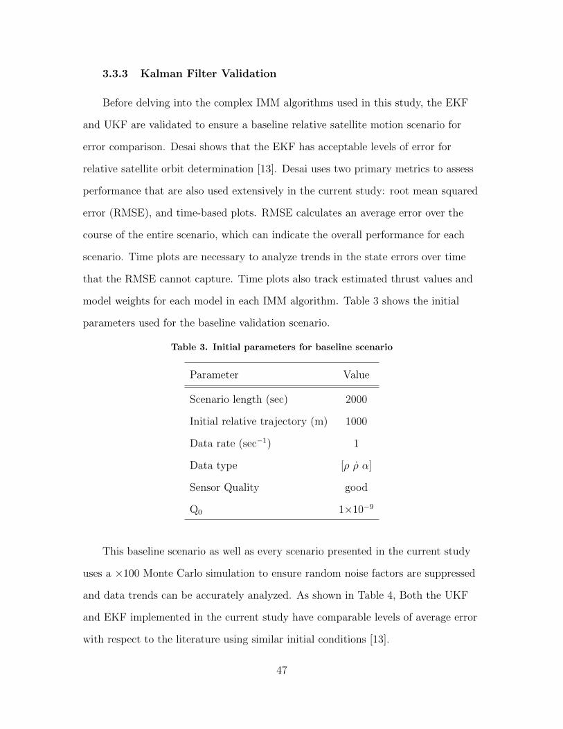
3.3.3 Kalman Filter Validation
Before delving into the complex IMM algorithms used in this study, the EKF
and UKF are validated to ensure a baseline relative satellite motion scenario for
error comparison. Desai shows that the EKF has acceptable levels of error for
relative satellite orbit determination [13]. Desai uses two primary metrics to assess
performance that are also used extensively in the current study: root mean squared
error (RMSE), and time-based plots. RMSE calculates an average error over the
course of the entire scenario, which can indicate the overall performance for each
scenario. Time plots are necessary to analyze trends in the state errors over time
that the RMSE cannot capture. Time plots also track estimated thrust values and
model weights for each model in each IMM algorithm. Table 3 shows the initial
parameters used for the baseline validation scenario.
Table 3. Initial parameters for baseline scenario
Parameter Value
Scenario length (sec) 2000
Initial relative trajectory (m) 1000
Data rate (sec−1) 1
Data type [ρ ρ α]
Sensor Quality good
Q0 1×10⁻⁹
This baseline scenario as well as every scenario presented in the current study
uses a ×100 Monte Carlo simulation to ensure random noise factors are suppressed
and data trends can be accurately analyzed. As shown in Table 4, Both the UKF
and EKF implemented in the current study have comparable levels of average error
with respect to the literature using similar initial conditions [13].
47
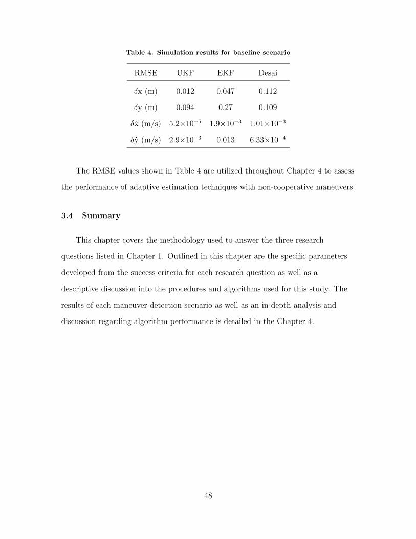
Table 4. Simulation results for baseline scenario
RMSE UKF EKF Desai
δx (m) 0.012 0.047 0.112
δy (m) 0.094 0.27 0.109
δx (m/s) 5.2×10⁻⁵ 1.9×10⁻³ 1.01×10⁻³
δy (m/s) 2.9×10⁻³ 0.013 6.33×10⁻⁴
The RMSE values shown in Table 4 are utilized throughout Chapter 4 to assess
the performance of adaptive estimation techniques with non-cooperative maneuvers.
3.4 Summary
This chapter covers the methodology used to answer the three research
questions listed in Chapter 1. Outlined in this chapter are the specific parameters
developed from the success criteria for each research question as well as a
descriptive discussion into the procedures and algorithms used for this study. The
results of each maneuver detection scenario as well as an in-depth analysis and
discussion regarding algorithm performance is detailed in the Chapter 4.
48
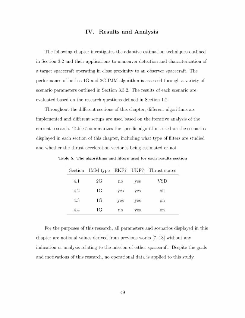
IV. Results and Analysis
The following chapter investigates the adaptive estimation techniques outlined
in Section 3.2 and their applications to maneuver detection and characterization of
a target spacecraft operating in close proximity to an observer spacecraft. The
performance of both a 1G and 2G IMM algorithm is assessed through a variety of
scenario parameters outlined in Section 3.3.2. The results of each scenario are
evaluated based on the research questions defined in Section 1.2.
Throughout the different sections of this chapter, different algorithms are
implemented and different setups are used based on the iterative analysis of the
current research. Table 5 summarizes the specific algorithms used on the scenarios
displayed in each section of this chapter, including what type of filters are studied
and whether the thrust acceleration vector is being estimated or not.
Table 5. The algorithms and filters used for each results section
Section IMM type EKF? UKF? Thrust states
4.1 2G no yes VSD
4.2 1G yes yes off
4.3 1G yes yes on
4.4 1G no yes on
For the purposes of this research, all parameters and scenarios displayed in this
chapter are notional values derived from previous works [7, 13] without any
indication or analysis relating to the mission of either spacecraft. Despite the goals
and motivations of this research, no operational data is applied to this study.
49

4.1 Maneuver Detection Analysis
This section applies a 2G IMM algorithm using VSD filters with varying levels
of process noise to detect and characterize a continuous maneuver in relative
spacecraft motion. Because of the highly nonlinear aspects of the VSD IMM
framework, the EKF was unable to converge for these scenarios. Therefore, the
UKF is the only filter presented with the VSD IMM algorithm.
The first scenario shows a comparison between a single VSD filter and a bank of
VSD filters in an IMM framework. Both scenarios run a single UKF before the
detected maneuver start time and after the detected maneuver stop time. The VSD
filter estimates the thrust acceleration in both the radial and along-track directions
with respect to the observer. The parameters for the first scenario are shown in
Table 6.
Table 6. Initial parameters for maneuver detection scenario 1
Parameter Value
Thrust acceleration (mm/s2) 100
Thrust duration (s) 100
Scenario length (s) 1500
Initial relative trajectory (m) 1000
Data rate (sec−1) 1
Data type [ρ α]
Sensor Quality good
Q0 1×10⁻¹⁰
Table 7 shows the RMSE values in the first maneuver detection scenario for a
single VSD filter compared to a bank of VSD filters in an IMM framework. Both
techniques have zero or minimal error in detecting the maneuver start time and
50

estimating maneuver duration, which can be attributed to a high immediate change
in the dynamics caused by a large target maneuver. Both techniques also converge
on an accurate thrust acceleration vector for the 100 seconds that the VSD filters
are active.
Table 7. Simulation results for maneuver detection scenario 1
RMSE Single UKF IMM UKF
δx (m) 1.23×10³ 0.35
δy (m) 4.26×10³ 0.19
δx (m/s) 1.97 0.011
δy (m/s) 6.54 0.049
δT (m/s2) 6.01×10⁻⁴ 5.03×10⁻⁴
Man start (s) 0 0
Man duration (s) 1.78 0
The IMM VSD algorithm holds RMSE values comparable to the baseline
scenario, while the single VSD filter has RMSE position values on the order of
kilometers. Figure 6a shows that the position errors using a single VSD filter
increase through the maneuver and continue to increase post maneuver, while
Figure 6b shows that the position errors using the VSD filter with an IMM
framework stabilize or decrease post-maneuver.
51
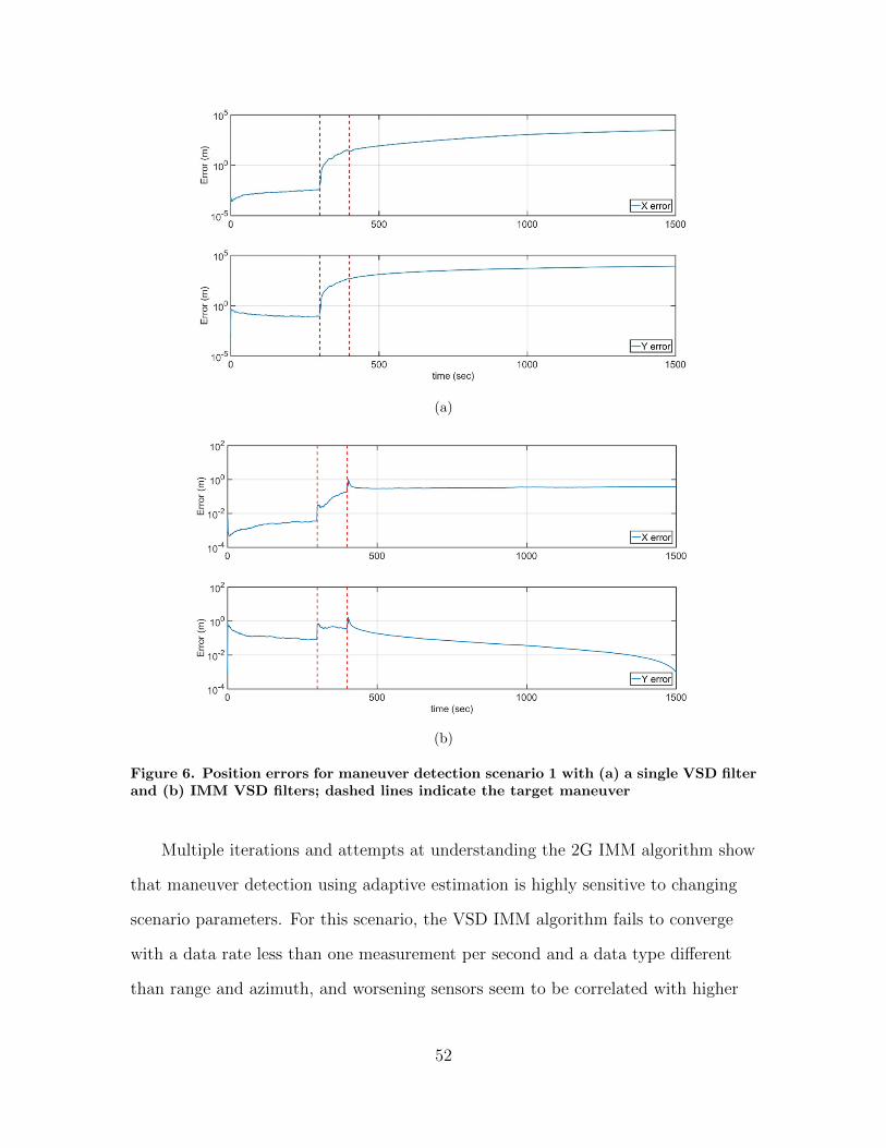
(a)
(b)
Figure 6. Position errors for maneuver detection scenario 1 with (a) a single VSD filterand (b) IMM VSD filters; dashed lines indicate the target maneuver
Multiple iterations and attempts at understanding the 2G IMM algorithm show
that maneuver detection using adaptive estimation is highly sensitive to changing
scenario parameters. For this scenario, the VSD IMM algorithm fails to converge
with a data rate less than one measurement per second and a data type different
than range and azimuth, and worsening sensors seem to be correlated with higher
52
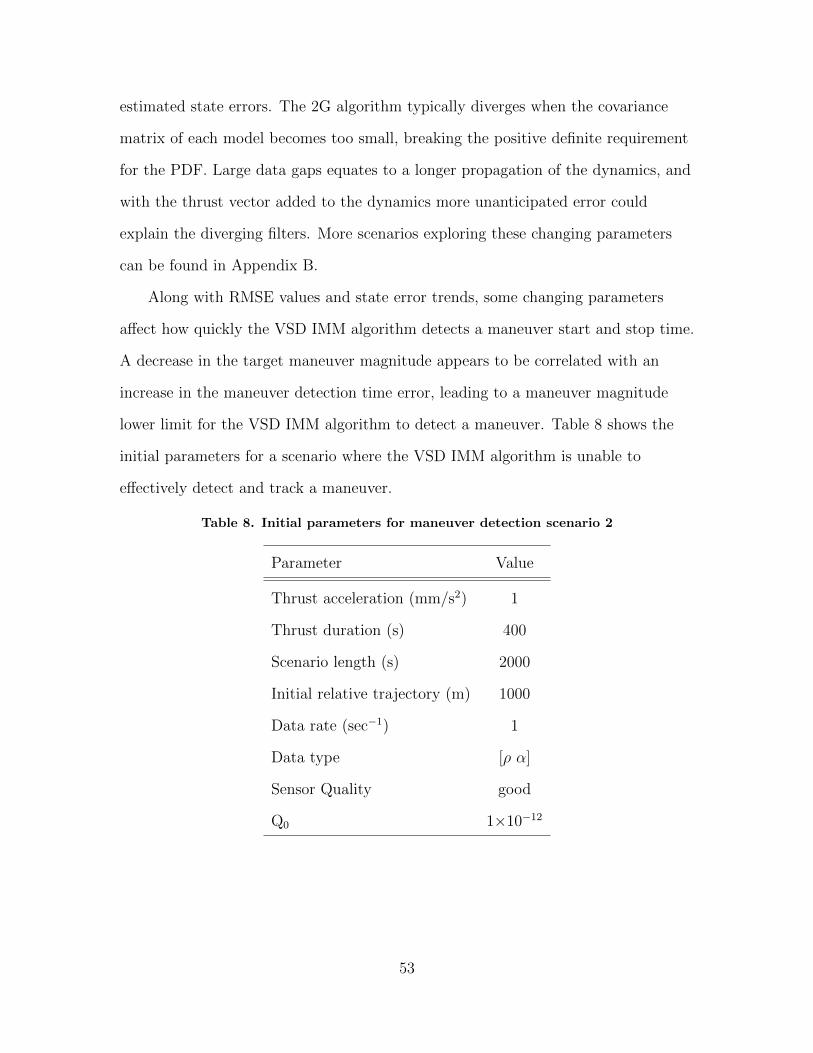
estimated state errors. The 2G algorithm typically diverges when the covariance
matrix of each model becomes too small, breaking the positive definite requirement
for the PDF. Large data gaps equates to a longer propagation of the dynamics, and
with the thrust vector added to the dynamics more unanticipated error could
explain the diverging filters. More scenarios exploring these changing parameters
can be found in Appendix B.
Along with RMSE values and state error trends, some changing parameters
affect how quickly the VSD IMM algorithm detects a maneuver start and stop time.
A decrease in the target maneuver magnitude appears to be correlated with an
increase in the maneuver detection time error, leading to a maneuver magnitude
lower limit for the VSD IMM algorithm to detect a maneuver. Table 8 shows the
initial parameters for a scenario where the VSD IMM algorithm is unable to
effectively detect and track a maneuver.
Table 8. Initial parameters for maneuver detection scenario 2
Parameter Value
Thrust acceleration (mm/s2) 1
Thrust duration (s) 400
Scenario length (s) 2000
Initial relative trajectory (m) 1000
Data rate (sec−1) 1
Data type [ρ α]
Sensor Quality good
Q0 1×10⁻¹²
53

As shown in Table 9, the RMSE values for each state remain relatively low in
this scenario, and the VSD IMM algorithm is able to detect the maneuver start
within seconds of error.
Table 9. Simulation results for maneuver detection scenario 2
RMSE IMM UKF
δx (m) 0.086
δy (m) 0.24
δx (m/s) 2.9×10⁻³
δy (m/s) 0.039
δT (m/s2) 8.22×10⁻⁴
Man start (s) 6.36
Man duration (s) 1.29×10³
However, the VSD IMM algorithm never detected a maneuver stop time,
estimating a maneuver magnitude long after the target stopped maneuvering. As
shown in Figure 7a, the maneuver detection statistic spikes around both the
maneuver start time and the maneuver stop time but never reaches the maneuver
detection threshold that signals the VSD to stop estimating a thrust vector.
However, continuously estimating the thrust vector post-maneuver does not seem to
affect the RMSE values of the scenario. Time plots show roughly a 10% increase in
error post maneuver but an overall recovery of the state error to baseline levels. As
shown in Figure 7b, the VSD filters continue to estimate a thrust vector
post-maneuver, capturing the small maneuver magnitude and reaching a zero steady
state thrust through the end of the scenario.
54

(a)
(b)
Figure 7. For maneuver detection scenario 2 (a) the maneuver detection statistic and(b) the thrust magnitude estimate vs truth
The second maneuver detection scenario opens a new level of investigation for
testing the performance of an IMM algorithm based on the claim that small target
maneuvers may not need to be detected in order to maintain baseline level state
errors.
55

4.2 Small Maneuver Analysis
The results from applying a 2G IMM algorithm to maneuver detection scenarios
show a possibility to handle small target maneuvers using an IMM framework
without the need for maneuver characterization. The following section analyzes a
small maneuver scenario using a 1G IMM algorithm without adding a thrust
acceleration vector to the system dynamics. The 1G IMM algorithm requires a level
of post processing that delays real-time analysis, but with the sensitivity of the VSD
filter and the PDF, a 1G IMM algorithm may be a more stable alternative given
varied scenario parameters. Table 10 shows the initial parameters for the first small
maneuver scenario using a 1G IMM algorithm.
Table 10. Initial parameters for small maneuver scenario 1
Parameter Value
Thrust acceleration (mm/s2) 1
Thrust duration (s) 400
Scenario length (s) 2000
Initial relative trajectory (m) 1000
Data rate (sec−1) 1
Data type [ρ α]
Sensor Quality good
Q0 1×10⁻⁸
Along with the UKF, the EKF is applied as a viable filter for these scenarios
because of the added stability of a constant dynamical model in the 1G IMM
algorithm. For the first scenario, an RMSE comparison does not show the difference
between a single filter and a series of IMM filters because the small maneuver does
not drastically change the dynamics from the baseline scenario. However, the
56
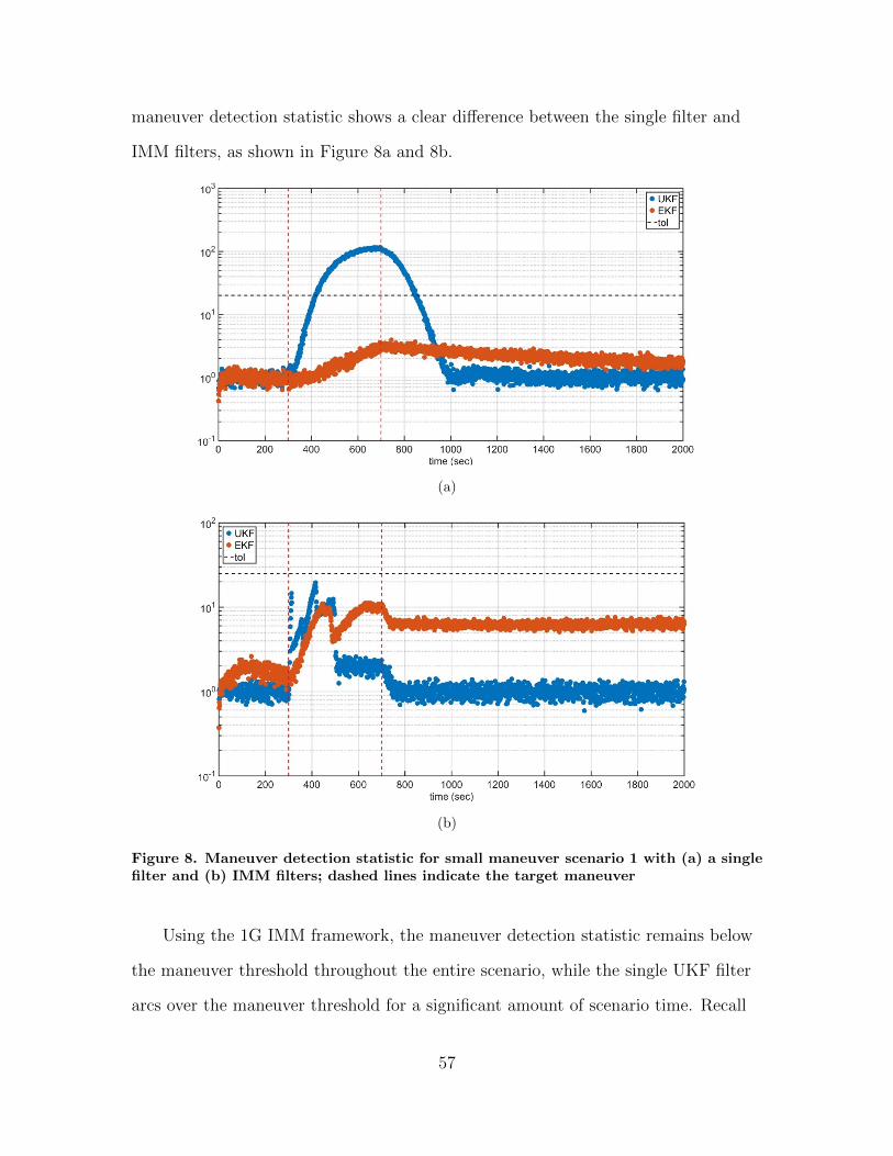
maneuver detection statistic shows a clear difference between the single filter and
IMM filters, as shown in Figure 8a and 8b.
(a)
(b)
Figure 8. Maneuver detection statistic for small maneuver scenario 1 with (a) a singlefilter and (b) IMM filters; dashed lines indicate the target maneuver
Using the 1G IMM framework, the maneuver detection statistic remains below
the maneuver threshold throughout the entire scenario, while the single UKF filter
arcs over the maneuver threshold for a significant amount of scenario time. Recall
57
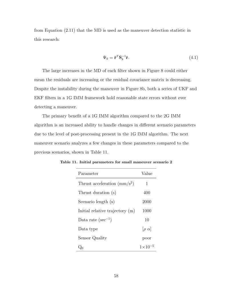
from Equation (2.11) that the MD is used as the maneuver detection statistic in
this research:
Ψk = rTS−1k r. (4.1)
The large increases in the MD of each filter shown in Figure 8 could either
mean the residuals are increasing or the residual covariance matrix is decreasing.
Despite the instability during the maneuver in Figure 8b, both a series of UKF and
EKF filters in a 1G IMM framework hold reasonable state errors without ever
detecting a maneuver.
The primary benefit of a 1G IMM algorithm compared to the 2G IMM
algorithm is an increased ability to handle changes in different scenario parameters
due to the level of post-processing present in the 1G IMM algorithm. The next
maneuver scenario analyzes a few changes in these parameters compared to the
previous scenarios, shown in Table 11.
Table 11. Initial parameters for small maneuver scenario 2
Parameter Value
Thrust acceleration (mm/s2) 1
Thrust duration (s) 400
Scenario length (s) 2000
Initial relative trajectory (m) 1000
Data rate (sec−1) 10
Data type [ρ α]
Sensor Quality poor
Q0 1×10⁻⁵
58

The second small maneuver scenario takes into account a slower data rate as
well as a poor sensor quality, causing a higher initial process noise covariance for
sufficient results. These worsening parameters appear to correlated with higher
RMSE values compared to the baseline scenario, as shown in Table 12. Since the
maneuver magnitude and duration is the same between the first and second small
maneuver scenarios, the worsening state errors do not appear to be correlated with
the small target maneuver.
Table 12. Simulation results for small maneuver scenario 2
RMSE Single UKF Single EKF IMM UKF IMM EKF
δx (m) 0.89 1.56 0.76 1.34
δy (m) 5.40 3.27 2.41 3.39
δx (m/s) 4.1×10⁻³ 7.1×10⁻³ 6.5×10⁻³ 9.3×10⁻³
δy (m/s) 0.071 0.23 0.046 0.24
The small maneuver scenarios serve as a validation of an alternative adaptive
estimation technique that does not involve the sensitive process of maneuver
detection. In scenarios where small target maneuvers are expected, adding an
adaptive estimation framework to relative orbit estimation allows an observer to
continue to track a maneuvering target without attempting to detect or characterize
the maneuver. However, the current study claims that maneuvers are well
characterized with improved state errors using adaptive estimation with the thrust
acceleration vector added as states to the system.
4.3 Maneuver Characterization Analysis
The 1G IMM algorithm is primarily utilized in this study as a means of
maneuver characterization. Compared to maneuver detection, maneuver
59

characterization focuses on capturing the target thrust acceleration vector and
analyzing the target maneuver in terms of magnitude and duration.
The first maneuver characterization scenario uses the exact same initial scenario
parameters as the first small maneuver scenario, shown in Table 10, but the filters
for this scenario are now permanently estimating a target maneuver as acceleration
states in both the radial and along-track directions. As shown in Table 13, both the
UKF and EKF filters in a 1G IMM framework have improved RMSE values
compared to the single UKF and EKF filters. The results using the 1G IMM
algorithm show that even in instances of small target maneuvers, estimating a thrust
acceleration for the entire scenario can accurately characterize a small maneuver
while maintaining lower state errors compared to not estimating a maneuver at all.
Table 13. Simulation results for maneuver characterization scenario 1
RMSE Single UKF Single EKF IMM UKF IMM EKF
δx (m) 0.89 1.56 0.11 0.41
δy (m) 5.40 3.27 0.24 0.84
δx (m/s) 4.1×10⁻³ 7.1×10⁻³ 4.9×10⁻³ 0.011
δy (m/s) 0.071 0.23 0.013 0.15
Tx (m/s2) 0.013 1.6e×10−5 1.1×10⁻⁴ 1.6×10⁻⁵
Ty (m/s2) 0.030 3.1e×10−3 4.7×10⁻⁴ 6.6×10⁻⁴
Along with keeping the state RMSE values at baseline levels, the 1G IMM
algorithm is highly efficient at characterizing maneuvers compared to single filter
estimators. As shown in Figure 9a, the small 1 mm/s2 maneuver is below the
inherent noise of the single UKF filter, and the single EKF filter converges quickly
to a steady state maneuver magnitude of zero. When these filters are applied to a
1G IMM framework as shown in Figure 9b, the UKF filters can now capture and
60

characterize the target maneuver, but the EKF filters have no way of quickly
adapting to the change in dynamics. Recall that the thrust acceleration vector is
assumed to be constant for both IMM algorithms, which can explain the delay in
tracking the maneuver for the UKF filters and the failure to characterize the
maneuver with EKF filters.
(a)
(b)
Figure 9. Thrust acceleration estimate for maneuver characterization scenario 1 with(a) a single filter and (b) IMM filters
61

The fact that the EKF filter cannot react quickly to a target maneuver causes
problems in maneuver characterization scenarios attempting to capture larger
maneuvers. The thrust magnitude for the second maneuver characterization scenario
is much larger, shown with the rest of the initial scenario parameters in Table 14.
Table 14. Initial parameters for maneuver characterization scenario 2
Parameter Value
Thrust acceleration (mm/s2) 100
Thrust duration (s) 400
Scenario length (s) 2000
Initial relative trajectory (m) 1000
Data rate (sec−1) 10
Data type [ρ ρ α]
Sensor Quality good
Q0 1×10⁻⁸
As seen in Table 15, using single UKFs and EKFs cause the state errors to
diverge dramatically, and neither filter can capture an accurate target maneuver
profile. These results drastically change when UKFs are used in an IMM framework,
but the EKFs are slow to adapt and cause the 1G IMM algorithm to diverge due to
a non-positive definite covariance matrix.
Despite the improvement of RMSE values from a single filter to a bank of IMM
filters, the IMM UKFs still do not reach error levels comparable to the baseline
scenario. This could be caused by the fact that the IMM algorithm continuously
estimates the thrust acceleration states long after the maneuver has stopped,
effectively contributing to the noise added to the estimator.
62
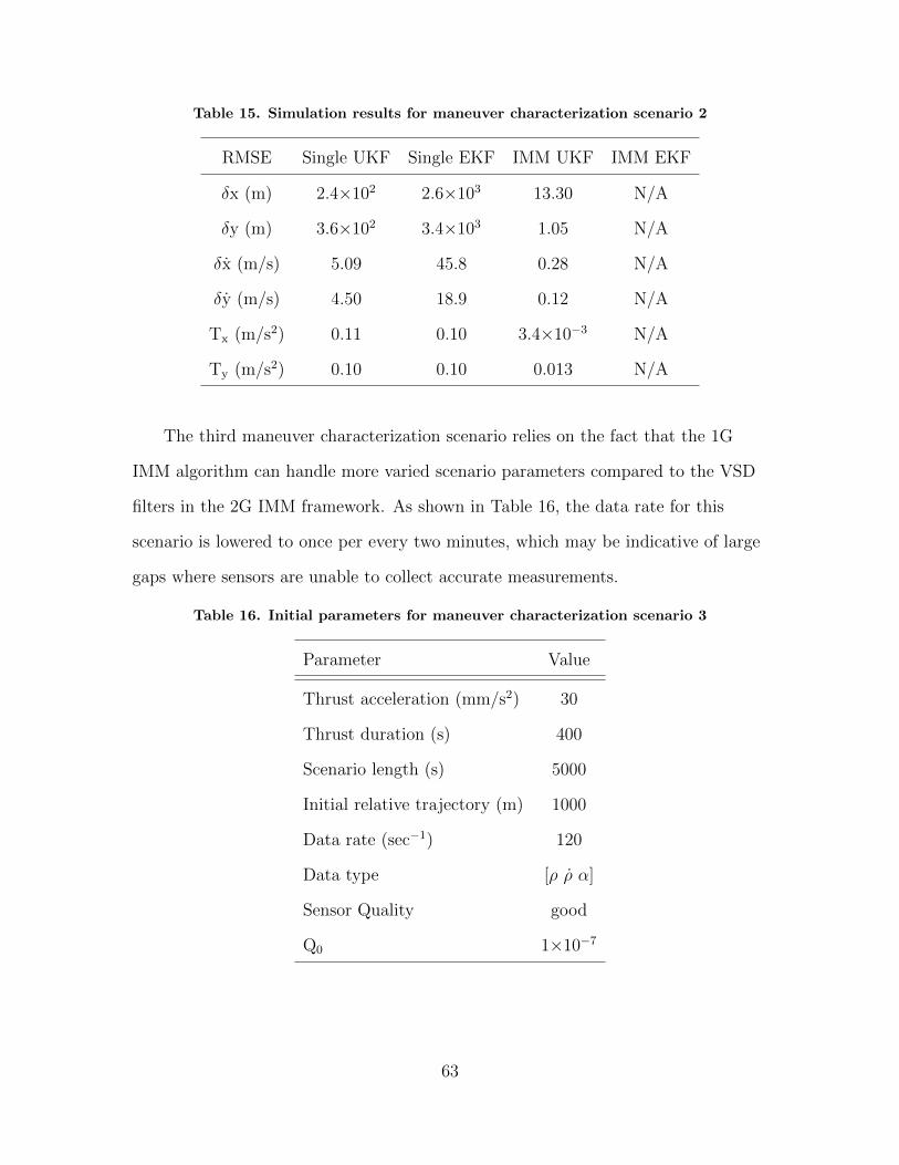
Table 15. Simulation results for maneuver characterization scenario 2
RMSE Single UKF Single EKF IMM UKF IMM EKF
δx (m) 2.4×10² 2.6×10³ 13.30 N/A
δy (m) 3.6×10² 3.4×10³ 1.05 N/A
δx (m/s) 5.09 45.8 0.28 N/A
δy (m/s) 4.50 18.9 0.12 N/A
Tx (m/s2) 0.11 0.10 3.4×10⁻³ N/A
Ty (m/s2) 0.10 0.10 0.013 N/A
The third maneuver characterization scenario relies on the fact that the 1G
IMM algorithm can handle more varied scenario parameters compared to the VSD
filters in the 2G IMM framework. As shown in Table 16, the data rate for this
scenario is lowered to once per every two minutes, which may be indicative of large
gaps where sensors are unable to collect accurate measurements.
Table 16. Initial parameters for maneuver characterization scenario 3
Parameter Value
Thrust acceleration (mm/s2) 30
Thrust duration (s) 400
Scenario length (s) 5000
Initial relative trajectory (m) 1000
Data rate (sec−1) 120
Data type [ρ ρ α]
Sensor Quality good
Q0 1×10⁻⁷
63
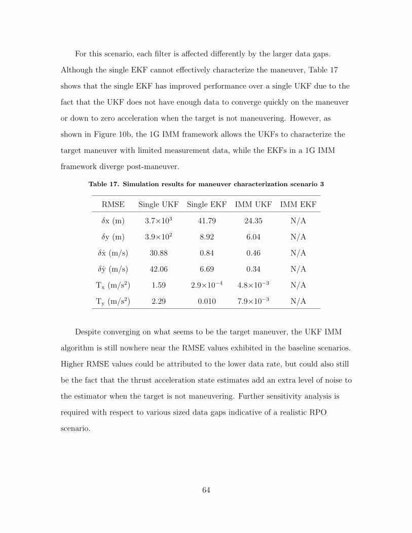
For this scenario, each filter is affected differently by the larger data gaps.
Although the single EKF cannot effectively characterize the maneuver, Table 17
shows that the single EKF has improved performance over a single UKF due to the
fact that the UKF does not have enough data to converge quickly on the maneuver
or down to zero acceleration when the target is not maneuvering. However, as
shown in Figure 10b, the 1G IMM framework allows the UKFs to characterize the
target maneuver with limited measurement data, while the EKFs in a 1G IMM
framework diverge post-maneuver.
Table 17. Simulation results for maneuver characterization scenario 3
RMSE Single UKF Single EKF IMM UKF IMM EKF
δx (m) 3.7×10³ 41.79 24.35 N/A
δy (m) 3.9×10² 8.92 6.04 N/A
δx (m/s) 30.88 0.84 0.46 N/A
δy (m/s) 42.06 6.69 0.34 N/A
Tx (m/s2) 1.59 2.9×10⁻⁴ 4.8×10⁻³ N/A
Ty (m/s2) 2.29 0.010 7.9×10⁻³ N/A
Despite converging on what seems to be the target maneuver, the UKF IMM
algorithm is still nowhere near the RMSE values exhibited in the baseline scenarios.
Higher RMSE values could be attributed to the lower data rate, but could also still
be the fact that the thrust acceleration state estimates add an extra level of noise to
the estimator when the target is not maneuvering. Further sensitivity analysis is
required with respect to various sized data gaps indicative of a realistic RPO
scenario.
64

(a)
(b)
Figure 10. Thrust acceleration estimate for maneuver characterization scenario 3 with(a) a single filter and (b) IMM filters
The maneuver characterization scenarios show the effectiveness of a band of
UKFs in a 1G IMM framework and their ability to characterize larger maneuvers
with limitations to data rate and sensor type, but the EKFs in an IMM framework
do not have enough inherent adaptability to characterize a maneuver effectively.
65

None of the maneuver characterization scenarios can attain RMSE values
comparable to the baseline scenario.
4.4 Dynamic Thrust Analysis
A major assumption used in this research is that the target is exhibiting a
constant thrust acceleration for the duration of the maneuver time. Although most
spacecraft are designed with propulsions systems that output a constant force, the
direction of that force and the subsequent acceleration of the target does not remain
constant. However,non-cooperative maneuvers are nearly impossible to accurately
predict in terms of both direction and magnitude without information about
propulsion capabilities of the target. This section addresses these realistic concerns
and attempts to solve them using the 1G IMM algorithm used in the previous
section.
The scenario presented in this section is an notional maneuver calculated by the
target in an attempt to rendezvous with the observer. The initial scenario
parameters are shown in Table 18.
66
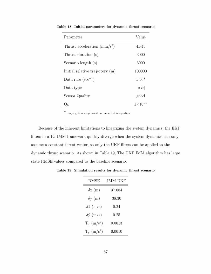
Table 18. Initial parameters for dynamic thrust scenario
Parameter Value
Thrust acceleration (mm/s2) 41-43
Thrust duration (s) 3000
Scenario length (s) 3000
Initial relative trajectory (m) 100000
Data rate (sec−1) 1-30*
Data type [ρ α]
Sensor Quality good
Q0 1×10⁻⁹
* varying time step based on numerical integration
Because of the inherent limitations to linearizing the system dynamics, the EKF
filters in a 1G IMM framework quickly diverge when the system dynamics can only
assume a constant thrust vector, so only the UKF filters can be applied to the
dynamic thrust scenario. As shown in Table 19, The UKF IMM algorithm has large
state RMSE values compared to the baseline scenario.
Table 19. Simulation results for dynamic thrust scenario
RMSE IMM UKF
δx (m) 37.084
δy (m) 38.30
δx (m/s) 0.24
δy (m/s) 0.25
Tx (m/s2) 0.0013
Ty (m/s2) 0.0010
67

Despite the target exhibiting a variable thrust vector and the estimator
dynamics assuming a constant thrust, the UKF IMM algorithm is able to track the
target maneuver throughout the scenario with approximately 1 mm/s2 worth of
error in each direction. Figure 11 shows the thrust acceleration estimates compared
to truth data in both the radial and along-track directions.
Figure 11. Thrust acceleration estimate for dynamic thrust scenario
The dynamic thrust scenario shows the adaptability of the 1G IMM algorithm
and its ability to handle drastic changes in not only the scenario parameters but
also the system dynamics. The 1G IMM algorithm is able to capture a relatively
accurate thrust acceleration vector for the target at the cost of high state errors
relative to the baseline scenario. Improvements to this algorithm can be made if
more information is known about the maneuver capabilities of the target spacecraft,
which could help estimate the dynamics of the thrust acceleration vector.
68

4.5 Parameter Study Conclusions
The current study uses five scenario parameters defined in Section 3.3.2 to
assess the performance of each adaptive estimation technique used to detect and
characterize non-cooperative maneuvers for RPO missions. Overall, the 2G IMM
algorithm has higher parameter requirements for convergence in terms of data rate
and data type, but both IMM algorithms have varying levels of success in terms of
maneuver detection and characterization when experiencing different scenario
parameters.
The most prominent parameter analyzed in this study is the target maneuver
magnitude. Both IMM algorithms are tested with both large and small relative
maneuvers with various results. Overall, the 2G IMM algorithm has more difficulty
detecting lower thrust magnitudes but maintains state errors consistent with the
baseline scenario. Higher thrust magnitudes appear to be correlated with higher
state errors but lower errors in maneuver detection times. The 1G IMM algorithm
can effectively characterize maneuvers of various thrust magnitudes, but at the cost
of higher state errors than the baseline scenario, especially when other scenario
parameters vary.
Decreasing the observer sensor accuracy is most directly correlated with higher
state errors for both IMM algorithms, but does not immediately cause convergence
issues. As seen in Table 11 and other scenarios with poor sensor accuracy in
Appendix B, a worsening sensor accuracy is also correlated with a higher process
noise covariance, which conceptually refers to the fact that the estimator has a lower
confidence in the system dynamics when it is fed less accurate measurements.
The scenario in Section 4.4 first analyzes changes in relative trajectory of the
target. Due to the variable levels of process noise allowed by adaptive estimation,
the relative trajectory assumption used in the HCW dynamical equations becomes
69

invalid before the IMM algorithms fail to converge. Initial analysis of the relative
trajectory parameter shows successful scenarios using UKF filters in an IMM
framework and nonlinear relative equations of motion. An EKF IMM algorithm
using similar dynamics runs into significant issues regarding computation time due
to the linearization process necessary in the EKF framework. Further analysis of
the IMM algorithms with nonlinear dynamics is shown in Appendix C.
Changes in the data rate parameter can cause significantly higher state errors as
well as convergence issues for both IMM algorithms. Any collection rate longer than
1 Hz appears to cause the 2G IMM algorithm to diverge. The 1G IMM algorithm
can handle longer gaps between measurements, as seen in Figure 10, but can still
experience significantly higher state errors. Conceptually speaking, higher state
errors could cause a limit in data type as well if a sensor loses its pointing accuracy
on the target.
The data type is the most difficult parameter to change due to significant
convergence issues for both IMM algorithms. In this study, the 2G IMM algorithm
cannot converge on an accurate maneuver estimate without any other data type
besides range and azimuth data. The 1G IMM algorithm can also handle range rate
measurements, but as seen in Table 15 there is no significant benefit to the state
error by adding this extra measurement. Any limited measurement scenario
(range/range rate or angles-only data types) causes a drastic increase in state errors
and is not feasible for the applications of adaptive estimation in the current study.
4.6 IMM Algorithm Analysis
The initial analysis of the current study does not focus on the structure of
adaptive estimation techniques, but there are observed differences in how the 1G
and 2G IMM algorithms calculate the weights for each filter model. As shown in
70

Figure 12a, only one model dominates the estimation at a time in the 1G IMM
algorithm, and significant model switching only takes place while the target is
maneuvering. For the 2G IMM algorithm shown in Figure 12b, the model weights
are only calculated when the VSD filters are active, and because of the real-time
nature of the algorithm there is a significant amount of active interaction between
each model.
(a)
(b)
Figure 12. Typical model weights for (a) a 1G IMM algorithm and (b) a 2G IMMalgorithm; dashed lines indicate the target maneuver
71

Further analysis of the maneuver detection scenarios imply that increased
model interaction could be correlated with increasing state errors in the models.
Figure 13 shows the model weights for maneuver detection scenarios 3 and 4, results
of which can be found in Appendix B. Maneuver detection scenario 3 has low state
errors and accurate detection times for the VSD filter, which appears to be
correlated with the IMM algorithm converging on a single model, as seen in Figure
13a. Maneuver detection scenario 4 uses poor sensors, which cause higher state
errors and a larger error in maneuver detection times. As seen in Figure 13b, the
target maneuver stops at 700 seconds, and the small amount of time post-maneuver
with the VSD still on sees the most sporadic model interactions. Within the scope
of the scenarios analyzed in this study, large deviations between the predicted and
the truth dynamical models seem to correlate with more dynamic model
interactions to handle the increasing state errors.
Figures 12 and 13 show and initial analysis for the dynamics behind model
interactions, but without a clear pattern across all scenarios there is no clear
method to predict how the model weights will interact or which model will
dominate over the others. Distributing the process noise covariance at an order of
magnitude over 5 separate models is taken from [7] without any further analysis due
to the similar applications of the adaptive estimation algorithms, but further
analysis into the number of models and the distribution of the model hypotheses is
beyond the scope of this research. Future work concerning the extended analysis of
adaptive estimation is outlined in Section 5.3.
72
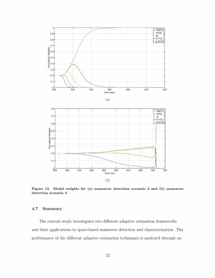
(a)
(b)
Figure 13. Model weights for (a) maneuver detection scenario 3 and (b) maneuverdetection scenario 4
4.7 Summary
The current study investigates two different adaptive estimation frameworks
and their applications to space-based maneuver detection and characterization. The
performance of the different adaptive estimation techniques is analyzed through an
73

extensive parameter study focused on the efficacy of maneuver characterization and
state error comparison to non-maneuvering scenarios. The research analysis
concludes that a 2G IMM algorithm with VSD filters is reliant on more stringent
parameter requirements for convergence, while a 1G IMM algorithm experiences a
higher adaptability to changing parameters at the cost of inherently higher state
errors. Further research and analysis is required to make conclusions on the
dynamical aspects of the IMM algorithms, and entirely new algorithms may be
required for optimal performance regarding adaptive estimation.
74
V. Conclusions and Recommendations
The goals of this study were to investigate adaptive estimation techniques and
their applications to space-based maneuver detection and characterization for RPO
missions. Overall, the research showed that adaptive estimation algorithms
outperform single KF algorithms at detecting and characterizing non-cooperative
maneuvers while maintaining similar state errors compared to tracking
non-maneuvering targets. The following chapter reviews the research questions
answered in this study, the motivation and scope of this study, and concludes with
recommendations for future work on this topic.
5.1 Research Questions Answered
The current study was divided into three relevant research questions designed to
explore current adaptive estimation techniques and their applications to RPO
through an in-depth parameter study and convergence analysis. The following
research questions were answered in this study:
• Can adaptive estimation techniques be applied to detect and characterize
non-cooperative spacecraft maneuvers in satellite close proximity operations?
– Section 4.1 shows that a 2G IMM algorithm coupled with VSD filters can
detect non-cooperative maneuvers using relative spacecraft dynamics and
measurements. Every successful scenario is able to accurately characterize
the target maneuver within 1 mm/s2 of error, all while maintaining state
errors comparable to a non-maneuvering scenario. However, varying
scenario parameters reveal the sensitivity of the algorithm.
75
• How do sensor source and type, data rate, maneuver magnitudes, and relative
trajectory affect the performance of an adaptive estimation algorithm?
– Section 4.5 outlines how different scenario parameters appear to be
correlated to the performance of both the 1G and 2G IMM algorithms.
Overall, the 1G IMM algorithm is able to handle more parameter changes
than the 2G IMM algorithm due to the sensitivity of the VSD filters with
the PDF, but the 2G IMM algorithm has lower state errors when working
properly.
• For what types of scenarios does an adaptive estimation algorithm fail to
detect a maneuver or fail to characterize an accurate maneuver magnitude?
– In relation to the current study, the adaptive estimation algorithm fails
to converge in instances of large measurement gaps, large target
maneuver magnitudes, and limited types of measurements. The 2G IMM
algorithm is especially sensitive to covariance inflation and initial
conditions for the VSD filters. Further analysis in Section 4.2 of this
research shows that small maneuvers unable to be detected by a 2G IMM
algorithm can still be characterized by a 1G IMM algorithm at the cost
of higher state errors.
5.2 Research Implications
The motivation behind this research is to aid in the assessment of orbital
estimation algorithms with the potential for future use by the USAF to protect
space assets through improved SSA. The algorithms demonstrated in this research
contributed to the state-of-the-art in orbital estimation by applying maneuver
detection and characterization to space-based scenarios. In combination with its
76
dedicated set of ground-based sensors, the JSpOC can utilize space-based SSA to
enhance its space object tracking and lower the chances of creating a UCT due to
non-cooperative maneuvers and sensor limitations. Correlating the assessment of
adaptive estimation techniques with space-based sensors also aids the USAF space
acquisition community in designing better space assets focused on the SSA mission.
The scope of this research focused on space-based applications of adaptive
estimation to detect and characterize non-cooperative maneuvers of a target
spacecraft in RPO. The current study assumed that the target spacecraft is
conducting a continuous, low-thrust maneuver designed to maintain its RPO
mission; that initial orbit determination (IOD) of the target has been acquired,
which gives the observer adequate information regarding the initial states of the
target; and that the target is exhibiting in-plane motion around the observer,
further simplifying the problem in order to focus on analyzing the estimation
techniques themselves.
This research makes no conclusions on the reason behind any dynamic
interaction between the models in each maneuvering scenario, and no optimization
scheme was attempted to further improve the adaptive estimation algorithms. The
conclusion can simply be made that dynamic, real-time maneuver detection and
characterization is further improved in both responsiveness and accuracy by using
adaptive estimation. Within the scope of this topic and the assumptions made for
this study, the research shows that adaptive estimation techniques can be a viable
option for future non-cooperative scenarios where full dynamical knowledge of the
target spacecraft is not available.
77
5.3 Potential Future Research
There are multiple topics and concepts covered in this study that could benefit
from further application. A more general RPO scenario requires a full application of
three-dimensional nonlinear motion of the target spacecraft relative to the observer.
The nonlinear relative satellite motion dynamics are able to more accurately model
scenarios without proximity requirements as well as an observer in an elliptical
orbit. A full operational application of this research also requires IOD of the target
spacecraft and combining space-based with supplemental ground based sensor data,
further improving SSA on the target.
Although the current study made viable conclusions on the performance of
adaptive estimation techniques for maneuver detection and characterization, the
scope of this research barely skimmed the surface on adaptive estimation theory.
How and why each model interacts with other models before, during, and after a
maneuver requires further investigation which could lead to a better range of
dynamic hypotheses for each model. Each IMM algorithm applied in this study also
had a fixed number of models with preallocated hypotheses on the dynamics of the
system. Further analysis is required to assess how changing the number of models
and the range of hypotheses affects performance and responsiveness. Lastly, the
IMM algorithms in this study made hypotheses solely on the process noise
covariance applied to the system dynamics, but the IMM framework can be
designed to make any number of hypotheses based on the uncertainty of the
maneuvering target. Useful future applications of the IMM algorithm may involve
assessing different ranges of sensor noise or even making guesses at the thrust vector
of the target.
Another area of potential future work involves applying adaptive estimation to
a variety of different target maneuvers that represent more realistic RPO missions.
78
Section 4.4 assesses the performance of the 1G IMM algorithm with a dynamic
thrust vector, but the estimator still assumes that the maneuver states remain
constant throughout the scenario. Although most space-based thrusters exhibit a
constant force, the perceived acceleration of the target relative to the observer
changes with respect to the propellant burned by the target. The dynamic thrust
scenarios showed that adaptive estimation techniques may not be sufficient if the
thrust vector is assumed to be constant, so information must be fed into the filter
that allows the estimation technique to predict the maneuver magnitude with
respect to the assumed mass of the target spacecraft.
Along with the assumptions regarding the maneuver magnitude, the adaptive
estimation techniques demonstrated in this research requires further study into
other realistic RPO missions. This study simply applied a constant maneuver for a
predetermined period of time to the target without any mission goals in mind. A
more realistic maneuver detection scenario takes into account a certain mission
objective for both the target and the observer as well as gaps in measurement data
where sensors are blocked by the Sun vector or in eclipse.
5.4 Conclusion
The research demonstrated herein investigates different adaptive estimation
techniques and their applications in non-cooperative maneuver detection and
characterization of target spacecraft operating in close proximity to an observer
spacecraft. Adaptive estimation utilizes a bank of filters with different hypotheses
on a system’s dynamics to account for unexpected changes in the dynamical model.
Combined with a series of VSD filters, the adaptive estimation algorithm is able to
detect and track target maneuvers of reasonable magnitude given a high rate of
measurement data. A more classical adaptive estimation approach is able to
79

characterize maneuvers with a wider variety of changing scenario parameters at the
cost of a small increase in estimated state errors. Overall, adaptive estimation is a
vast area of research with a variety of useful applications to the space-based SSA
mission of the USAF.
80

Appendix A. Estimation Algorithms
Algorithm 1: Extended Kalman Filter
1 Initialize or define previous state and covariance: x0, P0 or xi−1, Pi−1
2 Propagate state from ti−1 to ti to determine xi and Φ(ti, ti−1)
Initial condition: xi−1 Differential eq: x = f(x, t)
Initial condition: Φ(ti−1, ti−1) = I Differential eq: Φ = ∂f(x,t)∂x
Φ(ti, ti−1)
3 Update covariance:
Pi = Φ(ti, ti−1)Pi−1Φ(ti, ti−1)T + Qi
4 Read in observation and sensor noise at ti: yi, Ri
5 Calculate the measurement basis function and residuals:
Hi = ∂G(xi,t)∂x
νi = yi −G(xi, ti)
6 Calculate the observation covariance and mahalanobis distance:
Si = HiPiHTi + Ri Ψi = νTi S−1
i νi
7 Use the Kalman gain to correct the updated state and covariance:
Ki = PiHTi S−1
i xi = xi + Kiνi Pi = (I−KiHi) Pi
8 Return to step 1, process observation at ti+1
81
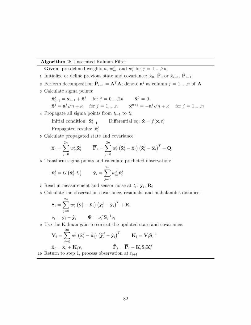
Algorithm 2: Unscented Kalman Filter
Given: pre-defined weights κ, wjm, and wjc for j = 1,...,2n
1 Initialize or define previous state and covariance: x0, P0 or xi−1, Pi−1
2 Perform decomposition Pi−1 = ATA; denote aj as column j = 1,...,n of A
3 Calculate sigma points:
xji−1 = xi−1 + xj for j = 0,...,2n x0 = 0
xj = aj√n+ κ for j = 1,...,n xn+j = −aj
√n+ κ for j = 1,...,n
4 Propagate all sigma points from ti−1 to ti:
Initial condition: xji−1 Differential eq: x = f(x, t)
Propagated results: xji5 Calculate propagated state and covariance:
xi =2n∑j=0
wjmxji Pi =2n∑j=0
wjc(xji − xi
) (xji − xi
)T+ Qi
6 Transform sigma points and calculate predicted observation:
yji = G(xji , ti
)yi =
2n∑j=0
wjmyji
7 Read in measurement and sensor noise at t i: yi, Ri
8 Calculate the observation covariance, residuals, and mahalanobis distance:
Si =2n∑j=0
wjc(yji − yi
) (yji − yi
)T+ Ri
νi = yi − yi Ψ = νTi S−1i νi
9 Use the Kalman gain to correct the updated state and covariance:
Vi =2n∑j=0
wjc(xji − xi
) (yji − yi
)TKi = ViS
−1i
xi = xi + Kivi Pi = Pi −KiSiKTi
10 Return to step 1, process observation at ti+1
82

Algorithm 3: Interacting Multiple Model
1 Determine mixing probabilities at time of next observation, t i:
ck =N∑j=1
Prj|kwji−1 for each model k up to N models
wj|ki−1 = 1
ckPrj|kw
ji−1 for all N 2 model combinations
2 Determine the individual state and covariance for each model k :
xki−1 =N∑j=1
xji−1wj|ki−1
Pki−1 =
N∑j=1
wj|ki−1
[Pji−1 +
(xji−1 − xki−1
) (xji−1 − xki−1
)T]3 Input xki−1 and Pk
i−1 into each filter k, propagate and update the estimatedstate, covariance, residual, and observation covariance through eachindividual model: xki , Pk
i , νki , and Ski .
4 Update the likelihood change and updated weight for each model using theprobability density function:
Λki = N
(νki ; 0,Ski
)= 1√
|2πSki |e
−12 (νki )
T(Sk
i )−1νki wki =
Λki ck
N∑j=1
Λjicj
5 Calculate weighted estimates:
xi =N∑k=1
xkiwki Ψi =
N∑k=1
wki Ψ
ki
Pi =N∑k=1
wki
[Pki +
(xki − xi
) (xki − xi
)T]6 Return to step 1, process observation at t i+1
83

Appendix B. Additional Scenarios and Results
In stochastic estimation, there is a trade off between not having enough data for
statistical relevance and having too much data that distracts from the claims made
by the research. The following results are additional scenarios that emphasize the
claims made in Chapter 4 without inflating the main body of the work.
Maneuver detection scenarios 3 and 4 show successful detections of average
target maneuver magnitudes. Maneuver detection scenario 4 shows that the 2G
IMM algorithm still works given poor sensor measurements with an inflated initial
process noise covariance.
Table 20. Initial parameters for maneuver detection scenario 3
Parameter Value
Thrust acceleration (mm/s2) 10
Thrust duration (s) 100
Scenario length (s) 1500
Initial relative trajectory (m) 1000
Data rate (sec−1) 1
Data type [ρ α]
Sensor Quality good
Q0 1×10⁻¹⁰
84

Table 21. Simulation results for maneuver detection scenario 3
RMSE IMM UKF
δx (m) 0.035
δy (m) 0.16
δx (m/s) 2.0×10⁻³
δy (m/s) 0.048
δT (m/s2) 2.99×10⁻³
Man start (s) 2.86
Man duration (s) 0.87
Table 22. Initial parameters for maneuver detection scenario 4
Parameter Value
Thrust acceleration (mm/s2) 50
Thrust duration (s) 400
Scenario length (s) 1500
Initial relative trajectory (m) 1000
Data rate (sec−1) 1
Data type [ρ α]
Sensor Quality poor
Q0 1×10⁻⁵
85

Table 23. Simulation results for maneuver detection scenario 4
RMSE IMM UKF
δx (m) 1.09
δy (m) 0.44
δx (m/s) 0.070
δy (m/s) 0.10
δT (m/s2) 8.62×10⁻⁴
Man start (s) 13.83
Man duration (s) 3.45
Small maneuver scenario 1 has no significant difference in error between the
single filter and IMM filters.
Table 24. Simulation results for small maneuver scenario 1
RMSE Single UKF Single EKF IMM UKF IMM EKF
δx (m) 0.56 0.36 0.098 0.64
δy (m) 3.45 0.75 0.76 1.42
δx (m/s) 8.6×10⁻³ 0.061 2.9×10⁻³ 0.064
δy (m/s) 0.056 0.27 0.026 0.28
Maneuver characterization scenario 4 has a harder time characterizing a large
maneuver with poor sensors, but RMSE values are along the same lines as other
scenarios with poor sensors.
86

Table 25. Initial parameters for maneuver characterization scenario 4
Parameter Value
Thrust acceleration (mm/s2) 100
Thrust duration (s) 100
Scenario length (s) 1500
Initial relative trajectory (m) 1000
Data rate (sec−1) 10
Data type [ρ α]
Sensor Quality poor
Q0 1×10⁻⁷
Table 26. Simulation results for maneuver characterization scenario 4
RMSE Single UKF Single EKF IMM UKF IMM EKF
δx (m) 11.70 25.56 4.03 9.60
δy (m) 21.74 3.47 2.17 6.27
δx (m/s) 0.20 0.14 0.087 2.37
δy (m/s) 1.08 3.52 0.34 1.68
Tx (m/s2) 2.0×10⁻³ 3.6×10⁻⁴ 1.6×10⁻³ 6.0×10⁻³
Ty (m/s2) 0.30 0.028 0.022 0.027
Two more dynamic thrust scenarios show similar RMSE values and maneuver
characterization success.
87

Table 27. Simulation results for dynamic thrust scenario 2
RMSE IMM UKF
δx (m) 46.70
δy (m) 45.58
δx (m/s) 0.31
δy (m/s) 0.32
Tx (m/s2) 0.0016
Ty (m/s2) 0.0024
Table 28. Simulation results for dynamic thrust scenario 3
RMSE IMM UKF
δx (m) 39.14
δy (m) 41.78
δx (m/s) 0.25
δy (m/s) 0.27
Tx (m/s2) 0.0012
Ty (m/s2) 0.0011
88

Appendix C. Nonlinear Dynamical Analysis
Based on preliminary analysis, Section 4.5 claims that the relative trajectory
assumption for the HCW equations of motion becomes invalid before the adaptive
estimation algorithm diverges. The relative trajectory parameter is not a primary
focus in this study because a large distance between the observer and the target
degrades the analysis for this study with respect to RPO scenarios.
The following scenario has the same initial conditions and uses a 2G IMM
algorithm for maneuver detection, but one IMM algorithm propagates the state
vector using the linearized HCW equations of motion (Equation (2.15)), while the
other IMM algorithm propagates the state vector using the nonlinear HCW
equations of motion without the relative trajectory assumption (Equation (2.17)).
Table 29 shows the initial conditions for the scenario, while Table 30 shows the
results for the scenario.
Table 29. Initial parameters for the relative trajectory scenario
Parameter Value
Thrust acceleration (mm/s2) 30
Thrust duration (s) 100
Scenario length (s) 1500
Initial relative trajectory (m) 1.0×10⁵
Data rate (sec−1) 1
Data type [ρ α]
Sensor Quality good
Q0 1×10⁻¹²
Based on results in Table 30, the dynamics appear to worsen the estimated
state vector, but the 2G IMM algorithm still detects a maneuver with seconds of
89

error. The higher RMSE values could be attributed to the large relative trajectory,
which adds noise to the range measurements themselves, or the degraded dynamics
at large relative trajectories, which seems counter intuitive for this scenario because
the nonlinear dynamics produce higher RMSE values than the linear dynamics.
Table 30. Simulation results for the relative trajectory scenario
RMSE Linear IMM UKF Nonlinear IMM UKF
δx (m) 7.08 44.24
δy (m) 43.89 326.22
δx (m/s) 0.039 0.12
δy (m/s) 0.57 1.16
Man start (s) 0.99 0.99
Man duration (s) 1.33 4.71
90

Bibliography
[1] B. J. Weichert, “The High Ground: The Case for U.S. Space Dominance,”Orbis, vol. 61, no. 2, pp. 227–237, 2017.
[2] National Research Council, Continuing Kepler’s Quest Assessing Air ForceSpace Command’s Astrodynamics Standards. The National Academies Press,2012.
[3] Department of Defense & Office of the Director of National Intelligence,National Security Space Strategy Unclassified Summary. 2011.
[4] United Nations General Assembly, “Report of the Committe on the PeacefulUses of Outer Space,” 1975.
[5] M. Wasson, “Space Situational Awareness in the Joint Space OperationsCenter,” Advanced Maui Optical and Space Surveillance Conference, vol. 298,no. 0704, pp. 8–10, 2011.
[6] M. A. Baird, “Maintaining Space Situational Awareness and Taking it to theNext Level,” Air and Space Power Journal, vol. 27, no. 5, pp. 50–72, 2013.
[7] G. M. Goff, Orbit Estimation of Non-Cooperative Maneuvering Spacecraft. PhDthesis, Air Force Institute of Technology, 2015.
[8] G. M. Goff, J. T. Black, and J. A. Beck, “Orbit Estimation of a ContinuouslyThrusting Spacecraft Using Variable Dimension Filters,” Journal of Guidance,Control, and Dynamics, vol. 38, no. 12, pp. 2407–2420, 2015.
[9] W. E. Wiesel, Modern Orbit Determination. Beavercreek, Ohio: AphelionPress, 2nd ed., 2010.
[10] C. F. Gauss, Theory of the Motion of the Heavenly Bodies Moving about theSun in Conic Sections. Mieola, NY: Dover Publications, 1857.
[11] B. D. Tapley, B. E. Schutz, and G. H. G. H. Born, Statistical OrbitDetermination. Burlington, MA: Elsevier Academic Press, 1st ed., 2004.
[12] R. F. Stengel, Optimal Control and Estimation. New York, NY: DoverPublications, 1994.
[13] U. P. Desai, A Comparative Study of Estimation Models for Satellite RelativeMotion. PhD thesis, Texas A&M University, 2013.
[14] H. W. Sorenson, “Least-squares estimation: from Gauss to Kalman,” IEEESpectrum, vol. 7, no. 7, pp. 63–68, 1970.
91
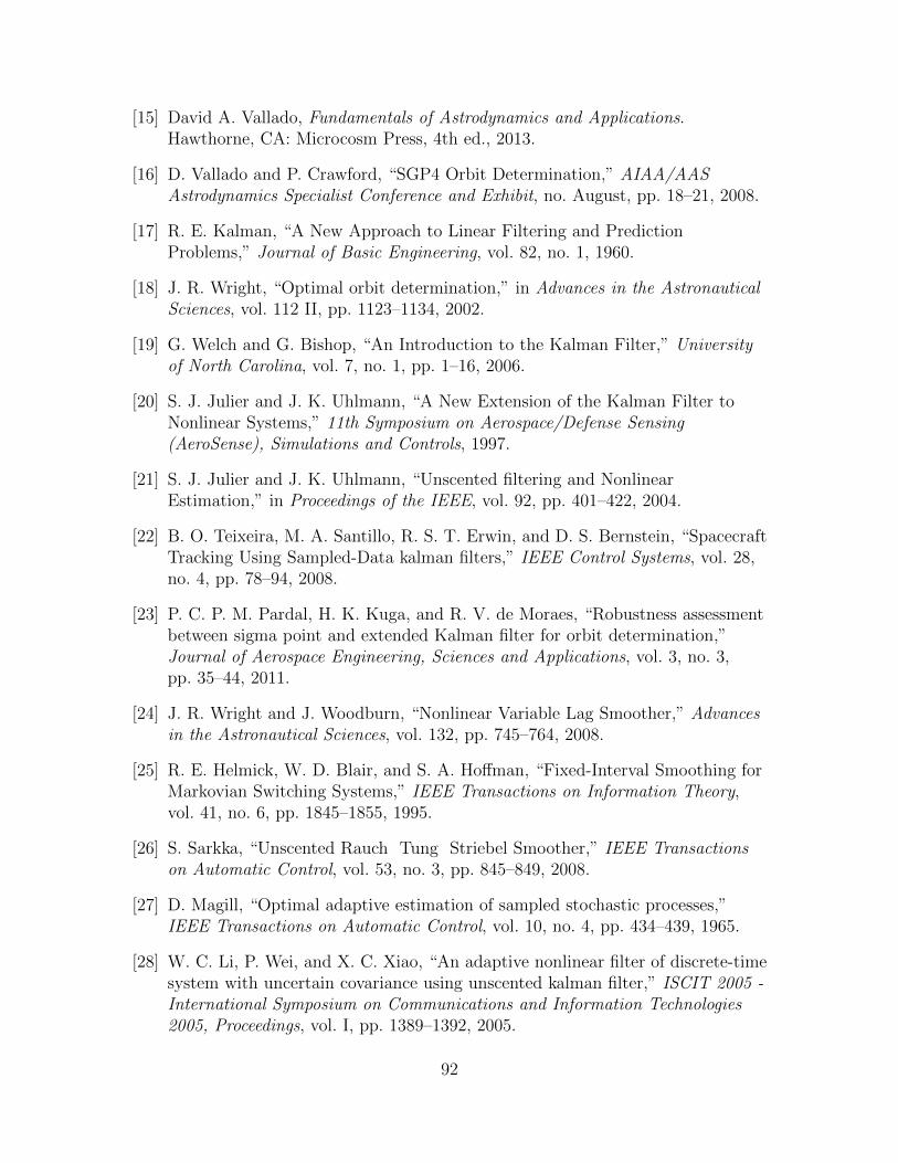
[15] David A. Vallado, Fundamentals of Astrodynamics and Applications.Hawthorne, CA: Microcosm Press, 4th ed., 2013.
[16] D. Vallado and P. Crawford, “SGP4 Orbit Determination,” AIAA/AASAstrodynamics Specialist Conference and Exhibit, no. August, pp. 18–21, 2008.
[17] R. E. Kalman, “A New Approach to Linear Filtering and PredictionProblems,” Journal of Basic Engineering, vol. 82, no. 1, 1960.
[18] J. R. Wright, “Optimal orbit determination,” in Advances in the AstronauticalSciences, vol. 112 II, pp. 1123–1134, 2002.
[19] G. Welch and G. Bishop, “An Introduction to the Kalman Filter,” Universityof North Carolina, vol. 7, no. 1, pp. 1–16, 2006.
[20] S. J. Julier and J. K. Uhlmann, “A New Extension of the Kalman Filter toNonlinear Systems,” 11th Symposium on Aerospace/Defense Sensing(AeroSense), Simulations and Controls, 1997.
[21] S. J. Julier and J. K. Uhlmann, “Unscented filtering and NonlinearEstimation,” in Proceedings of the IEEE, vol. 92, pp. 401–422, 2004.
[22] B. O. Teixeira, M. A. Santillo, R. S. T. Erwin, and D. S. Bernstein, “SpacecraftTracking Using Sampled-Data kalman filters,” IEEE Control Systems, vol. 28,no. 4, pp. 78–94, 2008.
[23] P. C. P. M. Pardal, H. K. Kuga, and R. V. de Moraes, “Robustness assessmentbetween sigma point and extended Kalman filter for orbit determination,”Journal of Aerospace Engineering, Sciences and Applications, vol. 3, no. 3,pp. 35–44, 2011.
[24] J. R. Wright and J. Woodburn, “Nonlinear Variable Lag Smoother,” Advancesin the Astronautical Sciences, vol. 132, pp. 745–764, 2008.
[25] R. E. Helmick, W. D. Blair, and S. A. Hoffman, “Fixed-Interval Smoothing forMarkovian Switching Systems,” IEEE Transactions on Information Theory,vol. 41, no. 6, pp. 1845–1855, 1995.
[26] S. Sarkka, “Unscented Rauch Tung Striebel Smoother,” IEEE Transactionson Automatic Control, vol. 53, no. 3, pp. 845–849, 2008.
[27] D. Magill, “Optimal adaptive estimation of sampled stochastic processes,”IEEE Transactions on Automatic Control, vol. 10, no. 4, pp. 434–439, 1965.
[28] W. C. Li, P. Wei, and X. C. Xiao, “An adaptive nonlinear filter of discrete-timesystem with uncertain covariance using unscented kalman filter,” ISCIT 2005 -International Symposium on Communications and Information Technologies2005, Proceedings, vol. I, pp. 1389–1392, 2005.
92

[29] R. L. Moose, “An Adaptive State Estimation Solution to the ManeuveringTarget Problem,” IEEE Transactions on Automatic Control, vol. 20, no. 3,pp. 359–362, 1975.
[30] X. R. Li and V. P. Jilkov, “Survey of Maneuvering Target Tracking. Part V:Multiple-Model Methods,” IEEE Transactions on Aerospace and ElectronicSystems, vol. 41, no. 4, pp. 1255–1321, 2005.
[31] D. A. Vallado and J. H. Seago, “Covariance Realism,” in AAS/AIAAAstrodynamics Specialist Conference, (Pittsburgh, PA), pp. 1–19, 2009.
[32] H. A. P. Blom and Y. Bar-Shalom, “The Interacting Multiple Model Algorithmfor Systems with Markovian Switching Coefficients,” IEEE Transactions onAutomatic Control, vol. 33, no. 8, pp. 780–783, 1988.
[33] Y. Bar-Shalom and K. Birmiwal, “Variable Dimension Filter for ManeuveringTarget Tracking,” IEEE Transactions on Aerospace and Electronic Systems,vol. AES-18, no. 5, pp. 621–629, 1982.
[34] T. K. Yaakov Bar-Shalom, X. Rong LI, Estimation with Applications toTracking and Navigation. New York, NY: John Wiley & Sons, Inc., 2001.
[35] R. De Maesschalck, D. Jouan-Rimbaud, and D. L. Massart, “The Mahalanobisdistance,” Chemometrics and Intelligent Laboratory Systems, vol. 50, no. 1,pp. 1–18, 2000.
[36] G. W. Hill, “Researches in the Lunar Theory,” American Journal ofMathematics, vol. 1, no. 1, 1878.
[37] W. H. Clohessy and R. S. Wiltshire, “Terminal Guidance System for SatelliteRendezvous,” Journal of the Aerospace Sciences, vol. 27, no. 9, pp. 653–658,1960.
[38] W. E. Wiesel, Spaceflight Dynamics. Beavercreek, Ohio: Aphelion Press,3rd ed., 2010.
[39] R. Bate, D. Mueller, and J. White, Fundamentals of Astrodynamics. 1971.
[40] T. A. Lovell and S. Tragesser, “Guidance for Relative Motion of Low EarthOrbit Spacecraft Based on Relative Orbit Elements,” AIAA/AASAstrodynamics Specialist Conference and Exhibit, no. August, pp. 1–16, 2004.
[41] C. Doolittle, F. Chavez, and T. A. Lovell, “Relative Orbit Element Estimationfor Satellite Navigation,” AIAA Guidance, Navigation, and Control Conferenceand Exhibition, no. August, pp. 1–11, 2005.
[42] P. R. Escobal, Methods of Orbit Determination. New York, NY: J. Wiley, 1965.
93

[43] G. Gaias, S. D’Amico, and J.-S. Ardaens, “Angles-Only Navigation to aNoncooperative Satellite Using Relative Orbital Elements,” Journal ofGuidance, Control, and Dynamics, vol. 37, no. 2, pp. 439–451, 2014.
[44] J. L. Junkins, D. C. Hughes, K. P. Wazni, and V. Pariyapong, “Vision-BasedNavigation for Rendezvous , Docking and Proximity Operation,” no. February,pp. 24–28, 1999.
[45] M. P. Whittaker, R. Linares, and J. L. Crassidis, “Photometry and AnglesData for Spacecraft Relative Navigation,” AIAA Guidance, Navigation, andControl (GNC) Conference, pp. 1–17, 2013.
[46] U. Krutz, H. Jahn, E. K??hrt, S. Mottola, and P. Spietz, “Radiometricconsiderations for the detection of space debris with an optical sensor in LEOas a secondary goal of the AsteroidFinder mission,” Acta Astronautica, vol. 69,no. 5-6, pp. 297–306, 2011.
[47] H. B. Hablani, “Laser Range Finder Closed-Loop Pointing Technology ofRelative Navigation, Attitude Determination, Pointing and Tracking forSpacecraft Rendezvous.pdf,” 2004.
[48] H. Evans, J. Lange, and J. Schmitz, The Phenomenology of Intelligence-focusedRemote Sensing. New York, NY: Riverside Research, 2014.
[49] C. Weitkamp, Lidar: Range-Resolved Optical Remote Sensing of theAtmosphere. New York, NY: Springer Science and Business Media, Inc., 2005.
[50] J. R. Wertz, D. F. Everett, and J. J. Puchell, Space Mission Engineering: TheNew SMAD. Hawthorne, CA: Microcosm Press, 2011.
[51] D. Simon, Optimal State Estimation. Hoboken, NJ: John Wiley & Sons, Inc.,2006.
94