EILE COPY

ANALYSIS OF WHlTEWATER VALLEY UNIT 2 ESP PROBLEMS DURING OPERATION OF THE UFAC SO* CONTROL PROCESS

Prepared for

Southern Company Services P.O. Box 2625 Birmingham, AL 35202

SRI-ENV-93-953-7945-i

August 1993

Southern Research Institute

I I

Southern Research Institute

August 31, 1993

Robert J. Evans Project Manager Clean Coal Technology U.S. Department of Energy Pittsburgh Energy Technology Center P.O. Box 10940 Pittsburgh, PA 15236

Dear Bob:

Attached is a copy of Southern Research Institute’s report to EPRI on the ESP problems during the LIFAC operation at Whitewater Valley. If you have any questions, please contact me.

Sincerely,

E. C. Landham, Jr. Head, Control Systems Technology Section

ECUlcr

Report Distribution:

Ralph Altman, EPRI Dale Norris, RP&L Robert Evans, US/DOE James Hervol, ICF Kaiser Eng. Juhani Viiala, Tampella Power

P.O. Box 55305. Birmingham, Alabama 35255-5305. (205) 581-2000. FAX (205) 561-2726 2OOil Ninth Avenue South -35205

ANALYSIS OF WHlTEWATER VALLEY UNlT 2 ESP PERFORMANCE

PROBLEMS DURING OPERARON OF THE UFAC SO* CONTROL PROCESS

Prepared by

E. C. Landham, Jr.

SOUTHERN RESEARCH INSTITUTE 2099 Ninth Avenue South

P. 0. Box 55395 Birmingham, AL 35255

Prepared for

ELECTRIC POWER RESEARCH INSTITUTE 519 Franklin Building

Chattanooga, TN 37411

EPRI Contract RP30051

Dr. Ralph F. Altman Project Manager

August 1993

SRI-ENV-93-650-7945-i

coNrENTB

1. INTRODUCTION . . . . . . . . . . . . . . . . . . . . . . . . . . . . . . . . . . . . . . 1

2.TEST RESULTS ......................................... PARTICLE MASS AND ESP PERFORMANCE ................ PARTICLE SIZE DISTRIBUTION .......................... FLUE GAS SO, CONCENTRATIONS ....................... DUST CHEMICAL COMPOSITION AND ELECTRICAL RESISTIVITY ESP ELECTRICAL CHARACTERISTICS ..................... FLY ASH TENSILE STRENGTH MEASUREMENTS .............

3 4 6

; 12 13

3. ESP PERFORMANCE MODELING . . . . . . . . . . . . . . . . . . . . . . . . . . . 15

4. ANALYSIS AND RECOMMENDATIONS .............................. 19

S.REFERENCES ................................................ 23

1. INTRODUCTION

The LIFAC flue gas desulfurization process is being demonstrated on Whitewater Valley

Unit 2 of Richmond Power and Light. Although the LIFAC process has been successfully

applied to several installations, problems have been encountered at Whitewater Valley

with high stack opacity during LIFAC operation. Opacity excursions in excess of the 40%

compliance limit occurred, and many tests have had to be aborted to maintain

compliance. Southern Research Institute was contracted under EPRI RP3005-1 to assess

the causes and suggest solutions to the opacity problems.

The LIFAC process uses calcium-based sorbent (limestone) injection into the furnace with

a reactivation zone downstream of the air heater to combine the effects of both low and

high temperature reactions between the calcium and flue gas SO,. The reactivation

occurs through cooling the flue gas to temperatures close to adiabatic saturation

downstream of the air heater. The cooling is accomplished by spraying water into a large

vertical conditioning chamber. Approximately 30-F of steam reheat is used to provide

a gas temperature of 170 * F to the downstream electrostatic precipitator (ESP). However,

high stack opacity occurs at temperatures below about 2OO’F, which has limited

evaluation of the LIFAC process.

The ESP analysis program included field measurements to quantify several important

aspects of the LIFAC/ESP system. Measurements were made both on the full-scale duct

and in the EPRI Conditioning SideStream Pilot (CSSP) system, which allowed operation

under conditions not possible with the full-scale system. Laboratory measurements of

LIFAC dust properties were also made to support and enhance the field measurements.

A mathematical computer model was used to analyze the actual performance of the ESP

and to predict the performance levels which should result from the desired LIFAC

operating conditions. The effects of several modifications to the ESP were evaluated with

the. model.

The next section of this report will present the results of the field and lab measurement

program, providing appropriate analysis as needed. The third section will provide the

results of the ESP modeling and upgrade projections, while the final section will provide

analysis and recommendations.

2

2 TEST RESULTS

The program conducted at Whitewater Valley was designed to investigate the cause of

the opacity problems and to suggest solutions. The most likely source was the ESP, but

other possibilities were suggested, including the formation of sulfuric acid aerosol in the

conditioning chamber or aerosol formation during combination of the gas streams of

Units 1 and 2. The test program consisted of measurements of:

ESP Inlet and Outlet EPA Method 17 mass trains, which include

Particle Mass Loadings

Gas Volume Flow

Gas Temperature

Gas Moisture

ESP Collection Efficiency

ESP Inlet Particle Size Distributions

Flue Gas Vapor Concentrations of SO, and SO,

Dust Chemical Compositions

In-Situ and Laboratory Dust Resistivity

ESP Electrical Operating Conditions

Stack Opacity

The measurements were made under 4 operating conditions to investigate different

aspects of the process. The conditions are defined as follows:

Baseline Normal, steady-state, fly ash only operation, no LIFAC.

Water Excursion Measurements conducted during the first hour after startup of

the humidification system with water flow of 37 gpm. No

sorbent was added to the furnace.

3

LIFAC Excursion Measurements conducted during the first hour after startup of

the LIFAC process when the most serious opacity excursion

occurred.

LIFAC Post-Ext. After several hours of LIFAC operation and passing of the

initial transient. This condition may be referred to as steady-

state in other places in this report. Although that term might

accurately describe the LIFAC system operation, true steady-

state operation of the ESP would require a minimum of

several days of continuous operation to achieve.

The measurement program was conducted over five days during the period April 5 - 9,

1993. The primary fuel burned during the tests was Black Beauty coal. In the following

sections, the results of each of the major measurements will be presented and the

implications to ESP performance discussed.

PARTICLE MASS AND ESP PERFORMANCE

The results of the EPA Method 17 mass measurements at the ESP inlet and outlet are

shown in Table 1 for the four test conditions. Measurements at the ESP inlet indicate that

the addition of water to the flue gas had the expected effects of decreased temperature,

decreased gas volume flow, and increased moisture content. Also as expected, both

LIFAC tests produced an increase in inlet particle mass loading, in addition to the effects

observed with water only. There were no significant differences between the excursion

and post-excursion LIFAC periods.

However, the ESP outlet measurements and the ESP performance results shown in Table

2 indicate dramatic differences between the test conditions. Both excursion conditions

increased ESP particle penetration (the percentage of particles which penetrate through

4

the ESP and escape) by a factor of 4 compared to the baseline conditions. The particle

mass emission rate was increased more by the LIFAC excursion than with water only, but

the difference is due to the increased inlet mass loading and not the collection

performance of the ESP. The tit parameter in Table 2 is the effective particle migration

velocity calculated with the Matts-Ohlnfeldt equation[l]. The olc is an ESP collection

performance indicator which is relatively insensitive to changes in ESP specific collection

area (SCA) and inlet mass. The similarity of the o, values for the two excursion conditions

suggests that the ESP was affected in the same way by both water and LIFAC. After the

initial excursion had subsided, the ESP collection performance with LIFAC returned to

baseline levels, although particle emissions were still higher by the difference in inlet mass

loading.

The opacity results in Table 2 show increases which generally correspond to the Unit 2

outlet mass emissions. However, since Unit 1 was on-line during the tests, the effects of

the increased Unit 2 emissions were diluted by the Unit 1 gas stream prior to the opacity

measurement location.

The conclusion drawn from the particle mass measurements is that significant increases

in mass emissions from the ESP occurred during the startup transients. The transients

did not appear to be a result of unexpected changes in the inlet conditions, but originated

in the ESP. Water addition alone produced essentially the same transient effect on the

ESP as did the LIFAC process, indicating that the effect was due to temperature and

moisture and not related to the sorbent. The mass increases measured at the ESP outlet

are more than sufficient to cause the increased opacity without any contribution from acid

mists formed in the stack. After the transients passed, ESP performance improved. The

appropriateness of the level of performance achieved with LIFAC will be investigated

further in the section on ESP modeling.

Although acceptable ESP performance was obtained with LIFAC after the transient

passed, the test conditions were 30-40-F above the desired operating temperature of

5

170 0 F. Several attempts were made to lower temperatures over a relatively short time

period during the test program, each of which resulted in unacceptable opacity increases.

PARTICLE SIZE DISTRIBUTION

The size distributions of the dusts entering the ESP were measured during the baseline

and LIFAC steady-state conditions. The measurements were made in situ with modified

Brink cascade impactors. The results are shown in Figures 1-3 as cumulative mass,

cumulative percent mass, and differential mass distributions, respectively. On the

cumulative graphs, each data point represents either the mass concentration or the

percentage of the total mass contained in particles smaller than the indicated diameter.

The differential distribution is the derivative of the cumulative mass distribution and

illustrates the particle sizes where mass is concentrated, since the area under the curve

in any size interval represents the amount of mass contained in that interval. The open

circles on each plot indicate the results for the baseline fly ash, while the solid circles

show the data with LIFAC. The error bars, most of which are smaller than the data

symbol, represent 90% confidence intervals for the average distribution.

The shaded region on Figure 1 shows a typical particle size distribution for a bituminous

coal ash from the EPRI database 121. Comparison of the database and Whitewater Valley

baseline distributions indicates that the baseline distribution is typical for the coal burned

during the test program. Comparison of the baseline and LIFAC distributions indicates

that the majority of the mass contributed by LIFAC was contained in particles larger than

1 I.rm. Essentially no difference is observed between the baseline and LIFAC distributions

below that size. This is in general agreement with furnace sorbent injection data from

other sites.

1 ,

FLUE GAS SO, CONCENTRATIONS

The vapor-phase concentrations of SO, and SO, were measured at the outlet of the ESP

during several of the test conditions. The measurements were made with the Cheney-

Homolya modification [3] to the EPA Method 8 controlled-condensation sample train. The

modification includes a heated quartz filter for removing fly ash from the gas stream. The

filter is located between the sample probe and the SO, condenser and is heated to 550 * F

to reduce reaction between the SO, vapor and the alkaline dust particles collected on the

filter. The standard Method 8 technique utilizes a quartz wool plug in the end of the

sample probe, which is at flue gas temperature where considerable reaction can occur.

The modified technique is more accurate at low concentrations, and especially with

unreacted sorbent present. A second useful characteristic of the Cheney-Homolya

system for this application is that any suspended sulfuric acid droplets which have not

reacted with the dust should be evaporated at the filter and show up as SO, vapor.

The results of the measurements are shown in Table 3 for baseline, water excursion, and

LIFAC conditions. Since the actual levels of SO, in the gas stream are of interest here,

the concentrations have not been normalized to a common oxygen concentration.

Excluding the low value of 2.59, which was at a very high 0, level and low temperature,

an average baseline SO, value of 4.8 ppm is obtained. Using the average baseline SO,

value of 1737 ppm, an effective SO, to SO, conversion rate of 0.3% is calculated, which

is fairly typical for an Eastern bituminous coal. Thus, the baseline conditions were

generally unremarkable.

When water addition was used to cool the flue gas, most of the SO, was lost prior to the

ESP outlet measurement location. The missing SO, vapor was either adsorbed on the

fly ash particles because of the lower temperature or condensed in the conditioning

chamber. Since the sampling system would evaporate sulfuric acid droplets, the low

concentration levels measured indicate that if such droplets were created by

7

condensation and nucleation, they were collected in the ESP and would not contribute

to an opacity problem.

During LIFAC operation, the measured SO, concentrations were at or below the detection

limit of 0.3 ppm. Essentially complete uptake of the SO, is typical of the dry SO, control

processes which we have studied. Once again there is no indication that sulfuric acid

droplets are contributing to an opacity plume.

lf the assumption that sulfuric acid droplets would be evaporated by the sampling system

is incorrect, the SO, measurement would not correctly indicate the presence of droplets,

as assumed above. However, the mass which would be contributed to total particle

emissions from the condensation of acid vapor can be calculated from the measured SO,

concentrations. lf the entire baseline concentration of 5 ppm of SO, vapor were to

condense to H,SO, droplets, it could have significant effect on opacity, but would

correspond to a mass emission rate of only 0.02 lb/lo’ Btu. This potential mass

concentration increase is almost an order of magnitude less than that measured by the

mass trains during the excursions. Therefore, the condensation of sulfuric acid droplets

cannot account for the increased ESP outlet mass.

An additional argument against a sulfuric acid plume is the temporary nature of the

opacity excursion. lf suifuric acid condensation were responsible for the opacity

excursions, there is no reason for the transient to pass and for the opacity to clear with

time. Considering all of the data, any significant effect of condensed acid from Unit 2 on

the opacity problems can be dismissed.

Measurements of the SO, concentrations in the flue gas from Unit 1 revealed values

which ranged from 6 to 8 ppm, which are slightly higher, but generally in agreement with

the Unit 2 data. Although we cannot unequivocally say that condensation of acid droplets

from the combination of the gases from the two units is not contributing to opacity, we

do not believe this to be a significant problem. Again, there is sufficient particle mass

8

1 I i Ui

emitted from Unit 2 to account for the entire problem and there is no reason for a

condensation problem to clear up with time.

DUST CHEMICAL COMPOSITION AND ELECTRICAL RESISTIVIT-Y

The chemical compositions of dusts collected from the ESP hoppers during the baseline

and UFAC tests are shown in Table 4. Because of the short time for equilibration of the

ESP. the suitability of the LIFAC samples may be questionable, particularly the outlet field

sample. That is, the concentration of sorbent in these samples may be lower than will be

encountered during long-term operation. Regardless, the LIFAC samples indicate the

expected trends of large increases in the calcium and soluble sulfate contents and

dilution of most other components. The moderately increased B.E.T. surface area of the

LIFAC dust is typical of limestone furnace addition processes.

The electrical resistivity of the dust is generally one of the most important factors

controlling ESP performance. Ideal resistivity levels occur from about 5x10’ to 2x10”

ohm-cm, a range where the resistivity is sufficiently low that ESP electrical conditions are

not significantly limited, but high enough that electrical clamping forces are adequate to

hold collected dust on the ESP electrodes. The resistivity of the dust is a function of its

chemical composition, temperature, moisture, and SO, vapor concentration. Bickelhaupt

has developed a predictive technique [4,5] for fly ash resistivity which illustrates the

effects of the changes in composition observed in the Whitewater Valley dust. Figures

4 and 5 show the predicted resistivity as a function of temperature for the inlet hopper

samples of Table 4. On each graph, the resistivity trend is calculated for four SO,

concentrations: 1 ppm. 4 ppm, 10 ppm, and the value measured during the test. The

model predicts that the baseline fly ash (Figure 4) should have resistivity values in the

range of 1 xl 0” to 1 xl 0” ohm-cm under the conditions of the test (300-330 * F, 3-5 ppm

SOJ.

9

The resistivity prediction for the LIFAC samples indicates a significant shift in the peak of

the resistivity curve, producing lower values in the low-temperature range of interest with

no SO, present. However, this model was developed for fly ash and sometimes has not

compared well with other measurement techniques on sorbent/ash mixtures, so this result

should be treated with caution.

Measurements of resistivity were made in the laboratory in a simulated flue gas

environment for the samples of Table 4. The measurements were made generally in

accordance with IEEE 548-1984 in both the ascending and descending temperature

modes. The measurement deviated from the standard measurement technique in that

the maximum temperature was limited to 550’ F rather than the prescribed temperature

of 85O’F. This lower limit is usually used on sorbent containing dusts to prevent chemical

changes in the sample. The results of the measurements are shown in Figure 6. The two

fly ash samples gave essentially identical results and were not affected by the

temperature mode. The two LIFAC samples, on the other hand, gave quite different

results depending on the calcium content of the sample and the temperature mode. The

LIFAC resistivity values ranged over two orders of magnitude in the temperature range

of interest (170-200-F). Because of a limited database with sorbent/ash mixtures and

LIFAC in particular, we cannot say whether the ascending or descending data more

accurately reflect the conditions in the ESP inlet duct. Therefore, we will treat the lab data

as a range of possible values.

Resistivity measurements were made in situ during the test program with a point-plane

resistivity probe. Measurements were made in the main ESP inlet duct during baseline

and LIFAC operating conditions down to the temperatures that could be safely operated

without exceeding allowable stack opacity. Resistivity measurements were also made in

the EPRI Conditioning SideStream Pilot system so that the water injection capability of

that system could be utilized to lower the gas temperature to levels below those possible

in the main duct. The in-situ resistivity data obtained are tabulated in Table 5. At first

glance, the lack of change in resistivity values as temperature drops from the baseline

10

(>300* F) to LIFAC (<200* F) conditions seems confusing until one considers that the

drop in temperature is accompanied by the loss of the SO, vapor. Figure 7 compares

the in-situ data to appropriate lab and predicted data. On the figure, the open circles are

the predicted resistivity data for the baseline fly ash while the shaded area represents the

upper and lower limits of the lab measurements with no SO, present. Compared to these

data, the solid symbols representing the in-situ data are understandable. The trend of

the baseline in-situ data (triangles) follow the predicted acid slope and lie between the

predicted values for 1 and 4 ppm. The LIFAC in-situ data (boxes) are almost completely

enclosed in the area of the lab measurements with no SO, present. Given the limits of

the techniques, this would have to be considered good agreement.

In summary, the baseline data indicate acceptably low resistivity most of which should not

significantly limit ESP performance. Most of the data obtained indicated that the resistivity

was 5x10” ohm-cm or less. On 4/7/93, with a temperature above 325 - F, resistivity values

as high as 1x10” ohm-cm were observed, which would begin to limit ESP performance

more severely. With LIFAC, the resistivity ranged from the low 10” to the mid 10” ohm-

cm range. Very good ESP electrical conditions should result from these values and

collection should be excellent. However, the reduction in resistivity will reduce the

electrical holding force keeping the collected dust on the electrodes. This effect will be

discussed in more detail later.

It should be noted that during most of the baseline resistivity tests (and the baseline ESP’

performance tests) the flue gas was passed through the LIFAC conditioning chamber.

This was done to keep the conditions which were not being evaluated as constant as

possible between the tests. Although no water was added, some cooling of the gas did

occur in the chamber because of the extra duct surface. Therefore, the baseline

resistivity of the fly ash and the collection performance of the ESP may have been

somewhat better than normally experienced on this unit.

11

In addition to the problems during operation of the LIFAC process, problems have also

been encountered with high opacities which occur after shutting down LIFAC after

extended periods of operation. The reason for this is evident from the data in Figure 7,

which shows that the LIFAC dust can have resistivity values up to 1 013 ohm-cm at 300 s F,

5 no SO3 is present, When LIFAC is first turned off, the ESP electrodes are coated with

substantial quantities of LIFAC dust which will take hours or days to completely replace

with fly ash. When the water addition stops, the temperature increases rapidly, increasing

the resistivii of the ash/sorbent dust layer, and thereby degrading ESP electrical

conditions and collection performance. The LIFAC dust is susceptible to conditioning with

SO,, but with only 5 ppm naturally available, the large quantities of unreacted sorbent will

take substantial time to condition. The best solution to this problem is to use water

addition to reduce the resistivity during this shutdown transient period. No more water

than necessary should be used and for no longer than necessary to limit the potential for

corrosion as free SO, becomes available.

ESP ELECTRICAL CHARACTERISTICS

The ESP electrical conditions measured during each of the major test periods are shown

in Table 6. As expected from the resistivity data, the electrical conditions do not indicate

a substantial limitation because of the collected dust layer under any conditions. During

baseline operation, the current densities were in the range of 17 to 23 M/cm’, which are

generally consistent with resistivity around the mid 10” ohm-cm. During all of the low

temperature tests (water addition or LIFAC), the ESP electrical conditions improved

slightly over the baseline case suggesting a reduction in resistivity. Greater increases in

current density would probably have occurred at low temperature, but the ESP power

supplies were at their current output limit of 25 M/cm’. Figure 8 shows voltage-current

density curves for three fields of the ESP during LIFAC. The outlet field was not

measured to keep opacity excursions to a minimum. The electrical characteristics show

12

no anomalous con&ions, such as back corona, and indicate that all of the power input

to the ESP was useful for charging and collecting particles.

Because of the interelectrode space charge created by electrically-charged, suspended

particles, the highest voltages should be seen in the inlet field of the ESP with decreasing

values toward the outlet. The low values in the inlet fields could be caused by electrode

misalignment or by incorrect meter calibrations. The EPRI database of ESP electrical

conditions [2] indicates that this ESP would be expected to operate at voltages of 54.2,

50.3, 47.7, and 43.4 kV for fields 1 through 4, respectively, at a current density of 25

nAJcm*. Except for the outlet field, the database values are much higher than the

measured voltages (for the same current density) and would result in significantly better

performance. If the meters are out of calibration and are reading low there is no

operating penalty, but the ESP modeling results discussed in a subsequent section will

be adversely affected.

FLY ASH TENSILE STRENGTH MEASUREMENTS

me tensile strength of the fly ash and LIFAC dust samples was measured using a

electrostatic tensiometer. This device determines the magnitude of the attractive forces

between particles in a dust layer. The measurement is made at room temperature, but

the relative humidity is controlled to simulate the flue gas environment. There is no

current through the dust layer during the measurement, so the electrical clamping force,

which is a function of the current and resistivity of the layer, is not included. The

measurements were made at two relative humidity levels (12 and 23%), which bracket the

conditions observed during the LIFAC test program. The measurements (Table 7)

indicate:

1. The tensile strength of both dusts were reduced as relative humidity increased

from 12% to 23%. This is consistent with most of the dusts tested with this

13

device which have exhibited a minimum in tensile strength between 34% and

50% RH.

2. The outlet hopper samples had much higher tensile strengths than did the inlet

hoppers. This is probably related to the finer size distribution in the outlet

hoppers and the higher adhesion properties of small particles.

3. The tensile strength of the LIFAC dust was greater than that of the fly ash for

both humidity levels.

The absolute values of the tensile strength of the Whitewater Valley dusts were not

unusual, but fell in the middle of the range of other fly ashes and ashkorbent mixtures.

The reduction in tensile strength with increasing relative humidity may be significant to the

performance problems and will be discussed later.

14

3. ESP PERFORMANCE MODEUNG

Version 3 of the SRI Mathematical Model of ESP Performance [6] was used to simulate

the Whitewater Valley Unit 2 ESP under a variety of conditions. The model was used for

comparison with the measured ESP performance, to predict the performance of the ESP

under the desired LIFAC operating conditions, and to make projections of the effect of

several ESP modifications on both fly ash and LIFAC performance. The hardware

specifications of the existing ESP used in the model are shown in Table 8. The

measured flue gas and particle characteristics were used in the model, as were the

measured ESP electrical conditions. Two different parameters which describe non-ideal

conditions inside the ESP are used to adjust the model to account for sneakage and

reentrainment (s) and the uniformity of the gas flow distribution (a,). Sneakage describes

the particles which bypass each electrified section of the ESP by flowing through hoppers

and over the tops of plates, while reentrainment accounts for particles which are

collected, but subsequently reentrain into the gas stream. The cp parameter is the

coefficient of variation of the gas velocity profile in the ESP. For ESPs collecting fly ash,

values of s and cD of 0.05 and 0.15 have been shown to correspond to modern ESPs

in good condition, while older ESPs in questionable condition are better described by

values of 0.10 and 0.25 [2]. For each test condition, both sets of model non-ideal

conditions were used to estimate a range of expected performance.

The model calculations of ESP performance for the four conditions evaluated during the

test program are shown in the top half of Table 9a, while Figure 9 compares the model

calculations to the measured ESP performance on a particle emissions basis. In the

figure, the leftmost two bars of each group show the model computed performance with

the two sets of non-ideal conditions, while the rightmost (black) bar shows the measured

performance. The groups of bars correspond to the different test conditions. As shown

by the leftmost group of bars, the measured baseline performance of the Unit 2 ESP was

somewhat better than the model predictions with both sets of non-ideal conditions. This

is surprising considering some of the problems with this ESP. However, if the model is

15

run using the voltages predicted by the EPRI database for the Unit 2 current densities,

the predicted performance is much better, and the measured performance corresponds

better to expectations. Regardless of the reason for the disagreement, observing relative

changes in the measured and model computed performance will illustrate the issues here.

When the model predictions are compared to the measured results under the two

excursion conditions, the model greatly overpredicts performance. In both excursion

cases, the model predicted improved performance and reduced emissions compared to

the baseline case. The theoretical improvement in performance occurs at low

temperature because of the improved electrical conditions and reduced gas volume flow.

The reduction in emissions should occur despite the higher inlet mass loading during the

LIFAC excursion. In real life, however, the particle emissions from the ESP dramatically

increased. Obviously, there is some mechanism at work which has not been taken into

account in the model. With the LIFAC steady-state condition, the model corresponds

better to the measured performance, but the relationship between measured and model

values has still shifted relative to the baseline case. That is, during all of the low

temperature tests, there appears to have been a change in the non-ideal conditions in

the ESP which has not been accounted for by the model.

The symbols on Figure 10 show the performance of a number of ESPs operating

downstream of spray dryers. Spray dryers produce conditions in a ESP similar to those

associated with LIFAC. The unshaded bounded area on the graph indicates the range

of model predictions using the standard non-ideal conditions derived for fly ash (0.05,

0.15 and 0.10, 0.25) and which were used in the model runs discussed above. Except

when calcium chloride was used to make the dust sticky, the measured performance of

all the ESPs is much worse than the model predictions. The shaded area on the figure

shows ESP model predictions using non-ideal conditions of 0.25, 0.25 (lower limit) and

0.50, 0.25 (upper limit). Most of the data points are encompassed by this area. The

change in non-ideal conditions is probably related to reentrainment of previously collected

particles. This assertion is strongly supported by the Shawnee data with and without

16

calcium chloride addition. The mechanisms of increased particle reentrainment will be

further discussed in a later section.

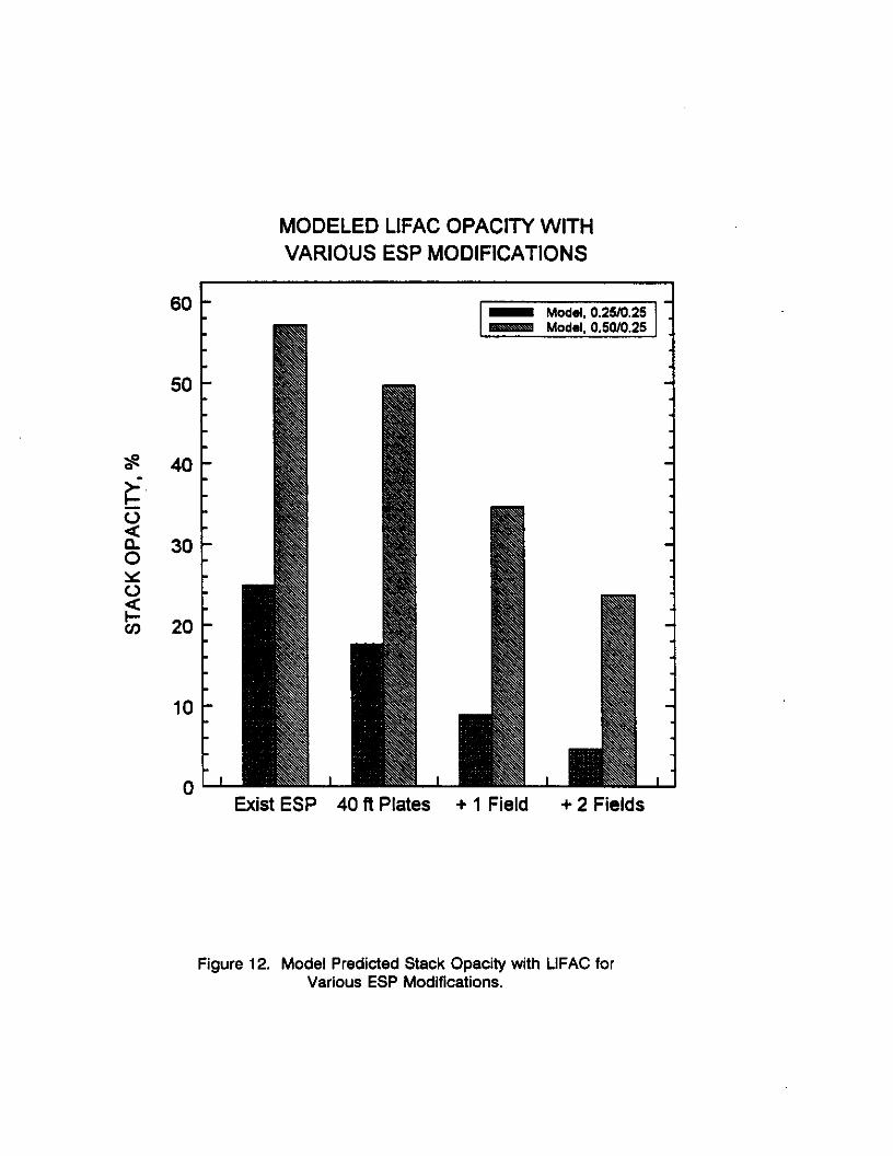
When non-ideal conditions of 0.25, 0.25 and 0.56, 0.25 are used to model LIFAC

operation with the existing Whitewater Valley Unit 2 ESP, the performance indicated in the

bottom half of Table 9a and by the leftmost group of bars on Figures 11 and 12 is

obtained. Particle emissions are predicted to be between 0.19 and 0.77 lb/l 0’ Stu, and

the opacity range is 25 to 57%. These levels are much worse than those measured

during the test program, but this is reasonable since they represent operation at 170’ F.

The opacity values assume that Unit 1 is off line and that only Unit 2 contributes to the

stack appearance. If Unit 1 were operating without serious problems, some dilution of

the mass concentration would occur to reduce the higher opacity levels. The reduction

in opacity with both units on line would be roughly equal to the ratio of the products of

each unit’s opacity and gas flow. This range of stack opacity is marginal with respect to

compliance. That is, based on the model projections, the existing ESP may or may not

operate in an acceptable range.

One factor which is working against the Unit 2 ESP with LIFAC is very high gas velocities

in the bottom of the ESP. Figure 13 shows the gas velocity profile measured at the inlet

of the ESP by EPSCON [7]. With an average gas velocity of 6.9 ft/sec, there were many

locations in the bottom half of the ESP which exceeded 10 ft/sec and a significant number

over 15 ft/sec’. Design gas velocities for modern ESPs are in the range of 3.5 fVsec and

values in excess of 5 ft/sec can degrade ESP performance by causing excessive particle

reentrainment. The high velocities can increase the magnitude of rapping puffs and

actually scour particles from the surface of collected dust layers. Although the ESP

model has a non-ideal parameter for gas flow distribution, this parameter does not

account for increased reentrainment from excessive velocity. Considering the gas

distribution in the Unit 2 ESP, the LIFAC model projections may be optimistic.

17

The effect on LIFAC performance of increasing the size of the Unit 2 ESP was also

estimated with the ESP model. Three modifications were considered, all of which include

increasing the collecting plate height from 30 to 40 feet. The plate height increase is

considered necessary to increase the ESP cross-sectional area and to reduce the gas

velocities. The first option was with that change only, while the other two included adding

either one or two 7.5 ft long collecting sections to the outlet of the ESP. The hardware

specifications of the modified ESP configurations are provided in Table 10, while the

model predictions are shown in Table 9b and in Figures 11 and 12. The model indicates

that two additional fields would be required to ensure that opacity remains below 30%

with LIFAC when Unit 1 is off line.

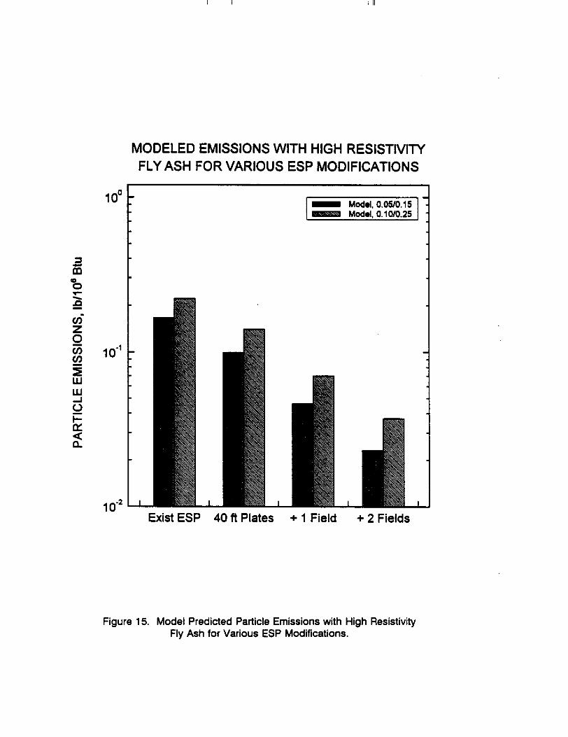
Projections of the performance of the modified ESP were also made with two different fly

ashes and are shown in Table 9b. Figures 13 and 14 show the model projections for the

baseline fly ash and Figures 15 and 15 provide the results with a very high resistivity dust.

The resistivity for the second case was assumed to be 1x10’* ohm-cm, and the ESP

electrical conditions were predicted from the EPRI database. The figures indicate that the

addition of two fields to the ESP should produce very good performance with most ashes

likely to be encountered.

18

I 1 I II

4. ANALYSIS AND RECOMMENDATIONS

The measurement program established that the source of, at the least, the majority of the

opacity excursion observed during LIFAC startup is related to emission of particles from

the ESP. Even when only water addition was used to drop the gas temperature with no

change in ESP inlet mass or particle size distribution, large increases in ESP emissions

occurred. Even if all of the SO, in the gas stream was condensed to sulfuric acid

droplets, which were collected in the sample train, that could account for only 1 O-20% of

the observed increase in mass.

The electrical operating conditions of the ESP were very good during the LIFAC tests

indicating that high dust resistivity was not limiting the performance of the ESP. There

was no indication that the excursions occurred because the fundamental collection

performance of the ESP was degraded. Therefore, the source of the excursion appears

to be a release of dust which has previously collected in the ESP. In fact, the vast

majority of the dust emitted during the initial excursion must be fly ash rather than LIFAC

dust. There are tens of thousands of pounds of dust residing on the ESP plates at any

time, and the release of only a small quantity of this dust would be required to create the

excursions observed.

The low temperature, high humidity conditions generated by LIFAC tend to reduce the

forces which hold the collected dust layer on the ESP electrodes through two avenues.

First, the dust resistivity is reduced which reduces the electrical clamping force. This

force is a function of the dust resistivity and the corona current through the dust layer.

At Whitewater Valley, the current density was increased only slightly (from 20 to 25

nA/cm2), while in-situ dust resistivity was reduced by an order of magnitude or more to

5x10’ ohm-cm (in-situ) or 5x10’ ohm-cm (Lab). This should result in a 2 to 3 order of

magnitude drop in the electrical holding force [8]. The second mechanism for reduction

in holding force is the reduction in tensile strength of the dust. The increase in relative

19

humidity from 12 to 23% decreased the tensile strength of the inlet samples by 25% and

the outlet samples by more than 50%.

Therefore, it appears that the most likely cause of the high opacity excursions is a

combination of reduced holding force and the high gas velocities in the ESP producing

reentrainment of previously collected dust. During baseline operation, stable dust layers

are created which balance the electrical and adhesive holding forces against the shearing

forces of the gas flow. When the conditions are suddenly changed to low temperature

and high humidity, the reduced electrical and tensile forces result in removal of dust from

the electrodes until a new stable (thinner) dust layer is reached. This problem could be

expected to reoccur if the conditions change again to increase relative humidity. The

small size, high gas velocities, and low current limit of the Whitewater Valley Unit 2 ESP

make this problem much more obvious than it might be in other situations.

The steady-state operation of the ESP during LIFAC will also be affected by the reduced

holding forces. Reduced holding force is a likely cause of the higher reentrainment

correction which must be used in the ESP model with most of the low-temperature

sorbent processes we have observed. The magnitude of the steady-state LIFAC

reentrainment problem has not yet been determined at Whitewater Valley. We

recommend that additional attempts to operate the ESP with LIFAC at 170’ F and no

bypass should be made during long-term tests with plenty of time allowed for transient

conditions to pass when changes are made. This could be accomplished by reducing

bypass until opacity increases, maintaining that setting until the transient passes, then

further reducing bypass until opacity increases again. This process should be iterated

until the bypass is closed or no further reductions in bypass can be made without

unacceptable opacity increases. At a minimum, several hours should be allowed for each

transient to pass before determining that no additional changes can be made.

Since both of the mechanisms which hold the dust on the collecting electrode are

inversely related ‘to relative humidity, decreasing the relative humidity should reduce

particle reentrainment and improve ESP operation with LIFAC. Figure 17 shows the

relationship between relative humidity and gas temperature for several moisture levels.

During the test program, acceptable ESP performance was measured at 196* F and

12.2% moisture, which corresponds to about 17% relative humidity. At the desired LIFAC

operating condition of 170’ F and 13.5% moisture, the relative humidity increases to 33%

because of the increased water and decreased temperature. Increasing the ESP

temperature to 205.F by using additional reheat would compensate for the higher

moisture content and provide approximately the same humidity as during the test

program. In our opinion, this is likely to result in improved performance.

From an economic standpoint, the cheapest source of heat in a coal-fired power plant

is hot flue gas. It is therefore logical to use this source of heat to obtain the additional

reheat necessary to reduce flue gas relative humidity and improve ESP performance. We

suggest bypassing a fraction of high-temperature flue gas around the air heater and

recombining it with the cool gas at the outlet of the LIFAC conditioning chamber. The

gas volume required would depend on the temperature of the hot gas. A major concern

in the design of such a system should be achieving good distribution of the hot gas to

avoid serious temperature gradients in the ESP which could degrade performance.

The poor gas flow distribution and high gas velocities in the ESP are certainly contributing

to reduced ESP performance under baseline conditions, but especially during LIFAC.

Durham has shown that increasing the ESP gas velocity from 3.6 to 4.1 ft/sec with a low-

temperature sorbent process increased particle penetration by a factor of 1.76 [lo]. With

the E-SO, process operating at 170-F on an ESP with SCA of 250 ft’/lOOO acfm,

Marchant measured a collection efficiency of 96% when flow distribution problems

produced gas velocities of 10 ft/sec in the bottom of the ESP [l 11. The Whitewater Valley

ESP gas velocities of lo-15 ft/.sec in the bottom of the ESP are believed to be largely

responsible for the poor performance. Unfortunately, we do not currently have a

technique for estimating the actual effect of high gas velocities on ESP emissions.

However, the evidence strongly indicates that improving the distribution will improve

21

performance, and we recommend that a flow study be performed and changes be made

to the flow distribution devices.

Although an increase in non-ideal conditions apparently occurs with all ESPs on low-

temperature sorbent processes, large, well designed ESPs with low gas velocities do not

appear to have serious particle emissibns problems at 17O.F [9]. The ESP model

indicates that increasing the plate height and adding two additional 7.5 ft. long fields to

the Whitewater Valley 2 ESP should result in acceptable performance with LIFAC. These

modifications would also provide excellent performance with essentially any fly ash

encountered in the future.

In summary, the following recommendations are made to evaluate and improve the

operation of the Whitewater Valley Unit 2 ESP during LIFAC:

1. Separate the excursion conditions from steady-state operation more clearly to

determine the extent of the steady-state reentrainment problem. Determine if

the ESP can operate at the design operating conditions if ESP temperature is

decreased gradually over a period of days with plenty of time for transient

conditions to pass.

2. Increase the amount of reheat to keep relative humidity in the range where

acceptable ESP performance is achieved.

3. Conduct a gas flow study and make modifications to improve the gas flow

distribution in the ESP as much as practical.

4. lf the preceding items do not result in acceptable performance, increasing the

ESP plate height to 40 ft and adding an additional 15 ft of collecting length to

the ESP should produce compliance performance.

22

5. REFERENCES

1.

2.

3.

4.

5.

6.

7.

8.

9.

10.

S. Matts and P. 0. Ohnfeldt, “Efficient Gas Cleaning with SF Electrostatic Precipitators”. AB Svenska Flaktfabriken Technical Bulletin, 1973.

J. L DuBard and R. S. Dahlin. Precipitator Performance Estimation Procedure. Electric Power Research Institute. Palo Alto, California. EPRI CS-5040. February 1987.

Cheney, J. L. and J. B. Homolya. “Sampling Parameters for Sulfate Measurements and Characterization,” Environ. Sci. & Technology, u(5) 584-588, 1979.

R. E. Bickelhaupt. A Technique for Predicting Fly Ash Resistivity. U. S. Environmental Protection Agency. Research Triangle Park, North Carolina. EPA-6OOJ7-79-204. July 1979.

R. E. Bickelhaupt. A Study to Improve a Technique for Predicting Fly Ash Resistivity with Emphasis on the Effect of Sulfur Trioxide. U. S. Environmental Protection Agency, Research Triangle Park, NC. EPA Report Number 600/7-86/010. NTIS PB86-178126. 1986.

M. G. Faulkner and J. L. DuBard. A Mathematical Model of Electrostatic Precipitation (Revision 3): Vol. I. U. S. Environmental Protection Agency. Research Triangle Park, North Carolina. EPA-600/7-84-069. July 1984.

“Measurement of Gas Velocity and Flow Distributions in the Richmond Department of Power and Light Whitewater Valley Station Unit 2 Electrostatic Precipitator on May 20, 1992. Report to Richmond Power and Light by EPSCON-FLS, Inc.

D. H. Pontius and T. R. Snyder, “Measurement of the Tensile Strength of Uncompacted Dust Aggregates”. Powder Technology, vol 68, ~159-162, 1991.

E. C. Landham. Jr., K. M. Cushing, Ralph F. Altman, Brian D. Larson, John B Doyle. “Effects of Spray Dryer Effluent on the Performance of the Laramie River Unit 3 ESP”. in Proceedings: Ninth Symposium on the Transfer and Utilization of Particulate Control Technology. Electric Power Research Institute, Palo Alto, CA. 1991.

M. D. Durham, et al. “Low-Resistivity Related ESP Performance Problems in Dry Scrubbing Applications”. Journal of Air and Waste Management Association, Vol. 40, No. 1, January 1990.

23

11. G. H. Marchant, et al. “Effects of E-SO, Technology on ESP Performance”. Final Report, EPA Cooperative Agreement No CR-81 4915-01-O. U.S. Environmental Protection Agency, Research Triangle Park, NC. May 1992.

Submitted by: E. C. Landham, Jr. Head, Control Systems Technology Section

Approved by: D. H. Pontius Director, Particulate S

24

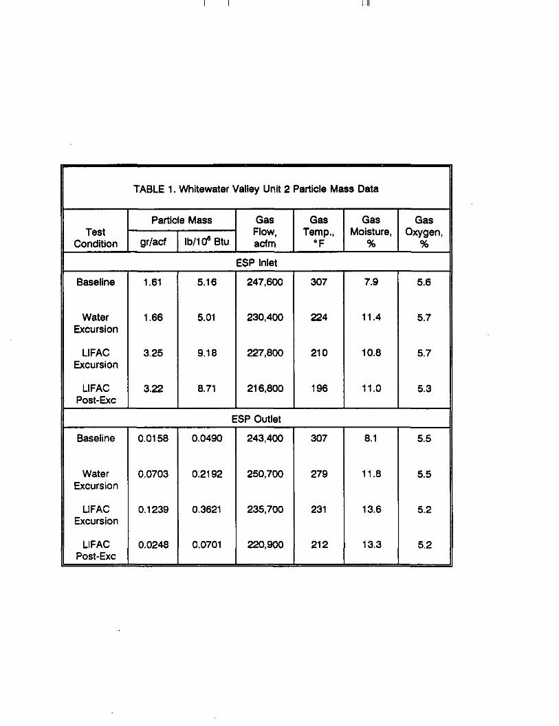
TABLE 1. Whitewater Valley Unit 2 Particle Mass Data

Test Condition

Baseline

Particle Mass GB Gas Gas Gas

lb/l 0’ 8tu Flow,

gr/acf Temp., Moisture, Oxygen,

acfm OF % %

ESP Inlet

1.61 5.16 247,600 307 7.9 5.6

Water Excursion

1.66 5.01 230,400 224 11.4 6.7

LIFAC Excursion

3.25 9.16 227,606 210 10.6 5.7

LIFAC Post-Exe

Baseline

3.22

0.0156

6.71 216,600 196 11.0 5.3

ESP Outlet

0.0490 243,400 307 6.1 5.5

Water Excursion

0.0703 0.2192 250,700 279 11.6 5.5

LIFAC Excursion

0.1239 0.3621 235,700 231 13.6 5.2

LIFAC Post-Exe

0.0248 0.0701 220,900 212 13.3 5.2

TABLE 2. Whitewater Valley Unit 2 ESP Performance Results

ESP Efficiency,

%

99.050

95.825

96.056

99.195

ESP Penetration,

%

0.950

4.375

3.944

0.805

Particle Emissions, lb/l O6 Etu

0.2192

0.3621

ESP” %I

cmlsec

82

26

27

ESP SCA,

ft?kacfm

58

II a. Effective Migration Velocity from Matts-Ohlnfeldt Equation with k=0.5 b. Measured in Stack with Both Units On-Line.

162

195

198

208

Stackb Opacity,

%

22

24

TABLE 3. Whitewater Valley Unit 2 SO, Results

Test Condition

Baseline

Gas Temperature,

‘F

306 308 311 307 307 299 302

Water 249 Excursion 234

LIFAC 238 223 211 210

1509 0.37 5.6 1539 0.31 5.3 1636 <0.3 5.1 1637 co.3 5.2

5.6 5.6 5.5 5.0 5.6 7.7 5.6

5.6 5.6

a. Actual duct concentration - not normalized for oxygen content.

TABLE 4. Chemical Composition of ESP Hopper Samples (Weight %)

Fly Ash LIFAC Dust

Inlet Outlet Inlet Outlet Hopper Hopper Hopper Hopper

U,O 0.03 0.04 0.02 0.02

N%O 0.62 0.79 0.55. 0.45

W 2.3 2.5 1.7 2.2

&lo 0.91 0.95 0.90 0.99

CaO 2.6 2.4 32.3 21.6

F%03 21.7 20.7 13.3 13.5

40, 22.2 23.4 14.8 19.8

SiO, 48.9 47.6 32.3 37.3

TiO, 1.1 1.2 0.74 0.91

PA 0.42 0.54 0.22 0.34

so3 0.58 0.51 4.6 4.6

LOI 3.8 5.4 5.0 4.4

Soluble SO;* 1 .o 1.4 5.6 5.0

B.E.T., m’lg 1.2 1.9 4.1 3.4

Equil. pH 8.8 6.2 11.1 10.9

Test Location

Main Duct

CSSP

TABLE 5. In-Situ Resistivity Data

Spark Resistivity, ohm-cm

2.76x1 0”

3.08x1 0”

2.32~10”

2.97x1 O’O

1.84x1 0”

3.07x1 o@

7.54x1 o9

1.49x1 O’O

1.66x1 O’O

4.55x1 O’O

1.75x1 0”

1.20x1 0”

5.40x1 O’O

2.26x1 0”

2.13x1 O’O

5.99x1 O’O

4.91x1 O’O

5.54x1 O’O

8.27x1 0’

6.81 Xl oQ

5.15x1 O’O

1.59x1 O’O

3.77x1 O’O

4.23x1 OS

<5x1 o9

1 90~10’~

TABLE 6. Whitewater Valley 2 ESP Electrical Conditions TABLE 6. Whitewater Valley 2 ESP Electrical Conditions

Condition

Baseline

Water Excursion

LIFAC Excursion

LIFAC Steady-

State

Current ESP Voltage, Current, Density, Field kV mA nAJcm’

1 42.7 193 18.5 2 43.4 180 17.3 3 47.1 203 19.5 4 49.7 240 23.0

1 43.4 265 25.4 2 43.4 268 25.0 3 43.3 255 24.5 4 47.0 270 25.9

1 43.0 255 24.5 2 41.6 260 25.0 3 41.8 260 25.0 4 45.3 280 26.9

1 43.3 255 24.5 2 41.9 266 25.4 3 42.0 260 25.0 4 46.0 270 25.9

TABLE 7. Tensile Strength of Whitewater Valley Dust Samples

Sample Type

Fly Ash Inlet 7.5 5.5

Fly Ash Outlet 32 15

LIFAC Dust Inlet 9.3 6.8

II LIFAC Dust I Outlet I >32 I 21 II

TABLE 8. Whitewater Valley 2 ESP Specifications

II Fields in Direction of Gas Flow

Collection Area per Field, e 11,280

Collecting Plate Spacing, in 11

II Collectina Plate Heioht. ft

II Collectino Plate Lenoth. ft

Wire-to-Wire Spacing, in

Number of Wires in Flow Direction

9

40

II Number of Gas Passaaes

II Number of Baffled Sections

TABLE 9a. Whitewater Valley 2 ESP Model Results

ESP Model Collection Particle Stack SCA. Non-Ideal Efficiency, Emissions,

ft?kacfm Opacity,

Conditions % lb/l 0’ Btu %

Model Comparison with Field Data using Standard Non-Ideal Conditions

Baseline 181 0.05, 0.15 98.76 0.060 13.7 0.10, 0.25 96.11 0.092 17.8

Water 195 0.05, 0.15 99.33 0.032 8.6 Excursion 0.10, 0.25 98.87 0.053 12.1

LIFAC 207 0.05, 0.15 99.41 0.052 10.8 Excursion 0.10, 0.25 99.00 0.089 15.8

LIFAC 207 0.05, 0.15 99.55 0.039 8.4 Steady-State 0.10, 0.25 99.20 0.069 12.7

Base ESP

40 ft High Plates

40 ft Plates +l Field

40 ft Plates +2 Fields

LIFAC Mode

207

278

345

414

‘rejections for

0.25, 0.25 0.50, 0.25

0.25, 0.25 0.50, 0.25

0.25, 0.25 0.50, 0.25

0.25, 0.25 0.50, 0.25

arious ESP Cc figurations

97.82 0.188 91.06 0.772

24.9 57.1

98.53 0.127 17.6 95.59 0.602 49.6

99.38 0.053 8.9 96.29 0.320 34.6

99.72 0.024 4.6 97.88 0.183 23.7

TABLE 9b. Whitewater Valley 2 ESP Model Results

ESP SCA,

ftzlkacfm

Model Non-Ideal

Conditions

Collection Particle Efficiency, Emissions,

% lb/l 0’ Btu

Stack Opacity,

%

Baseline Flv Ash Model Proiections for Various ESP Modifications

40 ff High Plates

40 ft Plates +l Field

40 ft Plates +2 Fields

241

302

362

0.05, 0.15 0.10, 0.25

0.05, 0.15 0.10, 0.25

0.05, 0.15 0.10, 0.25

99.35 98.89

99.75 99.53

99.90 99.79

0.032 0.054

0.012 0.023

0.005 0.010

8.0 11.2

3.5 5.5

1.6 2.8

Hiah Aesistivitv Flv Ash Model Proiections for Various ESP Modifications

Base ESP 181

40 ft High Plates

40 ft Plates +l Field

40 ft Plates +2 Fields

241

302

362

0.05, 0.15 96.59 0.10, 0.25 95.47

0.166 0.220

0.099 0.140

30.3 34.8

0.05, 0.15 97.97 0.10, 0.25 97.12

21.1 25.6

0.05, 0.15 99.05 0.046 11.9 0.10, 0.25 98.56 0.070 15.4

0.05, 0.15 99.53 0.023 6.7 0.10. 0.25 99.25 0.037 9.3

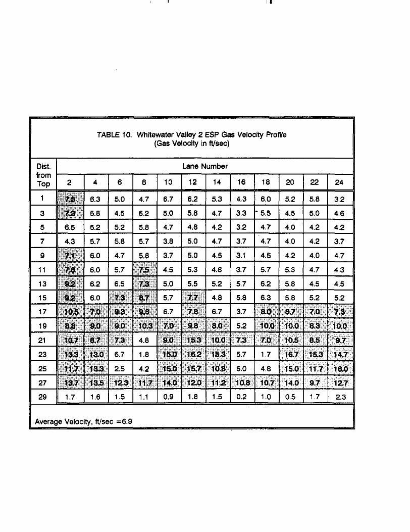
TABLE 10. Whitewater Valley 2 ESP Gas Velocity Profile (Gas Velocity in ft/sec)

Dist. Lane Number from Tnn 2 1 4 1 6 1 8 10 12 1 14 I 16 18 20 22 24

5.0 4.7 6.7 6.2 5.3 4.3 6.0 5.2 5.8 3.2 $$I 5,8 1 4.5 1 6.2 1 5.0 1 5.8 1 4.7 1 3.3 l-5.5 1 4.5 1 5.0 1 4.6 11

11 5 11 6.5 1 5.2 1 5.2 1 5.8 1 4.7 1 4.8 1 4.2 1 3.2 1 4.7 1 4.0 1 4.2 1 4.2 11

4.3 5.7 5.8 5.7 3.8 5.0 4.7 3.7 4.7 4.0 4.2 3.7

~~~~ 6,0 4.7 5.8 3,7 5.0 4.5 3.1 4.5 4.2 4.0 4.7 /

11 29 11 1.7 I 1.6 I 1.5 I 1.1 I 0.9 I 1.8 1 1.5 I 0.2 I 1.0 I 0.5 I 1.7 2.3 II

II Averaae Velacitv itlsec ~6.9 II

TABLE 11. ,Modified Whitewater Valley 2 ESP Specifications

40 ft High Plates

One Additional

Field

Two Additional

Fields

Fields in Direction of Gas Flow 4 5 6

Collection Area per Field, p 15,000 I 15,000 I 15,000

Collectina Plate Spacina. in 11 11 11

Collectino Plate Heiaht. ft I 40 I 40 I 40

Collecting Plate Length, ft 30 37.5 45

Wire-to-Wire Spacing, in 9 9 9

Number of Wires in Flow Direction 40 50 60

Number of Gas Passages 25 25 25

Number of Baffled Sections 4 5 6

WHITEWATER VALLEY UNIT 2 CUMULATIVE MASS SIZE DISTRIBUTION

3 1o’r E”

Ii t; 103r

3. 5 5 102r

ifi

10” - I I I 10” loo 10’ lo2

PARTICLE DIAMETER, micrometers

Figure 1. ESP Inlet Cumulative Mass Particle Size Distributions,

99.99

99.9

99

90

70

50

30

10

WHITEWATER VALLEY UNIT 2 CUMULATIVE PERCENT SIZE DISTRIBUTION

I I I I I

10-l loo 10’

PARTICLE DIAMETER, micrometers lo2

Figure 2. ESP Inlet Cumulative Percent Mass Particle Size Distributions.

WHlTEWATER VALLEY UNIT 2 DlFFERENTlAL MASS SlZE DISTRIBUTION

I fQEYff

10' ,p Ii I'

i n i T - I

10-l loo 10’

PARTICLE DIAMETER, micrometers lo2

Figure 3. ESP Inlet Differential Mass Particle Size Distributions.

MODEL 2 PREDICTED DUST RESISTIVITY WHITEWATER VALLEY FLY ASH

L 5 lo” : & z l0’O : 5 los: z 3

10"

0 OppmSO3 0 lppmSO3 A 4ppmSO3 n lOppmSO3 l 5.0~pmSO3

8.0% v&r Vapor

10" I I I. I. I c 1 ,"'.""'J

141 3 0 2.8 2.8 2.4 2.2 2.0 1.8 1.6 1.4 1000/K 183 233 291 359 441 541 666 826 Deg F

TEMPERATURE

Figure 4. Predicted Resistivity for Baseline Fly Ash.

MODEL 2 PREDICTED DUST RESISTNITY WHITEWATER VALLEY LIFAC DUST

10' F 10'

3 IO" IO" - I I I I I, I ,I I I , I , I, I I I I I I, I ,I I I , I , I, I

3.0 3.0 2.8 2.8 2.6 2.6 2.4 2.4 2.2 2.2 2.0 2.0 1.8 1.8 1.6 1.6 1.4 1.4 1000/K 1000/K 141 141 183 183 233 233 291 291 359 359 441 441 541 541 666 666 626 626 Deg F Deg F

TEMPERATURE

Figure 5. Predicted Ftesistivity for UFAC Dust.

10"

is "0 Z =

s 0 z 10-l

g

!!I u i=

I?

1o-2

MODELED LIFAC EMISSIONS WITH VARIOUS ESP MODIFICATIONS

Exist ESP 40 n Plates + 1 Field 1 -I

+ 2 Fields

Figure 11. Model Predicted Particle Emissions with LIFAC for Various ESP Modifications.

MODELED LIFAC OPACITY WITH VARIOUS ESP MODIFICATIONS

60 -

50 -

40 -

30 -

20 -

10 -

Od Exist ESP 40 n Plates

J + 1 Field + 2 Fields

Figure 12. Model Predicted Stack Opacity with LIFAC for Various ESP Modifications.

MODELED EMISSIONS WITH BASELINE FLYASH FOR VARlOm ESP MODIFICATIONS

I I

t

10-l -

1o-2 :

Exist ESP 40 n Plates L I

+ 1 Field

Figure 13. Model Predicted Particle Emissions with Baseline Fly Ash for Various ESP Modifications.

MODELED OPACITY WITH BASELINE FLYASH FOR VARIOUS ESP MODIFICATIONS

20 -

15 -

10 -

5-

O-l- Exist ESP 40 n Plates + 1 Field + 2 Fields

L

Figure 14. Model Predicted Stack Opacity with Basline Fly Ash for Various ESP Modifications.

loo

3 m "0 r

MODELED EMISSIONS WITH HIGH RESISTIVITY FLY ASH FOR VARIOUS ESP MODIFICATIONS

I

Exist ESP 40 ft Plates + 1 Field + 2 Fields

Figure 15. Model Predicted Particle Emissions with High Resistivity Fly Ash for Various ESP Modifications.

MODELED OPACITY WITH HIGH RESISTNITY FLY ASH FOR VARIOUS ESP MODIFICATIONS

30 -

20 -

10 -

n--L L Exist ESP 40 ft Plates + 1 Field + 2 Fields

Figure 16. Model Predicted Stack Opacity with High Resistivity Fly Ash for Various ESP Modifications.

EFFECT OF TEMPERATURE AND MOISTURE CONTENT ON RELATIVE HUMIDITY

,““,““,““1’“‘1”“1”“1”“1 60 -

_ 14%H20

tlO%KO\ \ 1

20 t- \ \\.\

IOI- -

I l..,.l,,,,l..,,‘I.,,‘.I..‘,,,,‘..,,’ 150 160 170 160 190 200 210 220

GAS TEMPERATURE, deg-F

Figure 17. The Effect of Temperature and Moisture Content on Relative Humidity.