Source Reconstruction

CRTI-02-0093RD Project Review MeetingCanadian Meteorological CentreAugust 22-23, 2006

Component 6: Inverse Source Determination and Bayesian Inference

urbanBLSurbanAEU

Bayesian inference for inverse source

determination

Adaptive sampling strategy

PSTP Component 6

• Localization of leakage of toxic gases and other pollutants (regulatory application)

• Terrorist incidents – localization of unknown source following event detection by network of CBR sensors (“electronic noses”) as quickly as possible

• Comprehensive Nuclear Test Ban Treaty (CTBT) – “sniffing” out clandestine nuclear tests (133Xe network of electronic noses)

Putative release event(s) Observations from sensors(electronic noses)

Source characteristics• emission rate• spatial location• on/off times• number of sources

Source reconstruction

Motivation for Source Reconstruction

Bayesian Inference: Foundations

)(),|()(

GDfIDPf NN

ForwardMap: G

Source-receptorrelationship

Modelerror

Inputerror

―

Stochasticuncertainty

Observationerror

CpCo

Noise:

BayesianInference

Prior

Likelihood

Posterior • input uncertainty (meteorology)• model errors• stochastic uncertainty• observation error

Noise:

Posterior distribution for source parameters: ),|()|(),|( IDPIPIDP

Estimate

Bayes’ rule

(Probabilisticdata fitting)

inference prior likelihood×

Application of Bayesian Inference for Inverse Source Determination

),,( ,)()()(),( ssssebs zyxxTtHTtHxxQtxS

)h (kg rate Emission

(h) time off Source

(h) time on Source

(m) Altitude

E) (deg Longitude

N) (deg Latitude

1- :

:

:

:

:

:

Q

T

T

z

y

x

e

b

s

s

s

),,,,,( QTTzyx ebsss

Assumed source distribution:

Source parameter vector

Infer source parameter vector using Bayes theorem:

likelihoodprior inference

),|()|()|(

),|()|(),|(

IDPIPIDP

IDPIPIDP

where

need to specify likelihood and prior to define posterior PDF for source parameters

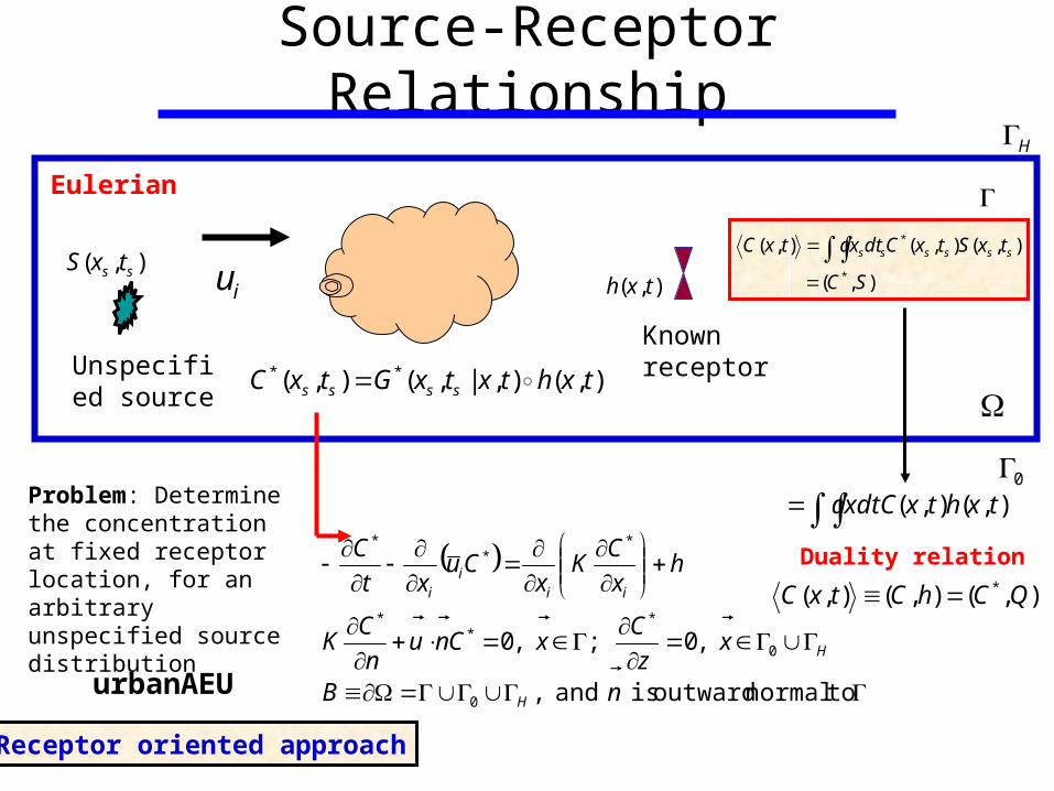
Source-Receptor Relationship

),( ss txS

Unspecified source

Knownreceptor

),( txh

iu

),(),|,(),( ** txhtxtxGtxC ssss

),(

),(),(),(

*

*

SC

txStxCdtxdtxC ssssss

,

,0 ; ,0

0

0

**

*

**

*

to normal outward is and nB

xz

CxCnu

n

CK

hx

CK

xCu

xt

C

H

H

iii

i

Problem: Determine the concentration at fixed receptor location, for an arbitrary unspecified source distribution

0

H

),(),( txhtxdtCxd

Duality relation

),(),(),( * QChCtxC

Eulerian

Receptor oriented approach

urbanAEU

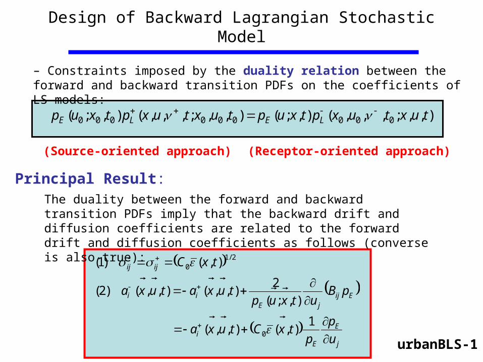
Design of Backward Lagrangian Stochastic Model

– Constraints imposed by the duality relation between the forward and backward transition PDFs on the coefficients of LS models:

Principal Result:The duality between the forward and backward transition PDFs imply that the backward drift and diffusion coefficients are related to the forward drift and diffusion coefficients as follows (converse is also true):

j

E

Ei

EijjE

ii

ijij

u

p

ptxCtuxa

pButxup

tuxatuxa

txC

1),(),,(

),;(

2),,(),,( )2(

),( )1(

0

2/10

),,;,,,(),;(),,;,,,(),;( 000000000 tuxtuxptxuptuxtuxptxup LELE

(Source-oriented approach) (Receptor-oriented approach)

urbanBLS-1

Examples of Source Reconstruction

• Joint Urban 2003 (JU2003)– Real cityscape (highly disturbed flow)

• European Tracer Experiment (ETEX)– Non-stationary, inhomogeneous flow over

complex terrain– Long-range dispersion on continental scales

Joint Urban 2003

Dual Concentration Field C*

*logC

Detector # 515(1-km sampling arc)

[C] = pptv[Q] = kg s-1

log C*

),( * SCC

urbanAEU

Example 1: (4 detectors)

N

Actual source location:

(xs , zs) = (3.2506,1.5537)

– estimated source location at one standard deviation:

093.0642.1

,0.6108.3

est

est

s

s

zss

xss

zz

xx

74

Detector

Source

Distributed drag force representation

0 1 2 3 4 50

0.1

0.2

0.3

0.4

0.5

0.6

0.7

0.8

0.9

1

Q (g s-1)

P(

Q |

D,I)

/ P0

0 1 2 3 4 5 60

0.1

0.2

0.3

0.4

0.5

0.6

0.7

0.8

0.9

1

xs

P(

x s | D

,I)/ P

0

Example 1: (4 detectors)

0 0.5 1 1.5 2 2.5 30

0.1

0.2

0.3

0.4

0.5

0.6

0.7

0.8

0.9

1

zs

P(

z s | D

,I)/ P

0

Actual xs :

3.2506

Actual zs :

1.5537

Actual Q :2.00 g s-1

– estimated source parameters at one standard deviation:

1

est

est

est

s g 41.054.1

,093.0642.1

,0.6108.3

Q

zss

xss

QQ

zz

xx

s

s

European Tracer Experiment

Inverse Source Determination for ETEX

• Concentration data extracted only from 10 sampling sites out of a total of 168 sampling sites

• Only 35 concentration time samples out of the total available 5,040 concentration samples were utilized for inversion (0.69% utilization of available data)

Degrees Longitude

De

gre

es

La

titu

de

Sampling sites:

F02: Alencon [2]

F19: Paris Orly [4]F21: Rennes [2]D10: Essen [4]

D13: Offenbach [5]

D19: Hof [3]

D34: Nurburg [7]

D44: Trier-Petrisberg [4]

D45: Wasserkuppe [3] CR04: Temelin [1]Map adapted from Platt et al. (2004)

Meteorological Data for ETEX

• Global Environmental Multiscale (GEM) model was executed in regional configuration with core resolution of 0.14° over Europe

• GEM produced a series of 3 and 6 h forecasts over the period of time corresponding to ETEX releases

• Initial data for GEM came from CMC Global data assimilation system

• Series of forecasts was used to “drive” backward LS particle model (MLPD-0) for calculation of C* (viz., GEM model outputs were used as “smart interpolator” of meteorological fields in space and time)

• C* fields were computed on a polar stereographic 229 229 grid over Europe (including UK) with a 15 km mesh length

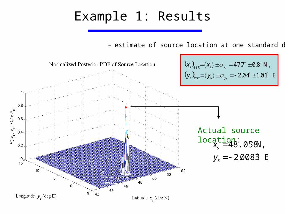
Example 1: Results

E01.104.2

,N 8.07.47

est

est

s

s

yss

xss

yy

xx

Actual source location:

E0083.2

N, 48.058

s

s

y

x

– estimate of source location at one standard deviation

Example 1: Results

h 2.59.13

,h 79.070.0

est

est

e

b

Tee

Tbb

TT

TT

Actual source on/off times:

h 0.13

h, 0.1

e

b

T

T

– estimate of source on/off times at one standard deviation

Example 1: Results

Actual source on/off times:

h 0.13

h, 0.1

e

b

T

T

Normalized Posterior PDFs of source on/off times

HPD interval (or, credible interval)(97.5% probability content)

h )0.20,25.0(

h, )5.2,0.0(

e

b

T

T

Source on

Source off (lower,upper)

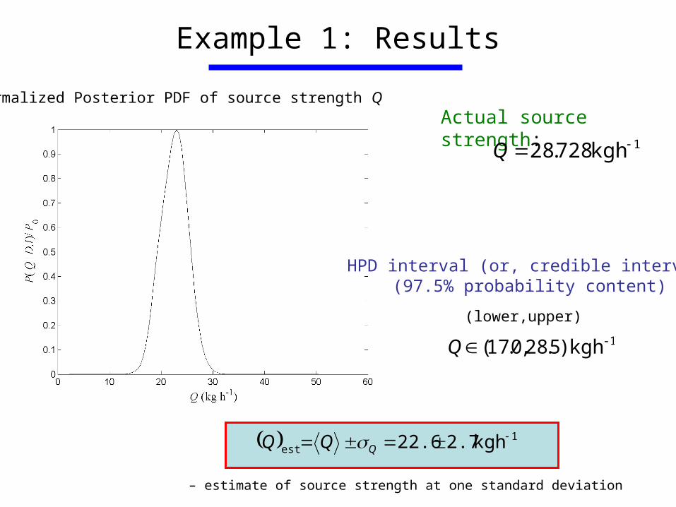
Example 1: Results

1est h kg 2.722.6 QQQ

Actual source strength:1h kg 728.28 Q

Normalized Posterior PDF of source strength Q

– estimate of source strength at one standard deviation

HPD interval (or, credible interval)(97.5% probability content)

-1h kg )5.28,0.17(Q

(lower,upper)

Conclusions

• Bayesian inference applied successfully to source reconstruction in complex environments involving highly disturbed wind fields (meteorological complexity)

• Methodology allows optimal estimates of source parameters along with their reliabilities, fully accounting for model and data uncertainty

• Future effort will extend methodology to more complex source configurations– Multiple sources– Area/volume sources– Moving sources

Generate a comprehensive tracer, meteorological and sensor dataset suitable for testing of current and future Sensor Data Fusion algorithms.

• Provide an abundance of tracer sensors and met instruments rather than an “optimal” placement. Sparser data sets can be had by ignoring unwanted measurements.

• Provide a variety of source types, strengths and locations. Include simultaneous emissions from different locations.

Objective:

FUsing Sensor Information from Observing Networks (FUSION) Field Trial 2007 (FFT 07)

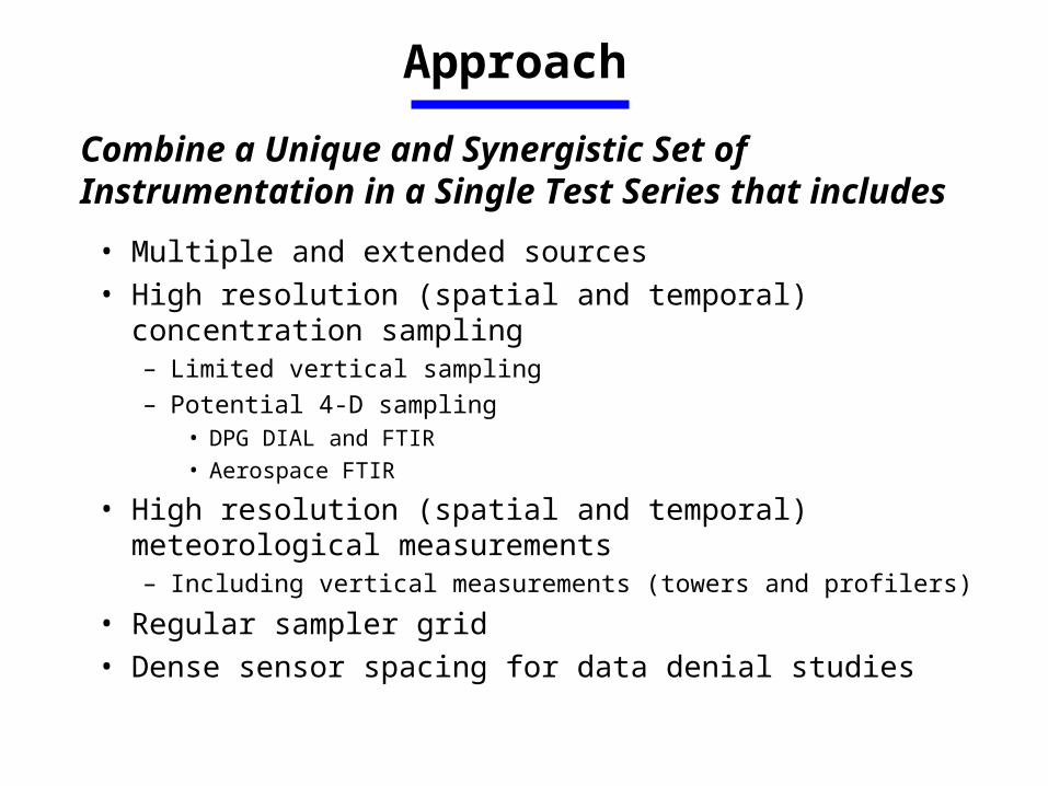
• Multiple and extended sources• High resolution (spatial and temporal) concentration sampling

– Limited vertical sampling– Potential 4-D sampling

• DPG DIAL and FTIR • Aerospace FTIR

• High resolution (spatial and temporal) meteorological measurements– Including vertical measurements (towers and profilers)

• Regular sampler grid• Dense sensor spacing for data denial studies

Combine a Unique and Synergistic Set of Instrumentation in a Single Test Series that includes

Approach

1 km

1 km

2 km

20 PWIDs to display real-time winds on the test bed

25 3D sonics for high temporal (10 Hz) resolution wind data close to high resolution samplers.

100 dPID propylene samplers in 1 km square grid for high temporal resolution (1 Hz) of propylene concentration data.

Propylene release areas

32 meter towers with sonics and other sensors at five levels (2, 4, 8, 16 and 32m).

Other Possible Instrumentation (locations TBD): DPG SAMS sites, DPG 924-MHz radar wind profiler and mini-sodars, DPG FM/CW boundary layer radar, Net SW/LW radiometers, DPG tethersonde, Aerospace FTIR, MIRAN detectors.

23 UK UVICS on the down-wind perimeter with high sensitivity (10 ppb) and temporal resolution (1-10 Hz) in the region of lowest expected concentration.

Details of the Proposed FUSION Test-bed