Source coding and channel requirements for unstable processes

Anant Sahai, Sanjoy Mittersahai@eecs.berkeley.edu, mitter@mit.edu

Abstract

Our understanding of information in systems has been based on the foundation of memoryless processes.Extensions to stable Markov and auto-regressive processesare classical. Berger proved a source coding theoremfor the marginally unstable Wiener process, but the infinite-horizon exponentially unstable case has been open sinceGray’s 1970 paper. There were also no theorems showing what is needed to communicate such processes acrossnoisy channels.

In this work, we give a fixed-rate source-coding theorem for the infinite-horizon problem of coding an expo-nentially unstable Markov process. The encoding naturallyresults in two distinct bitstreams that have qualitativelydifferent QoS requirements for communicating over a noisy medium. The first stream captures the information thatis accumulating within the nonstationary process and requires sufficient anytime reliability from the channel used tocommunicate the process. The second stream captures the historical information that dissipates within the processand is essentially classical. This historical informationcan also be identified with a natural stable counterpart tothe unstable process. A converse demonstrating the fundamentally layered nature of unstable sources is given bymeans of information-embedding ideas.

Index Terms

Nonstationary processes, rate-distortion, anytime reliability, information embedding

Department of Electrical Engineering and Computer Science at the University of California at Berkeley. A few of these results werepresented at ISIT 2004 and a primitive form of others appeared at ISIT 2000 and in his doctoral dissertation.

Department of Electrical Engineering and Computer Science at the Massachusetts Institute of Technology. Support for S.K. Mitter wasprovided by the Army Research Office under the MURI Grant: Data Fusion in Large Arrays of Microsensors DAAD19-00-1-0466 and theDepartment of Defense MURI Grant: Complex Adaptive Networks for Cooperative Control Subaward #03-132 and the National ScienceFoundation Grant CCR-0325774.

1

Source coding and channel requirements for unstable processes

I. I NTRODUCTION

The source and channel models studied in information theoryare not just interesting in their own right,but also provide insights into the architecture of reliablecommunication systems. Since Shannon’s work,memoryless sources and channels have always been at the baseof our understanding. They have providedthe key insight of separating source and channel coding withthe bit rate alone appearing at the interface[1], [2]. The basic story has been extended to many differentsources and channels with memory forpoint-to-point communication [3].

However, there are still many issues for which information theoretic understanding eludes us. Net-working in particular has a whole host of such issues, leading Ephremides and Hajek to entitle theirsurvey article “Information Theory and Communication Networks: An Unconsummated Union!” [4]. Theycomment:

The interaction of source coding with network-induced delay cuts across the classical network layers and hasto be better understood. The interplay between the distortion of the source output and the delay distortion inducedon the queue that this source output feeds into may hold the secret of a deeper connection between informationtheory. Again, feedback and delay considerations are important.

Real communication networks and networked applications are quite complicated. To move toward aquantitative and qualitative of understanding of the issues, tractable models that exhibit at least some ofthe right qualitative behavior are essential. In [5], [6], the problem of stabilization of unstable plants acrossa noisy feedback link is considered. There, delay and feedback considerations become intertwined and thenotion of feedback anytime capacity is introduced. To stabilize an otherwise unstable plant over a noisychannel, not only is it necessary to have a channel capable ofsupporting a certain minimal rate, but thechannel when used with noiseless feedback must also supporta high enough error-exponent (called theanytime reliability) with fixed delay in a delay-universal fashion. This turns out to be a sufficient conditionas well, thereby establishing a separation theorem for stabilization. In [7], upper bounds are given forthe fixed-delay reliability functions of DMCs with and without feedback, and these bounds are shown tobe tight for certain classes of channels. Moreover, the fixed-delay reliability functions with feedback areshown to be fundamentally better than the traditional fixed-block-length reliability functions.

While the stabilization problem does provide certain important insights into interactive applications,the separation theorem for stabilization given in [5], [6] is coarse — it only addresses performance as abinary valued entity: stabilized or not stabilized. All that matters is the tail-behavior of the closed-loopprocess. To get a more refined view in terms of steady-state performance, this paper instead considersthe corresponding open-loop estimation problem. This is the seemingly classical question of lossy sourcecoding for anunstablescalar Markov processes — mapping the source into bits and then seeing what isrequired to communicate such bits using a point-to-point communication system.

A. Communication of Markov processes

Coding theorems for stable Markov and auto-regressive processes under mean-squared-error distortionare now well established in the literature [8], [9]. We consider real-valued Markov processes, modeled as

Xt+1 = λXt +Wt (1)

whereWtt≥0 are white andX0 is an independent initial condition uniformly distributedon [−Ω0

2,+Ω0

2]

whereΩ0 > 0 is small. The essence of the problem is depicted in Fig. 1: to minimize the rate of theencoding while maintaining an adequate fidelity of reconstruction. Once the source has been compressed,the resulting bitstreams can presumably be reliably communicated across a wide variety of noisy channels.

The infinite-horizon source-coding problem is to design a source code minimizing the rateR usedto encode the process while keeping the reconstruction close to the original source in an average sense

2

'

&

$

% '

&

$

%

- -

?

?

---

-

Reliable

Xt

Source

Wt

SourceCodingLayer

Xt

Estimates

SourceDecoder(s)

“Bitstreams”Interface

ChannelDecoder

LayerTransmission

ChannelNoisy

ChannelEncoderEncoder(s)

Source

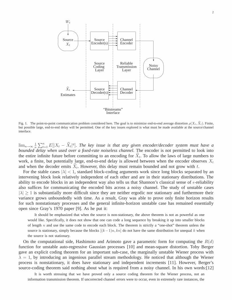
Fig. 1. The point-to-point communication problem considered here. Thegoal is to minimize end-to-end average distortionρ(Xt, bXt). Finite,but possible large, end-to-end delay will be permitted. One of the key issues explored is what must be made available at the source/channelinterface.

limn→∞1n

∑n

t=1E[|Xt − Xt|η]. The key issue is that any given encoder/decoder system must have a

bounded delay when used over a fixed-rate noiseless channel.The encoder is not permitted to look intothe entire infinite future before committing to an encoding for Xt. To allow the laws of large numbers towork, a finite, but potentially large, end-to-end delay is allowed between when the encoder observesXt

and when the decoder emitsXt. However, this delay must remain bounded and not grow witht.For the stable cases|λ| < 1, standard block-coding arguments work since long blocks separated by an

intervening block look relatively independent of each other and are in their stationary distributions. Theability to encode blocks in an independent way also tells us that Shannon’s classical sense ofǫ-reliabilityalso suffices for communicating the encoded bits across a noisy channel. The study of unstable cases|λ| ≥ 1 is substantially more difficult since they are neither ergodic nor stationary and furthermore theirvariance grows unboundedly with time. As a result, Gray was able to prove only finite horizon resultsfor such nonstationary processes and the general infinite-horizon unstable case has remained essentiallyopen since Gray’s 1970 paper [9]. As he put it:

It should be emphasized that when the source is non-stationary, the above theorem is not as powerful as onewould like. Specifically, it does not show that one can code a long sequence by breaking it up into smaller blocksof lengthn and use the same code to encode each block. The theorem is strictly a “one-shot” theorem unless thesource is stationary, simply because the blocks[(k−1)n, kn] do not have the same distribution for unequalk whenthe source is not stationary.

On the computational side, Hashimoto and Arimoto gave a parametric form for computing theR(d)function for unstable auto-regressive Gaussian processes[10] and mean-square distortion. Toby Bergergave an explicit coding theorem for an important sub-case, the marginally unstable Wiener process withλ = 1, by introducing an ingenious parallel stream methodology.He noticed that although the Wienerprocess is nonstationary, it does have stationary and independent increments [11]. However, Berger’ssource-coding theorem said nothing about what is required from a noisy channel. In his own words:[12]

It is worth stressing that we have proved only a source codingtheorem for the Wiener process, not aninformation transmission theorem. If uncorrected channelerrors were to occur, even in extremely rare instances, the

3

user would eventually lose track of the Wiener process completely. It appears (although it has never been proved)that, even if anoisy feedback link were provided, it still would not be possible to achieve a finite [mean squarederror] per letter ast→∞.

In an earlier conference work [13] and the first author’s dissertation [14], we gave a variable rate codingtheorem that showed theR(d) bound is achievable in the infinite-horizon case if variable-rate codes areallowed. The question of whether or not fixed-rate and finite-delay codes could be made to work was leftopen, and is resolved here along with a full information transmission theorem.

B. Asymptotic equivalences and direct reductions

Beyond the technical issue of fixed or variable rate lies a deeper question regarding the nature of“information” in such processes. [15] contains an analysisof the traditional Kalman-Bucy filter in whichcertain entropic expressions are identified with the accumulation and dissipation of information within afilter. No explicit source or channel coding is involved, butthe idea of different kinds of information flowsis raised through the interpretation of certain mutual information quantities. In the stabilization problemof [5], it is hard to see if any qualitatively distinct kinds of information are present since to an externalobserver, the closed-loop process is stable.

Similarly, the variable-rate code given earlier in [13], [14] does not distinguish between kinds ofinformation since the same high QoS requirements were imposed on all bits. However, it was clear thatall the bitsdo not requirethe same treatment since there are examples in which access to an additionallower reliability medium can be used to improve end-to-end performance [16], [14]. The true nature ofthe information within the unstable process was left open and while exponentially unstable processescertainly appeared to be accumulating information, there was no way to make this interpretation preciseand quantify the amount of accumulation.

In order to understand the nature of information, this paperbuilds upon the “asymptotic communicationproblem equivalence” perspective introduced at the end of [5]. This approach associates communicationproblems (e.g. communicating bits reliably at rateR or communicating iid Gaussian random variables toaverage distortion≤ d) with the set of channels that are good enough to solve that problem (e.g. noisychannels with capacityC > R). This parallels the “asymptotic computational problem equivalence”perspective in computational complexity theory [17] except that the critical resource shifts from compu-tational operations to noisy channel uses. The heart of the approach is the use of “reductions” that showthat a system made to solve one communication problem can be used as a black box to solve anothercommunication problem. Two problems are asymptotically equivalent if they can be reduced to each other.

The equivalence perspective is closely related to the traditional source/channel separation theorems. Themain difference is that traditional separation theorems give a privileged position to one communicationproblem — reliable bit-transport in the Shannon sense — and use reductions in only one direction: fromthe source to bits. The “converse” direction is usually proved using properties of mutual information. In[18], [19], we give a direct proof of the “converse” for classical problems by showing the existence ofrandomized codes that embed iid message bits into iid seeming source symbols at rateR. The embeddingis done so that the bits can be recovered with high probability from distorted reconstructions as long asthe average distortion on long blocks stays below the distortion-rate functionD(R). Similar results areobtained for the conditional distortion-rate function. This equivalence approach to separation theoremsconsiders the privileged position of reliable bit-transport to be purely a pedagogical matter.

This paper uses the results from [18], [19] to extend the results of [5] from the control context to theestimation context. We demonstrate that the problem of communicating an unstable Markov process towithin average distortiond is asymptotically equivalent to a pair of communication problems: classicalreliable bit-transport at a rate≈ R(d) − log2 |λ| and anytime-reliable bit-transport at a rate≈ log2 |λ|.This gives a precise interpretation to the nature of information flows in such processes.

4

C. Outline

Section II states the main results of this paper. A brief numerical example for the Gaussian case isgiven to illustrate the behavior of such unstable processes. The proofs follow in the subsequent sections.

Section III considers lossy source coding for unstable Markov processes with the driving disturbanceWt

constrained to have bounded support. A fixed-rate code at a rate arbitrarily close toR(d) is constructedby encoding process into two simultaneous fixed-rate message streams. The first stream has a bit-ratearbitrarily close tolog2 |λ| and encodes what is needed from the past to understand the future. It capturesthe information that is accumulating within the unstable process. The other stream encodes those aspectsof the past that are not relevant to the future and so capturesthe purely historical aspects of the unstableprocess in a way that meets the average distortion constraint. This second stream can be made to have arate arbitrarily close toR(d)− log2 |λ|.

Section IV then examines this historical information more carefully by looking at the process formallygoing backward in time. TheR(d) curve for the unstable process is shown to have a shape that isthestable historical part translated bylog2 |λ| to account for the unstable accumulation of information.

Section V first reviews the fact that random codes exist achieving anytime reliability over noisy channelseven without any feedback. Then, forη-difference distortion measures, an anytime reliability> η log2 |λ|is shown to be sufficient to encode the first bitstream of the code of Section III across a noisy channel. Thesecond bitstream is shown to only require classical Shannonǫ-reliability. This completes the reduction ofthe lossy-estimation problem to a two-tiered reliable bit-transportation problem and resolves the conjectureposed by Berger regarding an information transmission theorem for unstable processes.

Section VI tackles the other direction. The problem of anytime-reliable bit-transport is directly reducedto the problem of lossy-estimation for a decimated version of the unstable process. This is done usingthe ideas in [5], reinterpreted as information-embedding and shows that the higher QoS requirements forthe first stream are unavoidable for these processes. A second stream of messages is then embedded intothe historical segments of the unstable process and this stream is recovered in the classical Shannonǫ-reliable sense.Exponentially unstable Markov processes are thus the first nontrivial examples of stochasticprocesses that naturally generate two qualitatively distinct kinds of information.

In Section VII, the results are then extended to cover the Gauss-Markov case with the usual squared-error distortion. Although the proofs are given in terms of Gaussian processes and squared error, theresults actually generalize to anyη-distortion as well as driving noise distributionsW that have at leastan exponentially decaying tail.

This paper focuses throughout on scalar Markov processes for clarity. It is possible to extend all thearguments to cover the general autoregressive moving average (ARMA) case. The techniques used tocover the ARMA case are discussed in the control context in [6] where a state-space formulation is used.A brief discussion of how to apply those techniques is present here in Section VIII.

II. M AIN RESULTS

A. Performance bound in the limit of large delays

To defineR(d) for unstable Markov processes, the infinite-horizon problem is viewed as the limit of asequence of finite-horizon problems:

Definition 2.1: Given the scalar Markov source given by (1), thefinite n-horizon version of the sourceis defined to be the random variablesXn−1

0 = (X0, X1, . . . , Xn−1).Definition 2.2: Theη−distortionmeasure isρ(Xi, Xi) = |Xi−X|

η. It is an additive distortion measurewhen applied to blocks.

The standard information-theoretic rate-distortion function for the finite-horizon problem usingη-difference distortion is:

RXn (d) = inf

P(Y n−10 |Xn−1

0 ): 1n

Pn−1i=0 E[|Xi−Yi|η ]≤d

1

nI(Xn−1

0 ;Y n−10 ) (2)

5

We can consider the blockXn1 as a single vector-valued random variable~X. TheRX

n (d) defined by

(2) is related toR ~X1 (d) by RX

n (d) = 1nR~X1 (nd) with the distortion measure on~X given by ρ( ~X, ~X) =∑n−1

i=0 |Xi − X|η.

The infinite-horizon case is then defined as a limit:

RX∞(d) = lim inf

n→∞RXn (d) (3)

The distortion-rate functionDX∞(R) is also defined in the same manner, except that the mutual-

information is fixed and the distortion is what is infimized.

B. The stable counterpart to the unstable process

It is insightful to consider what the stable counterpart to this unstable process would be. There is anatural choice, just formally turn the recurrence relationship around and flip the order of time. This givesthe “backwards in time process” governed by the recursion

←−X t = λ−1←−X t+1 − λ

−1Wt. (4)

This is purely a formal reversal. In place of an initial condition X0, it is natural to consider a←−X n for

some timen and then consider time going backwards from there. Since|λ−1| < 1, this is a stable Markovprocess and falls under the classical theorems of [9].

C. Encoders and decoders

For notational convenience, time is synchronized between the source and the channel. Thus both delayand rate can be measured against either source symbols or channel uses.

Definition 2.3: A discrete time channelis a probabilistic system with an input. At every time stept, ittakes an inputat ∈ A and produces an outputct ∈ C with probabilityp(Ct|at1, c

t−11 ) where the notationat1

is shorthand for the sequence(a1, a2, . . . , at). In general, the current channel output is allowed to dependon all inputs so far as well as on past outputs.

The channel ismemorylessif conditioned onat, the random variableCt is independent of any otherrandom variable in the system that occurs at timet or earlier. So all that needs to be specified ispt(Ct|at).The channel is memoryless and stationary ifpt(Ct|at) = p(Ct|at) for all times t.

Definition 2.4: A rate R source-encoderEs is a sequence of mapsEs,i. The range of each map isa single bitbi ∈ 0, 1 if it is a pure source encoder and is from the channel input alphabetA if it is a

joint source-channel encoder. Thei-th map takes as input the available source symbolsX⌊ i

R⌋

1 .Similarly, a rate R channel-encoderEc without feedbackis a sequence of mapsEc,t. The range of

each map is the channel input alphabetA. The t-th map takes as input the available message bitsB⌊Rt⌋1 .

Randomized encodersalso have access to random variables denoting the common randomness availablein the system. This common randomness is independent of the source and channel.

Definition 2.5: A delayφ rateR source-decoderis a sequence of mapsDs,t. The range of each mapis just an estimateXt for the t-th source symbol. For pure source decoders, thet-th map takes as input theavailable message bitsB⌊(t+φ)R⌋

1 . For joint source-channel decoders, it takes as input the available channeloutputsCt+φ

1 . Either way, it can seeφ time units beyond the time when the desired source symbol firsthad a chance to impact its inputs.

Similarly, a delayφ rate R channel-decoderis a sequence of mapsDc,i. The range of each map isjust an estimateBi for the i-th bit taken from0, 1. The i-th map takes as input the available channel

outputsC⌈ i

R⌉+φ

1 which means that it can seeφ time units beyond the time when the desired message bitfirst had a chance to impact the channel inputs.

Randomized decodersalso have access to the random variables denoting common randomness.

6

-AA AA AA AA AA AA AA AA AA AA AA AA AA AA AA AA AA AA AA AA AA AA AA AA AA AA

-

? ? ? ? ? ? ? ? ?

? ? ?? ? ? ? ? ? ? ? ? ?

A1 A2 A3 A4 A5 A6 A7 A8 A9 A10A11A12A13A14A15A16A17A18A19A20A21A22A23A24A25A26

C1 C2 C3 C4 C5 C6 C7 C8 C9 C10 C11 C12 C13 C14 C15 C16 C17 C18 C19 C20 C21 C22 C23 C24 C25 C26

fixed delayd = 7

bB6bB8

bB1bB2

bB3bB4

bB5bB7

bB9

B1 B2 B3 B4 B5 B6 B7 B8 B9 B10 B11 B12 B13

Fig. 2. The timeline in a rate12

delay7 channel code. Both the encoder and decoder must be causal soAi and bBi are functions only ofquantities to the left of them on the timeline. If noiseless feedback is available,the Ai can also have an explicit functional dependence onthe Ci−1

1 that lie to the left on the timeline.

SourceDecoder

- -- -Xt Source

Encoder bXt

Coded BitstreamsR1

R2

Fig. 3. The source-coding problem of translating the source into two simultaneous bitstreams of fixed ratesR1 andR2. End-to-end delayis permitted but must remain bounded for all time. The goal is to getR1 ≈ log2 |λ| andR2 ≈ R(d) − log2 |λ|.

The timeline is illustrated in Fig. 2 for channel coding and asimilar timeline holds for either puresource coding or joint source-channel coding.

For a specific channel, the maximum rate achievable for a given sense of reliable communication iscalled the associated capacity. Shannon’s classicalǫ-reliability requires that for a suitably large end-to-enddelayφ, the probability of error on each bit is below a specifiedǫ.

Definition 2.6: A rateR anytime communication systemover a noisy channel is a single channel encoderEc and decoderDφc family for all end-to-end delaysφ.

A rateR communication system achievesanytime reliabilityα if there exists a constantK such that:

P(Bi1(t) 6= Bi

1) ≤ K2−α(t− iR

) (5)

holds for everyi. The probability is taken over the channel noise, the message bitsB, and all of thecommon randomness available in the system. If (5) holds for every possible realization of the messagebits B, then we say that the system achievesuniform anytime reliabilityα.

Communication systems that achieveanytime reliability are calledanytime codesand similarly foruniform anytime codes.

The important thing to understand about anytime reliability is that it is not considered to be a proxy usedto study encoder/decoder complexity as traditional reliability functions often are [8]. Instead, the anytimereliability parameterα indexes a sense of reliable transmission for a bitstream in which the probabilityof bit error tends to zero exponentially as time goes on.

D. Main results

The first result concerns the source coding problem illustrated in Fig. 3 for unstable Markov processeswith bounded-support driving noise.

Theorem 2.1:Assume both the source encoder and source decoder can be randomized. Given theunstable (|λ| > 1) scalar Markov process from (1) driven by independent noiseWtt≥0 with bounded

7

support, it is possible to encode the process to average fidelity E[|Xi − Xi|η] arbitrarily close tod using

two fixed-rate bitstreams and a suitably high end-to-end delay φ.The first stream (called thecheckpoint stream) can be made to have rateR1 arbitrarily close tolog2 |λ|

while the second (called thehistorical stream) can have rateR2 arbitrarily close toRX∞(d)− log2 |λ|.

Proof: See Section III.

In a very real sense, the first stream in Theorem 2.1 represents an initial description of the process tosome fidelity, while the second represents a refinement of thedescription [20]. These two descriptionsturn out to be qualitatively different when it comes to communicating them across a noisy channel.

Theorem 2.2:Suppose that a communication system provides uniform anytime reliabilityα > η log2 |λ|for the checkpoint message stream at bit-rateR1. Then given sufficient end-to-end delayφ, it is possibleto reconstruct the checkpoints to arbitrarily high fidelityin the η-distortion sense.Proof: See Section V-B.

Theorem 2.3:Suppose that a communication system can reliably communicate message bits meetingany bit-error probabilityǫ given a long enough delay. Then, that communication system can be used toreliably communicate the historical information message stream generated by the fixed-rate source codeof Theorem 2.1 in that the expected end-to-end distortion can be made arbitrarily close to the distortionachieved by the code over a noiseless channel.Proof: See Section V-C.

The Gauss-Markov case with mean squared error is covered by corollaries:Corollary 2.1: Assume both the encoder and decoder are randomized and the finite end-to-end delayφ

can be chosen to be arbitrarily large. Given an unstable (|λ| > 1) scalar Markov process (1) driven by iidGaussian noiseWtt≥0 with zero mean and varianceσ2, it is possible to encode the process to averagefidelity E[|Xi − Xi|

2] arbitrarily close tod using two fixed-rate bitstreams.The checkpoint stream can be made to have rateR1 arbitrarily close tolog2 |λ| while the historical

stream can have rateR2 arbitrarily close toRX∞(d)− log2 |λ|.

Proof: See Section VII-A.

Corollary 2.2: Suppose that a communication system provides us with the ability to carry two messagestreams. One at rateR1 > log2 |λ| with uniform anytime reliabilityα > 2 log2 |λ|, and another withclassical Shannon reliability at rateR2 > RX

∞(d) − log2 |λ| whereRX∞(d) is the rate-distortion function

for an unstable Gauss-Markov process with unstable gain|λ| ≥ 1 and squared-error distortion.Then it is possible to successfully transport the two-stream code of Corollary 2.1 using this communi-

cation system by picking a sufficiently large end-to-end delay φ. The mean squared error of the resultingsystem will be as close tod as desired.Proof: See Section VII-B.

Theorems 2.2 and 2.3 together with the source code of Theorem2.1 combine to establish a reductionof thed-lossy joint source/channel coding problem to the problem of communicating message bits at rateR(d) over the same channel, wherein a substream of message bits atrate≈ log2 |λ| is given an anytimereliability of at leastη log2 |λ|. This reduction is in the sense of Section VII of [5]: any channel that isgood enough to solve the second pair of problems is good enough to solve the first problem.

The asymptotic relationship between the forward and backward rate-distortion functions is captured inthe following theorem.

Theorem 2.4:Let X be the unstable Markov process of (1) with|λ| > 1 and let the stable backwards-in-time version from (4) be denoted

←−X . Assume that the iid driving noiseW has a Riemann-integrable

density fW and there exists a constantK so thatE[|∑t

i=1 λ−iWi|

η] ≤ K for all t ≥ 1. Furthermorefor the purpose of calculating the rate-distortion functions below, assume that for the backwards-in-timeversion is initialized with

←−X n = 0. Let Q∆ be the uniform quantizer that maps its input to the nearest

neighbor of the formk∆ for integerk.

8

R←−X∞(d) =(a) lim

∆→0limn→∞

R←−X |Q∆(

←−X0)

n (d) =(b) limn→∞

R←−X |←−X0n (d) =(c) R

X∞(d)− log2 |λ|. (6)

or expressed in terms of distortion-rate functions forR > log2 |λ|:

DX∞(R) = D

←−X∞(R− log2 |λ|).

This implies that the process generally undergoes a phase transition from infinite to bounded averagedistortion at the critical ratelog2 |λ|.Proof: See Section IV-B.

Notice that there are no explicitly infinite distortions in the original setup of the problem. Consequently,the appearance of infinite distortions is interesting as is the abrupt transition from infinite to finitedistortions around the critical rate oflog2 |λ|. This abrupt transition gives a further indication that thereis something fundamentally nonclassical about the ratelog2 |λ| information inside the process.

To make this precise, a converse is needed. Classical rate-distortion results only point out that themutual information across the communication system must beat leastR(d) on average. However, as [21]points out, having enough mutual information is not enough to guarantee a reliable-transport capacitysince the situation here is not stationary and ergodic. The following theorem gives the converse, but addsan intuitively required additional condition that the probability of excess average distortion over any longenough segment can be made as small as desired.

Theorem 2.5:Consider the unstable process given by (1) with the iid driving noiseW having aRiemann-integrable densityfW satisfying the conditions of Theorem 2.4.

Suppose there exists a family (indexed by window sizen) of joint source-channel codes(Es,Ds)) sothat then-th member of the family has reconstructions that satisfy

E[|Xkn − Xkn|η] ≤ d (7)

for every positive integerk. Furthermore, assume the family collectively also satisfies

limn→∞

supτ≥0P(

1

n

τ+n−1∑

i=τ

|Xi −Xi|η > d) = 0 (8)

so that the probability of excess distortion can be made arbitrarily small on long enough blocks.Then for anyR1 < log2 |λ|, α < η log2 |λ|, R2 < RX

∞(d) − log2 |λ|, Pe > 0, the channel must supportthe simultaneous carrying of a bit-rateR1 priority message stream with anytime reliabilityα along witha second message stream of bit-rateR2 with a probability of bit error≤ Pe for some end-to-end delayφ.Proof: See Section VI-A.

Note that a Gaussian disturbanceW is covered by Theorems 2.4 and 2.5, even if the difference distortionmeasure is not mean squared-error.

E. An example and comparison to the sequential rate distortion problem

In the case of Gauss-Markov processes with squared-error distortion, Hashimoto and Arimoto in [10]give an explicit way of calculatingR(d). Tatikonda in [22], [23] gives a similar explicit lower boundto the rate required when the reconstructionXt is forced to be causal in that it can only depend onXj

observations forj ≤ t.Assuming unit variance for the driving noiseW andλ > 1, Hashimoto’s formula is parametric in terms

of the water-filling parameterκ and for the Gauss-Markov case considered here simplifies to:

D(κ) =1

2π

∫ π

−πmin

[κ,

1

1− 2λ cos(ω) + λ2

]dω,

R(κ) = log2 λ+1

2π

∫ π

−πmax

[0,

1

2log2

1

κ(1− 2λ cos(ω) + λ2)

]dω. (9)

9

0

0.2

0.4

0.6

0.8

1

0.5 1 1.5 2 2.5 3 3.5Rate (in bits)

Squ

ared

err

or d

isto

rtio

n

"Sequential" Rate−distortion (obeys causality)

Rate−distortion curve (non−causal)

Stable counterpart (non−causal)

Fig. 4. The distortion-rate curves for an unstable Gauss-Markov process withλ = 2 and its stable backwards-version. The stable andunstableD(R) curves are related by a simple translation by1 bit per symbol.

The rate-distortion function for the stable counterpart given in (4) has a water-filling solution that isidentical to 9, except without thelog2 λ term in theR(κ)! Thus, in the Gaussian case with squared errordistortion direct calculation verifies the claim

RX∞(d) = log2 λ+R

←−X∞(d)

from Theorem 2.4.For the unstable process, Tatikonda’s formula for causal reconstructions is given by

Rseq(d) =1

2log2(λ

2 +1

d). (10)

Fig. 4 shows the distortion-rate frontier for both the original unstable process and backwards stableprocess. It is easy to see that the forward and backward process curves are translations of each other.In addition, the sequential rate-distortion curve for the forward process is qualitatively distinct.Dseq(R)goes to infinity asR ↓ log2 λ while D(R) approaches a finite limit.

The results in this paper show that the lower curve for the regular distortion-rate frontier can beapproached arbitrarily closely by increasing the acceptable (finite) end-to-end delay. This suggests that ittakes some time for the randomness entering the unstable process throughW to sort itself into the twocategories of fundamental accumulation and transient history. The difference in the resulting distortion isnot that significant at high rates, but becomes unboundedly large as the rate approacheslog2 λ. It is openwhether similar information-embedding theorems similar to Theorem 2.5 exist that give an operationalmeaning to the gap betweenRseq(d) andR(d). If a communication system can be used to satisfy distortiond in a causal way, does that mean the underlying communicationresources also must be able to supportmessages at this higher rateRseq(d)?

III. T WO STREAM SOURCE ENCODING: APPROACHINGR(d)

This section proves Theorem 2.1.

10

Recursively decode

dithered checkpoints exactly

-

6

?

-

6

?

-

6

?

Source Encoder

Source Decoder

bX

X

high priority stream

Conditionally encode

(checkpoints)

by subtracting checkpoints

Random

“dither”

Recursively encode checkpoints

with fixed rate dithered code

Add checkpoints back Conditionally decode the

normalized superblock

Normalize (make iid)

historical blocks normalized superblock

to desired fidelity

to get reconstruction

for original signal

low priority stream

(history in between)

Fig. 5. A flowchart showing how to do fixed-rate source coding for Markov sources using two streams and how the streams are decoded.

A. Proof strategy

The code for proving Theorem 2.1 is illustrated in Fig. 5. Without loss of generality, assumeλ = |λ| > 1to avoid the notational complication of keeping track of thesign.• Look at time in blocks of sizen and encode the values of endpoints(Xkn−1, Xkn) recursively to

very high precision using raten(log2 λ + ǫ1) per pair. Each blockXkn, Xkn+1, . . . , X(k+1)n−1 willhave encoded checkpoints(Xkn, Xkn+n−1) at both ends.

• Use the encoded checkpointsXkn at the start of the blocks to transform the process segments inbetween (the history) so that they look like an iid sequence of finite horizon problems~X.

• Use the checkpointsXkn+n−1 at the end of the blocks as side-information to encode the historyto fidelity d at a rate ofn(RX

∞(d)− log2 λ+ ǫ2 + o(1)) per block.• “Stationarize” the encoding by choosing a random starting offset so that no timest area priori more

vulnerable to distortion.The source decoding proceeds in the same manner and first recovers the checkpoints, and then uses them

as known side-information to decode the history. The two arethen recombined to give a reconstructionof the original source to the desired fidelity.

The above strategy follows the spirit of Berger’s encoding[11]. In Berger’s code for the Wiener process,the first stream’s rate is negligible relative to that of the second stream. In our case, the first stream’s rateis significant and cannot be averaged away by using large blocks n.

The detailed constructions and proof for this theorem are inthe next few subsections, with sometechnical aspects relegated to the appendices.

B. Recursively encoding checkpoints

This section relies on the assumption of bounded support forthe driving noise|Wt| ≤Ω2, but does

not care about any other property of theWtt≥0 like independence or stationarity. The details of thedistortion measure are also not important for this section.

11

Proposition 3.1:Given the unstable (λ > 1) scalar Markov process of (1) driven by noiseWtt≥0

with bounded support, and any∆ > 0, it is possible to causally and recursively encode checkpointsspaced byn so that|Xkn − Xkn| ≤

∆2

. For anyR1 > log2 λ, this can be done with ratenR1 bits percheckpoint by choosingn large enough. Furthermore, if an iid sequence of independent pairs of continuousuniform random variablesΘi,Θ

′ii≥0 is available to both the encoder and decoder for dithering, the errors

(Xkn−1−Xkn−1, Xkn−Xkn) can be made an iid sequence of pairs of independent uniform random variableson [−∆

2,+∆

2].

Proof: First, consider the initial condition atX0. It can be quantized to be within an interval of size∆by usinglog2⌈

Ω0

∆⌉ bits.

With a block length ofn, the successive endpoints are related by:

X(k+1)n = λnXkn + [λn−1

n−1∑

i=0

λ−iWkn+i] (11)

The second term[· · · ] on the left of (11) can be denotedWk and bounded using

|Wk| = |λn−1

n−1∑

i=0

λ−iWkn+i| ≤ |λn−1|

n−1∑

i=0

λ−iΩ

2< λn

Ω

2(λ− 1). (12)

Proceed by induction. Assume thatXkn satisfies|Xkn−Xkn| ≤∆2

. This clearly holds fork = 0. Withoutany further information, it is known thatX(k+1)n must lie within an interval of sizeλn∆ + λn Ω

λ−1. By

usingnR′1 bits (whereR′1 is chosen to guarantee an integernR′1) to encode where the true value lies, theuncertainty is cut by a factor of2nR

′

1 . To have the resulting interval of size∆ or smaller, we must have:

∆ ≥ 2−nR′

1λn(∆ +Ω

(λ− 1)).

Dividing through by∆2−nR′

1λn and taking logarithms gives

n(R′1 − log2 λ) ≥ log2(1 +Ω

∆(λ− 1)).

EncodingXkn−1 given Xkn requires very little additional rate since|Xkn−1−λ−1Xkn| < Ω+∆ and so

log2⌈Ω∆

+1⌉ < log2(2+ Ω∆

) additional bits are good enough to encode both checkpoints.Putting everythingtogether in terms of the originalR1 gives

R1 ≥ max

(log2 λ+

log2(1 + Ω∆(λ−1)

) + log2(2 + Ω∆

)

n,log2⌈

Ω0

∆⌉

n

). (13)

It is clear from (13) that no matter how small a∆ we choose, by picking ann large enough the rateR1 can get as close tolog2 λ as desired. In particular, pickingn = K(log2

1∆

)2 works with largeK andsmall ∆.

To get the uniform nature of the final errorXkn − Xkn, subtractive dithering can be used [24]. Thisis accomplished by adding a small iid random variableΘk, uniform on [−∆

2,+∆

2], to theXkn, and only

then quantizing(Xkn + Θk) to resolution∆. At the decoder,Θk is subtracted from the result to getXkn.Similarly for Xkn−1. This results in the checkpoint error sequence(Xkn−1 − Xkn−1, Xkn − Xkn) beingiid uniform pairs over[−∆

2,+∆

2]. These pairs are also independent of all theWt and initial conditionX0.

In what follows, we always assume that∆ is chosen to be of high fidelity relative to the target distortiond (e.g. For squared-error distortion, this means that∆2 ≪ d.) as well as small relative to the the initialcondition so∆≪ Ω0.

12

C. Transforming and encoding the history

Having dealt with the endpoints, focus attention on the historical information between them. Here thebounded support assumption is not needed for theWt, but the iid assumption is important. First, theencoded checkpoints are used to transform the historical information so that each historical segment looksiid. Then, it is shown that these segments can be encoded to the appropriate fidelity and rate when thedecoder has access to the encoded checkpoints as side information.

1) Forward transformation:The simplest transformation is to effectively restart the process at everycheckpoint and view time going forward. This can be considered normalizing each of the historicalsegmentsX(k+1)n−1

kn to (X(k,i), 0 ≤ i ≤ n− 1) for k = 0, 1, 2, . . ..

X(k,i) = Xkn+i − λiXkn (14)

For eachk, the blockXk = X(k,i)0≤i≤n−1 satisfiesX(k,i+1) = λX(k,i) + W(k,i). By dithered quan-tization, the initial condition (i = 0) of each block is a uniform random variable of support∆ that isindependent of all the other random variables in the system.The initial conditions are iid across thedifferent k. Thus, except for the initial condition, the blocksXk are identically distributed to the finitehorizon versions of the problem.

Since∆ < Ω0, eachXk block starts with a tighter initial condition than the original X process did.Since the initial condition is uniform, this can be viewed asa genie-aided version of the original problemwhere a genie reveals a few bits of information about the initial condition. Since the initial conditionenters the process dynamics in a linear way and the distortion measureρ depends only on the difference,this implies that the new process with the smaller initial condition requires no more bits per symbol toachieve a distortiond than did the original process. Thus:

RXn (d)−

1 + log2Ω0

∆

n≤ R

eXn (d) ≤ RX

n (d)

for all n andd. So in the limit of largen

ReX∞(d) = RX

∞(d). (15)

In simple terms, the normalized history behaves like the finite horizon version of the problem whennis large.

2) Conditional encoding:The idea is to encode the normalized history between two checkpointsconditioned on the ending checkpoint. The decoder has access to the exact values of these checkpointsthrough the first bitstream.

For a givenk, shift the encoded ending checkpointX(k+1)n−1 to

Zqk = X(k+1)n−1 − λ

n−1Xkn. (16)

Zqk is clearly available at both the encoder and the decoder since it only depends on the encoded

checkpoints. Furthermore, it is clear that

X(k,n−1) − Zqk = (X(k+1)n−1 − λ

n−1Xkn)− (X(k+1)n−1 − λn−1Xkn) = X(k+1)n−1 − X(k+1)n−1

which is a uniform random variable on[−∆2,+∆

2]. ThusZq

k is just a dithered quantization to∆ precisionof the endpointX(k,n−1).

Define the conditional rate-distortion functionRX|Zq,Θ∞ (d) for the limit of long historical blocksXn−1

k,0

conditioned on their quantized endpoint as

RX|Zq ,Θ∞ (d) = lim inf

n→∞

1

ninf

P(Y n−10 | eXn−1

0 ,Zq ,Θ): 1n

Pn−1i=0 E[| eXi−Yi|η]≤d

1

nI(Xn−1

0 ;Y n−10 |Zq,Θ). (17)

13

Proposition 3.2:Given an unstable (λ > 1) scalar Markov processXk,t obeying (1) and whosedriving noise satisfiesE[|

∑t

i=1 λ−iWi|

η] ≤ K for all t ≥ 1 for some constantK, together with itsencoded endpointZq

k obtained byΘ-dithered quantization to within a uniform random variablewith smallsupport∆, the limiting conditional rate-distortion function

RX|Zq,Θ∞ (d) = RX

∞(d)− log2 λ. (18)

Proof: See Appendix C.

The case of driving noise with bounded support clearly satisfies the conditions of this proposition sincegeometric sums converge. The conditional rate-distortionfunction in Proposition 3.2 has a correspondingcoding theorem:

Proposition 3.3:Given an unstable (λ > 1) scalar Markov processXt given by (1) together withits n-spaced pairs of encoded checkpointsX obtained by dithered quantization to within iid uniformrandom variables with small support∆, for every ǫ4 > 0 there exists anM large enough so that aconditional source-code exists that maps a lengthM superblock of the historical informationXk0≤k<Minto a superblockTk0≤k<M satisfying

1

M

M−1∑

k=0

1

n

n∑

j=1

E[ρ(X(k,j), T(k,j))] ≤ d+ ǫ4. (19)

By choosingn large enough, the rate of the superblock code can be made as close as desired toRX∞(d)− log2 λ if the decoder is also assumed to have access to the encoded checkpointsXkn.

Proof: M of the Xk blocks are encoded together using conditioning on the encoded checkpoints at theend of each block. The pair(Xk, Z

qk) have a joint distribution, but are iid acrossk by the independence

properties of the subtractive dither and the driving noiseW(k,i). Furthermore, theX(k,i) are bounded andas a result, the all zero reconstruction results in a boundeddistortion on theX vector that depends onn.Even without the bounded support assumption, Theorem 2.4 reveals that there is a reconstruction basedon theZq

k alone that has bounded average distortion where the bound does not even depend onn.Since the side informationZq

k is available at both encoder and decoder, the classical conditional rate-distortion coding theorems of [25] tell us that there existsa block-lengthM(n) so that codes exist satisfying(19). The rate can be made arbitrarily close toRX|Zq ,Θ

n (d). By letting n get large, Proposition 3.2 revealsthat this rate can be made as close as desired toRX

∞(d)− log2 λ.

D. Putting history together with checkpoints

The next step is to show how the decoder can combine the two streams to get the desired rate/distortionperformance.

The rate side is immediately obvious since there islog2 λ from Proposition 3.1 andRX∞(d) − log2 λ

from Proposition 3.3. The sum is as close toRX∞(d) as desired. On the distortion side, the decoder runs

(14) in reverse to get reconstructions. Suppose thatT(k,i) are the encoded transformed source symbolsfrom the code in Proposition 3.3. ThenXkn+i = T(k,i) + λiXkn and soXkn+i − Xkn+i = X(k,i) − T(k,i).Since the differences are the same, so is the distortion.

E. “Stationarizing” the code

The underlyingXt process is non-stationary so there is no hope to make the encoding truly stationary.However, as it stands, only the average distortion across each of theMn length superblocks is close todin expectation giving the resulting code a potentially “cyclostationary” character. Nothing guarantees thatsource symbols at every time will have the same level of expected fidelity. To fix this, a standard trickcan be applied by making the encoding have two phases:

14

• An initialization phase that lasts for a randomT time-steps.T is a random integer chosen uniformlyfrom 0, 1, . . .Mn−1 based on common randomness available to the encoder and decoder. During thefirst phase, all source symbols are encoded to fidelity∆ recursively using the code of Proposition 3.1with n = 1.

• A main phase that applies the two-part code described above but starts at timeT + 1.The extra rate required in the first phase is negligible on average since it is a one-time cost. This takes

a finite amount of time to drain out through the rateR1 message stream. This time can be considered anadditional delay that must be suffered for everything in thesecond phase. Thus it adds to the delay ofnrequired by the causal recursive code for the checkpoints. The rest of the end-to-end delay is determinedby the total lengthMn of the superblock chosen inside Proposition 3.3.

Let di be such that the original super-block code gives expected distortiondi at positioni ranging from0 to Mn − 1. It is known from Proposition 3.3 that1

Mn

∑Mn−1i=0 di ≤ d + ǫ4. Because the first phase is

guaranteed to be high fidelity and all other time positions are randomly and uniformly assigned positionswithin the superblock of sizeMn, the expected distortionE[|Xi− Xi|

η] ≤ d+ ǫ4 for every bit positioni.The code actually does better than that since the probability of excess average distortion over a long

block is also guaranteed to go to zero. This property is inherited from the repeated use of independentconditional rate-distortion codes in the second stream [25].

This completes the proof of Theorem 2.1.

IV. T IME-REVERSAL AND THE ESSENTIAL PHASE TRANSITION

It is interesting to note that the distortion of the code in the previous section turns out to be entirelybased on the conditional rate-distortion performance for the historical segments. The checkpoints merelycontribute alog2 λ term in the rate.

The nature of historical information in the unstable Markovprocess described by (1) can be exploredmore fully by transforming the historical blocks going locally backward in time. The informationaldistinction between the process going forward and the purely historical information parallels the conceptsof information production and dissipation explored in the context of the Kalman Filter [15].

First, the original problem is formally decomposed into forward and backward parts. Then, Theorem 2.4is proved.

A. Endpoints and history

It is useful to think of the original problem as being broken down into two analog sub-problems:1) Then-endpoint problem:This is the communication of the processXkn where each sample arrives

everyn time steps and the samples are related to each other through (11) with Wk being iid and havingthe same distribution asλn−1

∑n−1i=0 λ

−iWi.This process must be communicated so thatE[|Xkn − Xkn|

η] ≤ K for some performanceK. This isessentially a decimated version of the original problem.

2) The conditional history problem:The stable←−X process defined in (4) can be viewed in blocks

of lengthn. The conditional history problem is thus the problem of communicating an iid sequence ofn-vectors ~X−k = (

←−X k,1, . . . ,

←−X k,n−1) conditioned on iidZk that are known perfectly at the encoder and

decoder. The joint distribution of~X−, Z are given by:

Z = −n−1∑

i=0

λ−iWi

←−X n−1 = −λ−1Wn−1←−X t = λ−1←−X t+1 − λ

−1Wt

15

where the underlyingWt are iid. Unrolling the recursion gives←−X t = −

∑n−1−ti=0 λ−i−1Wt+i. TheZ is

thus effectively the endpointZ =←−X 0. The vectors~X−k are made available to the encoder everyn time

units along with their corresponding side-informationZk. The goal is to communicate these to a receiverthat has access to the side-informationZk so that 1

n

∑n−1i=1 E[ρ(

←−X k,i, X

−k,i)] ≤ d for all k.

The relevant rate distortion function for the above problemis the conditional rate-distortion function

R←−X |Zn (d). The proof of Theorem 2.1 in the previous section involves a slightly modified version of the

above where the side-informationZ is known only to some quantization precision∆. The quantized

side-information isZq = Q(∆,Θ)(Z). The relevant conditional rate-distortion function isR←−X |Zq ,Θn (d).

3) Reductions back to the original problem:It is obvious how to put these two problems together toconstruct an unstableXt stream: the endpoints problem provides the skeleton and theconditional historyinterpolates in between. To reduce the endpoints problem tothe original unstable source communicationproblem, just use randomness at the transmitter to sample from the interpolating distribution and fill inthe history.

To reduce the conditional history problem to the original unstable source communication problem, justuse the iidZk to simulate the endpoints problem and use the interpolating~X history to fill out Xt.Because the distortion measure is a difference distortion measure, the perfectly known endpoint processallows us to translate everything so that the same average distortion is attained.

B. Rate-distortion relationships proved

Theorem 2.4 tells us that the unstable|λ| > 1 Markov processes are nonclassical only as they evolveinto the future. The historical information is a stable Markov process that fleshes out the unstable skeletonof the nonstationary process. This fact also allows a simplification in the code depicted in Fig. 5. Since theside-information does not impact the rate-distortion curve for the stable historical process, the encodingof the historical information can be done unconditionally and on a block-by-block basis. There is no needfor superblocks.

The remainder of this section proves Theorem 2.4.Proof:

1) (a): It is easy to see thatR←−X∞(d) = limn→∞R

←−X |Q∆(

←−X0)

n (d) since the endpoint←−X 0 is distributed

like −∑t

i=1 λ−iWi and has a finiteη-th moment by assumption. By Lemma B.1 (in the Appendix), the

entropy ofQ∆(←−X 0) is bounded below a constant that depends only on the precision ∆. This finite number

is then amortized away asn→∞.2) (b): Next, we show

lim∆→0

R←−X |Q∆(

←−X0)

∞ (d) = limn→∞

R←−X |←−X0n (d). (20)

For notational convenience, letZq = Q∆(←−X 0). First, R

←−X |←−X0n (d) is immediately bounded above by

R←−X |Zq

n (d) since knowledge of←−X 0 exactly is better than knowledge of only the quantizedZq. To get a

lower bound, imagine a hypothetical problem that is one time-step longer and consider the choice betweenknowing

←−X 0 to fine precision∆ or knowing

←−X−1 exactly.

R←−X

n−1

0 |←−X−1(d) ≥(i) R←−X

n−1

0 |←−X−1,Zq

(d)

≥(ii) R←−X

n−1

0 |←−X−1,Zq ,Cγ ,Gδ ,W

′′

δ (d)

where (i) and (ii) above hold since added conditioning can only reduce the conditional rate-distortionfunction, andCγ, Gδ,W

′′δ are from the following lemma applied to the hypothesizedW−1 driving noise.

Lemma 4.1:Given a random variableW with densityfW , arbitrary1 > γ > 0, there exists aδ > 0 sothat it is possible to realizeW as

W = (1− Cγ)(Gδ + Uδ) + CγW′′δ (21)

16

where• Cγ is a Bernoulli random variable with probabilityγ of being 1.• Uδ is a continuous uniform random variable on[− δ

2,+ δ

2].

• Gδ andW ′′δ are some random variables whose distributions depend onfW , δ, γ.

• Cγ, Uδ, Gδ,W′′δ are all independent of each other.

Proof: See Appendix A.

Pick γ small and then choose∆≪ δ. Notice that←−X−1 = λ−1←−X 0−λ

−1(1−Cγ)(Gδ +Uδ)+λ−1CγW′′δ

whereCγ, Uδ, Gδ,W′′δ are independent of each other as well as the entire vector

←−X

n−1

0 . Because the←−X t

process is Markov, the impact of the observations←−X−1, Z

q, Cγ, Gδ,W′′δ on the conditional rate-distortion

function is factored entirely through the posterior distribution for←−X 0.

There are two cases:• Cγ = 1 The value for

←−X 0 is entirely revealed by the observations. The posterior is aDirac delta.

• Cγ = 0 There are two independent measurements of←−X 0. The first is the quantizationZq. The second

is λ←−X−1 +Gδ =

←−X 0 − Uδ. This is just

←−X 0 blurred by uniform noise.

It is useful to view them as coming one after the other. After seeingZq = Q∆(←−X 0) = z1, the posterior

distributionP(←−X 0|Z

q = z1) has support only within[z1 −∆2, z1 + ∆

2].

The distributionP(Z2|Zq = z1) for the second observationZ2 =

←−X 0 − Uδ conditioned on the first

observation has a pair of interesting properties. First, ithas support only on[z1 −δ+∆

2, z1 + δ+∆

2].

Second, the distribution is uniform over the interval(z1 −δ−∆

2, z1 + δ−∆

2) since theP(

←−X 0|Z

q = z1)has support with total span∆≪ δ.Consider the posteriorP(

←−X 0|Z

q = z1, Z2 = z2) for z2 ∈ (z1−δ−∆

2, z1 + δ−∆

2) and apply Bayes rule:

P(←−X 0 ≤ x|Zq = z1, Z2 = z2) =

P(←−X 0 ≤ x, Z2 = z2|Z

q = z1)

P(Z2 = z2|Zq = z1)

= δP(←−X 0 ≤ x, Z2 = z2|Z

q = z1)

=(δP(Z2 = z2|Z

q = z1,←−X 0 ≤ x)

)P(←−X 0 ≤ x|Zq = z1)

= P(←−X 0 ≤ x|Zq = z1).

So if it lands in this region, the second observation is useless. Notice thatUδ ∈ ( δ−2∆2, δ−2∆

2) forces

the second observation to be inside this region. Thus the second observation is useless with probability

at least(1− γ) δ−2∆δ

regardless of what the actual←−X

n−1

0 are.Define a new hypothetical observationZ ′ that with probability(1− γ) δ−2∆

δis just equal toZq and is

equal to←−X 0 otherwise. The above tells us that this is a more powerful observation than than the original

(←−X−1, Z

q, Cγ , Gδ,W′′δ ). Thus

R←−X

n−1

0 |←−X−1(d) ≥ R←−X

n−1

0 |Z′

(d)

= (1− γ)δ − 2∆

δR←−X

n−1

0 |Zq

(d) +

(1− (1− γ)

δ − 2∆

δ

)R←−X

n−1

0 |←−X0(d)

≥ (1− γ)δ − 2∆

δR←−X

n−1

0 |Zq

(d).

17

Simple algebra then reveals that

R←−X |Zq

n =1

nR←−X

n−1

0 |Zq

(d)

≤δR←−X

n−1

0 |←−X−1(d)

n(1− γ)δ − 2∆

=δ(n+ 1)

n(1− γ)δ − 2∆R←−X |Zn+1 (d).

Taking the limits ofn→∞, ∆δ→ 0, δ → 0, γ → 0 establishes the desired result.

Notice that an identical argument works to show that

lim∆→0

limn→∞

RX|Zq

n (d) = limn→∞

RX|Xnn (d)

for the forward unstable process. It does not matter if it is conditioned on the exact endpoint or a finelyquantized version of it. Notice also that the argument is unchanged if the quantization was dithered ratherthan undithered.

3) (c): This follows almost immediately from (18) from Proposition3.2. The only remaining task isto show that

R←−X |Z∞ (d) = RX|Z

∞ (d).

It is clear that the iidZk in the “conditional history” problem are just scaled-down (by a factor ofλ−(n−1)) versions of theWk from the “endpoints” problem. The forward~Xk = (Xk,1, . . . , Xk,n−1) canbe recovered using a simple translation of~X−k by the vector(Zk, λZk, . . . , λn−1Zk) since

Xt =t−1∑

i=0

λt−i−1Wi

=n−1∑

i=0

λt−i−1Wi −n−1∑

i=t

λt−i−1Wi

= λt−1

n−1∑

i=0

λ−iWi −

n−1−t∑

i=0

λ−i−1Wt+i

= λt−1Z +←−X t.

Similarly, the conditional history problem can be recovered from the forward one by another simpletranslation of ~Xk by the vector(−λ−(n−1)Zk, . . . ,−λ

−1Zk,−Zk).Thus, the problem of encoding the conditional history to distortion d conditioned on its endpoints is

the same whether we are considering the unstable forward or stable backwards processes.4) Phase transition:At rates strictly less thanlog2 λ, the distortion for the originalX process is

necessarily infinite. This is shown in Lemma 6.2 where finite distortion implies the ability to carry≈ log2 λ bits through the communication medium.

V. QUALITY OF SERVICE REQUIREMENTS FOR COMMUNICATING UNSTABLEPROCESSES:SUFFICIENCY

In Section V-A, the sense of anytime reliability is reviewedfrom [5] and related to classical results onsequential coding for noisy channels. Then in Section V-B, anytime reliable communication is shown tobe sufficient for protecting the encoding of the checkpoint process, thereby proving Theorem 2.2. Finallyin Section V-C, it is shown that it is sufficient to communicatethe historical information using traditionalShannonǫ-reliability, thereby proving Theorem 2.3.

18

0

1

0

1

0

1

01

01

01

01

2 3 4 5 6 7 8Time

1

Fig. 6. A channel encoder viewed as a tree. At every integer time, eachpath of the tree has a channel input symbol. The path taken downthe tree is determined by the message bits to be sent. Infinite trees have no intrinsic target delay and bit/path estimates can get better astime goes on.

A. Anytime reliability

It should be clear that the encoding given for the checkpointprocess in Section III-B is very sensitiveto bit errors since it is decoded recursively in a way that propagates errors in an unbounded fashion. Toblock this propagation of errors, the channel code must guarantee not only that every bit eventually isreceived correctly, but that this happens fast enough. Thisis what motivates the definition of anytimereliability given in Definition 2.6. The relationship of anytime reliability to classical concepts of errorexponents as well as bounds are given in [7], [5].

Here, the focus is on the case where there is no explicit feedback of channel outputs. Consider maximum-likelihood decoding [26] or sequential-decoding [28] as applied to an infinite tree code like the oneillustrated in Fig. 6. The estimatesBi(t) describe the current estimate for the most likely path through thetree based on the channel outputs received so far. Because ofthe possibility of “backing up,” in principlethe estimate forBi could change at any point in time. The theory of both ML and sequential decodingtells us that generically, the probability of bit error on bit i approaches zero exponentially with increasingdelay.

In traditional analysis, random ensembles of infinite tree codes are viewed as idealizations used to studythe asymptotic behavior of finite sequential encoding schemes such as convolutional codes. We can insteadinterpret the traditional analysis as telling us that random infinite tree codes achieve anytime reliability. Inparticular, we know from the analysis of [26] that at rateR bits per channel use, we can achieve anytimereliability α equal to the block random coding error exponent. Pinsker’s argument in [29] as generalizedin [7] tells us also that we cannot hope to do any better, at least in the high-rate regime for symmetricchannels. We summarize this interpretation in the following theorem:

Theorem 5.1:Random anytime codes exist for all DMCs For a stationary discrete memoryless channel(DMC) with capacityC, randomized anytime codes exist without feedback at all ratesR < C and haveanytime reliabilityα = Er(R) whereEr(R) is the random coding error exponent as calculated in base2.

Proof: See Appendix D.

19

B. Sufficiency for the checkpoint process

The effect of any bit error in the checkpoint encoding of Section III-B will be to throw us into a wrongbin of size∆. This bin can be at mostλn Ω

λ−1away from the true bin. The error will then propagate and

grow by a factorλn as we move from checkpoint to checkpoint.If we are interested in theη−difference distortion, then the distortion is growing by a factor of λnη

per checkpoint, or a factor ofλη per unit of time. As long as the probability of error on the message bitsgoes down faster than that, the expected distortion will be small. This parallels Theorem 4.1 in [5] andresults in this proof for Theorem 2.2.

Proof: Let X ′kn(φ) be the best estimate of the checkpointXkn at timekn+φ. By the anytime reliabilityproperty, grouping the message bits into groups ofnR1 at a time, and the nature of exponentials, it iseasy to see that there exists a constantK ′ so that:

E[|X ′kn(φ)− Xkn|η] ≤

k∑

j=0

K ′2−α(φ+nj)λjnηΩ

λ− 1

= K ′′2−αφk∑

j=0

2−jn(α−η log2 λ)

≤ K ′′2−αφ∞∑

j=0

2−jn(α−η log2 λ)

= K ′′′2−αφ

whereK ′′′ is a constant that depends on the anytime code, rateR1, supportΩ, and unstableλ. Thus bymaking sureα > η log2 λ and choosingφ large enough,2−αφ will become small enough so thatK ′′′2−αφ

is as small as we like and the checkpoints will be reconstructed to arbitrarily high fidelity.

Theorem 2.2 applies even in the case thatλ = 1 and hence answers the question posed by Bergerin [12] regarding the ability to track an unstable process over a noisy channel without perfect feedback.Theorem 5.1 tells us that it is in principle possible to get anytime reliability without any feedback at all,and thus also with only noisy feedback.

This idea of tracking an unstable process using an anytime code is useful beyond the source-codingcontext. In [30], [31], [32], anytime codes are used over a noisy feedback link to study the reliabilityfunctions for communication using ARQ schemes and expecteddelay. The sequence numbers of blocksare considered to be an unstable process that needs to be tracked at the encoder. The random requests forretransmissions make it behave like a random walk with a forward drift, but that can stop and wait fromtime to time.

C. Sufficiency for the history process

It is easy to see that the history information for the two stream code does not propagate errors fromsuperblock to superblock and so does not require any specialQoS beyond what one would need for aniid or stationary-ergodic process. This is the basis for proving Theorem 2.3.

Proof: Since the impact of a bit error is felt only within the superblock, no propagation of errorsneeds to be considered. Theorem 2.4 tells us that there is a maximum possible distortion on the historicalcomponent. Thus the standard achievability argument [8] for D(R) tells us that as long as the probabilityof block error can be made arbitrarily smallǫ with increasing block-length, then the additional expecteddistortion induced by decoding errors will also be arbitrarily small. The desired probability of bit errorcan then be set to beǫ divided by the superblock length.

The curious fact here is that the QoS requirements of the second stream of messages only need to holdon a superblock-by-superblock basis. To achieve a small ensemble average distortion, there is no need

20

to have a secondary bitstream available with error probability that gets arbitrarily small with increaseddelay! The secondary channel could be nonergodic and go intooutage for the entire semi-infinite lengthof time as long as that outage event occurs sufficiently rarely so that the average on each superblock iskept small. Thus the second stream of messages is compatiblewith the approach put forth in [33].

VI. QUALITY OF SERVICE REQUIREMENTS FOR COMMUNICATING UNSTABLEPROCESSES: NECESSITY

The goal is to prove Theorem 2.5 by showing that unstable Markov processes require communicationchannels capable of supporting two-tiered service: a high priority core of ratelog2 λ with anytime-reliabilityof at leastη log2 λ, and the rest with Shannon reliable bit-transport. To do this, this section proceeds instages and follows the asymptotic equivalence approach of [5].

This section builds on Section IV-A where the pair of communication problems (the endpoint com-munication problem and conditional history communicationproblem) were introduced. In Section VI-A,it is shown that the anytime-reliable bit-transport problem reduces to the first problem (endpoint com-munication) in the pair. Then Section VI-B finishes the necessity argument by showing how traditionalShannon-reliable bit-transport reduces to the second problem and that the two of them can be put together.This reduces a pair of data-communication problems — anytime-reliable bit transport and Shannon-reliablebit-transport — to the original problem of communicating a single unstable process to the desired fidelity.

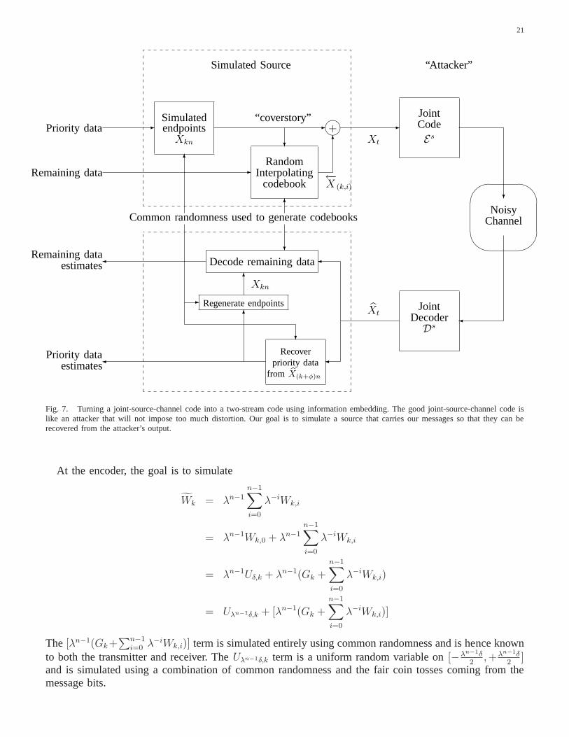
The proof construction is illustrated in Fig. 7. Two messagestreams need to be embedded — a prioritystream that requires anytime reliability and a remaining stream for which Shannon-reliability is goodenough. The priority stream is used to generate the endpoints while the the history part is filled in withthe appropriate conditional distribution. This simulatedprocess is then run through the joint source-channelencoderEs to generate channel inputs. The channel outputs are given tothe joint source-channel decoderDs which produces, after some delayφ, a fidelity d reconstruction of the simulated unstable process. Bylooking at the reconstructions corresponding to the endpoints, it is possible to recover the priority messagebits in an anytime reliable fashion. With these in hand, the remaining stream can also be extracted fromthe historical reconstructions.

A. Necessity of anytime reliability

We follow the spirit of information embedding[34] except that we have noa-priori covertext. Instead weuse a simulated unstable process that uses common randomness and without loss of generality, messagebits assumed to be from iid coin tosses. If the message bits were not fair coin tosses to begin with, XORthem with a one-time pad using common randomness before embedding them. This section parallels thenecessity story in [5], except that in this context, there isthe additional complication of having a specifieddistribution for theWt, not just a bound on the allowed|Wt|.

The result is proved in stages. First, we assume that the density of W is a continuous uniform randomvariable plus something independent. After that, this assumption is relaxed to having a Riemann-integrabledensityfW .

1) Uniform driving noise:Lemma 6.1:Assume the driving noiseW = G + Uδ whereG,Uδ are independent random variables

with Uδ being a uniform random variable on the interval[− δ2,+ δ

2] for someδ > 0.

If a joint source-channel encoder/decoder pair exists for the endpoint process given by (11) that achieves(7) for every positionkn, then for every rational rateR = nR

n< log2 λ, there exists a randomized anytime

code for the channel that achieves an anytime reliability ofα = η log2 λ.

Proof: The goal is to simulate the the endpoint process using the message bits and then to recover themessage bits from the reconstructions of the endpoints. Pick the initial conditionX0 using commonrandomness so it can be ignored in what follows.

21

'

&

$

%

--

?

6

.

“coverstory”Simulated

Xt

+

JointCodeendpoints

Random

codebook

Simulated Source “Attacker”

ChannelNoisy

JointDecoder

?

6

6

-

-

?

6

-

?

6

Interpolating

Common randomness used to generate codebooks

Remaining data

Priority data

Recoverpriority data

Regenerate endpoints

Decode remaining dataRemaining data

Priority data

estimates

estimates

Xkn

←−X (k,i)

Xkn Es

Xt

from X(k+φ)n

Ds

Fig. 7. Turning a joint-source-channel code into a two-stream code using information embedding. The good joint-source-channel code islike an attacker that will not impose too much distortion. Our goal is to simulate asource that carries our messages so that they can berecovered from the attacker’s output.

At the encoder, the goal is to simulate

Wk = λn−1

n−1∑

i=0

λ−iWk,i

= λn−1Wk,0 + λn−1

n−1∑

i=0

λ−iWk,i

= λn−1Uδ,k + λn−1(Gk +n−1∑

i=0

λ−iWk,i)

= Uλn−1δ,k + [λn−1(Gk +n−1∑

i=0

λ−iWk,i)]

The [λn−1(Gk+∑n−1

i=0 λ−iWk,i)] term is simulated entirely using common randomness and is hence known

to both the transmitter and receiver. TheUλn−1δ,k term is a uniform random variable on[−λn−1δ2,+λn−1δ

2]

and is simulated using a combination of common randomness and the fair coin tosses coming from themessage bits.

22

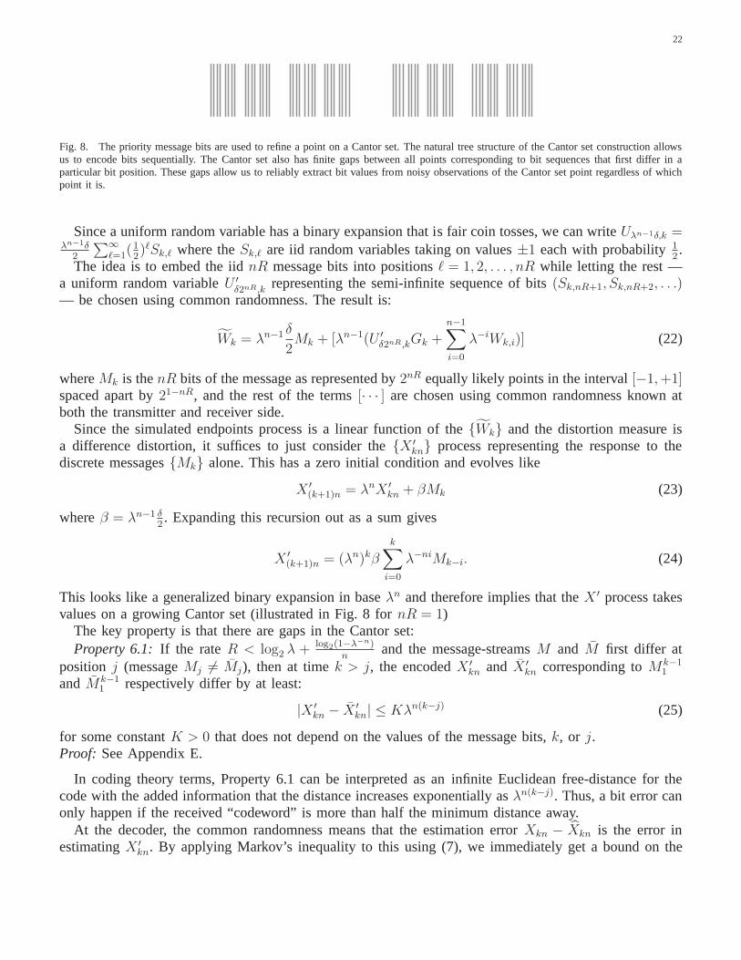
Fig. 8. The priority message bits are used to refine a point on a Cantor set.The natural tree structure of the Cantor set construction allowsus to encode bits sequentially. The Cantor set also has finite gaps between all points corresponding to bit sequences that first differ in aparticular bit position. These gaps allow us to reliably extract bit values from noisy observations of the Cantor set point regardless of whichpoint it is.

Since a uniform random variable has a binary expansion that is fair coin tosses, we can writeUλn−1δ,k =λn−1δ

2

∑∞ℓ=1(

12)ℓSk,ℓ where theSk,ℓ are iid random variables taking on values±1 each with probability1

2.

The idea is to embed the iidnR message bits into positionsℓ = 1, 2, . . . , nR while letting the rest —a uniform random variableU ′

δ2nR,krepresenting the semi-infinite sequence of bits(Sk,nR+1, Sk,nR+2, . . .)

— be chosen using common randomness. The result is:

Wk = λn−1 δ

2Mk + [λn−1(U ′δ2nR,kGk +

n−1∑

i=0

λ−iWk,i)] (22)

whereMk is thenR bits of the message as represented by2nR equally likely points in the interval[−1,+1]spaced apart by21−nR, and the rest of the terms[· · · ] are chosen using common randomness known atboth the transmitter and receiver side.

Since the simulated endpoints process is a linear function of the Wk and the distortion measure isa difference distortion, it suffices to just consider theX ′kn process representing the response to thediscrete messagesMk alone. This has a zero initial condition and evolves like

X ′(k+1)n = λnX ′kn + βMk (23)

whereβ = λn−1 δ2. Expanding this recursion out as a sum gives

X ′(k+1)n = (λn)kβk∑

i=0

λ−niMk−i. (24)

This looks like a generalized binary expansion in baseλn and therefore implies that theX ′ process takesvalues on a growing Cantor set (illustrated in Fig. 8 fornR = 1)

The key property is that there are gaps in the Cantor set:Property 6.1: If the rateR < log2 λ + log2(1−λ−n)

nand the message-streamsM and M first differ at

position j (messageMj 6= Mj), then at timek > j, the encodedX ′kn and X ′kn corresponding toMk−11

andMk−11 respectively differ by at least:

|X ′kn − X′kn| ≤ Kλn(k−j) (25)

for some constantK > 0 that does not depend on the values of the message bits,k, or j.Proof: See Appendix E.

In coding theory terms, Property 6.1 can be interpreted as aninfinite Euclidean free-distance for thecode with the added information that the distance increasesexponentially asλn(k−j). Thus, a bit error canonly happen if the received “codeword” is more than half the minimum distance away.

At the decoder, the common randomness means that the estimation errorXkn − Xkn is the error inestimatingX ′kn. By applying Markov’s inequality to this using (7), we immediately get a bound on the

23

probability of an error on the prefixM i0 for i < k:

P(M i1(kn) 6= M i

1) ≤ P(|X ′kn −X′kn| >

K

2λn(k−i))

= P(|Xkn −Xkn| >K

2λn(k−i))

= P(|Xkn −Xkn|η > (

K

2)η(λn(k−i))η

≤ d(K

2)−η(λn(k−i))η

= K ′2−(η log2 λ)n(k−i).

But n(k− i) is the delay that is experienced at thenR-bit message level. If bits have to be buffered-up toform messages, then the delay at the bit level includes another constantn. This only increases the constantK ′ further but does not change the exponent with large delays. Thus, the desired anytime reliability isobtained.

2) General driving noise:Lemma 6.1 can have the technical smoothness condition weakened to simplyrequiring a Riemann-integrable density for the whiteW driving process.

Lemma 6.2:Assume the driving noiseW has a Riemann-integrable densityfW . If there exists a familyof joint source-channel encoder/decoder pairs for a sequence of increasingn-endpoint problems givenby (11) that achieve (7) for every positionkn, then for every rateR < log2 λ and anytime reliabilityα < η log2 λ, there exists a randomized anytime code for the underlying channel.

Proof: Since the density is Riemann-integrable, Lemma 4.1 applies. Chooseδ such thatγ < λ−2ηn.When simulatingWk,0 in the endpoint process, use common randomness forCγ andW ′′

δ , and follow theprocedure from the proof of Lemma 6.1 forGδ andUδ.

We can thus interpret a “heads” forCγ as an “erasure” with probabilityγ since no message can beencoded in that time period. From the point of view of Lemma 6.1, this can be considered a known nullmessage.

Since the outcome of these coin tosses come from common randomness, the position of these erasuresare known to both the transmitter and the receiver. In this way, it behaves like a packet erasure channelwith feedback. This problem is studied in Theorem 3.3 of [7],and the delay-optimal coding strategyrelative to the erasure channel is to place incoming packetsinto a FIFO queue awaiting a non-erasedopportunity for transmission. The following lemma summarizes the results needed from [7].

Lemma 6.3:Suppose packets arrive deterministically at a rate ofR packets per unit time and enter aFIFO queue drained at constant rate1 per unit time.• Supposeγ < 1

16. If each packet has a size distribution that is bounded belowa geometric(1 − γ)

(i.e. P(Size> s) ≤ γs for all non-negative integerss), then the random delayφ experienced byany individual packet from arrival to departure from the queue satisfiesP(φ > s) ≤ K2−αs for allnon-negatives and some constantK that does not depend ons. Furthermore, ifR < 1

1+2rfor some

r > 0, thenα ≥ − log2 γ − 2γr.• Assume the rateR = 1

nand each packet has a size distribution that is bounded by:P(Size> n(1−

ǫ) + s) ≤ γs for all non-negative integerss. Then the delayφ experienced by any individual packethas a tail distribution bounded in the same way as forR′ = 1

nǫand packets with geometric(1 − γ)

size. That isP(φ > s) ≤ K2−αs whereα ≥ − log2 γ − 2γnǫ−1

2 .Proof: See Theorem 3.3 and Corollary 6.1 of [7].

For our problem, the message bits are arriving deterministically at bit-rateR < log2 λ per unit timeto the transmitter. Pickr > 0 small enough so thatR′ = (1 + 3r)R < log2 λ. Group message bits intopackets of sizenR′. These packets arrive deterministically at rate1

1+3r< 1

1+2rpackets pern time units.

24

Thus, Lemma 6.3 applies and the delay (inn units) experienced by a packet in the queue has a delayerror exponentα of least

− log2 γ − 2γr ≥ − log2 λ−2ηn − 2λ−2ηnr

= n2η log2 λ− 2λ−2ηnr

per n time steps or2η log2 λ−2λ−2ηnr

nper unit time step. Whenn is large, this exponent is much faster

than the delay exponent ofη log2 λ obtained in the proof of Lemma 6.1. The two delays experienced bya bit are independent by construction. Thus, the dominant delay-exponent remainsη log2 λ as desired.

Notice that the simulated endpoint process depends only on common randomness and the messagepackets. Since the common randomness is known perfectly at the receiver by assumption and the messagepackets are known with a probability that tends to1 with delay, the endpoint process is also known withzero distortion with a probability tending to1 as the delay increases.

B. Embedding classical bits

All that remains is to embed the classical message bits into the historical process. The overall construc-tion is described in Fig. 7. First,n is chosen to be large enough so that theR1 stream can be successfullyembedded in the endpoint process by Lemma 6.2.

Now, n is further increased so thatR2 < R←−X |←−X0n (d) the conditional rate-distortion function for the

history given the endpoint. This can be done sincelimn→∞R←−X |←−X0n (d) = RX

∞(d)− log2 λ by Theorem 2.4.By choosing an appropriate additional delay, Lemma 6.2 assures us that the receiver will know all the

past high-priority messages and hence simulated endpointscorrectly with an arbitrarily small probabilityof error ǫ. As described in Section IV-A, this means we now have a familyof systems (indexed bym)that solve the conditional history problem. The condition (8) translates into

limm→∞

supτ≥0P(

1

m

τ+m−1∑

k=τ

1

n

n−1∑

i=1

|←−X (k,i) − X

−(k,i)|

η > d) = 0. (26)

It tells us that by pickingm large enough, the probability of having excess distortion can be made assmall as desired.

The simulatedZk containing the high-priority messages are interpreted as the “coverstory” that mustbe respected when embedding messages into the ~X−k process. TheZk are iid by construction andhence Theorem 3 from [18] (full proofs in [19]) applies and tells us that a lengthm′ > m randomcode with ~X−k drawn independently of each other, but conditional on the iid Zk, can be used to embed

information at any ratenR2 < nR←−X |Zn (d + ǫ) = nR

X|Xnn (d + ǫ) per vector symbol with arbitrarily low

probability of error.

The “weak law of large numbers”-like condition (8), or something like it, is required for the theoremto hold since there are joint source-channel codes for whichmutual information cannot be turned into thereliable communication of bits at arbitrarily low probabilities of error. Consider the following contrivedexample. Suppose there are two different joint source-channel codes available: one has a target distortionof d1 and the other has a target distortion ofd2 = 10d1. The actual joint code, which is presumed to haveaccess to common randomness, could decide with probability1

1000to use the second code rather than the

first. In such a case, the ensemble average mutual information is close toR(d1) − log2 λ bits, but withnon-vanishing probability 1

1000we might not be able sustain such a rate over the virtual channel.

We conjecture that for DMCs, if any joint source-channel codeexists that hits the target distortion onaverage, then one should also exist that meets (8) and it should be possible to simultaneously communicatetwo streams of messages reliably with anytime reliability on the first stream and enough residual rate onthe second.

25

VII. U NSTABLE GAUSS-MARKOV PROCESSES WITH SQUARED-ERROR DISTORTION

A. Source-coding for Gaussian processes

The goal here is to prove Corollary 2.1. The strategy is essentially as before. One simplification isthat we can make full use of Theorem 2.4 and rely onR

←−X∞(d) = RX

∞(d) − log2 λ. There is thus no rateloss in encoding the historical segments on a block-by-block basis rather than using superblocks andconditional encodings. The only issue that remains is dealing with the unbounded support when encodingthe checkpoints.

The overall approach is: (key differencesitalicized)(a) Look at time in blocks of sizen and encode the values of checkpointsXkn recursively to very high

precision using a prefix-freevariable-lengthcode with raten(log2 λ+ ǫ1) +Lk bits per value, wheretheLk are iid random variables with appropriately nice properties.

(b) Smooth out the variable-length code by running it through a FIFO queue drained at constant rateR1 = log2 λ+ ǫ1 + ǫq. Make sure that the delay exponent in the queue is high enough.

(c) Use theexact valuefor the ending checkpointX(k+1)n (instead of the quantizedX) to transform thesegment immediately before it so that it looks exactly like astable backwards Gaussian process oflength n with initial condition 0. Encode each block of the backwards history process to average-fidelity d using a fixed-rate rate-distortion code for the backwards process that operates at rateR

←−X∞(d)+

ǫs.(d) At the decoder, waitφ time units and attempt to decode the checkpoints to high fidelity. If the FIFO

queue is running too far behind, then extrapolate a reconstruction based on the last fully decodedcheckpoint.

(e) Decode the history process to average-fidelityd and combine it with the recursively quantizedcheckpoints to get the reconstruction.a) Encoding the checkpoints:(11) remains valid, but the termWk = λn−1

∑n−1i=0 λ

−iWkn+i is notbounded since theWi are iid Gaussians. TheWk are instead Gaussian with variance

σ2 = λ2(n−1)

n−1∑

i=0

λ−2iσ2

≤ λ2(n−1)σ2

∞∑

i=0

λ−2i

= λ2n σ2

λ2 − 1.

The standard deviationσ is thereforeλn σ√λ2−1

. Pick l = 2ǫ13n and essentially pretend that this random

variableWk has bounded support oflσ during the encoding process. By comparing (12) to the above,the

effectiveΩ is simply lσ 2(λ−1)√λ2−1

= 2ǫ13nσ√

λ−1λ+1

. DefineΩ = σ√

λ−1λ+1

so that the effectiveΩ = 2ǫ13nΩ.

Encode the checkpoint increments recursively as before, only add an additional variable-length codefor the value of⌊

fWleσ + 1

2⌋ while treating the remainder using the fixed-rate code as before. The variable

length code is a unary encoding that counts how manylσ away from the center theWk actually is. (Fig. 9illustrates the unary code.) LetLk be the length of thek-th unary codeword. This is bounded above by

P (Lk ≥ 3 + j) = P (|W | > jlσ).

Let N be a standard Gaussian random variable and rewrite this as

P (Lk ≥ 3 + j) = P (|N | > j2ǫ13n) ≤ exp(−

1

2j22

2ǫ13n) (27)

and soLk is very likely indeed to be small and certainly has a finite expectationL < 4 if n is large.

26

Offset Codeword0 100

+1 1110-1 1100+2 11110-2 11010+3 111110-3 110110+4 1111110-4 1101110...

...

Fig. 9. Unary encoding of integer offsets to deal with the unbounded support. The first bit denotes start while the nest two bits reflectthe sign. The length of the rest reflects the magnitude of the offset with a zero termination. The encoding is prefix-free and hence uniquelydecodable. The length of the encoding of integerS is bounded by3 + |S|

The fixed-rate part of the checkpoint encoding has a rate thatis the same as that given by (13), exceptthat Ω is now mildly a function ofn. Plugging in2

ǫ13nΩ for Ω in (13) gives

R1,f ≥ max

(log2 λ+

log2(1 + Ω∆(λ−1)

) + log2(2 + Ω∆

)

n,log2⌈

Ω0

∆⌉

n

)

= max

log2 λ+

log2(1 + 2ǫ13 n eΩ

∆(λ−1)) + log2(2 + 2

ǫ13 n eΩ∆

)

n,log2⌈

Ω0

∆⌉

n

= max

log2 λ+

2

3ǫ1 +

log2(2− ǫ1

3n +

eΩ∆(λ−1)

) + log2(21− ǫ1

3n +

eΩ∆

)

n,log2⌈

Ω0

∆⌉

n

.

Essentially, the required rateR1,f for the fixed-rate part has only increased by a small constant23ǫ1.

Holding ∆ fixed and assumingn is large enough, we can see that

R1,f = log2 λ+ ǫ1 (28)

is sufficient.b) Smoothing out the flow:The code so far is variable-rate and to turn this into a fixed-rateR1 =

log2 λ+ ǫ1 + ǫq bitstream, it is smoothed by going through a FIFO queue. First, encode the offset usingthe variable-length code and then recursively encode the increment as was done in the finite support case.All such codes will begin with a1 and thus we can use zeros to pad the end of a codeword wheneverthe FIFO is empty. Whenn is large, the average input rate to the FIFO is smaller than the output rateand hence it will be empty infinitely often.

c) Getting history and encoding it:Section IV explains why such a transformation is possible bysubtracting off a scaled version of the endpoint. The resultis a stable Gaussian process and so [9] revealsthat it can be encoded arbitrarily close to its rate-distortion boundR

←−X∞(d) = RX

∞(d)− log2 λ if n is largeenough.

d) Decoding the checkpoints:The decoder can wait long enough so that the checkpoint we areinterested in is very likely to have made it through the FIFO queue by now. The ideas here are similarto [7], [35] in that a FIFO queue is used to smooth out the rate variation with good large deviationsperformance. There isnǫq slack that has to accommodateLk bits. Becausen can be made large, the errorexponent with delay here can be made as large as needed.

27

More precisely, a packet of sizen(ǫ1 +log2 λ)+Lk bits arrives everyn time units where theLk are iid.This is drained at rateR1 = ǫq + ǫ1 + log2 λ. An alternative view is therefore that a point packet arrivesdeterministically everyn time units and it has a random service timeTk given byn ǫ1+log2 λ

ǫq+ǫ1+log2 λ+ Lk

ǫq+ǫ1+log2 λ.

Define(1− ǫ′q) = ǫ1+log2 λ

ǫq+ǫ1+log2 λ. Then the random service timeTk = (1− ǫ′q)n+ Lk

ǫq+ǫ1+log2 λwhen measured

in time units orT bk = (1− ǫ′q)nR1 + Lk when measured in bit-units.This can be analyzed using large-deviations techniques or by applying standard results in queuing. The

important thing is a bound on the lengthLk which is provided by (27). It is clear that1,

P (Lk ≥ 3 + j) ≤ exp(−1

2j22

2ǫ13n)

≤ exp(−22ǫ13n−1)j).

Since an exponential eventually dominates all constants, we know that for anyβ > 0, there exists asufficiently largen so that:

P (Lk − 3 > j) ≤ 2−βj. (29)

Thus, the delay (in bits) experienced by a block in the queue will behave no worse than that of pointmessages arriving everynR1 bits where each requires at leastnR1(1 − ǫ

′q) + 3 = nR1(1 − ǫ

′′q) bits plus

an iid geometric(1− p) number of bits withp = 2−β.Lemma 6.3 applies to this queuing problem and the second partof that lemma tells us that the delay

performance is exactly the same as that of a system with pointmessages arriving everynǫ′′q bits requiring

only an iid geometric number of bits. Since1nǫ′′q

is small, the first part of Lemma 6.3 applies. Setr =nǫ′′q3−1,

then the bit-delay exponentαb is at least

αb ≥ − log2 2−β − 2−βr

= β − 2−β(nǫ′′q3−1)

which is at leastβ − 1 whennǫ′′q ≥ 3. Converting between bit-delay and time-delay is essentially just afactor of log2 λ and so the time-delay exponent is at leastβ−1

log2 λ. But β can be made as large as we want

by choosingn large enough.e) Getting the final reconstruction:The history process is added to the recovered checkpoint. This

differs from the original process by only the error in the history plus the impact of the error in thecheckpoint. The checkpoint reconstruction-error’s impact dies exponentially since the history process isstable. So the target distortion is achieved if the checkpoint has arrived by the time reconstruction isattempted. By choosing a large enough end-to-end delayφ, the probability of this can be made as highas we like.

However, the goal is not just to meet the target distortion level d with high probability, it is also to hitthe target in expectation. Thus, we must bound the impact of not having the checkpoint available in time.When this happens, the un-interpretable history information is ignored and the most recent checkpoint issimply extrapolated forward to the current time. The expected squared errors grow asλ2ψ whereψ is thedelay in time-units. The arguments here exactly parallel those of Theorem 2.2, where the FIFO queue isacting like an anytime code. Since the delay-exponent of thequeue is as large as we want, it can be madelarger than2 log2 λ. Thus, the expected distortion coming from such “overflow” situations is as small asdesired. This completes the proof of Corollary 2.1.

1While this proof is written for the Gaussian case, the arguments here readilygeneralize to any driving distributionW that has at leastan exponential tail probability. To accommodateW with power-law tail distributions would require the use of logarithmic encodings asdescribed in [36], [37]. This does not work for our case because the unary nature of the encoding is important when we consider transportingsuch bitstreams across a noisy channel.

28

B. Channel sufficiency for communicating Gaussian processes

This section shows why Corollary 2.2 is true. The story in the Gaussian case is mostly unchanged sincethe historical information is as classical as ever. The onlyissue is with the checkpoint stream. An errorin a bit ψ steps ago can do more than propagate through the usual pathway. It could also damage the bitscorresponding to the variable-length offset.

Because of the unary encoding and the2ǫ13n expansion in the effectiveΩ, an uncorrected bit-stream

errorψ time-steps ago can only impact the error in the checkpoint reconstruction by4ψ(log2 λ)2ǫ13n since

the worst error is clearly to flip the sign bit and keep the unary codeword from terminating thereby makingit at most2ψ log2 λ bits long. The current reconstruction is therefore incorrect by anO(ψ2

ǫ13nλψ) change

in its value. As far asη-distortion is concerned, the distortion grows by a factorO(ψη2ηǫ13nληψ) from what

it would be with correct reconstruction. Asymptotically, the delayψ is much larger than the block-lengthn and so the polynomial term in front is insignificant relativeto the exponential inψ. If the code hasanytime reliabilityα > η log2 λ, then the same argument as Theorem 2.2 applies and the Corollary holds.

VIII. E XTENSIONS TO THE VECTOR CASE

With the scalar case explored, it is natural to consider whathappens for general finite-dimensionallinear models whereλ is replaced with a matrixA andX is a vector. In the Gaussian process case, thesewill correspond to cases with formally rational power-spectral densities. Though the details are left to thereader, the story is sketched here. No fundamentally new phenomena arise in the vector case, except thatdifferent anytime reliabilities can be required on different streams arising from the same source as is seenin the control context [6].

The source-coding results here naturally extend to the fully observed vector case with generic drivingnoise distributions. Instead of two message streams, thereis one special stream for each unstable eigenvalueλi of A and a singe final stream capturing the residual information across all dimensions. All the sufficiencyresults also generalize in a straightforward manner — each of the unstable streams requires a correspondinganytime reliability depending on the distortion function’s η and the magnitude of the eigenvalue. Themultiple priority-stream necessity results also follow generically.2 This is a straightforward applicationof a system diagonalization3 argument followed by an eigenvalue by eigenvalue analysis.The necessityresult for the residual rate follows the same proof as here based on inverse-conditional rate-distortion withthe endpoints in all dimensions used as side-information.

The case of partially observed vector Markov processes where the observationsCy ~X are linear in thesystem state requires one more trick. We need to invoke the observability4 of the system state. Insteadof a single checkpoint pair, use an appropriate number5 of consecutive values for the observation andencode them together to high fidelity∆. This can be done by transforming coordinates linearly so that thesystem is diagonal, though driven by correlated noise, fromcheckpoint-block to the next checkpoint-block.The initial condition is governed by the self-noise that is unavoidable while trying to observe the state.Each unstable eigenvalue will contribute its ownlog2 λi term to the first stream rate and will require theappropriate anytime reliability. The overhead continues to be sublinear inn and the residual informationcontinues to be classical in nature by the same arguments given here.

2The required condition is that the the driving noise distributionW should not have support isolated to an invariant subspace ofA. If thatwere to happen, there would be modes of the process that are never excited.

3The case of non-diagonal Jordan blocks is only a challenge for the necessity part regarding anytime reliability. It is covered in [6] in thecontrol context. The same argument holds here with a Riemann-integrable joint-density assumption on the driving noise.

4The linear observation should not be restricted to a single invariant subspace. If it were, we could drop the other subspaces from themodel as irrelevant to the observed process under consideration.

5The appropriate number is twice the number of observations required before all of the unstable subspaces show up in the observation.This number is bounded above by twice the dimensionality of the vector state space. The factor of two is to allow each block to have itsown beginning and end.

29

The partially observed necessity story is essentially unchanged on the information embedding side,except that every long block should be followed by a miniblock of length equal to the dimensionalityk during which no message is embedded and only common-randomness is used to generate the drivingnoise. This will allow the decoder to easily use observability to get noisy access to the unstable stateitself.

In [6], these techniques are applied in the context of control rather than estimation. The interestedreader is referred there for the details. Some simplifications to the general story might be possible in thecase of SISO autoregressive processes, but we have not explored them in detail.

IX. CONCLUSIONS

We have characterized the nature of information in an unstable Markov process. On the source codingside, this was done by giving the fixed-rate coding Theorem 2.1. This theorem’s code construction naturallyproduces two streams — one that captures the essential unstable nature of the process and requires a rateof at leastlog2 λ, and another that captures the essentially classical nature of the information left over. Thequantitative distortion is dominated by the encoding of thesecond stream, while the first stream servesto ensure its finiteness as time goes on. The essentially stable nature of the second stream’s informationis then made precise by Theorem 2.4 which relates the forwardD(R) curve to the “backwards” onecorresponding to a stable process.

At the intersection of source and channel coding, the notionof anytime reliability was reviewed andTheorem 5.1 shows that it is nonzero for DMCs at rates below capacity. Theorem 2.2 and Lemma 6.2then shows that the first stream requires a high-enough anytime reliability from a communication systemrather than merely enough rate. In contrast, Theorems 2.3 and 2.5 show that the second stream requiresonly sufficient rate. Together, all these results establishthe relevant separation principle for such unstableMarkov processes.

This work brings exponentially unstable processes firmly into the fold of information theory. Morefundamentally, it shows that reliability functions are nota matter purely internal to channel coding. In thecase of unstable processes, the demand for appropriate reliability arises at the source-channel interface.Thus unstable processes have the potential to be useful models while taking an information-theoretic lookat QoS issues in communication systems. The success of the “reductions and equivalences” paradigm of[5], [19] here suggests that this approach might also be useful in understanding other situations in whichclassical approaches to separation theorems break down.

APPENDIX ARIEMANN -INTEGRABLE DENSITIES AS MIXTURES

It is often conceptually useful to think of generic random variables with Riemann-integrable densitiesas being mixtures of a blurred uniform random variable alongwith something else. This appendix provesLemma 4.1.

Since the density is Riemann-integrable,∫ +∞

−∞fW (w)dw = lim

δ→0

+∞∑

i=−∞δ minx∈[iδ− δ

2,iδ+ δ

2]fW (x)

Thus,fW can be expressed as a non-negative piecewise constant function f ′W that only changes everyδ units plus a non-negative functionf ′′W representing the “error” in Riemann-integration from below. Bychoosingδ small enough, the total mass inf ′′W can be made as small as desired since the Riemann sumsabove converge.

Chooseδ such that the total mass inf ′′W is γ. So

fW = (1− γ)(f ′W

1− γ) + γ(

f ′′Wγ

) (30)

30

and thusW can thus be simulated in the following way:1) Flip an independent biased coinCγ with probability of headsγ.2) If heads, independently draw the value ofW from the densityf

′′

W

γcorresponding to a random variable

W ′′.3) If tails, independently draw the value ofW from the random variableW ′′ with piecewise constant

density f ′W1−γ . This can clearly be done by using a discrete random variableGδ plus an independent

uniform random variableUδ so thatW ′′ = Gδ + Uδ has densityf′

W

1−γ .This proves the result.

APPENDIX BENTROPY BOUND FOR QUANTIZED RANDOM VARIABLES WITH BOUNDED MOMENTS

Lemma B.1:Consider a random variableZ that is quantized to precision∆ soZq = Q∆(Z). Furthersuppose thatE[|Z|η] ≤ K whereK > ∆η. Then

H(S) < 7 +log2K

η+ 2 log2

log2K

η+ log2

1

∆+ 2 log2 log2

1

∆+

5 + ln 2

η ln 2. (31)

Proof: Let Zq = S∆ whereS is an integer. Then|S| ≤ 1 + |Z|∆

and so

E[|S|η] ≤ E[(1 +|Z|

∆)η]

≤ E[(2 max

(1,|Z|

∆

))η]

= E[2η max

(1η, (|Z|

∆)η)

]

≤ E[2η + 2η|Z|η

∆η]

= 2η +2η

∆ηE[|Z|η]

≤ 2η +2ηK

∆η

< 2η+1 K

∆η.

Applying the Markov inequality gives

P(|S| ≥ s) ≤ min(1,2η+1K

∆ηs−η). (32)

The integerS can be encoded into bits using a self-punctuated code using less than4 + log2(|S|) +2 log2(1 + log2(|S|+ 1)) bits to encodeS 6= 0 [38]. First encode the sign ofS using a single bit. Thereare at most1 + log2(|S| + 1) digits in the natural binary expansion of|S|. This length can be encodedusing at most2 + 2 log2(1 + log2(|S| + 1)) bits by giving its binary expansion with each digit followedby a 0 if it is not the last digit, and a1 if it is the last digit. Finally,|S| itself can be encoded using atmost1 + log2 |S| bits.

Since the entropy must be less than the expected code-lengthfor any code,

H(S) ≤ 4 + E[log2(|S|)] + 2E[log2(1 + log2(|S|+ 1))]

= 4 +

∫ ∞

0

P(log2(|S|) > l)dl + 2

∫ ∞

0

P(log2(1 + log2(|S|+ 1)) > l)dl.

31

First, we deal with the dominant term∫ ∞

0

P(log2(|S|) > l)dl

=

∫ ∞

0

P(|S| > 2l)dl

≤

∫ ∞

0

min(1,2η+1K

∆η2−ηl)dl

=1

ηlog2(

2η+1K

∆η) +

∫ ∞

0

2−ηudl

= 1 +log2K

η+ log2

1

∆+

1 + ln 2

η ln 2

Next, consider the smaller term

2

∫ ∞

0

P(log2(1 + log2(|S|+ 1)) > l)dl

= 2

∫ ∞

0

P(log2(|S|+ 1) > 2l − 1)dl

= 2

∫ ∞

0

P(|S|+ 1 >22l

2)dl

≤ 2(1 +

∫ ∞

0

P(|S| > 22l

)dl)

≤ 2 + 2

∫ ∞

0

min(1,2η+1K

∆η2−η2

l

)dl

= 2 + 2 log2

log22η+1K

∆η

η+ 2

∫ ∞

0

2−η2l

dl

< 2 + 2 log2

log2K

η+ 2 log2(1 +

1

η) + 2 log2 log2

1

∆+

2

η ln 2

≤ 2 + 2 log2

log2K

η+ 2 log2 log2

1

∆+

4

η ln 2

where the final inequalities come from the concave∩ nature oflog2 and lower bounding2l with just l.Putting everything together gives the desired result.

APPENDIX CPROOF OFPROPOSITION3.2

From (3) and (2), we know for everyǫ2 > 0, if ∆ is small enough andn is large enough, that thereexists a random vectorY n−1

0 so that 1n

∑n−1i=0 ρ(Xi, Yi) = d + ǫ3 and that even the best such vector must

satisfyn(RX

∞(d)− ǫ2) ≤ I(Xn−10 ;Y n−1

0 ) ≤ n(RX∞(d) + ǫ2).

Decompose the relevant mutual information as

I(Xn−10 ;Y n−1

0 |Zq,Θ) = −I(Xn−10 ;Zq|Θ) + I(Xn−1

0 ;Y n−10 , Zq|Θ). (33)

To get the desired result of asymptotic equality, this conditional mutual information has to be both upperand lower bounded. To upper bound the conditional mutual information, we lower boundI(Xn−1

0 ;Zq|Θ)and upper boundI(Xn−1

0 ;Y n−10 , Zq|Θ). Vice-versa to get the lower bound.

32

A. Lower boundingI(Xn−10 ;Zq|Θ)

The first term is easily lower bounded for∆ small enough since

I(Xn−10 ;Zq|Θ) = H(Zq|Θ)−H(Zq|Xn

1 ,Θ)

= H(Zq|Θ)

≥ H(Zq|Θ,W n−20 )

≥ ⌊log2 λn−1⌋

= ⌊(n− 1) log2 λ⌋. (34)

This holds since conditioned on the final ditherΘ, the quantized endpoint is a discrete random variablethat is a deterministic function ofXn−1 and conditioning reduces entropy. ButZq conditioned on thedriving noiseW n−2

0 is just the∆-precision quantization ofλn−1 times a uniform random variable ofwidth ∆ and hence has discrete entropy≥ log2 λ

n−1.

B. Upper boundingI(Xn−10 ;Zq|Θ)

To upper-bound this term, Lemma B.1 can be used to see

I(Xn−10 ;Zq|Θ) = H(Zq|Θ)

< 7 +log2K

′

η+ 2 log2

log2K′

η+ log2

1

∆+ 2 log2 log2

1

∆+

5 + ln 2

η ln 2(35)

whereK ′ is an upper-bound toE[|Z|η]. Such an upper-bound is readily available since

E[|Z|η] = E[|Xn|η]

≤ E[(∆

2+ |∑

i=0

n− 1λn−1−iWi|)η]

= E[(∆

2+ λn−1|

∑

i=0

n− 1λ−iWi|)η]

= λη(n−1)E[(∆

2λn−1+ |∑

i=0

n− 1λ−iWi|)η]

≤ λη(n−1)E[(2 max(∆

2λn−1, |∑

i=0

n− 1λ−iWi|)η]

< λη(n−1)(∆η

λη(n−1)+ 2ηK).

Using this forK ′ and taking logs shows

log2K′

η=

log2(λη(n−1)( ∆η

λη(n−1) + 2ηK))

η

= 1 + (n− 1) log2 λ+log2(

∆η

λη(n−1) + 2ηK)

η

Substituting this in gives the desired bound

I(Xn−10 ;Zq|Θ)

< 8 + (n− 1) log2 λ+ 2 log2(1 + (n− 1) log2 λ+log2(

∆η

λη(n−1) + 2ηK)

η) + log2

1

∆+ 2 log2 log2

1

∆+

5 + ln 2

η ln 2.(36)

There is only a singleO(n) term above, and it is(n− 1) log2 λ. Everything else iso(n).

33

C. Lower boundingI(Xn−10 ;Y n−1

0 , Zq|Θ)

We need to establishI(Xn−1

0 ;Y n−10 , Zq|Θ) ≥ n(RX

∞(d)− ǫ2). (37)

This is immediately obvious from

I(Xn−10 ;Y n−1

0 , Zq|Θ) = I(Xn−10 ;Y n−1

0 |Θ) +H(Zq|Θ, Y n−10 )−H(Zq|Θ, Y n−1

0 , Xn−10 )

= I(Xn−10 ;Y n−1

0 |Θ) +H(Zq|Θ, Y n−10 )

≥ n(RX∞(d)− ǫ2).

The first equality is just expanding the mutual information and recognizing the fact thatZq is discrete onceconditioned on the ditherΘ and soH is the regular discrete entropy here. LetQ(∆,Θ) denote the ditheredscalar quantizer used to generate the encoded checkpoints,just appropriately translated so it can apply tothe X giving Zq = Q(∆,Θ)(Xn−1). The next equality is a consequence of this deterministic relationship.Finally, the discrete entropy is always positive and can be dropped to give a lower bound.

D. Upper boundingI(Xn−10 ;Y n−1

0 , Zq|Θ)

The second term of (33) is upper bounded in a way similar to thefirst term. We need to establish

I(Xn−10 ;Y n−1

0 , Zq|Θ) ≤ n(RX∞(d) + ǫ2) + o(n). (38)

Expand the mutual information as before

I(Xn−10 ;Y n−1

0 , Zq|Θ) = I(Xn−10 ;Y n−1

0 |Θ) +H(Zq|Θ, Y n−10 )

≤ I(Xn−10 ;Y n−1

0 |Θ) +H(Zq|Θ, Yn−1)

= n(RX∞(d) + ǫ2) +H(Zq −Q(∆,Θ)(Yn−1)|Θ, Yn−1)

≤ n(RX∞(d) + ǫ2) + log2 3 +H(Q(∆,Θ)(Xn−1 − Yn−1)|Θ).

The first inequality comes from dropping conditioning. After that, the quantizerQ(∆,Θ) can be appliedto Yn−1 so thatZq − Q(∆,Θ)(Yn−1) = S∆ whereS is an integer-valued random variable representinghow many steps up or down the∆-quantization ladder are needed to get fromQ(∆,Θ)(Yn−1) to Zq. Thedifference of two quantized numbers differs by at most 1 quantization bin from the quantization of thedifference. This slack of up to 1 bin in either direction can be encoded usinglog2 3 bits.

At this point, Lemma B.1 applies using the trivial upper bound n(d + ǫ3) for the η-th moment ofXn−1 − Yn−1, since the worst case is for the entire distortion to fall on the last component of the vector.

H(Q(∆,Θ)(Xn−1 − Yn−1)|Θ)

< 7 +log2 n(d+ ǫ3)

η+ 2 log2

log2 n(d+ ǫ2)

η+ log2

1

∆+ 2 log2 log2

1

∆+

5 + ln 2

η ln 2

The log2 n term is certainlyo(n). The only other term that might raise concern islog21∆

, but that iso(n) since (13) tells us that we are already required to choosen much larger than that to haveR1 closeto log2 λ in the first stream. The order of limits is to always letn go to infinity before∆ goes to zero.

E. Putting pieces together

With (38) established, it can be applied along with (34) to (33) and gives

I(Xn−10 ;Y n−1

0 |Zq,Θ) ≤ n(RX∞(d)− log2 λ+ ǫ2) + o(n). (39)

Taking n to∞ and dividing through byn establishes the desired result on the upper bound.Similarly putting together (36) and (37) gives

I(Xn−10 ;Y n−1

0 |Zq,Θ) ≥ n(RX∞(d)− log2 λ− ǫ2)− o(n). (40)

Taking n to∞ and dividing through byn establishes the desired result on the lower bound.But ǫ2 was arbitrary and this establishes the desired result.

34

APPENDIX DPROOF OFTHEOREM 5.1

Interpret the random ensemble of infinite tree codes as a single code with both encoder and decoderhaving access to the common-randomness used to generate thecode-tree. Populate the tree with iid channelinputs drawn from the distribution that achievesEr(R) for block codes. Theorem 7 in [26] tells us thatthe code achieves anytime reliabilityα = Er(R) since the analysis uses the same infinite ensemble forall i and delays.

Alternatively, this can be seen from first principles for ML decoding by observing that any false pathBi

1 can be divided into a true prefixBj−11 and a false suffixBi

j. The iid nature of the channel inputson the code tree tells us that the true code-suffix corresponding to the received channel outputs fromtime j

Rto t is independent of any false code-suffix. Since there are≤ 2R(t− j

R) such false code-suffixes

(ignoring integer effects) at depthj, Gallager’s random block-coding analysis from [8] appliessince allthat it requires is pairwise independence between true and false codewords.

P(Bj(t) 6= Bj|Bj−11 already known)

≤ P(error on random code with2R(t− jR

) words and block lengtht− ⌈j

R⌉)

≤ 2−(t−⌈ jR⌉)Er(R)

≤ 2−(t− jR−1)Er(R)

The probability of error onBi1 can be bounded by the union bound overj = 1 . . . i.

P(Bi1(t) 6= Bi

1) ≤i∑

j=1

P(Bj(t) 6= Bj|Bj−11 already known)

≤i∑

j=1

2−(t− jR−1)Er(R)

<

∞∑

j=0

2−(t− iR−j−1)Er(R)

= K2−(t− iR

)Er(R)

The exponent for the probability of error is dominated by theshortest codeword length in the union bound,and this corresponds tot− i

R.

APPENDIX EPROOF OFPROPERTY6.1

|X ′kn − X′kn| ≥ λn(k−j)β(|Mj − Mj| −

∣∣∣∣∣

∞∑

i=j+1

λ−n(i−j)(Mi − Mi)

∣∣∣∣∣)

≥ λn(k−j)β(|Mj − Mj| − 2λ−n∞∑

i=0

λ−ni)

≥ λn(k−j)β(21−nR − 2λ−n

1− λ−n)

= λn(k−j)2β(2−nR −1

λn − 1)

which is positive as long as2−nR > 1λn−1

or nR < log2(λn−1). We can thus useK = 2β(2−nR− 1

λn−1) =

δλ(2n(log2 λ−R) − λn

λn−1) and the property is proved.

35

ACKNOWLEDGMENTS

The authors would like to give special thanks to Mukul Agarwal for the discussions regarding this paperand the resulting contributions in [19] where one of the key results required is proved. We also thankNigel Newton, Nicola Elia, and Sekhar Tatikonda for severalconstructive discussions about this generalsubject over a long period of time which have influenced this work in important ways.

REFERENCES

[1] C. E. Shannon, “A mathematical theory of communication,”Bell System Technical Journal, vol. 27, pp. 379–423, 623–656, Jul./Oct.1948.

[2] ——, “Coding theorems for a discrete source with a fidelity criterion,”IRE National Convention Record, vol. 7, no. 4, pp. 142–163,1959.

[3] S. Vembu, S. Verdu, and Y. Steinberg, “The source-channel separation theorem revisited,”IEEE Trans. Inf. Theory, vol. 41, no. 1, pp.44–54, Jan. 1995.

[4] A. Ephremides and B. Hajek, “Information theory and communication networks: An unconsummated union,”IEEE Trans. Inf. Theory,vol. 44, pp. 2416–2434, Oct. 1998.

[5] A. Sahai and S. K. Mitter, “The necessity and sufficiency of anytimecapacity for stabilization of a linear system over a noisycommunication link. part I: scalar systems,”IEEE Trans. Inf. Theory, vol. 52, no. 8, pp. 3369–3395, Aug. 2006.

[6] ——, “The necessity and sufficiency of anytime capacity for stabilization of a linear system over a noisycommunication link. part II: vector systems,”IEEE Trans. Inf. Theory, submitted for publication. [Online]. Available:http://www.eecs.berkeley.edu/˜sahai/Papers/control-part-II.pdf

[7] A. Sahai, “Why block-length and delay behave differently if feedback is present,”IEEE Trans. Inf. Theory, Submitted. [Online].Available: http://www.eecs.berkeley.edu/˜sahai/Papers/FocusingBound.pdf

[8] R. G. Gallager,Information Theory and Reliable Communication. New York, NY: John Wiley, 1971.[9] R. Gray, “Information rates of autoregressive processes,”IEEE Trans. Inf. Theory, vol. 16, no. 4, pp. 412–421, Jul. 1970.

[10] T. Hashimoto and S. Arimoto, “On the rate-distortion function for the nonstationary autoregressive process,”IEEE Trans. Inf. Theory,vol. 26, no. 4, pp. 478–480, Apr. 1980.

[11] T. Berger, “Information rates of Wiener processes,”IEEE Trans. Inf. Theory, vol. 16, no. 2, pp. 134–139, Mar. 1970.[12] ——, Rate Distortion Theory. Englewood Cliffs, NJ: Prentice-Hall, 1971.[13] A. Sahai, “A variable rate source-coding theorem for unstable scalar markov processes,” inProceedings of the 2001 IEEE Symposium

on Information Theory, Washington, DC, Jun. 2001.[14] ——, “Any-time information theory,” Ph.D. dissertation, Massachusetts Institute of Technology, Cambridge, MA, 2001.[15] S. K. Mitter and N. J. Newton, “Information flow and entropy production in the Kalman-Bucy filter,”Journal of Statistical Physics,

vol. 118, no. 1, pp. 145–175, Jan. 2005.[16] A. Sahai and S. K. Mitter, “A fundamental need for differentiated‘quality of service’ over communication links: An information

theoretic approach,” inProceedings of the Allerton Conference on Communication, Control, and Computing, Monticello, IL, Oct. 2000.[17] J. E. Hopcroft and J. D. Ullman,Introduction to Automata Theory, Languages, and Computation. Reading, MA: Addison-Wesley,

1979.[18] M. Agarwal, A. Sahai, and S. K. Mitter, “Coding into a source: A direct inverse rate-distortion theorem,” inProceedings of the Allerton

Conference on Communication, Control, and Computing, Monticello, IL, Sep. 2006.[19] ——, “A direct equivalence perspective on the separation theorem,” IEEE Trans. Inf. Theory, In preparation.[20] B. Rimoldi, “Successive refinement of information: Characterization of the achievable rates,”IEEE Trans. Inf. Theory, vol. 40, no. 1,

pp. 253–259, Jan. 1994.[21] S. Verdu and T. S. Han, “A general formula for channel capacity,” IEEE Trans. Inf. Theory, vol. 40, no. 4, pp. 1147–1157, Jul. 1994.[22] S. Tatikonda, “Control under communication constraints,” Ph.D.dissertation, Massachusetts Institute of Technology, Cambridge, MA,

2000.[23] S. Tatikonda, A. Sahai, and S. K. Mitter, “Stochastic linear control over a communication channel,”IEEE Trans. Autom. Control,

vol. 49, no. 9, pp. 1549–1561, Sep. 2004.[24] R. Zamir and M. Feder, “On universal quantization by randomized uniform/lattice quantizers,”IEEE Trans. Inf. Theory, vol. 38, no. 2,

pp. 428–436, Mar. 1992.[25] B. M. Leiner and R. M. Gray, “Rate-distortion theory for ergodic sources with side information,”IEEE Trans. Inf. Theory, vol. 20,

no. 5, pp. 672–675, Sep. 1974.[26] G. D. Forney, “Convolutional codes II. maximum-likelihood decoding,” Information and Control, vol. 25, no. 3, pp. 222–266, Jul.

1974.[27] ——, “Convolutional codes III. sequential decoding,”Information and Control, vol. 25, no. 3, pp. 267–297, Jul. 1974.[28] F. Jelinek, “Upper bounds on sequential decoding performance parameters,”IEEE Trans. Inf. Theory, vol. 20, no. 2, pp. 227–239, Mar.

1974.[29] M. S. Pinsker, “Bounds on the probability and of the number of correctable errors for nonblock codes,”Problemy Peredachi Informatsii,

vol. 3, no. 4, pp. 44–55, Oct./Dec. 1967.[30] A. Sahai and T. Simsek, “On the variable-delay reliability function ofdiscrete memoryless channels with access to noisy feedback,”

in Proceedings of the IEEE Workshop on Information Theory, San Antonio, TX, Nov. 2004.[31] S. Draper and A. Sahai, “Noisy feedback improves communication reliability,” in Proc. IEEE International Symposium on Information

Theory, Jul. 2006. [Online]. Available: http://www.eecs.berkeley.edu/˜sahai/Papers/DraperSahaiISIT06.pdf[32] ——, “Variable-length coding with noisy feedback,”European Transactions on Telecommunications, Submitted.

36

[33] Y. Liang, A. Goldsmith, and M. Effros, “Distortion metrics of composite channels with receiver side information,” inProceedings ofthe 2007 Information Theory Workshop, Sep. 2007, pp. 559–564.

[34] P. Moulin and J. A. O’Sullivan, “Information-theoretic analysis ofinformation hiding,” IEEE Trans. Inf. Theory, vol. 49, no. 3, pp.563–593, Mar. 2003.

[35] A. Sahai and S. K. Mitter, “Source coding and channel requirements for unstable processes,”IEEE Trans. Inf. Theory, Submitted,2006. [Online]. Available: http://www.eecs.berkeley.edu/˜sahai/Papers/anytime.pdf

[36] G. N. Nair and R. J. Evans, “Communication-limited stabilization of linear systems,” inProceedings of the 39th IEEE Conference onDecision and control, Sydney, Australia, Dec. 2000, pp. 1005–1010.

[37] ——, “Stabilizability of stochastic linear systems with finite feedback data rates,”SIAM Journal on Control and Optimization, vol. 43,no. 2, pp. 413–436, Jul. 2004.

[38] T. M. Cover and J. A. Thomas,Elements of Information Theory. New York: Wiley, 1991.