Sound Bisimulations for Higher-Order DistributedProcess Calculus?

Adrien Pierard and Eijiro Sumii??

Tohoku University{adrien,sumii}@kb.ecei.tohoku.ac.jp

Abstract. While distributed systems with transfer of processes have become per-vasive, methods for reasoning about their behaviour are underdeveloped. In thispaper we propose a bisimulation technique for proving behavioural equivalenceof such systems modelled in the higher-order π-calculus with passivation (andrestriction). Previous research for this calculus is limited to context bisimulationsand normal bisimulations which are either impractical or unsound. In contrast,we provide a sound and useful definition of environmental bisimulations, withseveral non-trivial examples. Technically, a central point in our bisimulations isthe clause for parallel composition, which must account for passivation of thespawned processes in the middle of their execution.

1 Introduction

1.1 Background

Higher-order distributed systems are ubiquitous in today’s computing environment. Toname but a few examples, companies like Dell and Hewlett-Packard sell products usingvirtual machine live migration [14, 3], and Gmail users execute remote JavaScript codeon local browsers. In this paper we call higher-order the ability to transfer processes,and distribution the possibility of location-dependent system behaviour. In spite of thede facto importance of such systems, they are hard to analyse because of their inherentcomplexity.

The π-calculus [8] and its dialects prevail as models of concurrency, and severalvariations of these calculi have been designed for distribution. First-order variationsinclude the ambient calculus [1] and Dπ [2], while higher-order include more recentHomer [4] and Kell [15] calculi. In this paper, we focus on the higher-order π-calculuswith passivation [7], a simple high-level construct to express distribution. It is an exten-sion of the higher-order π-calculus [9] (with which the reader is assumed to be familiar)

with located processes a[P ] and two additional transition rules: a[P ]a〈P 〉−−−→ 0 (PASSIV),

and a[P ] α−→ a[P ′] if Pα−→ P ′ (TRANSP).

? Appendix with full proofs at http://www.kb.ecei.tohoku.ac.jp/˜adrien/pubs/SoundAppendix.pdf?? This research is partially supported by KAKENHI 22300005, the Nakajima Foundation, and

the Casio Science Promotion Foundation. The first author is partially supported by the GlobalCOE Program CERIES.

The new syntax a[P ] reads as “process P located at a” where a is a name. RuleTRANSP specifies the transparency of locations, i.e. that a location has no impact onthe transitions of the located process. Rule PASSIV indicates that a located process canbe passivated, that is, be output to a channel of the same name as the location. Usingpassivation, various characteristics of distributed systems are expressible. For instance,failure of process P located at a can be modelled like a[P ] | a(X).fail −→ 0 | fail , andmigration of process Q from location b to c like b[P ] | b(X).c[X]−→ 0 | c[P ].

One way to analyse the behaviour of systems is to compare implementations andspecifications. Such comparison calls for satisfying notions of behavioural equivalence,such as reduction-closed barbed equivalence (and congruence) [5], written ≈ (and ≈c

respectively) in this paper.Unfortunately, these equivalences have succinct definitions that are not very practi-

cal as a proof technique, for they both include a condition that quantifies over arbitraryprocesses, like: if P ≈ Q then ∀R. P | R ≈ Q | R. Therefore, more convenient defi-nitions like bisimulations, for which membership implies behavioural equivalence, andwhich come with a co-inductive proof method, are sought after.

Still, the combination of both higher order and distribution has long been considereddifficult. Recent research on higher-order process calculi led to defining sound contextbisimulations [10] (often at the cost of appealing to Howe’s method [6] for provingcongruence) but those bisimulations suffer from their heavy use of universal quantifica-tion: suppose that νc.a〈M〉.P X νd.a〈N〉.Q, where X is a context bisimulation; thenit is roughly required that for any process R, we have νc.(P | R{M/X}) X νd.(Q |R{N/X}). Not only must we consider the outputs M and N , but we must also handleinteractions of arbitrary R with the continuation processes P and Q. Alas, this almostcomes down to showing reduction-closed barbed equivalence! In the higher-order π-calculus, by means of encoding into a first-order calculus, normal bisimulations [10]coincide with (and are a practical alternative to) context bisimulations. Unfortunately,normal bisimulations have proved to be unsound in the presence of passivation (andrestriction) [7]. While this result cast a doubt on whether sound normal bisimulationsexist for higher-order distributed calculi, it did not affect the potential of environmentalbisimulations [16, 17, 12, 13] as a useful proof technique for behavioural equivalence inthose calculi.

1.2 Our contribution

To the best of our knowledge, there are not yet any useful sound bisimulations forhigher-order distributed process calculi. In this paper we develop environmental (weak)bisimulations for the higher-order π-calculus with passivation, which (1) are sound withrespect to reduction-closed barbed equivalence, (2) can actually be used to prove be-havioural equivalence of non-trivial processes (with restrictions), and (3) can also beused to prove reduction-closed barbed congruence of processes (see Corollary 1). Toprove reduction-closed barbed equivalence (and congruence), we find a new clause toguarantee preservation of bisimilarity by parallel composition of arbitrary processes.Unlike the corresponding clause in previous research [7, 13], it can also handle thelater removal (i.e. passivation) of these processes while keeping the bisimulation proofs

tractable. Several examples are given, thereby supporting our claim of the first usefulbisimulations for a higher-order distributed process calculus. Moreover, we define anup-to context variant of the environmental bisimulations that significantly lightens theburden of equivalence proofs, as utilised in the examples.

Overview of the bisimulation We now outline the definition of our environmental bisim-ulations. (Generalities on environmental bisimulations can be found in [12].) We definean environmental bisimulation X as a set of quadruples (r, E , P, Q) where r is a setof names (i.e. channels and locations), E is a binary relation (called the environment)on terms, and P , Q are processes. The bisimulation is a game where the processes Pand Q are compared to each other by an attacker (or observer) who knows and can usethe terms in the environment E and the names in r. For readability, the membership(r, E , P, Q) ∈ X is often written P XE;r Q, and should be understood as “processes Pand Q are bisimilar, under the environment E and the known names r.”

The environmental bisimilarity is co-inductively defined by several conditions con-cerning the tested processes and the knowledge. As usual with weak bisimulations, werequire that an internal transition by one of the processes is matched by zero or moreinternal transitions by the other, and that the remnants are still bisimilar.

As usual with (more recent and less common) environmental bisimulations, we re-quire that whenever a term M is output to a known channel, the other tested processcan output another term N to the same channel, and that the residues are bisimilar un-der the environment extended with the pair (M,N). The extension of the environmentstands for the growth of knowledge of the attacker of the bisimulation game who ob-served the outputs (M,N), although he cannot analyse them. This spells out like: for

any P XE;r Q and a ∈ r, if Pνec.a〈M〉−−−−−→ P ′ for fresh c, then Q

ν ed.a〈N〉=====⇒ Q′ for fresh d

and P ′ XE∪{(M,N)};r Q′.Unsurprisingly, input must be doable on the same known channel by each process,

and the continuations must still be bisimilar under the same environment since nothingis learnt by the context. However, we require that the input terms are generated from thecontext closure of the environment. Intuitively, this closure represents all the processesan attacker can build by combining what he has learnt from previous outputs. Roughly,we define it as:

(E ; r)? = {(C[M ], C[N ]) | C context , fn(C) ⊆ r, M E N}where M denotes a sequence M0, . . . ,Mn, and MEN means that for all 0 ≤ i ≤ n,MiENi. Therefore, the input clause looks like: for any P XE;r Q, a ∈ r and (M,N) ∈

(E ; r)?, if Pa(M)−−−→ P ′, then Q

a(N)===⇒Q′ and P ′ XE;r Q′.

The set r of known names can be extended at will by the observer, provided that thenew names are fresh: for any P XE;r Q and n fresh, we have P XE;r∪{n} Q.

Parallel composition The last clause is crucial to the soundness and usefulness of en-vironmental bisimulations for languages with passivation, and not as straightforward asthe other clauses. The idea at its base is that not only may an observer run arbitrary pro-cesses R in parallel to the tested ones (as in reduction-closed barbed equivalence), buthe may also run arbitrary processes M,N he assembled from previous observations. It

is critical to ensure that bisimilarity (and hopefully equivalence) is preserved by suchparallel composition, and that this property can be easily proved. As (E ; r)? is this set ofprocesses that can be assembled from previous observations, we would naively expectthe appropriate clause to look like:

For any P XE;r Q and (M,N) ∈ (E ; r)?, we have P |M XE;r Q |Nbut this subsumes the already impractical clause of reduction-closed barbed equivalencewhich we want to get round. Previous research [7, 13] uses a weaker condition:

For any P XE;r Q and (M,N) ∈ E , we have P |M XE;r Q |Narguing that (E ; r)? can informally do no more observations than E , but this clause isunsound in the presence of passivation. The reason behind the unsoundness is that, inour settings, not only can a context spawn new processes M , N , but it can also removerunning processes it created by passivating them later on. For example, consider thefollowing processes P = a〈R〉.!R and Q = a〈0〉.!R. Under the above weak condition,it would be easy to construct an environmental bisimulation that relates P and Q. How-ever, a process a(X).m[X] may distinguish them. Indeed, it may receive processes Rand start running it in location m, or may receive process 0 and run a copy of R from!R. If R is a process doing several sequential actions (for example if R = lock .unlock )and is passivated in the middle of its execution, then the remaining processes after pas-sivation would not be equivalent any more.

To account for this new situation, we decide to modify the condition on the prove-nance of process that can be spawned, drawing them from {(a[M ], a[N ]) | a ∈ r, (M,N) ∈E}, thus giving the clause:

For any P XE;r Q, a ∈ r and (M,N) ∈ E , we have P | a[M ] XE;r Q | a[N ].The new condition allows for any running process that has been previously created bythe observer to be passivated, that is, removed from the current test. This clause is muchmore tractable than the first one using (E ; r)? and, unlike the second one using only E ,leads to sound environmental bisimulations (albeit with a limitation; see Remark 1).

Example With our environmental bisimulations, non-trivial equivalence of higher-orderdistributed processes can be shown, such as P0 = !a[e | e] and Q0 = !a[e] | !a[e],where e abbreviates e(X).0 and e is e〈0〉.0. We explain here informally how we builda bisimulation X relating those processes.

X = {(r, E , P, Q) | r ⊇ {a, e}, E = {0, e, e, e | e} × {0, e, e},P ≡ P0 |

∏ni=1 li[Mi], Q ≡ Q0 |

∏ni=1 li[Ni], n ≥ 0,

l ∈ r, (M, N) ∈ E}

Since we want P0 XE;r Q0, the spawning clause of the bisimulation requires that forany (M1, N1) ∈ E and l1 ∈ r, we have P0 | l1[M1] XE;r Q0 | l1[N1]. Then, by repeat-edly applying this clause, we obtain (P0 |

∏ni=1 li[Mi]) XE;r (Q0 |

∏ni=1 li[Ni]). Since

the observer can add fresh names at will, we require r to be a superset of the free names{a, e} of P0 and Q0. Also, we have the intuition that the only possible outputs from Pand Q are processes e | e, e, e, and 0. Thus, we set ahead E as the Cartesian product of{0, e, e, e | e} with {0, e, e}, that is, the combination of expectable outputs. We empha-size that it is indeed reasonable to relate e, e and e | e to 0, e and e in E for the observer

P0 | a[γ] |Qn

i=1 li[Mi] (i)

= P0 |Qn+1

i=1 li[Mi] for ln+1 = a, Mn+1 = γ

P0 |Qn

i=1 li[Mi] P0 |Qn−1

i=1 li[Mi] (ii)

P0 |Qn−1

i=1 li[Mi] | ln[M ′n] (iii)

≡ P0 | a[e | e] |Qn−1

i=1 li[Mi] | ln[M ′n]

= P0 |Qn+1

i=1 li[M′i ]

for M ′i = Mi (0 ≤ i ≤ n− 1), Mn

α−→M ′n,

ln+1 = a, Mn+1 = e | e.

Q0 | a[0] |Qn

i=1 li[Ni] (i)

= Q0 |Qn+1

i=1 li[Ni] for ln+1 = a, Nn+1 = 0

Q0 |Qn

i=1 li[Ni] Q0 |Qn−1

i=1 li[Ni] (ii)

Q0 | a[0] |Qn

i=1 li[Ni] (iii)

= Q0 |Qn+1

i=1 li[Ni] for ln+1 = a, Nn+1 = 0

γ ∈{e, e

}

ln〈Mn〉

α ∈ {e, e}

γ

ln〈Nn〉

α

Fig. 1. Simulation of observable transitions

cannot analyse the pairs: he can only use them along the tested processes P and Qwhich, by the design of environmental bisimulations, will make up for the differences.

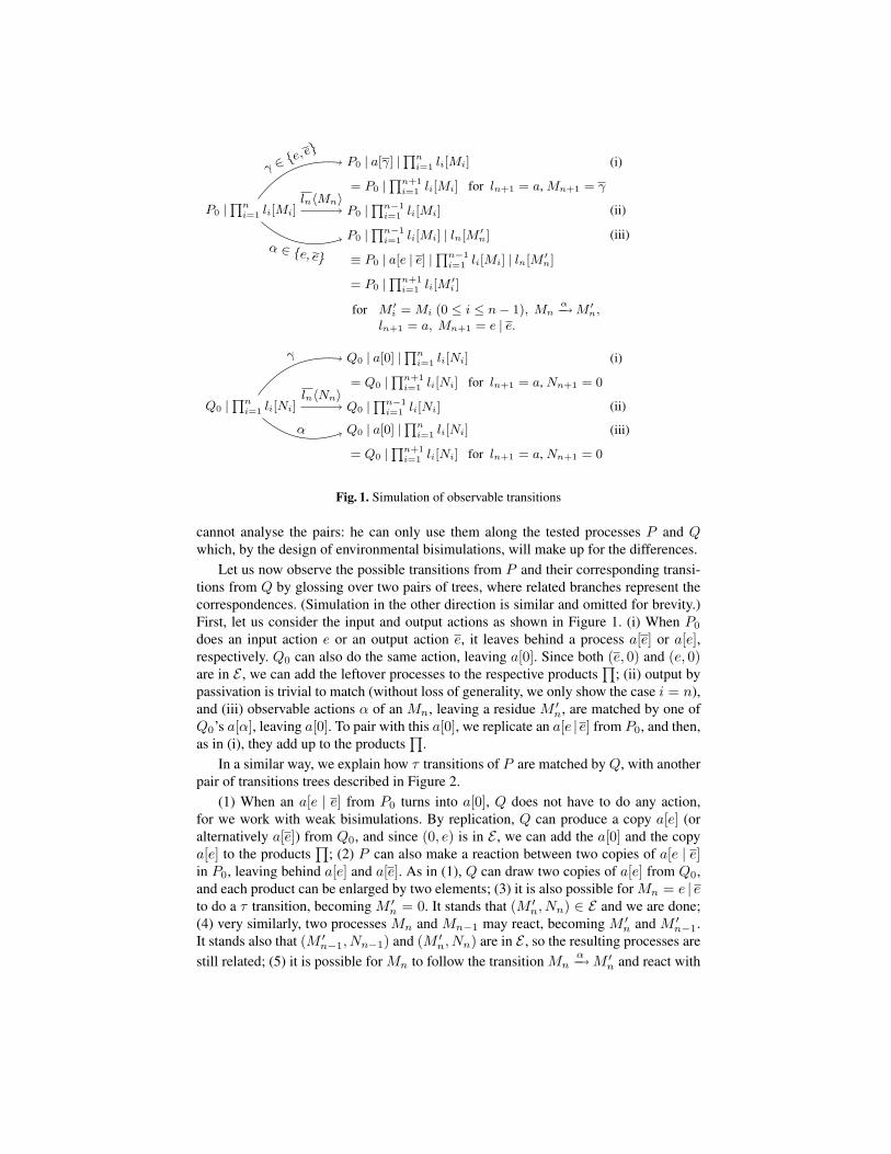
Let us now observe the possible transitions from P and their corresponding transi-tions from Q by glossing over two pairs of trees, where related branches represent thecorrespondences. (Simulation in the other direction is similar and omitted for brevity.)First, let us consider the input and output actions as shown in Figure 1. (i) When P0

does an input action e or an output action e, it leaves behind a process a[e] or a[e],respectively. Q0 can also do the same action, leaving a[0]. Since both (e, 0) and (e, 0)are in E , we can add the leftover processes to the respective products

∏; (ii) output by

passivation is trivial to match (without loss of generality, we only show the case i = n),and (iii) observable actions α of an Mn, leaving a residue M ′

n, are matched by one ofQ0’s a[α], leaving a[0]. To pair with this a[0], we replicate an a[e |e] from P0, and then,as in (i), they add up to the products

∏.

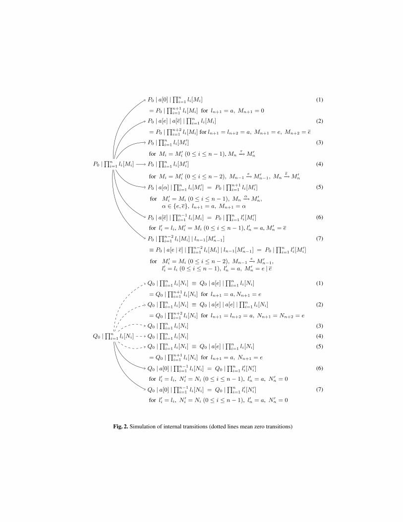
In a similar way, we explain how τ transitions of P are matched by Q, with anotherpair of transitions trees described in Figure 2.

(1) When an a[e | e] from P0 turns into a[0], Q does not have to do any action,for we work with weak bisimulations. By replication, Q can produce a copy a[e] (oralternatively a[e]) from Q0, and since (0, e) is in E , we can add the a[0] and the copya[e] to the products

∏; (2) P can also make a reaction between two copies of a[e | e]

in P0, leaving behind a[e] and a[e]. As in (1), Q can draw two copies of a[e] from Q0,and each product can be enlarged by two elements; (3) it is also possible for Mn = e | eto do a τ transition, becoming M ′

n = 0. It stands that (M ′n, Nn) ∈ E and we are done;

(4) very similarly, two processes Mn and Mn−1 may react, becoming M ′n and M ′

n−1.It stands also that (M ′

n−1, Nn−1) and (M ′n, Nn) are in E , so the resulting processes are

still related; (5) it is possible for Mn to follow the transition Mnα−→M ′

n and react with

P0 | a[0] |Qn

i=1 li[Mi] (1)

= P0 |Qn+1

i=1 li[Mi] for ln+1 = a, Mn+1 = 0

P0 | a[e] | a[e] |Qn

i=1 li[Mi] (2)

= P0 |Qn+2

i=1 li[Mi] for ln+1 = ln+2 = a, Mn+1 = e, Mn+2 = e

P0 |Qn

i=1 li[M′i ] (3)

for Mi = M ′i (0 ≤ i ≤ n− 1), Mn

τ−→M ′n

P0 |Qn

i=1 li[Mi] P0 |Qn

i=1 li[M′i ] (4)

for Mi = M ′i (0 ≤ i ≤ n− 2), Mn−1

e−→M ′n−1, Mn

e−→M ′n

P0 | a[α] |Qn

i=1 li[M′i ] = P0 |

Qn+1i=1 li[M

′i ] (5)

for M ′i = Mi (0 ≤ i ≤ n− 1), Mn

α−→M ′n,

α ∈ {e, e}, ln+1 = a, Mn+1 = α

P0 | a[e] |Qn−1

i=1 li[Mi] = P0 |Qn

i=1 l′i[M′i ] (6)

for l′i = li, M ′i = Mi (0 ≤ i ≤ n− 1), l′n = a, M ′

n = e

P0 |Qn−2

i=1 li[Mi] | ln−1[M′n−1] (7)

≡ P0 | a[e | e] |Qn−2

i=1 li[Mi] | ln−1[M′n−1] = P0 |

Qni=1 l′i[M

′i ]

for M ′i = Mi (0 ≤ i ≤ n− 2), Mn−1

e−→M ′n−1,

l′i = li (0 ≤ i ≤ n− 1), l′n = a, M ′n = e | e

Q0 |Qn

i=1 li[Ni] ≡ Q0 | a[e] |Qn

i=1 li[Ni] (1)

= Q0 |Qn+1

i=1 li[Ni] for ln+1 = a, Nn+1 = e

Q0 |Qn

i=1 li[Ni] ≡ Q0 | a[e] | a[e] |Qn

i=1 li[Ni] (2)

= Q0 |Qn+2

i=1 li[Ni] for ln+1 = ln+2 = a, Nn+1 = Nn+2 = e

Q0 |Qn

i=1 li[Ni] (3)

Q0 |Qn

i=1 li[Ni] Q0 |Qn

i=1 li[Ni] (4)

Q0 |Qn

i=1 li[Ni] ≡ Q0 | a[e] |Qn

i=1 li[Ni] (5)

= Q0 |Qn+1

i=1 li[Ni] for ln+1 = a, Nn+1 = e

Q0 | a[0] |Qn−1

i=1 li[Ni] = Q0 |Qn

i=1 l′i[N′i ] (6)

for l′i = li, N ′i = Ni (0 ≤ i ≤ n− 1), l′n = a, N ′

n = 0

Q0 | a[0] |Qn−1

i=1 li[Ni] = Q0 |Qn

i=1 l′i[N′i ] (7)

for l′i = li, N ′i = Ni (0 ≤ i ≤ n− 1), l′n = a, N ′

n = 0

Fig. 2. Simulation of internal transitions (dotted lines mean zero transitions)

a copy from P0 which leaves behind a[α] (since α has been consumed to conclude thereaction). Again, it stands that M ′

n and Nn are related by E , and that we can draw ana[e] from Q0 to pair it with the residue M ′

n in the products∏

; (6) also, a copy a[e | e]from P0 may passivate an li[Mi], provided li = e, and leave a residue a[e]. Q can dothe same passivation using Q0’s a[e], and leave a[0]. As it happens that (e, 0) is in E ,the residues can be added to the products too; (7) finally, the process ln[Mn], if ln = e,may be passivated by Mn−1, reducing the size of P ’s product. Q can passivate ln[Nn]too, using a copy a[e] from P0, which becomes a[0] after the reaction. Q’s product toois shorter, but we need to add the a[0] to it. To do so, we draw a copy a[e | e] from P0,and since (e | e, 0) is in E , a[e | e] and a[0] are merged into their respective product.

This ends the sketch of the proof thatX is an environmental bisimulation, and there-fore that !a[e | e] and !a[e] | a[e] are behaviourally equivalent.

1.3 Overview of the paper

The rest of this paper is structured as follows. In Section 2 we describe the higher-orderπ-calculus with passivation. In Section 3 we formalize our environmental bisimulations.In Section 4 we give some examples of bisimilar processes. In Section 5, we bring upsome future work to conclude our paper.

2 Higher-order π-calculus with passivation

We introduce a slight variation of the higher-order π-calculus with passivation [7]—HOπP for short—through its syntax and a labelled transitions system.

2.1 Syntax

The syntax of our HOπP processes P , Q is given by the following grammar, verysimilar to that of Lenglet et al. [7] (the higher-order π-calculus extended with locatedprocesses and their passivation):

P,Q ::= 0 | a(X).P | a〈M〉.P | (P | P ) | a[P ] | νa.P | !P | run(M)M,N ::= X | ‘P

X ranges over the set of variables, and a over the set of names which can be used forboth locations and channels. a[P ] denotes the process P running in location a. To definea general up-to context technique (Definition 2, see also Section 5), we distinguish termsM , N from processes P , Q and adopt explicit syntax for processes as terms ‘P and theirexecution run(M).

2.2 Labelled transitions system

We define n , fn , bn and fv to be the functions that return respectively the set of names,free names, bound names and free variables of a process or an action. We abbreviate a(possibly empty) sequence x0, x1, . . . , xn as x for any meta-variable x. The transitionsemantics of HOπP is given by the following labelled transition system, which is basedon that of the higher-order π-calculus (omitting symmetric rules PAR-R and REACT-R):

a(X).Pa(M)−−−→ P{M/X}

HO-INa〈M〉.P a〈M〉−−−→ P

HO-OUT

P1α−→ P ′

1 bn(α) ∩ fn(P2) = ∅P1 | P2

α−→ P ′1 | P2

PAR-L!P | P α−→ P ′

!Pα−→ P ′ REP

P1(νeb).a〈M〉−−−−−−→ P ′

1 P2a(M)−−−→ P ′

2 {eb} ∩ fn(P2) = ∅P1 | P2

τ−→ νeb.(P ′1 | P ′

2)REACT-L

Pα−→ P ′ a 6∈ n(α)

νa.Pα−→ νa.P ′ GUARD

P(νeb).a〈M〉−−−−−−→ P ′ c 6= a c ∈ fn(M) \ {eb}

νc.Pν(eb,c).a〈M〉−−−−−−−→ P ′

EXTR

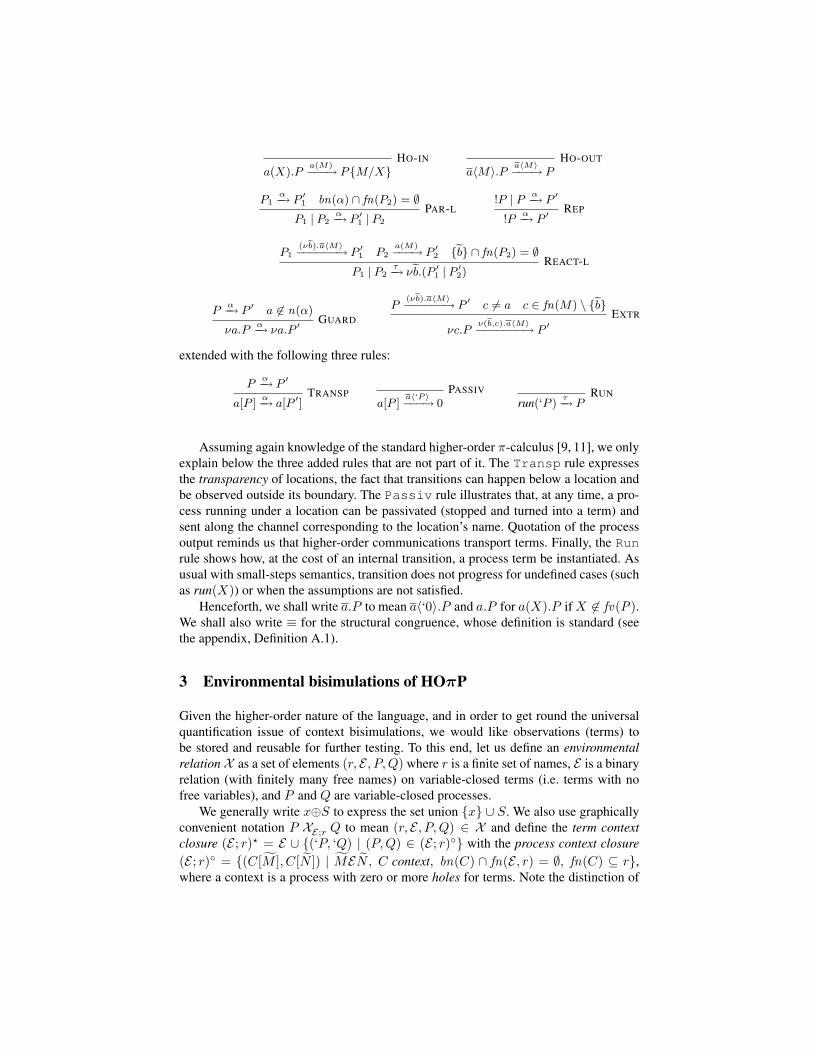
extended with the following three rules:

Pα−→ P ′

a[P ]α−→ a[P ′]

TRANSPa[P ]

a〈‘P 〉−−−→ 0PASSIV

run(‘P )τ−→ P

RUN

Assuming again knowledge of the standard higher-order π-calculus [9, 11], we onlyexplain below the three added rules that are not part of it. The Transp rule expressesthe transparency of locations, the fact that transitions can happen below a location andbe observed outside its boundary. The Passiv rule illustrates that, at any time, a pro-cess running under a location can be passivated (stopped and turned into a term) andsent along the channel corresponding to the location’s name. Quotation of the processoutput reminds us that higher-order communications transport terms. Finally, the Runrule shows how, at the cost of an internal transition, a process term be instantiated. Asusual with small-steps semantics, transition does not progress for undefined cases (suchas run(X)) or when the assumptions are not satisfied.

Henceforth, we shall write a.P to mean a〈‘0〉.P and a.P for a(X).P if X 6∈ fv(P).We shall also write ≡ for the structural congruence, whose definition is standard (seethe appendix, Definition A.1).

3 Environmental bisimulations of HOπP

Given the higher-order nature of the language, and in order to get round the universalquantification issue of context bisimulations, we would like observations (terms) tobe stored and reusable for further testing. To this end, let us define an environmentalrelation X as a set of elements (r, E , P, Q) where r is a finite set of names, E is a binaryrelation (with finitely many free names) on variable-closed terms (i.e. terms with nofree variables), and P and Q are variable-closed processes.

We generally write x⊕S to express the set union {x} ∪ S. We also use graphicallyconvenient notation P XE;r Q to mean (r, E , P, Q) ∈ X and define the term contextclosure (E ; r)? = E ∪ {(‘P, ‘Q) | (P,Q) ∈ (E ; r)◦} with the process context closure(E ; r)◦ = {(C[M ], C[N ]) | MEN , C context, bn(C) ∩ fn(E , r) = ∅, fn(C) ⊆ r},where a context is a process with zero or more holes for terms. Note the distinction of

terms ‘P , ‘Q from processes P , Q. We point out that (∅; r)? is the identity on termswith free names in r, that (E ; r)? includes E by definition, and that the context closureoperations are monotonic on E (and r). Therefore, for any E and r, the set (E ; r)?

includes the identity (∅; r)? too. Also, we use the notations S.1 and S.2 to denote thefirst and second projections of a relation (i.e. set of pairs) S. Finally, we define weaktransitions =⇒ as the reflexive, transitive closure of τ−→, and α=⇒ as =⇒ α−→ =⇒ for α 6= τ(and define τ=⇒ as =⇒).

We can now define environmental bisimulations formally:

Definition 1. An environmental relationX is an environmental bisimulation if P XE;r Qimplies:

1. if Pτ−→ P ′, then ∃Q′. Q =⇒Q′ and P ′ XE;r Q′,

2. if Pa(M)−−−→ P ′ with a ∈ r, and if (M,N) ∈ (E ; r)?, then ∃Q′. Q

a(N)===⇒ Q′ and

P ′ XE;r Q′,

3. if Pνeb.a〈M〉−−−−−→ P ′ with a ∈ r and b 6∈ fn(r, E .1), then ∃Q′, N. Q

νec.a〈N〉=====⇒ Q′ with

c 6∈ fn(r, E .2) and P ′ X(M,N)⊕E;r Q′,4. for any (‘P1, ‘Q1) ∈ E and a ∈ r, we have P | a[P1] XE;r Q | a[Q1],5. for any n 6∈ fn(E , P, Q), we have P XE;n⊕r Q, and6. the converse of 1, 2 and 3 on Q’s transitions.

Modulo the symmetry resulting from clause 6, clause 1 is usual; clause 2 enforcesbisimilarity to be preserved by any input that can be built from the knowledge, hencethe use of the context closure; clause 3 enlarges the knowledge of the observer with theleaked out terms. Clause 4 allows the observer to spawn (and immediately run) termsconcurrently to the tested processes, while clause 5 shows that he can also create freshnames at will.

A few points related to the handling of free names are worth mentioning: as the setof free names in E is finite, clause 5 can always be applied; therefore, the attacker canadd arbitrary fresh names to the set r of known names so as to use them in terms M andN in clause 2. Fresh b and c in clause 3 also exist thanks to the finiteness of free namesin E and r.

We define environmental bisimilarity ∼ as the union of all environmental bisimula-tions, and it holds that it is itself an environmental bisimulation (all the conditions aboveare monotone on X ). Therefore, P ∼E;r Q if and only if P XE;r Q for some environ-mental bisimulation X . We do particularly care about the situation where E = ∅ andr = fn(P,Q). It corresponds to the equivalence of two processes when the observerknows all of their free names (and thus can do all observations), but has not yet learntany output pair.

For improving the practicality of our bisimulation proof method, let us devise an up-to context technique [11, p. 86]: for an environmental relation X , we write P X ?

E;r Q

if P ≡ νc.(P0 | P1), Q ≡ νd.(Q0 | Q1), P0 XE′;r′ Q0, (P1, Q1) ∈ (E ′; r′)◦, E ⊆(E ′; r′)?, r ⊆ r′, and {c} ∩ fn(r, E .1) = {d} ∩ fn(r, E .2) = ∅. As a matter of fact,this is actually an up-to context and up-to environment and up-to restriction and up-tostructural congruence technique, but because of the clumsiness of this appellation we

will restrain ourselves to “up-to context” to preserve clarity. To roughly explain theconvenience behind this notation and its (long) name: (1) “up-to context” states that wecan take any (P1, Q1) from the (process) context closure (E ′; r′)◦ of the environment E ′(with free names in r′) and execute them in parallel with processes P0 and Q0 relatedby XE′;r′ ; similarly, we allow environments E with terms that are not in E ′ itself butare in the (term) context closure (E ′; r′)?; (2) “up-to environment” states that, whenproving the bisimulation clauses, we please ourselves with environments E ′ that arelarger than the E requested by Definition 1; (3) “up-to restriction” states that we alsocontent ourselves with tested processes P , Q with extra restrictions νc and νd (i.e. lessobservable names); (4) finally, “up-to structural congruence” states that we identify allprocesses that are structurally congruent to νc.(P0 | P1) and νd.(Q0 |Q1).

Using this notation, we define environmental bisimulations up-to context as follows:

Definition 2. An environmental relation X is an environmental bisimulation up-to con-text if P XE;r Q implies:

1. if Pτ−→ P ′, then ∃Q′. Q =⇒Q′ and P ′ X ?

E;r Q′,

2. if Pa(M)−−−→ P ′ with a ∈ r, and if (M,N) ∈ (E ; r)?, then ∃Q′. Q

a(N)===⇒ Q′ and

P ′ X ?E;r Q′,

3. if Pνeb.a〈M〉−−−−−→ P ′ with a ∈ r and b 6∈ fn(r, E .1), then ∃Q′, N. Q

νec.a〈N〉=====⇒ Q′ with

c 6∈ fn(r, E .2) and P ′ X ?(M,N)⊕E;r Q′,

4. for any (‘P1, ‘Q1) ∈ E and a ∈ r, we have P | a[P1] X ?E;r Q | a[Q1],

5. for any n 6∈ fn(E , P, Q), we have P XE;n⊕r Q, and6. the converse of 1, 2 and 3 on Q’s transitions.

The conditions on each clause (except 5, which is unchanged for the sake of tech-nical convenience) are weaker than that of the standard environmental bisimulations,as we require in the positive instances bisimilarity modulo a context, not just bisim-ilarity itself. It is important to remark that, unlike in [12] but as in [13], we do notneed a specific context to avoid stating a tautology in clause 4; indeed, we spawn terms(‘P1, ‘Q1) ∈ E immediately as processes P1 and Q1, while the context closure can onlyuse the terms under an explicit run operator.

We prove the soundness (under some condition; see Remark 1) of environmen-tal bisimulations as follows. Full proofs are found in the appendix, Section B but arenonetheless sketched below.

Lemma 1 (Input lemma). If (P1, Q1) ∈ (E ; r)◦ and P1a(M)−−−→ P ′

1 then ∀N.∃Q′1.

Q1a(N)−−−→Q′

1 and (P ′1, Q

′1) ∈ ((M,N)⊕E ; r)◦.

Lemma 2 (Output lemma). If (P1, Q1) ∈ (E ; r)◦, {b}∩fn(E , r) = ∅ and P1νeb.a〈M〉−−−−−→

P ′1 then ∃Q′

1, N. Q1νeb.a〈N〉−−−−−→Q′

1, (P ′1, Q

′1) ∈ (E ; b⊕r)◦ and (M,N) ∈ (E ; b⊕r)?.

Definition 3 (Run-erasure). We write P ≤ Q if P can be obtained by (possibly repeat-edly) replacing zero or more subprocesses run(‘R) of Q with R, and write P Y−

E;r Qfor P ≤ Y?

≤E≥;r ≥ Q.

Definition 4 (Simple environment). A process is called simple if none of its subpro-cesses has the form νa.P or a(X).P with X ∈ fv(P ). An environment is called simpleif all the processes in it are simple. An environmental relation is called simple if all ofits environments are simple (note that the tested processes may still be non-simple).

Lemma 3 (Reaction lemma). For any simple environmental bisimulation up-to con-text Y , if P Y−

E;r Q and Pτ−→ P ′, then there is a Q′ such that Q

τ=⇒Q′ and P ′ Y−E;r Q′.

Proof sketch. Lemma 1 (resp. 2) is proven by straightforward induction on the transition

derivation of P1a(M)−−−→P ′

1 (resp. P1νeb.a〈M〉−−−−−→P ′

1). Lemma 3 is proven last, as it uses theother two lemmas (for the internal communication case).

Lemma 4 (Soundness of up-to context). Simple bisimilarity up-to context is includedin bisimilarity.

Proof sketch. By checking that {(r, E , P, Q) | P Y−E;r Q} is included in ∼, where Y

is the simple environmental bisimilarity up-to context. In particular, we use Lemma 1for clause 2, Lemma 2 for clause 3, and Lemma 3 for clause 1 of the environmentalbisimulation.

Our definitions of reduction-closed barbed equivalence ≈ and congruence ≈c arestandard and omitted for brevity; see the appendix, Definition B.2 and B.3

Theorem 1 (Barbed equivalence from environmental bisimulation).If P Y−

∅;fn(P,Q) Q for a simple environmental bisimulation up-to contextY , then P ≈ Q.

Proof sketch. By verifying that each clause of the definition of ≈ is implied by mem-bership of Y−, using Lemma 4 for the parallel composition clause.

Corollary 1 (Barbed congruence from environmental bisimulation).If a〈‘P 〉 Y−

∅;a⊕fn(P,Q) a〈‘Q〉 for a simple environmental bisimulation up-to context Y ,then P ≈c Q.

We recall that, in context bisimulations, showing the equivalence of a〈‘P 〉 and a〈‘Q〉almost amounts to testing the equivalence of P and Q in every context. However, withenvironmental bisimulations, only the location context in clause 4 of the bisimulationhas to be considered.

Remark 1. The extra condition “simple” is needed because of a technical difficulty inthe proof of Lemma 3: when an input process a(X).P is spawned under location bin parallel with an output context νc.a〈M〉.Q (with c ∈ fn(M)), they can make thetransition b[a(X).P | νc.a〈M〉.Q] τ−→ b[νc.(P{M/X} | Q)], where the restriction op-erator νc appears inside the location b (and therefore can be passivated together withthe processes); however, our spawning clause only gives us b[a(X).P ] | νc.a〈M〉.Q τ−→νc.(b[P{M/X}] | Q) and does not cover the above case. Further investigation is re-quired to overcome this difficulty (although we have not yet found a concrete coun-terexample of soundness, we conjecture some modification to the bisimulation clauseswould be necessary). Note that, even if the environments are simple, the tested processesdo not always have to be simple, as in Example 4 and 5. Moreover, thanks to up-to con-text, even the output terms (including passivated processes) can be non-simple.

4 Examples

Here, we give some examples of HOπP processes whose behavioural equivalence isproven with the help of our environmental bisimulations. In each example, we prove theequivalence by exhibiting a relation X containing the two processes we consider, andby showing that it is indeed a bisimulation up-to context (and environment, restrictionand structural congruence). We write P | . . . | P for a finite, possibly null, product ofthe process P .

Example 1. e | !a[e] | !a[0] ≈ !a[e] | !a[0]. (This example comes from [7].)

Proof. Take X = {(r, ∅, e | P, P ) | r ⊇ {a, e}} ∪ {(r, ∅, P, P ) | r ⊇ {a, e}} whereP = !a[e] | !a[0]. It is immediate to verify that whenever P

α−→ P ′, we have P ′ ≡ P ,and therefore that transition e | P α−→ e | P ′ ≡ e | P can be matched by P

α−→ P ′ ≡ P

and conversely. Also, for e | P e−→ P , we have that Pe−→ !a[e] | a[0] | !a[0] ≡ P and we

are done since (r, ∅, P, P ) ∈ X . Moreover, the set r must contain the free names of P ,and to satisfy clause 5 about adding fresh names, bigger r’s must be allowed too. Thepassivations of a[e] and a[0] can be matched by syntactically equal actions with the pairsof output terms (‘e, ‘e) and (‘0, ‘0) included in the identity, which in turn is included inthe context closure (∅; r)?. Finally clause 4 of the bisimulation is vacuously satisfiedbecause the environment is empty. We therefore have e | !a[e] | !a[0] ≈ !a[e] | !a[0] fromthe soundness of environmental bisimulation up-to context.

Example 2. !a | !e ≈ !a[e].

Proof sketch. Take X = {(r, E , P, Q) | r ⊇ {a, e, l1, . . . , ln} | E = {(‘0, ‘e)}, n ≥ 0,P = !a | !e |

∏ni=1 li[0], Q = !a[e] |

∏ni=1 li[e] | a[0] | . . . | a[0]}. See the appendix,

Example C.1 for the rest of the proof.

Example 3. !a[e] | !b[e] ≈ !a[b[e |e]]. This example shows the equivalence proof of morecomplicated processes with nested locations.

Proof sketch. Take:

X = {(r, E , P, Q) | r ⊇ {a, e, b, l1, . . . , ln},P0 = !a[e] | !b[e], Q0 = !a[b[e | e]],P = P0 |

∏ni=1 li[Pi] | b[0] | . . . | b[0],

Q = Q0 |∏n

i=1 li[Qi],(‘P , ‘Q) ∈ E , n ≥ 0},

E = {(‘x, ‘y) | x ∈ {0, e, e}, y ≡∈ {0, e, e, (e | e), b[0], b[e], b[e], b[e | e]}} .

See the appendix, Example C.2 for the rest of the proof.

Example 4. c(X).run(X) ≈ νf.(f [c(X).run(X)] | !f(Y ).f [run(Y )]). The latter pro-cess models a system where a process c(X).run(X) runs in location f , and executesany process P it has received. In parallel is a process f(Y ).f [run(Y )] which can passi-vate f [P ] and respawn the process P under the same location f . Informally, this modelsa system which can restart a computer and resume its computation after a failure.

Proof. Take X = X1 ∪ X2 where:

X1 = {(r, ∅, c(X).run(X), νf.(f [c(X).run(X)] | !f(Y ).f [run(Y )])) | r ⊇ {c}},X2 = {(r, ∅, P, Q) | r ⊇ c⊕fn(R), S = run(‘run(. . . ‘run(‘R) . . . )),

P ∈ {run(‘R), R}, Q = νf .(f [S] | !f(Y ).[run(Y )])}.

As usual, we require that r contains at least the free name c of the tested processes. Alloutputs belong to (∅; r)? since they come from a process R drawn from (∅; r)?, andtherefore, we content ourselves with an empty environment ∅. Also, by the emptinessof the environment, clause 4 of environmental bisimulations is vacuously satisfied.

Verification of transitions of elements of X1, i.e. inputs of some ‘R (with (‘R, ‘R) ∈(∅; r)?) from c, is immediate and leads to checking elements of X2. For elements ofX2, we observe that P = run(‘R) can do one τ transition to become R, while Qcan do an internal transition passivating the process run(‘R) running in f and placeit inside f [run(‘ )], again and again. Q can also do τ transitions that consume all therun(‘ )’s until it becomes R. Whenever P (resp. Q) makes an observable transition, Q(resp. P ) can consume the run(‘ )’s and weakly do the same action as they exhibitthe same process. We observe that all transitions preserve membership in X2 (thusin X ), and therefore we have that X is an environmental bisimulation up-to context,which proves the behavioural equivalence of the original processes c(X).run(X) andc(X).νf.(f [c(X).run(X)] | !f(Y ).f [run(Y )]).

Example 5. c(X).run(X) ≈ c(X).νa.(a〈X〉 | !νf.(f [a(X).run(X)] | f(Y ).a〈Y 〉)).This example is a variation of Example 4 modelling a system where computation isresumed on another computer after a failure.

Proof. Take X = X1 ∪ X2 ∪ X3 where:

X1 = {(r, ∅, c(X).run(X), c(X).νa.(a〈X〉 | F )) | r ⊇ {c}},X2 = {(r, ∅, P1, νa.(F |R1 |R2 | a〈‘P2〉)) |

r ⊇ {c}⊕fn(P ), P1, P2 ∈ {run(‘P ), P}, R1 = a〈N1〉 | . . . | a〈Nn〉,R2 = νl1.(l1[Q1] | l1(Y ).a〈Y 〉) | . . . | νlm.(lm[Qm] | lm(Y ).a〈Y 〉),N1, . . . , Nn, ‘Q1, . . . , ‘Qm = ‘run(‘run(. . . ‘run(‘a(X).run(X)) . . . )), n ≥ 0},

X3 = {(r, ∅, P1, νa.(F |R1 |R2 | νl.(l[P2] | l(Y ).a〈Y 〉))) |r ⊇ {c}⊕fn(P ), P1, P2 ∈ {run(‘P ), P}, R1 = a〈N1〉 | . . . | a〈Nn〉,R2 = νl1.(l1[Q1] | l1(Y ).a〈Y 〉) | . . . | νlm.(lm[Qm] | lm(Y ).a〈Y 〉),N1, . . . , Nn, ‘Q1, . . . , ‘Qm = ‘run(‘run(. . . ‘run(‘a(X).run(X)) . . . )), n ≥ 0},

F = !νf.(f [a(X).run(X)] | f(Y ).a〈Y 〉).

The set of names r and the environment share the same fate as those of Example 4for identical reasons. For ease, we write lhs and rhs to conveniently denote each of thetested processes.

Verification of the bisimulation clauses of X1 is immediate and leads to a member(r, ∅, run(‘P ), νa.(a〈‘P 〉 | F )) of X2 for some ‘P with (‘P, ‘P ) ∈ (∅; r)?. For X2, lhscan do an internal action (consuming its outer run(‘ )) that rhs does not have to followsince we work with weak bisimulations, and the results is still inX2; conversely, internalactions of rhs do not have to be matched. Some of those transitions that rhs can do are

reactions between replications from F . All those transitions creates elements of eitherR1 or R2 that can do nothing but internal actions and can be ignored further in the proofthanks to the weakness of our bisimulations.

Whenever lhs does an observable action α, that is, when P1 = Pα−→P ′, rhs must do

a reaction between a〈‘P2〉 and F , giving νl.(l[P2] | l(Y ).a〈Y 〉) α=⇒νl.(l[P ′] | l(Y ).a〈Y 〉)which satisfies X3’s definition. Moreover, all transitions of P1 or P2 in X3 can bematched by the other, hence preserving the membership in X3. Finally, a subprocessνl.(l[P2] | l(Y ).a〈Y 〉) of rhs of X3 can do a τ transition to a〈‘P2〉 and the residuesbelong back to X2.

This concludes the proof of behavioural equivalence of the original processes c(X).run(X)and c(X).νa.(a〈X〉.!νf.(f [a(X).run(X)] | f(Y ).f [run(Y )])).

5 Discussion and future work

In the original higher-order π-calculus with passivation described by Lenglet et al. [7],terms are identified with processes: its syntax is just P ::= 0 | X | a(X).P | a〈P 〉.P |(P |P ) | a[P ] | νa.P | !P . We conjecture that it is also possible to develop sound envi-ronmental bisimulations (and up-to context, etc.) for this version of HOπP, as we [12]did for the standard higher-order π-calculus. However we chose not to cover directly theoriginal higher-order π-calculus with passivation, for two reasons: (1) the proof methodof [12] which relies on guarded processes and a factorisation trick using the spawn-ing clause of the bisimulation is inadequate in the presence of locations; (2) there is avery strong constraint in clause 4 of up-to context in [12, Definition E.1 (Appendix)](the context has no hole for terms from E). By distinguishing processes from terms, notonly is our up-to context method much more general, but our proofs are also direct andtechnically simple. Although one might argue that the presence of the run operator is aburden, by using Definition 3, one could devise an “up-to run” technique and abstractrun(. . . ‘run(‘P )) as P , making equivalence proofs easier to write and understand.

As described in Remark 1, removing the limitation on the environments is left forfuture work. We also plan to apply environmental bisimulations to (a substantial subsetof) the Kell calculus so that we can provide a practical alternative to context bisimula-tions in a more expressive higher-order distributed process calculus. In the Kell calculus,locations are not transparent: one discriminates messages on the grounds of their ori-gins (i.e. from a location above, below, or from the same level). For example, considerthe (simplified) Kell processes P = a〈M〉.!b[a] and Q = a〈N〉.!b[a] where M = aand N = 0. They seem bisimilar assuming environmental bisimulations naively likethose in this paper: intuitively, both P and Q can output (respectively M and N ) tochannel a, and their continuations are identical; passivation of spawned l[M ] and l[N ]for known location l would be immediately matched; finally, the output to channel aunder l, turning P ’s spawned l[M ] into l[0], could be matched by an output to a under bby Q’s replicated b[a]. However, M and N behave differently when observed from thesame level (or below), for example as in l[M | a(Y ).ok] and l[N | a(Y ).ok] even underthe presence of !b[a]. More concretely, the context [·]1 | a(X).c[X | a(Y ).ok] distin-guishes P and Q, showing the unsoundness of such naive definition. This suggests that,to define sound environmental bisimulations in Kell-like calculi with non-transparent

locations, we should require a stronger condition such as bisimilarity of M and N inthe output clause. Developments on this idea are in progress.

References

1. L. Cardelli and A. D. Gordon. Mobile ambients. In Foundations of Software Science andComputation Structures, volume 1378 of Lecture Notes in Computer Science, pages 140–155. Springer, 1998.

2. M. Hennessy and J. Riely. Resource access control in systems of mobile agents. Informationand Computation, 173:82–120, 1998.

3. Hewlett-Packard. Live migration across data centers and disaster tolerant virtual-ization architecture with HP storageworks cluster extension and Microsoft Hyper-V.http://h20195.www2.hp.com/V2/GetPDF.aspx/4AA2-6905ENW.pdf.

4. T. Hildebrandt, J. C. Godskesen, and M. Bundgaard. Bisimulation congruences for Homer:a calculus of higher-order mobile embedded resources. Technical Report TR-2004-52, ITUniversity of Copenhagen, 2004.

5. K. Honda and N. Yoshida. On reduction-based process semantics. Theoretical ComputerScience, 151(2):437–486, 1995.

6. D. J. Howe. Proving congruence of bisimulation in functional programming languages, 1996.7. S. Lenglet, A. Schmitt, and J.-B. Stefani. Normal bisimulations in calculi with passivation.

In Foundations of Software Science and Computational Structures, volume 5504 of LectureNotes in Computer Science, pages 257–271. Springer, 2009.

8. R. Milner. Communicating and Mobile Systems: the Pi-Calculus. Cambridge UniversityPress, 1999.

9. D. Sangiorgi. Expressing Mobility in Process Algebras: First-Order and Higher-OrderParadigms. PhD thesis, University of Edinburgh, 1992.

10. D. Sangiorgi. Bisimulation for higher-order process calculi. Information and Computation,131:141–178, 1996.

11. D. Sangiorgi. The π-calculus: a Theory of Mobile Processes. Cambridge University Press,2001.

12. D. Sangiorgi, N. Kobayashi, and E. Sumii. Environmental bisimulations for higher-orderlanguages. In Proceedings of the Twenty-Second Annual IEEE Symposium on Logic in Com-puter Science, pages 293–302, 2007.

13. N. Sato and E. Sumii. The higher-order, call-by-value applied pi-calculus. In Asian Sympo-sium on Programming Languages and Systems, volume 5904 of Lecture Notes in ComputerScience, pages 311–326. Springer, 2009.

14. D. Schmidt and P. Dhawan. Live migration with Xen virtualization software.http://www.dell.com/downloads/global/power/ps2q06-20050322-Schmidt-OE.pdf.

15. A. Schmitt and J.-B. Stefani. The Kell calculus: A family of higher-order distributed processcalculi. In Global Computing, volume 3267 of Lecture Notes in Computer Science, pages146–178. Springer, 2004.

16. E. Sumii and B. C. Pierce. A bisimulation for dynamic sealing. Theoretical ComputerScience, 375(1-3):169–192, 2007. Extended abstract appeared in Proceedings of 31st AnnualACM SIGPLAN-SIGACT Symposium on Principles of Programming Languages, pp. 161–172, 2004.

17. E. Sumii and B. C. Pierce. A bisimulation for type abstraction and recursion. Journal ofthe ACM, 54:1–43, 2007. Extended abstract appeared in Proceedings of 32nd Annual ACMSIGPLAN-SIGACT Symposium on Principles of Programming Languages, pp. 63–74, 2005.

Appendix for “Sound Bisimulations for Higher-OrderDistributed Process Calculus”

Adrien Pierard and Eijiro Sumii

Tohoku University{adrien,sumii}@kb.ecei.tohoku.ac.jp

A Higher-order π-calculus with passivation

1 Syntax

The syntax of HOπP processes P , Q is given by the following grammar:

P,Q ::= 0 | a(X).P | a〈M〉.P | (P | P ) | a[P ] | νa.P | !P | run(M)M,N, V, W ::= X | ‘P

We define the functions that returns the free names and free variables respectively as:

fn(0) = ∅ fv(0) = ∅fn(a(X).P ) = {a} ∪ fn(P ) fv(a(X).P ) = fv(P ) \ {X}fn(a〈M〉.P ) = {a} ∪ fn(M) ∪ fn(P ) fv(a〈M〉.P ) = fv(M) ∪ fv(P )fn(P1 | P2) = fn(P1) ∪ fn(P2) fv(P1 | P2) = fv(P1) ∪ fv(P2)fn(a[P ]) = {a} ∪ fn(P ) fv(a[P ]) = fv(P )fn(νa.P ) = fn(P ) \ {a} fv(νa.P ) = fv(P )fn(!P ) = fn(P ) fv(!P ) = fv(P )fn(run(M)) = fn(M) fv(run(M)) = fv(M)fn(X) = ∅ fv(X) = {X}fn(‘P ) = fn(P ) fv(‘P ) = fv(P )

We conveniently write fn(X, Y, . . . , Z) (resp. fv(X, Y, . . . , Z)) to denote⋃

S∈{X,Y,...,Z} fn(S)(resp.

⋃S∈{X,Y,...,Z} fv(S)).

2 Labelled transitions system

The transitions semantics of HOπP is given by the following labelled transitions system:

a(X).Pa(M)−−−→ P{M/X}

HO-IN

a〈M〉.P a〈M〉−−−→ PHO-OUT

P1α−→ P ′

1 bn(α) ∩ fn(P2) = ∅P1 | P2

α−→ P ′1 | P2

PAR-LP2

α−→ P ′2 bn(α) ∩ fn(P1) = ∅

P1 | P2α−→ P1 | P ′

2

PAR-R

P1(νeb).a〈M〉−−−−−−→ P ′

1 P2a(M)−−−→ P ′

2 {b} ∩ fn(P2) = ∅P1 | P2

τ−→ νb.(P ′1 | P ′

2)REACT-L

P1a(M)−−−→ P ′

1 P2(νeb).a〈M〉−−−−−−→ P ′

2 {b} ∩ fn(P1) = ∅P1 | P2

τ−→ νb.(P ′1 | P ′

2)REACT-R

Pα−→ P ′ a 6∈ n(α)

νa.Pα−→ νa.P ′ GUARD

!P | P α−→ P ′

!P α−→ P ′ REP

P(νeb).a〈M〉−−−−−−→ P ′ c 6= a c ∈ fn(M) \ {b}

νc.Pν(eb,c).a〈M〉−−−−−−−→ P ′

EXTR

Pα−→ P ′

a[P ] α−→ a[P ′]TRANSP

a[P ]a〈‘P 〉−−−→ 0

PASSIV

run(‘P ) τ−→ PRUN

with the following functions on labels

n(α) =

∅ if α = τ

{a} ∪ fn(V ) if α = a(V ){a, b} ∪ fn(V ) if α = νb.a〈V 〉

bn(α) =

{∅ if α = τ or α = a(V ){b} if α = νb.a〈V 〉

and the notation x to denote the sequence x1, x2, . . . xn.

Definition A.1. Structural congruence ≡ is the smallest relation on processes suchthat:

Q ≡ P

P ≡ QS-SYM

P ≡ PS-REFL

P ≡ R R ≡ Q

P ≡ QS-TRANS

P ≡ P | 0S-EMPTY

P1 | (P2 | P3) ≡ (P1 | P2) | P3

S-ASSOCP1 | P2 ≡ P2 | P1

S-COMMUT

νa.0 ≡ 0S-NULL

νa.νb.P ≡ νb.νa.PS-SWAP

a 6∈ fn(P1)P1 | (νa.P2) ≡ νa.(P1 | P2)

S-SCOPE

P ≡ Q

νa.P ≡ νa.QS-GUARD

P ≡ Q

a(X).P ≡ a(X).QS-IN

P1 ≡ Q1 P2 ≡ Q2

a〈‘P1〉.P2 ≡ a〈‘Q1〉.Q2

S-OUT

!P ≡ !P | PS-REP

P ≡ Q

!P ≡ !QS-BANG

P1 ≡ Q1 P2 ≡ Q2

P1 | P2 ≡ Q1 |Q2

S-COMP

P ≡ Q

a[P ] ≡ a[Q]S-LOC

P ≡ Q

run(‘P ) ≡ run(‘Q)S-RUN

Definition A.2. Structural congruence on labels ≡ is defined by:

τ ≡ τL-TAU

M ≡ N

a(M) ≡ a(N)L-IN

M ≡ N

νc.a〈M〉 ≡ νc.a〈N〉L-OUT

Lemma A.3. [Reduction preserves structural congruence]If P ≡ Q then

(a) for all α, P ′, if Pα−→ P ′ then either

i. there are c, a, M such that if α ≡ νc.a〈M〉 or α ≡ τ , then there are β, Q′

such that Qβ−→Q′, α ≡ β and P ′ ≡ Q′, or

ii. there are a, M such that if α ≡ a(M), then for all β such that α ≡ β, there is

Q′ such that Qβ−→Q′ and P ′ ≡ Q′, and

(b) for all α, Q′, if Qα−→Q′ then either

i. there are c, a, M such that if α ≡ νc.a〈M〉 or α ≡ τ , then there are β, P ′

such that Pβ−→ P ′, α ≡ β and P ′ ≡ Q′, or

ii. there are a, M such that if α ≡ a(M), then for all β such that α ≡ β, there is

P ′ such that Pβ−→ P ′ and P ′ ≡ Q′.

Proof. By induction on the derivations of P ≡ Q.

B Environmental bisimulations of HOπP

1 Notations

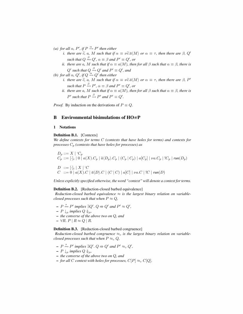
Definition B.1. [Contexts]We define contexts for terms C (contexts that have holes for terms) and contexts forprocesses Cp (contexts that have holes for processes) as

Dp ::= X | ‘Cp

Cp ::= [·]i | 0 | a(X).Cp | a〈Dp〉.Cp | (Cp | Cp) | a[Cp] | νa.Cp | !Cp | run(Dp)

D ::= [·]i | X | ‘CC ::= 0 | a(X).C | a〈D〉.C | (C | C) | a[C] | νa.C | !C | run(D)

Unless explicitly specified otherwise, the word “context” will denote a context for terms.

Definition B.2. [Reduction-closed barbed equivalence]Reduction-closed barbed equivalence ≈ is the largest binary relation on variable-

closed processes such that when P ≈ Q,

– Pτ−→ P ′ implies ∃Q′. Q =⇒Q′ and P ′ ≈ Q′,

– P ↓µ implies Q ⇓µ,– the converse of the above two on Q, and– ∀R. P |R ≈ Q |R.

Definition B.3. [Reduction-closed barbed congruence]Reduction-closed barbed congruence ≈c is the largest binary relation on variable-

closed processes such that when P ≈c Q,

– Pτ−→ P ′ implies ∃Q′. Q =⇒Q′ and P ′ ≈c Q′,

– P ↓µ implies Q ⇓µ,– the converse of the above two on Q, and– for all C context with holes for processes, C[P ] ≈c C[Q].

2 Soundness of environmental bisimulations

Lemma B.4. [Originally Lemma 1 “Input lemma”]

If (P1, Q1) ∈ (E ; r)◦ and P1a(M)−−−→ P ′

1 then ∀N.∃Q′1. Q1

a(N)−−−→ Q′1 ∧ (P ′

1, Q′1) ∈

((M,N)⊕E ; r)◦.

Proof. By induction on the transition derivation P1a(M)−−−→ P ′

1. There are six cases tocheck.

1. Case IN: C = a(X).C1

We have that P1 = a(X).C1[M ]a(M)−−−→C1[M ]{M/X} and that Q1 = a(X).C1[N ]

a(N)−−−→C1[N ]{N/X}. We are done since we replace term X by terms M and N , henceC1[M ]{M/X}((M,N)⊕E ; r)◦C1[N ]{N/X}.

2. Case PAR-L: C = C1 | C2

We have that P1 = C1[M ] |C2[M ]a(M)−−−→P ′ |C2[M ], i.e. C1[M ]

a(M)−−−→P ′. By the

induction hypothesis C1[N ]a(N)−−−→ Q′ and P ′((M,N)⊕E ; r)◦Q′, from which we

derive (P ′ | C2[M ])((M,N)⊕E ; r)◦(Q′ | C2[N ]) as well as C1[N ] | C2[N ]a(N)−−−→

Q′ | C2[N ].3. Case PAR-R: C = C1 | C2

Similar.4. Case TRANSP: C = l[C1]

We have that P1 = l[C1[M ]]a(M)−−−→ l[P ′], that is C1[M ]

a(M)−−−→P ′. By the induction

hypothesis, we have that C1[N ]a(N)−−−→ Q′ and P ′((M,N)⊕E ; r)◦Q′, from which

we derive l[P ′]((M,N)⊕E ; r)◦l[Q′] as well as l[C1[N ]]a(N)−−−→ l[Q′].

5. Case GUARD: C = νb.C1

We have that P1 = νb.C1[M ]a(M)−−−→ νb.P ′, i.e. C1[M ]

a(M)−−−→P ′, b 6∈ n(a,M) and

C1[M ](E ; b⊕r)◦C1[N ]. By the induction hypothesis, we have C1[N ]a(N)−−−→Q′ and

P ′((M,N)⊕E ; b⊕r)◦Q′, hence νb.P ′((M,N)⊕E ; r)◦νb.Q′. Finally, νb.C1[N ]a(N)−−−→

Q′.6. Case REP: C = !C1

We have that P1 = !C1[M ]a(M)−−−→P ′, i.e. !C1[M ]|C1[M ]

a(M)−−−→P ′. By the induction

hypothesis, we have that !C1[N ] |C1[N ]a(N)−−−→Q′ and P ′((M,N)⊕E ; r)◦Q′. Thus

!C1[N ]a(N)−−−→Q′ and still P ′((M,N)⊕E ; r)◦Q′.

Lemma B.5. [Originally Lemma 2, “Output lemma”]

If P1 (E ; r)◦Q1, {b}∩ fn(E , r) = ∅ and P1νeb.a〈M〉−−−−−→P ′

1 then ∃Q′1, N. Q1

νeb.a〈N〉−−−−−→Q′1,

P ′1(E ; b⊕r)◦Q′

1 and M (E ; b⊕r)? N .

Proof. By induction on the transition derivation P1νeb.a〈M〉−−−−−→ P ′

1. There are eight casesto check.

1. Case OUTPUT: C = a〈‘C1〉.C2

We have that P1 = a〈‘C1[M ]〉.C2[M ]a〈‘C1[fM ]〉−−−−−−→ C2[M ] and that

Q1 = a〈‘C1[N ]〉.C2[N ]a〈‘C1[ eN ]〉−−−−−−→C2[N ]. It is immediate to confirm that ‘C1[M ](E ; r)?

‘C1[N ] and C2[M ] (E ; r)◦ C2[N ] hold.2. Case PAR-L: C = C1 | C2

We have that P1 = C1[M ] |C2[M ]νeb.a〈M〉−−−−−→P ′ |C2[M ], i.e. C1[M ]

νeb.a〈M〉−−−−−→P ′ and

{b} ∩ fn(C2[M ]) = ∅. By the induction hypothesis, we have that C1[N ]νeb.a〈N〉−−−−−→

Q′ and P ′(E ; (b⊕r))◦Q′ and M (E ; (b⊕r))? N . Since b 6∈ fn(C2[M ])–i.e. b 6∈

fn(C2)–and b 6∈ E , we have that C1[N ] | C2[N ]νeb.a〈N〉−−−−−→ Q′ | C2[N ], and

(P ′ | C2[M ])(E ; (b⊕r))◦(Q′ | C2[N ]).3. Case PAR-R: C = C1 | C2

Similar.4. Case TRANSP: C = l[C1]

We have that P1 = l[C1[M ]]νeb.a〈M〉−−−−−→ l[P ′], i.e. C1[M ]

νeb.a〈M〉−−−−−→P ′. By the induc-

tion hypothesis, we have C1[N ]νeb.a〈N〉−−−−−→Q′, P ′(E ; (b⊕r))◦Q′ and M (E ; (b⊕r))?

N . From this we derive l[C1[N ]]νeb.a〈N〉−−−−−→ l[Q′] and l[P ′](E ; (b⊕r))◦l[Q′] and we

are done.5. Case PASSIV: C = l[C1]

We have that P1 = l[C1[M ]]l〈‘C1[fM ]〉−−−−−−→0. Immediately, we have Q1 = l[C1[N ]]

l〈‘C1[ eN ]〉−−−−−−→0 with ‘C1[M ] (E ; r)? ‘C1[N ] and 0 (E ; r)◦ 0.

6. Case GUARD: C = νc.C1

By the definition of process context closure, it holds that C1[M ](E ; c⊕r)◦C1[N ].

We also have that P1 = νc.C1[M ]νeb.a〈M〉−−−−−→ νc.P ′, i.e. C1[M ]

νeb.a〈M〉−−−−−→P ′ and c 6∈

{b, a}∪fn(M). By the induction hypothesis, we have C1[N ]νeb.a〈N〉−−−−−→Q′, C0[M ] =

M(E ; (b⊕c⊕r))?N = C0[N ] and P ′(E ; (b⊕c⊕r))◦Q′, hence νc.P ′(E ; (b⊕r))◦νc.Q′.Moreover, since c 6∈ fn(M), we have c 6∈ fn(C0), and since c 6∈ fn(E) it also holds

that c 6∈ fn(C0[N ]), hence νc.C1[N ]νeb.a〈N〉−−−−−→ νc.Q′ and M (E ; (b⊕r))? N .

7. Case REP: C = !C1

We have that P1 = !C1[M ]νeb.a〈M〉−−−−−→ P ′, i.e. !C1[M ] | C1[M ]

νeb.a〈M〉−−−−−→ P ′. By the

induction hypothesis, we have !C1[N ] | C1[N ]νeb.a〈N〉−−−−−→Q′, M (E ; (b⊕r))? N and

P ′(E ; (b⊕r))◦Q′, hence !C1[N ]νeb.a〈N〉−−−−−→Q′ and we are done.

8. Case EXTR: C = νc.C1

We have that P1 = νc.C1[M ]νeb,c.a〈M〉−−−−−−→ P ′, i.e. C1[M ]

νeb.a〈M〉−−−−−→ P ′ withC1[M ](E ; c⊕r)◦C1[N ] a 6= c, c ∈ fn(M) \ {b}. By the induction hypothesis, we

have C1[N ]νeb.a〈N〉−−−−−→Q′ and M (E ; (b⊕c⊕r))? N and P ′(E ; (b⊕c⊕r))◦Q′. Since

c ∈ fn(M) \ {b}, we have c ∈ fn(C0[M ]) \ {b}. Since c 6∈ fn(r, E), by the defi-

nition of context closure necessarily c ∈ fn(C0) \ {b}, hence c ∈ fn(C0[N ]) \ {b}

i.e. c ∈ fn(N) \ {b}. We are then done since νc.C1[N ]νeb,c.a〈N〉−−−−−−→Q′.

Lemma B.6. [Input and output preserve environmental bisimulation up-to context]LetY be an environmental bisimulation up-to context andX = {(r, E , P, Q) | P Y?

E;r Q}.Then, for all P XE;r Q,

1. if Pa(V )−−−→ P ′ with a in r, then for all (V,W ) ∈ (E ; r)? there is a Q′ such that

Qa(W )===⇒Q′ and P ′ XE;r Q′,

2. if Pνec1.a〈V 〉−−−−−−→ P ′ with a in r and c1 6∈ fn(E .1, r) , then there is a Q′ such that

Qν ed1.a〈W 〉======⇒Q′ with d1 6∈ fn(E .2, r) and P ′ X(V,W )⊕E;r Q′, and

3. the converse of the above two hold for Q’s transitions too.

Proof. Suppose P Y?E;r Q, therefore for some P0, P1, Q0, Q1, E ′, r′, c, d, we have

P ≡ νc.(P0 |P1), Q ≡ νd.(Q0 |Q1), r ⊆ r′, {c}∩ fn(r, E .1) = {d}∩ fn(r, E .2) = ∅,E ⊆ (E ′; r′)?, P0 YE′;r′ Q0 and P1 (E ′; r′)◦ Q1.

We are going to analyse all the possible input/output transitions.

1. Case: InputThere are two cases for this transition:(a) Subcase: P0

a(V )−−−→ P ′0 {c} ∩ n(a(V )) = ∅

By P0 YE′;r′ Q0, we have Q0a(W )===⇒ Q′

0 and P ′0 Y?

E′;r′ Q′0. It then holds that

νc.(P0 | P1)a(V )−−−→ ≡ νc, c1.(P ′

00 | P ′01 | P1) ≡ P ′. Also, since V (E ; r)? W ,

we have that fn(W ) ⊆ fn(r, E .2), and since d ∩ fn(r, E .2) = ∅, we have that

νd.(Q0 |Q1)a(W )===⇒ ≡ νd, d1.(Q′

00 |Q′01 |Q1) ≡ Q′. P ′ Y?

E;r Q′ follows, henceP ′ XE;r Q′.

(b) Subcase: P1a(V )−−−→ P ′

1 {c} ∩ n(a(V )) = ∅By Lemma B.4, we have that Q1

a(W )−−−→Q′1 and P ′

1 ((V,W )⊕E ′; r′)◦Q′1. Since

(E ; r)? ⊆ (E ′; r′)?, we actually have P ′1 (E ′; r′)◦ Q′

1. Then, we have νc.(P0 |P1)

a(V )−−−→ νc.(P0 |P ′1) ≡ P ′ and νd.(Q0 |Q1)

a(W )−−−→ νd.(Q0 |Q′1) ≡ Q′ since

d 6∈ fn(r, E .2). Therefore, P ′ Y?E;r Q′, that is, P ′ XE;r Q′.

2. Case: OutputThere are two cases for this transition:(a) Subcase: P0

νei.a〈V 〉−−−−−→ P ′0

We have {i} = {c1}\{c}, that is {i} 6∈ fn(r, E .1). In order to apply clause 3 ofthe bisimulation, we may need to substitute a fresh variable not in fn(r′, E ′) fori in P ′

0 and V below, and we will assume that it has been done to release someburden from the proof. Let P ′ = νcr.(P ′

0 |P1) and i, co = c1. By P0 YE′;r′ Q0,

we have Q0νej.a〈W 〉=====⇒ Q′

0, j 6∈ fn(r′, E ′.2) and P ′0 Y?

(V,W )⊕E′;r′ Q′0. Also, we

have that νd.(Q0 | Q1)νej, edo.a〈W 〉=======⇒ νdr.(Q′

0 | Q1) with {do} ⊆ {d} and do ∈fn(W ) \ {j}, and we then define d1 = j, do. By P ′

0 Y?(V,W )⊕E′;r′ Q′

0, we have

– P ′0 = νc2.(P00 | P01), Q′

0 = νd2.(Q00 |Q01),– c2 6∈ fn(E ′.1, r′), d2 6∈ fn(E ′.2, r′),– P00 YE′′;r′′ Q00, P01 (E ′′; r′′)◦ Q01,– (V,W )⊕E ′ ⊆ (E ′′; r′′)?, r′ ⊆ r′′.

Since P1 (E ′; r′)◦ Q1, we have (P1 | P01) (E ′′; r′′)◦ (Q1 | Q01). Since E ⊆(E ′; r′)?, we have (V,W )⊕E ⊆ ((V,W )⊕E ′; r′)? ⊆ (E ′′; r′′)?. Finally, cr, c2 6∈fn(E .1, r) and dr, d2 6∈ fn(E .2, r), P ′ ≡ νcr, c2.(P00 | P01 | P1) and Q′ ≡νdr, d2.(Q00 | Q01 | Q1), from where we conclude that P Y?

(V,W )⊕E;r Q, thatis, after undoing the potential substitution, P X(V,W )⊕E;r Q.

(b) Subcase: P1νei.a〈V 〉−−−−−→ P ′

1

We have {i} ⊆ {c1}, that is, i 6∈ fn(r, E .1) and νc.(P0 |P ′1)

νec1.a〈V 〉−−−−−−→νcr.(P0 |P ′

1) = P ′ with {cr} = {c} \ {c1}. In order to apply Lemma B.5, we may needto substitute a fresh variable not in fn(r′, E ′) for i in P ′

1, Q′1, V and W below,

and we will assume that it has been done to release some burden from the proof.

By Lemma B.5, we have that Q1νei.a〈W 〉−−−−−→ Q′

1 and V (E ′; i⊕r′)? W as wellas P ′

1 (E ′; i⊕r′)◦ Q′1. Then, since we can assume {i} ∩ fn(Q0) = ∅, we have

Q0 |Q1νei.a〈W 〉−−−−−→Q0 |Q′

1, and therefore νd.(Q0 |Q1)νei, edo−−−→νdr.(Q0 |Q′

1) ≡ Q′,with d1 = i, do and {d1} ∩ fn(r, E .2) = ∅. So far, we have

– P0 YE′;r′ Q0, that is P0 YE′;ei⊕r′Q0 since {i} ∩ fn(E ′, r′) = ∅,

– P ′1 (E ′; i⊕r′)◦ Q′

1,– E ⊆ (E ′; r′)? ⊆ (E ′; i⊕r′)?,– r ⊆ r′ ⊆ i⊕r′.– {cr} ∩ fn(r, E .1) = {dr} ∩ fn(r, E .2) = ∅

hence P ′ Y?E;r Q′ and therefore, after undoing the potential substitution, P ′ XE;r Q′.

3. Case: The converse of the above two cases on Q’s transitions.Similar to clauses 1 and 2.

Definition B.7. [run-erasure and run-expansion]For all processes A, B, we write A < B and B > A if there are Cp and R such thatA = Cp[R] and B = Cp[run‘(R)]. We write P0 ≤ Pn if P0 < · · · < Pn for somen ≥ 0. We naturally write A ≥ B whenever B ≤ A. We naturally extend ≤ and ≥’sdefinitions to terms and labels.

We use the metavariables P+ and P− along with P when we mean that P ≤ P+

and that P− ≤ P . (The notations (·)+ and (·)− therefore do not represent operators.)Similarly, we use the metavariables M+ and M− to represent run-expansions and run-erasures of term M .

Lemma B.8. [Input, output and reduction preserve < and > ]Let X = {(r, E , P, Q) | P < Q, E ⊆ < }. If P XE;r Q, then

– if Pτ−→P ′ then there is a Q′ such that P ′ XE;r Q′ and either Q

τ−→Q′ or Qrun−−→ τ−→Q′,

– if Pa(M)−−−→P ′ then for all (M,N) ∈ (E ; r)? there is a Q′ such that P ′ XE;r Q′ and

either Qa(N)−−−→Q′ or Q

run−−→ a(N)−−−→Q′,

– if Pνec.a〈M〉−−−−−→P ′ then there are Q′, M < N such that P ′ X(M,N)⊕,E;r Q′ and either

Qνec.a〈N〉−−−−−→Q′ or Q

run−−→ νec.a〈N〉−−−−−→Q′, and– the converse on Q’s transitions.

Similarly for > .

Proof. By induction on the derivation transition of Cp[R] (or Cp[run(‘R)]). We onlyshow the HO-IN derivation case of the input preservation, the others being straightfor-ward or similar.

– Case P ’s input:There are two subcases: the context inputs, or some Ri.

• P = Cp[R]a(M)−−−→C ′

p[R,M ] by an input from the context, and thus for (M,N) =

(C ′′p [A], C ′′

p [run‘A]) ∈ < , Q = Cp[run‘R]a(N)−−−→C ′

p[run‘R, run‘C ′′p [run‘A]] τ−→

C ′p[run‘R, C ′′

p [run‘A]] = C ′′′p [run‘R, run‘A]. We are done as C ′

p[R,M ] =C ′

p[R, C ′′p [‘A]] = C ′′′

p [R, A] < C ′′′p [run‘R, run‘A].

• P = Cp[R, R]a(M)−−−→ Cp[R, R′] by an input from R, and thus for (M,N) =

(C ′′p [A], C ′′

p [run‘A]) ∈ < , we have Q = Cp[run‘R, run‘R] τ−→Cp[run‘R, R]a(N)−−−→

Cp[run‘R, R′′]. Since (R′, R′′) = (C ′′′p [A], C ′′′

p [run‘A]), we have R′ < R′′ andtherefore Cp[R, R′] < Cp[run‘R, R′′] and we are done.

– Case Q’s input:There is only one subcase, as no Ri can input for they are all guarded.

• Q = Cp[run‘R]a(N)−−−→C ′

p[run‘R,N ] by an input from the context, and thus for

(M,N) = (C ′′p [A], C ′′

p [run‘A]) ∈ < , P = Cp[‘R]a(M)−−−→ C ′

p[R, C ′′p [A]] =

C ′′′p [R, A]. We are done as C ′

p[run‘R,N ] = C ′p[run‘R, C ′′

p [run‘A]]= C ′′′

p [run‘R, run‘A] > C ′′′p [R, A].

Corollary B.9. [Input, output and reduction preserve ≤ and ≥ ]For all r, for any closed P , Q, the sets X1 = {(r, E , P0, Pm) | E ⊆ ≤, P0 ≤ Pm},

and X2 = {(r, E , P0, Pm) | E ⊆ ≥, P0 ≥ Pm} are both preserved by input, outputand reduction.

Proof. By induction on the number n of < (in ≤) (resp. on the number of > (in ≥)).We explicitly treat only the set X1, the set X2 being treated similarly.

– Case n = 0Trivial.

– Case n > 0We have P0

α−→ P ′0, hence by Lemma B.8 either

• P1β−→ P ′

1 with α < β and P ′0 < P ′

1. By P1 ≤ Pn (which has n − 1 “<”),applying the induction hypothesis we have Pn

γ=⇒P ′

n with β ≤ γ, hence α ≤ γ,and P ′

0 ≤ P ′n, or

• P1τ−→ P ′′

1β−→ P ′

1 with α < β and P ′0 < P ′

1. By P1 ≤ Pn (which has n − 1“<”), applying the induction hypothesis with P1

τ−→P ′′1 , we have Pn

τ=⇒P ′′n and

P ′′1 ≤ P ′′

n . Then we apply again the induction hypothesis to P ′′1 ≤ P ′′

n and

P ′′1

β−→ P ′1, and we obtain P ′′

nγ=⇒ P ′′

n and P ′1 ≤ P ′

n with β ≤ γ, hence P ′0 ≤ P ′

n

and α ≤ γ.

Definition B.10. [run-transition]We write P

run−−→P ′ when Pτ−→P ′ is derived using the rule RUN. Then, we write P0

runn

==⇒Pn to mean that P0

run−−→ . . .run−−→ Pn.

Definition B.11. [Minimal transition of run-expanded processes]

Suppose that A ≤ B, Aα−→ A′, B

runn

==⇒ β−→B′ with α ≤ β and that A′ ≤ B′. We say

that Brunn

==⇒ β−→B′ is minimal with respect to Aα−→A′ if and only if for all B

runm

==⇒ γ−→B′′

with A′ ≤ B′′ and α ≤ γ, we have n ≤ m.

Lemma B.12. [Minimality and run-transition]

Suppose that Brun−−→ B′′ runn−1

====⇒ β−→B′ with n > 0 is minimal with respect to Aα−→ A′.

We have that B′′ runn−1

====⇒ β−→B′ too is minimal with respect to Aα−→A′.

Proof. By reductio ad absurdum. Suppose that B′′ runn−1

====⇒ β−→B′ is not minimal withrespect to A

α−→A′. There must be a minimal transition B′′ runm

==⇒ γ−→B′′′ with A′ ≤ B′′′,α ≤ γ, and m < n − 1. Then we have a derivation B

run−−→ B′′ runm

==⇒ γ−→B′′′ of length

m+1 < n with A′ ≤ B′′′, which contradicts the assumption that B run−−→B′′ runn−1

====⇒ β−→B′

is minimal.

Lemma B.13. [Minimality and contexts]

For all Qrunn

==⇒ β−→Q′ minimal with respect to Pα−→ P ′,

– for all R1 ≥ R2, Q |R1runn

==⇒ β−→Q′ |R1 is minimal with respect to P |R2α−→P ′ |R2,

– for l, l[Q] runn

==⇒ β−→l[Q′] is minimal with respect to l[P ] α−→ l[P ′], and– if Q = Q0 | Q1, Q′ = Q′

0 | Q′1, and P = P0 | P1 with P0 ≤ Q0, P1 ≤ Q1,

then for all l and m, l[Q0] |m[Q1]runn

==⇒ β−→l[Q′0] |m[Q′

1] is minimal with respect tol[P0] |m[P1]

α−→ l[P ′0] |m[P ′

1].

– for all c, νc.Qrunn

==⇒ β′−→νc′.Q′′ is minimal with respect to Pα′−→ P ′′.

Proof. Immediate, as none of the above operations can reduce the number of run’s thathave to be deleted, and as they all preserve membership to ≤.

Definition B.14. [run-erased context closure]We define the run-erased context closure (E ; r)− of environment E with names r as≤ (E ; r)? ≥ , that is {(M,N) | M ≤ A, N ≤ B, (A,B) ∈ (E ; r)?}. Notice that

(E ; r)− may erase run’s inside elements related by E too.We also write P Y−

E;r Q if P ≤ Y?≤E≥;r ≥ Q (which implies Y? ⊆ Y−). In other

words P Y−E;r Q if P ≡ νc.(P0|P1), Q ≡ νd.(Q0|Q1), P0 ≤ YE′;r′ ≥ Q0, (‘P1, ‘Q1) ∈

(E ; r)−, E ⊆ (E ′; r′)−, r ⊆ r′, and {c} ∩ fn(E .1, r) = {d} ∩ fn(E .2, r) = ∅.

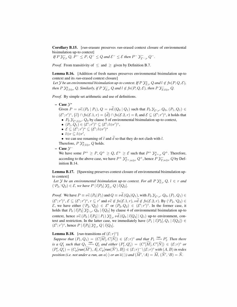
Corollary B.15. [run-erasure preserves run-erased context closure of environmentalbisimulation up-to context]If P Y−

E;r Q, P− ≤ P , Q− ≤ Q and E− ≤ E then P− Y−E−;r Q−.

Proof. From transitivity of ≤ and ≥ given by Definition B.7.

Lemma B.16. [Addition of fresh names preserves environmental bisimulation up-tocontext and its run-erased context closure]LetY be an environmental bisimulation up-to context. If P Y?

E;r Q and l 6∈ fn(P,Q, E),then P Y?

E;l⊕r Q. Similarly, if P Y−E;r Q and l 6∈ fn(P,Q, E), then P Y−

E;l⊕r Q.

Proof. By simple set arithmetic and use of definitions.

– Case Y?

Given P = νc.(P0 | P1), Q = νd.(Q0 | Q1) such that P0 YE′;r′ Q0, (P1, Q1) ∈(E ′; r′)◦, {c} ∩ fn(E .1, r) = {d} ∩ fn(E .2, r) = ∅, and E ⊆ (E ′; r′)?, it holds that• P0 YE′;l⊕r′ Q0 by clause 5 of environmental bisimulation up-to context,• (P1, Q1) ∈ (E ′; r′)◦ ⊆ (E ′; l⊕r′)◦,• E ⊆ (E ′; r′)? ⊆ (E ′; l⊕r′)?

• l⊕r ⊆ l⊕r′,• we can use renaming of c and d so that they do not clash with l.

Therefore, P Y?E;l⊕r Q holds.

– Case Y−

We have some P+ ≥ P , Q+ ≥ Q, E+ ≥ E such that P+ Y?E+;r Q+. Therefore,

according to the above case, we have P+ Y?E+;n⊕r Q+, hence P Y−

E;n⊕r Q by Def-inition B.14.

Lemma B.17. [Spawning preserves context closure of environmental bisimulation up-to context]Let Y be an environmental bisimulation up-to context. For all P Y?

E;r Q, l ∈ r and(‘P2, ‘Q2) ∈ E , we have P | l[P2] Y?

E;r Q | l[Q2].

Proof. We have P ≡ νc.(P0 |P1) and Q ≡ νd.(Q0 |Q1), with P0 YE′;r′ Q0, (P1, Q1) ∈(E ′; r′)◦, E ⊆ (E ′; r′)?, r ⊆ r′ and νc 6∈ fn(E .1, r), νd 6∈ fn(E .2, r). By (‘P2, ‘Q2) ∈E , we have either (‘P2, ‘Q2) ∈ E ′ or (P2, Q2) ∈ (E ′; r′)◦. In the former case, itholds that P0 | l[P2] Y?

E′;r′ Q0 | l[Q2] by clause 4 of environmental bisimulation up-tocontext, hence νc.(P0 | l[P2] | P1) Y?

E;r νd.(Q0 | l[Q2] |Q1) up-to environment, con-text and restriction. In the latter case, we immediately have (P1 | l[P2], Q1 | l[Q2]) ∈(E ′; r′)◦, hence P | l[P2] Y?

E;r Q | l[Q2].

Lemma B.18. [run-transitions of (E ; r)◦]Suppose that (P1, Q1) = (C[M ], C[N ]) ∈ (E ; r)◦ and that P1

run−−→ P ′1. Then there

is a Q′1 such that Q1

run−−→ Q′1 and either (P ′

1, Q′1) = (C ′[M ], C ′[N ]) ∈ (E ; r)◦ or

(P ′1, Q

′1) = (Cp[run(M ′), A], Cp[run(N ′), B]) ∈ (E ; r)−\(E ; r)◦ with (A,B) in redex

position (i.e. not under a run, an a(·) or an a〈·〉) and (M ′, ‘A) = M , (N ′, ‘B) = N .

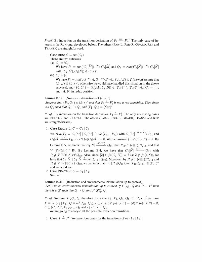
Proof. By induction on the transition derivation of P1run−−→ P1′. The only case of in-

terest is the RUN one, developed below. The others (PAR-L, PAR-R, GUARD, REP andTRANSP) are straightforward.

1. Case RUN: C = run(C1)There are two subcases(a) C1 = ‘C2

We have P1 = run(‘C2[M ]) run−−→ C2[M ] and Q1 = run(‘C2[N ]) run−−→ C2[N ]with (C2[M ], C2[N ]) ∈ (E ; r)◦.

(b) C1 = [·]We have P1 = run(‘A) run−−→A, Q1

run−−→B with (‘A, ‘B) ∈ E (we can assume that(A,B) 6∈ (E ; r)◦, otherwise we could have handled this situation in the abovesubcase), and (P ′

1, Q′1) = (Cp[A], Cp[B]) ∈ (E ; r)− \ (E ; r)◦ with Cp = [·]1,

and (A,B) in redex position.

Lemma B.19. [Non-run τ -transitions of (E ; r)◦]Suppose that (P1, Q1) ∈ (E ; r)◦ and that P1

τ−→ P ′1 is not a run-transition. Then there

is a Q′1 such that Q1

τ−→Q′1 and (P ′

1, Q′1) = (E ; r)◦.

Proof. By induction on the transition derivation P1τ−→ P ′

1. The only interesting casesare REACT-R and REACT-L. The others (PAR-R, PAR-L, GUARD, TRANSP and REPare straightforward.)

1. Case REACT-L: C = C1 | C2

We have P1 = C1[M ] | C2[M ] τ−→ νc.(P11 | P12) with C1[M ]νec.a〈V 〉−−−−−→ P11 and

C2[M ]a(V )−−−→ P12, {c} ∩ fn(C2[M ]) = ∅. We can assume {c} ∩ fn(r, E) = ∅. By

Lemma B.5, we know that C1[N ]νec.〈W 〉−−−−→ Q11, that P11(E ; (c⊕r))◦Q11, and that

V (E ; (c⊕r))? W . By Lemma B.4, we have that C2[N ]a(W )−−−→ Q12 with

P12((V,W )⊕E ; r)◦Q12. Also, since {c} ∩ fn(C2[N ]) = ∅ (as c 6∈ fn(r, E)), wehave that C1[N ] |C2[N ] τ−→ νc.(Q11 |Q12). Moreover, by P11(E ; (c⊕r))◦Q11 andP12((V,W )⊕E ; r)◦Q12, we can infer that (νc.(P11|Q11), νc.(P12|Q12)) ∈ (E ; r)◦

and we are done.2. Case REACT-R: C = C1 | C2

Similar.

Lemma B.20. [Reduction and environmental bisimulation up-to context]Let Y be an environmental bisimulation up-to context. If P Y?

E;r Q and P −→ P ′ thenthere is a Q′ such that Q =⇒Q′ and P ′ Y−

E;r Q′.

Proof. Suppose P Y?E;r Q, therefore for some P0, P1, Q0, Q1, E ′, r′, c, d we have

P ≡ νc.(P0 |P1), Q ≡ νd.(Q0 |Q1), r ⊆ r′, {c}∩ fn(r, E .1) = {d}∩ fn(r, E .2) = ∅,E ⊆ (E ′; r′)?, P0 YE′;r′ Q0 and P1 (E ′; r′)◦ Q1.

We are going to analyse all the possible reduction transitions.

1. Case: Pτ−→ P ′. We have four cases for the transitions of νc.(P0 | P1):

(a) Subcase P0τ−→ P ′

0

By P0 YE′;r′ Q0, we have that Q0 =⇒Q′0 and P ′

0 Y?E′;r′ Q′

0. Therefore, νc.(P0 |P1)

τ−→ νc.(P ′0 | P1) ≡ νc, ci.(P ′

00 | P ′01 | P1) ≡ P ′ since ci does not appear in

P1. Also, νd.(Q0 |Q1) =⇒ νd.(Q′0 |Q1) ≡ νd, di.(Q′

00 |Q′01 |Q1) = Q′ since

di does not appear in Q1. We have cj , dj , P00, Q00, P01, Q01, r′′ and E ′′ suchthat

– P ′0 ≡ νci.(P00 | P01), Q′

0 ≡ νdi.(Q00 |Q01),– ci 6∈ fn(r′, E ′.1), di 6∈ fn(r′, E ′.2),– P00 YE′′;r′′ Q00, P01 (E ′′; r′′)◦ Q01,– E ′ ⊆ (E ′′; r′′)?, r′ ⊆ r′′,

It then holds that E ⊆ (E ′′; r′′)?, r ⊆ r′′ and that c, ci 6∈ fn(r, E .1), d, di 6∈fn(r, E .2). Also, P ′

1 (E ′′; r′′)◦Q′1 hence (P01 |P ′

1) (E ′′; r′′)◦ (Q01 |Q′1). There-

fore P ′ Y?E;r Q′, hence P ′ Y−

E;r Q′.(b) Subcase P1

τ−→ P ′1

Since (P1, Q1) ∈ (E ′; r′)◦, then necessarily P1τ−→ P ′

1 implies that the con-text reduces, and Q1 can do the same derivation. Therefore, by Lemmas B.18and B.19 either (P1, Q1) = (C[M ], C[N ]) ∈ (E ′; r′)◦ and (P ′

1, Q′1)

= (C ′[M ], C ′[N ]) ∈ (E ′; r′)◦ or (P1, Q1) = (C2[‘A, ‘A], C2[‘B, ‘B]) =(Cp[run‘A, run‘A], Cp[run‘B, run‘B]) and (P ′

1, Q′1) = (Cp[run‘A, A], Cp[run‘B, B])

with (‘A, ‘B) ∈ E ′ and (A,B) 6∈ (E ′; r′)◦. In both cases, we have P ′ Y−E;r Q′

and we are done.(c) Subcase P0

νec1.a〈V 〉−−−−−−→ P ′0 P1

a(V )−−−→ P ′1 {c1} ∩ fn(r′, E ′.1) = ∅

By P0 YE′;r′ Q0, we have Q0ν ed1.a〈W 〉======⇒Q′

0 and P ′0 Y?

(V,W )⊕E′;r′ Q′0 with d1 6∈

fn(E ′.2, r′) free in W . Also, since P1a(V )−−−→ P ′

1 we have by Lemma B.4 that

Q1a(W )−−−→ Q′

1 and P ′1 (E ′ ∪ {(V,W )}; r′)◦ Q′

1. Therefore νc.(P0 | P1)τ−→≡

νc, c1.(P ′0 | P ′

1) ≡ P ′ and νd.(Q0 | Q1) =⇒≡ νd, d1.(Q′0 | Q′

1) = Q′. ByP ′

0 Y?(V,W )⊕E′;r′ Q′

0 we have that

– P ′′0 = νc2.(P00 | P01), Q′′

0 = νd2.(Q00 |Q01),– c2 6∈ fn(E ′.1, r′), d2 6∈ fn(E ′.2, r′),– P00 YE′′;r′′ P00, P01 (E ′′; r′′)◦ Q01,– (V,W )⊕E ′ ⊆ (E ′′; r′′)?, r′ ⊆ r′′.

We have νc, c1.(P ′′0 | P ′

1) ≡ νc, c1, c2.(P00 | P01 | P ′1), νd, d1.(Q′′

0 | Q′1) ≡

νd, d1, d2.(Q00 |Q01 |Q′1), E ⊆ (E ′′; r′′)?, r ⊆ r′′, hence (P01 |P ′

1) (E ′′; r′′)◦(Q01 | Q′

1), as well as c, c1, c2 6∈ fn(E .1, r), d, d1, d2 6∈ fn(E .2, r). We thusconclude that P Y−

E;r Q.

(d) Subcase P0a(V )−−−→ P ′

0 P1νes.a〈V 〉−−−−−→ P ′

1

By Lemma B.5, we have for s 6∈ fn(r′, E ′) that Q1νes.a〈W 〉−−−−−→Q′

1 and V (E ′; s⊕r′)?

W , as well as P ′1 (E ′; s⊕r′)◦ Q′

1. Using freshness of s, we have by clause 5 ofthe bisimulation up-to context P0 YE′;es⊕r′ Q0, hence P ′

0 Y?E′;es⊕r′ Q′

0 for some

Q0a(W )===⇒Q′

0, i.e.– P ′

0 = νc1.(P00 | P01), Q′0 = νd1.(Q00 |Q01),

– c1 6∈ fn(E ′.1, s⊕r′), d1 6∈ fn(E ′.2, s⊕r′),– P00 YE′′;r′′ Q00, P01 (E ′′; r′′)◦ Q01,– E ′ ⊆ (E ′′; r′′)?, s⊕r′ ⊆ r′′.

Then, c, s, c1 6∈ fn(E .1, r) and d, s, d1 6∈ fn(E .2, r), νc.(P0 |P1)τ−→ νc, s.(P ′

0 |P ′

1) ≡ νc, s, c1.(P00 | P01 | P ′1) = P ′, and νd.(Q0 |Q1) =⇒ νd, s.(Q′

0 |Q′1) ≡

νd, s, d1.(Q00 | Q01 | Q′1) = Q′. Also r ⊆ r′′ and E ⊆ (E ′′; r′′)?, hence

(P01 | P ′1) (E ′′; r′′)◦ (Q01 |Q′

1). As a result, P ′ Y−E;r Q′.

2. Case: Q reduces.Conversely.

Lemma B.21. [run-expanded output with spawning]Suppose that νc.(P0 | l[P1]) Y?

E;r νd.(Q0 | l[Q1]) for an environmental bisimulation

up-to context Y with l ∈ r and that P1runn

==⇒ νec1.a〈M〉−−−−−−→P ′1 is minimal with respect to

P−1

νec1.a〈M−〉−−−−−−−→ P ′−1 , (so νc.(P0 | l[P1])

runn

==⇒ νec0.a〈M〉−−−−−−→νc′.(P0 | l[P ′1]) is minimal with

respect to νc.(P−0 |l[P−

1 ])νec0.a〈M−〉−−−−−−−→νc′.(P−

0 |l[P ′−1 ])). Then νd.(Q0 | l[Q1])

ν ed0.a〈N〉=====⇒

νd′.(Q′0 | l[Q′

1]), and νcr.P0 Y−(M,N)⊕(‘P ′

1,‘Q′1)⊕E;r νdr.Q

′0 with {c′} = {c} \ fn(M),

{cr} = {c′} \ fn(P ′1), {dr} = {d′} \ fn(Q′

1), and {c′, c0} ∩ fn(E .1, r) = {d′, d0} ∩fn(E .2, r) = {d0} ∩ {d′} = {c0} ∩ {c′} = ∅.

Proof. By induction on n.

– Case n = 0Immediate by Lemma B.6 and the fact that Y? ⊆ Y−.

– Case n > 0By Lemma B.20 and Lemma B.12, we have two possible subcases preserving mini-

mality after the first run-transition of νc.(P0 | l[P1])runn

==⇒ νec0.a〈M〉−−−−−−→νc′.(P0 | l[P ′1]).

• Subcase νc.(P0 | l[P1])run−−→νc.(P0 | l[P ′′

1 ]), νd.(Q0 | l[Q1])=⇒νd′′.(Q′′0 | l[Q′′

1 ])and νc.(P0 | l[P ′′

1 ]) Y?E;r νd′′.(Q′′

0 | l[Q′′1 ]).

As νc.(P0 | l[P ′′1 ]) runn−1

====⇒ νec0.a〈M〉−−−−−−→νc′.(P0 | l[P ′1]) is still minimal with respect

to νc.(P−0 | l[P−

1 ])νec0.a〈M−〉−−−−−−−→ νc′.(P−

0 | l[P ′−1 ]), we can apply the induction

hypothesis and get the desired results.• Subcase νc.(P0 | l[P1])

run−−→νc.(P0 | l[P ′′1 ]), νd.(Q0 | l[Q1])=⇒νd′′.(Q′′

0 | l[Q′′1 ])

and νc.(P0 | l[P ′′1 ]) Y−

E;r νd′′.(Q′′0 | l[Q′′

1 ]), with

(P1, Q1) = (Cp[run(M), run‘A], Cp[run(N), run‘B]) and(P ′′

1 , Q′′1) = (Cp[run(M), A], Cp[run(N), B]) with (A,B) in redex position

(i.e. (‘A, ‘B) ∈ E ′ and (A,B) 6∈ (E ′; r′)◦ for some E ′, r′ such that E ⊆(E ′; r′)?, νc.(P0 | l[P1]) ≡ νx.(PA | PB), νd.(Q0 | l[Q1]) ≡ νy.(QA | QB),PA YE′;r′ QA, (PB , QB) ∈ (r′; E ′)◦, r ⊆ r′, x∩fn(E .1, r) = y∩fn(E .2, r) =∅.

By νc.(P−0 | l[P−

1 ])νec0.a〈M−〉−−−−−−−→ νc′.(P−

0 | l[P ′−1 ]), P1 = Cp[run(M), run‘A],

P ′′1 = Cp[run(M), A] and P−

1 ≤ P ′1, we know that there is a run-erasure

A− ≤ A such that A− is in redex position in P1 and that Aνec1.a〈M〉−−−−−−→ A′

is minimal with respect to A− νec1.a〈M−〉−−−−−−−→ A′−. Using Lemma B.16 (to adda fresh name l), Lemma B.17 and up-to context (to work with P0 and Q0

instead of PA and QA) and environment (to work with E and r instead ofE ′, r′) techniques, we have P0 | l[A] Y?

E;l⊕r Q0 | l[B] and, by Lemma B.13,

P0 | l[A] runn−1

====⇒ νec1.a〈M〉−−−−−−→P0 | l[A′] minimal with respect to P−0 |l[A−]

νec1.a〈M−〉−−−−−−−→

P−0 | l[A′−]. Applying the induction hypothesis, we get Q′′

0 | l[B]ν ed1.a〈N〉=====⇒

νdn.(Q′0 | l[B′]), and P0 Y−

(M,N)⊕(‘A′,‘B′)⊕E;l⊕r νdr1.Q′0 with {dr1} = {dn}\

fn(B), and {dn}∩fn(E .2, l, r) = {d1}∩{dn} = ∅. Therefore, Q′′0 | l[Q′′

1 ]ν ed1.a〈N〉=====⇒

νdn.(Q′0 | l[Q′

1]) for Q′1 = Cp[run(M), B′] since the context Cp cannot bind

names free in E ′, r′, hence in E , B, nor in N . Then νd.(Q0 | l[Q1])ν ed0.a〈N〉=====⇒

νd′.(Q′0 | l[Q′

1]) with {d′} = {dn} ∪ {{d} \ {{d0} \ {d1}}}. And also,P0 Y−

(M,N)⊕(‘A′,‘B′)⊕E;l⊕r νdr1.Q′0 implies P0 Y−

(M,N)⊕(‘P ′1,‘Q′

1)⊕E;r νdr1.Q′0

up-to environment to remove l and build P ′1 and Q′

1, andνcr.P0 Y−

(M,N)⊕(‘P ′1,‘Q′

1)⊕E;r νdr.Q′0 up-to restriction for {cr} = {c′}\fn(P ′

1)

and {dr} = {d′} \ fn(Q′1).

Corollary B.22. [run-expanded output]Suppose that νc.(P0 | P1) Y?

E;r νd.(Q0 |Q1) for an environmental bisimulation up-to

contextY with P0 YE′;r′ Q0, (P1, Q1) ∈ (E ′; r′)◦, {c}∩fn(E .1, r) = {d}∩fn(E .2, r) =

∅, and that νc.(P0 | P1)runn

==⇒ νec0.a〈M〉−−−−−−→νc′.(P ′0 | P ′

1) is minimal with respect to

νc.(P−0 | P−

1 )νec0.a〈M−〉−−−−−−−→νc′.(P ′−

0 | P ′−1 ). Then νd.(Q0 |Q1)

ν ed0.a〈N〉=====⇒νd′.(Q′

0 |Q′1),

and νc′.(P ′0 | P ′

1) Y−(M,N)⊕E;r νd′.(Q′

0 |Q′1) with {d′}∩fn(E .2, r,N) = {d0}∩{d′} =

∅.

Proof. By induction on n.

– Case n = 0Immediate by Lemma B.6 and the fact that Y? ⊆ Y−.

– Case n > 0By Lemma B.20 and Lemma B.12, we have two possible subcases preserving min-

imality after the first run-transition of νc.(P0 | P1)runn

==⇒ νec0.a〈M〉−−−−−−→νc′.(P ′0 | P ′

1).• Subcase P0

run−−→ P ′′0

We have that Q0τ=⇒Q′′

0 and P ′′0 Y?

E′;r′ Q′′0 , and also that P ′′

0runn−1

====⇒ νec1.a〈M〉−−−−−−→P ′0

is minimal with respect to P−0

νec1.a〈M−〉−−−−−−−→ P ′−0 . Thus, we can apply the induc-

tion hypothesis and get Q′′0

ν ed1.a〈N〉=====⇒Q′

0 as well as P ′0 Y−

(M,N)⊕E′;r′ Q′0. There-

fore, Q0 |Q1ν ed1.a〈N〉=====⇒Q′

0 |Q1, hence νd.(Q0 |Q1)ν ed0.a〈N〉=====⇒ νd′.(Q′

0 |Q1).Also, P ′

0 | P1 Y−(M,N)⊕E;r Q′

0 |Q1 up-to environment for using E and r instead

of E ′ and r′ and context for spawning P1 and Q1, and finallyνc′.(P ′

0 | P1) Y−(M,N)⊕E;r νd′′′.(Q′

0 |Q1) up-to restriction for {c′} = {c} \fn(M), {d′′′} ⊇ {d} \ fn(N), {d′} 6∈ fn(E .2, N, r), and d′ = d′′′.

• Subcase P1run−−→ P ′

1

Using Lemma B.16 to add a fresh name l and the fact that (P1, Q1) ∈ (E ′; r′)◦,

we have νc.(P0 | l[P1]) Y?E;l⊕r Q0 | l[Q1]. As νc.(P0 | l[P1])

runn

==⇒ νec0.a〈M〉−−−−−−→

νc.(P0 | l[P ′1]) is minimal with respect to νc.(P−

0 | l[P−1 ])

νec0.a〈M−〉−−−−−−−→

νc′.(P−0 | l[P ′−

1 ]), we can use Lemma B.21 and have νd.(Q0 | l[Q1])ν ed0.a〈N〉=====⇒

νd′.(Q′0 | l[Q′

1]), hence νd.(Q0 | Q1)ν ed0.a〈N〉=====⇒ νd′.(Q′

0 | Q′1) and also

νcr.P0 Y−(M,N)⊕(‘P ′

1,‘Q′1)⊕E;l⊕r νdr.Q

′0 with {cr} = {c′} \ fn(M), {dr} ⊆

{d′} \ fn(N), {d′} ∩ fn(E .2, N, r) = ∅. Therefore,νc′.(P0 | P ′

1) Y−(M,N)⊕E;r νd′.(Q′

0 |Q′1) up-to context, environment and restric-

tion.

Corollary B.23. [Output preserves run-erased environmental bisimulation up-to con-text]

For any environmental bisimulation up-to context Y , if P Y−E;r Q and P

νec.a〈M〉−−−−−→ P ′

with a ∈ r and c 6∈ fn(E .1, r), then there is a Q′ such that Qν ed.a〈N〉=====⇒ Q′ with

d 6∈ fn(E .2, r) and P ′ Y−(M,N)⊕E;r Q′. The converse on Q’s transition holds too.

Proof. By Y−’s definition, we know there are P+, Q+ and E+ such that P+ Y?E+;r Q+.

Since Pνec.a〈M〉−−−−−→ P ′, there is a minimal output transition P+ runn

==⇒ νec.a〈M+〉−−−−−−→P ′+. By

Lemma B.22, we have Q+ νec.a〈N+〉======⇒Q′+ and P ′+ Y−

(M+,N+)⊕E+;r Q′+ which implies

by Corollary B.9 that Q can also weakly do an output transition Qνec.a〈N〉=====⇒ Q′, such

that Q′ ≤ Q′+ and N ≤ N+. By Corollary B.15, as P ′ ≤ P ′+, Q′ ≤ Q′+ and(M,N)⊕E ≤ (M+, N+)⊕E+, we have P ′ Y−

(M,N)⊕E;r Q′ as desired. Visually, thefollowing diagram holds.

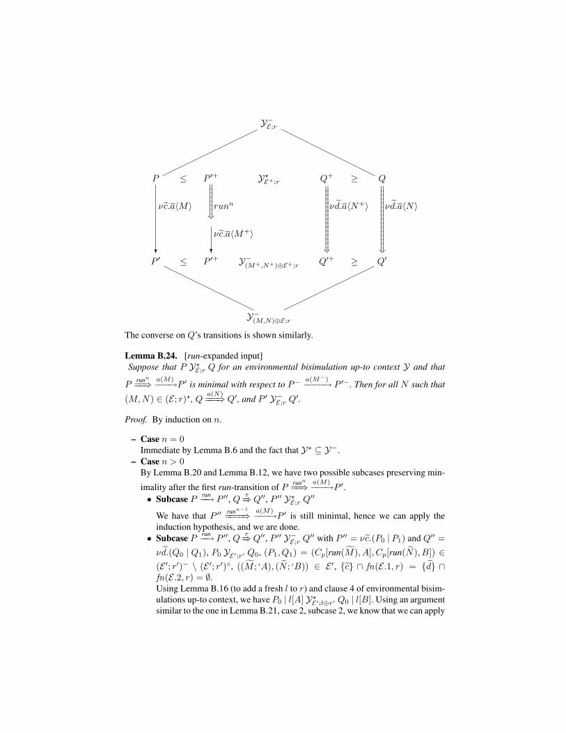
Y−E;r

P ≤ P ′+ Y?E+;r Q+ ≥ Q

runn�wwwwwww

P ′

νc.a〈M〉

?≤ P ′+

νc.a〈M+〉

?Y−

(M+,N+)⊕E+;r Q′+

νd.a〈N+〉

�

wwwwwwwwwwwwwww≥ Q′

νd.a〈N〉

�

wwwwwwwwwwwwwww

Y−(M,N)⊕E;r

The converse on Q’s transitions is shown similarly.

Lemma B.24. [run-expanded input]Suppose that P Y?

E;r Q for an environmental bisimulation up-to context Y and that

Prunn

==⇒ a(M)−−−→P ′ is minimal with respect to P− a(M−)−−−−→ P ′−. Then for all N such that

(M,N) ∈ (E ; r)?, Qa(N)===⇒Q′, and P ′ Y−

E;r Q′.

Proof. By induction on n.

– Case n = 0Immediate by Lemma B.6 and the fact that Y? ⊆ Y−.

– Case n > 0By Lemma B.20 and Lemma B.12, we have two possible subcases preserving min-

imality after the first run-transition of Prunn

==⇒ a(M)−−−→P ′.• Subcase P

run−−→ P ′′, Qτ=⇒Q′′, P ′′ Y?

E;r Q′′

We have that P ′′ runn−1

====⇒ a(M)−−−→P ′ is still minimal, hence we can apply theinduction hypothesis, and we are done.

• Subcase Prun−−→ P ′′, Q

τ=⇒Q′′, P ′′ Y−E;r Q′′ with P ′′ = νc.(P0 | P1) and Q′′ =

νd.(Q0 | Q1), P0 YE′;r′ Q0, (P1, Q1) = (Cp[run(M), A], Cp[run(N), B]) ∈(E ′; r′)− \ (E ′; r′)◦, ((M ; ‘A), (N ; ‘B)) ∈ E ′, {c} ∩ fn(E .1, r) = {d} ∩fn(E .2, r) = ∅.Using Lemma B.16 (to add a fresh l to r) and clause 4 of environmental bisim-ulations up-to context, we have P0 | l[A] Y?

E′;l⊕r′ Q0 | l[B]. Using an argumentsimilar to the one in Lemma B.21, case 2, subcase 2, we know that we can apply

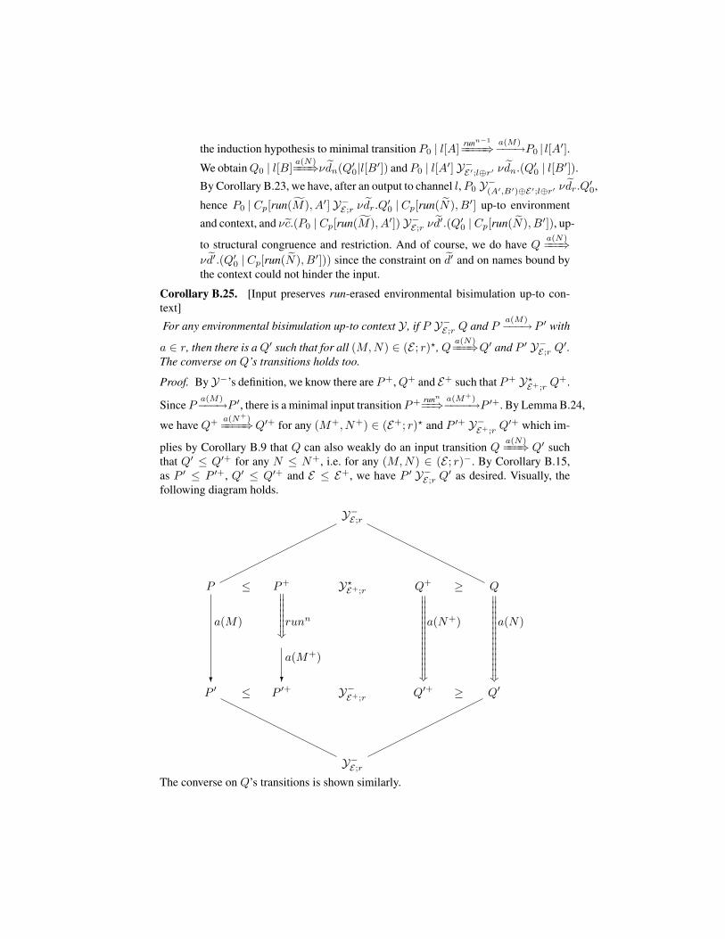
the induction hypothesis to minimal transition P0 | l[A] runn−1

====⇒ a(M)−−−→P0 | l[A′].

We obtain Q0 | l[B]a(N)===⇒νdn(Q′

0|l[B′]) and P0 | l[A′] Y−E′;l⊕r′ νdn.(Q′

0 | l[B′]).

By Corollary B.23, we have, after an output to channel l, P0 Y−(A′,B′)⊕E′;l⊕r′ νdr.Q

′0,

hence P0 | Cp[run(M), A′] Y−E;r νdr.Q

′0 | Cp[run(N), B′] up-to environment

and context, and νc.(P0 | Cp[run(M), A′]) Y−E;r νd′.(Q′

0 | Cp[run(N), B′]), up-

to structural congruence and restriction. And of course, we do have Qa(N)===⇒

νd′.(Q′0 | Cp[run(N), B′])) since the constraint on d′ and on names bound by

the context could not hinder the input.

Corollary B.25. [Input preserves run-erased environmental bisimulation up-to con-text]

For any environmental bisimulation up-to context Y , if P Y−E;r Q and P

a(M)−−−→P ′ with

a ∈ r, then there is a Q′ such that for all (M,N) ∈ (E ; r)?, Qa(N)===⇒Q′ and P ′ Y−

E;r Q′.The converse on Q’s transitions holds too.

Proof. By Y−’s definition, we know there are P+, Q+ and E+ such that P+ Y?E+;r Q+.

Since Pa(M)−−−→P ′, there is a minimal input transition P+ runn

==⇒ a(M+)−−−−→P ′+. By Lemma B.24,

we have Q+ a(N+)====⇒Q′+ for any (M+, N+) ∈ (E+; r)? and P ′+ Y−

E+;r Q′+ which im-

plies by Corollary B.9 that Q can also weakly do an input transition Qa(N)===⇒ Q′ such

that Q′ ≤ Q′+ for any N ≤ N+, i.e. for any (M,N) ∈ (E ; r)−. By Corollary B.15,as P ′ ≤ P ′+, Q′ ≤ Q′+ and E ≤ E+, we have P ′ Y−

E;r Q′ as desired. Visually, thefollowing diagram holds.

Y−E;r

P ≤ P+ Y?E+;r Q+ ≥ Q

runn�wwwwwww

P ′

a(M)

?≤ P ′+

a(M+)

?Y−E+;r Q′+

a(N+)

�

wwwwwwwwwwwwwww≥ Q′

a(N)

�

wwwwwwwwwwwwwww

Y−E;r

The converse on Q’s transitions is shown similarly.

Definition B.26. [Simple process]We define the syntax of simple processes, a subset of processes, as

Pr ::= 0 | a.Pr | a〈‘Pr〉.Pr | (Pr | Pr) | a[Pr] | !Pr | run(‘Pr)

Definition B.27. [simple environmental bisimulation up-to context]An environmental bisimulation up-to context Y is said to be simple if all of its environ-ments contain only simple processes.

Lemma B.28. [run-expanded reduction for simple environmental bisimulation up-tocontext]Suppose that P Y?

E;r Q for a simple environmental bisimulation up-to context Y , and

that Prunn

==⇒ τ−→P ′ is minimal with respect to P− τ−→P ′−, then Qτ=⇒Q′, and P ′ Y−

E;r Q′.

Proof. By induction on n.

– Case n = 0Immediate by Lemma B.20.

– Case n > 0By Lemma B.20 and Lemma B.12, we have two possible subcases preserving min-imality after the first run-transition of P

runn

==⇒ τ−→P ′.• Subcase P

run−−→ P ′′, Qτ=⇒Q′′, P ′′ Y?

E;r Q′′

We have that P ′′ runn−1

====⇒ τ−→P ′ is still minimal with respect to P− τ−→ P ′−, sowe can apply the induction hypothesis, and we are done.

• Subcase Prun−−→P ′′, Q τ=⇒Q′′, P ′′ Y−

E;r Q′′ hold, and we have P ′′ = νc.(P0 |P1)

and Q′′ = νd.(Q0 | Q1) with P0 YE′;r′ Q0, (P1, Q1) = (Cp[run(M), A],Cp[run(N), B]) ∈ (E ′; r′)−\(E ′; r′)◦, ((M ; ‘A), (N , ‘B)) ∈ E ′, {c}∩fn(E .1, r) =

{d}∩ fn(E .2, r) = ∅. Since we know P− τ−→P ′− and that Prunn

==⇒ τ−→P ′ is mini-mal with respect to it, we can infer how P weakly reduces to P ′. Let us analyseeach possibility.∗ Subsubcase A reacts with P0

Using clause 5 to add a new name l to r and clause 4 to spawn A, we haveP0 | l[A] Y?

E′;l⊕r′ Q0 | l[B]. Using an argument similar to the one in Lemma B.21,case 2, subcase 2, we know that we can apply the induction hypothe-

sis to minimal transition P0 | l[A] runn−1

====⇒ τ−→νc0.(P ′0 | l[A′]). We obtain

Q0 | l[B] τ=⇒ νd0.(Q′0 | l[B′]) and

νc0.(P ′0 | l[A′]) Y−

E′;l⊕r′ νd0.(Q′0 | l[B′]). Therefore, not only do we have

Q′′ τ=⇒ νd′.(Q′0 | Cp[ N,B′]) with {d′} = {d}∪ {d0} since the context Cp

could not bind names used in the reaction, but also byνc0.(P ′

0 | l[A′]) Y−E′;l⊕r′ νd0.(Q′

0 | l[B′]) do we have

νcr.P′0 Y−

(‘A′,B′)⊕E′;l⊕r′ νdr.Q′0 by Corollary B.23, hence

νcr.P′0 | Cp[run(M), A′] Y−

(‘A′,B′)⊕E′;l⊕r′ νdr.Q′0 | Cp[run(N), B′] up-to

context,νcr.P

′0 | Cp[run(M), A′] Y−

E;r νdr.Q′0 | Cp[run(N), B′] up-to environment,

νc0.(P ′0 | Cp[run(M), A′]) Y−

E;r νd0.(Q′0 | Cp[run(N), B′]) up-to restric-

tion and structural congruence, and finallyνc′.(P ′

0 | Cp[run(M), A′]) Y−E;r νd′.(Q′

0 | Cp[run(N), B′]) up-to restriction.∗ Subsubcase A reduces alone

Similarly, but with c′ = c and P ′0 = P0.

∗ Subsubcase A reacts with an Ai from ‘A = M (or a run-erasure of it)Let G = C[‘Ai, M

′] (resp. H = C[‘Bi, N′]) be the process of P1 (resp.

Q1) in redex position that contains Ai (resp. Bi) and reacts with the pro-cess containing A according to rule REACT-R or REACT-L. Then there isa process context C ′

p such that Cp[A, run(M)] = C ′p[A

′, G, run(M ′′)]. Byclause 5 of environmental bisimulation to add a new name l and clause 4,we have P0 | l[A] Y?

E′;l⊕r′ Q0 | l[B]. By Lemma B.16 to add a new namem to r and by up-to context, we haveP0 | l[A] |m[G] Y?

E′;m⊕l⊕r′ Q0 | l[B] |m[H].By the conditions on E ′, we know we haveP0 | l[A] |m[G] run=⇒ τ−→P0 | l[A′] |m[G′] with no name extruded.For the same reasons, when applying the induction hypothesis, we obtainQ0 | l[B] |m[H] τ=⇒ νd0.(Q′

0 | l[B′] |m[H ′]) such that there is no boundname whose scope is only B′ and H ′, as well asP0 | l[A′] |m[G′] Y−

E′;m⊕l⊕r′ νd0.(Q′0 | l[B′] |m[H ′]).

We can now passivate the contents of l[ ] and m[ ] to replace them up-tocontext, restriction and structural equivalence to getP0 | C ′

p[A′, G′, run(M ′′)] Y−

E′;m⊕l⊕r′ νd0.(Q′0 | C ′

p[B′,H ′, run(N ′′)])

and finally use up-to environment and restriction to obtainνc.(P0 | C ′

p[A′, G′, run(M ′′)]) Y−

E;r νd′.(Q′0 | C ′

p[B′,H ′, run(N ′′)]).

∗ Subsubcase A outputs and reacts with the contextLet C[M ′] (resp. C[N ′]) be the process of P1 (resp. Q1) in redex positionthat reacts with the process containing A according to rule REACT-R orREACT-L. Then there is another context C ′

p such that Cp[A, run(M)] =C ′

p[A′, C[M ′], run(M ′′)]. Using clause 5 to add a new name l to r and

clause 4 to spawn A, we haveP0 | l[A] Y?

E′;l⊕r′ Q0 | l[B].We can now apply Lemma B.22 to simulate A’s output after run-transitions,

P0 | l[A] runn−1

====⇒ a〈M〉−−−→P0 | l[A′], and we obtain

Q0 | l[B]ν ed1a〈N〉=====⇒ νd0.(Q′

0 | l[B′]), with d1’s scope encompassing Q0, andP0 | l[A′] Y−

(M,N)⊕E′;l⊕r′ νd0.(Q′0 | l[B′]) such that (M,N) belong (mod-

ulo run-erasure) to some E ′′ with no bound names or to its context closure(E ′′; r′′)?. We passivate the contents of l[ ] and haveP0 Y−

(‘A′,‘B′)⊕(M,N)⊕E′;l⊕r′ νdr.Q′0. By the restrictions on E ′, we also

know (‘A′, ‘B′) belong (modulo run-erasure) to E ′′ or to its context clo-

sure. By Lemma B.4, we have that C[M ]a(M)−−−→G and C[N ]

a(N)−−−→H with(G, H) ∈ ((M,N)⊕E ′; r′)◦. Up-to context, we build

P0 | C ′p[A

′, G, run(M ′′)] Y−(‘A′,‘B′)⊕(M,N)⊕E′;l⊕r′ νdr.Q

′0 | C ′

p[B′,H, run(N ′′)]

and then up-to environment and restrictionνc.(P0 | C ′

p[A′, G, run(M)]) Y−

E;r νd′.(Q′0 | Cp[B′,H, run(N)]).

∗ Subsubcase A inputs and reacts with the contextSuppose the context outputs a process M (resp. N ) and extrudes names x

by means of a process Co[M ′] (resp. Co[N ′]) such that Co[M ′]νex.a〈M〉−−−−−→

C ′o[M

′] (resp. Co[N ′]νex.a〈N〉−−−−−→ C ′

o[N′] by Lemma B.5). Using clause 5

several times to add a new names l and x to r and clause 4 to spawn A, wehave P0 | l[A] Y?

E′;l⊕ex⊕r′ Q0 | l[B].We can now apply Lemma B.24 to trigger A’s input of M (resp. B’s inputof N ) where x is free, after some run-transitions and we obtainP0 | l[A′] Y−

E′;l⊕ex⊕r′ νd0.(Q′0 | l[B′]).

We passivate the content of l[ ], obtainingP0 Y−

(‘A′,‘B′)⊕E′;l⊕ex⊕r′ νdr.Q′0.

Because of the constraints on input from elements of E ′, we know that xis not free in A′ nor B′. We remove l and x up-to environment from theknown names and then replace A′ and B′ up-to context, givingP0 | C ′

p[A′, run(M)] Y−

E′;r′ νdr.Q′0 | C ′

p[B′, run(N)].

Notice that, since x does not appear in A′, B′, r′ nor E ′ but could still befree in C ′

o[M′], we have the context C ′

p bind it properly around A′ andC ′

o[M′] (resp. B′ and C ′

o[N′]) as required by the reaction transition. Fi-

nally, up-to environment and restriction, we haveνc.(P0 | C ′

p[A′, run(M)]) Y−

E;r νd′.(Q′0 | Cp[B′, run(N)]) and we are done.

Corollary B.29. [Reduction preserves run-erased simple environmental bisimulationup-to context]For any simple environmental bisimulation up-to context Y , if P Y−

E;r Q and Pτ−→ P ′,

then there is a Q′ such that Qτ=⇒ Q′ and P ′ Y−

E;r Q′. The converse on Q’s transitionsholds too.

Proof. By Y−’s definition, we know there are P+, Q+ and E+ such that P+ Y?E+;r Q+.

Since Pτ−→P ′, there is a minimal reduction transition P+ runn

==⇒ τ−→P ′+. By Lemma B.28,we have Q+ τ=⇒ Q′+ and P ′+ Y−

E+;r Q′+ which implies by Corollary B.9 that Q canalso weakly reduce to some Q′ such that Q′ ≤ Q′+. By Corollary B.15, as P ′ ≤ P ′+,Q′ ≤ Q′+ and E ≤ E+, we have P ′ Y−

E;r Q′ as desired. Visually, the following diagramholds.

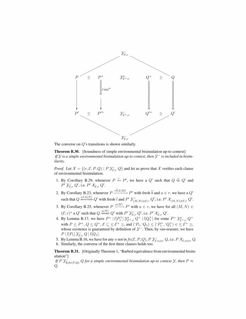
Y−E;r

P ≤ P+ Y?E+;r Q+ ≥ Q

runn�wwwwwww

P ′?

≤ P ′+?

Y−E+;r Q′+

�

wwwwwwwwwwwwwww≥ Q′

�

wwwwwwwwwwwwwww

Y−E;r

The converse on Q’s transitions is shown similarly.

Theorem B.30. [Soundness of simple environmental bisimulation up-to context]If Y is a simple environmental bisimulation up-to context, then Y− is included in bisim-ilarity.

Proof. Let X = {(r, E , P, Q) | P Y−E;r Q} and let us prove that X verifies each clause

of environmental bisimulation.

1. By Corollary B.29, whenever Pτ−→ P ′, we have a Q′ such that Q

τ=⇒ Q′ andP ′ Y−

E;r Q′, i.e. P ′ XE;r Q′.

2. By Corollary B.23, whenever Pνeb.a〈M〉−−−−−→ P ′ with fresh b and a ∈ r, we have a Q′

such that Qνec.a〈N〉=====⇒Q′ with fresh c and P ′ Y−

(M,N)⊕E;r Q′, i.e. P ′ X(M,N)⊕E;r Q′.

3. By Corollary B.25, whenever Pa(M)−−−→ P ′ with a ∈ r, we have for all (M,N) ∈

(E ; r)? a Q′ such that Qa(N)===⇒Q′ with P ′ Y−

E;r Q′, i.e. P ′ XE;r Q′.4. By Lemma B.17, we have P+ | l[P+

1 ] Y?E+;r Q+ | l[Q+

1 ] for some P+ Y?E+;r Q+

with P ≤ P+, Q ≤ Q+, E ⊆ ≤ E+ ≥, and (‘P1, ‘Q1) ≤ (‘P+1 , ‘Q+

1 ) ∈ ≤ E+ ≥,whose existence is guaranteed by definition of Y−. Then, by run-erasure, we haveP | l[P1] Y−

E;r Q | l[Q1].5. By Lemma B.16, we have for any n not in fn(E , P, Q), P Y−

E;n⊕r Q, i.e. P XE;n⊕r Q.6. Similarly, the converse of the first three clauses holds too.

Theorem B.31. [Originally Theorem 1, “Barbed equivalence from environmental bisim-ulation”]If P Y−

∅;fn(P,Q) Q for a simple environmental bisimulation up-to context Y , then P ≈Q.

Proof. We know by Theorem B.30 that Y− is an environmental bisimulation. We letZ = {(P,Q) | P Y−

∅;fn(P,Q) Q} and prove that Z is included in ≈.

1. Clause Pτ−→ P

As Y− is an environmental bisimulation, by clause 1 of the bisimulation, there isQ′ such that Q =⇒Q′ and P ′ Y−

∅;r Q′. Therefore, for r′ = fn(P ′, Q′) ⊆ r, we haveP ′ Y−

∅;r′ Q′, hence (P ′, Q′) ∈ Z .2. Clause P ↓µ

There are two cases depending on µ:– Case P ↓a

We have that Pa(V )−−−→ P ′ for some (V,W ) ∈ (∅; r)? and P ′. Since a ∈ r,

by Y− being an environmental bisimulation and clause 2 of the bisimulation,

there is also Q′ such that Qa(W )===⇒Q′, that is, Q ⇓a.

– Case P ↓a

We have that Pνec.a〈V 〉−−−−−→ P ′ for some fresh c, V , and P ′. Since a ∈ r, by Y−

being an environmental bisimulation and clause 3 of the bisimulation, there are

also W , Q′ and fresh d such that Qν ed.a〈W 〉=====⇒Q′, that is, Q ⇓a.

3. Clause Converse of 1, 2 on QSimilar to 1, 2.

4. Clause R a processLet r′ = fn(R); by appealing to the clause 5 of the bisimulation, since the namesin r′ are either fresh or already in r, we have that P Y−

∅;r∪r′ Q. Also, R (∅; r ∪ r′)◦

R and thus, using the up-to context technique, P |R Y−∅;r∪r′ Q |R since Y− is

preserved by parallel composition of processes from (∅; r ∪ r′)◦. Therefore, (P |R,Q |R) ∈ Z .

3 Reduction-closed barbed congruence from environmental bisimulations

Definition B.32. [Size of a simple process]We define inductively the size size(P ) of a simple process P as

size(P ) =

0 if P = 01 + size(Q) if P = a.Q

1 + size(Q) + size(R) if P = a〈Q〉.Rmax(size(Q), size(R)) if P = Q|R1 + size(Q) if P = l[Q]size(Q) if P = !Qsize(Q) if P = run‘Q

Notice that the size is impervious to the run constructor, and that therefore size(P ) =size(P+) for all P ≤ P+. Also, size(P ) = 0 if and only if fn(P ) = ∅.

Lemma B.33. [Size and transitions]For all simple process P , for all P ′, α, if P

α−→ P ′ then

– fn(P ) ⊇ fn(P ′).– size(P ) ≥ size(P ′). Moreover, if α = a〈‘P ′′〉, size(P ) > size(P ′′) holds too.

Proof. By induction on the transition derivations of Pα−→ P ′.

Lemma B.34. [Names and context closure]If for any (M,N) ∈ E , fn(M) = fn(N) then for any r and any (Mc, Nc) ∈ (E ; r)?,fn(Mc) = fn(Nc).

Proof. By structural induction on Mc’s context.

Lemma B.35. [Free names and simple environmental bisimulation up-to context]Let Y be a simple environmental bisimulation up-to context. If 0 YE;fn(E) 0, then for all(‘P, ‘Q) ∈ E , fn(P ) = fn(Q).

Proof. We show by induction on the size of P the contraposition: for all P , Q, E andr = fn(E), if (P,Q) ∈ E , then it holds that fn(P ) 6= fn(Q) implies (r, E , 0, 0) 6∈ Y .

– Case size(P ) = 0We know by its size that P has no free name. However, by fn(P ) 6= fn(Q), there isa name a ∈ fn(Q) such that there is a weak transition Q

run=⇒ α−→Q′ with a ∈ fn(α).Thus, if (r, E , 0, 0) ∈ Y holds, we have run(‘P ) Y?

E;r run(‘Q) by up-to context, andby Q

run=⇒ α−→ (hence run(‘Q) run=⇒ α−→) and Lemma B.22 or Lemma B.24 we shouldhave run(‘P ) α=⇒. However, by Lemma B.33, P will never weakly exhibit α and wethus reached a contradiction, hence (r, E , 0, 0) 6∈ Y .

– Case size(P ) > 0Assuming fn(P ) > fn(Q), we know there is a name a ∈ fn(P ) \ fn(Q) such thatone of the two following cases holds.1. P

α1−→ . . .αn−−→ o〈M〉−−−→ with a ∈ fn(M).

Suppose 0 YE;r 0, we have l[P ] Y?E;l⊕r l[Q] for some l not in r by clauses 5

and 4 of environmental bisimulation up-to context. Then, we have l[P ] α1−→. . .

αn−−→ o〈M〉−−−→l[P ′], hence l[Q] α1=⇒ . . .αn=⇒ o〈N〉

===⇒l[Q′], with a 6∈ fn(N) byLemma B.35 and l[P ′] Y−

(M,N)⊕...⊕E;l⊕r l[Q′]. By Lemma B.33 we know thatsize(M) < size(P). By Corollary B.23, we have 0 Y−

(‘P ′,‘Q′)⊕(M,N)⊕...⊕E;r 0.Therefore, we also have an E ′ such that (‘P ′+, ‘Q′+)⊕(M+, N+)⊕ . . .⊕E ⊆(E ′; r)? with (M,N) ≤ (M+, N+). There is therefore a pair of terms (‘Pm, ‘Qm) ∈E ′ such that (M+, N+) = (C[‘A, ‘Pm], C[‘B, ‘Qn]) and fn(Pm) 6= fn(Qm).Naturally, by size(M+) = size(M) < size(P ), we have size(Pm) < size(P ).We thus apply the induction hypothesis to Pm and E ′, and obtain that (r, E ′, 0, 0) 6∈Y . Therefore, (r, (‘P ′+, ‘Q′+)⊕(M+, N+)⊕ . . .⊕E , 0, 0) 6∈ Y?, hence(r, (‘P ′, ‘Q′)⊕(M,N)⊕ . . .⊕E , 0, 0) 6∈ Y−. However, (r, (‘P ′, ‘Q′)⊕(M,N)⊕. . .⊕E , 0, 0) ∈ Y− was a requirement from (r, E , 0, 0) ∈ Y which thereforedoes not hold.

2. Either Pα1−→ . . .

αn−−→ a〈·〉−−→ or Pα1−→ . . .

αn−−→ a−→.Assuming 0 YE;r 0, we have l[P ] Y?

E;r l[Q] and Pα1−→ . . .

αn−−→ P ′ α−→ with α =a〈·〉 or α = a, hence Q

α1=⇒ . . .αn=⇒ Q′, but, by Lemma B.33, we do not have

Q′ α=⇒, which contradicts 0 YE;r 0.

The situation fn(P ) < fn(Q) is handled similarly.

Lemma B.36. [Barbed congruence from run-erasure and simple environmental bisim-ulation up-to context]Let Y be the simple environmental bisimilarity up-to context, and S = {(P,Q) | P ≤C[P+], Q ≤ C[Q+], ∃E .(P+, Q+) ∈ E , 0 Y

E;fn( eP+, eQ+)0}, for contexts C for pro-

cesses. We show that for all closed (P,Q) ∈ S, if P ↓µ then Q ⇓µ, and that if P −→ P ′

then Q =⇒Q′ for some Q′ with (P ′, Q′) ∈ S, and conversely.

Proof. By induction on the transition derivation of Pα−→ P ′ with (P,Q) ∈ S. We

prove the two properties separately. In both situations, there is a case analysis on whodoes the transition: the context’s erasure or some Pi. By symmetricity, we do not showthe converse proofs on Q’s transition; they are similar. We write run∗‘(P ) to meanrun‘(. . . (run‘(P )) . . . ), and C−

p , C−q for two possibly different erasures of the same C.

Barbs: the cases necessary to check for barbs are HO-IN, HO-OUT, PAR-R, PAR-L,REP, EXTR, GUARD, TRANSP, and PASSIV.

– HO-IN

• Subcase C−p [P ] = a(X).C−

1p[P ]

If C−p [P ] ↓a, we have a(X).C−

1p[P ]a(M)−−−→·. Thus C−

q [Q] = run∗‘(a(X).C−1q[Q])

run=⇒ a(X).C−1q[Q])

a(N)−−−→ ·, i.e. C−q [Q] ⇓a

• Subcase [ ]iBy (r, E , 0, 0) ∈ Y , we have Pi Y−

E;r Qi, hence Qi ⇓a if Pi ↓a, hence run∗‘Qi ⇓a,that is C−

p [Q] ⇓a.– HO-OUT

• Subcase C−p [P ] = a〈D−

p [P ]〉.C−1p[P ]

If C−p [P ] ↓a, we have a〈‘D−

p [P ]〉.C−1p[P ]

a〈‘D−p [ eP ]〉

−−−−−−→ ·. Thus, C−q [Q] =

run∗‘(a〈‘D−p [Q]〉.C−

1q[Q]) run=⇒ a〈‘D−p [Q]〉.C−

1q[Q])a〈‘D−

p [ eQ]〉−−−−−−→ · i.e. C−

q [Q] ⇓a

• Subcase [ ]iBy (r, E , 0, 0) ∈ Y , we have Pi Y−

E;r Qi, hence Qi ⇓a if Pi ↓a, hence run∗‘Qi ⇓a,that is C−

p [Q] ⇓a.In all the other cases, this subcase is similar, and we will thus not write it any-more.

– PASSIVC−

p [P ] = a[C−1p[P ]] ↓a. Trivially a[C−

1q[Q]] ↓a, hence C−q [Q] = run∗‘(a[C−

1q[Q]]) ⇓a.– PAR-L

C−p [P ] = C−

1p[P ] | C−2p[P ] ↓µ hence C−

1p[P ] ↓µ. By the induction hypothesis,C−

1q[Q] ⇓µ hence C−q [Q] = run∗‘(C−

1q[Q] | C−2q[Q]) ⇓µ.

– PAR-RSimilarly.

– REPC−

p [P ] = !C−1p[P ] ↓µ, hence !C−

1p[P ] | C−1p[P ] ↓µ. By the induction hypothesis,

!C−1q[Q] | C−

1q[Q] ⇓µ, hence C−q [Q] = run∗‘(!C−

1q[Q]) ⇓µ.

– EXTRC−

p [P ] = νx.C−1p[P ] ↓µ, hence C−

1p[P ] ↓µ. By the induction hypothesis, C−1q[Q] ⇓µ,

hence νx.C−1q[Q] ⇓µ since the same barb µ 6= x, x is used, hence C−

q [Q] =run∗‘(νx.C−

1q[Q]) ⇓µ.– GUARD

Similarly.– TRANSP

C−p [P ] = a[C−

1p[P ]] ↓µ, hence C−1p[P ] ↓µ. By the induction hypothesis, C−

1q[Q] ⇓µ,hence a[C−

1q[Q]] ⇓µ, hence C−q [Q] = run∗‘(a[C−

1q[Q]]) ⇓µ.

Reductions: the cases necessary to check for reduction closure are RUN, TRANSP,PAR-L, PAR-R, REP, GUARD, REACT-L, and REACT-R.

– RUN

• run(‘C−1p[P ])−→ C−

1p[P ]We have run(‘C−

1p[P ])−→C−1p[P ] and C−

1p[P ] ≤ C[P+]. We still have C−q [Q] ≤

C[Q+], so (P ′, Q) ∈ S and we are done.• [ ]i

We have a[Pi] Y−E;r a[Qi] and a[Pi]−→a[P ′

i ]a〈‘P ′

i 〉−−−−→0, so a[Qi]=⇒a[Q′i]

a〈‘Qi〉====⇒0,and 0 Y−

(‘P ′i ,‘Q′

i)⊕E;r 0, hence (P ′i , Q

′i) ∈ S. Also, run∗(‘Qi) =⇒ Qi =⇒ Q′

i andwe are done.

– TRANSP

• a[C−1p[P ]]−→ a[R]

We have C−1p[P ]−→R, so, by the induction hypothesis C−

1q[Q]=⇒S and (R,S) ∈S. Therefore a[C−

1q[Q]] =⇒ a[S], and (a[R], a[S]) ∈ S• [ ]i

We have a[Pi] Y−E;r a[Qi] a[Pi]−→ a[P ′

i ]a〈‘P ′

i 〉−−−−→ 0. So, a[Qi] =⇒ a[Q′i]

a〈‘Q′i〉====⇒ 0,

and 0 Y−(‘P ′

i ,‘Q′i)⊕E;r 0, hence (a[P ′

i ], a[Q′i]) ∈ S. Also, run∗(‘Qi) =⇒Qi =⇒Q′

i

and we are done. Again, this subcase always holds similarly, and thus it is notrepeated below.

– PAR-LC−

p [P ] = C−1p[P ] | C−

2p[P ] −→ R | C−2p[P ], i.e. C−

1p[P ] −→ R. So, by the inductionhypothesis, C−

1q[Q]=⇒S and (R,S) ∈ S, hence C−q [Q] = run∗‘(C−

1q[Q]|C−2q[Q])=⇒

S | C−2q[Q] and (R | C−

2p[P ], S | C−2q[Q]) ∈ S.

– PAR-RSimilarly

– REPC−

p [P ] = !C−1p[P ] −→ R, hence !C−

1p[P ] | C−1p[P ] −→ R. By the induction hypoth-

esis, !C−1q[Q] | C−

1q[Q] =⇒ S with (R,S) ∈ S, hence, !C−1q[Q] =⇒ S, C−

q [Q] =run∗‘(!C−

1q[Q]) =⇒ S, and still (R,S) ∈ S.– GUARD

C−p [P ] = νx.C−

1p[P ] −→ νx.R, i.e. C−1p[P ] −→ R. So, by the induction hypothesis,

C−1q[Q]=⇒S and (R,S) ∈ S hence vx.C−

1q[Q]=⇒vx.S, C−q [Q] = run∗‘(νx.C−

1q[Q])=⇒νx.S and (νx.R, νx.S) ∈ S.

– REACT-LThere are several subcases.

• The two contexts reactC−

p [P ] = C−1p[P0, P1] | C−

2p[P2] −→ νx.(C ′−1p [P0] | C ′−

2p [P2, P1]). Of course,C−

1qcan (weakly) do the same reaction, and since fn(P1) = fn(Q1) by Lemma B.35,the same names x are extruded, giving C−

q [Q] =⇒ νx.(C ′−1q [Q0] |C ′−

2q [Q2, Q1])and as expected (νx.(C ′−

1p [P0] |C ′−2p [P2, P1]), νx.(C ′−

1q [Q0] |C ′−2q [Q2, Q1])) ∈

S.• C−

1p[P1] sends, Pi in C−2p[P2, Pi] receives.

C−p [P ] = C−

1p[P1] | C−2p[P2, Pi]−→ νx.(C ′−

1p [P1] | C ′−2p [P2, P

′i ]). We know that

C−1q[Q] can weakly do the same output transition, that it will extrude the same

names. Also, we have a[Pi] Y−E;r a[Qi] and a[Pi]

o−→ a[P ′i ]

a〈‘P ′i 〉−−−−→ 0 for some

channel o ∈ r. So, a[Qi]o=⇒a[Q′

i]a〈‘Q′

i〉−−−−→0 with (r, (‘P ′i , ‘Q

′i)⊕E , 0, 0) ∈ Y−, so

C−q [Q]=⇒νx.(C ′−

1q [Q1]|C ′−2q [Q2, Q

′i]), and (νx.(C ′−

1p [P1]|C ′−2p [P2, P

′i ]), νx.(C ′−

1q [Q1]|C ′−

2q [Q2, Q′i])) ∈ S.

• C−2p[P2] receives, Pi in C−

1p[P1, Pi] sendsC−

p [P ] = C−1p[P1, Pi]|C−

2p[P2]−→νx.(C ′−1p [P1, P

′i ]|C

−2p[P2, Pj ]). We know that

C−2q[Q2] can weakly do the same input transition. Also, we have a[Pi] Y−

E;r a[Qi]

and a[Pi]o〈‘Pj〉−−−−→ a[P ′

i ]a〈‘P ′

i 〉−−−−→ 0, so, a[Qi]o〈‘Qj〉====⇒ a[Q′

i]a〈‘Q′

i〉−−−−→ 0 with(r, (‘Pj , ‘Qj)⊕(‘P ′

i , ‘Q′i)⊕E , 0, 0) ∈ Y− and the same names in (Pj , Qj) by

Lemma B.35, so C−q [Q]=⇒νx.(C ′−

1q [Q1, Q′i]|C

′−2q [Q2, Qj ]), and (νx.(C ′−

1p [P1, P′i ]|

C ′−2p [P2, Pj ]), νx.(C ′−

1q [Q1, Q′i] | C

′−2q [Q2, Qj ])) ∈ S.

• Pi in C−1p[P1, Pi] and Pj in C−

2p[P2, Pj ] reactC−

p [P ] = C−1p[P1, Pi] |C−

2p[P2, Pj ]−→νx.(C ′−1p [P1, P

′i ] |C

−2p[P2, P

′j ]). We have

a[Pi] | b[Pj ] Y−E;r a[Qi] | b[Qj ] and a[Pi] |b[Pj ]−→a[P ′

i ] |b[P ′j ]

a〈‘P ′i 〉−−−−→

b〈‘P ′j〉−−−−→0,

so a[Qi]|b[Qj ]=⇒a[Q′i]|b[Q′

j ]a〈‘Q′

i〉−−−−→b〈‘Q′

j〉−−−−→0 with (r, (‘P ′j , ‘Q

′j)⊕(‘P ′

i , ‘Q′i)⊕E , 0, 0) ∈

Y− and the same names communicated from Pi, Qi to Pj , Qj by Lemma B.35,so C−

q [Q]=⇒νx.(C ′−1q [Q1, Q

′i]|C

′−2q [Q2, Q

′j ]), and (νx.(C ′−

1p [P1, P′i ]|C

′−2p [P2, P

′j ]),

νx.(C ′−1q [Q1, Q

′i] | C

′−2q [Q2, Q

′j ])) ∈ S

– REACT-RSimilarly

Corollary B.37. [Originally Corollary 1, “Barbed congruence from environmentalbisimulation”]If a〈‘P 〉 Y−

∅;a⊕fn(P,Q) a〈‘Q〉 for a simple environmental bisimulation up-to context Y ,then P ≈c Q.

Proof. By a〈‘P 〉 Y∅;a⊕fn(P,Q) a〈‘Q〉, we have 0 Y?(‘P,‘Q);a⊕fn(P,Q) 0, hence 0 YE;r 0

for an environment E and names r such that (‘P, ‘Q) ∈ (E ; r)? and a⊕fn(‘P, ‘Q) ⊆ r.By Lemma B.36, we have (P,Q) ∈ S, for some S included in ≈c.

C Examples

We write P | . . . | P for a finite, possibly null, product of the process P .

Example C.1. [Originally Example 2]!a | !e ≈ !a[e].

Proof. Take X = {(r, E , P, Q) | r ⊇ {a, e, l1, . . . , ln} | E = {(‘0, ‘e)}, n ≥ 0,P = !a | !e |

∏ni=1 li[0], Q = !a[e] |

∏ni=1 li[e] | a[0] | . . . | a[0]}. As expected, the

definition ofX relates the original processes !a|!e and !a[e]. Clause 4 of the bisimulationrequires that for any (‘P1, ‘Q1) ∈ E and l ∈ r, we have P0 | l[P1] XE;r Q0 | l[Q1].Repeatedly applying this clause explains the presence of the products

∏ni=1 li[·] in both

P and Q. All outputs that P and Q can do are respectively {‘0} and {‘0, ‘e}. However,since (‘0, ‘0) ∈ ({(‘0, ‘e)}; ∅)?, we can work up-to context with smaller environmentE = {(‘0, ‘e)}. Finally, at least the free names a, e, l1, . . . , ln of P and Q and maybemore fresh names are in r, so to satisfy clause 5 of the bisimulation and to guaranteebehavioural equivalence.

Let us now check the output clause of the bisimulation, starting with passivation ofli[·] which is trivial to verify since all output terms are already related by E . Otherwise,

P can only output by doing Pa〈‘0〉−−−→≡P , and Q can follow with Q

a〈‘e〉−−−→≡Q with still(r, E , P, Q) ∈ X . Conversely, when Q outputs to a either ‘0 or ‘e, P follows with anaction a〈‘0〉 from a replication of a, and we are done.

As far as inputs are concerned, whenever Pe−→≡P , Q can consume the e in a copy of

a[e] to become a process Q|a[0] (hence the list a[0]|. . .|a[0]), which is still related byXto P under r and E . The converse transition is treated similarly. Q can also input in li[e]with a transition li[e]

e−→ li[0], in which case P can input on a replication from !e, doingP

e−→≡P . We can remove up-to context the ln[0] of Q’s transition and P ’s original ln[0],and we are done since (r, E , !a | !e |

∏n−1i=1 li[0], !a[e] |

∏n−1i=1 li[e] | a[0] | . . . | a[0]) ∈ X .

Without loss of generality, internal transitions involve passivation of ln[·] (necessar-ily with ln = e), and are easily matched: (i) when P = !a | !e |

∏ni=1 li[0] τ−→≡ !a | !e |∏n−1

i=1 li[0], Q can do !a[e] |∏n

i=1 li[e] |a[0] | . . . |a[0] τ−→≡ !a[e] |∏n−1

i=1 li[e] |a[0] |a[0] |. . . | a[0] (which increases the count of a[0]’s); (ii) the converse of (i) by Q is similar,and (iii) when Q = !a[e] |

∏n−2i=1 li[e] | ln−1[e] | ln[e] τ−→≡ !a[e] |

∏n−2i=1 li[e] | ln−1[0], P

can passivate ln[0] using a replication from !e. The resulting processes are still relatedby X with r and E , and we can even remove the ln−1[0]’s up-to context.

We therefore have !a | !e ≈ !a[e] from the soundness of environmental bisimulationup-to context.

Example C.2. [Originally Example 3]!a[e]|!b[e] ≈ !a[b[e|e]]. This example shows the equivalence proof of more complicatedprocesses with nested locations.

Proof. Take:

X = {(r, E , P, Q) | r ⊇ {a, e, b, l1, . . . , ln},P0 = !a[e] | !b[e], Q0 = !a[b[e | e]],P = P0 |

∏ni=1 li[Pi] | b[0] | . . . | b[0],

Q = Q0 |∏n

i=1 li[Qi],(P , Q) ∈ E , n ≥ 0},

E = {(‘x, ‘y) | x ∈ {0, e, e}, y ≡∈ {0, e, e, (e | e), b[0], b[e], b[e], b[e | e]}} .

X relates considered processes P0 and Q0 together with a set r containing at leastthe free names of P and Q, and an environment E defined as the Cartesian product ofall terms that we expect P and Q to output. As in Examples 1 and C.1, we could omitpairs of the form (‘x, ‘x) from E , but this would only complicate the definition. As inExample C.1, we have the products

∏ni=1 li[·] by clause 4 of the bisimulation. Process

P may also contain a list of subprocesses b[0] | . . . |b[0] whose presence will be clarifiedbelow.

Let us now check the input transitions. When P inputs on e, it either uses a copy ofa[e], leaving behind a[0], or uses Pn which becomes P ′

n. Q0 too can input on e, leavinga process a[b[e]]. Then, in the former case, a[0] and a[b[e]] can be merged with theproducts

∏since (‘0, ‘b[e]) ∈ E . Else, in the latter case, it holds that (‘P ′

n, ‘Qn) ∈ E ;we can then draw a copy a[e] from P0 and, since (‘e, ‘b[e]) ∈ E too, we can merge Q’sresidue a[b[e]] and the copy a[e] with their corresponding products

∏. Finally, inputs

by Q are matched similarly. From now on, we shall refer as pairing to the drawing fromP0 or Q0 of a process to pair with a residue so to enlarge the products

∏.

Outputs transitions are conceptually matched similarly: when P0e−→P0 |b[0], process

Q can follow with Q0e−→≡Q0 | a[b[e]] (and conversely), but b[0] and a[b[e]] cannot be

added together to the products∏

, for locations a and b differ. Yet, we can use pairing tohandle a[b[e]], and leave the residue b[0] as is, therefore enlarging the list b[0]|. . .|b[0] inP . Outputs by Pn (resp. Qn) are matched in a similar manner: output with a copy fromQ0 (resp. P0) leaving a residue a[·], and pairing to handle this residue. Passivations ofli[·] and a[·] are trivial to simulate, since (‘Pi, ‘Qi) and (‘e, ‘b[e|e]) are in E . Passivationsof P ’s b[e] and b[0] are matched by the passivation of b[e |e] in a replication drawn fromQ0, leaving a residue a[0] paired as usual. Passivation of Q0’s b[e|e] is handled similarly.

Finally, when Qnb〈‘R〉−−−→Q′

n = 0 for R ∈ {0, e, e, (e | e)}, we can just passivate a copyof b[e] from P0 and we are done since (‘e, ‘R) and (‘Pn, ‘0) are both in the environmentE .

We now check the τ transitions clause. If P0 reduces to P0 | a[0] | b[0], or reactswith Pi leaving residues a[0] or b[0], we use pairing for the a[0]’s, and add the b[0]’sto b[0] | . . . | b[0]. Conversely, Q0 can reduce to Q0 | a[b[0]] or Q0 | a[b[e]] | a[b[e]],or may react with Qi, leaving residues a[b[e]] or a[b[e]]. All residues can be paired upwith one or two copies of a[e] from P0, and in all the above reactions, integrity ofthe products is preserved (i.e. (‘P , ‘Q) ∈ E still holds). Also, ln[·] can be passivated(necessarily with ln = e) in P by either a[e] or Pn−1. Therefore P becomes eitherP0 | a[0] |

∏n−1i=1 li[Pi] | b[0] | . . . | b[0] or P0 |

∏n−2i=1 li[Pi] | ln−1[P ′

n−1] | b[0] | . . . | b[0].In both cases, Q follows with Q

τ−→≡ Q0 | a[b[e]] |∏n−1

i=1 li[Qi], and either a[0] and

a[b[e]] join the products∏

, or pairing is used to assure membership in X . The conversefor Q of those reactions with a passivation is similarly checked. Finally, for reactionsinvolving only Pi’s (resp. Qi’s), Q (resp. P ) needs not do anything, for the integrity ofthe products

∏is preserved.

This concludes our proof that the original processes !a[e] | !b[e] and !a[b[e | e]] arebehaviourally equivalent.