SOPHISTICATED VS. SIMPLE SYSTEMIC

RISK MEASURES DAVID PANKOKE

WORKING PAPERS ON RISK MANAGEMENT AND INSURANCE NO. 157

EDITED BY HATO SCHMEISER

CHAIR FOR RISK MANAGEMENT AND

INSURANCE

DECEMBER 2014

Sophisticated vs. Simple Systemic Risk Measures*

David Pankoke†

December 12, 2014

Abstract: This paper evaluates whether sophisticated or simple systemic risk measures are

more suitable in identifying which institutions contribute to systemic risk. In this

investigation, CoVaR, Marginal Expected Shortfall (MES), SRISK and Granger-Causality

Networks are considered as sophisticated systemic risk measures. Market capitalization, total

debt, leverage, the stock market returns of an institution, and the correlation between the stock

market returns of an institution and the market, are considered as simple systemic risk

measures. Systemic relevance is approximated by the receipt of financial support during the

financial crisis and the classification, as a systemically important institution, by national or

international regulators. The analyses are performed for all companies included in the S&P

500 composite index. The findings suggest that simple systemic risk measures have more

explanatory power than sophisticated risk measures. In particular, total debt is found to be the

most suitable indicator to detect institutions which contribute to systemic risk, according to

the explanatory power and model fit. The most suitable sophisticated risk measure seems to

be SRISK.

Keywords: Systemic Risk, CoVaR, Marginal Expected Shortfall, SRISK, Granger-

Causality Networks

* I am very grateful for the helpful comments I received from Semir Ben Ammar, Martin Eling, Felix

Irresberger, Stefan Legge, Philipp Schaper and Florian Schreiber. I am also grateful for the participant discussions at the annual conference of the Asia-Pacific Risk and Insurance Association (APRIA) in 2014, the annual meeting of the American Risk and Insurance Association (ARIA) in 2014 and the annual seminar of the European Group of Risk and Insurance Economists (EGRIE) in 2014. All errors and shortcomings of the paper are my own.

† David Pankoke (david.pankoke@unisg.ch) is with the Institute of Insurance Economics, University of St. Gallen, Kirchlistrassse 2, 9000 St. Gallen, Switzerland.

1

1. Introduction

In the aftermath of the financial crisis of 2008, a wholly new strand of literature emerged with

the goal of measuring systemic risk.1 These measures can broadly be divided into two

categories: (1) macroprudential measures with the goal of measuring the systemic risk of the

entire financial system, and (2) microprudential measures which have the goal of identifying

the individual contribution of companies to the overall systemic risk of the financial system.

The four most relevant sophisticated microprudential measures are: CoVaR (Adrian and

Brunnermeier, 2011), Marginal Expected Shortfall (MES) (Acharya et al., 2010; Corvasce,

2013), SRISK (Acharya et al., 2012),2 and Granger-Causality Networks (Billio et al., 2012).3

Besides these attempts to develop systemic risk measures, there is also the contrasting view in

in the literature that systemic risk measures, with an increasing degree of sophistication, have

some shortfalls. More specifically, the application of sophisticated systemic risk measures is

difficult; hence, they lack transparency (Drehmann and Tarashev, 2011). Therefore,

sophisticated measures might not necessarily be the best choice for identifying and regulating

systemically relevant institutions. Consequently, simple measures might be more suitable

(see, for example, Pottier and Sommer, 2002; Drehmann and Tarashev, 2011; Haldane, 2012;

Patro et al., 2013; Rodríguez-Moreno and Peña, 2013).

This paper evaluates whether sophisticated or simple systemic risk measures are more suitable

in indicating which companies contribute to systemic risk. In a first approach, I examine the

explanatory power of various measures with respect to governmental support received during

the financial crisis of 2008. My analysis is based on U.S. companies listed in the S&P 500

composite index in 2007. In a second approach, I investigate which measures correctly predict

companies that were recently labeled systemically important. The analysis is based on U.S.

companies listed in the S&P 500 composite index in 2013.

The contribution of this paper is threefold. Firstly, this is the first empirical comparison of

sophisticated and simple systemic risk measures by means of a benchmark approximating

systemic risk. Other studies usually either only provide rankings (Rodríguez-Moreno and

Peña, 2013; Huang et al., 2012) or only test sophisticated systemic risk measures (Idier et al.,

1 An overview of the various measures is provided by Bisias et al. (2012). 2 SRISK is not an acronym, but the name of the systemic risk measure indicating how much capital a company

needs in a future crisis. 3 According to Neale (2012), Benoit et al. (2013), Balla et al. (2014), Eling and Pankoke (2014) and Jobst

(2014), CoVaR, MES, SRISK and Granger-Causality Networks are the most widely used systemic risk measures; hence, this is why I focus on these measures in this paper.

2

2013).4 Secondly, to the best of my knowledge, this is the first study using a heterogeneous

and large sample in the context of systemic risk measures.5 This carries the advantage that

companies are included in the analyses, which are not banks, but which can still be

systemically important (e.g., AIG).6 Thirdly, this paper is the first using information about

which companies received financial support during the financial crisis and information about

the classification of institutions by regulators to evaluate the usefulness of systemic risk

measures. So far, there have only been a few papers that tested systemic risk measures in a

way other than by the measure’s ability to forecast the company’s stock market returns.7

There are two basic assumptions made in this paper. The first is that, during the financial

crisis, as well as during the present time, regulators have been able to detect the institutions

which are contributing to systemic risk. The second is that microprudential risk measures are

independent of the general state of the system. The idea to use the regulator’s point of view in

a regression analysis as the dependent variable is first mentioned by Benoit et al. (2013), but

has not yet been implemented.8 The first study using the information about which institutions

received financial support to approximate systemic risk is Weiß and Mühlnickel (2014). The

second assumption is generally implicitly made in the literature. For example, none of the

previously mentioned systemic risk measures are sensitive to the market context in the sense

that it takes feedback effects into account. Whether the stock market is in a slump or booming

it has no impact on the methodology of the measures.

The primary empirical findings are as follows. 1) Simple systemic risk measures have more

explanatory power than sophisticated ones, in determining the institutions which received

financial support during the financial crisis. In addition, they can better explain the amount of

4 As additional examples, each paper introducing a new systemic risk measure can be named. Normally, each

paper introduces a new concept for measuring systemic risk and presents a small empirical implementation, which should prove the superiority of the systemic risk measure at hand. Alternative sophisticated or simple systemic risk measures are usually ignored (see, e.g., Huang et al., 2009; Acharya et al., 2010; Adrian and Brunnermeier, 2011; Billio et al., 2012).

5 Recent studies only consider very small sample sizes. For example, Calice et al. (2012) focus on 16 banks form the U.S. and Europe, Patro et al. (2013) only consider 22 U.S. banks, Balla et al. (2014) consider 29 U.S. depositories and Papanikolaou and Wolff (2014) focus on 20 U.S. banks.

6 The financial crisis has been caused by institutions of the financial sector (see, e.g., Gorton and Metrick, 2012). Consequently, systemic risk measures should indicate companies belonging to this sector. However, one cannot only focus on the financial sector, since a few companies from other sectors, like General Electric (see, e.g., Katz, 2013), are also highly contributing to systemic risk.

7 An exception is the study by Duca and Peltonen (2013). They use a dependent variable in their regressions based on a financial stress index. As explanatory variables, they use macroprudential systemic risk indicators as GDP growth, inflation and the current account deficit of a country.

8 Furthermore, in a comment by DeYoung (2012) about the paper of Calice et al. (2012) he uses the receivement of TARP funds as a sanity check and asks: “Are these point estimates consistent with our knowledge of how these large banks fared during the financial crisis?”

3

financial support each company received. 2) Simple systemic risk measures have more

explanatory power than sophisticated ones, in determining which institutions are currently

considered systemically relevant by national or international regulators. 3) The size of a

company and its total debt level are the most suitable indicators to determine the systemic risk

contribution of an institution. The explanatory power of the size variables is higher than the

one of leverage, stock market returns or correlation variables. 4) Among the sophisticated risk

measures, SRISK seems to be the most suitable, since it has explanatory power in various

model settings; in comparison to the other sophisticated risk measures, it is the most

significant.

The rest of the paper is structured as follows. Section 2 explains the methodology, including

the sophisticated and simple systemic risk measures. Section 3 describes the data. Section 4

discusses the results. Finally, Section 5 concludes and further research questions are

discussed.

4

2. Methodology

This paper empirically evaluates whether sophisticated or simple systemic risk measures are

more suitable to identify institutions which contribute to systemic risk. Therefore, I regress

the systemic relevance of institutions on sophisticated and simple systemic risk measures. The

suitability of measures is finally interpreted according to the significance of the results and the

model fit.

The systemic relevance of companies is approximated via two different approaches. The first

approach focuses on the receipt of financial support during the financial crisis and leads to

two different dependent variables. A dichotomous variable is created by taking into account

whether financial support is received, and a cardinal variable, by focusing on the amount of

received financial support. The second approach takes into account the institutions which are

classified as systemically important institutions (SII) in 2013 and leads to a dichotomous

variable.9 Consequently, there will be two dummy variables approximating systemic

relevance: the reception of financial support and the classification as SII by national or

international supervisors. The extent of the systemic relevance of an institution will be

approximated by the amount of financial support the institution received. These three

variables are used as dependent variables in the regression analyses. This approach follows

Weiß and Mühlnickel (2014, p. 109), who “define the most systemically important insurers as

those companies that required aid under TARP [Troubled Asset Relief Program]”.10

For the first approach, the following programs are considered, all of which target individual

institutions to ensure financial stability or to reduce systemic risk:11 TARP, Temporary

Liquidity Guarantee Program (TLGP), Maiden Lane I, II, III, AIG Revolving Credit Facility

and Securities Borrowing Facility for AIG.

The second approach, and the selection of the SIIs, is based on the Financial Stability Board’s

(FSB) designations of global systemically important banks and global systemically important

insurers, as well as on the U.S. Financial Stability Oversight Council’s (FSOC) designations

of Nonbank Financial Companies and Financial Market Utilities, which are systemically

9 Two different samples are used in the analyses. The first approach is based on the companies included in the

S&P 500 composite index as of January 2007. The second approach is based on S&P 500 companies as well, but in contrast, as a reference point, January 2013 is considered.

10 In addition, see Papanikolaou and Wolff (2014) who relate the participation in TARP of an institution to systemic risk as well.

11 See Congress of the U.S. (2008, Sec 2 [1]), Federal Deposit Insurance Corporation (2008) and Federal Reserve System (2014).

5

important.12 The participation in the Comprehensive Capital Analysis and Review by the

Federal Reserve Board is not considered an indicator for systemic relevance, because only the

50 largest banks are considered in the review. An inclusion would have led to problems of

endogeneity.

As mentioned previously, there is a variety of microprudential sophisticated systemic risk

measures. In this paper, CoVaR, MES, SRISK and Granger Causality Networks are applied,

since they are considered the most relevant by the literature. In addition, they cover a wide

field of different approaches to systemic risk (Neale, 2012; Benoit et al., 2013; Balla et al.,

2014; Eling and Pankoke, 2014; Jobst, 2014)

The simple systemic risk measures used in this paper are motivated by Haldane (2012), in the

case of leverage, as well as by Drehmann and Tarashev (2011), in the case of size. Another

reason why size has to be included in the analyses is provided by the too-big-to-fail (TBTF)

literature. Brewer III and Jagtiani (2013) for example examine mergers of banks in the U.S.

between 1991 and 2004 and define a TBTF institution as one with total book value assets in

excess of $100 billion. They find that between $15 billion and $23 billion premiums have

been paid more for mergers which resulted in a TBTF institution than for mergers which

resulted in smaller companies. Therefore, markets assume implicitly that size determines

systemic risk, because TBTF institutions are only bailed out due to their impact on financial

stability.13 The motivation for using stock market returns as a simple systemic risk measure is

based on the calculation of MES (Acharya et al., 2010). The MES of a company considers the

stock market returns, but only considers the returns of a company when the entire market is in

a slump. However, previous studies have not tested if the “tail returns” considered by MES do

have more explanatory power ex ante than stock market returns. The same logic applies to the

linear correlation between the stock market returns of a company and the returns of the entire

market. Many researchers argue that correlation should play an important part in the design of

any systemic risk measure. For example, Billio et al. (2012) and Chen et al. (2014) use

Granger-Causality Networks to access systemic risk. In particular, Balla et al. (2014) argue

that the tail correlations between different entities should be considered. The Pearson

12 See FSB (2013a), FSB (2013b) and FSOC (2013). The FSB is an international organization that was

established by the G-20 in April 2009. Its purpose is to monitor the finance industry and to make recommendations for addressing systemic risk. The FSOC is a committee chaired by the U.S. Secretary of the Treasury and an insurance expert appointed by the U.S. President. Its purpose is to identify threats to the stability of the financial system.

13 See Brewer III and Jagtiani (2013) for additional evidence that TBTF institutions are only bailed out because of their impact on financial stability.

6

correlation should not be such a good indicator since the goal is to focus on spillover effects

and not to focus on general co-movements in the market. Nevertheless, Patro et al. (2013)

propose the Pearson correlation as a simple systemic risk measure. In an empirical application

they show for 22 large U.S. banks that during times of crisis overall correlation spikes and

seems to be a useful systemic risk measure.

An overview of the variables and their expected relationships can be found in Table 1.

Detailed descriptions of the systemic risk measures can be found in Sections 2.1, 2.2, 2.3 and

2.4. The regression models are illustrated in Section 2.5.

7

Explanation Rationale

Dependent Variables First Approach

Support Dichotomous variable. One, if the company received financial support in 2008, otherwise zero.

Goal of financial support is to ensure financial stability (see, e.g, Congress of the U.S., 2008, Sec 2 [1]).

Amount Continuous variable. Amount of received financial support in million USD in 2008.

Goal of financial support is to ensure financial stability (see, e.g, Congress of the U.S., 2008, Sec 2 [1]).

Second Approach

SII Dichotomous variable. One, if company is classified as systemically important in 2013, otherwise zero.

Goal of classification is to indicate institutions which can contribute to a systemic crisis (see, e.g., IAIS, 2013, p. 6).

Independent Variables - Sophisticated Systemic Risk Measures

CoVaR

Systemic risk measure which considers the entire contribution of a company to systemic risk (Section 2.1). The smaller the CoVaR, the higher the systemic risk contribution.

For an institution to be in distress at the same time as the market is a sign of a high contribution to systemic risk (Adrian and Brunnermeier, 2011).

MES

Systemic risk measure which focuses on the stock market returns of an institution during a crisis (Section 2.2). The smaller the MES (Marginal Expected Shortfall), the higher the systemic risk contribution.

Does not focus on the contribution of an institution to the probability of a systemic crisis, but on its impact on the severity (see, e.g., Acharya et al., 2010).

SRISK

Systemic risk measure which determines how much capital in million USD an institution needs if a crisis occurs (Section 2.3).

Advancement of MES which takes debt into account and is supposed to be forward looking. Does not take the probability of a crisis into account (Acharya et al., 2012).

Granger-Out

Systemic risk measure which takes Granger-causality relationships between the stock market returns of institutions into account (Section 2.4). The more interconnections, the higher the systemic risk contribution.

The focus lies on the interconnections within a system. Institutions which are highly interconnected are considered to contribute strongly to systemic risk (Billio et al., 2012).

Independent Variables - Simple Systemic Risk Measures

Size Natural logarithm of market capitalization in million USD.

On the one hand, size increases impact in the case of bankruptcy (see, e.g., FSB, 2009; Drehmann and Tarashev, 2011). On the other hand, size as an indicator ignores aligned behavior (see, e.g. Adrian and Brunnermeier, 2011). Debt is an alternative measure for the size of a company.

Debt Natural logarithm of total debt in million USD.

Leverage Market leverage: total debt / market capitalization.

Leverage (Leverage and Book) increases the vulnerability of a company in adverse market situations. Increased forecasting power of leverage for bank bankruptcies is assumed (Haldane, 2012). Book Book leverage: total debt / total assets.

Return One year stock market return of the company.

MES and SRISK approximate tail returns. The question is if simple stock market returns are sufficient to determine companies which contribute to systemic risk.

Cor-relation

Linear correlation between the stock market returns of a company and the market index.

CoVaR and Granger-Causality Networks both approximate the interconnectedness between companies (see, e.g., Adrian and Brunnermeier, 2011; Billio et al., 2012). Correlation is a simpler approach to assess the interconnections. The question is if it is viable.

Table 1: Description of dependent and independent variables used in the regression analyses.

8

2.1. CoVaR

CoVaR is a risk measure based on Adrian and Brunnermeier (2011). Its general idea is to

measure the value at risk (VaR) of a market, conditional on the state of a certain institution.

Hence, it measures the contribution of an institution to systemic risk.

CoVaRq indicates the difference between the VaR0.5 of a market, conditional on an

institution at its VaR0.5, and the VaRq of a market, conditional on an institution at its VaRq.

Weekly stock market returns can be used to calculate the CoVaR if the focus only lies on the

risk of adverse asset price movements. If funding liquidity risk should also be captured,

weekly market-valued total asset prices should be used.

As suggested by Adrian and Brunnermeier (2011), I use quantile regressions to derive

CoVaR. To calculate the CoVaR measure, I use the quantile regression:

| (1)

where: | is the estimated q quantile of returns of the entire market, conditional on

institution i. are the returns of institution i. is the estimated constant and the

estimated coefficient for institution i. Since the q quantile of the market is equivalent to the

VaRq level:

| | (2)

| | (3)

CoVaRq is then generated by only considering the case where , as in Equation

(3). Finally, CoVaR as applied in this paper, is the difference between the CoVaR of the

system at a 1% level and the CoVaR of the system at a 50% level. I choose 1%, to replicate

the measure CoVaR by Adrian and Brunnermeier (2011) as close as possible.14

Mathematically, CoVaR is described in Equation (4).

∆ |. . . . (4)

14 Robustness tests for 5% and 10% quantils are conducted as well. Results do not offer further insights and are

displayed in Table 13 and Table 14 in the Appendix.

9

The growth rate of the market-valued total asset prices is generated as:

1 (5)

where: indicates the growth rate of the market-valued total assets of company i at time t.

denotes the market value of company i’s equity value at time t (measured by total

market capitalization). denotes the book value of company i’s total debt.

2.2. MES

The MES is a systemic risk measure introduced by Acharya et al. (2010). The general idea is

to measure the expected magnitude of a crisis. Therefore, the measure focuses on the expected

contribution of an institution to the aggregated capital loss during a crisis but not on the

probability of a systemic crisis to occur.15

The MES of a company is simply the weighted average of the company’s historical stock

market returns during the time when the entire market is in distress. The MES of a company is

defined as:

% E 1|I % (6)

% indicates the MES of company i, conditional on the 5% worst trading days of the

market in the last year.16 I choose 5% to replicate the measure MES by Acharya et al. (2010)

as close as possible. denotes the equity value of company i at time t and % is an

indicator function, denoting the 5% worst market outcomes. The time invariant MES, in this

paper considers only the last year of the stock market movements. The applied calculation in

this paper is:

% ∑ 1|I %, (7)

where: % stands for the MES at time t and %, is an indicator function for the 5%

worst market returns during the last 261 trading days.

15 The fact that the MES focuses on the expected magnitude, and not on the probability of a crisis, is often

neglected in the literature (Rodríguez-Moreno and Peña, 2013). For the analysis in this paper MES is fine since both aspects contribute to the systemic relevance of an institution. An institution can contribute to systemic risk by either increasing the probability or the magnitude of a crisis.

16 Robustness tests for the 1% and 10% worst trading days are conducted as well. Results do not offer further insights and are displayed in Table 13 and Table 14 in the Appendix.

10

2.3. SRISK

SRISK is a systemic risk measure developed by Acharya et al. (2012) and is related to MES. It

is a measure for the expected capital shortfall of a company, given a crisis, and indicates how

much additional capital is needed by a company to stay solvent during the next crisis. SRISK

can be seen as a substitute for stress tests.

The major advancement of SRISK over MES is that it takes the total debt of a company into

account and is supposed to be forward looking. However, as MES, SRISK does not account

for the probability of a crisis to occur. SRISK is defined as:

|Crisis (8)

where: indicates the expected capital shortfall of a company i at a time t given a

crisis. Crisis is an indicator function, denoting the presence of a crisis. Acharya et al. (2012)

suggests measuring the expected capital shortfall of a company via simulated equity returns

and the crisis via a broad stock market index, which is simulated for six months in the future.

Whenever it falls by more than 40%, this is viewed as a crisis. As Acharya et al. (2012), due

to practical reasons, I employ a version of SRISK which can be derived directly from certain

book and market based variables. The calculations are:

k Equity Equity |Crisis

1 1 ∗ (9)

where: k stands for the capital ratio (equity as a fraction of total liabilities), which I assume to

be 8%, as in Acharya et al. (2012). indicates the total book value of debt and

is the market value of equity, whereas i stands for the company and t indicates the

time. indicates the Long Run MES and is approximated by1 ∗ ,

whereas represents the MES, as in Section 2.2.17

17 For the sake of consistency, I calculate MES as in Acharya et al. (2010). Therefore, I use a different threshold

for indicating a crisis by using a market downfall of -5%, instead of -2%. In addition, I have to use a different algebraic sign in the approximation for LRMES, since in Acharya et al. (2010), MES is a negative number, whereas in Acharya et al. (2012), MES is considered positive. For a further discussion of LRMES, see Brownlees and Engle (2012). Robustness tests for SRISK considering different MESs are displayed in Table 13 and Table 14 in the Appendix.

11

2.4. Granger Causality Networks

Billio et al. (2012) propose Granger-Causality Networks to measure interconnectedness and

systemic risk. The underlying idea is to measure the systemic risk of a market with m

companies by evaluating the interconnection of all m*(m-1) pairs in the market. A pair is

regarded as interconnected if a Granger-causality relationship between the stock market

returns of the two companies cannot be rejected at a 5% significance level.18 The systemic

risk of the system is finally measured by the sum of pairs which are considered

interconnected. The order of the pairs must be considered. Otherwise, the direction of the

interconnection is ignored. Companies which Granger-cause stock market returns of many

other companies contribute most to systemic risk. In addition, companies whose stock market

returns are heavily influenced by the returns of other companies can be considered vulnerable.

Mathematically, Granger-causality can be described as follows:

R a R b R ε (10a)

R a R b R ε (10b)

where: and represent the time series of the stock market returns, whereas i and j

indicate the two companies of a given pair. t stands for the time and ε indicates an error term.

, , , are the coefficients of the model. If is different from zero, then R Granger-

causes R and if is different from zero, then Granger-causes . Mathematically, the

indicator of Granger-causality is:

i → j 1ifR Granger causesR0otherwise

(11)

Finally, the number of Granger-causality connections used as a measure for the systemic risk

contribution of a company is derived as:

∑ i → j, (12)

where: represents the number of companies whose stock market returns are

influenced by the stock market returns of company i. The variable m indicates the sample

size.19

18 I conduct robustness tests in which 1% and 10% significance levels are considered as well. The results do not

offer further insights and are displayed in Table 13 and Table 14 in the Appendix. 19 In contrast to Billio et al. (2012), I do not adjust GrangerOut (the number of connections) to the sample size,

since the sample size is rather stable and the focus of this paper does not lie in the comparison of the systemic risk contributions of companies over time.

12

2.5. Regression Models

For the logistic regressions regarding the dependent variables, Support (first approach,

companies which received financial support during the financial crisis) and SII (second

approach, companies lately classified as systemically important institutions by regulators), the

respective models are:

∑ (13a)

∑ (13b)

where: and , respectively stand for the natural logarithm of the

odds ratios of the variables Support and SII. Note that α indicates the constant and the error

term. represents the regression coefficient of variable j. stands for the independent

variable j. i displays the company. The total amount of variables is represented by n and is

varying according to the different model specifications.

For the multivariate linear regressions regarding the first approach, the following model is

used:

∑ (14)

The notation is the same as for the models in Equations (13a) and (13b). Again, the number of

considered independent variables is varying according to the model specifications.

13

3. Data

The data used in this paper is entirely available from public sources. Table 2 provides an

overview of the data used to derive the variables employed in the analyses. Moreover, the

source of the data is listed.

Necessary Data Source

Dependent Variables

First Approach

Support Information about which institutions received financial support

U.S. Department of the Treasury (website) Federal Reserve System (website) Federal Deposit Insurance Corporation

(website) Amount Information about the amount of support the concerning institutions received

Second Approach

SII Information about which institutions are designated as systemically important

Financial Stability Oversight Council (FSOC) (website)

Financial Stability Board (FSB) (website)

Independent Variables - Sophisticated Systemic Risk Measures

CoVaR Market capitalization Total debt Returns of market index

DataStream Thomson One

MES Market capitalization Returns of market index

DataStream

SRISK MES Total liabilities Market capitalization

DataStream Thomson One

GrangerOut Market capitalization DataStream

Independent Variables - Simple Systemic Risk Measures

Size Market capitalization DataStream

Debt Total debt Thomson One

Leverage Market capitalization Total debt

DataStream

Book Total debt Total assets

Thomson One

Return Market capitalization DataStream

Correlation Market capitalization DataStream

Table 2: Description of the data used to generate the dependent and independent variables.

The samples of my analyses are based on the S&P 500 composite index; therefore, my initial

samples consist of 500 companies. The advantage of not only focusing on financial

institutions is that financial institutions which are not labeled as such are included as well.

The AIG case has proven that, from a systemic risk perspective, it is important to incorporate

14

a very broad perspective, since it is not possible to conclude from the industry specification of

a company that certain activities are not undertaken.20

Based on the S&P 500 composite index, I use two different samples for my analyses. For the

first approach, regarding the variables Support and Amount as a reference point, the

constituents list of the index is considered as of January 2007. The explanatory power, ex ante

and ex post, of the sophisticated and simple systemic risk measures is evaluated. Companies

going bankrupt after January 2007 are not excluded from the sample to avoid a survivorship

bias. From the initial sample of 500 companies, 26 companies are excluded, due to missing

data, so that the final sample consists of 474 institutions. For the second approach, regarding

the variable SII as a reference point, the constituents list of the index is considered as of

January 2013. The final sample consists of 470 companies. Overall, 30 companies are

excluded again due to missing data.

In order to calculate the MES risk measure of the individual companies, returns of a reference

stock market are necessary. I use the S&P 500 composite index as an approximation for the

U.S. market. For the calculation of the MES risk measure, daily stock market returns are used.

All information are taken from DataStream.

CoVaR is calculated for the companies in the S&P 500 composite index. In order to generate

the weekly growth rate of the market-valued asset prices, information on the total market

capitalization of the companies are obtained from DataStream on a weekly basis. Book-valued

total debt data is obtained from Thomson One on a quarterly basis. Linear interpolation is

used to compute the weekly book-valued total debt information for each company in the

sample. In total, the CoVaR calculations consider data from January 2000 to January 2009 in

the case of the first approach and data from January 2003 to January 2014 in the case of the

second approach. Following Adrian and Brunnermeier (2011), I only consider companies for

which at least 260 weeks of data are available. The growth rate of the market-valued total

assets of the system is derived by taking the weighted average of institutions’ growth rate.

SRISK is based on the MES measure and requires further information. Figures about the

market capitalization of each company are obtained from DataStream and information about

the total liabilities from Thomson One.21 The variable SRISK indicates the capital (in million

20 See, e.g., Harrington (2009) and Katz (2013). 21 Acharya at al. (2012) mention total debt instead of total liabilities. Though, their results can only be

replicated with the total liabilities from DataStream and not with total debt. Therefore, I decided to use total liabilities from DataStream.

15

USD) a company needs for surviving the next crisis. If it is negative, no additional capital is

necessary.

The Granger-Causality Networks are based on the Granger-causality relationships within a

system. Therefore, the market capitalizations of all institutions in the samples are obtained

from DataStream. In the case of the first approach, there are 224,202 possible

interconnections. In the second approach, there are 220,430.

For the cross sectional analyses regarding the first approach (Support and Amount as

dependent variables), the following points in time are chosen: January 2007, January 2008

and January 2009. Since all of the financial support programs during the financial crisis were

introduced in 2008, the analyses for January 2007 have an ex ante character and the ones for

January 2009 an ex post character.

Regarding the second approach (SII as dependent variable), the analyses focus on January

2013 and January 2014. Institutions have been designated as systemically important in 2013;

therefore, the analyses for January 2013 have an ex ante character and the ones for January

2014 an ex post character.

For the logistic regressions regarding the first approach, further adjustments to the dependent

variable Support are made. I consider the insurers Allstate, Principal Financial and Prudential

Financial as participants in the TARP, although they received no financial support. The reason

is that they were considered systemically important and were offered financial support, which

they declined (Harrington, 2009). In addition, I treat Fannie Mae, Lehman Brothers and

Washington Mutual as if they had received financial support. Fannie Mae did not participate

in a government / FED program, but nevertheless received support (see, e.g., Federal Reserve

System, 2008), not supporting Lehman Brothers was considered a mistake (see, e.g., Palank,

2013) and Washington Mutual was only taken over by JPMorgan Chase due to pressure by

federal agencies (see, e.g., Isidore, 2013).

16

4. Results

4.1. Results of the First Approach (Financial Support in 2008)

The first approach takes into account the financial support programs initiated during the

financial crisis in 2008. It is evaluated whether sophisticated or simple systemic risk measures

are more suitable to explain which institutions received financial support, as well as how

much support these institutions received.

Table 3 illustrates the results regarding the variable Support for January 2007 (Panel A) and

2009 (Panel C); the results for January 2008 (Panel B) can be found in Table 6 in the

Appendix. In these cases, the evaluation involved determining if the systemically risky

companies can be indicated correctly. Models one to five show the results of the regressions

regarding the sophisticated systemic risk measures. Models six to thirteen illustrate the results

regarding the simple systemic risk measures. The results in Table 3 (Panel A) suggest that

sophisticated systemic risk measures do not have any explanatory power ex ante. The fit of all

models regarding these measures (models one to five) is poor. Only CoVaR has a significant

impact at a 5% level.22

Regarding the simple systemic risk measures (models six to thirteen), Debt and Leverage are

found to have a decent explanatory power. Both variables are significant at a 1% level and, at

least in the case of Debt, the model fit seems to be good with a pseudo R2 of 0.45. In model

twelve, both variables Size and Book have a negative and significant impact at a 1% level.

This is against economic intuition, since this means that institutions with low market

capitalization and low leverage received financial support. A more likely interpretation is that

this result is due to the multicollinearity issues between the two leverage variables, Leverage

and Book, and both size variables, Size and Debt. In models six and thirteen, Size has a

positive and significant impact at a level of 1%, but the fit of the models is worse than the one

of the model regarding the variable Debt (model seven). Therefore, one can conclude that, ex

ante, mainly the amount of debt seems to have explanatory power whether an institution is

contributing to systemic risk.

Furthermore, market capitalization and leverage might be helpful indicators. According to the

results presented in Panel A of Table 3, sophisticated systemic risk measures seem, ex ante,

not be useful in determining the institutions contributing to systemic risk.

22 In order to evaluate the goodness of fit of a model, I apply the Nagelkerke information criterion (pseudo R2).

The values below 0.2 indicate a very poor model fit, the values above 0.2 indicate a decent fit and the values above 0.4 indicate a good fit (Backhaus et al., 2006, p. 456).

17

Panel A: January 2007 Model 1 2 3 4 5 6 7 8 9 10 11 12 13 CoVaR -40.89** - - - -47.73** - - - - - - - -

(4.33) (5.33) MES - 6.70 - - 24.42 - - - - - - - -

(0.07) (0.82) SRISK - - 0.00 - 0.00 - - - - - - - -

(0.08) (0.17) GrangerOut - - - 0.02 0.02 - - - - - - - -

(2.48) (2.67) Size - - - - - 0.77*** - - - - - -2.17*** 0.71***

(26.51) (22.10) (19.00) Debt - - - - - - 1.24*** - - - - 3.26*** -

(55.01) (44.63) Leverage - - - - - - - 1.11*** - - - -0.05 0.98***

(22.96) (0.05) (18.23) Book - - - - - - - - 0.47 - - -15.62*** -

(0.24) (33.84) Return - - - - - - - - - 0.80* - 0.79 0.80

(3.21) (0.88) (2.27) Correlation - - - - - - - - - - -0.02 2.04 0.22

(0.00) (1.95) (0.05) Pseudo R2 0.02 0.00 0.00 0.01 0.04 0.12 0.45 0.19 0.00 0.01 0.00 0.71 0.28 Panel C: January 2009 Model 1 2 3 4 5 6 7 8 9 10 11 12 13 CoVaR 14.24 - - - 21.66 - - - - - - - - (0.99) (0.51) MES - -37.87*** - - -11.26 - - - - - - - - (49.47) (0.98) SRISK - - 0.61*** - 0.54*** - - - - - - - - (41.41) (27.00) GrangerOut - - - 0.01*** 0.01 - - - - - - - - (17.47) (1.92) Size - - - - - 0.02 - - - - - -1.86*** 0.64*** (0.03) (14.35) (16.42) Debt - - - - - - 1.36*** - - - - 3.69*** - (47.54) (34.18) Leverage - - - - - - - 0.13*** - - - 0.01 0.11*** (12.79) (0.03) (9.83) Book - - - - - - - - -0.41 - - -17.69*** - (0.19) (25.91)

Return - - - - - - - - - -2.90*** - 0.86 -3.84***

(16.48) (0.15) (11.30) Correlation - - - - - - - - - - -1.08 1.13 -1.62 2.61 (0.34) (2.35) Pseudo R2 0.01 0.27 0.75 0.07 0.75 0.00 0.47 0.15 0.00 0.08 0.01 0.78 0.25

Table 3: Logistic regression results, based on the full sample (n = 474) for January 2007 and January 2009. Results for January 2008 are shown in Table 6 in the Appendix. The dependent variable is Support in all models, indicating whether a company received financial support during the financial crisis. Wald statistics are shown in brackets. ***, ** and * indicate a 1%, 5% and 10% significance level. Results regarding the constants are omitted.

18

In contrast, Panel C of Table 3 suggests that, ex post, sophisticated systemic risk measures can

indeed explain which companies received financial support. MES, SRISK and GrangerOut have

a significant impact at a 1% level. In addition, the goodness of fit for SRISK (model three) is

high and the one for MES (model two) is decent. If all sophisticated risk measures are combined

into one model (model five), only SRISK has a significant impact at a 1% level and the pseudo

R2 figure is not higher, as in model three, in which only SRISK is considered. Consequently, ex

post, the application of MES on its own might be useful, but as soon as SRISK is employed,

CoVaR, MES and GrangerOut provide no further information.

The simple systemic risk measures reveal that Debt (model seven), Leverage (model eight) and

Return (model ten) all have significant explanatory power at a 1% level. Though, only the model

for Debt has a good model fit. Interestingly, in model twelve, which considers all simple

systemic risk measures, Size and Book both have a negative and significant impact at a 1% level.

This is against economic intuition, since this would imply that the lower the market

capitalization of the company and the lower the book leverage ratio, the more likely it is that the

company is systemically risky. The results can be explained by multicollinearity issues, since

Size and Debt, as well as Leverage and Debt, are variables which measure the size and leverage

of an institution. Results for model thirteen, which only considers one size variable and one

leverage variable, reveal that, ex post, the size and leverage of an institution are helpful in

determining which institutions are contributing to systemic risk.

In model thirteen, as in model ten, Return is significant and negative. This could be expected and

is in line with economic intuition. More specifically, during a crisis, the most systemically

contributing companies have the most adverse stock market returns. All in all, Panel C of Table

3 indicates that SRISK is, ex post, able to identify the institutions which are contributing to

systemic risk. In addition, the amount of debt and leverage ratios of an institution can be helpful

as well.

19

I conduct a robustness test for a subsample, only considering financial services companies, to

check if the sophisticated systemic risk measures might only be applicable in the context of the

financial sector. Table 8 (Panels A and C) and Table 10 (Panel B) in the Appendix illustrate the

results for institutions which, according to the FTSE International Limited (2012) Industry

Classification Benchmark, belong to the following sectors: banks, insurance, real estate and

financial services. The subsample size is 84. Again, the results presented are for January 2007,

January 2008 and January 2009.

The results for the full sample are supported. For financial services companies, ex ante,

sophisticated systemic risk measures have no explanatory power. Among the simple systemic

risk measures, Debt has the highest explanatory power and is, in all relevant models, significant

at a 1% level. Interestingly, in contrast to the results for the full sample, Correlation has

explanatory power in all relevant models at a 1% level. In the case of financial services

companies, the institutions whose stock returns are negatively correlated with the S&P 500

composite index seem to have a higher likelihood of contributing to systemic risk.

From the ex post perspective (Panel C of Table 8), the results for the full sample are similar to

the ones for the subsample. SRISK seems to be the most suitable sophisticated systemic risk

measure for indicating the institutions contributing to systemic risk, and Debt, in the case of

simple measures. In contrast to the results of the full sample, though, Correlation still has

explanatory power and the leverage variables seem to have no impact at all. One explanation for

that could be that financial services companies, which are contributing to systemic risk, had to

deleverage after the financial crisis, and therefore, ex post, contributing and non-contributing

institutions had similar leverage ratios (Papanikolaou and Wolff, 2014).

Table 4 illustrates the results regarding the variable Amount for January 2007 (Panel A) and

January 2009 (Panel C). In Table 7 in the Appendix, the results for January 2008 (Panel B) are

presented. It is analyzed whether the sophisticated and simple measures can correctly explain the

volume of financial support that systemically risky institutions received. The results for the

sophisticated systemic risk measures are shown in models one to five. The results for the simple

systemic risk measures are shown in models six to thirteen.

20

Panel A: January 2007 Model 1 2 3 4 5 6 7 8 9 10 11 12 13 CoVaR -0.44*** - - - -0.12 - - - - - - - -

(-2.96) (-0.68) MES - -0.15 - - -0.28 - - - - - - - -

(-0.93) (-1.64) SRISK - - -0.57*** - -0.62*** - - - - - - - -

(-4.17) (-3.84) GrangerOut - - - -0.02 0.02 - - - - - - - -

(-0.13) (0.13) Size - - - - - 0.73*** - - - - - 0.73*** -

(6.42) (6.10) Debt - - - - - - 0.65*** - - - - - 0.84***

(5.12) (5.33) Leverage - - - - - - - 0.19 - - - 0.05 -0.31*

(1.15) (0.39) (-1.94) Book - - - - - - - - 0.28* - - - -

(1.78) Return - - - - - - - - - -0.12 - -0.12 -0.06

(-0.74) (-1.02) (-0.49) Correlation - - - - - - - - - - -0.02 -0.11 -0.04

(-0.11) (-0.92) (-0.30) Adjusted R2 0.17 0.00 0.31 -0.03 0.38 0.52 0.41 0.01 0.06 -0.01 -0.03 0.50 0.43 Panel C: January 2009 Model 1 2 3 4 5 6 7 8 9 10 11 12 13 CoVaR -0.15 - - - -0.21* - - - - - - - - (-0.89) (-1.85) MES - -0.26 - - -0.07 - - - - - - - - (-1.64) (-0.56) SRISK - - 0.70*** - 0.67*** - - - - - - - - (5.68) (5.91) GrangerOut - - - 0.37** 0.34*** - - - - - - - - (2.38) (2.99) Size - - - - - 0.37** - - - - - 0.79*** - (2.41) (5.81) Debt - - - - - - 0.69*** - - - - - 0.75*** (5.46) (5.56) Leverage - - - - - - - 0.47*** - - - 0.47*** 0.05 (3.05) (3.82) (0.32) Book - - - - - - - - 0.27 - - - - (0.12) Return - - - - - - - - - -0.35** - -0.55*** -0.43*** (-2.25) (-3.65) (-2.92) Correlation - - - - - - - - - - 0.25 -0.34** -0.22 (1.55) (-2.41) (-1.60) Adjusted R2 -0.01 0.04 0.48 0.11 0.59 0.12 0.47 0.20 0.05 0.10 0.04 0.61 0.59

Table 4: Least square regression results for January 2007 and January 2009. Results for January 2008 are shown in Table 7 in the Appendix. The sample (n = 37) only includes institutions which received financial support. The dependent variable is Amount in all models, indicating the amount of support a certain company received during the financial crisis. T-statistics are shown in brackets. ***, ** and * indicate a 1%, 5% and 10% significance level. Results regarding the constants are omitted.

21

Panel A of Table 4 illustrates that sophisticated systemic risk measures (model one to five) have

only limited explanatory power ex ante on the volume of received financial support. CoVaR

(model one) and SRISK (model two) seem to have a significant impact at a 1% level. However,

the adjusted R2 figure in the case of CoVaR is small. Only 17% of the variation of the

dependent variable can be explained by the measure. The coefficient of SRISK is negative, which

implies that its usefulness is very limited, because SRISK indicates how much additional capital a

company needs to stay solvent during the next crisis.

Regarding the simple systemic risk measures (models six to thirteen), the size variables Size

(model six) and Debt (model seven) have explanatory power. Both are significant at a 1% level

and the adjusted R2 statistics are high, at 0.52 and 0.41, respectively. Including other variables in

the models (model twelve and thirteen) does not increase their explanatory power much.

Adjusted R2 statistics are 0.50 for model twelve and 0.43 for model thirteen. Due to

multicollinearity issues, Size, Debt, Leverage and Book are not included in the same models.

Panel C of Table 4 indicates that, ex post, sophisticated systemic risk measures have much more

explanatory power than ex ante to indicate the volume of financial support systemically relevant

institutions received. The results for model five combine all sophisticated measures and indicate

that CoVaR, SRISK and GrangerOut are useful in determining the amount of support, ex post.

The adjusted R2 statistic for the entire model is 0.59; the mentioned measures are significant at a

10% and 1% level. SRISK seems to be the most powerful variable, because, for the model only

including SRISK (model three), the adjusted R2 statistic is already 0.48.

The simple systemic risk measures, Size (model six), Debt (model seven), Leverage (model

eight) and Return (model ten) are all found to have explanatory power. All of these variables are

significant at least at a 5% level. The highest adjusted R2 of 0.61 is reported for model twelve. It

can be seen that Size and Leverage have a significant impact at a 1% level, while Return and

Correlation have a significant impact at least at a 5% level. For model thirteen, the adjusted R2

figure with 0.59 can still be regarded as high, but only Debt and Return have a significant

impact.

All in all, sophisticated risk measures are more useful, ex post, in explaining the volume of

financial support, than ex ante, but the simple systemic risk measures still have more explanatory

power. A model which combines size and leverage variables is most suitable.

22

As a robustness test, I conduct the same analyses for a subsample, only considering financial

services companies. The results are presented in the Appendix (Table 9). The sample size, in

these cases, is reduced to 35 observations, since I only consider financial companies according to

the Industry Classification Benchmark. The analyses are performed for January 2007 (Panel A),

January 2008 (Panel B) and January 2009 (Panel C).

The results of the robustness test corroborate the full sample results. For financial services

companies, ex ante, sophisticated systemic risk measures only have little explanatory power.

SRISK is significant at a 1% level and has an adjusted R2 statistic of 0.37, but it has a negative

coefficient and can be interpreted as misleading. The results suggest that institutions which do

not need additional capital, according to SRISK, are contributing to systemic risk.

CoVaR seems to be more suitable. The results are significant at a 5% level and the adjusted R2

statistic is 0.11 in model one. However, in model five, which combines all sophisticated systemic

risk measures, CoVaR has no significant impact anymore. In contrast, as for the full sample, the

simple systemic risk measures have a stronger explanatory power ex ante, if only financial

services companies are considered. Size and Debt in models six and seven are significant at a 1%

level and the adjusted R2 statistics are at 0.47 and 0.36, respectively.

Regarding the ex post perspective, the results for the analyses, based on the full sample and the

subsample, are the same on the level of individual variables. SRISK, GrangerOut, Size, Debt,

Leverage, Return and Correlation have a significant impact at least at a 5% level. An important

observation is that the sophisticated systemic risk measures seem to have more explanatory

power than the simple systemic risk measures. For example, the adjusted R2 for the model,

including all sophisticated measures, is 0.69 (model five); the adjusted R2 for each model,

including most of the simple measures (model twelve and thirteen), is 0.57.

23

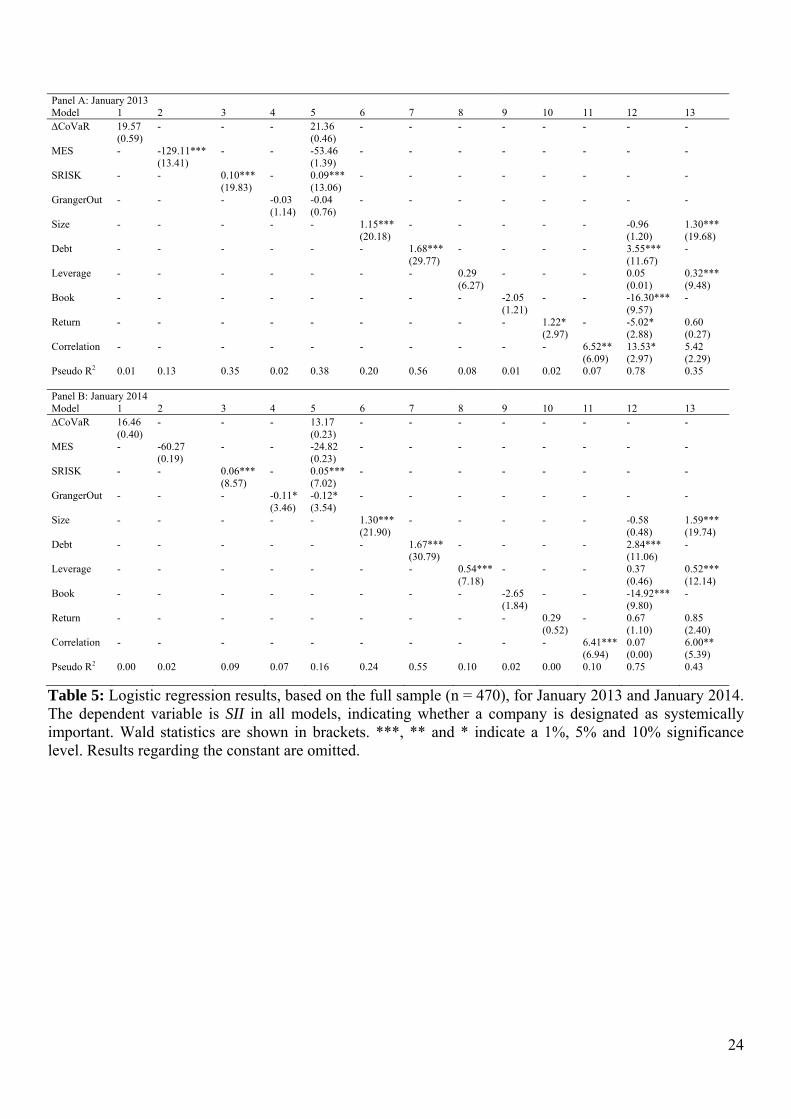
4.2. Results of the Second Approach (Classification as SII in 2013)

The second approach focuses on the information about which institutions have been labeled as

systemically important in 2013 by national and international regulators. It is evaluated if

sophisticated or simple systemic risk measures are more suitable to explain which institutions

are designated as contributing to systemic risk. The results regarding the variable SII are

presented in Table 5. Panel A illustrates the results for January 2013, and therefore, can be

considered the ex ante perspective. In contrast, Panel B illustrates the results for January 2014

and represents the ex post perspective. Models one to five show the results of the regressions

regarding the sophisticated systemic risk measures. Models six to thirteen illustrate the results

regarding the simple systemic risk measures.

It seems that sophisticated systemic risk measures have explanatory power to indicate which

institutions are deemed systemically important, ex ante (Panel A of Table 5). In particular, the

results for MES (model two) and SRISK (model three) are significant at a 1% level. The best

goodness of fit is achieved in model five, which includes all sophisticated risk measures. In

this model, only SRISK is significant at a 1% level. In comparison with the results of the first

approach in Table 3 (Panel A), the results at hand provide stronger evidence that systemic risk

measures might be able to detect institutions contributing to systemic risk.

Regarding the simple systemic risk measures (models six to thirteen), Size (model six), Debt

(model seven), Return (model ten) and Correlation (model eleven) are significant at least at a

10% level. The results for Size and Debt are robust in the way that these variables are

significant, even when controlling for other simple systemic risk measures (models twelve

and thirteen).

It is interesting that if Debt is included in the model, Size and Leverage are no longer

significant (model twelve). However, if Debt is not included, Size and Leverage are

significant (model thirteen). The pseudo R2 figures are high for Debt in model seven (0.56)

and in model twelve, which includes Debt and other simple measures (0.78). Models without

Debt have a pseudo R2 statistic at the most of 0.35 (model thirteen). This pattern suggests that

the total amount of debt is suitable for indicating ex ante institutions contributing to systemic

risk. In addition, Debt seems to be a better indicator than SRISK, since the pseudo R2 statistic

is higher (0.56 vs. 0.35). In general, the results seem to be in line with the results of the first

approach. In Table 3 (Panel A) and Table 5 (Panel A) Debt has the highest explanatory

power.

24

Panel A: January 2013 Model 1 2 3 4 5 6 7 8 9 10 11 12 13 CoVaR 19.57 - - - 21.36 - - - - - - - -

(0.59) (0.46) MES - -129.11*** - - -53.46 - - - - - - - -

(13.41) (1.39) SRISK - - 0.10*** - 0.09*** - - - - - - - -

(19.83) (13.06) GrangerOut - - - -0.03 -0.04 - - - - - - - -

(1.14) (0.76) Size - - - - - 1.15*** - - - - - -0.96 1.30***

(20.18) (1.20) (19.68) Debt - - - - - - 1.68*** - - - - 3.55*** -

(29.77) (11.67) Leverage - - - - - - - 0.29 - - - 0.05 0.32***

(6.27) (0.01) (9.48) Book - - - - - - - - -2.05 - - -16.30*** -

(1.21) (9.57) Return - - - - - - - - - 1.22* - -5.02* 0.60

(2.97) (2.88) (0.27) Correlation - - - - - - - - - - 6.52** 13.53* 5.42

(6.09) (2.97) (2.29) Pseudo R2 0.01 0.13 0.35 0.02 0.38 0.20 0.56 0.08 0.01 0.02 0.07 0.78 0.35 Panel B: January 2014 Model 1 2 3 4 5 6 7 8 9 10 11 12 13 CoVaR 16.46 - - - 13.17 - - - - - - - - (0.40) (0.23) MES - -60.27 - - -24.82 - - - - - - - - (0.19) (0.23) SRISK - - 0.06*** - 0.05*** - - - - - - - - (8.57) (7.02) GrangerOut - - - -0.11* -0.12* - - - - - - - - (3.46) (3.54) Size - - - - - 1.30*** - - - - - -0.58 1.59*** (21.90) (0.48) (19.74) Debt - - - - - - 1.67*** - - - - 2.84*** - (30.79) (11.06) Leverage - - - - - - - 0.54*** - - - 0.37 0.52*** (7.18) (0.46) (12.14) Book - - - - - - - - -2.65 - - -14.92*** - (1.84) (9.80) Return - - - - - - - - - 0.29 - 0.67 0.85 (0.52) (1.10) (2.40) Correlation - - - - - - - - - - 6.41*** 0.07 6.00** (6.94) (0.00) (5.39) Pseudo R2 0.00 0.02 0.09 0.07 0.16 0.24 0.55 0.10 0.02 0.00 0.10 0.75 0.43

Table 5: Logistic regression results, based on the full sample (n = 470), for January 2013 and January 2014. The dependent variable is SII in all models, indicating whether a company is designated as systemically important. Wald statistics are shown in brackets. ***, ** and * indicate a 1%, 5% and 10% significance level. Results regarding the constant are omitted.

25

Sophisticated systemic risk measures cannot explain, ex post, which companies are designated

to be systemically important, as illustrated in Panel B of Table 5. CoVaR and MES are not

significant in any model (model one, two and five). GrangerOut is significant at 5% and 10%

levels in models four and five, respectively, but the algebraic signs of the coefficients are

negative. This implies that the companies are systemically contributing to systemic risk,

which are deemed by Granger-Causality Networks not to be systemically relevant.

Lastly, SRISK is significant at a 1% level in models three and five. However, this cannot be

interpreted as evidence for the suitability of SRISK, since the pseudo R2 statistics of models

three and five are very low (0.09 and 0.16). These results are in contrast to the ones of the first

approach in Table 3 (Panel C), since, in the first approach, SRISK seems to be suitable for the

ex post perspective.

Considering the simple systemic risk measures in Panel C of Table 5, the results reveal that

Size (model six), Debt (model seven), Leverage (model eight) and Correlation (model ten) all

have significant explanatory power at a 1% level. However, taking several simple systemic

risk measures together into account leads to similar results, as presented in Panel A of Table

5.

In all models in which Debt is included, the variable is strongly significant and the pseudo R2

statistics are high (0.55 in model seven and 0.75 in model twelve). Models without Debt have

much lower pseudo R2 results and other variables are only significant in certain model

specifications. For example, Correlation is significant at a 1% and 5% level in models eleven

and thirteen, respectively, but not significant in model twelve. In contrast to the first approach

(Panel C of Table 3) where, ex post, sophisticated risk measures had comparable explanatory

power as simple systemic risk measures, the results at hand show that Debt has clearly the

most explanatory power.

26

I again perform a robustness test for a subsample of only financial services companies. Table

12 in the Appendix illustrates the results which are for January 2013 (Panel A) and January

2014 (Panel B). The subsample size is 82. This time, the results for the full sample are only

partially supported. For financial services companies, ex ante, sophisticated systemic risk

measures are found to have much more explanatory power. SRISK is significant at a 1% level

in all relevant models and the pseudo R2 statistics are high, with 0.56 (model three) and 0.61

(model five). Regarding the simple systemic risk measures, ex ante, a combined model of all

variables still has the highest pseudo R2 figure with 0.80 (model twelve), but, in this model,

no variable is significant.

For the ex post perspective in Panel B, the same pattern can be found. SRISK is significant at

a 1% level in models three and five. Furthermore, the pseudo R2 figures of these models are

rather high, with 0.30 and 0.43. In contrast, the variable Debt is only significant in model

seven at a 1% level, but the highest pseudo R2 figure is still achieved by a combined simple

systemic measures model with 0.82.

All in all, the results for the sophisticated systemic risk measures are much better for the

subsample, than in the case of the full sample. This is not astonishing, since the measures

have been developed mainly with the banking industry in mind, and therefore, are calibrated

to deliver the best results in the case of banks. Other industries were not considered in the

development, even though non-financial companies can also contribute to systemic risk.

27

4.3. Discussion

The results suggest that CoVaR is not able to correctly identify institutions which contribute

to systemic risk ex ante or ex post, neither at the moment, nor during the financial crisis.

Besides its popularity, this result could be expected, since major shortcomings of this

sophisticated risk measure are already pointed out in the literature. For example, Benoit et al.

(2013) illustrate that an institution’s CoVaR is proportional to its Value at Risk, and

therefore, an institution’s contribution to systemic risk is seen in isolation from the system. In

addition, Löffler and Raupach (2013) dispute the usefulness of CoVaR, since an increase of

an institution’s idiosyncratic risk decreases its contribution to systemic risk, according to the

risk measure.

For MES the results are nearly as poor as for CoVaR. Only from the ex ante perspective of

2013 does it seem to correctly identify institutions which contribute to systemic risk.

However, these results could be driven by the fact that some institutions have been already

labeled as systemically relevant in 2012, and therefore, their share prices dropped

substantially at the announcement date. My findings are in line with Idier et al. (2013, p. 18),

who analyze whether MES would have been suitable, in advance, to identify the banks

impaired the most by the financial crisis. According to their analysis, MES is not. They “thus

strongly doubt that the MES can really help regulators identify systematically important banks

on the eve of a future severe systemic crisis.”

According to Benoit et al. (2013), SRISK is a compromise of the too-big-to-fail and the too-

interconnected-to-fail paradigm. The “interconnectedness” is considered via MES and its

proportionality to its firm beta. At the same time, “size” is considered by the equity and debt

levels of a company. However, this promising approach is only partially supported by my

results. On the one hand, most of the time, SRISK can correctly identify the institutions which

contribute to systemic risk. Out of 32 models which include SRISK as an independent

variable, in 22 models, SRISK is significant and the models have at least a decent fit. On the

other hand, in six models, SRISK is not significant, and what is much more important, in two

models, it is misleading. In addition, the question remains if the results are mainly driven by

one of the constituents of SRISK – equity, debt and MES – or indeed are the outcome of the

composition.

The last sophisticated systemic risk measure I evaluate is the Granger-Causality Network. In

general, the key statement of Billio et al. (2012) is supported by my analyses: the overall

28

interconnectedness in the market is increasing during the financial crisis. In January 2007,

there are 10’911 (4.91% of all possible connections) Granger-causality connections between

the S&P 500 companies; in January 2008, there are 12’503 (5.62%); and in January 2009,

there are 22’225 (10.00%) connections. The results about whether the Granger-causality

relationships can successfully indicate the companies which contribute to systemic risk are

mixed. Out of the 32 models, GrangerOut is significant in twelve models; in 16, it is not

significant, and in four, it is misleading (significant, but with a negative algebraic sign).

The robustness tests show that the results are generally the same for financial services

institutions. Only in the case of the second approach, do the sophisticated systemic risk

measures fare better for the subsample (only financial services companies) than for the full

sample (all companies). Therefore, one cannot argue that the sophisticated risk measures are

suitable conditional on the limitation that they are only relevant for the context of financial

institutions.

Regarding the simple systemic risk measures, three results are worth discussing. First, the size

variables, Size and Debt, are most suitable for indicating companies contributing to systemic

risk. This could be expected, since the size of an institution is considered by regulators in

determining the contribution of an institution to systemic risk (see, for example, IAIS, 2013).

It is interesting that the market capitalization of a company is not the best indicator, but the

total debt level of a company is. One explanation could be that the severity of spillover effects

(i.e., interconnections in extreme conditions between institutions), are primarily driven by

counterparty credit risk and not by market risks (e.g., equity and interest rate risks). The

volatility of stock prices is even high in normal times.25 Therefore, extreme stock price

movements are expected by the market and the financial system is robust towards them. In

contrast, default rates are extremely low and the financial system never had to prove that it is

stable, even when debt cannot be paid on a large scale.26 This puts the results for SRISK into

perspective. As Benoit et al. (2013) suggest, SRISK is highly correlated to leverage and total

liabilities. The goodness of fit of the models, including Debt, always exceeds the SRISK

models. Consequently, the explanatory power of SRISK might be simply driven by debt.

However, total debt as reported in the balance sheets, as an indicator for systemic relevance,

does have some shortcomings. For example, all off-balance sheet exposures are not

considered.

25 E.g., between 1970 and 2005, the maximal loss within one week of the S&P 500 composite index was 22%. 26 E.g., according to Vazza and Kraemer (2013), the S&P investment-grade default rates between 1981 and

2012 never exceeded 0.42%.

29

Second, the results for the leverage variables (Leverage and Book) are very mixed. In models

without the variable Debt, Leverage often has explanatory power. However, in models

controlling for Debt, the explanatory power of Leverage is often not significant. Furthermore,

Book has a negative algebraic sign in all models in which the variable is significant. This

means that, on the one hand, leverage ratios are not very well suited to detect companies

contributing to systemic risk and, on the other hand, low leverage ratios can be an indicator of

systemic risk. These results are in sharp contrast to the majority view of regulators and

academics who emphasize that leverage ratios are at least a good indicator for companies

which are vulnerable to systemic risk (see, e.g., FSB, 2009; Baluch et al., 2011; Haldane,

2012; IAIS, 2013). An explanation for this result could be that the vulnerability and the

contribution to systemic risk are indeed two different concepts: an institution vulnerable to

systemic risk needs not necessarily contribute to it and vice versa. For example, a very small,

highly leveraged bank is intuitively not very robust towards adverse market situations.

However, the leverage itself is not a good indicator, in this case, for a contribution to systemic

risk, since the total debt level of the institution is small. Therefore, its impact on other

institutions, in the case of a bankruptcy, is very limited. Another argument which can explain

why the results for leverage variables are mixed is presented by Papanikolaou and Wolff

(2014). After the financial crisis of 2008 financial services institutions had to deleverage and

put asset prices under pressure. As a consequence the amount of available credit shrank and

systemic risk in the overall market went up. Therefore, according to the literature, it is

possible that not so much the leverage of institutions contributes to systemic risk but a sudden

deleveraging.

Third, comparing the fit of the models combining the sophisticated systemic risk measures

with models combining the simple measures illustrates that simple measures are more

powerful. Consequently, simple systemic risk measures can be regarded as more suitable to

detect companies contributing to systemic risk than sophisticated systemic risk measures. One

has to keep in mind, though, that this result is primarily due to Debt; other simple measures do

not fare much better as their sophisticated counterparts.

As mentioned in Section 1, two main assumptions are made. First, regulators successfully

supported the institutions contributing most to systemic risk during the financial crisis in

2008, as well as designated correctly the SIIs in 2013. Second, the contribution to the

systemic risk of a company is independent from the general state of the system. If the first

assumption is violated, the results of this paper would suggest that the wrong institutions have

30

been supported during the financial crisis, since the sophisticated risk measures and the

decisions of regulators are obviously not in line. Consequently, billions of USD could have

been wasted for institutions which did not need the financial support. The vice versa situation,

that some institutions needed financial support and received none, is unlikely, since the

financial system did not break down. If the second assumption is violated and the contribution

of an institution to systemic risk is dependent on the state of the system, the usefulness of all

current microprudential sophisticated risk measures has to be doubted, since none takes the

state of the system into account.

31

5. Conclusion

In this paper, I empirically evaluate whether sophisticated risk measures or simple systemic

risk measures are more suitable to detect institutions which contribute most to systemic risk. I

use two approaches, which use different variables approximating the systemic relevance of an

institution. In the first approach, I use information about which institutions received financial

support during the financial crisis and what amount they received. In the second approach, the

systemic relevance is approximated by the fact of whether or not an institution is currently

regarded as systemically important by national or international supervisors. Finally, I regress

the systemic relevance variables on the various sophisticated and simple systemic risk

measures.

The results of the paper suggest that simple systemic risk measures are more suitable to detect

institutions contributing to systemic risk than sophisticated ones. This finding holds true for

an ex ante and ex post perspective, regarding the point in time when the dependent and

independent variables are calculated. In addition, this finding is valid for a broad sample of

diverse companies (companies included in the S&P 500 composite index), as well as for a

sample only considering financial institutions (all S&P 500 composite index companies

labeled as banks, insurers, real estate or financial services companies).

In particular, the total amount of debt of a company is the strongest indicator for systemic

relevance, followed by its market capitalization. Interestingly, the results for the leverage

variables are rather mixed. Leverage seems not to have such a strong impact, as currently

assumed (see, e.g., FSB, 2009).

Among the sophisticated systemic risk measures, the best results are achieved for SRISK.

Most of the time, it can successfully indicate companies which received financial support

during the financial crisis and companies which are regarded currently as contributing to

systemic risk. However, in the case of explaining, ex ante, the amount of financial support

each institution received in 2008, it is misleading. This is a meaningful finding, since SRISK

combines market based information (via MES and market capitalization), as well as balance

sheet information (debt), and shows that combining sophisticated and simple systemic risk

measures might be a viable attempt to measure the systemic risk of institutions.

The results are of importance to academics and their choice of an adequate risk measure. Each

sophisticated measure should at least have more explanatory power than the total amount of

debt in determining companies contributing to systemic risk. Furthermore, the results can be

32

of use for regulators assessing if an indicator based approach to identify systemically

important institutions is sufficient or other measures should be considered as well. In my

opinion, the regulatory discussion should focus more on the robustness of the financial system

towards a systemic crisis, instead of focusing on institutions contributing to systemic risk.

Labeling institutions as systemically relevant might create the false impression that regulators

or academics are able to do so correctly, and therefore, might create a risk of its own.

Despite the vast number of studies on measuring systemic risk and the last financial crisis,

there is still a need for further research. Firstly, in this paper, the assumption is made that

during the financial crisis, financial support was given to the institutions which were

contributing most to systemic risk. This assumption is commonly made, but it has not been

evaluated yet whether it is true in all regards. More importantly, there is no discussion if the

billions of dollars for the bailout programs were spent effectively and whether the institutions

really needed the financial support for keeping the financial system stable. Secondly,

sophisticated risk measures currently under discussion, try to achieve additivity (i.e., the sum

of the systemic risk contributions of each company within a system equals the systemic risk of

the system). However, it is not clear whether feedback effects can be ruled out. Maybe the

state of the system influences the systemic risk contribution of an institution as well. Finally,

as illustrated in this paper, and by the discussion in the literature about systemic risk

measures, there is still no commonly acceptable measure, approach or framework which can

properly determine systemic risk.

33

References

Acharya, V.V., Pedersen, L.H., Philippon, T., Richardson, M., 2010. Measuring systemic risk.

Working Paper. New York University. Available at:

http://pages.stern.nyu.edu/~sternfin/vacharya/public_html/MeasuringSystemicRisk_final.

pdf (24th October 2014).

Acharya, V.V., Engle, R., Richardson, M., 2012. Capital shortfall: A new approach to ranking

and regulating systemic risks. American Economic Review: Papers & Proceedings

102(3): 59-64.

Adrian, T., Brunnermeier, M.K., 2011. CoVaR. Working Paper. Federal Reserve Bank of

New York. Available at: http://www.princeton.edu/~markus/research/papers/CoVaR.pdf

(24th October 2014).

Baluch, F., Mutenga, S., Parsons, C., 2011. Insurance, systemic risk and the financial crisis.

Geneva Papers on Risk and Insurance—Issues and Practice 36(1): 126-163.

Balla, E., Ergen, I., Migueis, M., 2014. Tail dependence and indicators of systemic risk for

large US depositories. Journal of Financial Stability 15: 195-209.

Benoit, S., Colletaz, G., Hurlin, C., Pérignon, C., 2013. A theoretical and empirical

comparison of systemic risk measures. Working Paper. University of Orléans. Available

at: http://papers.ssrn.com/sol3/papers.cfm?abstract_id=1973950 (30th October 2014).

Billio, M., Getmansky, M., Lo, A.W., Pelizzon, L., 2012. Econometric measures of

connectedness and systemic risk in the finance and insurance sectors. Journal of Financial

Economics 104, 535-559.

Bisias, D., Flood, M., Lo, A.W.,Valavanis, S., 2012. A survey of systemic risk analytics.

Working Paper. MIT Operations Research Center. Available at:

http://www.treasury.gov/initiatives/wsr/ofr/Documents/OFRwp0001_BisiasFloodLoVala

vanis_ASurveyOfSystemicRiskAnalytics.pdf (24th October 2014).

Brewer III, E., Jagtiani, J., (2013): How much did banks pay to become too-big-to-fail and to

become systemically important? Journal of Financial Services Research 43(1): 1-35.

Brownlees, C.T., Engle, R.F., 2012. Volatility, correlation and tails for systemic risk

measurement. Working Paper. Universitat Pompeu Fabra. Available at:

http://papers.ssrn.com/sol3/papers.cfm?abstract_id=1611229 (06th November 2014).

Calice, G., Ioannidis, C., Williams, J., (2012). Credit derivatives and the default risk of large

complex financial institutions. Journal of Financial Services Research 42(1/2): 85-107.

34

Chen, H., Cummins, J.D., Viswanathan, K.S., Weiss, M.A., 2014. Systemic risk and the

interconnectedness between banks and insurers: An econometric analysis. Journal of Risk

and Insurance 81(3): 623-652.

Congress of the U.S., 2008. Emergency Economic Stabilization Act. Available at:

http://www.house.gov/apps/list/press/financialsvcs_dem/essabill.pdf (24th October 2014).

Corvarsce, G., 2013. Measuring systemic risk: an international framework. Working Paper.

Available at: http://www.financialrisksforum.com/risk2013/work/8292433.pdf (24th

October 2014).

DeYoung, R., 2012. A commentary on “measuring systemic risk“. Journal of Financial

Services Research 42(1/2): 109-114.

Drehmann, M., Tarashev, N., 2011. Systemic importance: some simple indicators. BIS

Quarterly Review, March 2011. Available at:

http://www.bis.org/publ/qtrpdf/r_qt1103.htm (24th October 2014).

Duca, M.L, Peltonen, T.A., 2013. Assessing systemic risks and predicting systemic events.

Journal of Banking & Finance 37(7): 2183-2195.

Eling, M., Pankoke, D., 2014. Systemic risk in the insurance sector: Review and directions for

future research. Working Paper. University of St. Gallen.

Federal Deposit Insurance Corporation, 2008. Temporary Liquidity Guarantee Program; Final

Rule. Available at: https://www.fdic.gov/regulations/resources/TLGP/archive.html (24th

October 2014).

Federal Reserve System, 2008. Statement by Chairman Bernanke on Fannie Mae and Freddie

Mac. Press Release. Available at:

http://www.federalreserve.gov/newsevents/press/other/20080907a.htm (24th October

2014).

Federal Reserve System, 2014. Bear Stearns, JP Morgan Chase, and Maiden Lane LLC.

Available at: http://www.federalreserve.gov/newsevents/reform_bearstearns.htm (24th

October 2014).

FSOC (Financial Stability Oversight Council), 2013. Designations. Website. Available at:

http://www.treasury.gov/initiatives/fsoc/designations/Pages/default.aspx (27th October

2014).

FSB (Financial Stability Board), 2009. Report to G20 Finance Ministers and Governors.

Technical Report. Available at: http://www.bis.org/publ/othp07.htm (24th October 2014).

35

FSB (Financial Stability Board), 2012. Update of group of global systemically important

banks (G-SIBs). Technical Report. Available at:

http://www.financialstabilityboard.org/publications/r_121031ac.htm (24th October 2014).

FSB (Financial Stability Board), 2013a. Global systemically important insurers (G-SIIs) and

the policy measures that will apply to them. Technical Report. Available at:

http://www.financialstabilityboard.org/publications/r_130718.htm (24th October 2014).

FSB (Financial Stability Board), 2013b. 2013 update of group of global systemically

important banks (G-SIBs). Technical Report. Available at:

http://www.financialstabilityboard.org/publications/r_131111.htm (27th October 2014).

FTSE International Limited, 2012. ICB structure and definitions document. Technical Report.

Available at: http://www.icbenchmark.com/Site/ICB_Structure (29th October 2014).

Gorton, G.B., Metrick, A., 2012. Getting up to speed on the financial crisis: one-weekend-

reader’s guide. Working Paper. National Bureau of Economic Research. Available at:

http://www.nber.org/papers/w17778.pdf (24th October 2014).

Haldane, A.G., 2012. The dog and the frisbee. Speech. Bank of England. Available at:

http://www.bankofengland.co.uk/publications/Pages/speeches/2012/596.aspx (24th

October 2014).

Harrington, S.E., 2009. The financial crisis, systemic risk, and the future of insurance

regulation. Journal of Risk and Insurance 76(4): 785-819.

Huang, X., Zhou, H., Zhu, H., 2009. A framework for assessing the systemic risk of major

financial institutions. Journal of Banking & Finance 33(11): 2036-2049.

Huang, X., Zhou, H., Zhu, H., 2012. Systemic risk contributions. Journal of Financial

Services Research 42(1-2): 55-83.

IAIS, 2013. Global systemically important insurers: Initial assessment methodology.

Technical Report. Available at: http://www.iaisweb.org/Financial-Stability-

Macroprudential-Policy-Surveillance-988 (24th October 2014).

Idier, J., Lamé, G., Mésonnier, J., 2013. How useful is the marginal expected shortfall for the

measurement of systemic exposure? A practical assessment. Working Paper. European

Central Bank. Available at: http://www.ecb.europa.eu/pub/pdf/scpwps/ecbwp1546.pdf

(30th October 2013).

Isidore, C., 2013. JPMorgan sues FDIC over Washington Mutual. CNN Money Article.

Available at: http://money.cnn.com/2013/12/18/news/companies/jpmorgan-fdic-lawuit/

(24th October 2014).

36

Jobst, A.A., 2014. Systemic risk in the insurance sector: A review of current assessment

approaches. Geneva Papers on Risk and Insurance—Issues and Practice 39: 440-470.

Katz, I., 2013. Regulators vote to label AIG, GE Capital systemically important. Bloomberg

News. Available at: http://www.bloomberg.com/news/2013-07-09/regulators-vote-to-

label-aig-ge-capital-systemically-important.html (24th October 2014).

Löffler, G., Raupach, P., 2013. Robustness and informativeness of systemic risk measures.

Working Paper. Deutsche Bundesbank. Available at:

http://www.bundesbank.de/Redaktion/EN/Downloads/Publications/Discussion_Paper_1/

2013/2013_03_11_dkp_04.pdf (24th October 2014).

Neale, F.R., Drake, P.P., Schorno, P., Semann, E., 2012. Insurance and interconnectedness in

the financial services industry. Working Paper. UNC Charlotte. Available at:

http://www.aria.org/meetings/2012%20Meetings/1F-Interconnectedness%20.pdf (28th

October 2014).

Palank, J, 2013. Bankruptcy Lawyer: Letting Lehman fail was ‘tragic error’. Wall Street

Journal Article. Available at: http://blogs.wsj.com/bankruptcy/2013/09/13/bankruptcy-

lawyer-letting-lehman-fail-was-tragic-error/ (24th October 2014).

Papanikolaou, N.I., Wolff, C.C.P., 2014. The role of on- and off-balance-sheet leverage of

banks in the late 2000s crisis. Journal of Financial Stability 14: 3-22.

Patro., D.K., Qi, M., Sun, X., 2013. A simple indicator of systemic risk. Journal of Financial

Stability 9: 105-116.

Pottier, S.W., Sommer, D.W., 2002. The effectiveness of public and private sector summary

risk measures in predicting insurer insolvencies. Journal of Financial Services Research

21(1/2): 101-116.

Rodríguez-Moreno, M., Peña, J.I., 2013. Systemic risk measures: the simpler the better?

Journal of Banking & Finance 37(6): 1817-1831.

Vazza, D., Kraemer, N.W., 2013. 2012 annual global corporate default study and rating

transitions. Technical Report. Available at:

http://www.nact.org/resources/NACT_2012_Global_Corporate_Default.pdf (04th

November 2014)

Weiß, G.N.F., Mühlnickel, J., 2014. Why do some insurers become systemically relevant?

Journal of Financial Stability 13: 95-117.

37

Appendix

Panel B: January 2008 Model 1 2 3 4 5 6 7 8 9 10 11 12 13 CoVaR -39.49* - - - 13.29 - - - - - - - -

(3.80 (0.25) MES - -124.81*** - - -93.59*** - - - - - - - -

(47.02) (17.42) SRISK - - 0.09*** - 0.05*** - - - - - - - -

(24.82) (6.78) GrangerOut - - - 0.05 0.04*** - - - - - - - -

(28.57) (11.31) Size - - - - - 0.51*** - - - - - -1.44*** 0.81***

(13.51) (15.08) (24.64) Debt - - - - - - 1.26*** - - - - 2.63*** -

(54.29) (44.59) Leverage - - - - - - - 0.35*** - - - -0.72 0.25***

(14.66) (0.36) (8.55) Book - - - - - - - - 0.01 - - -12.06*** -

(0.00) (27.35) Return - - - - - - - - - -1.86*** - 0.61 -2.37**

(11.63) (0.76) (9.34) Correlation - - - - - - - - - - 2.11** 1.91 1.36

(4.76) (1.40) (1.48) Pseudo R2 0.02 0.26 0.22 0.13 0.38 0.06 0.46 0.14 0.00 0.06 0.02 0.67 0.28

Table 6: Logistic regression results, based on the full sample (n = 474) for January 2008. The dependent variable is Support in all of the models, indicating whether a company received financial support during the financial crisis. Wald statistics are shown in brackets. ***, ** and * indicate a 1%, 5% and 10% significance level. Results regarding the constants are omitted.

Panel B: January 2008 Model 1 2 3 4 5 6 7 8 9 10 11 12 13 CoVaR -0.33** - - - -0.33** - - - - - - - -

(-2.11) (-2.15) MES - 0.15 - - 0.36** - - - - - - - -

(0.93) (2.13) SRISK - - 0.03 - 0.13 - - - - - - - -

(0.17) (0.73) GrangerOut - - - 0.36** 0.31* - - - - - - - -

(2.33) (1.95) Size - - - - - 0.66*** - - - - - 0.81*** -

(5.20) (5.95) Debt - - - - - - 0.61*** - - - - - 0.68***

(4.54) (4.30) Leverage - - - - - - - 0.13 - - - 0.10 -0.22

(0.79) (0.67) (-1.27) Book - - - - - - - - 0.26 - - - -

(1.61) Return - - - - - - - - - -0.13 - -0.36** -0.11

(-0.77) (-2.53) (-0.69) Correlation - - - - - - - - - - 0.25 -0.12 0.03

(1.52) (-0.86) (0.20) Adjusted R2 0.09 0.00 -0.03 0.11 0.22 0.41 0.35 -0.01 0.04 -0.01 0.03 0.50 0.33

Table 7: Least square regression results for January 2008. The sample (n = 37) only includes institutions which received financial support. The dependent variable is Amount in all models, indicating the amount of support a certain company received during the financial crisis. T-statistics are shown in brackets. ***, ** and * indicate a 1%, 5% and 10% significance level. Results regarding the constants are omitted.

38

Panel A: January 2007 Model 1 2 3 4 5 6 7 8 9 10 11 12 13 CoVaR -0.54 - - - -31.52 - - - - - - - -

(1.36) (0.75) MES - 7.74 - - 19.19 - - - - - - - -

(0.03) (0.11) SRISK - - -0.02 - -0.01 - - - - - - - -

(1.01) (0.45) GrangerOut - - - 0.03 0.03 - - - - - - - -

(2.55) (2.35) Size - - - - - 0.85*** - - - - - -1.66** 0.83**

(8.46) (5.68) (6.03) Debt - - - - - - 0.68*** - - - - 2.06*** -

(15.54) (16.57) Leverage - - - - - - - 0.24 - - - -0.33 0.10

(2.33) (1.50) (0.42) Book - - - - - - - - -0.41 - - -6.33*** -

(0.15) (7.12) Return - - - - - - - - - 0.88 - 1.30 0.81

(0.66) (0.69) (0.48) Correlation - - - - - - - - - - -4.12*** -2.46 -4.47***

(7.13) (1.59) (6.87) Pseudo R2 0.01 0.00 0.02 0.05 0.07 0.15 0.33 0.05 0.00 0.01 0.13 0.59 0.27 Panel C: January 2009 Model 1 2 3 4 5 6 7 8 9 10 11 12 13 CoVaR -11.66 - - - -24.71 - - - - - - - - (0.28) (0.70) MES - -8.89 - - -5.51 - - - - - - - - (2.48) (0.31) SRISK - - 0.06*** - 0.06** - - - - - - - - (7.00) (5.01) GrangerOut - - - 0.00 0.00 - - - - - - - - (1.30) (0.34) Size - - - - - 0.43** - - - - - -0.62 1.48*** (4.92) (0.87) (12.24) Debt - - - - - - 1.01*** - - - - 2.77*** - (16.02) (12.90) Leverage - - - - - - - -0.00 - - - -0.01 -0.00 (0.37) (0.12) (0.36) Book - - - - - - - - -1.02 - - -10.47*** - (1.01) (7.91) Return - - - - - - - - - -0.78 - 0.02 -7.11*** (0.85) (0.00) (11.16) Correlation - - - - - - - - - - -2.64** -3.42 -7.71*** (6.40) (1.56) (10.03) Pseudo R2 0.01 0.04 0.29 0.02 0.31 0.09 0.47 0.01 0.02 0.01 0.11 0.80 0.48

Table 8: Logistic regression results, based on the subsample (n = 84) of financial services companies for January 2007 and January 2009. The dependent variable is Support in all models, indicating whether a company received financial support during the financial crisis. Wald statistics are shown in brackets. ***, ** and * indicate a 1%, 5% and 10% significance level. Results regarding the constants are omitted.

39

Panel A: January 2007 Model 1 2 3 4 5 6 7 8 9 10 11 12 13 CoVaR -0.36** - - - -0.19 - - - - - - - -

(-2.26) (-1.50) MES - -0.23 - - -0.44*** - - - - - - - -

(-1.37) (-3.27) SRISK - - -0.62*** - -0.84*** - - - - - - - -

(-4.62) (-7.44) GrangerOut - - - -0.01 -0.08 - - - - - - - -

(-0.03) (-0.80) Size - - - - - 0.70*** - - - - - 0.70*** -

(5.63) (5.32) Debt - - - - - - 0.62*** - - - - - 0.82***

(4.58) (4.64) Leverage - - - - - - - 0.21 - - - 0.06 -0.30

(1.25) (0.45) (-1.68) Book - - - - - - - - 0.23 - - - -

(1.36) Return - - - - - - - - - -0.07 - -0.12 -0.05

(-0.43) (-0.94) (-0.35) Correlation - - - - - - - - - - -0.01 -0.12 -0.03

(-0.03) (-0.89) (-0.19) Adjusted R2 0.11 0.02 0.37 -0.03 0.65 0.47 0.36 0.02 0.02 -0.02 -0.03 0.44 0.37 Panel C: January 2009 Model 1 2 3 4 5 6 7 8 9 10 11 12 13 CoVaR -0.10 - - - -0.14 - - - - - - - - (-0.57) (-1.39) MES - -0.31* - - -0.14 - - - - - - - - (-1.87) (-1.35) SRISK - - 0.76*** - 0.71*** - - - - - - - - (6.49) (7.00) GrangerOut - - - 0.39** 0.34*** - - - - - - - - (2.43) (3.36) Size - - - - - 0.30* - - - - - 0.73*** - (1.80) (4.95) Debt - - - - - - 0.66*** - - - - - 0.70*** (4.85) (4.82) Leverage - - - - - - - 0.52*** - - - 0.49*** 0.09 (3.33) (3.69) (0.59) Book - - - - - - - - 0.21 - - - - (1.19) Return - - - - - - - - - -0.36** - -0.55*** -0.43** (-2.27) (-3.36) (2.72) Correlation - - - - - - - - - - 0.23 -0.33** -0.22 (1.38) (2.20) (-1.56) Adjusted R2 -0.02 0.07 0.56 0.12 0.69 0.06 0.42 0.25 0.13 0.11 0.03 0.57 0.57

Table 9: Least square regression results, based on a subsample (n = 35) of financial services companies for January 2007 and January 2009. The sample only includes institutions which received financial support. The dependent variable is Amount in all models, indicating the amount of support a certain company received during the financial crisis. T-statistics are shown in brackets. ***, ** and * indicate a 1%, 5% and 10% significance level. Results regarding the constants are omitted.

40

Panel B: January 2008 Model 1 2 3 4 5 6 7 8 9 10 11 12 13 CoVaR -5.18 - - - 23.08 - - - - - - - -

(0.03) (0.32) MES - -25.67 - - 35.59 - - - - - - - -

(1.61) (1.22) SRISK - - 0.04** - 0.05** - - - - - - - -

(5.87) (4.48) GrangerOut - - - 0.06*** 0.06*** - - - - - - - -

(12.22) (9.77) Size - - - - - 0.68*** - - - - - -1.01 1.18***

(7.29) (2.43) (11.34) Debt - - - - - - 0.65*** - - - - 1.67*** -

(15.40) (14.38) Leverage - - - - - - - 0.04 - - - -0.19* -0.00

(0.53) (2.82) (0.00) Book - - - - - - - - -0.53 - - -3.64* -

(0.26) (3.06) Return - - - - - - - - - -0.36 - 2.00 -2.64**

(0.27) (1.17) (5.27) Correlation - - - - - - - - - - -2.61* -3.46 -4.96**

(2.91) (1.85) (5.96) Pseudo R2 0.00 0.03 0.14 0.23 0.33 0.13 0.33 0.01 0.00 0.00 0.05 0.55 0.28

Table 10: Logistic regression results, based on a subsample (n = 84) of financial services companies for January 2008. The dependent variable is Support in all models, indicating whether a company received financial support during the financial crisis. Wald statistics are shown in brackets. ***, ** and * indicate a 1%, 5% and 10% significance level. Results regarding the constants are omitted.

Panel B: January 2008 Model 1 2 3 4 5 6 7 8 9 10 11 12 13 CoVaR -0.25 - - - -0.02 - - - - - - - -

(1.52) (-0.14) MES - 0.07 - - 0.27* - - - - - - - -

(0.40) (1.86) SRISK - - 0.51*** - 0.50*** - - - - - - - -

(3.39) (3.27) GrangerOut - - - 0.46*** 0.35** - - - - - - - -

(3.02) (2.50) Size - - - - - 0.62*** - - - - - 0.79*** -

(4.58) (5.24) Debt - - - - - - 0.58*** - - - - - 0.63***

(4.05) (3.69) Leverage - - - - - - - 0.16 - - - 0.10 -0.20

(0.91) (0.64) (-1.07) Book - - - - - - - - 0.20 - - - -

(1.14) Return - - - - - - - - - -0.15 - -0.41** -0.10

(-0.85) (-2.45) (-0.56) Correlation - - - - - - - - - - 0.27 -0.17 0.05

(1.61) (-1.02) (0.25) Adjusted R2 0.04 -0.03 0.24 0.19 0.38 0.36 0.31 -0.01 0.01 -0.01 0.04 0.45 0.27

Table 11: Least square regression results, based on a subsample (n = 35) of financial services companies for January 2008. The sample only includes institutions which received financial support. The dependent variable is Amount in all models, indicating the amount of support a certain company received during the financial crisis. T-statistics are shown in brackets. ***, ** and * indicate a 1%, 5% and 10% significance level. Results regarding the constants are omitted.

41

Panel A: January 2013 Model 1 2 3 4 5 6 7 8 9 10 11 12 13 CoVaR 5.72 - - - 45.01 - - - - - - - -

(0.05) (0.83) MES - -148.38*** - - 51.60 - - - - - - - -

(9.17) (0.31) SRISK - - 0.12*** - 0.14** - - - - - - - -

(10.20) (6.41) GrangerOut - - - -0.09 -0.08 - - - - - - - -

(2.29) (0.77) Size - - - - - 1.94*** - - - - - 1.32 2.45***

(14.16) (0.56) (11.31) Debt - - - - - - 1.17*** - - - - 1.70 -

(15.52) (2.10) Leverage - - - - - - - 0.12 - - - 1.17 0.19*

(1.91) (1.49) (3.21) Book - - - - - - - - -1.87 - - -33.77 -

(1.24) (2.38) Return - - - - - - - - - 1.37 - -5.64 -3.79

(1.03) (1.95) (2.32) Correlation - - - - - - - - - - 6.22* 14.42 4.81

(3.32) (2.03) (1.61) Pseudo R2 0.00 0.21 0.56 0.14 0.61 0.45 0.51 0.04 0.03 0.02 0.08 0.80 0.53 Panel B: January 2014 Model 1 2 3 4 5 6 7 8 9 10 11 12 13 CoVaR 5.48 - - - 3.56 - - - - - - - - (0.04) (0.01) MES - -77.24 - - 19.99 - - - - - - - - (1.48) (0.03) SRISK - - 0.08*** - 0.07*** - - - - - - - - (10.75) (6.77)

GrangerOut - - - -0.15** -0.15* - - - - - - - -

(5.19) (3.45) Size - - - - - 2.10*** - - - - - 2.09 2.12*** (15.21) (1.42) (14.56) Debt - - - - - - 1.19*** - - - - 1.732 - (15.66) (2.11) Leverage - - - - - - - 0.22 - - - 5.48** 0.26 (2.37) (3.88) (2.43)

Book - - - - - - - - -1.92 - - -84.02** -

(1.23) (4.21) Return - - - - - - - - - 0.95 - -1.07 1.53 (0.93) (0.15) (1.14) Correlation - - - - - - - - - - 1.50 -11.23 0.86 (0.49) (1.64) (0.12) Pseudo R2 0.00 0.03 0.30 0.23 0.43 0.50 0.51 0.05 0.03 0.02 0.01 0.82 0.54

Table 12: Logistic regression results, based on a subsample (n = 82) of financial services companies for January 2013. The dependent variable is SII in all models, indicating whether a company is designated as systemically important. Wald statistics are shown in brackets. ***, ** and * indicate a 1%, 5% and 10% significance level. Results regarding the constants are omitted.

42

Dependent Variable: Support Amount SII Model 1 2 3 4 5 6 7 8 9 10 11 12 13 14 15 16 Date 2007 2008 2009 2007 2008 2009 2007 2008 2009 2007 2008 2009 2013 2014 2013 2014 Panel A: CoVaR5% -211.98*** -206.85*** -78.75** - - - -0.21 -0.21 -0.24 - - - 23.63 12.00 - -

(25.30) (22.35) (4.69) (-1.26) (-1.27) (-1.45) (0.21) (0.05) CoVaR10% - - - -448.78*** -467.40*** -227.90*** - - - -0.16 -0.22 -0.26 - - 12.29 23.77

(37.05) (33.89) (11.35) (-0.99) (-1.34) (-1.61) (0.03) -0.09 Pseudo R2 0.13 0.12 0.02 0.22 0.20 0.06 - - - - - - 0.00 0.00 0.00 0.00 Adjusted R2 - - - - - - 0.02 0.02 0.03 0.00 0.02 0.04 - - - - Sample Size 472 471 472 472 471 472 37 36 37 37 36 37 470 470 470 470 Panel B: MES1% -21.96 -110.06*** -24.39*** - - - -0.16 0.04 0.04 - - - -81.74*** 5.00 - -

(1.56) (46.01) (43.48) (-0.96) (0.24) (0.26) (14.40) (0.03) MES10% - - - 28.99 -133.07*** -46.83*** - - - -0.04 0.07 -0.28* - - -177.49*** -129.33**

(1.03) (32.56) (42.74) (-0.21) (0.44) (-1.73) (14.44) (4.54) Pseudo R2 0.01 0.28 0.27 0.01 0.17 0.22 - - - - - - 0.14 0.00 0.14 0.04 Adjusted R2 - - - - - - 0.00 -0.03 -0.03 -0.03 -0.02 0.05 - - - - Sample Size 472 472 472 472 472 472 37 37 37 37 37 37 470 470 470 470 Panel C: SRISK1% 0.01 0.11*** 0.55*** - - - -0.51*** 0.16 0.70*** - - - 0.12*** 0.08*** - -

(1.20) (26.72) (43.56) (-3.57) (0.95) (5.63) -0.62*** (20.27) (18.14) SRISK10% - - 0.00 0.07*** 0.58*** - - - (-4.76) -0.05 0.69*** - 0.09*** 0.04***

(0.02) (22.00) (39.22) (-0.29) (5.48) (19.85) (3.31) Pseudo R2 0.01 0.27 0.68 0.00 0.16 0.65 - - - - - - 0.45 0.18 0.31 0.05 Adjusted R2 - - - - - - 0.24 0.00 0.47 0.37 -0.03 0.46 - - - Sample Size 472 472 472 472 472 472 37 36 34 37 36 34 470 470 470 470 Panel D: GrangerOut1% 0.06* 0.12*** 0.02*** - - - 0.14 0.33** 0.45*** - - - -0.18 -0.51* - -

(3.46) (23.58) (17.05) (0.85) (2.06) (3.01) (1.21) (3.65) GrangerOut10% - - - 0.01* 0.04*** 0.01*** - - 0.01 0.34** 0.33** - -0.02 -0.06*

(3.35) (29.60) (15.86) (0.08) (2.14) (2.07) (1.52) (3.76) Pseudo R2 0.01 0.10 0.08 0.01 0.13 0.07 - - - - - - 0.02 0.07 0.03 0.07 Adjusted R2 - - - - - - -0.01 0.08 0.18 -0.03 0.09 0.08 - - - - Sample Size 472 472 472 472 472 472 37 37 37 37 37 37 470 470 470 470

Table 13: Robustness tests for sophisticated systemic risk measures (partial models). Panel A refers to CoVaR whereas CoVaR5% takes into account the 5% quantil and CoVaR10% the 10% quantil. Panel B refers to the Marginal Expected Shortfall whereas MES1% and MES10% focus on the 1% respectively 10% days with the most negative stock market returns within the last year. Panel C refers to SRISK using MES1% and MES10%. Finally, Panel D shows the results for GrangerOut. GrangerOut1% and GrangerOut10% consider Granger-causality relationships at a significance level of 1% and 10%. In the cases of the dependent variables Support and SII, logistic regression models are used. Models regarding the dependent variable Amount employ least square regressions. Wald statistics are shown in brackets for models one to six and thirteen to sixteen. In models seven to twelve t-statistics are displayed instead. ***, ** and * indicate a 1%, 5% and 10% significance level. Results regarding the constants are omitted.

43

Dependent Variable: Support Amount SII Model 1 2 3 4 5 6 7 8 9 10 11 12 13 14 15 16 Date 2007 2008 2009 2007 2008 2009 2007 2008 2009 2007 2008 2009 2013 2014 2013 2014 CoVaR5% -226.62*** -105.53** -17.96 - - - -0.15 -0.21 -0.28*** - - - 74.70 30.55 - -

(25.79) (4.04) (0.09) (-1.04) (-1.24) (-2.82) (1.31) (0.25) CoVaR10% - - - -523.36*** -367.02*** -206.41* - - - -0.02 -0.19 -0.25** - - 52.36 65.48

(41.28) (16.62) (3.54) (-0.14) (-1.14) (-2.12) (0.32) (0.65) MES1% 10.18 -67.57*** 2.52 - - - -0.22 0.13 0.12 - - - -17.95 23.99 - -

(0.26) (14.88) (0.17) (-1.53) (0.72) (1.25) (0.31) (0.59) MES10% - - - 124.60*** -59.94** 13.36 - - - -0.23 0.15 -0.03 - - -91.23 -116.99*

(8.98) (4.50) (1.33) (-1.61) (0.77) (-0.25) (2.47) (3.19) SRISK1% 0.01 0.06*** 0.57*** - - - -0.50*** 0.13 0.64*** - - - 0.11*** 0.08*** - -

(0.45) (9.24) (28.99) (-3.45) (0.72) (6.61) (15.55) (14.25) SRISK10% - - - 0.00 0.04** 0.62*** - - - -0.69*** -0.06 0.65*** - - 0.07*** 0.03

(0.19) (5.61) (34.72) (-4.91) (-0.33) (5.43) (11.96) (1.86) GrangerOut1% 0.09** 0.09*** 0.02** - - - 0.17 0.25 0.43*** - - - -0.12 -0.39 - -

(6.19) (9.53) (6.36) 0.03*** (1.17) (1.39) (4.36) (0.38) (2.25) GrangerOut10% - - 0.02* (18.72) 0.01 - - - 0.00 0.32* 0.32*** - - -0.02 -0.07**

(2.91) (2.61) (-0.02) (1.81) (2.77) (1.16) (4.50) Pseudo R2 0.16 0.42 0.70 0.27 0.38 0.68 - - - - - - 0.47 0.23 0.35 0.15 Adjusted R2 - - - - - - 0.26 0.05 0.68 0.37 0.07 0.57 - - - - Sample Size 472 471 472 472 471 472 37 35 34 37 35 34 470 470 470 470

Table 14: Robustness tests for sophisticated systemic risk measures (full models). CoVaR5% takes into account the 5% quantil and CoVaR10% the 10% quantil. MES1% and MES10% focus on the 1% respectively 10% days with the most negative stock market returns within the last year. SRISK1% and SRISK10% indicate that for the calculation of SRISK, MES1% and MES10% are used. GrangerOut1% and GrangerOut10% consider granger-causality relationships at a significance level of 1% and 10%. In the cases of the dependent variables Support and SII, logistic regression models are used. Models regarding the dependent variable Amount employ least square regressions. Wald statistics are shown in brackets for models one to six and thirteen to sixteen. In models seven to twelve t-statistics are displayed instead. ***, ** and * indicate a 1%, 5% and 10% significance level. Results regarding the constants are omitted.