some thoughts on regularization for vector- valued inverse problems eric miller dept. of ece...
TRANSCRIPT
Some thoughts on regularization for vector-valued inverse problems
Eric Miller
Dept. of ECE
Northeastern University
Outline• Caveats• Motivating examples
– Sensor fusion: multiple sensors, multiple objects– Sensor diffusion: single modality, multiple objects
• Problem formulation• Regularization ideas
– Markov-random fields – Mutual information– Gradient correlation
• Examples• Conclusions
Caveats
• My objective here is to examine some initial ideas regarding multi-parameter inverse problems
• Models will be kept simple– Linear and 2D
• Consider two unknowns. – Case of 3 or more can wait
• Regularization parameters chosen by hand.• Results numerical. • Whatever theory there may be can wait for later
Motivating Applications
• Sensor fusion– Multiple modalities each looking at the
same region of interest– Each modality sensitive to a different
physical property of the medium
• Sensor diffusion– Single modality influenced by multiple
physical properties of the medium
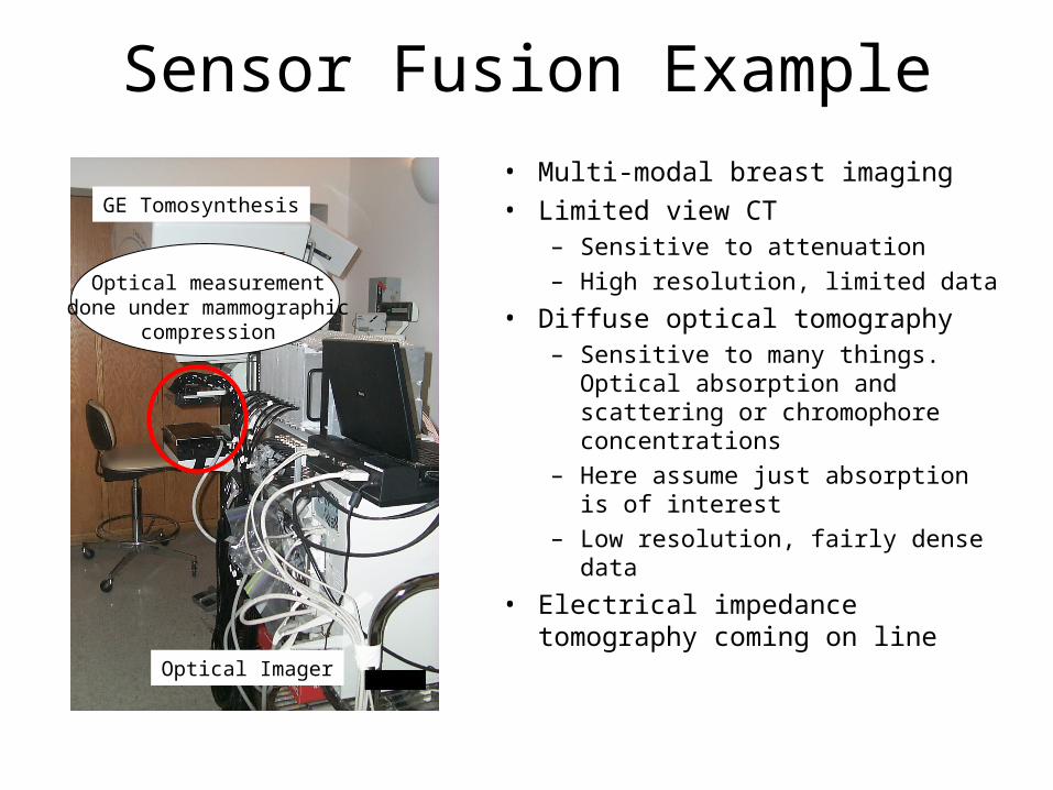
Sensor Fusion Example
• Multi-modal breast imaging• Limited view CT
– Sensitive to attenuation
– High resolution, limited data
• Diffuse optical tomography– Sensitive to many things. Optical
absorption and scattering or chromophore concentrations
– Here assume just absorption is of interest
– Low resolution, fairly dense data
• Electrical impedance tomography coming on line
GE Tomosynthesis
Optical Imager
Optical measurementdone under mammographic
compression
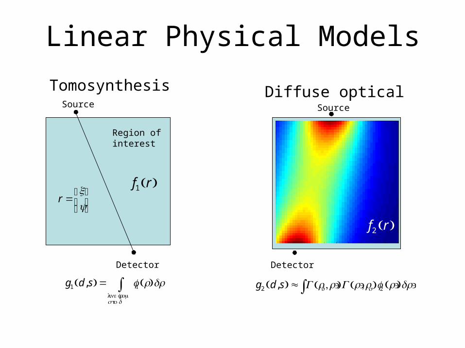
Linear Physical Models
TomosynthesisSource
Detector
Region of interest
g1 d, s( ) = f1 r( )drline froms to d
∫
Diffuse opticalSource
Detector
g2 d, s( ) ≈ G rd,r '( )G r',rs( )∫ f2 r '( )dr'
r =xy⎡
⎣⎢
⎤
⎦⎥
f1 r( )
f2 r( )
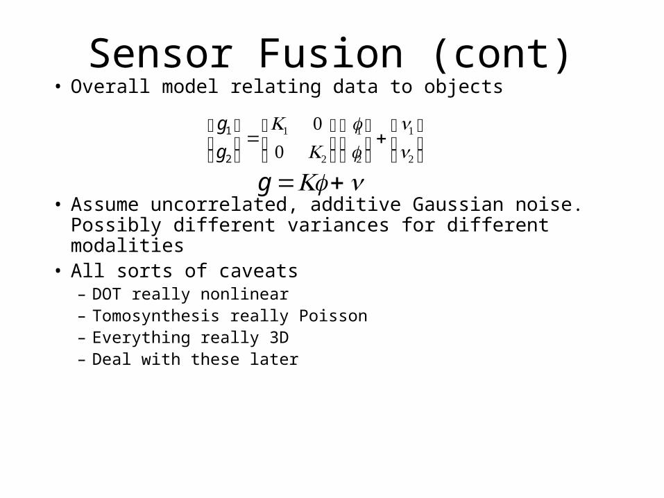
Sensor Fusion (cont)• Overall model relating data to objects
• Assume uncorrelated, additive Gaussian noise. Possibly different variances for different modalities
• All sorts of caveats– DOT really nonlinear– Tomosynthesis really Poisson– Everything really 3D– Deal with these later
g1
g2
⎡
⎣⎢
⎤
⎦⎥=
K1 00 K2
⎡
⎣⎢
⎤
⎦⎥
f1f2
⎡
⎣⎢
⎤
⎦⎥+
n1n2
⎡
⎣⎢
⎤
⎦⎥
g =Kf +n

De-Mosaicing
• Color cameras sub-sample red, green and blue on different pixels in the image
• Issues: filling in all of the pixels with all three colors
Bayer patternyredygreenyblue
⎡
⎣
⎢⎢⎢
⎤
⎦
⎥⎥⎥=
Kred 0 00 Kgreen 00 0 Kblue
⎡
⎣
⎢⎢⎢
⎤
⎦
⎥⎥⎥
fredfgreenfblue
⎡
⎣
⎢⎢⎢
⎤
⎦
⎥⎥⎥
• yred = observed red pixels over sub-sampled grid. 9 vector for example
• frwd = red pixels values over all pixels in image. 30 vector in example
• Kred = selection matrix with a single “1” in each row, all others 0. 9x30 matrix for example
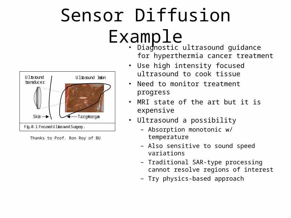
Sensor Diffusion Example• Diagnostic ultrasound guidance for
hyperthermia cancer treatment• Use high intensity focused ultrasound
to cook tissue• Need to monitor treatment progress• MRI state of the art but it is expensive• Ultrasound a possibility
– Absorption monotonic w/ temperature
– Also sensitive to sound speed variations
– Traditional SAR-type processing cannot resolve regions of interest
– Try physics-based approach
Skin
Fig. 0.1. Focused Ultrasound Surgery.
Ultrasound lesionUltrasoundtransducer
Target organ
Thanks to Prof. Ron Roy of BU

Ultrasound model• As with diffuse optical, exact model is based
on Helmholtz-type equation and is non-linear• Here we use a Born approximation even in
practice because problem size quite large (10’s of wavelengths on a side)
• Modelg rd ,rs ,ω( ) = α ω( )G rd,r ',ω( )G r',rs,ω( ) f1 r '( )dr'∫
+ β ω( )G rd,r ',ω( )G r',rs,ω( ) f2 r '( )dr'∫+noise
• f1 = sound speed• f2 = absorptionαβ = frequency dependent
“filters” for each parameter
g = K1 K2[ ]f1f2
⎡
⎣⎢
⎤
⎦⎥+n
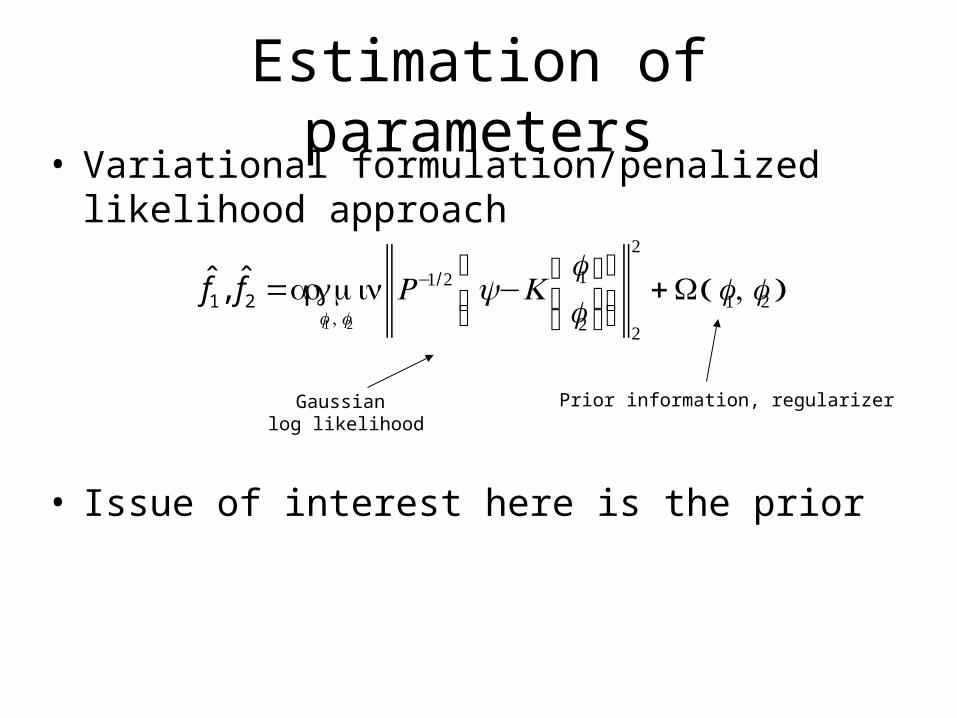
Estimation of parameters• Variational formulation/penalized likelihood
approach
• Issue of interest here is the prior
f̂1, f̂2 =argminf1 , f2
R−1/2 y−Kf1f2
⎡
⎣⎢
⎤
⎦⎥
⎛
⎝⎜⎞
⎠⎟2
2
+Ω f1, f2( )
Gaussian log likelihood
Prior information, regularizer
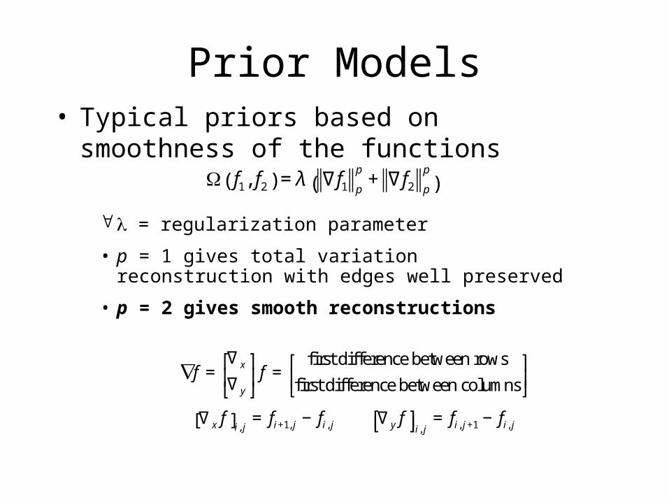
Prior Models• Typical priors based on smoothness of the
functionsΩ f1, f2( ) = λ ∇f1 p
p+ ∇f2 p
p
( )
= regularization parameter
• p = 1 gives total variation reconstruction with edges well preserved
• p = 2 gives smooth reconstructions
∇f =∇ x
∇ y
⎡
⎣⎢
⎤
⎦⎥ f =
first difference between rows
first difference between columns
⎡
⎣⎢
⎤
⎦⎥
∇ x f[ ]i, j = fi+1, j − fi, j ∇ y f⎡⎣ ⎤⎦i, j = fi, j+1 − fi, j
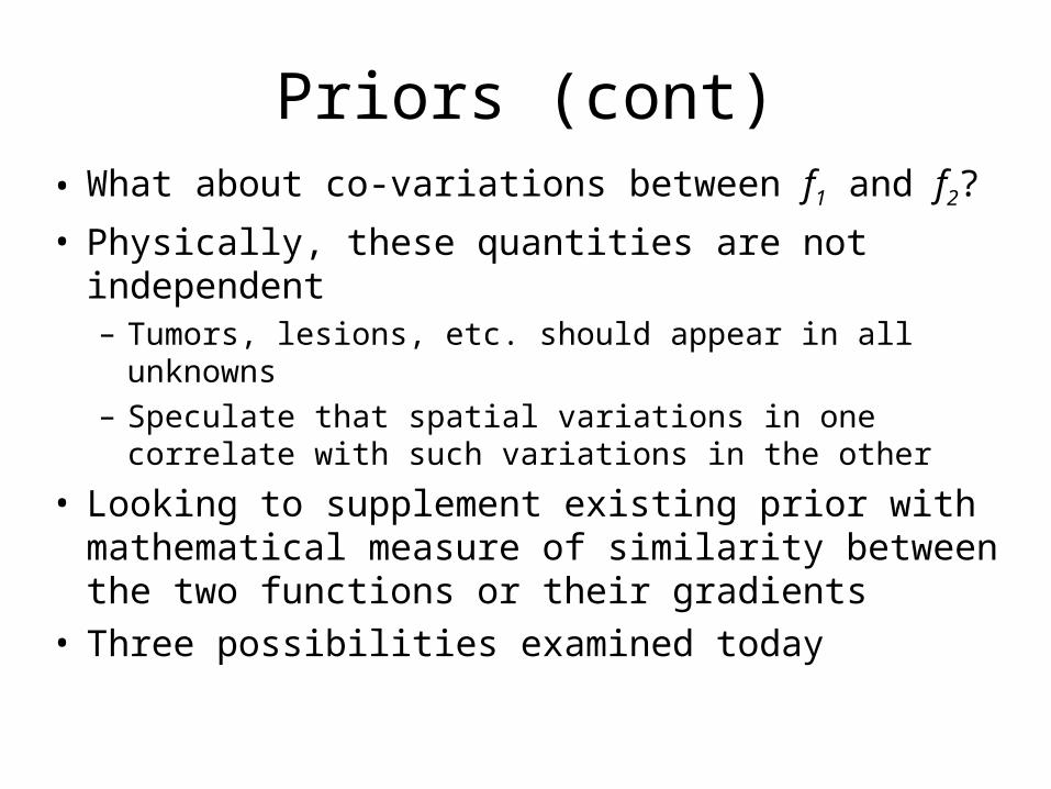
Priors (cont)• What about co-variations between f1 and f2?
• Physically, these quantities are not independent– Tumors, lesions, etc. should appear in all unknowns– Speculate that spatial variations in one correlate with
such variations in the other
• Looking to supplement existing prior with mathematical measure of similarity between the two functions or their gradients
• Three possibilities examined today
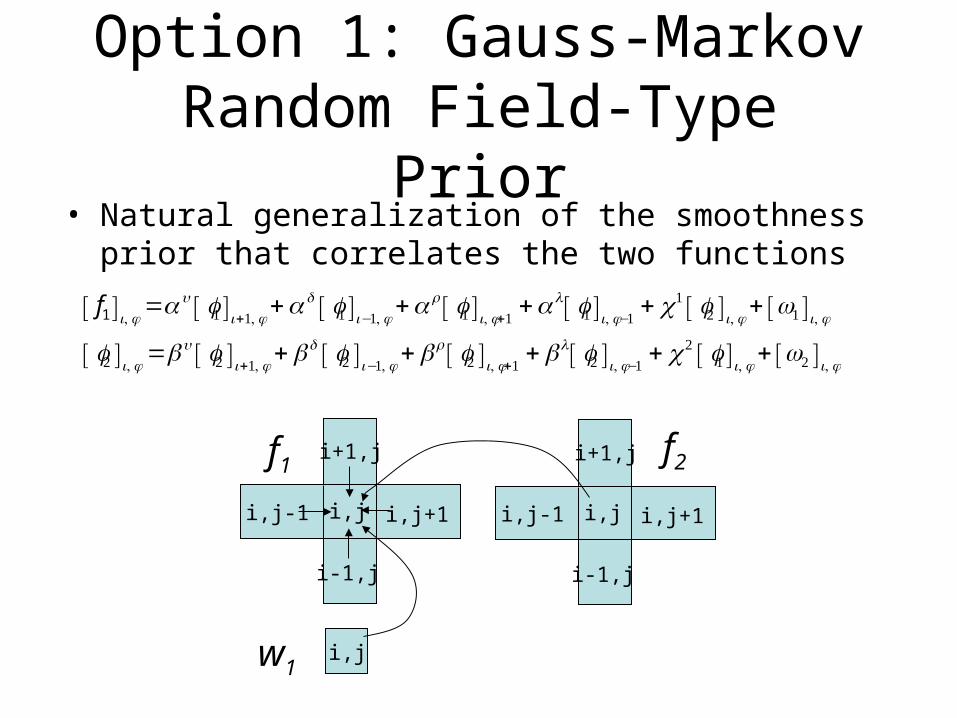
Option 1: Gauss-Markov Random Field-Type Prior
• Natural generalization of the smoothness prior that correlates the two functions
f1[ ]i, j =αu f1[ ]i+1, j +α
d f1[ ]i−1, j +αr f1[ ]i, j+1 +α
l f1[ ]i, j−1 + χ1 f2[ ]i, j + w1[ ]i, jf2[ ]i, j =βu f2[ ]i+1, j + βd f2[ ]i−1, j + β r f2[ ]i, j+1 + β l f2[ ]i, j−1 + χ 2 f1[ ]i, j + w2[ ]i, j
i,j
i+1,j
i-1,j
i,j+1i,j-1 i,j
i+1,j
i-1,j
i,j+1i,j-1
f1f2
i,jw1
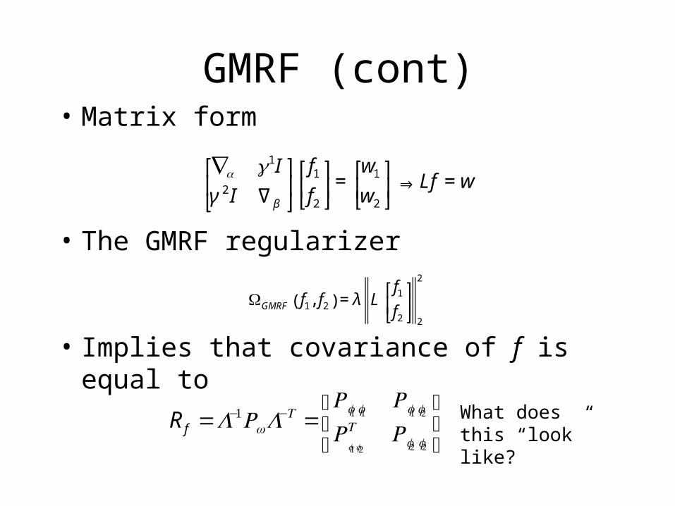
GMRF (cont)• Matrix form
• The GMRF regularizer
• Implies that covariance of f is equal to
∇α γ1I
γ 2I ∇β
⎡
⎣⎢
⎤
⎦⎥f1f2
⎡
⎣⎢
⎤
⎦⎥=
w1
w2
⎡
⎣⎢
⎤
⎦⎥⇒ Lf = w
R f =L−1RwL−T =
Rf1 f1Rf1 f2
Rf1 f2
T Rf2 f2
⎡
⎣⎢
⎤
⎦⎥ What does this
“look” like?
ΩGMRF f1, f2( ) = λ Lf1f2
⎡
⎣⎢
⎤
⎦⎥
2
2
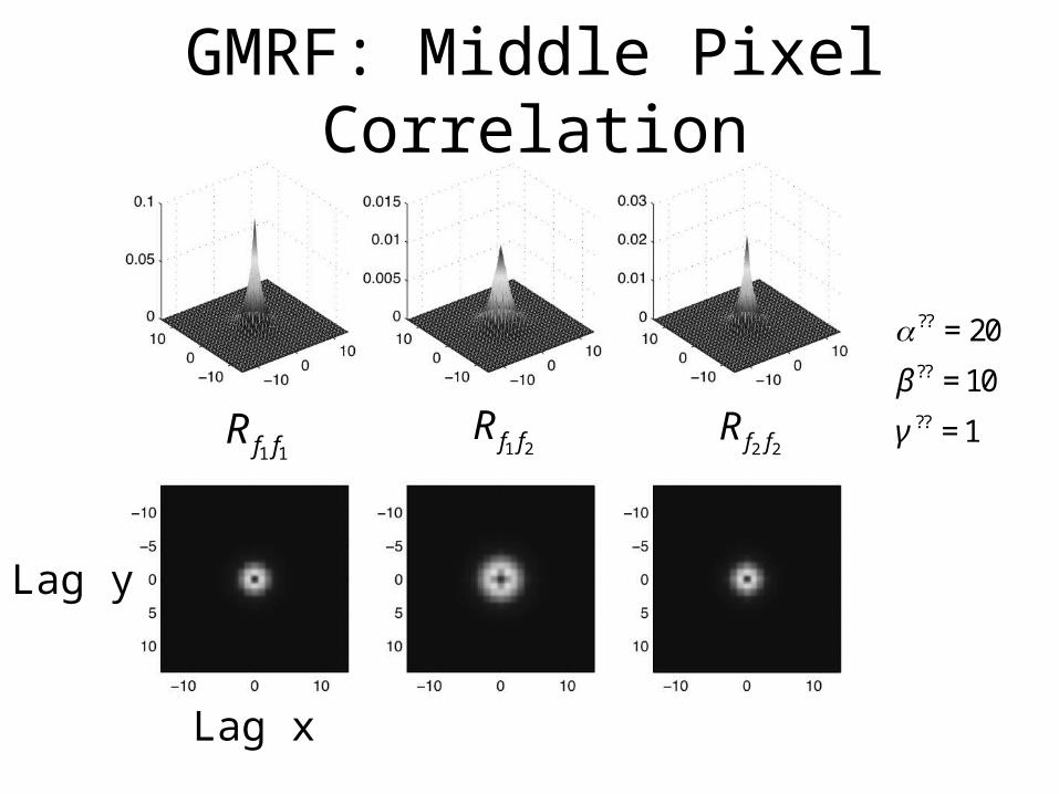
GMRF: Middle Pixel Correlation
Lag x
Lag y
R f1 f1 R f1 f2 R f2 f2
α ?? = 20
β ?? = 10
γ ?? = 1
GMRF: Comments
• Motivated by / similar to use of such models in hyperspectral processing
• Lots of things one could do– One line parameter estimation– Appropriate neighborhood structures– Generalized GMRF a la Bouman and
Sauer– More than two functions
Option 2: Mutual Information• An information theoretic measure of
similarity between distributions
• Great success as a cost function for image registration (Viola and Wells)
• Try a variant of it here to express similarity between f1 and f2
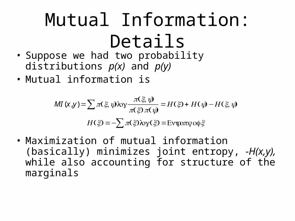
Mutual Information: Details• Suppose we had two probability distributions p(x)
and p(y)• Mutual information is
• Maximization of mutual information (basically) minimizes joint entropy, -H(x,y), while also accounting for structure of the marginals
MI(x, y) = p x,y( )logp x,y( )
p x( )p y( )=H x( ) + H y( )−H x,y( )∑
H x( ) =− p x( )∑ log x( ) =Entropy of x

Mutual Information: Details• Mutual information registration used not the images
but their histograms• Estimate histograms using simple kernel density
methods
and similarly for p(y) and p(x,y)
p x( ) =1N
K x− f1[ ]i( )i=1
N
∑
K x( ) =1
2πσ 2e−
x2
2σ 2
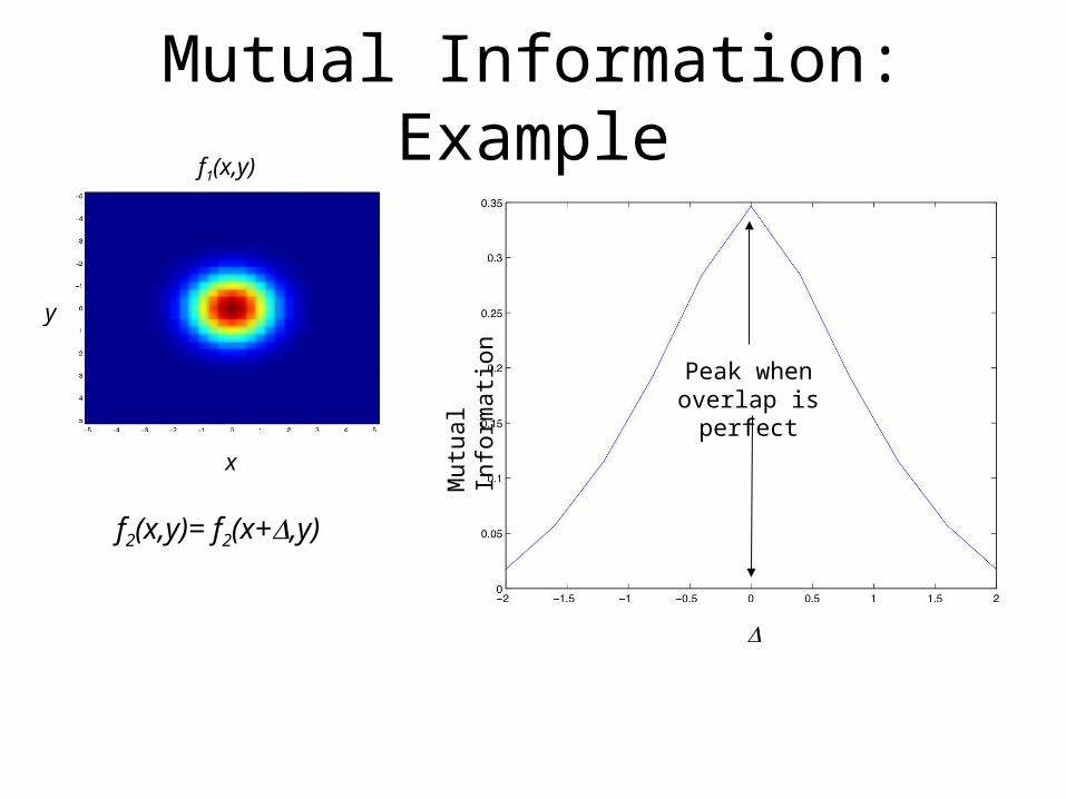
Mutual Information: Example
x
y
f1(x,y)
f2(x,y)= f2(x+,y)
Mut
ual I
nfor
mat
ion
Peak when overlap is perfect
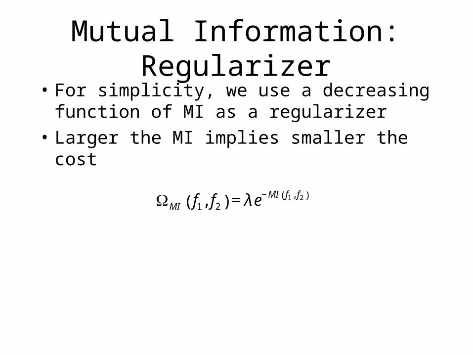
Mutual Information: Regularizer• For simplicity, we use a decreasing
function of MI as a regularizer
• Larger the MI implies smaller the cost
ΩMI f1, f2( ) = λ e−MI f1 , f2( )
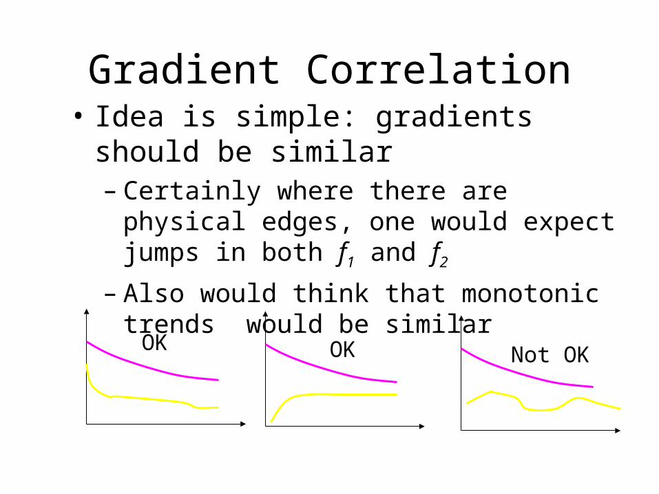
Gradient Correlation• Idea is simple: gradients should be
similar– Certainly where there are physical edges,
one would expect jumps in both f1 and f2
– Also would think that monotonic trends would be similar
OK Not OKOK

A Correlative Approach• A correlation coefficient based metric
∇f1T∇f2( )
2
∇f1 2
2∇f2 2
2 ≤ 1⇒
Ωcc f1, f2( ) = λ∇f1 2
2∇f2 2
2
∇f1T∇f2( )
2 −1⎡
⎣
⎢⎢
⎤
⎦
⎥⎥
2
∈ 0,∞( )
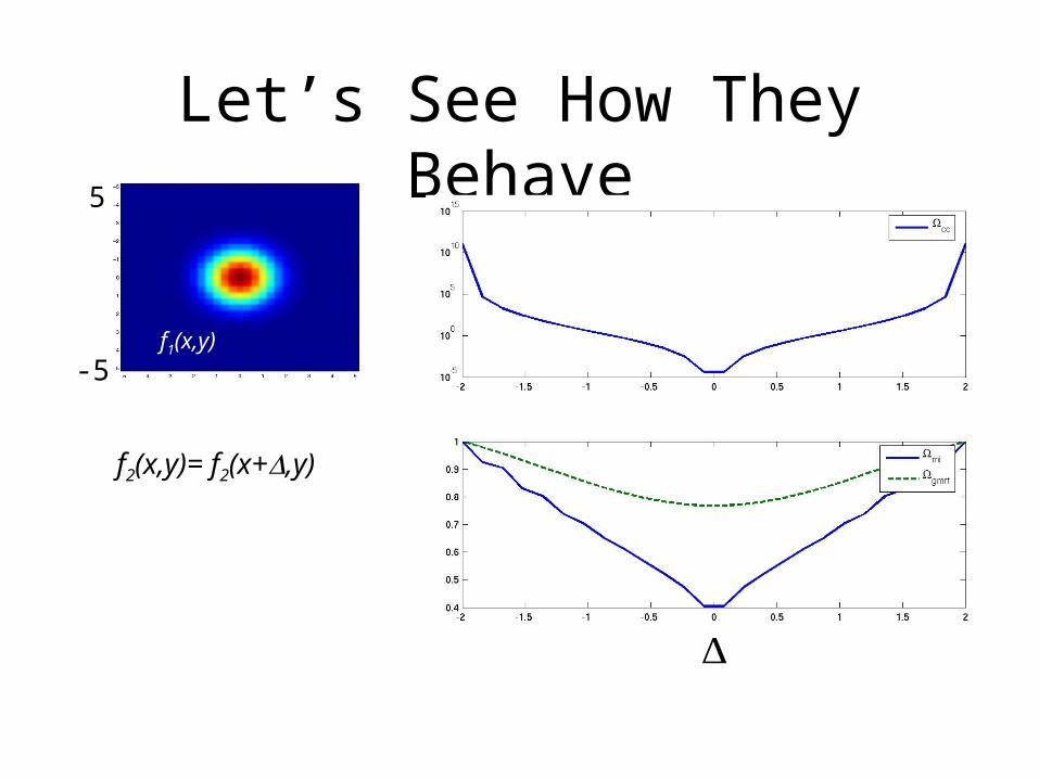
Let’s See How They Behave
f1(x,y)
f2(x,y)= f2(x+,y)
5
-5
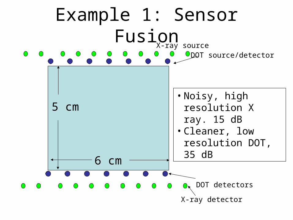
Example 1: Sensor Fusion
5 cm
6 cm
X-ray sourceDOT source/detector
DOT detectors
X-ray detector
• Noisy, high resolution X ray. 15 dB
• Cleaner, low resolution DOT, 35 dB
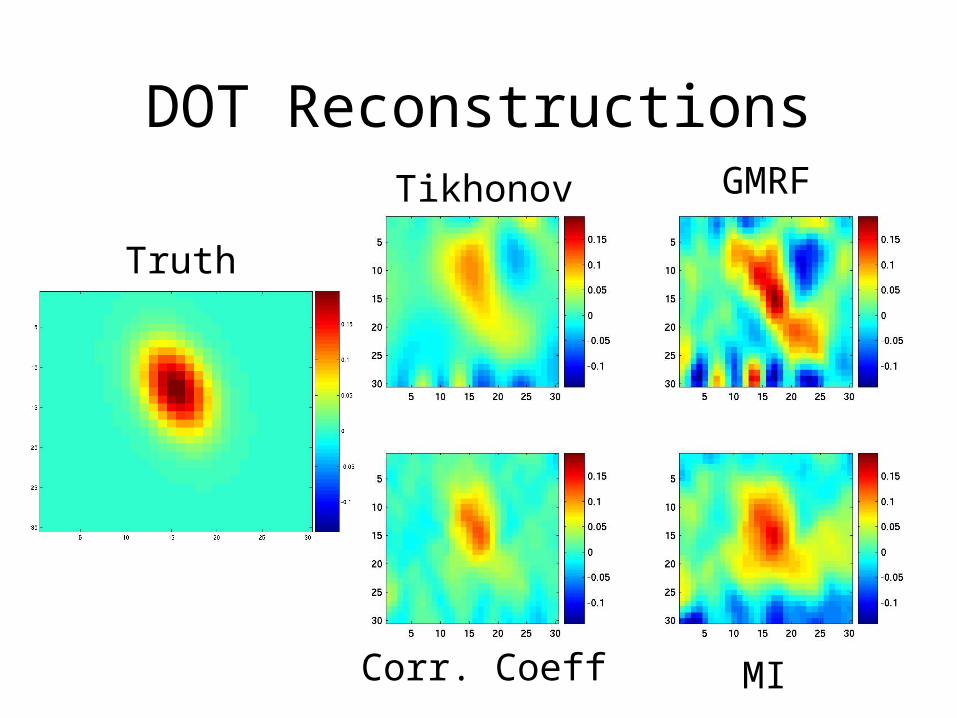
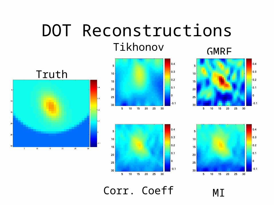
DOT Reconstructions
Truth
Tikhonov GMRF
Corr. Coeff MI
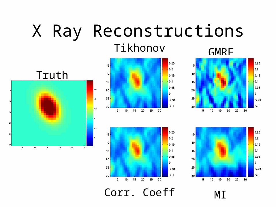
X Ray Reconstructions
Truth
Tikhonov GMRF
Corr. Coeff MI
DOT Reconstructions
Truth
Tikhonov GMRF
Corr. Coeff MI

X-ray Reconstructions
Truth
Tikhonov GMRF
Corr. Coeff MI

Mean Normalized Square ErrorTikhonov GMRF Corr. Coeff MI
Whole region 0.84 1.27 0.30 1.05Anomaly only 0.25 0.18 0.11 0.12
Tikhonov GMRF Corr. Coeff MIWhole region 0.28 0.54 0.27 0.46Anomaly only 0.08 0.12 0.08 0.10
Tikhonov GMRF Corr. Coeff MIWhole region 0.17 0.42 0.09 0.09Anomaly only 0.06 0.14 0.03 0.03
Tikhonov GMRF Corr. Coeff MIWhole region 0.13 0.33 0.12 0.13Anomaly only 0.04 0.07 0.04 0.04
DOT
X Ray
DOT
First Example
Second Example
X Ray
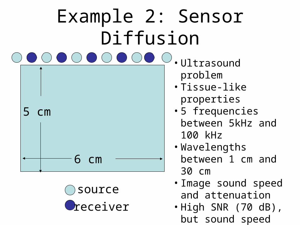
Example 2: Sensor Diffusion
5 cm
6 cm
source
receiver
• Ultrasound problem• Tissue-like properties • 5 frequencies between
5kHz and 100 kHz• Wavelengths between
1 cm and 30 cm• Image sound speed
and attenuation• High SNR (70 dB), but
sound speed about 20x absorption and both in cluttered backgrounds
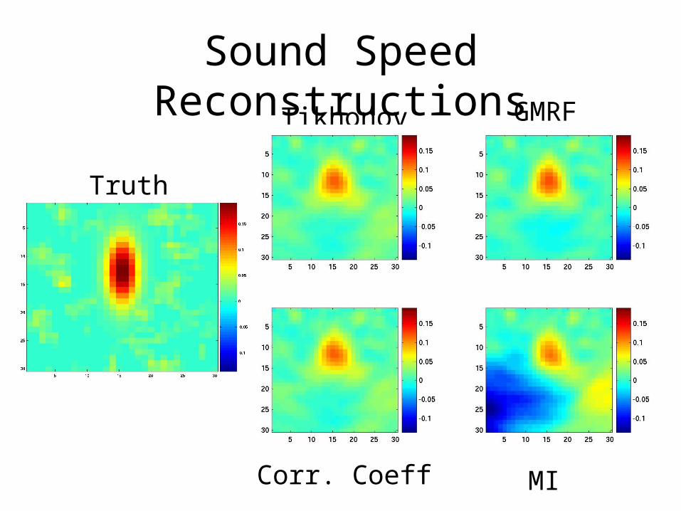
Sound Speed Reconstructions
Truth
Tikhonov GMRF
Corr. Coeff MI
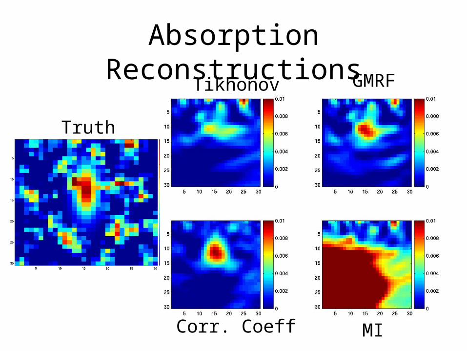
Absorption Reconstructions
Truth
Tikhonov GMRF
Corr. Coeff MI
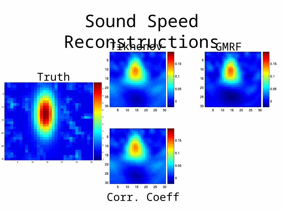
Sound Speed Reconstructions
Truth
Tikhonov GMRF
Corr. Coeff
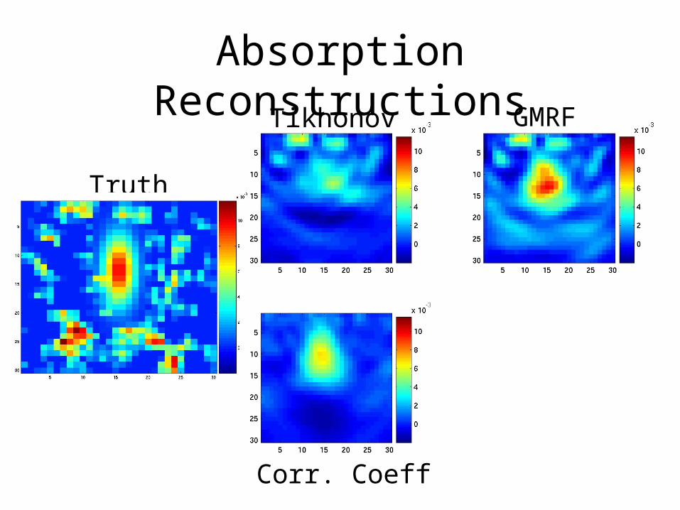
Absorption Reconstructions
Truth
Tikhonov GMRF
Corr. Coeff
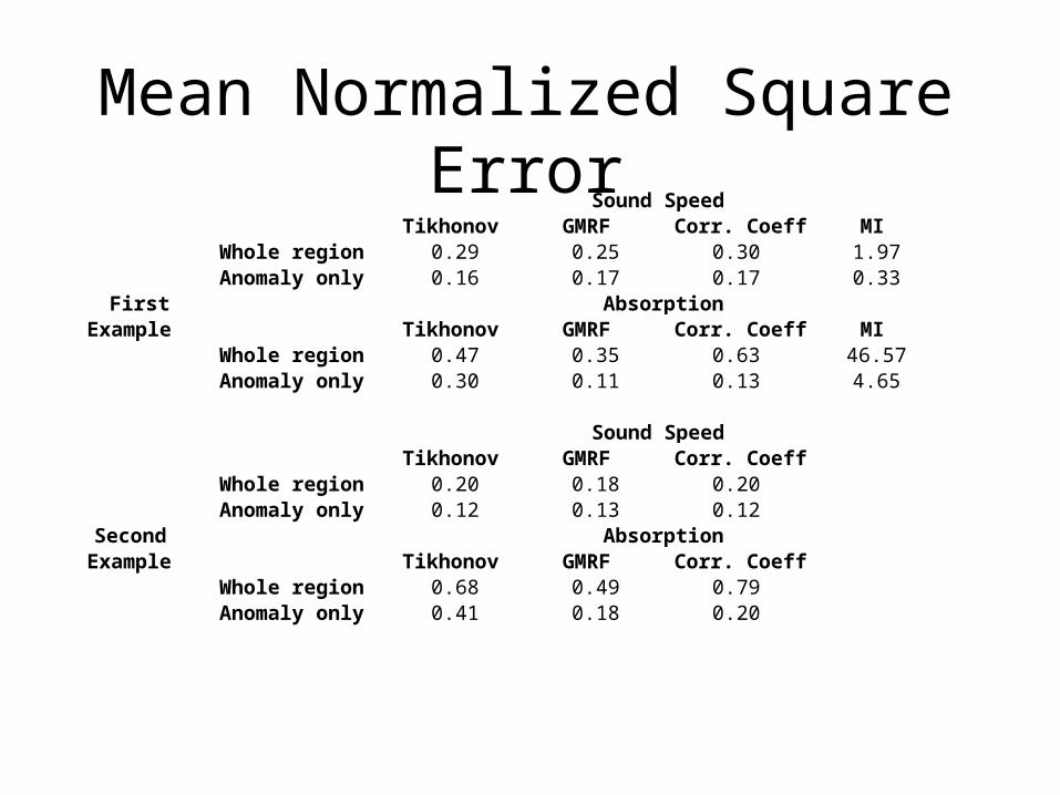
Mean Normalized Square ErrorTikhonov GMRF Corr. Coeff MI
Whole region 0.29 0.25 0.30 1.97Anomaly only 0.16 0.17 0.17 0.33
Tikhonov GMRF Corr. Coeff MIWhole region 0.47 0.35 0.63 46.57Anomaly only 0.30 0.11 0.13 4.65
Tikhonov GMRF Corr. CoeffWhole region 0.20 0.18 0.20Anomaly only 0.12 0.13 0.12
Tikhonov GMRF Corr. CoeffWhole region 0.68 0.49 0.79Anomaly only 0.41 0.18 0.20
Absorption
First Example
Second Example
Sound Speed
Absorption
Sound Speed
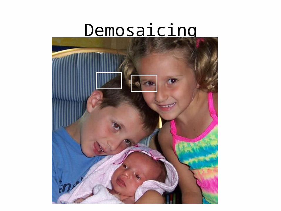
Demosaicing
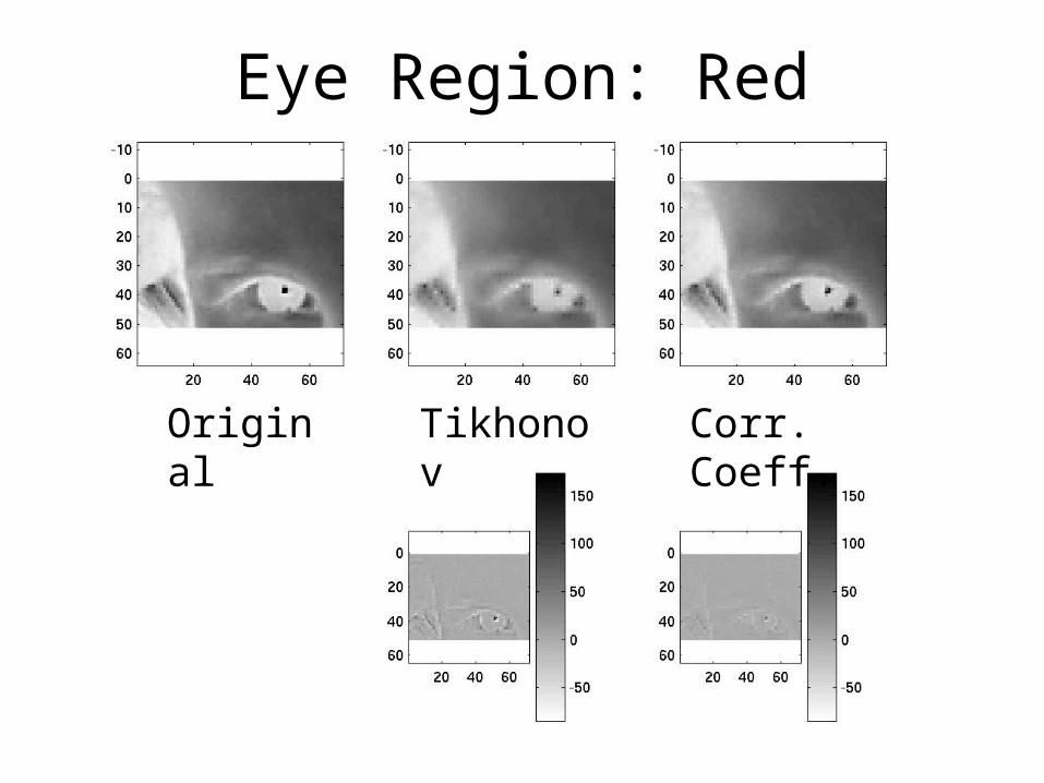
Eye Region: Red
Original Tikhonov Corr. Coeff.
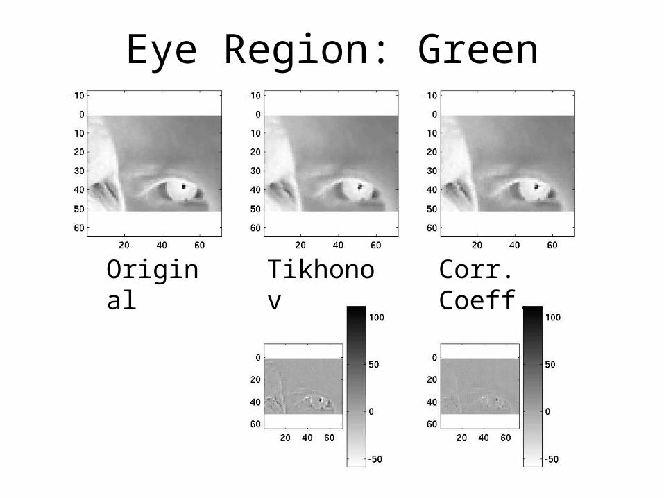
Eye Region: Green
Original Tikhonov Corr. Coeff.
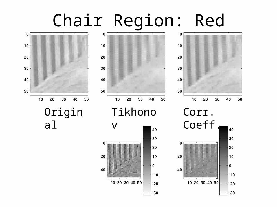
Chair Region: Red
Original Tikhonov Corr. Coeff.
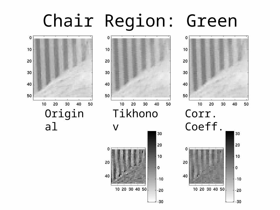
Chair Region: Green
Original Tikhonov Corr. Coeff.
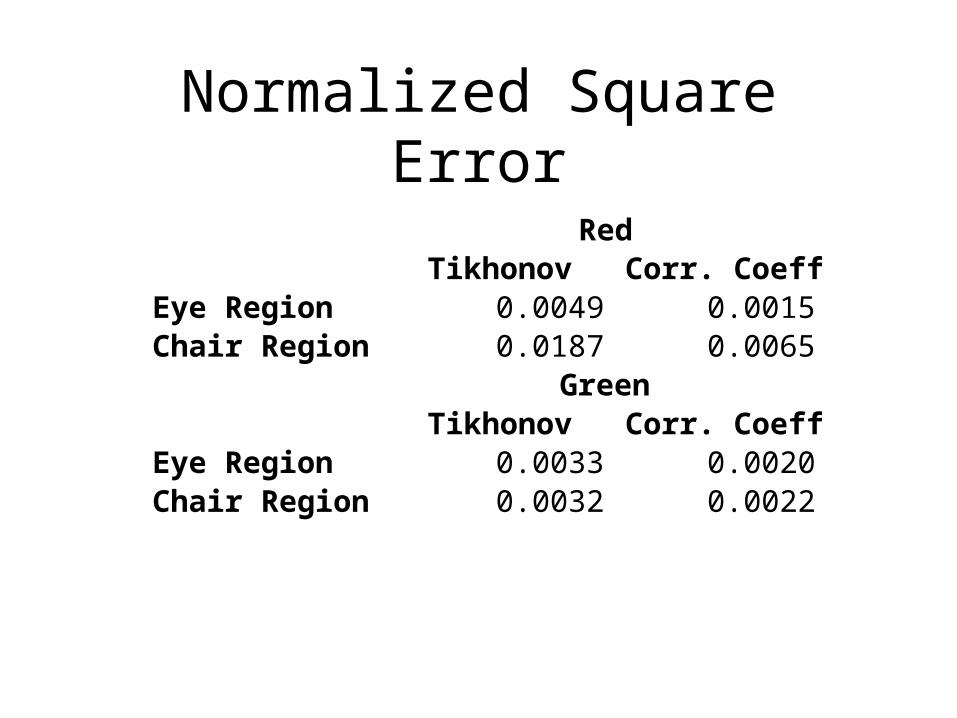
Normalized Square Error
Tikhonov Corr. CoeffEye Region 0.0049 0.0015Chair Region 0.0187 0.0065
Tikhonov Corr. CoeffEye Region 0.0033 0.0020Chair Region 0.0032 0.0022
Red
Green
Conclusions etc.• Examined a number of methods for building
similarity into inverse problem involving multiple unknowns
• Lots of things that could be done– Objective performance analysis. Uniform CRB
perhaps– Parameter selection, parameter selection,
parameter selection– 3+ unknowns– Other measures of similarity